Battle and Beating, Water and Waste

Micro-Level Impact Evaluation in Developing and

Emerging Economies

Dissertation

zur Erlangung des wirtschaftswissenschaftlichen Doktorgrades

der Wirtschaftswissenschaftlichen Fakultät der Georg-August-Universität Göttingen

vorgelegt von

Dipl. Oec. Johannes Peter Rieckmann, M.A.

aus Göttingen

Göttingen, 2014

2

Erstgutachter: Prof. Stephan Klasen, Ph.D.

Zweitgutachter: Prof. Dr. Axel Dreher

Drittprüfer: Jun.-Prof. Dr. Sebastian Vollmer

Tag der mündlichen Prüfung: 07. Februar 2014

Kapitel II dieser Dissertation gleichzeitig erschienen in Journal of Development Effectiveness Bd. 4

Heft 4, Seiten 537 – 565, London, 2012.

3

Acknowledgements

Almost five years of work found their way into this dissertation thesis. This fulfilling time was rich of

variation, professional challenges and new experiences. I am grateful to Prof. Stephan Klasen, Ph.D.

for providing me with the opportunity to work on a very interesting impact evaluation project in

Yemen; and as a research associate at the Chair of Economic Theory and Development Economics. I

would like to thank him for his supervision, advice and guidance through the process of writing my

thesis. I am further indebted to Prof. Dr. Axel Dreher for his willingness to act as second advisor, and

to Assistant Prof. Dr. Sebastian Vollmer who agreed to resume the role of the third examiner.

All of this would not have been possible without the life-long support by my parents and brothers, on

whom I can depend unconditionally. I am grateful to my grandmother for her encouragement. I am

indebted to Karoline, whose patience and understanding helped me along the rocky road of finalising

this thesis.

Particular thanks go to my close friends and fellow students from my Alma Mater at Bremen, André

Statler and Stefan Waldorf, for their invaluable input in countless “technical” discussions; for

comradeship and moral support. The same is true regarding my close friend and grammar school

mate Fabinzel, whose highlighting of the important things in life helped me focusing more than once.

It was my privilege to work with alert and amiable colleagues. While I cannot list here all of them,

some of them became friends and deserve a special mention. I would like to express my deep

appreciation for Dominik’s collaboration as a co-author and canteen mate, with whom I shared office

and interests. I am grateful to Kristina for her cooperative teamwork. I thank my office mate Nils for

teamwork in teaching, and tips and tricks regarding research and writing. I am grateful to Malte for

subject-specific input; and to Carsten for frequently helping me looking over the rim of a coffee cup

onto the bright side of life. Further thanks go to the Schlözis, Dimi, Jan, Lore, Merle, Mo, Nicolas,

Simon, Sophia, Steffen, and all those other folks who added to an enriching time in Göttingen.

Göttingen, December 2013

4

5

Table of contents

Acknowledgements ................................................................................................................................. 3

List of abbreviations .............................................................................................................................. 10

Introduction ........................................................................................................................................... 13

Synopsis of Chapter I ............................................................................................................................. 15

Synopsis of Chapter II ............................................................................................................................ 16

Synopsis of Chapter III ........................................................................................................................... 17

Chapter I: Violent behaviour – the effect of civil conflict on domestic violence in Colombia ........... 19

I.1 Introduction ....................................................................................................................... 20

I.2 Theory and literature review ............................................................................................. 22

I.3 Data and empirical strategy .............................................................................................. 26

I.4 Analysis and results ........................................................................................................... 32

I.4.1 General models ............................................................................................................. 32

I.4.2 Alternative spatial identification and simulation of effect’s magnitude ....................... 35

I.4.3 Alternative measures of domestic violence .................................................................. 36

I.4.4 Possible endogeneity issues .......................................................................................... 37

I.5 Conclusion ......................................................................................................................... 42

Chapter II: Benefits trickling away – the health impact of extending access to piped water and sanitation in urban Yemen ................................................................................................................... 43

II.1 Introduction ....................................................................................................................... 44

II.2 Background ........................................................................................................................ 46

II.2.1 Literature review ....................................................................................................... 46

II.2.2 Project description .................................................................................................... 49

II.3 Data and empirical strategy .............................................................................................. 51

II.3.1 Data ........................................................................................................................... 51

II.3.2 Empirical strategy ...................................................................................................... 53

II.4 Results ............................................................................................................................... 56

II.4.1 Project impact ........................................................................................................... 56

II.4.2 Sources of water pollution ........................................................................................ 63

II.5 Conclusion ......................................................................................................................... 65

6

Chapter III: Determinants of drinking water treatment and hygiene habits in provincial towns in Yemen ................................................................................................................................................... 67

III.1 Introduction ....................................................................................................................... 68

III.2 Literature review and hypotheses ..................................................................................... 72

III.3 Programme background and data ..................................................................................... 78

III.4 Methodology and empirical strategy ................................................................................ 84

III.5 Results ............................................................................................................................... 86

III.5.1 Drinking water treatment .......................................................................................... 86

III.5.2 Use of cleanser for hand washing ............................................................................. 91

III.6 Conclusion ......................................................................................................................... 96

Bibliography ......................................................................................................................................... 101

Appendix A: Supplementing Chapter I ............................................................................................. 115

A.1 Data ..................................................................................................................................... 115

A.2 Technical notes .................................................................................................................... 116

A.3 Estimation results ................................................................................................................ 118

A.4 Geography ........................................................................................................................... 120

Appendix B: Supplementing Chapter II ............................................................................................ 123

B.1 Description of covariates ..................................................................................................... 123

B.2 Descriptive statistics ............................................................................................................ 125

B.3 Estimation results ................................................................................................................ 127

B.4 Pollution pattern ................................................................................................................. 129

Appendix C: Supplementing Chapter III ........................................................................................... 131

C.1 Technical notes .................................................................................................................... 131

C.2 Description of covariates ..................................................................................................... 133

C.3 Descriptive statistics ............................................................................................................ 135

C.4 Methodology of employed instrumental variable approaches ........................................... 136

C.5 Robustness checks in context of mapping hygiene habits .................................................. 143

C.6 Estimation results ................................................................................................................ 154

C.7 Geography ........................................................................................................................... 175

Eidesstattliche Versicherung ............................................................................................................... 177

Personal details and educational background .................................................................................... 179

7

List of tables

Table I.1: Summary statistics: all women who live with their partner .................................................. 30

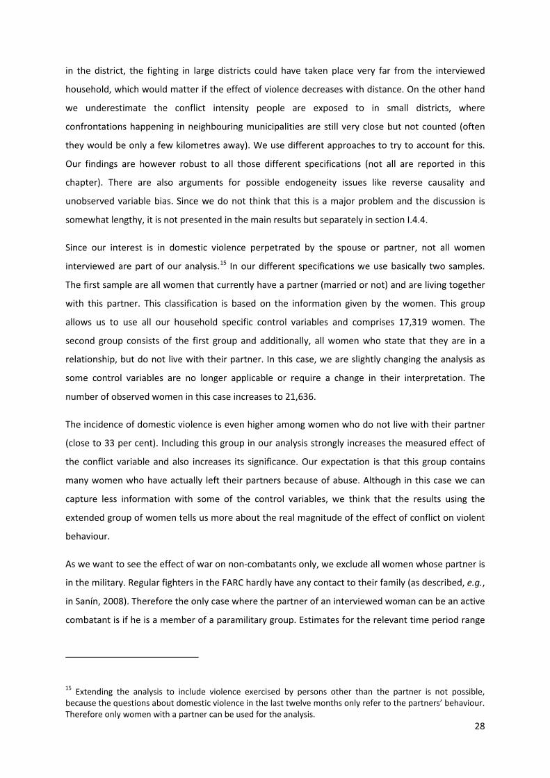
Table I.2: Summary statistics: districts separated by conflict intensity ................................................. 31

Table I.3: Probit regression; dep. variable: physical domestic violence last 12 months ....................... 33

Table I.4: Regression domestic violence, IV two-stage regression models ........................................... 40

Table II.1: Disease burden among household members ....................................................................... 57

Table II.2: Propensity score matching – impact of water ...................................................................... 58

Table II.3: Propensity score matching – impact of sanitation ................................................................ 59

Table II.4: Instrumental variable analysis – impact of water ................................................................. 60

Table II.5: Instrumental variable analysis – impact of sanitation .......................................................... 60

Table II.6: Double difference results for water and sanitation .............................................................. 61

Table III.1: Household sample, by region and connection status .......................................................... 81

Table III.2: Drinking water treatment, relative frequencies by location and connection status ........... 87

Table III.3: Probability of drinking water treatment, connections compared, selected specifications . 88

Table III.4: Use of cleanser for hand washing, relative frequencies by location and connection group 91

Table III.5: Probability of cleanser use, connections compared, selected specifications ...................... 93

Table A.1: Definitions of domestic violence ........................................................................................ 115

Table A.2: Probit regression; alternative dependent variables ........................................................... 118

Table A.3: Negative Binomial regression; dep. var. no. armed confrontations 2003/04 ..................... 119

Table B.1: Household sample .............................................................................................................. 125

Table B.2: Socio-economic characteristics in treatment and control groups ...................................... 125

Table B.3: Contamination of drinking cup ........................................................................................... 126

Table B.4: Change of pollution between storage tank and drinking cup ............................................. 126

Table B.5: IV Regressions – children age zero to five years ................................................................. 127

Table B.6: IV Regressions – all ages ..................................................................................................... 128

Table C.1: Description of covariates .................................................................................................... 133

Table C.2: Means and differences of outcomes by connection status ................................................ 135

Table C.3: Mean spending (per capita, in YER) on cleanser by location and connection status ......... 135

8

Table C.4: Mean spending (per capita, in YER) on soap by location and connection status ............... 143

Table C.5: Spending on soap, connections compared, selected specifications ................................... 146

Table C.6: Spending on cleanser, connections compared, selected specifications ............................. 148

Table C.7: Mean frequency of latrine-cleaning by location and connection status ............................ 149

Table C.8: Latrine-cleaning frequency, connections compared, selected specifications..................... 150

Table C.9: Probability of drinking water treatment, piped water, ICT covariates ................................ 154

Table C.10: Probability of drinking water treatment, sewerage, ICT covariates ................................. 155

Table C.11: Probability of drinking water treatment, piped water, other specifications & estimators 156

Table C.12: Probability of drinking water treatment, sewerage, other specifications & estimators .. 157

Table C.13: Probability of cleanser use, piped water, ICT covariates .................................................. 158

Table C.14: Probability of cleanser use, sewerage, ICT covariates ...................................................... 159

Table C.15: Probability of cleanser use, piped water, other specifications & estimators ................... 160

Table C.16: Probability of cleanser use, sewerage, other specifications & estimators ....................... 161

Table C.17: Spending on soap, piped water, ICT covariates ................................................................ 162

Table C.18: Spending on soap, sewerage, ICT covariates .................................................................... 163

Table C.19: Spending on soap, piped water, other specifications & estimators ................................. 164

Table C.20: Spending on soap, sewerage, other specifications & estimators ..................................... 165

Table C.21: Spending on cleanser, piped water, ICT covariates ........................................................... 166

Table C.22: Spending on cleanser, sewerage, ICT covariates ............................................................... 167

Table C.23: Spending on cleanser, piped water, other specifications & estimators ............................ 168

Table C.24: Spending on cleanser, sewerage, other specifications & estimators ................................ 169

Table C.25: Latrine-cleaning frequency, piped water, ICT covariates .................................................. 170

Table C.26: Latrine-cleaning frequency, sewerage, ICT covariates ...................................................... 171

Table C.27: Latrine-cleaning frequency, piped water, other specifications & estimators ................... 172

Table C.28: Latrine-cleaning frequency, sewerage, other specifications & estimators ....................... 173

Table C.29: IV estimator first stage results, connection to piped water and to improved sewerage .. 174

9

List of figures

Figure II.1: Water supply chain and test points ..................................................................................... 50

Figure II.2: Differences in diarrhoea incidence between treatment and control towns ....................... 62

Figure A.1: Surveyed districts in Colombia .......................................................................................... 120

Figure A.2: Conflict intensity ............................................................................................................... 121

Figure B.1: Spatial distribution of e.coli-polluted storage tanks (coastal) ........................................... 129

Figure C.1: Geographic location of survey towns ................................................................................ 175

10

List of abbreviations

Abbreviation Description 2SLS 2-stage Least Squares estimation procedure 2SPrB Two-stage Probit Bootstrap estimation procedure ATE Average Treatment Effect ATT Average Treatment effect for the Treated AUC Autodefensas Unidas de Colombia, United Self-Defence Forces of Colombia BMZ Bundesministerium für Wirtschaftliche Zusammenarbeit, German Federal Ministry of

Economic Cooperation and Development CGIAR-CSI Consultative Group on International Agricultural Research – Consortium for Spatial

Information CIAT Centro Internacional de Agricultura Tropical, International Centre for Tropical

Agriculture confrt. Confrontations CRC-PEG Courant Research Centre “Poverty, Equity and Growth in Developing Countries” CSO Yemenite Central Statistical Organization DALY Disability-Adjusted Life Years DANE Departamento Administrativo Nacional de Estadística, Colombian national statistics

department DAS Departamento Administrativo de Seguridad, Colombian Administrative Security

Department DD Double Differencing DFG Deutsche Forschungsgemeinschaft, German Research Foundation DHS Demographic and Health Survey DIVIPOLA DIVIsión POLítico Administrative, political administrative division DIW Deutsches Institut für Wirtschaftsforschung, German Institute for Economic Research Dr. Doktor, doctor Durat° Duration e.coli Escherichia coli, a bacterium Edu. Education e.g. Exempli gratia, for the sake of example EBV Endogenous Binary Variable ESRI Company and supplier GIS software, and geospatial vector data format et al. Et alii, and others etc. Et cetera, and so forth et seqq. Et sequentia, and those following FAO Food and Agriculture Organization of the United Nations FARC Fuerzas Armadas Revolucionarias de Colombia, Revolutionary Armed Forces of

Colombia FRA Forest Resources Assessment GIS Geographic Information System GPS Global Positioning System HH Household i.e. Id est, that is ibid. Ibidem, the same place

11

ICT Information and Communication Technology IGAC Instituto Geográfico Agustín Codazzi, Geographic institute Agustin Codazzi IV Instrumental Variable IVP Instrumental Variable Probit estimation procedure JEL Journal of Economic Literature KfW Kreditanstalt für Wiederaufbau, German Development Bank LATE Local Average Treatment Effect, see ATT LDV Limited Dependent Variable MENA Middle East and North African region MNSSD Middle East and North Africa Sustainable Development Sector Department N Sample Size No./ # Number ODC Observatorio de Drogas de Colombia, Colombian Drug Observatory OLS Ordinary Least Squares p. Page Part. Partner’s Ph.D. Philosophiae doctor, Doctor of Philosophy pp. Pages Prof. Professor, professor PSM Propensity Score Matching PTOP Provincial Towns Program PTSD Posttraumatic Stress Disorder R² Coefficient of determination RCT Randomized Controlled Trial Resp. Respondent’s RSUR BP Recursive Seemingly Unrelated Biprobit estimation procedure SD Standard Deviation SIG-OT Sistema de Información Geográfica para la planeación y el Ordenamiento Territorial,

Geographic Information System for Planning and Territorial Regulation SRTM Shuttle Radar Topography Mission SUR BP Seemingly Unrelated Biprobit estimation procedure USD United States Dollars W2SLS Wooldridge 2-stage Least Squares estimation procedure YER Yemenite Rial, currency Yrs Years

12

13

Introduction

“If the numbers we see in domestic violence were applied to terrorism or gang violence, the entire

country would be up in arms, and it would be the lead story on the news every night.”

Congressman Mark Andrew Green1

“The General Assembly […] 1. Recognizes the right to safe and clean drinking water and sanitation as

a human right that is essential for the full enjoyment of life and all human rights; […].”

General Assembly of the United Nations2

Empirical analysis in the domain of development economics has been coined by the macroeconomic

perspective for decades. It is a comparatively recent evolvement that a string of literature focusing

on micro-level data branches off – or, much more to the point, supplements and widens – this well-

established field of analytical and explorative studies. Furthermore, both policy-makers and scholars

display an intensified interest in uncovering and quantifying the effects which particular

environmental conditions and human behaviour on the household and individual level have on

individual wellbeing. The work at hand aims at contributing to the knowledge base which this

extension of the academic discipline is generating. To this end, the findings of econometric impact

evaluations – which constitute the common thread running through this dissertation – conducted in

two different areas of day-to-day life in developing and emerging economies are presented.

The first of these areas is the behavioural response of people living in spatial vicinity of violent

conflict. Violence makes life miserable. Since now more than two decades the world has been

becoming a less predictable and more insecure environment for large shares of the world population.

Relatively stable geopolitical powers opposing each other and controlling large spheres of interest

have been successively replaced by more fluid, opaque and less spacious theatres of conflict. The

pending threat of interstate war between geographically separated parties pursuing power-political

interests and – at least allegedly – ideological goals has been replaced by actual and multiple

eruption of civil and so-called low-intensity conflict; and asymmetric warfare. It appears that

bloodshed has not become less prevalent than before. Struggles today are often rooted in

1 Former member of the United States House of Representatives Mark Andrew Green, Wisconsin, quoted in Colorado Department of Human Services (2010). 2 Quoted from Resolution 64/292 (United Nations General Assembly, 2010), passed 28 July 2010, 108th plenary meeting.

14

unmanaged ethnic friction, diverging religious convictions, and competition for natural resources.

The dividing line between combatants and civil population has eroded and become more permeable

than before, which is closely linked with larger shares of the civil population being victimised by – or

witnessing extreme forms of – physical force. Exposure of its members to violence backfires on

society. It severely affects individual wellbeing and development potentialities, and often instils

further violent behaviour. Getting granular on the impact of such exposure on the prevalence of

domestic violence, the first chapter of this dissertation thesis provides scientific tesserae contributing

to estimating a societal price-tag of warlike row; and its repercussions on interpersonal relationships

and social behaviour towards family and friends. In the long run, inter-generational consequences of

domestic violence as for example stunting of personality development of children hamper

macroeconomic development.

The second area of interest is revolving around the most important resource on earth. Without

water, there is no life. With polluted drinking water, life is miserable. Quality of life is reduced by

illness; and for still far too many of the weakest members of society – the children – even its

duration. In developing countries diarrhoeal diseases account for the majority of child mortality, with

almost nine out of ten cases of death by diarrhoea caused by bad water and sanitation conditions

(Black, Morris and Bryce 2003). According to the United Nations Target 7.C of the Millennium

Development Goals (“Halve, by 2015, the proportion of the population without sustainable access to

safe drinking water and basic sanitation”, see United Nations, 2013) was met five years early,

regarding drinking water. Still, lack of access remains an issue in urban agglomerations of Central Asia

and the Caucasus, as well as in numerous rural regions all over the developing world. The current

situation is less auspicious regarding sanitation. More than half of the world population does not yet

benefit from regular access. The second chapter studies the impacts of connection of households to

piped water and improved sewerage on health, school and workplace attendance.

It can be frequently observed that piped water, after having been purified at treatment plants and

supplied germfree, gets re-contaminated within households. Conducting water quality testing at

different points of the intra-household supply chain allows answering where and often also how the

pollution takes place. The lion’s share of this deterioration of water quality is linked to behavioural

aspects of water handling and hygiene rather than to constructional features. The obvious follow-up

question reads: why does the recontamination takes place, i.e. which conditions are the drivers

behind those behavioural aspects? The third chapter builds upon the second; and addresses this

question. Here the determinants of intra-household behaviour regarding water handling and hygiene

are scrutinized, and linked with Chapter II.

15

Synopsis of Chapter I, on the effect of civil conflict on domestic violence in Colombia

Experience and direct witnessing of severe violence leave its marks on a person’s mind set and

personality. The same is true – albeit to a lesser extent – for frequent and prolonged indirect

exposure by, e.g., news reports about violent incidents in spatial proximity of the person’s social

circle. The psychological cost of living in a war zone has to be borne by the persons themselves as

well as their next of kin. Attitudes tend to shift towards higher levels of acceptance of violence as a

means of social interaction and settling dispute.

The term attitude is a somewhat elusive concept; and its individual characteristics are hard to

observe. What can be observed, though, are behavioural aspects attitude manifests itself in. Often,

interpersonal behaviour of people who mentally suffer from what they felt saw and heard of shifts

towards more violent patterns itself. The constant tension created by an insecure environment and

deprivation of areas of retreat in conjunction with emotional blunting increases, for example, the

probability of incidence of domestic violence. The change of incidence of domestic violence is

therefore exploited in this chapter as an indicator of change of attitude.

This chapter is joint work, written together with Dominik Noe. It contributes to the string of literature

assessing the medium and long term consequences of civil conflict on society. We postulate the

theory that living in households in proximity to locations where incidents of extreme violence occur

increases the probability of women living in these households to become victims of domestic

violence. This theory is then tested using data from Colombia as a country where both rich data on

incidence of violent clashes as well as of domestic violence is available.

The core finding is that higher intensity of conflict increases the probability of women to be subject

to domestic violence.

16

Synopsis of Chapter II, on the health impact of extending access to piped water and

sanitation in urban Yemen

Supply of safe drinking water and hygienic wastewater disposal are considered to be basic

prerequisites for human health and development, especially in urban agglomerations. While

sustainable provision with this fundamental infrastructure alone poses challenges in towns around

the developing world, water scarcity often exacerbates the endeavour further. The combination of

high population growth and groundwater overuse is a phenomenon that can be observed in various

countries of the Middle East and North Africa.

Over the recent decades, both governments of recipient countries as well as international donors

have developed a pronounced interest in evaluating and measuring the impact of construction of

piped water and improved sewerage networks on health, education, income, labour time and

aspects of livelihood. The goal is to increase effectiveness and efficiency of resource allocation, to

improve sustainability, and to learn about disruptive factors which often appear to dilute the

intended benefits.

This chapter is joint work, written together with Stephan Klasen, Tobias Lechtenfeld, and Kristina

Meier. It contributes to the presently still manageable array of impact evaluations in the water and

sanitation sector, and to the authors’ knowledge is the first rigorous one in the urban environment.

The connection of households in provincial towns to piped water and improved sewerage in two

different topographic regions of Yemen is investigated with respect to its impacts on health, as well

as resultant school and workplace attendance of the household members. Quasi-experimental

methods and water quality tests in presence of variation of infrastructure proliferation allow

identifying these impacts separately for mere connection to piped water, and for additional

connection to improved sewerage.

The core finding is that connection to piped water in the Yemenite towns can do harm when water

supply is intermittent, and does not change much in presence of reliable one compared to traditional

and alternative solutions of water supply. Anyhow, connection to improved sewerage comes with

health benefits when water supply is reliable.

17

Synopsis of Chapter III, on determinants of drinking water treatment and hygiene habits in

urban Yemen

One of the goals that infrastructure construction projects in the water and sanitation sector aim to

achieve is improvement of health of beneficiary population. The frequently observed dilution of

intended health benefits of this utility infrastructure is only partly rooted in technical aspects of the

supply side, such as intrusion of wastewater into drinking water feed pipes. Just as little can the

remainder of the dilution be attributed entirely to environmental aspects, such as unanticipated

rapid population growth and depleting ground water tables. Evidence suggests that behavioural

aspects on the demand side – i.e., within the connected households – have to be blamed for

considerable complicity.

This is also the case for a respectable share of the Yemenite households the reader already will have

become acquainted with in Chapter II. Drinking water quality is observed to deteriorate in those

households from the point of feeding – usually a supply pipe leading from street level to a roof or

courtyard storage tank – to the point of use. Technical considerations as well as particularities of

microbiological contamination strongly hint towards pollution occurring due to water handling and

hygiene practises in need of improvement.

Chapter III builds upon the findings of the preceding Chapter II, doing some “detective” work in

search of what is behind the lack of desirable health impacts. It contributes to the literature

identifying drivers of human behaviour regarding water handling and general hygiene. In order to

shed light on the conducive and impedimental factors having a hand in the matter, self-reported

behaviour is related to overarching characteristics of households; and individual characteristics of

household heads. Those factors which can be influenced in the short to medium term are of special

interest, as they are most relevant for policy implication.

The core finding is that hygiene training, access to information and communication technology, and

school education are among the relevant controllable determinants of water handling and hygiene

behaviour. Policy implications are to invest in these three domains. Connection to piped water and

improved sewerage – which typically can be widened out only in the medium to long term – is

fostering desirable behaviour as well, albeit to a lesser extent, and with the effect of the former

exceeding that of the latter.

I provide three suggestions answering the arising question how – regarding the seemingly

contractionary effect of connection to piped water and improved sewerage – the findings of Chapter

II and III can be reconciled. First, we might witness either an overcompensation of the beneficial

impact of water treatment and hygiene habits on health by the detrimental impact of infrastructure

18

connection. Second, water treatment (and less likely from my point of view, hygiene practices) at the

household level might – although implemented – be ineffective for some reason, possibly faulty

practices. Third, we might witness an adjustment reaction of learning households that increase their

efforts regarding water safety and hygiene in answer to the variation of piped water quality they

observe.

19

Chapter I: Violent behaviour – the effect of civil conflict on domestic violence in

Colombia

Joint work with Dominik Noe3

Abstract

In this chapter we analyse the impact of civil conflict on domestic violence in Colombia and find that

higher conflict intensity increases the likelihood of women to become a victim of domestic violence.

The idea behind our approach is that the experience of conflict changes behaviour, attitude and

culture. We consider domestic violence to be an observable outcome of this change in behaviour.

Taking advantage of the uneven spatial distribution of the conflict we assess its impact, using micro

data from Colombia.

Keywords: Domestic Violence, Conflict, Colombia, Crime, Spatial Identification

JEL classification: H56, J12

Acknowledgements

Together with my co-author I would like to thank Chris Müris for his help and methodological

support; as well as Walter Zucchini. Furthermore we would like to thank Stephan Klasen, Axel Dreher,

Philip Verwimp, and the participants of seminars in Bonn, Göttingen and Heidelberg as well as the

2011 Arnoldshain Conference for helpful contributions. We are much obliged to James A. Robinson

for his helpful comments at the 2012 Nordic Conference in Gothenburg, and the participants of the

2013 workshop of the Households in Conflict Network in Berkeley. Financial support by the German

Research Foundation (DFG) through the Courant Research Centre “Poverty, Equity and Growth in

Developing Countries” (CRC-PEG) is gratefully acknowledged.

3 Courant Research Centre "Poverty, Equity and Growth", Georg-August-University Göttingen, Wilhelm-Weber-Str. 2, 37073 Göttingen, Germany, email: dnoe@uni-goettingen.de

20

I.1 Introduction

It is often claimed that violence begets violence. This can mean that the one being stricken strikes

back. It can however also mean that witnesses of violent acts are influenced in their own behaviour

and therefore might exercise violence themselves.

The idea of this chapter is that the experience of fighting and bloodshed caused by a civil conflict will

change the behaviour and attitude of the population witnessing it, so that they will be more willing

to also use violence. If this was the case, conflict could create a self-reinforcing culture of violence

which would hinder its termination, slow down the recovery afterwards or increase the likelihood of

new fighting. Culture and attitude are hard to observe and therefore we use differences in

observable behaviour to check this hypothesis. Many forms of observable violence could be a direct

consequence of the conflict and not necessarily an expression of a behavioural change in the general

public. Domestic violence is an observable form of violent behaviour that is not likely to be a direct

consequence of a military conflict, but there are plausible mechanisms how the behavioural change

caused by such a conflict could lead to the use of violence within the family. The main channels

through which we expect conflict to increase domestic violence are increased acceptance of violence

if exposure of people to different forms of violence is augmented; and the function of domestic

violence as a stress release in an insecure environment.

This research aims at improving the understanding of the consequences of conflict. Blattman and

Miguel (2010) state that there is a lack of theory and evidence “in assessing the impact of civil war on

the fundamental drivers of long-run economic performance – institutions, technology and culture –

even though these may govern whether a society recovers, stagnates or plunges back into war”.4

While domestic violence is a crime and its investigation and prevention in itself an important issue,

we also use it as an indication of behavioural change. It is a threat for the security and cohesion of

society as it increases the violent potential for the future. This does not only refer to those people

whose behaviour has been changed by the conflict but also to later generations who suffer from this

domestic violence and are thereby negatively affected from childhood on.

In order to analyse the impact of civil conflict on behaviour, attitude and culture we use micro-data

from Colombia, considering domestic violence to be an observable outcome of changes in behaviour.

We find that a higher incidence of combat within a district significantly increases the likelihood of

women in this district to become a victim of domestic violence.

4 A prominent example for literature on the impact of violence on cultural norms is a paper written by Miguel, Saiegh and Satyanath (2011). The authors find a strong link between a professional football player’s violent conduct – measured by red and yellow cards attributed – with the civil conflict history in his country of origin.

21

Colombia was chosen for various reasons. Domestic violence is a very common phenomenon in the

country. In our sample up to 20 per cent of the interviewed women who are currently in a

partnership report physical abuse by their partners.5 This is very high compared to other countries.6

In our data only women were interviewed and therefore we cannot consider domestic violence from

women against men.

Today’s conflict in Colombia has its roots in the 1950’s and still continues. It involves different

guerrilla organizations, of which the most important today, are the Fuerzas Armadas Revolucionarias

de Colombia (FARC) and Ejército de Liberación Nacional (ELN). Originating as peasant organizations

especially the FARC became a highly organized and effective guerrilla army with thousands of

soldiers. As a defence against the guerrilla, private actors – mainly land owners – founded

paramilitary organizations which later on joined to become the Autodefensas Unidas de Colombia

(AUC). All non-state actors rely heavily on illegal means of financing. The most important sources are

drug production and trafficking, kidnapping and extortion. Although the illegal economy was not the

source of the conflict, it is probably a main cause for its duration and its intensification especially in

the 1990s.7

Despite the long duration of the conflict the state is still functioning, although not in complete

control over all of its territory. Because of the existence of such a functional state, high quality data

about the conflict is available. Very few countries display both the incidence and severity of conflict

on the one hand as well as the “rich micro-level data” (Steele, 2007) on the other hand, as is the case

in Colombia.

5 The recall period comprises the past twelve months. 12.4% of the women report to have been subject to violence by a person other than their partner before that period (see also Table A.1). Note that the lifetime prevalence cannot be found straightforwardly by summing up the two measures, as there will probably be an intersecting set. Also the non-captured prevalence of physical violence inflicted by the current partner longer than twelve months ago could be confounding, although in the other direction (thus underestimating lifetime prevalence). 6 The World Health Organization (García-Moreno et al., 2005) reports in its Table 4.1 exposure to at least one act of physical act of violence within the past twelve months ranging from 3.1% (urban Japan) to 29% (provincial Ethiopia); with a non-weighted mean of 14.8% (own calculation). Ten countries from Africa, Asia, Europe, Oceania and South America are part of the considered sample. Reported lifetime prevalence of domestic violence ranges between 13% (urban Japan) and 61% (provincial Peru). In Africa on average the situation seems to be particularly dire. Durevall and Lindskog (2013) report in their Table 2 prevalence rates of physical intimate partner violence in eight sub-Saharan countries. DHS data stem from 2005 to 2011, with a recall period of twelve months. Violence rates range between 10.7% (Burkina Faso) and 56% (Rwanda), with a non-weighted mean of 31% (own calculation). 7 For a short summary of the rather complicated conflict history and involved parties in Colombia since the mid-20th century, see, e.g., Steele (2007) and Garcés (2005). Sanín (2008) provides useful insight on the characteristics of the non-state “armies” entangled in these conflicts.

22

Our analysis is based on individual-level data from the year 2005. In order to identify the effects of

conflict we use the uneven spatial distribution of conflict intensity within the Colombian territory.

We find that a woman in a district with high conflict intensity has an up to ten percentage points

higher chance of being a victim of domestic violence than a woman in a district with average or lower

conflict intensity.

I.2 Theory and literature review

This chapter is based upon the idea that experiencing or witnessing violent manifestations of conflict

will increase the incidence of domestic violence in spatial proximity of these manifestations. This

means we expect a behavioural change of people due to conflict. The observation of behavioural

change is, in most cases, very difficult; and therefore there is not much empirical research in this

field. Two of the few exceptions are Voors et al. (2012) who find that people who experience

violence from conflict become more risk-seeking and have a higher discount rate; and Blattman

(2009) who finds victims of violence to show higher political activity.

We assume that the repeated and sustained witnessing of violent acts in the context of armed

combat affects the mind-set. It can lead to “widespread tacit tolerance and acceptance of the use of

physical violence to solve private and social problems” and ultimately to an omnipresent culture of

violence (see Fishman and Miguel, 2008, on decisions as a matter of culture; and Waldmann, 2007,

specifically on the case of Colombia). Acclimatization and role models influence the way conflicts are

resolved. This applies also within the framework of small social groups like the family, and all the way

down to intimate relationships (see, e.g., Adelman, 2003, on the effect of militarization). An

environment of violent crime in the community is “associated with elevated risks of both physical

and sexual violence in the family” (Koenig et al. 2006). Also, “community-level norms concerning wife

beating“ (ibid.) have a significant effect on occurrence rates, as well as on the consequences the

affected wives draw from the experience in terms of, e.g., divorce rates (Pollak, 2004). Wood (2008)

argues that “social processes may be reshaped by conflict processes”. Another factor might be the

“emotional blunting” of victims, witnesses or perpetrators as a consequence of their experiences.

This can lower the psychological threshold restraining the use of force at home. Post-traumatic stress

disorders can result from exposure to violence, and lead to changes of behaviour. It was found in the

United States that veterans with posttraumatic stress disorder (PTSD) are more often perpetrators of

domestic violence than the general population (Sherman et al. 2006). We expect a similar effect to

apply for witnesses of violence who were not directly involved in combat. We believe number and

intensity of violent outbreaks to increase due to this effect.

23

Domestic violence is usually divided into two categories, one of which is referred to as expressive,

the other one as instrumental. In the expressive form perpetrators gain utility from inflicting physical

harm on their partners or children by being able to express their feelings in a drastic way, and release

their emotional pressure (Winkel, 2007). Living in a conflict zone brings about a general and

unassigned feeling of threat, loss of control, helplessness and an elevated level of emotional stress

because the usual societal rules that bring a certain protection from physical and other harm do not

necessarily apply anymore when the actions of present armed combatants are incalculable. Passing

this pressure on onto others within the closest social environment in a “cyclist manner” – ducking

and kicking – may serve as a psychological relief valve for these people. When persons feel the

aforementioned loss of control they might use violence to prove having predominance at least over

their direct social environment, i.e., at least over some part of their life.

Long et al. (1991) describe not only this expressive aspect of utility creation for the perpetrator, but

also include an instrumental function of spouse-beating. Domestic violence in its instrumental

function is shaped and intended to modify the victim’s behaviour. It aims to “educate” the victim in

line with the interests of the perpetrator. The aforementioned emotional blunting will decrease

empathy for others and thereby the threshold to resort to violent coercion instead of verbal dispute.

A very important point about domestic violence is its acceptance or non-acceptance by the victims.

This is largely determined by cultural norms8 and the victim’s alternatives or exit options. If a victim is

economically dependent on the perpetrator it is very difficult to leave an abusive relationship; while,

e.g., a good education and an independent economic situation could facilitate the exit. Hidrobo and

Fernald (2013)9 point out that the effect of economic independence may be ambiguous, and “where

outside-of-marriage options are not a credible threat point and a power imbalance exists among the

couple” – the latter being triggered by unequal education levels of the partners – “violence is likely to

occur”. The authors report this to be “consistent with psychological theories of power, control, and

status inconsistency”. Also, additional income earned by the women could provoke contestation over

the money. Cultural and personal norms determine whether the victim will even recognize domestic

violence as an injustice and try to end the relationship; or just accept it as something normal.

Whether it is accepted or legally possible to end an abusive marriage also depends on the societal

background.

8 For instance, Kedir and Admasachew (2010) emphasize that victimised Ethiopian women tend not to resort to “institutional support” due to “general societal disapproval of such measures“. 9 Hidrobo and Fernald (2013) study the effect of an Ecuadorean cash transfer program.

24

Both sexes are represented among perpetrators and victims of domestic violence (see, for example,

Strauss, 1993, and Karnofsky, 2005). The majority of perpetrators are male domestic partners, while

most victims are female (e.g., Aizer, 2010). This also is the setting that we have to focus on in our

analysis due to data limitations. In an unsafe external environment both woman and men feel an

increased need for protection. We believe that one important source of protection is the closest

social environment, which is the family. If physical violence is commonplace in the geographical

vicinity of their homes, we suppose that people show an increased reluctance to leave this

protection. Compared to a situation without violent conflict, we therefore assume women to accept

and endure more domestic violence than they would in a peaceful external environment. Probably

this is even more the case for mothers who have to look after children. The fear of losing access to

their children could hinder the former to turn their back on the children’s father. Fear for the

children’s physical well-being also makes it difficult for mothers to leave them with their partner if he

is a potential threat to the children. In the presence of violent exterior threats it becomes more

crucial for the family to persist in order to serve as a protective environment. This function gains in

importance as in the “climate of uncertainty, distrust, and polarization” which comes along with

violent conflict, “traditional social networks of mutual aid might likewise weaken” (Wood, 2008). The

traditional role of the man as provider is widely accepted in Colombia. It can come along with a

higher threshold of accepted domestic violence compared to other societies, as women may feel

dependent (Karnofsky, 2005; see also Farmer and Tiefenthaler, 1997, on a resource-centred non-

cooperative model of domestic violence).

The spatial proximity of violent incidents to households is of relevance because closer events are

perceived to be much more threatening than distant ones. Events one learns about by word of

mouth or by direct witnessing are more terrifying than those which are taken notice of only from the

newspapers or television broadcasting. Studies have shown that an incident of extreme violence can

have distinct adverse psychological effects on people even if it happened thousands of kilometres

away from them. For example, the terror attack against the World Trade Center in Manhattan on

September 11th in 2001 has had a traumatizing effect on people all over the United States of America

(Silver et al. 2002). It seems more than comprehensible that combat taking place only a few

kilometres away from their homes will feel even more threatening for the Colombian population.

If experiencing or witnessing brutal physical violence - as present in a conflict – causes a behavioural

change towards more violent patterns, the consequences which society has to cope with are diverse

and serious. We believe that the potential for future violence is increased. High crime rates can be

observed in societies afflicted by violent conflict (for the case of Colombia see, for example, Farmer

and Tiefenthaler, 1997; and Richani, 1997). We think that the sparking of new conflicts becomes

25

more likely and the reconciliation of ongoing ones more difficult. We also expect post-conflict

recovery of societies to get hampered. The consequences of the specific behaviour known under the

term domestic violence are not only dire for the directly affected victim.10 Detrimental effects arise

for society as a whole from at least two elements. If domestic violence is a widespread phenomenon

in a society we believe it to cultivate future conflict due to the lack of peaceful conflict resolution role

models. Children whose ability to build affectionate relationships is destroyed are prone to resort to

physical violence to resort conflicts in their adult life (Karnofsky, 2005). Furthermore, children who

become victimized – or witness family members becoming victimized – often get stunted in their

development of a free and confident personality. Fonagy (1999) proposes an attachment theory

perspective on violence by men against women, with intimate partner violence being regarded as an

“exaggerated response of a disorganized attachment system” in consequence of absence of a male

parental role model and a history of abuse. Pollak (2004) introduces an intergenerational model of

domestic violence in order to capture the influence of violent parents onto their children’s future

behaviour and the resulting vicious cycle, or “cycle of violence”. In the long run we presume the

detrimental effects for children to lead to negative macroeconomic consequences (Calderón, Gáfaro

and Ibáñez, 2011, on inter-generational consequences of violence).

Research results about the effect of conflict on domestic violence can also be found in Gallegos and

Gutierrez (2011) who investigate the case of Peru. While the subject is the same their empirical

approach is somewhat different. We use contemporaneous conflict and they relate conflict data

aggregated over the years 1980-2000 to data on domestic violence in the years 2003-2008. Gallegos

and Gutierrez find that exposure to conflict during late childhood and early teenage years raises the

probability to suffer from domestic violence later in life. Because of the long time period between

the conflict and the observed domestic violence the identification in space and time becomes more

problematic; and it is impossible to determine whether or not the perpetrator of domestic violence

has been exposed to conflict. The study however suggests that some of the effects we observe as a

direct response to the conflict experience might persist in the long term as well. Note that another

recent study by La Mattina (2013) finds in a Rwandan context no support for the “hypothesis that the

genocide led to an increase in men’s propensity to perpetrate domestic violence”, but proposes a

causal channel via a deteriorated marriage market which leads to increased incidence of domestic

violence.

10 Domestic violence not only violates the victim’s physical integrity, but also impairs the psyche. Quelopana (2012) for instance determines elevated symptoms of postpartum depression of Chilean women as “anxiety/insecurity, emotional lability, and mental confusion”.

26

We empirically test our theory, using Colombian data because of the long and ongoing conflict and

data availability. In addition, Colombia as a whole could probably be justifiably called a violent society

not only considering the conflict but also when it comes to crime and violence in everyday life.

Waldmann (2007) conducts a qualitative meta-analysis of publications11 in economics, political

sciences and sociology to trace the “culture of violence” and structural conditions fostering it. He

finds that violence in Colombia is deeply rooted in the society and culture of the country and also

analyses its interaction with the conflict. The violence in Colombia extends into the family where

domestic violence is very common, not only occurring as the abuse of partners but also as

widespread abuse of children.

I.3 Data and empirical strategy

For our analysis we use individual level data about domestic violence and aggregate data about the

conflict and combine both on the basis of spatial location.

The data on domestic violence comes from a Demographic and Health Survey (DHS) conducted

between the end of the year 2004 and the beginning of 2005. In total, 41,344 women between the

ages of 13 and 49 years living in 37,211 households were interviewed. Besides questions about socio-

economic characteristics, health and reproductive behaviour, this survey contains a specific domestic

violence module that asks detailed questions about the experience of domestic violence during the

last twelve months and in the time before. In the survey between 17 and 20 per cent of the women

living in a relationship reported physical abuse by their partner during the past twelve months. The

households can be located on the district level and the interviews took place in 230 of the more than

1100 Colombian districts.12 The spatial distribution of these districts is shown in Figure A.1 in

Appendix A.4. Since we can identify both the location and time of the experience of domestic

violence we are able to relate its occurrence to the conflict intensity in the region during the time

before.

The data on conflict intensity comes from the Colombian Programa Presidencial de Derechos

Humanos y Derecho Internacional Humanitario (Presidential Program for Human Rights and

International Humanitarian Law). This project tracks the inner conflict in Colombia as well as directly

connected and some other forms of violence like homicides, assassinations of syndicate members,

journalists or politicians. The indicator we use to measure conflict intensity is the number of armed

confrontations between government and irregular forces per district and year. This indicator is

11 Waldmann reviews scientific publications from the English, French, German, and Spanish language areas. 12 There were interviews in 231 districts but we exclude one district because there was only one woman interviewed who had a partner. The terms municipality and district are used interchangeably in the text.

27

available for all Colombian districts. It does not include other forms of violence like one-sided attacks

and massacres and therefore mainly consists of confrontations between guerrilla and government

forces (as paramilitaries usually try not to fight government troops). We do believe that the indicator

is sufficient for our purpose, as we expect open armed confrontations mainly to happen where the

conflict is most intense. A future extension of this work could be to also use the excluded types of

violence mentioned above; either additionally or alternatively. Figure A.2 in Appendix A.4 shows the

magnitude of the indicator for all districts of Colombia. As can be seen there the conflict is

concentrated in some regions while others are not very much affected. This spatial variation enables

us to identify the effect of conflict.

The empirical model is a Probit regression by which we determine the probability for each individual

woman in the sample to have become a victim of domestic violence in the previous year.

The model takes the form:

0 1Pr( 1| , ) ( )im m im m imY C X C Xβ β β= = Φ + + (I.1)

where imY , the dependent variable, is a dummy variable indicating whether or not woman i living in

municipality/district m has experienced domestic violence during the last twelve months. mC is our

conflict intensity measure for municipality m. This is our main explanatory variable and it is defined

as the number of armed confrontations in the district in the years 2003 and 2004 which are the two

years prior to the interview.13 Because of this we only include women who have been living for at

least two years at the place where they were interviewed. X is a vector of other individual or

household specific control variables we assume to influence the probability of having been the victim

of domestic violence. The standard errors are clustered at the municipality level.14

Our identification in time has shortcomings since the conflict data is only available on a yearly basis.

Therefore for the early interviews we might count confrontations that had not yet happened (our

indicator is for the whole year of 2004 and some interviews started already in October) and for late

interviews there might be confrontations we did not count (the interviews continued until the middle

of 2005). There are also weaknesses in the spatial identification. Since we only count what happens

13 Note that these years fall into the time period of “Plan Colombia”, a multi-billion dollar program of military (and other) cooperation of the United States of America and Colombia. It was implemented between the years 2001 and 2005 and aimed at waging war against organized drug-related crime. Probably the conflict data therefore stem from a rather intense phase of the clashes. For a short introduction and some figures on “Plan Colombia” see Pineda (2011) and Mejia and Restrepo (2008). 14 The actual data clusters reported in the data are located at a much lower level. Using those instead of the district level reduces the standard errors of our results (not reported).

28

in the district, the fighting in large districts could have taken place very far from the interviewed

household, which would matter if the effect of violence decreases with distance. On the other hand

we underestimate the conflict intensity people are exposed to in small districts, where

confrontations happening in neighbouring municipalities are still very close but not counted (often

they would be only a few kilometres away). We use different approaches to try to account for this.

Our findings are however robust to all those different specifications (not all are reported in this

chapter). There are also arguments for possible endogeneity issues like reverse causality and

unobserved variable bias. Since we do not think that this is a major problem and the discussion is

somewhat lengthy, it is not presented in the main results but separately in section I.4.4.

Since our interest is in domestic violence perpetrated by the spouse or partner, not all women

interviewed are part of our analysis.15 In our different specifications we use basically two samples.

The first sample are all women that currently have a partner (married or not) and are living together

with this partner. This classification is based on the information given by the women. This group

allows us to use all our household specific control variables and comprises 17,319 women. The

second group consists of the first group and additionally, all women who state that they are in a

relationship, but do not live with their partner. In this case, we are slightly changing the analysis as

some control variables are no longer applicable or require a change in their interpretation. The

number of observed women in this case increases to 21,636.

The incidence of domestic violence is even higher among women who do not live with their partner

(close to 33 per cent). Including this group in our analysis strongly increases the measured effect of

the conflict variable and also increases its significance. Our expectation is that this group contains

many women who have actually left their partners because of abuse. Although in this case we can

capture less information with some of the control variables, we think that the results using the

extended group of women tells us more about the real magnitude of the effect of conflict on violent

behaviour.

As we want to see the effect of war on non-combatants only, we exclude all women whose partner is

in the military. Regular fighters in the FARC hardly have any contact to their family (as described, e.g.,

in Sanín, 2008). Therefore the only case where the partner of an interviewed woman can be an active

combatant is if he is a member of a paramilitary group. Estimates for the relevant time period range

15 Extending the analysis to include violence exercised by persons other than the partner is not possible, because the questions about domestic violence in the last twelve months only refer to the partners’ behaviour. Therefore only women with a partner can be used for the analysis.

29

between seven to twelve thousand paramilitary fighters (ibid.), so the contamination of our dataset

is probably small, since Colombia has a population size of about 40 million.

Our main dependent variable is constructed from questions about physical violence perpetrated by

the partner during the twelve months before the interview. It contains the following categories:

Being pushed or shaken; hit with the hand; hit with an object; bitten; kicked or dragged; attacked

with a knife, gun or other weapon, being physically forced into an unwanted sex act and whether the

partner tried to strangle or burn the woman. We also included it if the woman was threatened by her

partner with a knife, gun or other weapon. Although this is not a physical attack we think that in its

quality it comes close enough to be included. Our dependent variable is coded one if any one of the

mentioned attacks happened and zero otherwise. We later also include other non-physical aspects.

Descriptive statistics of our variables are presented in Tables I.1 and I.2. Table I.1 presents the

descriptives for the whole sample of women who are living together with their partners. In this table

we do not include women who do not live with their partner as the household characteristics are not

the characteristics of the household of the perpetrator. If they are included, the values are very

similar, except that the percentage of victims of violence is increased by about three percentage

points from 17.7 to 20.7 per cent.

In Table I.2 the statistics are presented separately for conflict intensive districts and others. Here we

define districts as conflict-intensive if there had been more than two armed confrontations during

the time considered. The percentage of women who reported physical abuse by their partners is

about three percentage points higher in the conflict zones. Also, more women in conflict zones

report to have experienced violence in the past (not by their current partner). Surprisingly most

other indicators that turn out to increase the incidence of domestic violence in our analysis are

looking more favourable in those regions which are more conflict-intensive. On average, people in

these areas are wealthier and more educated than those in more quiet districts. Including women

who do not live with their partners in these statistics (not reported) does not change these trends. So

just looking at the descriptive statistics already gives a hint that conflict might increase violent

domestic behaviour. More information about the variables is given in the next section.

30

Table I.1: Summary statistics: all women who live with their partner

Variable Obs Mean SD Min Max

Physical domestic violence 17319 0.17668 0.38141 0 1

Serious Threats 17319 0.17917 0.38350 0 1

Physical violence + threats 17319 0.25550 0.43615 0 1

Poorest 17319 0.21497 0.41081 0 1

Poorer 17319 0.24493 0.43006 0 1

Middle 17319 0.21872 0.41339 0 1

Richer 17319 0.18148 0.38542 0 1

Richest 17319 0.13990 0.34690 0 1

Rural 17319 0.27704 0.44755 0 1

No. of children 17319 2.17807 1.55807 0 12

No. of female adults in HH 17319 1.37878 0.73702 0 8

Respondent's Age 17319 33.72019 8.74687 13 49

No Education 17319 0.04203 0.20067 0 1

Primary Education 17319 0.36336 0.48098 0 1

Secondary Education 17319 0.44951 0.49746 0 1

Higher Education 17319 0.14510 0.35221 0 1

Respondent currently working 17319 0.50332 0.50000 0 1

Earnings significant share in household spending 17319 0.78226 0.41272 0 1

At least six months pregnant 17319 0.02442 0.15437 0 1

Experienced violence in the past 17319 0.12351 0.32903 0 1

Partner's age 17319 38.48998 10.43356 16 98

Partner's Education: None 17319 0.05514 0.22826 0 1

Partner's Education: Primary 17319 0.38472 0.48654 0 1

Partner's Education: Secondary 17319 0.41221 0.49225 0 1

Partner's Education: Higher 17319 0.13846 0.34539 0 1

No. armed confrontations 03/04 17319 3.68607 6.04484 0 33

31

Table I.2: Summary statistics: districts separated by conflict intensity

Low intensity conflict High intensity conflict

Obs Mean SD Min Max Obs Mean SD Min Max

Physical domestic violence 11576 0.191 0.393 0 1 10060 0.225 0.418 0 1 Serious Threats 11576 0.211 0.408 0 1 10060 0.231 0.422 0 1

Physical violence + threats 11576 0.283 0.451 0 1 10060 0.312 0.463 0 1 Poorest 11576 0.258 0.438 0 1 10060 0.134 0.341 0 1 Poorer 11576 0.266 0.442 0 1 10060 0.232 0.422 0 1 Middle 11576 0.207 0.405 0 1 10060 0.256 0.436 0 1

Richer 11576 0.159 0.366 0 1 10060 0.213 0.410 0 1 Richest 11576 0.110 0.313 0 1 10060 0.166 0.372 0 1 Rural 11576 0.349 0.477 0 1 10060 0.144 0.351 0 1 No. of children 11576 2.237 1.632 0 12 10060 2.130 1.532 0 11

No. of female adults in HH 11576 1.490 0.829 0 8 10060 1.471 0.804 0 6 Respondent's Age 11576 34.103 8.780 13 49 10060 33.988 8.775 13 49 No Education 11576 0.050 0.218 0 1 10060 0.033 0.178 0 1 Primary Education 11576 0.382 0.486 0 1 10060 0.322 0.467 0 1

Secondary Education 11576 0.437 0.496 0 1 10060 0.483 0.500 0 1 Higher Education 11576 0.131 0.338 0 1 10060 0.162 0.368 0 1 Respondent currently working 11576 0.526 0.499 0 1 10060 0.572 0.495 0 1 Earnings significant share in household spending 11576 0.804 0.397 0 1 10060 0.797 0.402 0 1

At least 6 months pregnant 11576 0.022 0.147 0 1 10060 0.022 0.146 0 1 Experienced violence in the past 11576 0.110 0.314 0 1 10060 0.137 0.344 0 1 Partner's age 9451 38.657 10.376 16 98 7868 38.290 10.499 16 98 Partner's Education: None 11576 0.065 0.246 0 1 10060 0.043 0.203 0 1

Partner's Education: Primary 11576 0.395 0.489 0 1 10060 0.332 0.471 0 1 Partner's Education: Secondary 11576 0.399 0.490 0 1 10060 0.448 0.497 0 1 Partner's Education: Higher 11576 0.122 0.328 0 1 10060 0.160 0.367 0 1 No. armed confrontations 03/04 11576 0.658 0.773 0 2 10060 7.364 7.527 3 33

High intensity: more than two armed confrontations in the considered time period

32

I.4 Analysis and results

This section presents the results of our main specifications and those of various robustness checks,

consisting of changes in variables or the analysed samples. The basic, as well as the alternative

specifications, are in line with our central theory that the experience of conflict changes behaviour

towards more violent patterns, which can be observed by a higher incidence of domestic violence.

I.4.1 General models

Our basic models can be found in Table I.3 in the first two columns. The dependent variable is

whether the woman has experienced physical domestic violence within the last twelve months. The

two columns present the results for the two different samples of women. Including the women who

are in a relationship but do not live with their partner does not affect the sign of the coefficients but

their magnitude. There are also no important changes in the significance levels.

Our main variable of interest – the number of armed confrontations – is positive and highly

significant. This shows that living in an area of higher conflict intensity increases the risk of being the

victim of domestic violence. The average marginal effects of our conflict variable are 0.0013 and

0.0022 for the two samples respectively. Taking the difference between the most peaceful and the

most conflict-intensive region, this would present a risk-increase between four to seven percentage

points.

Theory suggests that the occurrence of domestic violence depends on the characteristics of the

perpetrator and furthermore on the characteristics of the victim. An important point here is also

whether and to which extent the victim accepts the violence before it decides to leave the

relationship. This is influenced by incentives for remaining in the abusive relationship and the options

to leave. In order to try to capture these possible determinants of domestic violence we introduce an

array of control variables into our analysis.

The first control variables are wealth dummies. Since DHS surveys do not ask for income this is

calculated from household assets and contained in the survey data. The reference category is the

group of the poorest households. It can be seen that the risk of being victimized is significantly

reduced in the two highest wealth categories. Wealth can be seen as stress reducing and wealthy

people might rather be able to protect themselves, reducing the incidence of domestic violence.

When including women that are not living with their partners, these variables can be interpreted as

the alternative option because they refer to the wealth of the household where women can go if

they do not live with their partner.

33

Table I.3: Probit regression; dep. variable: physical domestic violence last 12 months (1) (2) (3) (4) (5)

All districts Small districts Confront. adj.

Living together All women Living together All women All women

No. armed confrt. 03/04

0.0013* 0.0022** 0.0024*** 0.0033*** 0.0682*** (1.87) (2.15) (3.71) (6.66) (5.96)

Age respondent -0.0032*** -0.0046*** -0.0036*** -0.0048*** -0.0046*** (-6.28) (-9.79) (-6.36) (-9.88) (-9.88)

Resp. primary edu. -0.0045 -0.0151 -0.0087 -0.0156 -0.0160 (-0.30) (-1.08) (-0.49) (-0.95) (-1.14)

Resp. secondary edu. -0.0206 -0.0266* -0.0208 -0.0236 -0.0270* (-1.24) (-1.77) (-1.06) (-1.34) (-1.80)

Resp. higher edu. -0.0481** -0.0509*** -0.0540** -0.0556*** -0.0508*** (-2.48) (-2.87) (-2.49) (-2.74) (-2.86)

Resp. currently working

0.0296*** 0.0491*** 0.0310*** 0.0510*** 0.0495*** (5.11) (7.92) (4.92) (8.46) (7.98)

Sign. share of earnings -0.0043

0.0012 (-0.55)

(0.15)

Min. 6 months pregnant

-0.0677*** -0.0690*** -0.0767*** -0.0869*** -0.0686*** (-3.14) (-3.03) (-3.04) (-3.13) (-3.01)

Exp. of violence in past 0.0385*** 0.0459*** 0.0412*** 0.0465*** 0.0463*** (3.85) (4.38) (3.71) (3.88) (4.42)

Partner's age -0.0019***

-0.0019*** (-4.86)

(-4.53)

Part. primary edu. -0.0049 -0.0075 -0.0105 -0.0146 -0.0074 (-0.38) (-0.66) (-0.75) (-1.14) (-0.64)

Part. secondary edu. -0.0130 -0.0169 -0.0222 -0.0233 -0.0167 (-1.00) (-1.34) (-1.52) (-1.61) (-1.32)

Part. higher edu. -0.0626*** -0.0747*** -0.0700*** -0.0783*** -0.0737*** (-3.66) (-4.33) (-3.69) (-4.20) (-4.26)

Income category 2 0.0005 -0.0008 0.0052 -0.0004 -0.0012 (0.05) (-0.08) (0.46) (-0.03) (-0.12)

Income category 3 -0.0085 -0.0135 -0.0065 -0.0181 -0.0145 (-0.70) (-1.12) (-0.45) (-1.36) (-1.21)

Income category 4 -0.0449*** -0.0363** -0.0410*** -0.0427*** -0.0389*** (-3.15) (-2.53) (-2.65) (-3.03) (-2.72)

Income category 5 -0.0523*** -0.0689*** -0.0497** -0.0795*** -0.0730*** (-2.82) (-3.94) (-2.51) (-4.70) (-4.19)

Rural area -0.0403*** -0.0413*** -0.0443*** -0.0535*** -0.0428*** (-4.17) (-3.60) (-4.44) (-4.81) (-3.79)

No. children 0.0087***

0.0114*** (3.75)

(4.34)

No. female adults in HH

-0.0207***

-0.0209*** (-4.15) (-3.70)

Pseudo R² 0.034 0.024 0.037 0.028 0.024 N 17319 21636 14176 17589 21636 Average marginal effects reported, standard errors are clustered at municipality level; t-statistics in parentheses; in the last column the armed confrontations variable has been divided by the square root of the district size; asterisks denote the following significance levels: * p<0.10, ** p<0.05, *** p<0.01

34

Living in a rural location also seems to reduce the risk of victimization.16 A larger number of children

is however associated with more domestic violence. The reason for this could be more stress in the

family because of its size. It could also be an indication for more “traditional” family values, which

promote having children and attach less intrinsic value to women. Children also represent an

incentive for women to stay in the household as described in the theory part. We expect that in

households with more female adults they might be better able to protect each other. Testing for this

we find that higher numbers of female adults in the household indeed reduce victimization. The

number of children and the number of female adults are not included when using the larger sample,

as they do not always refer to a common household of the potential victims and perpetrators.

When it comes to the personal characteristics we find that older women are less likely to be abused.

There can be various reasons why age should matter. One could guess that age increases experience

and can give higher social status. Younger, less experienced women might be more easily convinced

by their partner to stay using false promises and be less respected. Older partners are also less likely

to be perpetrators of domestic violence; probably because on the one hand the relationship probably

already proved to be stable and maybe on the other hand because people just become calmer with

age.

Looking at education one should expect it to reduce violence, since more educated women have

much better options to leave a relationship and do not need economic support from a male partner.

Higher education will probably also be connected with more “modern” values, coming along with a

reduced acceptance of violence against women. When it comes to the partner’s education, the more

educated men will most likely also have less “traditional” values and a higher capability of resolving

disputes without violence. Since partners are often similar in both age and education, we expect

these factors to have a strong effect, and use dummy variables for the different education levels as

control variables. We find no significant effect for primary and secondary education (the reference

category being no formal education, variables with a confidence level lower than 90% are considered

insignificant in this chapter). Only women with a higher education have a significantly lower risk of

becoming victims of domestic violence. Equally for the partner’s education, only the higher education

dummy is negative and significant (at more than the 99% level). Colombia is a highly unequal country

and this picture could be a result of the strong separation between classes not only in financial

aspects, but also in attitudes.

16 This might be linked to reduced baseline levels of stress due to daily life running more quietly than in urban conglomerations. Anyway, we cannot circumstantiate this theory.

35

An unexpected result is that women who are currently working become victims more often, while

one would expect that for them it would be easier to leave and thus become victimized less often.

Our best explanation is that although the women say that they are working, the job or income are

unobserved and therefore we know little about the actual character of the employment situation

and level of independence it can render. Second we suspect that the higher incidence of violence in

this case could be a result of jealous partners, because women who are working are more likely to

leave the house and have contact with other men.

We try to control for the economic importance of the women’s income for the household. Women

are asked in how far their income is used for coverage of current expenses of the household; or if it is

mainly saved. Our dummy variable, which assumes the value of one if the income of the women is at

least partially used for current expenses, is not significant.

As a control we also use a dummy variable that assumes the value of one if the woman has, at the

time of the interview, been pregnant for at least six months. We expect men to show more restraint

when it comes to pregnant women in order to not harm the child. The variable captures whether the

woman has been pregnant for at least half of the time the questions about domestic violence refer

to. The result is as expected; the coefficient is negative and significant at the one per cent level.

In the survey women are questioned whether they had been the victim of violence in the past. It is a

known phenomenon that people who were the victims of violence in the past have a higher tendency

of becoming a victim again. To check for this we use a dummy assuming the value of one if the

woman was in any way physically abused in the past by someone other than her current partner. The

variable turns out positive and highly significant in all specifications.

In conclusion, it can be said that nearly all of our variables are significant at more than the 90% level

and their signs in accordance with the theoretical considerations.

I.4.2 Alternative spatial identification and simulation of effect’s magnitude

As mentioned before, problems might arise with the spatial identification when it comes to very

large districts. In some Colombian districts the distance from one border point to another exceeds

400 kilometres. In this case our identification is more problematic because the fighting could have

taken place very far from the interviewed households. In order to control for this we exclude all

districts with an area of more than 2500 square kilometres. The results are reported in columns three

and four of Table I.3 for the two different samples respectively. In these cases the coefficients of the

confrontations variable increase strongly, as do the t-statistics. In column four, the average marginal

effect for the conflict variable now reaches 0.0033. To give an idea of the dimensions of the effect we

36

make use of a simulation. For the model including all women in a relationship, in districts smaller

than 2500 square kilometres, without observed conflict, the average probability of having been the

victim of domestic violence in the last twelve months is about 19.8 per cent. Keeping all other

characteristics for these women constant, but changing the conflict indicator to the highest observed

level in the sample (33 confrontations in the two years considered), the probability of victimization is

predicted again and the average increases to 32.1 per cent, which corresponds to an increase of 12.3

percentage points.

As another way to incorporate the differences in spatial identification, we adjust the conflict variable

by the district size.17 Again our variable of interest (conflict incidence) is highly significant. It now has

a larger marginal effect (but the range of the variable is of course much smaller than before).

The opposite issue – likewise briefly mentioned above – is that people are most likely affected by the

conflict in proximal districts especially if districts are rather small (some districts cover an area of less

than 40 square kilometres). We do not suspect this to be a problem, because the conflict usually

does not sharply stop at a district border, which is why conflict intensity measures for neighbouring

districts are anyway correlated. We also use model specifications where we include the armed

confrontations of nearby districts into the measure (not reported). These approaches show similar

coefficients and significance values, thereby confirming our results, but not offering any further

insights.

I.4.3 Alternative measures of domestic violence

Domestic violence does not only have physical aspects. There are many other possibilities of

mistreatment in a relationship. Control over another person can for example also be achieved by

means of threats (which can include threats of violence). To include non-physical aspects we use

models with different definitions of domestic violence and check for the influence of external

conflict. The indicators contained in the variables are listed in Table A.1 in Appendix A.1.

The first alternative measure includes threats as an indicator. It is coded one if the woman reports

that her partner used at least one of the following threats against her in the last twelve months:

threat to abandon her; to take away the children; to withdraw economic support; or if she was

threatened with a weapon (as in our first indicator). We use these as they are all assertive and

serious threats. The survey contains other questions about non-physical aspects that we did not

17 The number of attacks is divided by the square root of the district area. The square root is used since we are more interested in distances than area sizes. Even though this is by far not perfect, it is a simple measure that comes closer to what we actually want to observe than using the area. Also the range of values is much smaller than for area sizes.

37

include. These are whether the partner did use expressions like ”you are good for nothing”; did not

allow the woman to see friends; limited contact with the family; or wanted to know where she was

“all the time”. We do not include these questions because we think that they could be mainly driven

by jealousy (which we consider not to be conflict related) and at least some of them also depend on

the personal perception of the woman.

The results of the model using threats as the dependent variable can be found in Table A.2 in

Appendix A.3 in the first and second column for both samples of women. As can be seen, the

coefficient of our conflict variable hardly changed. For the other variables there are changes in the

coefficients; and even some variables that were statistically insignificant before now turn significant.

The main interesting finding is that threats are already reduced at lower income and education

levels.

When using the combined indicator including physical violence and threats, we also see nothing

contradicting our prior findings. The results are reported in Table A.2 in columns three and four.

I.4.4 Possible endogeneity issues

Different arguments could be raised that suggest an endogeneity problem in the analysis. The first

idea is that of reverse causality. Domestic violence could lead to women leaving their partner and

because of a lack of alternatives they might subsequently join the guerrilla and participate in combat.

Female soldiers in the Colombian guerrilla troops are common and this could theoretically increase

the number of fighters and thereby also conflict intensity. The same argument could be made about

children who experience or witness domestic violence at home, and therefore leave, subsequently

joining the irregular forces. Child soldiers are also common in the Colombian conflict and most

studies agree that many of the child soldiers join voluntarily to escape domestic violence or sexual

abuse (e.g., Brett, 2003, p.10). The argument about the conflict intensity is the same as for the

women.

While we consider domestic violence to be a possible source for violent potential in the society and

thereby future conflict, we do not think that this mechanism is very problematic for our spatial

identification. The bias would only exist if domestic violence increased conflict intensity in exactly the

district where the domestic abuse takes place. We consider this to be unlikely. The guerrilla troops

are highly organized and disciplined military-like organizations. The locations of fighting are subject

to strategic military choice. This means the guerrilla troops will not fight where they have the best

recruiting opportunities, but instead will redeploy the recruits to the places where the fighting takes

place. If therefore conflict intensity is determined by military strategy there will be no bias because

38

of reverse causality. A comprehensive overview over the organizational structures and composition

of the irregular forces is given in Sanín (2008).

We think that roughly the same argument holds for unobserved factors. We consider it unlikely that

there are factors that would influence military strategy at the group or state level and at the same

time domestic violence. Even though both are forms of violence, they are exercised in completely

different settings. Using violence against a partner is an individual decision. Armed confrontations

are a mixture of planning, strategic interest and chance. Despite not considering it likely we try to

control for an unobserved variable bias, caused by some unknown factor, underlying higher numbers

of armed confrontations and higher incidence of domestic violence in the districts. We do this by

using a two-stage instrumental variable approach. As instruments we employ geographical

characteristics that influence the conflict by offering military advantages or economic incentives for

the irregular forces.18 The elevation-range is a measure for how mountainous the terrain is. It was

calculated using high resolution satellite elevation data, i.e. 90 meter resolution Shuttle Radar

Topography Mission (SRTM) data, from the Centro Internacional de Agricultura Tropical (CIAT). High

ranges indicate a more rugged terrain offering cover and concealment for the guerrilla forces. If the

district is characterized by oil production or exploration (referred to as oil region), it is more

interesting for irregular forces, since an important source of money for all insurgents is the extortion

of the oil industry, mainly through sabotage (destruction of pipelines). Therefore oil regions show

more armed confrontations. The data on oil regions was obtained through Sistema de información

geográfica para la planeación y el ordenamiento territorial (SIG-OT).

We expect these instruments to influence the conflict but not to have any effect on domestic

violence. Domestic violence as discussed in the theory section has an instrumental and expressive

function and will also depend on traditions or values. We cannot see any way how our geographical

indicators could influence the perceived need of spouses to discipline their partner or create

additional stress except through conflict. Looking at traditions and values, if a more mountainous

terrain was associated with more secluded regions, it could be argued that a larger distance to

civilization could mean less contact and more traditional values favouring violence against the

partner. To check for this we looked at the correlation between the instruments and some general

indicators of seclusion or isolation. On average the municipalities within mountainous terrain are

somewhat closer to larger cities (most Colombian towns are located on the three mountain chains)

and show slightly higher levels of development (measured by the percentage of households with

18 More information on how the geographical data was obtained and how the indicators were calculated can be found in the technical notes in Appendix A.2.

39

unsatisfied basic needs, a multidimensional poverty measure published by the Departamento

Administrativo Nacional de Estadística (DANE) so the exclusion argument is not valid.19 The

correlations between the oil region indicator and city distance or development measures are around

-0.05 and 0.05 respectively. So there seems to be no important correlation. For both instruments the

correlation with telephone coverage as a proxy for social isolation is between 0.03 and 0.05. Since we

find no support for systematic differences between more or less mountainous or oil rich districts, we

expect our instrument to have no other impact on domestic violence than through the channel of

conflict.

The most common technique used for instrumental variable estimation is probably the two-stage

least squares estimation.20 We present the results for this approach in Table I.4, column 3. The

coefficient of the conflict variable is positive and highly significant. The F-statistic in the first stage

does not imply a weak instrument problem and the Sargan-score for the overidentification test

cannot reject the null hypothesis that our instruments are valid at a conventional level. In this setting

the effect of conflict is positive and highly significant.

We do however consider this approach with the standard procedure to be problematic for various

reasons. In the first stage we are dealing with count data (the number of confrontations) and in the

second stage with binary data. In both cases a linear model is not the best approximation. More

importantly conflict as well as the instrumental variables is observed at the district level, while

everything else is observed at the individual level. This means that each individual observation in the

same district carries the same information about the conflict and instruments. Thereby in the first

stage the influence of each district on the prediction of conflict depends on the number of individuals

observed in the district (the first stage would have to be weighted). We have about 20.000 observed

cases (because of the number of women) but the data originally only observes conflict information

for the 230 districts where women were interviewed. The test statistics however are calculated as if

there actually were 20.000 conflict observations. All second stage explanatory variables are also

incorporated into the first stage. First we do not think that in the Colombian case the characteristics

of households and individuals are good predictors of conflict; and more importantly, this procedure

produces a different prediction of conflict for each individual in the second stage, while actually the

prediction should be the same for all individuals in the same district.

19 To check for seclusion and similar arguments, municipality level variables were added to the original model (distance to cities, forest density, coca production, etc.). While some of them had some explanatory power, the conflict indicator still remained significant (results not reported). 20 We use the Stata command ‘ivregression’ with the 2sls option to estimate this model.

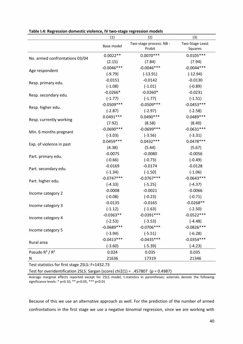
40

Table I.4: Regression domestic violence, IV two-stage regression models (1) (2) (3)

Base model Two-stage process: NB -

Probit Two-Stage Least

Squares

No. armed confrontations 03/04 0.0022** 0.0070*** 0.0105*** (2.15) (7.84) (7.94)

Age respondent -0.0046*** -0.0046*** -0.0044*** (-9.79) (-13.91) (-12.94)

Resp. primary edu. -0.0151 -0.0142 -0.0130 (-1.08) (-1.01) (-0.89)

Resp. secondary edu. -0.0266* -0.0260* -0.0231 (-1.77) (-1.77) (-1.51)

Resp. higher edu. -0.0509*** -0.0509*** -0.0453*** (-2.87) (-2.97) (-2.58)

Resp. currently working 0.0491*** 0.0490*** 0.0489*** (7.92) (8.58) (8.40)

Min. 6 months pregnant -0.0690*** -0.0699*** -0.0631*** (-3.03) (-3.56) (-3.31)

Exp. of violence in past 0.0459*** 0.0432*** 0.0478*** (4.38) (5.44) (5.67)

Part. primary edu. -0.0075 -0.0080 -0.0056 (-0.66) (-0.73) (-0.49)

Part. secondary edu. -0.0169 -0.0174 -0.0128 (-1.34) (-1.50) (-1.06)

Part. higher edu. -0.0747*** -0.0767*** -0.0643*** (-4.33) (-5.25) (-4.37)

Income category 2 -0.0008 -0.0021 -0.0066 (-0.08) (-0.23) (-0.71)

Income category 3 -0.0135 -0.0165 -0.0268** (-1.12) (-1.63) (-2.50)

Income category 4 -0.0363** -0.0391*** -0.0522*** (-2.53) (-3.53) (-4.48)

Income category 5 -0.0689*** -0.0706*** -0.0826*** (-3.94) (-5.51) (-6.28)

Rural area -0.0413*** -0.0435*** -0.0354*** (-3.60) (-5.39) (-4.23)

Pseudo R² / R² 0.024 0.035 0.035 N 21636 17319 21346 Test statistics for first stage 2SLS: F=1432.73

Test for overidentification 2SLS: Sargan (score) chi2(1) = .457807 (p = 0.4987) Average marginal effects reported except for 2SLS model; t-statistics in parentheses; asterisks denote the following significance levels: * p<0.10, ** p<0.05, *** p<0.01

Because of this we use an alternative approach as well. For the prediction of the number of armed

confrontations in the first stage we use a negative binomial regression, since we are working with

41

count data and we do not include any second stage regressors. The results of the first stage

regression are shown in Appendix A.3 in Table A.3, column 1. Here we can see that our instrumental

variables are highly significant but the pseudo R² is relatively low which indicates that the

instruments are rather weak.

The second stage regression is as in our original analysis a Probit regression. Standard errors in our

two-stage process are calculated using bootstrapping of both stages. The results are reported in

Table I.4, column 2. All models are calculated using the sample for all women. The dependent

variable is – only physical – domestic violence. Again the conflict variable increases domestic violence

and is highly significant. The weak instrument problem does however cast some doubt on the validity

of the results.

There are other potential instruments we did not use because we were not sure about the exclusion

restriction. Using them together with the elevation and oil variables increases the explanatory power

of the model used for the prediction of conflict (see columns 2 and 3 of Table A.3 in Appendix A.3),

but the R² is never very high. They are however also reported since an exploration of factors

determining the conflict intensity might be interesting. Unlike in the first stage model, we include all

Colombian districts not only the ones where interviews were conducted in these models. If no other

source is mentioned the information on the municipality indicators was obtained through SIG-OT.

The conflict is more intense in regions with higher coca production (measured as the percentage of

land in the district dedicated to growing coca plants, data from the Observatorio de Drogas de

Colombia (ODC). This is an example for economic incentives since the insurgent forces rely heavily on

income from trafficking drugs and intermediate products. If large proportions of the district surface

are covered by forest this offers cover and concealment, rest and hiding places for guerrilla troops

(forest cover data source: Food and Agriculture Organization Global Forest Resources Assessment

2000). The indicator has a positive and significant effect on conflict intensity. National highways are

interesting for all sides as lines of communication, supply and transport of personnel (or interdiction

of such). The coefficient of a dummy indicating the presence of a national highway within at least

three kilometres of the district is positive and significant. The presence of an oil refinery is

insignificant (there are only five in Colombia). Additional variables are the population density, the

presence of an oil pipeline within a distance of less than three kilometres, the distance to the next

42

larger town and to the next army base,21 indicating that conflict is actually happening closer to towns

but further away from army bases.

In general we do not see indications that the analysis suffers from an endogeneity problem, but due

to the lack of better instruments, we cannot give a definite proof for this.

I.5 Conclusion

We find evidence that the presence of intense conflict seems to increase the risk of women to be the

victim of domestic violence. We suspect the effect of conflict to work through behavioural change in

the form of higher acceptance of violence and emotional blunting, through more expressive violence

as a release for heightened stress and through higher acceptance of domestic violence by the victims

who are less willing to give up the protection of their family in an insecure environment. Our highest

estimates show an increase of more than twelve percentage points in the incidence of domestic

violence when comparing a peaceful and a conflict intensive environment which is a very large effect.

We are convinced that the effects of this change in behaviour and the long-term effect that domestic

violence has on future generations will have serious consequences for the society as a whole.

Violence from a conflict causes more violent behaviour and domestic violence affects future

generations in similar ways. This cycle of violence will then be a major hindrance for the resolution of

any conflict. The violence could also spread from the military conflict into the civil life, e.g., in the

form of different kinds of violent crime.

Colombia has a long history of violence which cannot only be seen in the conflict but also in its

enormous crime rates and the intra-family violence. It is probably a sad example of how different

forms of violence can reinforce each other. We suspect that the effect of conflict on domestic

violence is not necessarily as large in other countries as it is in Colombia. Domestic violence is always

very much influenced by the cultural and general environment and this could be more favourable in

Colombia than in other conflict regions.

We think that conflict changes attitudes and behaviour, even though as shown by Blattman (2009)

not always with only negative consequences. Understanding the impacts however is very important

for conflict and post-conflict developments. More research on the individual and behavioural effects

of conflict, especially on peoples’ attitude towards violence and its comparison across regions should

therefore prove to be very interesting areas of future research.

21 The raw data to create those indicators was extracted as Geographic Information System (GIS) data in the form of ESRI shapefiles from SIG-OT, except for the location of army bases which was determined based on information available from the web pages of the Colombian National Army. For details see Appendix A.2.

43

Chapter II: Benefits trickling away – the health impact of extending access to piped

water and sanitation in urban Yemen

Joint work22 with Stephan Klasen23, Tobias Lechtenfeld24, and Kristina Meier25

Abstract

This chapter investigates the impact of piped water supply and sanitation on health outcomes in

urban Yemen using a combination of quasi-experimental methods and results from microbiological

water tests. Variations in project roll-out allow separate identification of water and sanitation

impacts. Results indicate that access to piped water supply worsens health outcomes when water

rationing is frequent, which appears to be linked to a build-up of pollution in the network. When

water supply is continuous no clear health benefits are found compared to traditional urban water

supply through water vendors. Connections to piped sewers can lead to health improvements,

conditional on regular water supply. The findings suggest that investments in piped water supply

should not be made when availability and reliability of water cannot be guaranteed.

Keywords: Child Health, Diarrhoea, Hygiene, Impact Evaluation, Infrastructure, Sanitation, Water

Quality, Water Supply, Yemen

JEL classification: I10, I38, Q53

Acknowledgements

Together with my co-authors I would like to thank Eva Terberger, Mohammad Al-Saidi, Marlis

Sieburger, and the Evaluation Department of KfW Entwicklungsbank (Development Bank) for

valuable input. We also like to thank participants at workshops in Bonn and Frankfurt for helpful

comments on earlier versions of this chapter. Funding from the German Ministry of Economic

Development and Cooperation via KfW is gratefully acknowledged.

22 This chapter is an authors' accepted manuscript of an article published in Klasen et al. (2012), date of publication 02 Oct 2012 [copyright Taylor & Francis], available online at: http://www.tandfonline.com/ [Article DOI: http://dx.doi.org/10.1080/19439342.2012.720995]. 23 Chair of Economic Theory and Development Economics, Georg-August-University Göttingen, Platz der Göttinger Sieben 3, 37073 Göttingen, Germany, email: sklasen@uni-goettingen.de 24 Middle East and North Africa Sustainable Development Sector Department (MNSSD), The World Bank, 1818 H Street, NW Washington, DC, 20433, USA, email: tlechtenfeld@worldbank.org 25 Department Development and Security, German Institute for Economic Research (DIW), Mohrenstraße 58, 10117 Berlin, email: kmeier@diw.de

44

II.1 Introduction

Diarrhoea is one of the leading causes of child mortality in developing countries, with about 88 per

cent of death due to diarrhoea caused by poor water quality and lack of sanitation (Black, Morris and

Bryce 2003). Using cross-country observational micro data, it has been estimated that access to clean

water and adequate sanitation could prevent 2.2 million child deaths every year (Fink, Günther and

Hill 2011). However, recent impact evaluations of interventions have shown that improved water and

sanitation infrastructure, while showing positive outcomes in other dimensions, have rarely been

found to translate into better health outcomes. The reasons for this apparent lack of impact on

health have only been partially identified (Waddington and Snilstveit, 2009).

It is widely accepted that piped household connections can lead to better health outcomes than

public standpipes (Zwane and Kremer, 2007). In addition, most practitioners agree that investment in

piped water should be complemented by piped sewerage and ideally also by hygiene training to

reduce health risks from increased water use (World Bank, 2004). This is particularly important in

cities, where crowded living conditions in combination with exposed wastewater can pose serious

public health hazards. Yet, most of the empirical evidence on the health impacts of improved water

supply and sanitation in developing countries comes from rural projects, with only limited external

validity to cities.26 Very different types of water supply and sanitation are used in urban areas, where

water sources are typically found nearby, dwelling-based water access is much more common, and

water vendors deliver water to the doorstep. Urban sanitation practices also differ from villages.

Open defecation is virtually non-existent. Instead, toilets and latrines are widely used, which

discharge into open sewers, underground cesspits, or piped sanitation systems.

This chapter contributes to the evaluation literature by examining the impact of interventions to

provide piped water supply and sanitation on health outcomes in urban Yemen. It thereby

contributes to the literature by examining the impact of such schemes in water-scarce regions where

reliability of water supply can often not be assured. Yemen is a country that provides complex

challenges to project designers: Renewable water sources are extremely scarce; annual population

growth in urban areas is very high at 4.7 per cent; female education levels and general health

knowledge are low; governance structures are weak; and social conflicts regarding land and water

rights are frequent. To make matters worse, the majority of Yemen’s population of 24 million lives in

the very arid central mountains where ground water levels are rapidly falling (also due to heavy over-

26 Recent examples of rural evaluations include Rauniyar et al. (2011) on Pakistan, and Fan and Mahal (2011) on India.

45

use by agriculture) and have reached depths of up to 1000 meters. While these conditions might

seem extreme, similar environments can be found throughout the Middle East and North Africa.

The analysis uses detailed survey data from 2500 households covering treatment and control areas in

several provincial towns. The study contributes to the empirical evidence base on urban water and

sanitation access by using a mix of quasi-experimental methods which improve the robustness of the

results over a reliance on a single method (given the assumptions underlying each). These include

propensity score matching, instrumental variable regression and difference-in-difference analysis. A

second contribution is the combination of results from water tests and disease incidence data (self-

reported and facility-based). This allows a more in-depth analysis of the transmission channels from

such interventions to health outcomes.

The main results show that when piped water supply is frequently interrupted, diarrhoea among

children and adults actually increases as a result of piped water access. Additional access to piped

sanitation does not show any significant health effects in such a setting of frequent water rationing.

When piped water access is combined with reliable water flows, the negative health effects disappear

(although no positive impact is found) and piped sewerage leads to a reduction of the health burden

from water borne diseases. Additional trend analysis from secondary health facility data confirms this

picture and provides some evidence that the short-term impact may have been positive but

dissipated within a few months.

In order to identify the origins of water pollution at point-of-use, microbiological data was collected

from 9000 water quality tests covering the water chain between wells and drinking cups. The

epidemiological analysis suggests that more than half of the pollution at point-of-use comes from

unreliable water supply and possible leaks in the water pipe system. In addition, a sizable share of

water pollution can be directly attributed to unhygienic household behaviour.

The main policy message that emerges is that investment in piped water supply should not be made

when reliable water supply cannot be guaranteed.27 In such cases engaging with existing networks of

trucked water vendors or designing public standpipes might generate better health outcomes at

lower costs. In addition, the analysis suggests that rural and urban water supply and sanitation pose

different challenges. Evaluation results from rural settings are unlikely to apply.

27 See Vairavamoorthy, Gorantiwar and Mohan (2007) for an introduction to the design and control of intermittent water distribution systems.

46

The remainder of the chapter is structured as follows. Section II.2 reviews the literature on water,

sanitation and hygiene and provides a brief project description. Section II.3 introduces the data and

lays out the empirical strategy. Section II.4 discusses the impact results and investigates the origin of

water pollution. Section II.5 provides some concluding remarks.

II.2 Background

Water and sanitation projects are widely assumed to lead to substantial health improvements. This

section provides a brief review of what is known regarding the health impacts of piped water and

sanitation systems. The second part of this section presents the project under investigation and

provides details on project roll-out, selection effects, project intervention history, and explains some

relevant engineering issues.

II.2.1 Literature review

Water, Sanitation and Hygiene

Large-scale investments in water and sanitation infrastructure are typically advocated to reduce

diarrhoea and child mortality. For example, the Millennium Development Goal 10 addresses this

point by encouraging developing countries to reduce the share of people without access to improved

water and sanitation by half. The Task Force on Water and Sanitation from the related United Nations

Millennium Project asserts that massive investments would indeed help to dramatically reduce the

staggering number of 3900 children that die every day from a lack of proper water and sanitation

(Bartram et al. 2005).

This notion that piped water supply will lead to improved health is shown for Argentina by Galiani,

Gertler and Schargrodsky (2005), who investigate the impact of water utility privatization on the

incidence of child mortality by exploiting the variation of public and private ownership of water utility

across time and space. On average, the authors find reductions in urban child mortality of eight

percentage points. The impact increases more than threefold for the poorest areas of the country.

Focusing on another middle-income country Gamper-Rabindran, Khan and Timmins (2010) present

more heterogeneous findings. The marginal impact of piped water supply on infant mortality in Brazil

is the largest in areas with high initial child mortality, unless underdevelopment is excessive. Using a

quantile regression approach for panel data, the authors address a series of potential measurement

problems and unobserved heterogeneity.

This picture from Latin America is largely confirmed by a meta-analysis covering 46 peer-reviewed

studies, nearly all of them from South Asia and Sub-Saharan Africa, focusing on the health impacts of

water, sanitation, and hygiene interventions in urban and rural areas (Fewtrell et al., 2005). By

47

pooling the various results the authors find that the average intervention on water, sanitation, or

hygiene helps to reduce the relative risk of diarrhoea by somewhere between 25-37 per cent.

Importantly, water treatment at point-of-use (e.g. water boiling, use of water filters, etc.), is the most

effective intervention. The authors also caution that estimates of the impact of hygiene training (e.g.

hand washing) are likely to be overstated because they suffer from publication bias.

In direct contrast to the positive impacts of these case studies, the World Bank, in a recent review of

its activities over the past decade, concludes that it is exceptionally rare to find any health

improvements among beneficiaries of piped water schemes (World Bank, 2010). This picture is

supported by a literature review of randomized control trials by Zwane and Kremer (2007). The

authors assert that infrastructure projects in water and sanitation rarely translate into health

improvements when effective hygiene training is lacking. Inadequate water storage and handling at

the point-of-use can cripple any potential health effects from improved water sources. It is argued

that smart hygiene training is urgently needed.

Designing effective hygiene interventions has proven extremely difficult because it implies changing

habits of human behaviour. Adults are unlikely to change their hand washing practices even when

familiar with health knowledge. In addition, even if behavioural changes can be induced, they tend to

vanish soon after training, as found by Waddington and Snilstveit (2009) who review impact

evaluations from 35 countries.

The central role played by behaviour and education is also confirmed by Jalan and Ravallion (2003)

who apply propensity score matching techniques on a sample of Indian villages, where treatment

villages were connected to piped water schemes. Prevalence and duration of diarrhoea is reduced for

children living in households with piped water. However, the effect disappears when mothers have

low education and the household is very poor, which is interpreted as a proxy for inadequate hygiene

and water handling.

More explicitly, in a randomized control trial from urban Pakistan Luby et al. (2004) find that hand-

washing substantially reduces diarrhoea among children. The diarrhoea incidence among children

below 15 reduced by 53 per cent, while the duration of diarrhoea among infants reduced by 39 per

cent. Unfortunately, the follow-up study reveals that the health effect had vanished within 18

months, because treatment households stopped purchasing soap for hand-washing (Luby et al.,

2009).

This lack of sustainability is also identified by Kremer and Miguel (2007), who show in randomised

interventions at household and community level that health education does not affect behaviour.

This is not to say that information campaigns will never work, but much still needs to be understood

48

about how to alter human health related behaviour (see Dupas, 2011, for a comprehensive

introduction).

To date, no randomized studies exist that evaluate the impact of improved sanitation, such as piped

sewerage. Norman et al. (2010) provide a meta-analysis of 25 observational studies, only 16 of which

control for socio-economic differences between treatment and control groups. Nevertheless, their

review is particularly relevant, as it focuses on urban settings in which households are connected to

sewers, similar to that of the project design considered here. The estimates from the pooled meta-

analysis indicate that large reductions of up to 30 per cent of relative risk of diarrhoea incidence are

possible. While such results sound encouraging, the authors conclude that such estimates are largely

inflated and driven by non-causal research designs. More importantly, the authors point out that

sewerage networks are difficult to maintain as they require continuous water supply to avoid

clogging. Sufficient water flow can be difficult to maintain in countries with insufficient ground water

sources, which can easily jeopardize any positive health impacts of piped sanitation.

In fact, more reliable estimates of the health impact of improved sanitation tend to be much lower. A

large-scale evaluation of water supply and sanitation using panel data in Mozambique finds that

latrine use reduces the disease burden by a modest three percentage points. The overall disease

burden decreased from 30 per cent at baseline to 27 per cent after the intervention (Elbers, Gunning

and Vigh, 2012).

Overall, the impact of water and sanitation projects seems to be unclear. Most randomized and

quasi-randomized studies lead to the conclusion that water and sanitation interventions can be

expected to achieve their health targets if households use hygienic practices for storage and handling

of drinking water (see for example Clasen et al., 2007, Curtis and Cairncross, 2003, or Gundry, Wright

and Conroy, 2004). How to best achieve and sustain such behaviour among poor households has yet

to be shown and appears to be highly context specific (Waddington and Snilstveit, 2009).

The secondary effects from water and sanitation largely depend on positive health impacts. They

include lower health care cost and increases in labour productivity and school attendance (Poulos et

al., 2006). In addition, access to piped water can lead to reduced water costs and increases in

consumed water quantity. On the negative side, it is possible that in traditional societies piped

household connections reduce the time women spend outside the house, with potentially

detrimental effects on their social capital and learning through peers (Janssens, 2011). While the

research design of this evaluation addressed all these issues, no impacts were found regarding such

secondary effects.

49

II.2.2 Project description

More than two thirds of Yemen’s population of 24 million lives in the rugged central highlands that

range between 2000 and 3200 meters. Rainfall is rare and erratic and most people live from farming

crops on small terraces on steep cliffs. The rest of the population lives in the desert-like coastal plain

that stretches along the Red Sea in the west, and in small towns and hamlets on the southern coast.

Very few people live in the eastern half of Yemen in what is commonly referred to as the ‘Empty

Quarter’. The urban population is largely engaged in local trade, the service sector or employed by

the public sector.

The northern part of Yemen, which today comprises nearly 85 per cent of the population, only

emerged from total isolation in 1970. Under the Imamite, modern water and sewerage networks,

electricity and telephone grids, cars and many other technological innovations had been banned.

Piped water supply is still lacking today in many urban areas, forcing families to primarily rely on

water vendors who fill their tanks at agricultural wells outside the city. Very few wealthy families can

afford to drill and operate their own borehole, especially in the mountains where the water table is

several hundred meters deep.

The Provincial Towns Program (PTOP), a program of the Yemen government with partial support by

German Financial Cooperation (by the development bank branch of the Kreditanstalt für

Wiederaufbau, KfW) to improve urban water supply and sewage systems in Yemen, was designed to

drill new wells in eight provincial towns, located along the southern and western coast and in the

central mountains. Wells were equipped with pump stations and water treatment facilities which are

operated by independent public water utility companies. Piped water schemes were designed to

connect all existing households and have the capacity for future expansion. As the program led to an

increase in water use it brought the existing waste water systems – consisting of underground

cesspits and open sewers – to the verge of collapse. In response, sewerage schemes and wastewater

treatment plants were constructed. They connect a large share of households with access to piped

water to a sanitation network which allows wastewater to flow through sewerage pipes to a

wastewater treatment plant.

For the impact evaluation two locations were selected by the research team based on five criteria.

First, the town needed to be large enough to draw a sizeable sample. Second, a preference was given

to towns in which connections to water or sewage systems were not universal in order to create in-

town control groups that could be used during analysis to control for unobserved town effects. Third,

the two towns were chosen to resemble the main topographic characteristics of Yemen. Fourth,

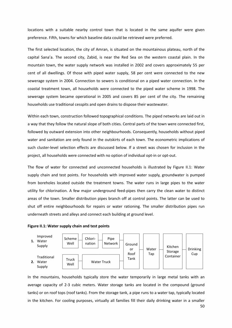
50

locations with a suitable nearby control town that is located in the same aquifer were given

preference. Fifth, towns for which baseline data could be retrieved were preferred.

The first selected location, the city of Amran, is situated on the mountainous plateau, north of the

capital Sana’a. The second city, Zabid, is near the Red Sea on the western coastal plain. In the

mountain town, the water supply network was installed in 2002 and covers approximately 55 per

cent of all dwellings. Of those with piped water supply, 58 per cent were connected to the new

sewerage system in 2004. Connection to sewers is conditional on a piped water connection. In the

coastal treatment town, all households were connected to the piped water scheme in 1998. The

sewerage system became operational in 2005 and covers 85 per cent of the city. The remaining

households use traditional cesspits and open drains to dispose their wastewater.

Within each town, construction followed topographical conditions. The piped networks are laid out in

a way that they follow the natural slope of both cities. Central parts of the town were connected first,

followed by outward extension into other neighbourhoods. Consequently, households without piped

water and sanitation are only found in the outskirts of each town. The econometric implications of

such cluster-level selection effects are discussed below. If a street was chosen for inclusion in the

project, all households were connected with no option of individual opt-in or opt-out.

The flow of water for connected and unconnected households is illustrated by Figure II.1: Water

supply chain and test points. For households with improved water supply, groundwater is pumped

from boreholes located outside the treatment towns. The water runs in large pipes to the water

utility for chlorination. A few major underground feed-pipes then carry the clean water to distinct

areas of the town. Smaller distribution pipes branch off at control points. The latter can be used to

shut off entire neighbourhoods for repairs or water rationing. The smaller distribution pipes run

underneath streets and alleys and connect each building at ground level.

Figure II.1: Water supply chain and test points

1.

Improved Water Supply

Scheme Well

Chlori-nation

Pipe Network

Ground

or Roof Tank

Water Tap

Kitchen Storage

Container

Drinking Cup

2.

Traditional Water Supply

Truck Well

Water Truck

In the mountains, households typically store the water temporarily in large metal tanks with an

average capacity of 2-3 cubic meters. Water storage tanks are located in the compound (ground

tanks) or on roof tops (roof tanks). From the storage tank, a pipe runs to a water tap, typically located

in the kitchen. For cooling purposes, virtually all families fill their daily drinking water in a smaller

51

kitchen storage container every morning, which holds 10 to 20 litres. For drinking, many families

share a single cup when drinking from the kitchen storage container.

In areas where no piped water is available, drinking water is purchased from water vendors using

water trucks (mountainous region) or donkey carts (coastal region). Water vendors obtain their water

from agricultural wells outside the town. Truck water is directly pumped into the water storage tank.

It is also purchased by connected households during extended periods of water rationing.

II.3 Data and empirical strategy

II.3.1 Data

This chapter uses an array of data sources, combining household survey data, microbiological water

test results and secondary data from schools and health facilities.28

Household Sample

The household survey was conducted in the four treatment and control towns in the second half of

2009, covering 2518 randomly selected households. The sampling frame is based on an innovative

remote aerial mapping approach using satellite images, where each rooftop is assigned a building

identification number. The sample is then drawn from this building inventory. This is done by dividing

each town into equally spaced clusters, all of which entered the sample to ensure representative

coverage of all urban neighbourhoods. Households within each cluster are drawn following a

stepwise procedure beginning from a random starting point. In these provincial towns, very few

buildings are home to more than one family. In such cases, an additional sampling-procedure allowed

field supervisors to select a random household for the interview. Overall, sampling based on satellite

images facilitates field work, since interviewers can use detailed street maps where selected houses

are marked. Even in small alleys exact locations can be confirmed using Global Positioning System

(GPS) coordinates. In the absence of recent reliable and available census data, such an approach is

the best available alternative to ensure proper sampling.

A cross-sectional baseline survey exists from 2004 for the mountain town of Amran that was used to

ex-ante evaluate the feasibility of the intervention. The baseline instrument contains questions on

education, health, and demographic structure which were replicated in the endline survey to allow

the calculation of double differences.

28 The questionnaires used to collect data in the main household survey, the water test supplementary survey, and at education and health facilities are provided in English language in the appendices of Klasen et al. (2011).

52

Outcome Variables

Following best-practice in survey design, the household interviews collected information on

symptoms rather than diseases. In environments with poor health knowledge, limited access to well-

equipped health facilities and existing folk medicine, self-reported symptoms are much more reliable.

A useful categorization of water borne diseases and transmission channels has been compiled by

Esrey et al. (1991), on which the list of symptoms was developed and tested with medical personnel

from Yemen.

Diarrhoea is the principle predictor of water borne diseases. Secondary symptoms include vomiting,

abdominal pain and fever which are combined with data on the incidence of watery and bloody

diarrhoea (dysentery) to create an overall disease measure for robustness analysis. Additional

outcomes are school and work days missed due to water-related symptoms. Analysis takes place at

the household level, using morbidity rates within each household. The Severity indicates the share of

reported symptoms classified as severe. Since disease incidence among small children is a crucial

impact indicator, the variables Disease, Diarrhoea and Severity are also included for the subgroup of

children up to the age of five.29

Main Covariates

In line with existing empirical literature, a set of household characteristics is included in the analysis

to control for differences in hygienic practices, education, wealth, and demographic structure.

Education, hand washing, soap use, water purification (incl. the use of water filters, chlorination and

boiling), and knowledge about water-related diseases are expected to reduce the relative disease

burden. Respondents were also asked about problems with water supply, water quality and the

sewerage system, which are expected to be negatively associated with health. The demographic

structure of the household might also affect the disease burden. Infants and young children are prone

to water borne diseases given their weak immune system. In addition, illnesses spread fast within

households, putting more people at risk in larger households.

Wealth is an important control for unobserved health practices. At the same time, perceived health

status is typically negatively correlated with income which could create a reporting bias among the

better-off and is important to be controlled for. House owners are expected to invest more into water

tanks and pipes and are exposed to reduced health risks.

29 For a full list of variables see Appendix B.1.

53

Water Test Data

To supplement survey data on subjective water quality with hard evidence, water tests were

conducted using physical, chemical, and microbiological indicators.30 While water pollution can have

many origins, this study focuses on Escherichia coli (e.coli), a bacterium that is associated with human

faeces. E.coli directly causes dysentery, sometimes referred to as bloody diarrhoea, and is a common

indicator for health studies in the developing world. It is easily detectable in water samples and there

is at most incomplete resistance as a result of continued exposure.

Water tests were conducted along the water supply chain of a random subsample of 500 households

after the main household survey was completed. Additional interviews with well owners, water

vendors and household members complemented the tests.

Health Facility Data

Data on diagnosed illness was collected on a monthly basis spanning twelve years from 1998 to 2009.

Based on inpatients and outpatients registration books with information on diagnosis and

prescription, the incidence of several water-related diseases was aggregated, including diarrhoea.31

Because of data gaps and changes in official coding, diarrhoea data can be used from 2004 to 2009

for the mountain towns. This covers the period from just before the sanitation intervention until the

endline survey. For the coastal towns, trends can only be compared between 2008 and 2010 which is

ex-post for water and sanitation. Health facility data are coded as monthly stock variables and are

logged and deseasoned for analysis. Only diarrhoea incidence is used for analysis given data gaps in

the other indicators.

II.3.2 Empirical strategy

The empirical strategy does not rely on a single preferred method or result. Instead, a wide array of

quasi-experimental approaches is used to identify robust relations between treatment and health

outcomes. This is necessary because access to piped water and sanitation is purposively assigned to

entire neighbourhoods and streets, given the enormous financial inefficiencies that would result from

randomized treatment. In effect, systematic differences between treatment and control areas might

30 Physical indicators are Electrical Conductivity, Total Dissolved Solids and pH Value. Chemical indicators are Hardness; and content of Calcium, Chloride, Total Iron and Fluoride (only measured at source) and Nitrate and Sulphate (measured at source and point-of-use). Biological indicators are contamination with e.coli and Total Coliform. 31 The water-related diseases are bilharzias (intestinal and urinary) and schistosomiasis, amoebic dysentery and giardia, diarrhoea, hepatitis A, typhoid, malaria and intestinal worms (including flukes, hookworm, pinworm, roundworm, tapeworms, whipworm, and others).

54

exist which can influence the success of the intervention. To illustrate this crucial point, consider a

simple impact model

𝑦𝑖 = 𝛼 + 𝑥𝑖′𝛽 + 𝑇𝑖𝛾 + 𝜀𝑖 (II.1)

where 𝑦𝑖 denotes the outcome (e.g. diarrhoea) for observation i, 𝑥𝑖′ is a vector of covariates, 𝛽 is a

vector of parameters, Ti is a variable indicating treatment, and 𝜀𝑖 is an idiosyncratic error term, with

ε~ N(0,σ2). In the case of non-random assignment of treatment T, Cov(T, ε) ≠ 0, which biases 𝛾,

the estimated impact of treatment. The possibility of selection bias is addressed using propensity

score matching and instrumental variables regressions on cross-sectional survey data. Difference-in-

difference impact estimates are also presented using the baseline data.

Propensity Score Matching

In all Propensity Score Matching (PSM) procedures, treatment and control households are matched

on their predicted probability of being part of the treatment group (Rosenbaum, Rubin 1983

Rosenbaum and Rubin, 1983). The model used to estimate the propensity score should include all

covariates that determine treatment without being affected by treatment themselves. The propensity

score model used here includes the education level of the household head, household size,

dependency ratio, house ownership, and an indicator for knowledge of water-related diseases.32

Since PSM is limited to observable characteristics results may still be biased if the selection of the

treatment group was driven by unobservables. Usually one would presume that such a bias would

overestimate positive effects of an intervention to the extent that neighbourhoods selected for

treatment might have unobserved favourable characteristics that would lower their disease

incidence.

Instrumental Variables

The instrumental variable (IV) approach is a complementing alternative of dealing with potential

selection bias when such bias is due to unobservables. The impact is calculated from the predicted

treatment status 𝑇�𝑖, which is estimated by a set of instrumental variables that are not correlated with

the error term 𝜀𝑖; and which may not affect the outcome variable directly.

The instruments used here are based on project documents and in-depth interviews with

stakeholders. The construction of water and sanitation schemes followed three principles which can

be exploited as instruments. First, construction always began in the city centre. Second, the Old City

32 A large set of alternative model specifications was tried, including the use of geographical conditions (distance to city centre, rocky ground), age of house, and other socio-economic variables, none of which improved performance of the propensity score model.

55

was prioritized, where buildings are substantially older. Third, in the mountain region pipe

construction excluded streets built on particularly hard rock due to increased construction cost.

Suitable instruments are therefore Distance to the City Centre of each household, the Age of the

House and Rocky Ground around the dwelling, all of which perform well with regard to first stage F-

tests33 and Hansen tests. While these instruments are useful when quantifying the impact using the

in-town control group, an additional binary instrument taking the value of one for the Project Town is

included when the sample contains both in-town and out-town control groups in order to allow for

unobserved differences between the control groups.

Double Differencing

Double Differencing (DD) is an alternative for identifying causal effects when baseline data is available

and no time-variant unobservable confounders have affected the outcome. The analysis is done using

mean point estimates from two cross sectional surveys, which accounts for differences in sample size.

Since sanitation is only provided to a sub-sample of the water treatment group, which can be used to

quantify the relative sanitation impact, by taking the additional difference between the double

difference results of piped water and access to piped sewerage. This DD analysis can only be done for

Amran as the baseline survey is only available for that town. Questions for eliciting the disease

burden are identical in the baseline and endline survey instruments. However, even in case of

differences in measurement, DD results would be unbiased because the disparities would cancel out.

Trend Analysis using Health Facility Data

Moving averages are used to estimate trends of between-town differences in waterborne disease

burden. Unfortunately, within-town comparisons are not possible because record books of health

facilities do not contain full addresses but only city of origin of patients. For the mountain towns, the

available data allow an investigation of the sanitation intervention. For the coastal towns, trends can

only be compared over the three years prior to the endline survey when all interventions had long

been completed. This provides an interesting opportunity for investigating long term effects by using

information on converging or diverging trends.

Potential Caveats

Health outcomes such as diarrhoea incidence are self-reported and might be biased for two reasons.

First, poorer people tend to underreport the disease burden of very common illnesses, which can

make wealthier cohorts look worse off. Second, health knowledge may be limited among less

33 The only exception is the F-test for the analysis of sanitation in the coastal town, which is always well below critical reference values recommended by Stock and Yogo (2005). This means that results there have to be interpreted with caution.

56

educated cohorts and hence symptoms underreported. While it cannot be excluded that such

measurement bias affects the survey data, relative comparisons between treatment and control

groups will be unbiased when measurement error affects both groups in a similar way. Nevertheless,

a wealth indicator is used in the analysis to directly control for measurement bias.

Externalities of water and health related interventions have been shown for rural setting (Miguel and

Kremer, 2004). In the case of benefit spillovers to the control group the econometric identification of

the causal impact would be invalid. This could be the case if the risk of water-borne diseases such as

cholera is reduced for the entire urban population even though only part of the population is

connected to improved water sources. It might also happen if the use of piped sanitation by part of

the populations reduces the risk of overflow of open sewers among unconnected households along

with a reduction in health risk. In such situations the health outcomes of the control population

would increase due to the project. Since the impact estimates rely on the differences in health

outcomes, the estimates would be biased downwards. The use of control towns addresses this

problem. Since control towns are located at a distance of 10 to 20 kilometres from treatment towns,

externalities affecting health risk can be excluded.

II.4 Results

This section begins with the results from the quasi experimental impact estimation. The second part

of this section discusses possible causes of water pollution between water source and point-of-use to

explain the limited health impact of the intervention.

II.4.1 Project impact

a. Evidence from the descriptive analysis

The descriptive analysis of disease incidence among treatment and control groups reveals an a priori

unexpected picture in Table II.1. Connection to piped water is associated with a higher disease

burden in both the mountains (Amran) as well as the coast (Zabid). At the same time, households

connected to the scheme in Amran complain about substantial rationing, where no water is available

60 per cent of the time. As a result, more than 25 per cent of treatment households did not use any

piped water in the 90 day reference period. In comparison, no rationing is reported in the coastal

treatment area, and consequently all surveyed households used only piped water in the reference

period. Among mountain households with access to piped water and sanitation, about 11 per cent of

household members reported water-related symptoms during the past month. For children aged zero

to five this share is four times higher, and such higher disease incidence among treated households

also carries over to the severe disease indicators. In the coastal treatment town, the disease burden is

more pronounced among households with access to piped water only, while the additional access to

57

sanitation for those households appears to reduce disease incidence. Regarding secondary effects

(workdays or schooldays missed), there are no clear patterns; if anything more work- and schooldays

are missed in treatment than control households.

Table II.1: Disease burden among household members

Indicator

Dise

ase

Dise

ase

(chi

ld)

Diar

rhoe

a

Diar

rhoe

a (c

hild

)

Seve

rity

Seve

rity

(chi

ld)

Wor

kday

s m

issed

Sc

hool

days

m

issed

Hous

ehol

ds

Region Connection Mean prevalence among applicable household members N

Mountainous

Water 9.9 30.2 5.3 13.8 7.6 34.8 0.9 0.3 201 Water & Sanitation 11.2 46.8 5.8 15.9 8 44.3 6.4 1.4 270 None 8.2 25.8 3.4 9.8 6.1 27.6 1.8 0.2 374 Control 6 20.5 3.3 4.9 5 21.8 2.3 0.1 298

Coastal Water 11.2 37.1 5.1 11.8 6.6 37.6 1.3 5.4 127 Water & Sanitation 7.2 26.1 3.5 10.6 4.7 29.1 1.6 1.4 714 Control 6.4 21.9 3.3 8.2 4.3 17.9 1.8 1.2 434

Total 7.9 28 3.9 10.2 5.6 28.7 2.2 1.2 2418 Note that in the coastal treatment town there is no in-town control group (“None”) available.

b. Evidence from propensity score matching

Water

Table II.2 shows the matching results for access to piped water.34 The first two columns show the

results for the between-town analysis by region. The results suggest sizable and significant increases

in disease burden among mountain households connected to piped water. Children in particular are

affected by an increase of diarrhoea incidence of nearly ten percentage points. The picture is

confirmed by the severity of diarrhoea among children and by the aggregate measure of five

waterborne diseases. The effect remains significant for the aggregate waterborne disease incidence

and its severity for all age groups, implying a widespread increase in illnesses in the population. In the

coastal region, between-town matching shows an increase in total disease incidence by about four

percentage points among households with access to piped water; but results for the other disease

indicators are insignificant. In addition, the number of missed school days seems to have slightly

increased among school-aged children.

The third group of columns in Table II.2 contains the findings of within-town matching in the

mountain region. Again, adverse health effects of piped water are found, albeit with somewhat lower

34 Results are reported for radius matching using a calliper of 0.05. Similar results are obtained when applying smaller or larger callipers, nearest neighbour matching, and kernel matching using a Gaussian kernel with different bandwidths. Refer to the appendix of Klasen et al. (2011) for a more complete overview of these results.

58

magnitude, especially for children up to five years of age. Recall that drinking water quality cannot be

included in the propensity model, because it is directly affected by treatment. Given that part of the

treatment group regularly uses traditional water sources during periods of water rationing, i.e. the

same water as the in-town control group, the negative health impact from the in-town matching is a

conservative estimate and possibly underestimated.35

Table II.2: Propensity score matching – impact of water

Outcome

Coastal Region Mountainous Region

out-of-town control out-of-town control in-town control

ATT t-value N ATT t-

value N ATT t-value N

Disease 0.0399** 1.98 560 0.0455*** 2.76 488 0.0268* 1.72 567 Diarrhoea 0.0111 0.73 560 0.0193 1.53 488 0.0195* 1.75 567 Severity 0.0184 1.21 560 0.0329** 2.25 488 0.0239* 1.76 567 Workdays missed -0.0074 -0.59 560 -0.0076 -0.6 496 -0.003 -0.19 573

Schooldays missed 0.0441* 1.81 560 0.0018 0.84 496 0.0018 0.57 573

Disease (child) 0.1328 1.36 338 0.1078* 1.71 361 0.0631 1.17 409 Diarrhoea (child) 0.0151 0.38 338 0.0954*** 3.19 361 0.0412 1.3 409 Severity (child) 0.1879 1.62 338 0.1347* 1.87 361 0.1041 1.63 409

Note: To analyse the impact of piped water supply only, the treatment group excludes households with access to the sewerage system. For the between-town calculations only out-town control groups are used. Matching with the in-town control group is only possible in the mountainous region. ATT indicates the Average Treatment effect on the Treated.

Sanitation

Since improved sanitation is conditional on access to piped water, the impact of sanitation in Table

II.3 is estimated by matching households from the water group (controls) to households from the

water and sanitation group (treatment). Estimates need to be interpreted relative to the impact of

piped water.

In the mountain town, additional negative health effects are found for children. The difference

between the matched treatment and control groups is nearly 14 percentage points. These

detrimental health outcomes lead to a significant increase of days that children miss school due to

waterborne diseases. The effect for missed work days is also significant. For the coastal town, no

health effect is found for children or health related absenteeism. Interestingly, a slight reduction of

the disease incidence of almost four percentage points is found for the overall population.

35 In theory, positive health externalities of piped water might be an alternative explanation for the more similar health outcomes within the mountain project town. They are not very likely, given that health outcomes are in fact worse among the treatment group.

59

Table II.3: Propensity score matching – impact of sanitation

Outcome

Coastal Region Mountainous Region

out-of-town control out-of-town control

ATT t-value N ATT t-value N

Disease -0.0373* -1.79 841 0.0187 0.99 458 Diarrhoea -0.0207 -1.3 841 0.0087 0.62 458 Severity -0.0244 -1.53 841 0.0077 0.48 458 Workdays missed 0.0086 0.78 841 0.0567* 1.87 469 Schooldays missed -0.0346 -1.32 841 0.0097* 1.75 469 Disease (child) -0.1172 -1.03 418 0.1382* 1.73 327 Diarrhoea (child) -0.0223 -0.51 418 0.015 0.4 327 Severity (child) -0.0899 -0.64 418 0.0684 0.84 327

Water rationing – which is common in the mountain town – could be the transmission channel for the

additional disease burden from the sewerage scheme. The probable reason is that without regular

water flow, sewers are prone to clogging.

c. Evidence from instrumental variable regressions

Water

The IV results for access to piped water are summarized in Table II.4 (see full results in Appendix B.3).

Specification tests suggest the validity of the instruments. The results are very similar to the matching

estimates.36 Access to water supply in the mountain town is associated with a higher disease burden

for children and adults. Again, the magnitude of the impact is larger for children.

The covariates of the IV regressions shed some light on the transmission channel of the observed

negative impact. Access to Sanitation is insignificant in all specifications, suggesting that a connection

to piped sewers does not have sizable health effects in this project. The positive and significant effect

of Trucked Water used by connected households indicates that illnesses are partly caused by

contaminated water purchased from tanker trucks. No effect is found for Water Purification, probably

due to the surprisingly small number of households engaging in water treatment at point-of-use.

Among the socio-economic factors, the most influential variables are House Ownership which reduces

36 As already mentioned in the methodology section, a dummy variable indicating location in Amran is included as an additional instrument in the analysis. As a robustness check, the analysis is repeated without the dummy, using only the in-town control group for water in Amran. Results were very similar in magnitude, although some of the coefficients were no longer significant (also due to the much smaller sample size). Nevertheless, the general conclusion of a negative effect of piped water on health remains clearly visible and is significant for several of the disease indicators.

60

disease incidence, and the Share of Children and Elderly living in the household which increases the

disease incidence. These effects are consistent in both regions.

Table II.4: Instrumental variable analysis – impact of water Outcome Mountains

Water Impact F-test First Stage

Hansen p-value N

Disease 0.0723** 78.71 0.561 1072

Diarrhoea 0.035 78.71 0.380 1072

Severity 0.0669** 78.71 0.294 1072

Disease (child) 0.213* 57.76 0.795 784

Diarrhoea (child) 0.155*** 57.76 0.645 784

Severity (child) 0.307** 57.76 0.557 784

Note: The sanitation indicator is included as an additional covariate in the analysis to allow the use of the full sample. There is no in-town control group for water in Zabid, as all households are connected to piped water, which is why the analysis cannot be meaningfully performed for the coastal region.

Sanitation

The results for sanitation in the mountain area do not show significant positive or negative effects for

any of the outcome variables or age groups (Table II.5). Estimates for the coastal region cannot be

meaningfully interpreted as we have a weak instrument problem. This could explain why IV results

are not significant with regard to sanitation, despite the coefficients having the same direction as the

matching results.37

Table II.5: Instrumental variable analysis – impact of sanitation Outcome Mountains Coastal

Sanitation Impact F-test First

Stage

Hansen p-value N Impact

F-test First

Stage

Hansen p-value N

Disease 0.008 46.91 0.887 436 -0.152 3.16 0.330 826

Diarrhoea 0.011 46.91 0.335 436 -0.071 3.16 0.420 826

Severity 0.024 46.91 0.518 436 -0.079 3.16 0.792 826

Disease (child) 0.103 34.38 0.907 311 -0.552 4.938 0.703 411 Diarrhoea (child) 0.001 34.38 0.632 311 -0.187 4.938 0.496 411

Severity (child) 0.158 34.38 0.667 311 -0.626 4.938 0.793 411

37 Values of the first stage F-test are below critical reference values recommended by Stock and Yogo (2005).

61

Overall, propensity score matching and instrumental regressions generate very similar results. Water

access appears to have increased health problems in the mountain town where water rationing is

frequent, with access to sanitation aggravating the unintended health consequences even further. In

turn, no health improvements are found in the coastal town related to piped water supply, while

piped sewers are associated with a reduced disease burden.

d. Evidence from double difference calculations

Analysis using cross-sectional survey data from before and after the water and sanitation project

confirms the above results. Table II.6 shows the disease burden for diarrhoea among all age groups,

which has increased by 1.37 percentage points in the mountain town among households connected

to piped water.38 This is considerably less than the matching and IV estimates, because it is relative to

the previous water supply scheme that was replaced by the project. At baseline, a water pipe scheme

existed of abysmal quality. In fact, it was so inadequate und unreliable that the city qualified for

participating in the project to upgrade its water supply network. The old water system is very likely to

have posed serious health threats to the connected population.

Table II.6: Double difference results for water and sanitation

Mountains Diarrhoea Baseline Endline

Percentage Points Individuals Individuals

First Difference: change over time Water 3.44 1744 1832 Sanitation 4.35 1744 2256 Control 2.07 1118 2922

Double Difference: treatment – control Water 1.37 Impact of Water Sanitation 2.27

Treatment Difference 0.91 Impact of Sanitation

Access to sanitation is conditional on access to water. By splitting the sample of households

connected to water in two groups defined by access to sanitation, the difference between treatments

can be obtained, yielding impact of sanitation in addition to water. Estimates for the mountain town

38 Results are point estimates based on two cross sectional surveys covering the entire city at baseline and endline. T-tests indicate that these results are significant at conventional levels. To exclude possible confounding effects from population growth the analysis is also done with a restricted endline sample that only includes neighbourhoods surveyed at the time of baseline, which does not yield very different results. Analysis cannot be performed for the coastal region because no in-town control group for water exists at the endline.

62

imply an additional increase of diarrheal disease incidence by 0.91 percentage points when

households are connected to piped sewerage.

e. Evidence from health facility data

To complement the health impacts from self-reported health, secondary data from health facilities is

analysed which contains the monthly diarrhoea incidence. Figure II.2 shows relative diarrhoea

incidence between treatment and control towns for each region for children.

For the mountain region, the relative disease burden in the treatment town increases sharply for

children during the first year after project completion (see the low starting level in 2004, when

treatment households were connected to sanitation).39 Unfortunately, limited data availability means

that no ex-ante trend can be established to further analyse why the disease burden worsened over

time.

Figure II.2: Differences in diarrhoea incidence between treatment and control towns

The trends level off after a few months, but remain on a much higher level than in the control town.

The effect is very pronounced and remains visible even though in-town control households with a

lower reported disease burden were also visiting the health facilities of the treatment town.40 For the

coastal region, the estimated trend of the relative disease burden is increasing over time in the

treatment town, although the variance is quite large. Since the sanitation and water projects have

been completed before 2008, the figure only provides a snap-shot of a medium-term impact. But

these data clearly are consistent with our other analyses that suggest that extension of water and

39 In principle, the same result can be caused by a major outbreak of waterborne diseases in the control town, e.g. cholera. However, the control town health data do not show a surge in diarrheal diseases in the first half of 2004 but rather a decline. 40 Since reported health status is similar among control groups inside and outside of treatment towns the possibility of in-town control households driving the results can be excluded.

.51

1.5

22.

53

ln(tr

eatm

ent)

- ln(

cont

rol)

2004m1 2006m1 2008m1 2010m1Year

Children 0-5 years - Mountain Region

.1.2

.3.4

.5.6

ln(tr

eatm

ent)

- ln(

cont

rol)

2008m1 2008m7 2009m1 2009m7 2010m1Year

Children 0-5 years - Coastal Region

63

sanitation access did not improve health outcomes, but appears to be associated with a worsening of

health outcomes in treatment towns.

II.4.2 Sources of water pollution

The objective of the Provincial Towns Program was to improve the health situation of the population

by providing access to safe drinking water and an effective sanitation infrastructure. The impact

results show that health did not generally improve from the investments in water and sanitation.

Only in the coastal town marginal reductions in disease burden was achieved for households

additionally connected to sanitation. This raises the question about causes of water pollution in

households connected to piped water.

Microbiological tests reveal that water pollution at point-of-use is rampant in treatment and control

areas (see Table B.3 and Table B.4 in Appendix B.2). In the mountains, e.coli was detected inside the

drinking cup of 20.0 per cent of households only connected to piped water. Virtually the same

incidence (20.3 per cent) is found among control households using traditional water sources. This

implies that the water scheme made no difference to water quality at point-of-use. Worse, e.coli

incidence among households that are additionally connected to sewers is at a staggering 38.4 per

cent. This is very similar to the e.coli incidence in the mountain control town without any water or

sanitation facilities (40.0 per cent). In the coastal area, water pollution at point-of-use is even higher,

affecting 46.6 per cent of all households connected to piped water and 36.6 per cent of households

connected to water and sanitation.

Two major channels for water pollution exist that could help explain these findings. First, the piped

network might be a source of pollution, for instance through broken pipes, insufficient chlorination,

and frequent water rationing. Second, unhygienic household behaviour when storing and handling

water might be an additional cause.

a. Pollution from the pipe system

Following the water from the well to the household, several sources of contamination are possible.

First, no signs of pollution are found in any of the wells of the water schemes. Second, in the coastal

town one of the two main water pipes running into the town was tested positive for e.coli pollution,

which indicates leaks in that pipe. The main pipes in the mountains were clean. Third, leaks in the

small distribution pipes might cause additional pollution, which leads to streets with an above

average pollution level. As shown graphically in Figure B.1 in Appendix B.4, two close-to-linear

patterns – in parts coinciding with such streets – appear to be identified for the coastal town of Zabid,

implying wastewater intrusion into the drinking water system.

64

b. Pollution from water storage tanks

Most households store drinking water in large tanks which could be a source of pollution. Descriptive

analysis suggests that water tanks are not related to water pollution. This includes the existence of a

water tank, the size of the tanks, the storage time of water in the tanks, and the location of the tank

(roof versus ground). In addition, none of the surveyed households is trying to reduce pollution in

their tank by adding chorine or other methods, or has cleaned the inside of their tank in the twelve

months prior to the interview. In effect, water tanks do not help explain any differences in water

pollution at point-of-use. Since tanks are closed and out of reach of humans, e.coli pollution found

inside the tanks must come from the pipe network or from truck water pumped into the tanks.

c. Pollution from water rationing

The impact estimates show a negative effect from piped water in the mountain town, which suggests

a mechanism of water pollution not found in the coastal town. Since pollution of the main pipes can

be ruled out, the remaining suspect is irregular water supply. Such water rationing is found in all

neighbourhoods of the mountain town but is only reported by a fraction of the coastal households.

Interviews with the engineers of the water utility confirm that water availability is very irregular in

the mountains since three out of five source wells have fallen dry shortly after project inauguration.

The resulting water flow is insufficient to provide permanent drinking water for the entire town.

Consequently, water is only available on a few days per week in each neighbourhood.

Epidemiological literature has shown that water rationing itself can be a serious cause of pollution

through three channels (see Le Chevallier, Friedman et al., 2003, for an introduction to the topic and

Semenza et al., 1998, for an excellent empirical contribution from an urban setting). First, during

periods of rationing, microfilm grows in the pipes and is flushed out through household connections

when water pressure resumes. Second, without reflux valves, water schemes are prone to pollution

reversely entering from water taps, when falling water pressure sucks in any residues. Third, given the

change in water pressure, even minor pipe leaks can cause pollution of the piped water during

rationing. This is especially important where water pipes run nearby underground cesspits, which is

reportedly very common in urban Yemen.

In addition, extended periods of water rationing cause connected households to refer to traditional

water sources. Pollution in the tanks could thus stem from households using a mix of improved and

traditional sources. In fact, controlling for the mixing of water sources during the past four weeks

helps to explain about half of the e.coli pollution in water storage tanks. This source of pollution is a

direct consequence of water rationing. The remainder of the e.coli pollution inside the tanks is, by

implication directly caused by pollution in the pipes.

65

d. Pollution from household behaviour

Lastly, it is well established that lack of hand washing and other unhygienic household behaviour can

adversely affect water quality at point-of-use (Jensen et al., 2002). Compared to water pollution at

the tap, e.coli incidence increases towards the drinking cup. The average change in e.coli incidence

within the household is 24.1 percentage points from the storage container to the drinking cup with

very little variation between treatment and control areas (see Table B.4 in Appendix B.2). In other

words, at least a quarter of all households suffer from pollution caused by their own behaviour.

Overall, this section shows that water pollution is rampant in both treatment and control areas. In the

treatment group e.coli incidence averages 35.4 per cent at the point-of-use. By investigating the

pollution at different locations along the water chain, more than half of the overall pollution is found

to be due to leaking pipes and water rationing. The remainder of e.coli pollution can be directly

attributed to household behaviour.

II.5 Conclusion

Lacking access to clean drinking water and improved sanitation is the largest cause of child mortality

in the developing world and responsible for a large share of the global disease burden. Increasing the

number of people with access to improved water and sanitation is therefore a priority among policy

makers. Massive investments in piped infrastructure for water and sewerage are common and are

expected to decrease the risk of diarrhoea among beneficiaries. Although the evidence is mixed, a

significant impact on health outcomes is rarely identified. According to a vast literature, this is

primarily due to unhygienic household behaviour which causes pollution at the point-of-use. Effective

methods on how to sustainably alter behaviour have not yet been identified.

This study quantifies the health impacts from a large scale water and sanitation project in urban

Yemen. Health outcomes include diarrhoea among children and adults, and several health related

factors, including school and work-place attendance. By exploiting differences in the roll out of

project components, the impact for water and sanitation can be analysed separately.

Using a range of quasi-experimental methods on survey data from treatment and control towns, we

find that the overall health impact of the infrastructure investment is mixed, at best. In the mountain

town of Amran, health has deteriorated for households connected to the water scheme. The

existence of piped sewerage has no significant health effects. For the coastal town of Zabid, no clear

effects are found for piped water supply. Additional access to sewers seems to marginally improve

the water- borne health burden.

66

To explain these results, microbiological water tests were conducted on several points between the

wells (water source) and the drinking cups within a sample of households (point-of-use). Water

pollution is extremely high in treatment and control areas. The average incidence of e.coli at the

point-of-use is 35.4 per cent for treatment households, while the water source is found to be clean.

When dividing the pollution between piped scheme and household behaviour, more than half of the

total pollution is found to come from leaking pipes and water rationing. The remainder of e.coli

pollution can be attributed to household behaviour. These results are likely to apply to water and

sanitation projects in many urban settings characterized by water scarcity and fast population growth

in the Middle East, North Africa, and elsewhere in the developing world.

Five policy implications emerge from this study. First, water networks should only be extended if

reliability of supply can be assured, because otherwise they can pose serious health risks. Thus in

severely water-stressed regions such as many countries in the Middle East and North Africa, such

projects must be preceded by water policy changes that assure that water supply for human

consumption can be assured at sufficient quantities (which typically implies reallocation from often

heavily subsidized irrigation use). Second, providing piped sewers without adequate and reliable

water access can worsen community health. Third, frequent water quality tests along piped networks

are needed to monitor water quality. Fourth, purification at household level could address water

quality concerns. Fifth, training to improve water handling at household level has huge potential, as it

accounts for nearly half of the pollution at point-of-use. The last two implications require more

investigation about the feasibility and design of such interventions, where rigorous impact

evaluations could again play an important role.

Providing safe water supply is most challenging in locations with scarce water resources. This chapter

has shown that simply replicating existing methods and technologies is not enough to achieve the

desired health impacts in such settings. Future research might also want to try a chlorination program

for vendors of truck water, which appears to be a market-based solution available in any urban area

with insufficient piped water. Additional research is also needed to test the long-term effectiveness of

different interventions on hygiene practices and water handling at household level. Here,

experimental approaches are likely to be useful to test a range of possible interventions and their

relative merits.

67

Chapter III: Determinants of drinking water treatment and hygiene habits in provincial

towns in Yemen

Single-authored work, Johannes Rieckmann41

Abstract

Development projects focusing mainly on the supply side of infrastructure repeatedly turn out to

yield poor impact when being rigorously evaluated. This is also the case for an intervention

connecting urban households in Yemen to piped water and improved sewerage networks. This study

investigates the determinants of drinking water handling and hygiene behaviour. It aims at helping to

improve retroactively outcomes, and to avoid pitfalls in the design of future projects. I use

multivariate regression to identify the drivers of drinking water treatment and four hygiene habit

measures. Connection of households is one of those drivers; however not the most influential one.

Conducive water handling and hygiene behaviour appear to be responsive especially to training,

access to information and communication technology (ICT), and school education. This chapter

contributes to the literature by a case study showing the importance of demand side aspects of

infrastructure provision. Pipe and sewer grid construction must be flanked with enhancing point-of-

use maintenance – or restoration – of drinking water safety. Future impact evaluations of

programmes promoting good water handling and hygiene practices will be particularly useful when

intervention assignments can be randomized, and baseline surveys provided for.

Keywords: ICT, Hygiene, Rigorous Impact Evaluation, Sewerage, Training, Urban, Water Handling,

Water Supply, Yemen

JEL classification: D19, I10, I38, Q53

Acknowledgements

I am grateful to Axel Dreher, Nils-Hendrik Klann, Stephan Klasen, Kristina Meier, Dominik Noe and

Lore Vandewalle for fruitful discussions regarding methodological particularities, presentation of the

results; and proofreading.

41 Chair of Economic Theory and Development Economics, Georg-August-University Göttingen, Platz der Göttinger Sieben 3, 37073 Göttingen, Germany, email: johannes.rieckmann@wiwi.uni-goettingen.de

68

III.1 Introduction

Development cooperation projects focusing mainly on the supply side of water and sanitation

infrastructure repeatedly turn out to yield limited to poor impact when being rigorously evaluated.

Zwane and Kremer (2007), for example, study the limited effect of community-level rural water

infrastructure on diarrheal diseases. The World Bank (2008) indicates the prevalent absence of

noteworthy “health gains for water treatment at the source”. The intended impact on beneficiaries is

often either not achieved at all, or diluted. In spite of considerable allocation of financial and human

resources during planning and implementation, the benefits often seem to vanish unaccountably.

In order to fathom the underlying reasons and cope with this challenge, economists consider

behavioural aspects in their research for several years. Waddington and Snilstveit (2009) emphasize

that “interventions are embedded in social systems that have a strong bearing on their uptake and

impact in the real world”. Such social systems comprise belief and value systems, socio-economic

factors, experience and behaviour. While infrastructure project designers typically consider

sustainability aspects of supply42 during planning, monitoring and when evaluating completed

projects, it is a more rare practice additionally to pay attention to behavioural demand side aspects.

For water and sanitation interventions, aspects of water handling and hygiene practices within the

treatment beneficiary households are such demand side aspects of particular concern.

This applies also to an intervention connecting households in provincial towns in Yemen to piped

water supply and improved43 sewerage networks (see Klasen et al., 2011, for a detailed impact

evaluation report). The impact on health not only falls short of ex-ante expectations. Klasen et al.

(2012) – see also the previous chapter – estimate the intervention even to be detrimental for a large

share of the beneficiary households. Only part of this change for the worse seems to be rooted in

42 Donors today typically take into consideration malversation of financial resources as a possible cause of project inefficiency (see, for example, Brett, 2003, and Ebrahim, 2003). However, medium- and long-term technical aspects do not always receive adequate attention. Conceptualizing piped drinking water networks in water-scarce locations, for example, requires taking into account expected population growth due to demography and migration; as well as groundwater depletion and replenishment, and competing usages (e.g. for agriculture and industrial application). A lack of groundwater supply, for instance, might necessitate temporary rationing and partial disconnect of the piped network in order to maintain operational water pressure. This, in turn, may induce deterioration of water quality on its way to the household due to intrusion of wastewater into underused pipes through couplings and leaks; and growth of biofilm on their inner surface (see Barry and Hughes, 2008, and Flemming, 2009). Furthermore such intermittent drinking water supply requires households to either stock water in storage tanks filled during times of supply, or acquire water from potentially unregulated providers as truck water vendors. For a more detailed study of the effect of water rationing and permeable network pipes, and water storage and handling at household level, on drinking water pollution at the point of use see Lechtenfeld (2012). 43 The term improved sewerage is used for sewer pipes transporting wastewater and faeces away from households to a communal wastewater treatment plant. This system is widely regarded to be preferable to traditional systems as open canals, open or covered cesspits, or septic tanks in vicinity of the house.

69

supply-side factors as intermittent water provision; and bacteriological contamination in the feed

pipes occurring already before these reach the households. Water quality tests conducted (ibid.)

reveal pollution with e.coli germs increasing between point of entry and point of use in at least one

out of four households. Intra-household (and thus demand side) factors hamper the potential

intervention impact. Lechtenfeld (2012) finds that particularly water storage and handling practices

as well as personal hygiene habits have a share in worsening health outcomes.

The line of argument motivating the study at hand is straightforward: aspects of welfare and

development as income, education and general wellbeing are fostered by good health. Health, in

turn, is fostered by safe drinking water handling and good hygiene practices. These behavioural

facets are subject to drivers on environmental, household and individual level. Identifying and

quantifying these allows targeted policy designing.44 The literature establishing the relevance of

clean drinking water and hygienic sanitation is extensive, revealing its impact on health; and the dire

societal consequences of diseases caused by polluted drinking water and unhygienic sanitation.

The mechanism through which water handling and hygiene practices affect the health of household

members works directly: these practices affect occurrence and intensity of exposure to infectious

waste and waterborne pathogenic germs. Waddington and Snilstveit (2009) show an illustration of

the transmission routes of faecal-oral contamination through “fingers, flies, fields, food, and unclean

waters”, along which germs are transported, proliferate and cause diarrhoea, dysentery and other

water-related diseases after entering the body. It is widely recognised that contamination of drinking

water by contact with hands contaminated with faeces adversely affects its quality at point of use

independently from pollution at the source (see, e.g., Jensen et al., 2002). Trevett et al. (2005) show

that distinct “evidence of disease transmission from re-contaminated drinking water exists”; and

particularly link water storage and handling with incidence of diarrhoea.

The relevance of diseases related to drinking water and insanitation for human development can

hardly be overrated. Rosen and Vincent (1999) report that “poor water supply, sanitation and

hygiene” account for 10.7 per cent45 of mortality and 10.1 per cent of disability-adjusted life years

(DALY)46 lost in the preceding decades. They state that nearly all of these deaths and approximately

85 per cent of the loss in quality and time of life are caused by diarrhoeal diseases, the overwhelming

44 It also is a prerequisite for (re-)establishing the effectiveness of the evaluated Yemenite intervention. 45 The numbers reported refer to Africa and shall serve as indication of the relevance and impact of diarrhoeal diseases, rather than allow direct conclusions about disease incidence and consequences in the Middle East. 46 Disability-adjusted life years are a measure developed by the World Bank and the World Health Organization (Murray, 1994) in order to be able to compare the burden of different diseases. It takes into account the constraints an affected person is subject to during daily life, i.e. the severity of the disease.

70

majority of the affected being children.47 Walker et al. (2013) estimate that diarrhoea caused

700,000 fatalities in 2011, with 72 per cent of these concerning children less than two years of age.

Berkman et al. (2002) deem diarrhoeal diseases occurring in early childhood to impede significantly

the development of cognitive abilities, which influences educational attainment and productivity.

They cause direct cost of medical care (see for example Patel et al., 2013, for the case of Indian

slums) and indirect cost by foregone income due to DALY lost (see Lange et al., 2012, for the case of

South Africa). Diarrhoeal diseases decrease furthermore general quality of life and well-being (e.g.,

see Prüss-Üstün and Corvalán, 2006).

Down-to-earth protective measures suitable to limit the risk of such diseases are implementable in

Yemen. Households have to rely on water storage of some kind in absence of continuous on-demand

supply with drinking water.48 In arid urban settings, this is in most cases a roof- or courtyard-sited

water tank of considerable capacity.49 Otherwise, households rely on smaller plastic jerry cans, open

buckets or traditional clay jugs. Besides some common-sense precautions regarding the storage of

the water (i.e., routine cleaning of the tanks, use of sealing lids, keeping containers and tanks out of

reach of children and animals, and cooling50), it is of importance to additionally treat it before

drinking. In order to assure the potability of the water, it can be dealt with in several ways.

Neutralization of potential contamination with bacteria from the particularly dangerous e.coli51

family, can for instance be achieved by chlorination, filtration or boiling of the water.52 Hand washing

with soap as well as water treatment reduces incidence and severity of diarrhoea considerably. The

toilet being in a hygienic state decreases the risk of contamination of hands with faeces. There is

“overwhelming evidence that hand washing, sanitation, and household and point-of-use water

treatment improve health outcomes” (World Bank, 2008). Ejemot-Nwadiaro et al. (2012) find that

promotion of hand washing reduces diarrhoea incidence in children by 32 per cent in low- or middle-

47 While the World Health Organization observes a distinct decline of child diarrhoeal mortality in 2003 compared to 1990 “from 159 to 70 deaths per 1000 live births“, it estimates that still 21 per cent of deaths of children younger than five years are caused by diarrhoeal diseases in developing countries (Kosek et al., 2003). Diarrhoea continues to be one of the leading causes of child death; with now unimproved mortality rates between 2005 and 2010 (see Santosham et al., 2010). 48 Such continuous on-demand supply is absent when households procure water from truck water vendors, haul it from a well by donkey cart tanks or handheld containers or have to bridge temporal disruptions of piped water supply. 49 In Yemen, this capacity typically ranges between two and three cubic meters. 50 Most storage tanks are steel roof tanks; and thus directly exposed to sunlight during most of the day. 51 Germs from the family of Escherichia coli are responsible for annually “at least 120 million cases” (Feil, 2012) of bloody diarrhoea (dysentery), with their pathovar Shigella alone causing about 1.1 million fatalities (60 per cent of which are children under five years of age) in developing countries (Niyogi, 2005); and provoke severe cramps. Presence of e.coli in water is a sign of recent contact with traces of human or animal faeces. 52 See also the technical notes in Appendix C.1 for further details on water treatment methods.

71

income countries. By reducing the presence of bacteria of potential faecal origin more effectively53

than hand washing using water without additives, the application of soap decreases the exposure of

the human immune system to precarious germs. The soap improves the mechanical removal effect of

the water and adds a chemical germ-killer capacity.

External validity is most likely. Yemen is one of the MENA (Middle East and North Africa) countries

suffering from high water stress,54 displaying a high rate of population growth,55 high inequality,56

and low education rates.57 It is severely affected by the political unrests and social upheavals

associated with the “Arab Spring”58 which by today has affected more than a dozen countries

perceptibly. I assume that the set of influences shaping intra-household behaviour is similar to that in

many other countries in the Arab language area, African countries adjacent to the Sahara desert, and

arid Central Asia. Such similarity increases the external validity of the findings and positions the

chapter as potential input for influencing development cooperation policy in the mentioned regions.

The main contribution of this chapter to the body of literature is the minuteness of the analysis

regarding direction and size of influence of a set of household characteristics on several behavioural

outcomes in the MENA region. Based on the findings I derive recommendations regarding potential

toeholds for influencing and coaching household behaviour. The main findings refer to determinants

53 Burton et al. (2011) observe in England a reduction of 21 percentage points using water alone and 36 percentage points using off-the-shelf soap (special antibacterial soap is yet more effective, but may not always be commercially available in developing countries). Cairncross et al. (2010) in their extensive meta-analysis estimate the reduction of risk to suffer from diarrhoea to reach 48 per cent. Luby et al. (2006) report a prevalence of diarrhoea 51 per cent lower in Pakistani neighbourhoods where hand washing with soap is promoted, compared to the control group. Aiello et al. (2008) find in a meta-study drawing on publications from 1960 to 2007 that improved hand hygiene reduces gastrointestinal illness by 31 per cent, the most effective improvement being “hand hygiene education with use of nonantibacterial soap”. 54 The country faces “formidable freshwater management challenges” (Haidera et al., 2011) and a groundwater overdraft of twice the rate of recharge by rainfall (Taher et al., 2012) – with some aquifers supplying urban population agglomerations depleting even faster. 55 Figures differ between several official sources. According to the Central Intelligence Agency of the United States of America (2013) Yemen ranks place 30 out of 232 countries considered, with an annual average population rate of 2.5 per cent. The United Nations estimate 3.02 per cent (2012). The World Bank (2013a) estimates 3.06 per cent, corresponding to rank eleven out of 245. In urban areas the rate is even higher at on average 4.78 per cent (United Nations, 2012), which corresponds to a doubling of the urban population within less than 15 years. Zeug and Eckert (2010) estimate the annual population growth rate for the capital Sana’a to even have reached 7.3 per cent in 2007. The fast surge of the urban population aggravates the under-supply with clean drinking water. 56 The Yemenite population is characterized by high inequality with a Gini coefficient of 0.377 (World Bank, 2005). 57 The World Bank World Bank (2013b) indicates an average 3.7 years of schooling. 58 The “Arab Spring” movement got under way in late 2010. In Yemen, associated demonstrations gained momentum by mid of January 2011, thus placing the Yemenite society among the first to climb on the bandwagon of – mostly – civil disobedience and protest against the powers. The process of reshaping allocation of political power and institutions is on-going.

72

assessable in the medium term; which thus are relevant for policy design. Drinking Water Treatment

is positively correlated with hygiene training, connection to piped water and to improved sewerage,

exposure and access to ICT, and formal education. Training, connection to piped water and ICT seem

to be distinctly conducive to the bundle of Hygiene Habit regressands.

I structure the remainder of this chapter is as follows: Section III.2 reviews relevant literature and

derives hypotheses to be tested. Section III.3 provides brief overview of the programme background

and data. Section III.4 introduces the empirical strategy and methods employed. Section III.5

presents the empirical results. Section III.6 concludes with a general discussion of the findings.

III.2 Literature review and hypotheses on determinants of water treatment and hygiene

practices

The relevant literature lists an array of potential determinants of drinking water treatment, hand

washing and other hygiene habits. Based on these and own first-hand observations regarding the

circumstances in Yemen, I develop several hypotheses. These relate to determinants which firstly

influence the likelihood of a Yemenite provincial household treating its drinking water before

consumption, and secondly the hygiene behaviour exercised in daily life at home.

In the following section, I derive the expected direction of effects for these determinants, along with

its respective transmission channels. Both Drinking Water Treatment and Hygiene Habits are deemed

to be influenced by characteristics of the household as a whole (hypotheses 1 to 4) and the head of

the household in particular (hypothesis 5) as itemised below. I indicate Drinking Water Treatment by

a single binary variable, while I capture Hygiene Habits by four different dependent variables.59 The

rationale for this structure is the separation of ingestion-related from environment-related factors.

Often – but not always – I expect the coefficient of the respective household to have the same sign

for the dependent variable Drinking Water Treatment on one hand and all four alternative

dependent variables indicating Hygiene Habits on the other hand. I expect the correlation

coefficients of these latter variables to be consistent in sign, independent of which one I examine.

The estimated sizes might be different, though. The hypotheses identified by character a) bear on

Drinking Water Treatment, while those identified by character b) relate to Hygiene Habits.

59 Hygiene habits are measured by the reported practices and resource allocation linked to personal hygiene and health-relevant aspects of housekeeping. The dependent variables capturing hygiene habits are: Use of Cleanser for and washing, Spending on Soap, Spending on Cleanser understood as a combination of soap and detergent, and Frequency of Latrine-Cleaning. These are described in detail in the data section of this chapter.

73

As the intervention in Yemen centres on infrastructural factors, these are of high interest for this

study. Such factors, as connection to piped drinking water and improved sewerage, are frequently

indicated in the literature to play a role. Schmidt et al. (2009) list water access as determinant of

hygienic behaviour in Kenya, Devine (2010) goes a step further and suggests that “convenient access”

to water and soap is a key factor. Sugita (2004) finds that in Uganda the amount of water available

per day and capita is a more important factor shaping hand washing behaviour than other factors.

I expect a household to see no particular necessity to look further after drinking water that it

receives via an improved pipe network system. As communal treatment plants chlorinate the water

before feeding it into the system, households with continuous piped water supply should have less

reason to worry about its potability than those that buy their water from a vendor. What is not

perceived to be necessary tends not to be done; so I assume households connected to the piped

water network to have a lower60 probability of treating their drinking water frequently than non-

connected households. I therefore derive on the role of piped water Hypothesis 1a: connecting a

household to piped water decreases its likelihood of treating its drinking water before consumption.

Connection to piped water should reduce the effort – while not necessarily the expenditures – of

procurement of water needed for hand washing and cleaning chores. The increased volume of water

conveniently available at home reduces the need for parsimony. I expect a higher average volume of

water to be disposable within the household for cleaning of bathrooms and kitchens, and for taking

measures of personal hygiene. While I do not expect a particularly strong effect here, I state

Hypothesis 1b: connecting a household to piped water increases its likelihood of displaying hygiene

habits.

I expect the effect which connection to improved sewerage (conditional on connection to piped

water) has on the likelihood of treating drinking water to have the same sign as mere connection to

piped water. Connection to yet another element of improved infrastructure should further foster the

general feeling of improved health safety; and thus reduce the efforts undertaken by the household

to take basic precautions. Anyway, as sewerage is located “behind” consumption, the link to drinking

water quality before consumption is not as obvious as that of water supply. Therefore, I expect the

effect to be smaller than that of connection to piped water from the former section. I state

Hypothesis 2a: additional connection of a household to improved sewerage (i.e., on top of connection

60 If not mentioned otherwise, the comparisons in the hypotheses are “ceteris paribus”, and I assume all other determinants to remain unchanged.

74

to piped water) decreases its likelihood of treating its drinking water before consumption, but to a

lesser extent than connection to piped water.

I assume the same mechanism to be at work as described in Hypothesis 2a when it comes to hygiene

habits. I expect the perception of reduced health hazard coming along with the improvement of

infrastructure to reduce the efforts undertaken by household members to keep the bathroom clean;

and to consistently maintain hygiene routines.61 Therefore I state Hypothesis 2b: additional

connection of a household to improved sewerage decreases its likelihood of displaying hygiene habits,

but to a lesser extent than connection to piped water. Note that I expect the role of improved

sewerage to be similar for water treatment, but to be converse for hygiene habits.

Hygiene training and awareness campaigns are consistently associated with favourable behavioural

change. Curtis et al. (2011) state that “promotion of safe hygiene is the single most cost-effective

means of preventing infectious disease” with a focus on hand washing and safe stool disposal being

especially beneficial, and commends to promote hand washing and hygiene “at least as aggressively

as vaccination”. Luoto et al. (2011) estimate that the use of “persuasive social marketing messages

that harness findings from behavioural economics” increase occurrence of water treatment,62 while

stating that sustainability of behavioural change may depend on repeated exposure.

I assume that exposure to hygiene trainings – as conducted by various governmental and non-

governmental entities in Yemen – increases awareness about the link of contaminated water with

water-related diseases, as well as knowledge about potential sources of water contamination within

the household; and about feasible precautionary measures. I therefore state Hypothesis 3a: those

households in which at least one member participated in any type of hygiene training in the past have

a higher likelihood of treating their drinking water before consumption. In line with the reasoning

Hypothesis 3a is based on, I assume enhanced awareness and background knowledge to motivate

household members to develop and maintain hygiene habits. Thus I state Hypothesis 3b: those

households in which at least one member participated in any type of hygiene training in the past have

a higher likelihood of displaying hygiene habits.

61 The latter comprise hand washing following, e.g., each emiction or defecation, washing infants and toddlers, and before preparing and eating food. 62 The latter authors refer to Kenya. The studies are in line with a multitude of others: for example, Parker et al. (2006) show that training in household water chlorination as well as in six-step hand washing procedures lead to promising levels of sustainability in learned behaviour in rural Kenya. Galiani et al. (2012) support this by showing that a Peruvian campaign embedding schools increases the awareness of the population regarding the role of hand washing and soap use, and leads to application that is more frequent. Chase and Do (2012) find in a Vietnamese setting that such campaigns have the intended direction of effect, while large-scale campaigns still face challenges in terms of the size of the effect. Pengpid and Peltzer (2012) report hygiene campaigns addressing schoolchildren to be effective in African countries.

75

Exposure to information and communication technology – such as mobile phones and particularly

mass media like television, radio broadcasting, the World Wide Web – may have an impact on water

treatment and hygiene habits displayed by household members due to role model effects and access

to information. The evidence is mixed so far. Galiani et al. (2012) indicate that a mass media and

communications campaign on community level63 has no effect on knowledge and behaviour

concerning hand washing. In contrast to that, Schmidt et al. (2009) find that both exposure to and

ownership of media are linked to soap use.

I assume that households that have access to radio or television broadcasting, the World Wide Web,

or telecommunication devices are better informed about water-related diseases and feasible

precautionary measures of water handling than households that are more isolated. Awareness

campaigns undertaken by governmental and non-governmental entities probably address them more

effectively. The household members can more easily gather information on their own initiative; and

exchange information about best practises with more other households. On the role of ICT, I state

Hypothesis 4a: those households with exposure to information and communication technology have

a higher likelihood of treating their drinking water before consumption. Following the same line of

argumentation I further state Hypothesis 4b: those households with exposure to information and

communication technology have a higher likelihood of displaying hygiene habits.

Various other household characteristics are listed in the literature to be determinants. Aunger et al.

(2010) mention the “habit of hand-washing at particular junctures during the day”64 to constitute a

significant predictor of hand-washing behaviour. The financial resources a household can dispose of

may represent an economic constraint, which together with perception of impracticality of safe

household practices can prevent households from using these practices. In Tanzania this is the case

even when mothers are aware of the role of these practises in mitigating health risks (see Badowski

et al., 2011). Begum et al. (2011) identify three features of adoption behaviour65 concerning

improved water and sewerage. These are namely wealth (the poor have a lower probability of

benefiting from improved drinking water supply and sewerage), education (displaying a threshold

effect with secondary or higher education increasing the probability), and household size (lowering

the probability). The presence of children and perception of diseases as severe both increase

63 The study refers to a campaign in provincial Peru. 64 The authors refer to the case of Kenya. In a Yemenite context the daily Islamic prayer times may represent such junctures due to the ritual washing (Wudu’), but it has to be pointed out that no soap is used in this ritual. 65 Note that in the context of this study in Yemen, households have no choice whether to be connected to improved piped water or improved sewerage. Still, one can reasonably argue that the adoption behaviour studied by Begum et al. (2011) for the case of Bangladesh shows similar characteristic traits as adoption behaviour of intra-household drinking water treatment.

76

compliance with hygiene guidelines (see Zomer et al., 2013). Totouom et al. (2012) study the factors

in Cameroon which determine if a household opts to treat its drinking water. They state that

household level of education has a positive effect on the probability of water treatment. The same is

reported about wealth, illness history (increasing the probability due to heightened risk-aversion)

and the number of children younger than five years of age living in the household (with a positive

effect on the probability due to increased sensitivity regarding water-related health issues). These

characteristics on household level captured during the interviews have a conjoint (i.e., on all or at

least most of the household members) effect.

This is why I control for household composition, wealth and illness history as well as awareness

regarding water-related illnesses. I assume that households with a large proportion of needy

members are managed by adults who tend to be more cautious regarding water-related health

issues than those in households where more members are self-reliant. Where several young children

or elderly adults live, the occurrence of diarrhoeal diseases generates a direr situation than where

household members are endowed with a more robust physical health. I expect households with a

higher number of members who have to be looked after – i.e., children and the elderly – by other

members have a higher likelihood of treating their drinking water before consumption, and of

displaying hygiene habits.

I further assume that wealthier households tend to be those which are populated by more educated

adult members, which should influence their awareness about precautionary measures regarding

health and water safety. Severe (water-related) diseases probably have been affecting them less,

because they took these precautionary measures more often. Furthermore, they dispose of more

economic resources providing them with additional options as, e.g., acquisition of water filtration

systems. I expect that wealthier households will have a higher likelihood of treating their drinking

water before consumption and of displaying hygiene habits. The understanding is that supplies

acquired with additional available economic resources refer to soap, laundry detergent and

household cleaning agents rather than hardware here.

Third, I assume that in a household that was exposed to water-related diseases within the recall

period of four weeks before the interview household members66 take precautionary measures

66 I here additionally assume that those members who are tasked with household chores of water procurement and storage know about the link of contaminated drinking water with these diseases.

77

regarding water safety. (Note that the opposite relationship is conceivable.67) A burnt child dreads

the fire, but the effect might last for a limited time only when it suggests taking rather bothersome

additional measures without immediate observable gain. Consistently, adults who experienced

water-related diseases might be more cautious also regarding hygiene habits than others who have

been luckier. I expect that households in which at least one member suffered from water-related

diseases in the recent past have a higher likelihood of treating their drinking water before

consumption, and displaying hygiene habits. (Again, I could reverse the argument.68)

Individual characteristics of the household head affect the probability of drinking water treatment

and hygiene habits. The relevant literature provides mixed evidence regarding the role played by

gender of household headship, while age and education69 seem to have a positive effect. Tan Jr. and

Capuno (2012) estimate the effect of the mother or father holding at least a high school degree on

probability of drinking water treatment to be positive, the age of the mother having a positive effect,

and a positive effect for the gender of the households head being male. Sattar et al. (2007) show that

in Pakistan “the education level of female decision-makers compared to that of male decision-

makers has more significant effect in using any […] method of purification”. They argue that women

are more prone to adopt water purification practices “because females are in general more

intensively involved in the food related household activities”. Totouom et al. (2012) on the other

hand indicate that male household headship increases the probability of drinking water treatment,

but point out that this is in contradiction with other studies. Begum et al. (2011) find that the gender

of the household head is not significantly correlated with adoption behaviour concerning improved

water and sewerage.

I assume that over the period of formal education – in school, vocational training, and university –

knowledge is taken up on links of water contamination with water-related diseases, safe water

handling, and hygiene behaviour. This knowledge partially translates into formation of habits and

implementation of best practices. Based on this, I state Hypothesis 5a: the more educated the head

of the household is the higher is the likelihood of the household treating its drinking water before

67 Of course, it might be the case that an opposing relationship is at play here as well: recent symptom occurrence might reflect habitual disregard of precautionary measures, in contrast to the former hypothesis reflecting a long-term effect. 68 Habitual disregard of precautionary measures might have contributed to the occurrence of symptoms, and persist. 69 Both, duration and level of education appear to play a fostering role. Sugita (2004) finds that duration of education increases the probability of drinking water treatment, together with awareness about diarrheal risk factors and attitudes regarding hand washing. Schmidt et al. (2009) identify the level of education to be important.

78

consumption. Again, the reasoning for this hypothesis is the same as for the next. I consistently state

Hypothesis 5b: the more educated the head of the household is the higher is the likelihood of the

household members displaying hygiene habits.

In Yemen mainly the women look after needy household members, and spend more time at home

than their husbands. I therefore assume that female household heads tend to be more aware of

health issues among the members; and can better safeguard adequate hygienic and water handling

behaviour. As previous literature hints towards its influential role, I control for gender. I expect

households with female headship to have a higher likelihood of treating their drinking water before

consumption, and of displaying hygiene habits.

The additional treatment of drinking water following its procurement is neither common nor

traditional in Yemen. Regarding the role of age, I therefore argue opposed to the literature

mentioned above, and control for it in the regressions. I assume that those cohorts with more recent

exposure to formal education have taken up habitual water treatment with higher probability.

Promotion of best practices probably influenced their formation of opinion and habits within the

previous three decades. I further assume hygiene habits to have been internalised more intensely by

the younger generation. I expect the head of the household being younger increases the likelihood of

treating the drinking water before consumption, and of displaying hygiene habits.

The study on hand tests the aforementioned hypotheses, investigating the conjectured determinants

of the probability of drinking water treatment and habitual exercise of hygiene practises. I empirically

assess – first for water treatment, then for the bundle of four dependent variables available to proxy

hygiene habits – each hypothesis, using Yemenite household survey data. The empirical analysis

reveals evidence supporting some of these hypotheses. Others I have to reject; for a few of them, I

do not find insightful evidence.

III.3 Programme background and data

While housing one of the oldest civilizations on earth, the Republic of Yemen is a young state. The

country had been separated into the Yemen Arab Republic (called North Yemen) and the People’s

Democratic Republic of Yemen (called South Yemen). Its reunification into the Republic of Yemen in

its current borders became effectual in 1990. While infrastructure in the whole country is

developable compared to other countries located on the Arab peninsula, the North is lagging behind

79

the South for historical reasons.70 One of the committed bilateral donors with whom the current

Yemenite government cooperates is the Federal Republic of Germany, represented by its Ministry of

Economic Cooperation and Development (BMZ).71 Besides basic education, the main foci of the

development cooperation are drinking water supply and wastewater disposal. In the year 1989 the

Provincial Towns Program (PTOP) was initiated in eight Yemenite towns, all of which are located in

the area of the former North Yemen.72 In these locations, existing piped water and sewerage

networks – including water works and wastewater treatment plants – were rehabilitated, extended

or fundamentally constructed.

The German financial contribution was transacted by the development banking branch of the

Kreditanstalt für Wiederaufbau (KfW), which subsequently commissioned a rigorous impact

evaluation of two sample projects of PTOP in 2008. The data that this study is based on stem from

this evaluation (see also the previous chapter and Klasen et al., 2011, for further details). KfW and

the evaluation team of the University of Göttingen jointly selected two out of the eight provincial

towns.73 In order to capture contingent systematic differences between topographic regions, one

project town – Amran – was chosen from the central mountainous region, the other one – Zabid –

from the western coastal plain. The researchers identified suitable control towns located over the

same water aquifer as the respective project town and in spatial vicinity (no more than 20 kilometres

away)74 based on topography, population size and socio-economic similarity. Further selection

criteria are the existence of baseline data and variance of water availability within the survey town.

The latter provides the opportunity to construct in-town control groups as additional

70 From the retreat of the Ottoman Empire in 1918 to the death of Imam Ahmad bin Yahya in 1962 the North was ruled in form of an autocratic imamate. Technological innovation stagnated for ideological reasons, and this part of the country became largely isolated from the international scene. Followed by the Northern Yemen Civil War and the revolution that was its result, the North became the more secular Yemen Arab Republic. It commenced to cooperate closely with its main ally Kingdom of Saudi Arabia. The Federal Republic of Germany recognized the Yemen Arab Republic as independent state right away in 1962 when the revolution began. It has been maintaining development cooperation since about 44 years. Around the same time, the Aden Emergency initiated the end of the British colonial rule in the South. The socialist state of South Yemen emerged in late 1970, quickly building close ties to the German Democratic Republic, the People’s Republic of China, and the Soviet Union. 71 The relevant development cooperation endeavours which this study is referring to are identified by BMZ reference numbers 1989 66 160, 1998 66 112, 2001 65 787, and 2002 65 165. 72 These towns comprise besides Amran (located in the mountainous part of the country) and Zabid (located in the coastal plain “Tihama”) the urban agglomerations of Al Mansuriyya, Al Mukha, Bait al Faqih, Bajil, Hajja, and Yarim. 73 For a detailed description of the Provincial Town Programme and especially the impact evaluation see Klasen et al. (2011). 74 For the mountainous project town Amran the control town is Raydah, for the coastal project town Zabid it is Al Jarrahi.

80

counterfactuals75 besides the control towns. For the mountainous region, the control town is

Raydah; for the coastal plain it is Al Jarrahi. Figure C.1 in C.7 depicts the locations where the survey

yielding the data for this study was conducted.

For an illustration of the technical scheme of water supply from well to point of use refer to Figure

II.1 in Chapter II.2.2. Where water supply is intermittent – which is the case in the mountainous and

to far lesser extent in the coastal project town76 – steel storage tanks of average filling capacities

ranging between two and three cubic metres are present in literally every affected household. In the

control towns without piped water, nearly every household relies on such a storage tank; and

periodically purchases drinking water from tanker trucks.77 In times of availability of water, they fill

the tank. The water gets pumped up78 from street level – either fed from the piped water network,

or from a water truck – into the storage tank. From there it typically runs through an intra-household

pipe system to a kitchen water tap. Having cooled down during the night, the water usually is filled in

the morning into a container holding up to 20 litres. Here it is retained for purpose of drinking and

meal preparation during the day. These containers are commonly wide-necked pitchers made of

porous clay to benefit from the evaporation chill either, or enclosed plastic jerry cans that ideally are

equipped with spigots. Several household members often consecutively share the mugs into which

they fill the water for drinking.

The offside location of the storage tanks, combined with the default mounting of a sealing lid, makes

contamination of the stored drinking water by household members or animals unlikely. Still,

contamination of the water elsewhere within the household can occur due to unsafe water handling

practices in combination with presence of germs due to a lack of hygiene. Critical junctures are the

process of filling the water from the tap into the kitchen storage container, or directly into food; and

from the kitchen storage container into the drinking mug or food. Germs adhering to hands,

worktops, rags and inner surfaces of bowls, kettles etc. may enter the water and proliferate.

75 In-town control groups are used in the main impact evaluation. In the study at hand they are used for descriptive statistics, but employment regarding the analysis is abstained from on the grounds of econometric sample size requirements. Subsample sizes are too small to render meaningful estimation results for the dependent variables of choice. 76 In the coastal project town water supply is more reliable than in the mountainous area because ground water depletion is not as severe, and population growth due to demographics and migration is more moderate. 77 Traditional water fetching from wells in smaller containers like buckets and jerry cans plays much less of a role in terms of frequency and water volume acquired. It leads to the same phenomenon in the household: drinking water is stored for some time before consumption. 78 The storage tank is mostly located on the rooftop in order to be independent of electricity. Power blackouts are commonplace in Yemenite towns, during which diesel pumps would have to be used for distribution of the water within the household. Mounting the tank aloft allows exploiting gravity instead, a principle familiar from water towers located on high ground. Few households mount the storage tank in the courtyard.

81

A comprehensive questionnaire-based79 household survey, conducted in both treatment and both

control towns in 2009, is the main data acquisition component80 of the impact evaluation. Sampling

was randomized, based on satellite image mapping with identification marking of rooftops. The team

divided each town into square-shaped clusters. In order to cover all neighbourhoods, all of these

clusters entered the sampling frame. From each cluster, a sub-sample was drawn using a random

starting point and constant house-roof selection intervals. Pre-formulated consistent selection rules

and replacement procedures applied. This was a precaution in case enumerators encountered more

than one household in a single building, the house was not a residential building, or the enumerators

could conduct no interview for other reasons.81 Table III.1 below displays the detailed composition of

the sample of 2403 households used82 in this study, by connection status and location.

Table III.1: Household sample, by region and connection status Region Connection status Households Percentage (local) Percentage (global)

Mountainous Water 199 17.61 8.28 Sanitation 269 23.81 11.19 Control 662 58.58 27.55

Subtotal 1130 100.00 47.02

Coastal

Water 127 9.98 5.29 Sanitation 714 56.09 29.71 Control 432 33.94 17.98

Subtotal 1273 100.00 52.98 Total 2403 100.00

Self-selection into the treatment – i.e., connection to piped water and additional connection83 to

improved sewerage – is not likely. The reason is that the network was constructed starting from the

water works84 with large feed pipes leading into the inner town, then fanning out into smaller

distribution pipes, and then streetwise into household supply pipes. The network was systematically

79 The questionnaire used in the household survey is available in English language in the appendices of Klasen et al. 2011. 80 The main household survey was supplemented by interviews based on short questionnaires conducted with commercial water truck well owners, water truck drivers, a subsample of households visited for water quality tests, pollution data from water quality tests, secondary data on water-related diseases collected from health facilities, school attendance and educational attainment data from education facilities, and secondary census and survey data from the Yemenite Central Statistical Organization (CSO). The chapter at hand resorts entirely to data from the main household survey. 81 Most residential houses in the four provincial towns are inhabited by only one household. Interview refusal rates are close to zero and negligible. 82 The survey covered 2518 households. The sample used in this study is reduced by 115 households to avoid missing observations. 83 Connection to improved sewerage is conditional on connection to the piped water network. 84 The water works chlorinate the drinking water extracted from five (mountains) respectively three (coastal plain) source wells at water treatment plants before feeding it into the distribution pipe network.

82

extended from the inner town outwards, following the streets and hampered only by particular rocky

areas where the digging of ditches – which partially was done manually due to an employment-

creation scheme – was particularly difficult. If a household in the evaluation sample is located in a

street that today is connected to the grid, and was located at the same place at the time of the

treatment,85 then it de facto could not opt out of the treatment. Therefore, this study benefits from a

natural experiment setup.

To measure water handling and hygiene habits, I use five dependent variables. For an overview of

mean outcomes by connection status, see Table C.2 in Appendix C.3. Drinking Water Treatment is a

binary indicator variable taking the value 1 if a household subjects its drinking water to any kind of

disinfecting treatment before consumption, and 0 otherwise. Self-reporting on hygienic conditions,

cleanliness and related habits is prone to be subject to reporting bias. This is a special case of the

Hawthorne effect (cf. Wickström and Bendix, 2000).86 I therefore use four alternative measures in

order to compose a more robust picture as close to reality as possible with the data at hand.

Use of Cleanser for Hand Washing is a binary indicator variable taking the value 1 if a household uses

cleanser – this can be soap, laundry detergent as an alternative for soap, or a combination of these87

– for hand washing, and 0 otherwise. I deem the variable to indicate habitual hygiene better than

simple reporting of hand washing, as almost every respondent – those answering falsely probably

doing so craving for admiration or out of embarrassment – states that household members wash

hands. Soap Spending is a continuous variable that gives the logarithmised expenditure per capita in

Yemenite rial (YER) for soap, in a typical88 month. The variable is logarithmised in order to

approximate its distribution to a normal distribution. It is intended to render an alternative proxy for

85 Very few new houses were constructed after the treatment, apart from those in the outskirts of the towns. The reason is found in the high building density in the organically evolved old centres. Another possibility of self-selecting into the treatment group would be moving into existing houses (and replacing other households). 86 The respondent is aware of the thoughtfulness and possible judgement of the interviewer; and possibly wishes to comply with what she thinks the wishes of the researchers are. This would be a manifestation of the Hawthorne effect, which is driven by behavioural change of the observed due to the observation. There is little reason to assume the related John Henry effect (Saretsky, 1972) to be at work, as the latter is concerned with behavioural change of the control group only, which might be motivated to outperform – or report to do so – the treatment group. The questionnaire design does not stimulate the respondent in any way to compete with other respondents belonging to households with a different connection status. 87 Cleanser is defined in this study to be a combination of soap and laundry detergent. In Yemen as elsewhere in the Middle East and North Africa it is not unusual to replace soap with laundry detergent for hand washing. For this reason I consider both. 88 Note that the Islamic month of fasting, Ramadan, around which consumption patterns vary from the rest of the year, is not a typical month. The survey and questionnaires are designed considering that.

83

the level of hygiene within a household and is more finely gradated89 then a binary variable. I drop

observations90 with an initial value larger than 500 YER (approximate 2.33 United States Dollars91) to

avoid outliers which are suspected to report business-related expenditures, e.g. for laundry cleaner

firms operating in the same house as the household is located in. Cleanser Spending is the

corresponding logarithmised continuous variable for the combined expenditures of soap and laundry

detergent. It is introduced serving as a robustness check. Latrine-Cleaning Frequency is a continuous

variable indicating how many times per week the latrine of a household is reportedly cleaned. Like

the two expenditure variables, it serves as a proxy for the level of hygiene maintained in a

household. I conceive the variable as a proxy for general cleanliness efforts of the household. Its

informative value might be somewhat restricted, as a positive reporting bias is likely. My assumption

is that this reporting bias is not systematically different from household to household. Most

households report to clean once or several times a week, some report to do so up to twice a day.

Very few households report either never to clean or to do it more often than twice a day.

The main explanatory variables of interest indicate the connection status of a given household

regarding piped drinking water, and additional connection to improved sewerage. I am particularly

interested in the role of these variables as potential determinants of behaviour because the financial,

organizational and technical input to the infrastructure programme is one of the main donor

contributions in the field of public health in Yemen. A cost-benefit analysis needs to take into

consideration direct as well as indirect effects of connection of households. It is an important

question if an extensive intervention like the one at hand has a bearing on behavioural issues

regarding handling of drinking water and other hygiene-related practices. Piped Water is a binary

indicator variable taking the value 1 if a household is connected to the piped water network, and 0

otherwise. Sewerage is the corresponding binary indicator variable regarding additional connection

to improved sewerage.

I include other covariates in the analysis to control for characteristics of households as a whole,

household heads as influential individuals, location, and media exposure. I try to employ housing

characteristics as instruments, but these turn out to be of limited suitability.92 The choice of this set

of control variables is motivated by the review of existing literature, my hypotheses regarding

89 Note that I do not assume a linear relationship between spending and the level of hygiene exercised within a household. Diminishing marginal returns appear likely. 90 Approximately the 1.6 per cent highest amounts are excluded for spending on soap, and 1.45 per cent for the combination of soap and laundry detergent.) 91 Information on the currency exchange rate stems from Bartram et al. (2005). 92 For the purpose of documentation (and possible future extension using better instruments) I still document the approaches tested and its findings in Appendices C.4 and C.6.

84

possible determinants of water treatment and hygiene habits, and data availability. I cover

characteristics of the household head by incorporating the Age, Gender and Marital Status as well as

alternative measures of Education (level achieved, duration, and literacy). Household characteristics

include alternative measures of composition (Dependency Ratio,93 Number of Household Members,

Number of Children, and Number of Children and Elderly), the Mean Duration of Education of adult

members, water-related Disease Awareness, Occurrence of Disease Symptoms within a recall period

of thirty days, and exposure to Hygiene Training in the past. I include a proxy for household wealth to

control for unobserved intra-household infrastructure and hygiene practices. For this purpose, I use

an Asset Index based on building material (roof, walls, and windows), ownership of the house, of a

motor vehicle, and of particularly valuable electronic assets. It is calculated for the mountainous and

the coastal region separately to account for regional differences. For details see Klasen et al. (2011).

As an alternative to the asset index, I use the Building Material of the outer walls of the house.94 I

also control for presence of a Water Storage Tank, as a specific item of intra-household water supply

hardware. Location effects are controlled for by including binary location indicator variables on

region or town level. I control for Exposure to ICT and mass media including several alternative or

supplementary variables (possession of a television set, personal computer, satellite dish, radio

broadcast receiver, portable or landline phone, and access to the World Wide Web). Housing

characteristics include the Distance of the house from the historic centre of the town, its reported

Age and an indicator variable denoting whether it rests upon shapeable or Rocky subgrade. For a

detailed description of all covariates, see Table C.1 in Appendix C.2.

III.4 Methodology and empirical strategy

I estimate the roles that the conceivable determinants play for the likelihood that a household

resorts to a) Treatment of Drinking Water before consumption and to b) Use of Cleanser for hand

washing using Probit, and four different instrumental variable estimation procedures, respectively.

The reason for this wide approach lies in the nature of the data. The dependent variables as well as

the main explanatory variables are binary, which necessitates the employment of several estimators

to narrow down the results when trying to cope with potential endogeneity.95 The three remaining

continuous dependent variables scrutinized in this study – reported Spending on Soap or Cleanser,

93 The Dependency Ratio is defined as the relation of household members unable to contribute to household income due to their age (enumerator) to those in working age (denominator), regardless of actual employment status. The number of household members aged below 15 or above 60 is divided by the number of household members aged between 15 and 60. 94 Estimation results for specifications including Building Material as covariate and alternative to Asset Index are not included in the results tables due to space limitations. They are available on request. 95 For further details refer to Appendix C.4.

85

and the reported Frequency of Latrine-Cleaning – are regressed on the covariates using simpler

methods. The basic regression model is based on Ordinary Least Squares (OLS). I apply the Two-Stage

Least Squares (2SLS) estimator to control for endogeneity issues.

Endogeneity96 regarding the main explanatory variable cannot be ruled out ex ante. Coping with it by

instrumenting97 the main explanatory variable requires methods which account for the fact that the

two dependent variables as well as the explanatory variables to be instrumented are all binary.

Reverse causality is not probable for either of the dependent variables, as households were

connected based on their location within certain streets. Measurement error on the other hand

might be possible due to reporting bias regarding explanatory variables (e.g., falsely stating

compliance with best hygiene practices).98

I use the same instrumental variables as Klasen et al. (2012, see Section II.3.2). The respective –

potentially endogenous – explanatory variable indicating the connection (either to piped water only,

or additionally to improved sewerage) status is instrumented using three variables. These are 1) the

distance of the house the household resides in from the centre of the town in metres99 (IV Distance),

2) the age100 of the house (IV Age of House), and 3) a binary variable indicating whether the house is

located on rocky ground101 (IV Rocky Ground). I test the chosen instruments regarding relevance and

validity for each dependent variable. To test for relevance I compare the Cragg-Donald Wald F-

statistic to the appropriate critical value, taking into account the number of instrumented variables,

of instruments, and the “desired maximal size (r) of a 5% Wald test” (refer to table 5.2 in Stock and

96 Endogeneity is present in case the error term correlates with one or several of the covariates. The presence of endogeneity would make the reliable estimation of the influence of the various conceived determinants a difficult matter. It might arise when the dependent variable influences one or severely explanatory variables (reverse causality), due to measurement error or omitted variables. Omitted variables would have to be correlated with both the dependent as well as at least one explanatory variable in order to cause endogeneity. While there are no hints pointing towards an increased probability of either of three issues, none can be ruled out upfront. This study is not concerned with time series analysis, therefore the fourth possible cause of endogeneity – autoregression with autocorrelated errors – is not an issue. 97 The matter can be addressed by instrumenting the covariate suspected to be endogenous. The instrumental variable or variables chosen must fulfil both the criterion of relevance (i.e., actually have a non-negligible correlation with the covariate) and that of exogeneity (it or they must not correlate with the error term). The latter point can be read as the requirement that the instrumental variable may have an influence on the dependent variable only indirectly – through its effect on the possibly endogenous covariate – but not directly, controlled for the other variables in the model. 98 Omitted variable bias cannot fully be excluded. 99 A larger distance to the centre is expected to decrease the probability of a household to be connected to the pipe network, as the networks extend from the centres outwards. 100 Older houses are usually located in the historic centres of the town, where the networks extend from outwards. 101 Because the water and sewerage pipes are usually led along the streets subterraneous, and constructing ditches was often done without heavy machinery, rocky areas are assumed to have a lower probability of being covered by the pipe network.

86

Yogo, 2005). To rest the assumption of exogeneity of the instruments beyond a pure argumentative

line of defence, the Hansen’s J statistic is calculated. I display details concerning these calculations in

Appendix C.4. While it turns out that I can be confident regarding the validity of the instruments, I

cannot confidently show that the exogeneity assumption is fulfilled based on statistical tests. I

therefore rely first and foremost on the basic Probit regressions. On basis of logical reasoning it is

difficult to conceive of how the instrumental variables could not be endogenous. For purpose of

documentation and facilitation of improving the analysis in case better instruments can be found, I

provide further detail on the respective IV estimations (see Appendix C.4) and their results (see

Appendix C.6). Still, those latter results have to be regarded with caution.

III.5 Results

I structure all sub-sections of this section in a way helping the reader keeping track of the various

dependent variables and tests. To this end, I briefly recap my expectations. Then, at a time, I first

show descriptives, then present the analysis including robustness checks, and third discuss the

findings.

Connection to piped water and improved sewerage I expect reducing the diligence exercised when

handling drinking water. Exposure to hygiene training or awareness campaigns should increase the

probability of drinking water treatment. I expect the same direction of effect for wealth, education,

number of children, and experience with water-related diseases, female headship, and age of the

household head. The role of ICT and media exposure is unclear ex ante, while I tend towards

assuming a positive effect. I do not form any expectation regarding the role of location, or marital

status of the household head. The same pattern applies for all of the dependent variables intended

to map hygiene habits other than probability of drinking water treatment. The expected sign of

connection to piped water constitutes the single exception.

III.5.1 Drinking water treatment

Households in the Yemenite project towns tend not to treat their water in any way before drinking.

In the mountainous region, only 16 per cent report to do so, while in the coastal plain, hardly

anybody does (less than three per cent, see Table III.2 below for further breakdown according to

connection status). The underlying reason for the latter phenomenon might be that literally every

household in the coastal project town is connected to piped water, the supply of which is in addition

far less intermittent than in the mountain project town. Due to these circumstances water storage

tanks are less prevalent, and trust in the quality of piped water might reduce the perceived need to

treat the drinking water at home. Still, this cannot explain why drinking water treatment is so rare

also in the coastal control town, where no piped water is provided. Only 221 out of 2406 households

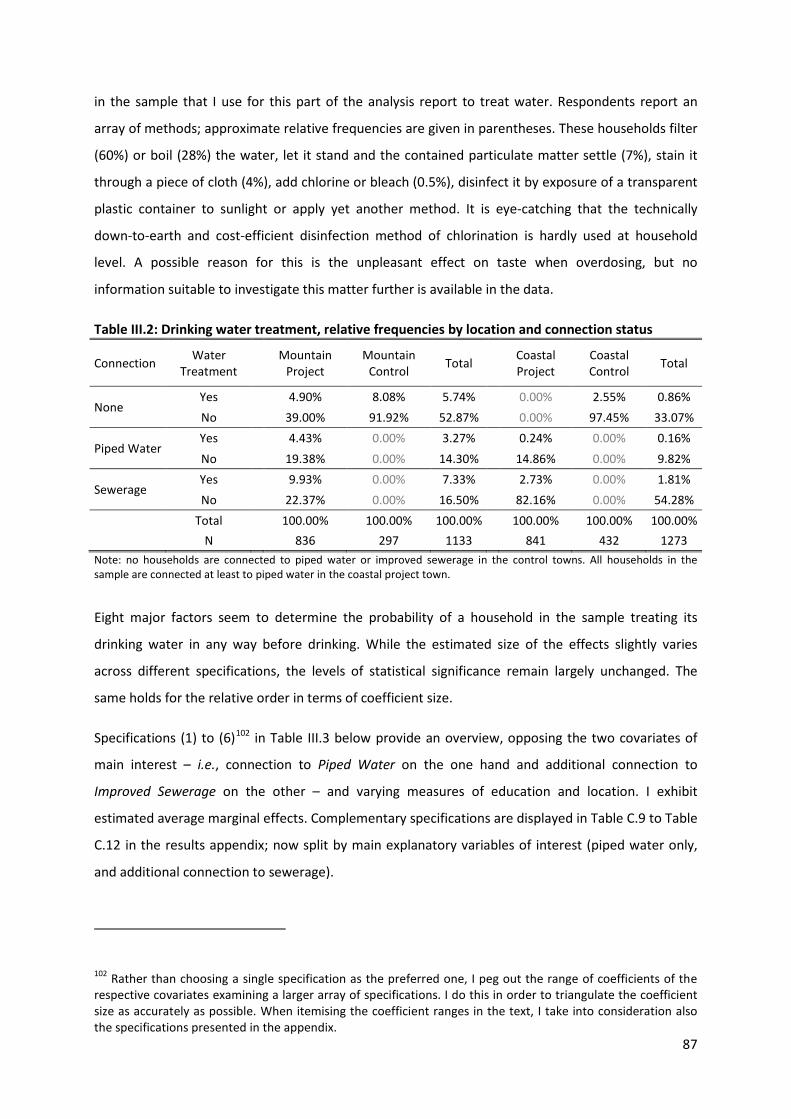
87

in the sample that I use for this part of the analysis report to treat water. Respondents report an

array of methods; approximate relative frequencies are given in parentheses. These households filter

(60%) or boil (28%) the water, let it stand and the contained particulate matter settle (7%), stain it

through a piece of cloth (4%), add chlorine or bleach (0.5%), disinfect it by exposure of a transparent

plastic container to sunlight or apply yet another method. It is eye-catching that the technically

down-to-earth and cost-efficient disinfection method of chlorination is hardly used at household

level. A possible reason for this is the unpleasant effect on taste when overdosing, but no

information suitable to investigate this matter further is available in the data.

Table III.2: Drinking water treatment, relative frequencies by location and connection status

Connection Water Treatment

Mountain Project

Mountain Control Total

Coastal Project

Coastal Control Total

None Yes 4.90% 8.08% 5.74% 0.00% 2.55% 0.86% No 39.00% 91.92% 52.87% 0.00% 97.45% 33.07%

Piped Water Yes 4.43% 0.00% 3.27% 0.24% 0.00% 0.16% No 19.38% 0.00% 14.30% 14.86% 0.00% 9.82%

Sewerage Yes 9.93% 0.00% 7.33% 2.73% 0.00% 1.81% No 22.37% 0.00% 16.50% 82.16% 0.00% 54.28%

Total 100.00% 100.00% 100.00% 100.00% 100.00% 100.00%

N 836 297 1133 841 432 1273 Note: no households are connected to piped water or improved sewerage in the control towns. All households in the sample are connected at least to piped water in the coastal project town.

Eight major factors seem to determine the probability of a household in the sample treating its

drinking water in any way before drinking. While the estimated size of the effects slightly varies

across different specifications, the levels of statistical significance remain largely unchanged. The

same holds for the relative order in terms of coefficient size.

Specifications (1) to (6)102 in Table III.3 below provide an overview, opposing the two covariates of

main interest – i.e., connection to Piped Water on the one hand and additional connection to

Improved Sewerage on the other – and varying measures of education and location. I exhibit

estimated average marginal effects. Complementary specifications are displayed in Table C.9 to Table

C.12 in the results appendix; now split by main explanatory variables of interest (piped water only,

and additional connection to sewerage).

102 Rather than choosing a single specification as the preferred one, I peg out the range of coefficients of the respective covariates examining a larger array of specifications. I do this in order to triangulate the coefficient size as accurately as possible. When itemising the coefficient ranges in the text, I take into consideration also the specifications presented in the appendix.

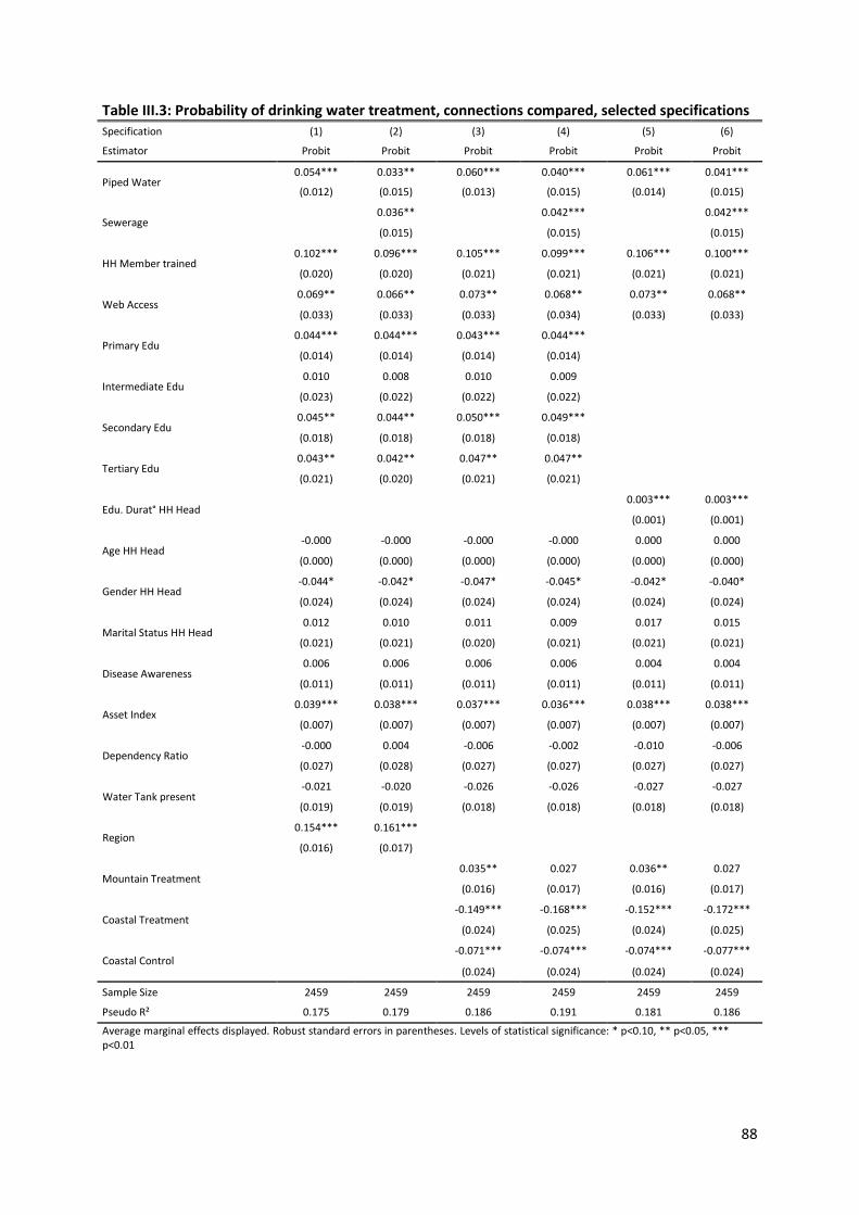
88

Table III.3: Probability of drinking water treatment, connections compared, selected specifications Specification (1) (2) (3) (4) (5) (6)

Estimator Probit Probit Probit Probit Probit Probit

Piped Water 0.054*** 0.033** 0.060*** 0.040*** 0.061*** 0.041***

(0.012) (0.015) (0.013) (0.015) (0.014) (0.015)

Sewerage 0.036** 0.042*** 0.042***

(0.015) (0.015) (0.015)

HH Member trained 0.102*** 0.096*** 0.105*** 0.099*** 0.106*** 0.100***

(0.020) (0.020) (0.021) (0.021) (0.021) (0.021)

Web Access 0.069** 0.066** 0.073** 0.068** 0.073** 0.068**

(0.033) (0.033) (0.033) (0.034) (0.033) (0.033)

Primary Edu 0.044*** 0.044*** 0.043*** 0.044*** (0.014) (0.014) (0.014) (0.014)

Intermediate Edu 0.010 0.008 0.010 0.009

(0.023) (0.022) (0.022) (0.022)

Secondary Edu 0.045** 0.044** 0.050*** 0.049*** (0.018) (0.018) (0.018) (0.018)

Tertiary Edu 0.043** 0.042** 0.047** 0.047** (0.021) (0.020) (0.021) (0.021)

Edu. Durat° HH Head 0.003*** 0.003***

(0.001) (0.001)

Age HH Head -0.000 -0.000 -0.000 -0.000 0.000 0.000

(0.000) (0.000) (0.000) (0.000) (0.000) (0.000)

Gender HH Head -0.044* -0.042* -0.047* -0.045* -0.042* -0.040*

(0.024) (0.024) (0.024) (0.024) (0.024) (0.024)

Marital Status HH Head 0.012 0.010 0.011 0.009 0.017 0.015

(0.021) (0.021) (0.020) (0.021) (0.021) (0.021)

Disease Awareness 0.006 0.006 0.006 0.006 0.004 0.004

(0.011) (0.011) (0.011) (0.011) (0.011) (0.011)

Asset Index 0.039*** 0.038*** 0.037*** 0.036*** 0.038*** 0.038***

(0.007) (0.007) (0.007) (0.007) (0.007) (0.007)

Dependency Ratio -0.000 0.004 -0.006 -0.002 -0.010 -0.006

(0.027) (0.028) (0.027) (0.027) (0.027) (0.027)

Water Tank present -0.021 -0.020 -0.026 -0.026 -0.027 -0.027

(0.019) (0.019) (0.018) (0.018) (0.018) (0.018)

Region 0.154*** 0.161*** (0.016) (0.017)

Mountain Treatment 0.035** 0.027 0.036** 0.027

(0.016) (0.017) (0.016) (0.017)

Coastal Treatment -0.149*** -0.168*** -0.152*** -0.172***

(0.024) (0.025) (0.024) (0.025)

Coastal Control -0.071*** -0.074*** -0.074*** -0.077***

(0.024) (0.024) (0.024) (0.024)

Sample Size 2459 2459 2459 2459 2459 2459

Pseudo R² 0.175 0.179 0.186 0.191 0.181 0.186

Average marginal effects displayed. Robust standard errors in parentheses. Levels of statistical significance: * p<0.10, ** p<0.05, *** p<0.01

89

For reasons of space limitation I respectively portion the tables into specifications varying ICT

exposure variables on the one hand, and introduce location variables as well as alternative

estimation methods on the other hand. The alternative estimators are intended to control for

endogeneity, and second stages are displayed. The results of these latter specifications (see Table

C.11 and Table C.12) as well as results of first stages (see Table C.29) are displayed in Appendix C.6.

The coefficients of determination of the models range from 17 to 19 per cent.

The most influential covariates in terms of coefficient size are those indicating the location of the

household. The household being located in the mountainous area103 appears to increase the

probability of treating its drinking water before consumption by 15 to 16 per cent, compared to

location in the coastal plain. Other explanatory variables with the same positive sign of coefficients –

always statistically significant at conventional levels, if not mentioned otherwise – include, roughly in

descending order of absolute coefficient size (in all specifications): previous participation of any

household member in a Hygiene Training (with an estimated effect size of about ten per cent),104 and

connection either to Piped Water only (5 to 6%) or additionally to Improved Sewerage (3 to 4%).

Exposure to information and communication technology constitutes itself in varying correlation

coefficient sizes, depending on which measure is included in the specification. I measure ICT

exposure using seven alternative variables.105

The most influential of these seems to be access to the World Wide Web. Correlation coefficients

indicate marginal effect sizes ranging from about three (radio receiver) to seven per cent (web

access). The level of Education of the household head appears to be an influential determinant as

well, with a non-linear course. Compared to the reference category “no education”, I estimate

completed primary education to increase the probability of treatment of drinking water by four to

five per cent. Intermediate education comes with no statistical significance at conventional levels,

while the effects of completed secondary and tertiary education each equal that of primary

education. I estimate wealth, proxied by the Asset Index, to have a marginal effect size of three to

four per cent. The Gender of the household head being male, in contrast, seems to decrease the

probability by four to five per cent.

103 Interestingly, when including the variable Sewerage on top of Piped Water, the coefficient of the categorical variable indicating location in the mountain treatment town (reference category is mountain control town) changes its level of statistical significance from the 95-percent level to below 90-percent level. 104 Marginal effects indicated in parentheses are approximate values. Numbers slightly vary over specifications, mostly only at the third decimal place. 105 These seven ICT variables are: presence of a Television Set, a Personal Computer, a Satellite Dish antenna (these three do not seem to play a role), a Radio Receiver, a Cell Phone; connection to a telephone Landline, and to the World Wide Web.

90

The estimated coefficients of some explanatory variables – ex ante conceived to have a measurable

effect – turn out to lack any statistical significance at conventional levels. Age and Marital Status of

the household head seem to have no influence on the probability of water treatment. The same is

true for the respondent knowing about causal relationships of any symptoms of water-related

diseases with water quality, sewerage and hygienic conditions (Disease Awareness). Likewise, the

illness history of household members reflected by Symptom Occurrence during the last month before

the interview does not appear to be a determinant. The same is true for the Dependency Ratio106 and

presence of a Water Storage Tank. Interacting Gender and Level of Education of the household head

did not yield any effect.

To test for robustness of results I use different specifications changing variables and estimation

procedures. I use varying measures of exposure to ICT, alternative location variables, household

composition and education measures, and wealth proxies. Furthermore, I exclude – one at a time –

selected variables (e.g. using either Disease Awareness or Symptom Occurrence). The estimations are

robust over all specifications for most107 of the explanatory variables regarding levels of statistical

significance, direction of sign and relative coefficient size. Within estimation procedures, also the

absolute coefficient sizes remain stable.

Besides 1) Probit regressions I also employ 2) 2SPrB (a two-stage Probit bootstrap, see Appendix C.4

for details on this and the following estimators), 3) RSUR BP (a recursive version of SUR BP), 4) IV-

Probit, and 5) W2SLS (a specific two-stage procedure proposed by Wooldridge 2010) to control for

endogeneity. All of these display levels of statistical significance and coefficient signs108 mostly

consistent with all of the basic Probit models for most of the explanatory and control variables. This

hints toward the absence of a noteworthy endogeneity bias, but it has to be kept in mind that due to

the doubts raised above regarding the fulfilment of the exogeneity condition, these findings are

circumstantial evidence at best.

It turns out that some, but not all of the hypotheses can be corroborated. Strong evidence is found

that Hypothesis 3a (those households in which at least one member participated in any type of

106 The Dependency Ratio is statistically significant mainly in specifications without location variables. 107 There are two exceptions. The level of statistical significance of the variable Gender of Household Head drops below the ten per cent convention in a few of the specifications. Presence of a Water Storage Tank features coefficients statistically significant at conventional levels only when using the IV-Probit or W2SLS estimator, in each of the cases with a negative sign. 108 Relative coefficient sizes within the IV models do not always reflect those of the Probit model. Some variables seem to gain prediction power on cost of others. The most important covariates in terms of effect size keep their position, though. Absolute coefficient sizes may differ from the marginal effects estimated with the Probit model.

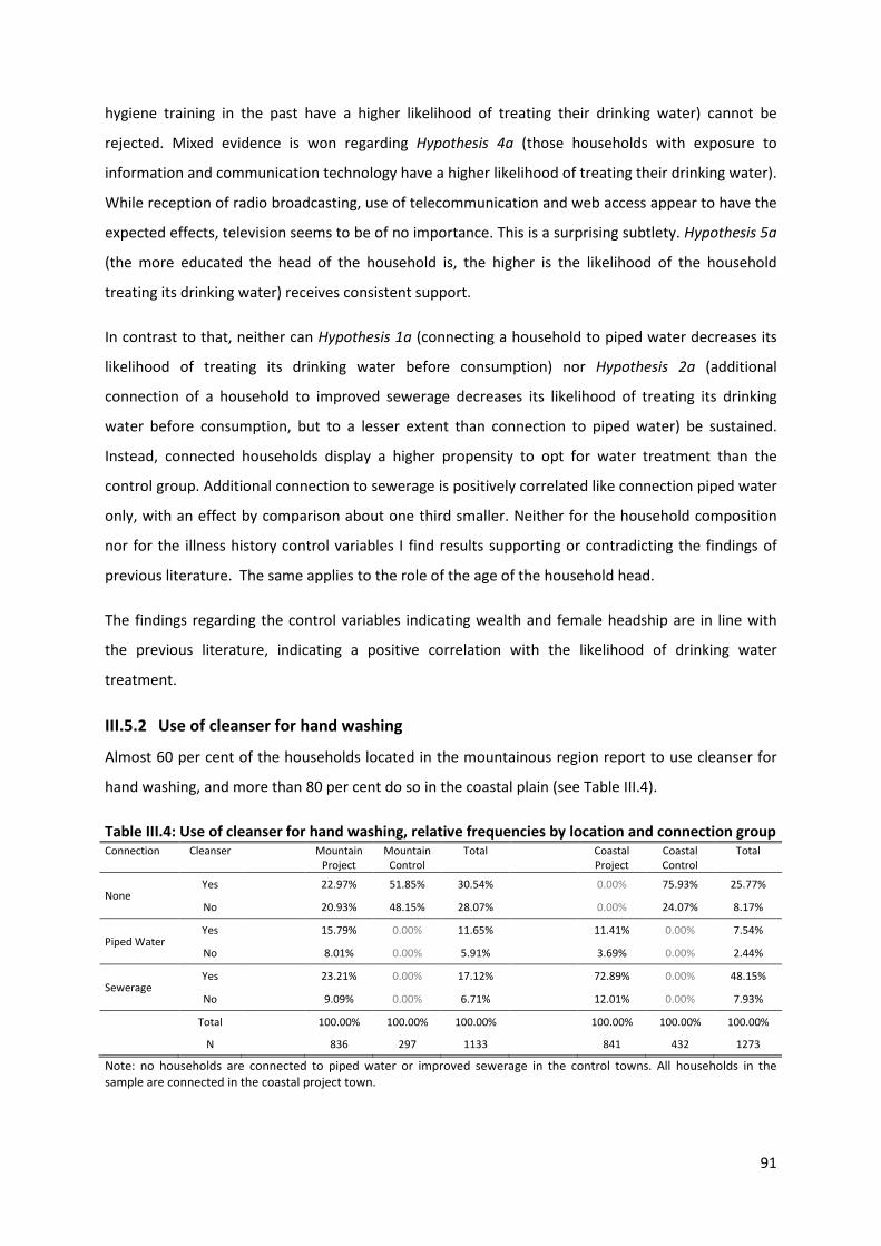
91

hygiene training in the past have a higher likelihood of treating their drinking water) cannot be

rejected. Mixed evidence is won regarding Hypothesis 4a (those households with exposure to

information and communication technology have a higher likelihood of treating their drinking water).

While reception of radio broadcasting, use of telecommunication and web access appear to have the

expected effects, television seems to be of no importance. This is a surprising subtlety. Hypothesis 5a

(the more educated the head of the household is, the higher is the likelihood of the household

treating its drinking water) receives consistent support.

In contrast to that, neither can Hypothesis 1a (connecting a household to piped water decreases its

likelihood of treating its drinking water before consumption) nor Hypothesis 2a (additional

connection of a household to improved sewerage decreases its likelihood of treating its drinking

water before consumption, but to a lesser extent than connection to piped water) be sustained.

Instead, connected households display a higher propensity to opt for water treatment than the

control group. Additional connection to sewerage is positively correlated like connection piped water

only, with an effect by comparison about one third smaller. Neither for the household composition

nor for the illness history control variables I find results supporting or contradicting the findings of

previous literature. The same applies to the role of the age of the household head.

The findings regarding the control variables indicating wealth and female headship are in line with

the previous literature, indicating a positive correlation with the likelihood of drinking water

treatment.

III.5.2 Use of cleanser for hand washing

Almost 60 per cent of the households located in the mountainous region report to use cleanser for

hand washing, and more than 80 per cent do so in the coastal plain (see Table III.4).

Table III.4: Use of cleanser for hand washing, relative frequencies by location and connection group Connection Cleanser Mountain

Project Mountain

Control Total Coastal

Project Coastal Control

Total

None Yes 22.97% 51.85% 30.54% 0.00% 75.93% 25.77%

No 20.93% 48.15% 28.07% 0.00% 24.07% 8.17%

Piped Water Yes 15.79% 0.00% 11.65% 11.41% 0.00% 7.54%

No 8.01% 0.00% 5.91% 3.69% 0.00% 2.44%

Sewerage Yes 23.21% 0.00% 17.12% 72.89% 0.00% 48.15%

No 9.09% 0.00% 6.71% 12.01% 0.00% 7.93%

Total 100.00% 100.00% 100.00% 100.00% 100.00% 100.00%

N 836 297 1133 841 432 1273

Note: no households are connected to piped water or improved sewerage in the control towns. All households in the sample are connected in the coastal project town.

92

The percentage of compliers (i.e., households that use cleanser) is larger than that of non-compliers

in all four towns and three connection status groups (not connected, piped water only, combination

of piped water with improved sewerage). It has to be noted that this might partly reflect a positive

reporting bias as discussed in the data section. This potential bias is assumed to be non-systematic,

i.e. not dependent on town or connection status.

Ten major factors seem to determine the probability of a household head in the sample using

cleanser when washing hands. I identify nine explanatory variables or groups of variables which are

positively correlated with the probability of using cleanser; and one which is negatively correlated.

Keeping the structure of covariates consistent with the overview table presented for the former

dependent variable, I oppose the two covariates of main interest in specifications (1) to (6) in Table

III.5 below. Estimated marginal effects are indicated in parentheses as approximate percentage

change of probability of use of cleanser.

Table C.13 to Table C.16 in Appendix C.6 display the estimated marginal effects for complementary

specifications. As above, the tables are split by main explanatory variables of interest; and

specifications vary media exposure, location, education and household composition variables. Again,

for reasons of space limitation alternative specifications and estimators (see Table C.15 and Table

C.16) as well as results of first stages (see Table C.29) are presented in the same appendix. The

coefficient of determination of the models ranges from eight to eleven per cent.

The mentioned variables comprise, approximately in descending order of absolute coefficient size:

location in the Coastal Control (20 to 21 per cent over reference location Mountain Control) or

Project (18 to 19%) Town, connection to the Piped Water network (10 to 12%), the Level of Education

of the household head (in contrast to before though no longer for Primary Education, with eight to

nine per cent for Secondary Education over reference category “No Education”, and Tertiary with

nine to ten per cent), participation of a household member in a Hygiene Training (9 to 10 %),

Exposure to ICT109 (4 to 9%), additional connection to the Improved Sewerage network (5%,

statistically less significant than Piped Water), Disease Awareness (4%), Symptom Occurrence (3%)

and Assets as a proxy for wealth (3 to 4%).

109 In contrast to before, presence of a television set is now statistically significant at the ten per cent level, presence of a satellite dish even at the one per cent level. Interestingly, web access is no longer significant at conventional levels. I observe the strongest effect for landline phone connection.

93

Table III.5: Probability of cleanser use, connections compared, selected specifications Specification (1) (2) (3) (4) (5) (6)

Estimator Probit Probit Probit Probit Probit Probit

Piped Water 0.100*** 0.078*** 0.124*** 0.101*** 0.118*** 0.096***

(0.018) (0.024) (0.024) (0.027) (0.024) (0.027)

Sewerage 0.037 0.049* 0.048*

(0.027) (0.027) (0.027)

HH Member trained 0.092* 0.087* 0.093* 0.087* 0.090* 0.084*

(0.050) (0.050) (0.050) (0.050) (0.049) (0.049)

Web Access 0.031 0.028 0.032 0.029 0.027 0.023

(0.084) (0.084) (0.083) (0.083) (0.083) (0.083)

Primary Edu -0.006 -0.007 -0.005 -0.006 (0.024) (0.024) (0.024) (0.024)

Intermediate Edu 0.051 0.048 0.054 0.052

(0.039) (0.039) (0.039) (0.039)

Secondary Edu 0.081*** 0.078*** 0.084*** 0.082*** (0.028) (0.028) (0.028) (0.028)

Tertiary Edu 0.095*** 0.093*** 0.099*** 0.097*** (0.032) (0.032) (0.031) (0.031)

Edu. Durat° HH Head 0.009*** 0.009***

(0.002) (0.002)

Age HH Head 0.000 0.000 0.000 0.000 0.001 0.001

(0.001) (0.001) (0.001) (0.001) (0.001) (0.001)

Gender HH Head 0.002 0.004 -0.001 0.001 -0.016 -0.014

(0.046) (0.046) (0.046) (0.046) (0.046) (0.046)

Marital Status HH Head

-0.001 -0.002 0.000 -0.002 -0.001 -0.003

(0.040) (0.040) (0.040) (0.040) (0.040) (0.040)

Disease Awareness 0.042** 0.042** 0.042** 0.042** 0.039** 0.039**

(0.018) (0.018) (0.017) (0.017) (0.017) (0.017)

Asset Index 0.044*** 0.043*** 0.043*** 0.042*** 0.041*** 0.040***

(0.013) (0.013) (0.013) (0.013) (0.013) (0.013)

Dependency Ratio -0.193*** -0.188*** -0.197*** -0.191*** -0.204*** -0.198***

(0.041) (0.041) (0.041) (0.041) (0.041) (0.041)

Water Tank present 0.017 0.016 0.012 0.009 0.009 0.007

(0.024) (0.024) (0.024) (0.024) (0.024) (0.024)

Region -0.183*** -0.177***

(0.020) (0.020)

Mountain Treatment 0.003 -0.004 0.004 -0.003

(0.027) (0.027) (0.027) (0.027)

Coastal Treatment 0.154*** 0.134*** 0.152*** 0.132***

(0.035) (0.037) (0.035) (0.037)

Coastal Control 0.214*** 0.210*** 0.214*** 0.210***

(0.031) (0.031) (0.031) (0.031)

Sample Size 2466 2466 2466 2466 2466 2466

Pseudo R² 0.088 0.088 0.089 0.090 0.092 0.093

Average marginal effects displayed. Robust standard errors in parentheses. Levels of statistical significance: * p<0.10, ** p<0.05, *** p<0.01

94

Opposing these nine factors is one which is negatively correlated with the probability of using

cleaner. An increase of the Dependency Ratio by one appears to reduce the probability by up to one

fifth (-15 to -20%).

It comes somewhat unexpected that certain factors do not seem to have any influence. These

include the presence of a Water Storage Tank, or Primary Education of the household head –

remember I above show both of the latter to be correlated with treatment of drinking water. The

same is true for personal characteristics of the household head as Age, and Marital Status.

It is noteworthy that in contrast to my former dependent variable – probability of treatment of

drinking water before consumption – the probability of cleanser use does not appear to be

correlated with the Gender of the household head.

I check for robustness of the results by estimating different specifications. The estimations are robust

over all specifications for almost all of the explanatory variables regarding levels of statistical

significance, direction of sign and relative coefficient size. In addition, over different specifications,

the absolute coefficient sizes remain stable. Apart from two instrumental variable specifications, in

which the location variable coefficient switches sign,110 there is only one group of variables that

requires a closer look. Varying measures of exposure to ICT sheds light on heterogeneous intensities

of correlation with cleanser use. While the coefficients of presence of a Landline, Cell phone, a

Satellite Dish or Radio Receiver come with statistical significance at the five per cent level or higher,

access to the World Wide Web does not seem to play any role. Possession of a Television Set of a

household is correlated with the probability of use of cleanser stronger and at a higher level of

statistical significance when the household has more members111 than others. One possible

explanation is that this finding might reflect the effect of a larger audience (i.e., the television set

might be powered during more time of the day, and the household head pick up more information).

When the household is connected to Improved Sewerage presence of a Satellite Dish is significant at

the one per cent level, and thus at a higher level than those connected to piped water only (5%).

As before, all of the estimators employed112 to control for endogeneity display levels of statistical

significance and coefficient signs mostly consistent with all of the basic Probit models for most of the

110 Refer to Kennedy (2005) for a thorough discussion of possible causes of “wrong” signs of estimated coefficients. As the switching of sign occurs only twice, I regard the matter not to be overly concerning. 111 This is respectively reflected by the following household composition variables: number of children, number of children and elderly, and total number of household members. 112 The same four instrumental variable estimators are used as for the dependent variable Probability of drinking water treatment: 2SPrB, RSUR BP, IV-Probit, and W2SLS.

95

explanatory and control variables. As mentioned before in context with the first dependent variable,

the Sargan-Hansen test indicates that the instruments do not fulfil the exogeneity condition.

Therefore the results of these estimators are of limited informative value.

Deliberating the findings on the probability of cleanser use as a dependent variable, I come to the

conclusion that none of my hypotheses – here listed in order of estimated effect sizes of their

respective variables – can be rejected. Hypothesis 1b (connecting a household to piped

water increases its likelihood of displaying hygiene habits) appears to be correct. So does Hypothesis

5b (the more educated the head of the household is the higher is the likelihood of the household

members displaying hygiene habits), for secondary and tertiary education. Also Hypothesis 2b

(additional connection of a household to improved sewerage decreases its likelihood of displaying

hygiene habits, but to a lesser extent than connection to piped water) seems to reflect reality,

including its comparative second component. The same is true for Hypothesis 3b (those households

in which at least one member participated in any type of hygiene training in the past have a higher

likelihood of displaying hygiene habits). So does Hypothesis 4b (those households with exposure to

information and communication technology have a higher likelihood of displaying hygiene habits),

while web access and the variable TV and/or PC present constitute the exceptions: they are never

statistically significant. Regarding control variables, the picture is mixed. The coefficient of wealth

and disease awareness have the expected sign, while larger households in contrast to my expectation

seem to have a lower probability to use cleanser than smaller ones. Neither recent symptom

occurrence, nor age or gender of the household head seems to play a role.

As an additional approach to establish robustness of the findings; and to increase confidence that the

probability of cleanser use is indeed a good proxy for hygiene habits, I regress three alternative

continuous dependent variables on the covariates: Spending on Soap, Spending on Cleanser, and

Frequency of Latrine-cleaning. The findings are largely113 consistent with those of the present section.

I describe this in detail in Appendix C.6. The mentionable exceptions are that Improved Sewerage is

not statistically significant for the dependent variable Spending on Soap; and both connection types

are not statistically significant for the dependent variable Spending on Cleanser. In contrast to Piped

Water, Improved Sewerage is not statistically significant for the dependent Variable Latrine Cleaning

Frequency. The variable Hygiene Training is not statistically significant at conventional levels for the

dependent variable Spending on Soap, but for all four other dependent variables, including Spending

on Cleanser.

113 The variable hygiene training is not statistically significant at conventional levels for the dependent variable spending on soap, but for all four other dependent variables, including spending on cleanser.

96

III.6 Conclusion

The purpose of this chapter is to identify the determinants of water treatment and hygiene habits in

households in Yemenite provincial towns. I do this by empirically analysing micro-level data collected

during a large-scale household survey; and summarize the main findings as follows.

The probability of Drinking Water Treatment is positively correlated with location of the household in

the mountainous region, hygiene training experience, connection to piped water, additional

connection to improved sewerage, ICT exposure, and wealth, completed primary, secondary and

tertiary education. The gender of the household head being male, and the household being located

in the coastal plain – especially in the project town, is negatively correlated.

I use four different measures to map Hygiene Habits, i.e. the reported practices and resource

allocation on household level linked to personal hygiene and health-relevant aspects of

housekeeping. The measures are not chosen as stand-alone signifiers of hygiene habits, but are

intended to allow composing a more comprehensive and detailed picture of determinants of habitual

hygiene behaviour. The analysis reveals that connection to piped water is a more important driver

than that to improved sewerage. Participation in hygiene training is among the most strongly

correlated covariates. Wealth and recent affection foster hygiene habits. The same I can say about

ICT, while I have to challenge the idea that the underlying mechanism is entirely rooted in better

access to information. In the following, the four outcome variables are crisply covered one by one.

First, the probability of Use of Cleanser for hand washing appears to be fostered by location in the

coastal region, connection to piped water, level of education, hygiene training experience,

connection to improved sewerage, ICT exposure, disease awareness, recent illness history and

wealth. The dependency ratio is negatively correlated. Second, Spending on Soap is positively

correlated with ICT exposure, location in the mountainous region, and connection to piped water,

use of a water storage tank, wealth and recent illness history. Location in one of the coastal towns

and age of the household head are negatively correlated with spending. Third, Spending on Cleanser

(including laundry detergent) seems to be increased by ICT exposure, hygiene training experience,

location in the mountainous region, disease awareness, recent illness history, connection to piped

water (only in few of the specifications) and wealth. The dependency ratio, location in one of the

coastal towns and age of the household head are negatively correlated. Fourth, the Frequency of

Latrine-Cleaning appears to be driven by mean education duration of adults, training, the

dependency ratio, connection to piped water, wealth, location in the coastal project town, presence

of a water storage tank, and education. On the other hand, location in the coastal control town or in

the mountainous region is negatively correlated with the frequency.

97

It requires some thought how the findings of the chapter at hand can be squared with those of the

preceding one; and consecutive work by Lechtenfeld (2012). Chapter II carves out that piped water

deteriorates health (in the mountainous area) or has so significant effect (in the coastal area); and

improved sewerage has no significant (mountainous) to marginally improving (coastal) health effects.

We find that incidence of e.coli is high in treatment households, with more than half of it stemming

from leaking pipes and rationing; and the remainder from household behaviour. The findings of

Lechtenfeld (2012) are in line with this, stating that access to piped water increases the “risk of child

diarrhea by 4.6 percentage points”; with the majority of the pollution stemming from “broken pipes

and interruptions of water supply”, exacerbated by “unhygienic water storage and handling at

household level”. In Chapter III I now find that connection to piped water and also to improved

sewerage are positively correlated with the probability of drinking water treatment and reporting of

following hygiene habits. While this seems to contradict the detrimental to at best feeble health

impact of connection to piped water found in Chapter II and by Lechtenfeld (2012), three reconciling

explanations are conceivable: First, although connected households seem to display a higher

probability of treating their drinking water and of displaying hygiene habits, the beneficial effect of

this behaviour on health might be overcompensated by the detrimental effect of the connection on

health. Second, water treatment at the household level might – although implemented – be

ineffective for some reason, possibly faulty practices. It seems less likely to me that poor conduct of

hygiene practices might be an issue here, as water treatment is more technical and complicated than

body and living quarters hygiene. Third, the behaviour might be an adjustment reaction of connected

households realizing that the connection might increase the risk of contamination of the drinking

water at point-of-use. All three explanations underline that pollution caused on the supply side is a

major concern.

The study at hand faces two noteworthy limitations. First, all data used in the analysis is self-reported

information about behavioural aspects regarding various aspects of hygiene. Yemenite female

enumerators talking face to face for protracted time to women in the survey households conducted

the interviews. The potential concern that reporting could be biased in favour of behaviour deemed

by the respondents to meet the expectations of the enumerator cannot entirely be dismissed.

Craving for admiration might palliate the picture. Anyway, a good case can be made why not to have

to worry too much about this potential bias: there is no reason to believe that it should be systematic

in any way, i.e. affecting households in different ways depending on their location, social strata et

cetera. Neither did the interviewers report any peculiarities in this regard, nor did searching for

patterns in the data reveal anything hinting towards such systematic differences. Second, limited

98

subsample sizes restrict the explanatory power of the study regarding resource allocation. For

instance, data on expenditure on cleanser is available for no more than 118 households114 when

analysing those located in the coastal plain and connected to piped water, but not improved

sewerage. Nothing can be done to remedy this difficulty.

As presented in the introduction, Yemen is similar to many MENA countries – and beyond – in terms

of topography, hydrography, demography, public health and socio-economic development faced.

Admittedly, some of these circumstances are posing challenges of a more complex and urgent nature

in Yemen than elsewhere. However, conceptually comparable to the effect of a magnifying glass, due

to these intensifying circumstances – increasing the visibility of need for action – the country might

so much the better serve as a case study from which lessons can be learned for other countries and

societies. Mechanisms at work are presumed to become evident more articulate in the tightened

Yemenite setting. External validity can be insinuated inasmuch as those determinants identified in

this study to drive behaviour will probably be at work in other locations as well, albeit in varying

magnitudes of effect.

Several policy implications suggest themselves. I identify a couple of determinants of hygiene-related

behaviour that planners and designers of infrastructure projects in the water and sanitation section

can take into account. Furthermore, some of these determinants can be influenced in the medium

term in order to achieve more favourable health outcomes of such projects than up to now.

Especially flanking and complementing construction of piped water and sewerage from the outset

with hygiene training offers and health awareness campaigns networks – either based on multipliers

or with blanket coverage – shows promise.

Future research should address two main fields of interest. First, to my knowledge, nobody

conducted Randomized Controlled Trial (RCT) or quasi-experimental studies yet in order to establish

the optimal level of intensity, resource allocation and mode of conduct regarding hygiene trainings

and health awareness campaigns. This knowledge gap should be filled in order to improve integrated

development programme planning and cost-benefit ratios. Second, the role of ICT in shaping and

influencing perceptions, beliefs and habits regarding water handling practices and personal hygiene

should be inspected more closely. In particular, the shifting relevance of different media and devices

deserves attention. Gaugeable data and information should be attained on the role of the World

114 This is the lowest subsample size in this study. Data from the section of the questionnaire used to survey data on consumption expenditure is less exhaustive than that from other sections. Part of this is rooted in a certain reluctance demonstrated by many Yemenite households to disclose this particular kind of information.

99

Wide Web, social media and modern mobile telecommunication devices. Apart from that, the

questions analysed in the study at hand should be researched in other geographic regions, with

samples of sufficient size to ensure validity of findings for all sub-groups of the surveyed population.

100

101

Bibliography

Adelman, Madelaine (2003): The military, militarism, and the militarization of domestic violence. In

Violence Against Women 9 (9), pp. 1118–1152.

Adkins, Lee C. (2009): An Instrumental Variables Probit Estimator using gretl. In Ignacio Diaz-

Emparanza, Petr Mariel, Maria Victoria Esteban (Eds.): Econometrics with gretl. Proceedings

of the gretl conference 2009. Bilbao.

Ai, Chunrong; Norton, Edward C. (2003): Interaction terms in logit and probit models. In Economics

Letters 80 (1), pp. 123–129.

Aiello, Allison E.; Coulborn, Rebecca M.; Perez, Vanessa; Larson, Elaine L. (2008): Effect of hand

hygiene on infectious disease risk in the community setting: a meta-analysis. In American

Journal of Public Health 98 (8), pp. 1372–1381.

Aizer, Anna (2010): The gender wage gap and domestic violence. In American Economic Review 100

(4), pp. 1847–1859.

Angrist, Joshua D. (2001): Estimation of limited dependent variable models with dummy endogenous

regressors. In Journal of Business & Economic Statistics 19 (1), pp. 2–16.

Angrist, Joshua D.; Pischke, Jörn-Steffen (2008): Mostly harmless econometrics: An empiricist's

companion. Princeton, NJ: Princeton University Press.

Angrist, Joshua; Krueger, Alan B. (2001): Instrumental variables and the search for identification:

From supply and demand to natural experiments. In Journal of Economic Perspectives 15 (4),

pp. 69–85.

Aunger, Robert; Schmidt, Wolf-Peter; Ranpura, Ashish; Coombes, Yolande; Maina, Peninnah Mukiri;

Matiko, Carol Nkatha; Curtis, Valerie (2010): Three kinds of psychological determinants for

hand-washing behaviour in Kenya. In Social Science and Medicine 70 (3), pp. 383–391.

Badowski, Natalie; Castro, Cynthia M.; Montgomery, Maggie; Pickering, Amy J.; Mamuya, Simon;

Davis, Jennifer (2011): Understanding household behavioral risk factors for diarrheal disease

in Dar es Salaam: A photovoice community assessment. In Journal of Environmental and

Public Health 2011.

Barry, Michele; Hughes, James M. (2008): Talking dirty – the politics of clean water and sanitation. In

New England Journal of Medicine 359 (8), pp. 784–787.

Bartram, Jamie; Lewis, Kristen; Lenton, Roberto; Wright, Albert (2005): Focusing on improved water

and sanitation for health. In The Lancet 365 (9461), pp. 810–812.

102

Begum, Sharifa; Ahmed, Mansur; Sen, Binayak (2011): Do Water and Sanitation Interventions Reduce

Childhood Diarrhoea? New Evidence from Bangladesh. In Bangladesh Development Studies

34 (3), pp. 1–30.

Berkman, Douglas S.; Lescano, Andres G.; Gilman, Robert H.; Lopez, Sonia L.; Black, Maureen M.

(2002): Effects of stunting, diarrhoeal disease, and parasitic infection during infancy on

cognition in late childhood: a follow-up study. In The Lancet 359 (9306), pp. 564–571.

Bernheim, B. Douglas; Garrett, Daniel M.; Maki, Dean M. (2001): Education and saving:: The long-

term effects of high school financial curriculum mandates. In Journal of Public Economics 80

(3), pp. 435–465.

Black, Robert E.; Morris, Saul S.; Bryce, Jennifer (2003): Where and why are 10 million children dying

every year? In The Lancet 361 (9376), pp. 2226–2234.

Blattman, Christopher (2009): From Violence to Voting: War and political participation in Uganda. In

American Political Science Review 103 (2), pp. 231–247.

Blattman, Christopher; Miguel, Edward (2010): Civil war. In Journal of Economic Literature 48 (1), pp.

3–57.

Brett, Eduard A. (2003): Participation and accountability in development management. In Journal of

Development Studies 40 (2), pp. 1–29.

Brikké, François; Bredero, Maarten (2003): Linking technology choice with operation and

maintenance in the context of community water supply and sanitation. Reference document

for planners and project staff. World Health Organization and IRC International Water and

Sanitation Centre. Geneva.

Burton, Maxine; Cobb, Emma; Donachie, Peter; Judah, Gaby; Curtis, Val; Schmidt, Wolf-Peter (2011):

The effect of handwashing with water or soap on bacterial contamination of hands. In

International Journal of Environmental Research and Public Health 8 (1), pp. 97–104.

Cairncross, Sandy; Hunt, Caroline; Boisson, Sophie; Bostoen, Kristof; Curtis, Val; Fung, Isaac C. H.;

Schmidt, Wolf-Peter (2010): Water, sanitation and hygiene for the prevention of diarrhoea.

In International Journal of Epidemiology 39 (1), pp. 193–205.

Calderón, Valentina; Gáfaro, Margarita; Ibáñez, Ana María (2011): Forced Migration, Female Labor

Force Participation, and Intra-household Bargaining: Does Conflict Empower Women.

MICROCON (Research Working Paper, 56).

103

Carrasco, Raquel (2001): Binary choice with binary endogenous regressors in panel data: Estimating

the effect of fertility on female labor participation. In Journal of Business and Economic

Statistics 19 (4), pp. 385–394.

Central Intelligence Agency (2013): World Factbook. Central Intelligence Agency. Langley, VA.

Available online at https://www.cia.gov/library/publications/the-world-factbook/, last

accessed July 30, 2013.

Chase, Claire; Do, Quy Toan (2012): Handwashing behavior change at scale: evidence from a

randomized evaluation in Vietnam. World Bank (Policy Research Working Paper, 6207).

Chiburis Das Lokshin (2011): A Practical Comparison of the Bivariate Probit and Linear IV Estimators.

World Bank (Policy Research Working Paper, 5601).

Clasen, Thomas; Schmidt, Wolf-Peter; Rabie, Tamer; Roberts, Ian; Cairncross, Sandy (2007):

Interventions to improve water quality for preventing diarrhoea: systematic review and

meta-analysis. In British Medical Journal 334 (7597), p. 782.

Colorado Department of Human Services (2010): Domestic Violence Program. 2010 Annual Report.

Denver, CO.

Curtis, Val; Cairncross, Sandy (2003): Effect of washing hands with soap on diarrhoea risk in the

community: a systematic review. In The Lancet Infectious Diseases 3 (5), pp. 275–281.

Curtis, Val; Schmidt, Wolf; Luby, Stephen; Florez, Rocio; Touré, Ousmane; Biran, Adam (2011):

Hygiene: new hopes, new horizons. In The Lancet Infectious Diseases 11 (4), pp. 312–321.

Davis, Jennifer; Pickering, Amy J.; Rogers, Kirsten; Mamuya, Simon; Boehm, Alexandria B. (2011): The

effects of informational interventions on household water management, hygiene behaviors,

stored drinking water quality, and hand contamination in peri-urban Tanzania. In American

Journal of Tropical Medicine and Hygiene 84 (2), p. 184.

Devine, Jacqueline (2010): Beyond tippy-taps: The role of enabling products in scaling up and

sustaining handwashing. In Waterlines 29 (4), pp. 304–314.

DIVA-GIS (2013) Spatial Data. Available at: http://www.diva-gis.org/Data, last accessed June 13,

2013.

Dong, Yingying; Lewbel, Arthur (2012): A simple estimator for binary choice models with endogenous

regressors. Boston College (Boston College Working Papers in Economics, 807). Available

online at fmwww.bc.edu/EC-P/wp807.pdf.

104

Dreher, Axel; Klasen, Stephan; Raymond, James; Werker, Eric (2010): The costs of favoritism: Is

politically-driven aid less effective? Center for European, Governance and Economic

Development Research, University of Göttingen (CeGE Discussion Papers, 97).

Dupas, Pascaline (2011): Health behavior in developing countries. In Annual Review of Economics 3

(1), pp. 425–449.

Durevall, Dick; Lindskog, Annika (2013): Intimate Partner Violence and HIV in Sub-Saharan Africa.

Department of Economics, University of Gothenburg (Working Papers in Economics, 563).

Ebrahim, Alnoor (2003): Accountability in practice: mechanisms for NGOs. In World Development 31

(5), pp. 813–829.

Ejemot-Nwadiaro, Regina I.; Ehiri, John E.; Meremikwu, Martin M.; Critchley, Julia A. (2012): Hand

washing for preventing diarrhoea (Review). In The Cochrane Library (2), pp. 1–39.

Elbers, Chris; Godfrey, Samuel; Gunning, Jan; van der Velden, Matteus; Vigh, Melinda (2012):

Effectiveness of Large Scale Water and Sanitation Interventions: The One Million Initiative in

Mozambique. Tinbergen Institute. Amsterdam (Tinbergen Institute Discussion Papers, 12-

069/2).

Esrey, Steve A.; Potash, James B.; Roberts, Leslie; Shiff, Clive (1991): Effects of improved water supply

and sanitation on ascariasis, diarrhoea, dracunculiasis, hookworm infection, schistosomiasis,

and trachoma. In Bulletin of the World Health Organization 69 (5), p. 609.

Fan, Victoria Yue-May; Mahal, Ajay (2011): What prevents child diarrhoea? The impacts of water

supply, toilets, and hand-washing in rural India. In Journal of Development Effectiveness 3

(3), pp. 340–370.

Farmer, Amy; Tiefenthaler, Jill (1997): An economic analysis of domestic violence. In Review of Social

Economy 55 (3), pp. 337–358.

Feil, E. J. (2012): The emergence and spread of dysentery. In Nature Genetics 44 (9), pp. 964–965.

Fewtrell, Lorna; Kaufmann, Rachel B.; Kay, David; Enanoria, Wayne; Haller, Laurence; Colford Jr, John

M.(2005): Water, sanitation, and hygiene interventions to reduce diarrhoea in less developed

countries: a systematic review and meta-analysis. In The Lancet Infectious Diseases 5 (1), pp.

42–52.

Fink, Günther; Günther, Isabel; Hill, Kenneth (2011): The effect of water and sanitation on child

health: evidence from the demographic and health surveys 1986–2007. In International

Journal of Epidemiology 40 (5), pp. 1196–1204.

105

Fishman, Raymond; Miguel, Edward (2008): Economic Gangsters: Princeton University Press.

Flemming, Hans-Curt (2009): Marine and Industrial Biofouling. Why Microorganisms live in biofilms

and the problem of biofouling. In Springer Series on Biofilms (4), pp. 3–12.

Food and Agriculture Organization of the United Nations (2000) ‘Global Forest Resources Assessment

2000 (FRA 2000)’, available at: http://www.fao.org/forestry/32203/en/, last accessed June

13, 2013.

Fonagy, Peter (1999): Male perpetrators of violence against women: An attachment theory

perspective. In Journal of Applied Psychoanalytic Studies 1 (1), pp. 7–27.

Freedman, David A.; Sekhon, Jasjeet S. (2010): Endogeneity in probit response models. In Political

Analysis 18 (2), pp. 138–150.

Galiani, Sebastian; Gertler, Paul; Orsola-Vidal, Alexandra (2012): Promoting handwashing behavior in

Peru: the effect of large-scale mass-media and community level interventions. Impact

Evaluation Series No. 74. World Bank (Policy Research Working Paper, 6257).

Galiani, Sebastian; Gertler, Paul; Schargrodsky, Ernesto (2005): Water for life: The impact of the

privatization of water services on child mortality. In Journal of Political Economy 113 (1), pp.

83–120.

Gallegos, José; Gutierrez, Italo (2011): The Effect of Civil Conflict on Domestic Violence: the Case of

Peru (SSRN Working Paper Series). Available online at http://dx.doi.org/10.2139/ssrn.190441

7, last accessed July 30, 2013.

Gamper-Rabindran, Shanti; Khan, Shakeeb; Timmins, Christopher (2010): The impact of piped water

provision on infant mortality in Brazil: A quantile panel data approach. In Journal of

Development Economics 92 (2), pp. 188–200.

Garcés, Laura (2005): Colombia: the link between drugs and terror. In Journal of Drug Issues 35 (1),

pp. 83–105.

García-Moreno, Claudia; Jansen, HAFM; Ellsberg, Mary; Heise, Lori; Watts, Charlotte (2005): WHO

multi-country study on women's health and domestic violence against women. Geneva:

World Health Organization.

Greene, William H. (2012): Econometric Analysis. 7th ed. Upper Saddle River, NJ: Prentice hall.

Gundry, Stephen; Conroy, Ronan; Wright, Jim (2003): A systematic review of the health outcomes

related to household water quality in developing countries. In Journal of Water and Health 2

(1), pp. 1–13.

106

Haidera, Mansour; Alhakimi, Saif Ali; Noaman, Abdulla; Al Kebsi, Alkhatib; Noaman, Anwar; Fencl,

Amanda; Dougherty, Bill; Swartz, Chris (2011): Water scarcity and climate change adaptation

for Yemen's vulnerable communities. In Local Environment 16 (5), pp. 473–488.

Hardin, James W. (2012): Bivariate probit models. In Stata Technical Bulletin 6 (33), pp. 15–20.

Heckman, James J. (1978): Dummy endogenous variables in a simultaneous equation system. In

Econometrica 46 (4), pp. 931–959.

Heckman, James J. (1979): Sample selection bias as a specification error. In Econometrica 47 (1), pp.

153–161.

Hidrobo, M.; Fernald, L. (2013): Cash transfers and domestic violence. In Journal of Health Economics

32 (1), pp. 304–319.

Holm, Anders; Arendt, Jacob N. (2012): Evaluating the performance of simple estimators for

probit models with two dummy endogenous regressors. In Journal of Statistical Computation

and Simulation (ahead-of-print), pp. 1–23.

International Center for Tropical Agriculture (CIAT) 90m SRTM Data. Available at:

http://srtm.csi.cgiar.org/, last accessed June 13, 2013.

Jalan, Jyotsna; Ravallion, Martin (2003): Does piped water reduce diarrhea for children in rural India?

In Journal of Econometrics 112 (1), pp. 153–173.

Janssens, Wendy (2011): Externalities in program evaluation: the impact of a women's

empowerment program on immunization. In Journal of the European Economic Association

9 (6), pp. 1082–1113.

Jensen, Peter Kjaer; Ensink, Jeroen H. J.; Jayasinghe, Gayathri; van der Hoek, Wim; Cairncross, Sandy;

Dalsgaard, Anders (2002): Domestic transmission routes of pathogens: the problem of in-

house contamination of drinking water during storage in developing countries. In Tropical

Medicine and International Health 7 (7), pp. 604–609.

Karnofsky, Eva (2005): Familiäre Gewalt und Kindesmißbrauch in Kolumbien. In Brennpunkt

Lateinamerika (4), pp. 37–44.

Kedir, Abbi; Admasachew, Lul (2010): Violence against women in Ethiopia. In Gender, place and

culture 17 (4), pp. 437–452.

Kennedy, Peter E. (2005): Oh no! I got the wrong sign! What should I do? In Journal of Economic

Education 36 (1), pp. 77–92.

107

Klasen, Stephan; Lechtenfeld, Tobias; Meier, Kristina; Rieckmann, Johannes P. (2011): Water Supply

and Sanitation in Provincial Towns in Yemen. Impact Evaluation Report. Courant Research

Centre 'Poverty, Equity and Growth in Developing and Transition Countries: Statistical

Methods and Empirical Analysis', University of Göttingen (Discussion Paper, 102).

Klasen, Stephan; Lechtenfeld, Tobias; Meier, Kristina; Rieckmann, Johannes P. (2012): Benefits

trickling away: the health impact of extending access to piped water and sanitation in urban

Yemen. In Journal of Development Effectiveness 4 (4), pp. 537–565.

Koenig, Michael A.; Stephenson, Rob; Ahmed, Saifuddin; Jejeebhoy, Shireen J.; Campbell, Jacquelyn

(2006): Individual and contextual determinants of domestic violence in North India. In

American Journal of Public Health 96 (1), pp. 132–138.

Kosek, Margaret; Bern, Caryn; Guerrant, Richard L. (2003): The global burden of diarrhoeal disease,

as estimated from studies published between 1992 and 2000. In Bulletin of the World Health

Organization 81 (3), pp. 197–204.

Kremer, Michael; Miguel, Edward (2007): The illusion of sustainability. In Quarterly Journal of

Economics 122 (3), pp. 1007–1065.

La Mattina, Giulia (2013): Armed Conflict and Domestic Violence: Evidence from Rwanda. Boston

University (Working Paper Series). Available online at http://ssrn.com/abstract=2186916 or

http://dx.doi.org/10.2139/ssrn.2186916, last accessed December 04, 2013.

Lange, W. J. de; Mahumani, B. K.; Steyn, M.; Oelofse, S. H. H. (2012): Monetary valuation of salinity

impacts and microbial pollution in the Olifants Water Management Area, South Africa. In

Water SA 38 (2), pp. 241–248.

LeChevallier, M. W.; Gullick, R.; Karim, Mohammad; Friedman, Melinda; Funk, J. (2003): The potential

for health risks from intrusion of contaminants into the distribution system from pressure

transients. In Journal of Water and Health 1 (1), pp. 3–14.

Lechtenfeld, Tobias (2012): Vulnerability to poverty: determinants and policy issues. 1st ed.

Göttingen: Optimus Wissenschafts-Verlag.

Long, Sharon; Tauchen, Helen; Dryden Witte, Ann (1991): Domestic Violence: a Non-Random Affair.

National Bureau of Economic Research (NBER Working Paper Series, 1665).

Luby, Stephen P.; Agboatwalla, Mubina; Bowen, Anna; Kenah, Eben; Sharker, Yushuf; Hoekstra,

Robert M. (2009): Difficulties in maintaining improved handwashing behavior, Karachi,

Pakistan. In American Journal of Tropical Medicine and Hygiene 81 (1), p. 140.

108

Luby, Stephen P.; Agboatwalla, Mubina; Painter, John; Altaf, Arshad; Billhimer, Ward L.; Hoekstra,

Robert M. (2004): Effect of intensive handwashing promotion on childhood diarrhea in high-

risk communities in Pakistan. In Journal of the American Medical Association 291 (21), pp.

2547–2554.

Luby, Stephen P.; Agboatwalla, Mubina; Painter, John; Altaf, Arshad; Billhimer, Ward; Keswick, Bruce;

Hoekstra, Robert M. (2006): Combining drinking water treatment and hand washing for

diarrhoea prevention, a cluster randomised controlled trial. In Tropical Medicine and

International Health 11 (4), pp. 479–489.

Luoto, Jill E.; Levine, David; Albert, Jeff (2011): Information and persuasion: achieving safe water

behaviors in Kenya. RAND. Santa Monica, CA (Labor and Population Working Paper, WR-885).

Maddala, Gangadharrao S. (1983): Limited-dependent and qualitative variables in econometrics.

Cambridge, MA: Cambridge University Press.

Mejia, Daniel; Restrepo, Pascual (2008): The War on Illegal Drug Production and Trafficking: An

Economic Evaluation of Plan Colombia. Households in Conflict Network (HiCN Working Paper,

53), updated on 1/01/2008.

Miguel, Edward; Kremer, Michael (2004): Worms: identifying impacts on education and health in the

presence of treatment externalities. In Econometrica 72 (1), pp. 159–217.

Miguel, Edward; Saiegh, Sebastián M.; Satyanath, Shanker (2011): Civil war exposure and violence. In

Economics and Politics 23 (1), pp. 59–73.

Murray, Christopher J. (1994): Quantifying the burden of disease: the technical basis for disability-

adjusted life years. In Bulletin of the World Health Organization 72 (3), p. 429.

Newey, Whitney K. (1987): Efficient estimation of limited dependent variable models with

endogenous explanatory variables. In Journal of Econometrics 36, pp. 231–250.

Niyogi, Swapan Kumar (2005): Shigellosis. In Journal of Microbiology 43 (2), pp. 133–143.

Noe, Dominik; Rieckmann, Johannes P. (2013): Violent Behavior. The effect of civil conflict on

domestic violence in Colombia. Courant Research Centre 'Poverty, Equity and Growth in

Developing and Transition Countries: Statistical Methods and Empirical Analysis', University

of Göttingen (Discussion Paper, 136). Available online at http://www.uni-goettingen.de/crc-

peg, last accessed July 30, 2013.

Norman, Guy; Pedley, Steve; Takkouche, Bahi (2010): Effects of sewerage on diarrhoea and enteric

infections: a systematic review and meta-analysis. In The Lancet Infectious Diseases 10 (8),

pp. 536–544.

109

Ojeda, Gabriel, Myriam Ordóñez, Luis Hernando Ochoa (2005) ‘Salud Sexual y Reproductiva:

Resultados Encuesta Nacional de Demografía y Salud 2005’, Macro International/DHS+

Program, Maryland. Available at: http://www.measuredhs.com/publications/publication-

FR172-DHS-Final-Reports.cfm, last accessed June 13, 2013.

Parker, Amy A.; Stephenson, R.; Riley, P. L.; Ombeki, S.; Komolleh, C.; Sibley, L.; Quick, Robert (2006):

Sustained high levels of stored drinking water treatment and retention of hand-washing

knowledge in rural Kenyan households following a clinic-based intervention. In Epidemiology

and Infection 134 (5), pp. 1029–1036.

Park, Hun Myoung (2010): Regression Models for Binary Dependent Variables Using Stata, SAS, R,

LIMDEP, and SPSS. Working Paper. The University Information Technology Services (UITS)

Center for Statistical and Mathematical Computing, Indiana University. Bloomington, IN.

Patel, Ronak B.; Stoklosa, Hanni; Shitole, Shrutika; Shitole, Tejal; Sawant, Kiran; Nanarkar, Mahesh;

Subbaraman, Ramnath; Ridpath, Alison; Patil-Deshmuk, Anita (2013): The high cost of

diarrhoeal illness for urban slum households–a cost-recovery approach: a cohort study. In

The World Bank Research Observer 3 (4).

Pengpid, Supa; Peltzer, Karl (2012): Hygiene behaviour and health attitudes in African countries. In

Current Opinion in Psychiatry 25 (2), pp. 149–154.

Pineda, Carolina (2011): Plan Colombia: A Political, Economic, and Cultural Analysis of Coca and

Poppy Eradication Projects in Putumayo, Colombia. In Totem: The University of Western

Ontario Journal of Anthropology 13 (1), pp. 72–80.

Pollak, Robert A. (2004): An intergenerational model of domestic violence. In Journal of Population

Economics 17 (2), pp. 311–329.

Poulos, Christine; Pattanayak, Subhrendu K.; Jones, Kelly (2006): A Guide to Water and Sanitation

Sector Impact Evaluation. The World Bank. Washington, DC (Doing Impact Evaluation, 4).

Profamilia (2005) Encuesta Nacional de Demografía y Salud 2005, Bogotá. Available at:

http://www.measuredhs.com/what-we-do/survey/survey-display-255.cfm, last accessed

June 13, 2013.

Programa Presidencial de Derechos Humanos y Derecho Internacional Humanitario (2010)

Observatorio Derechos Humanos (DDHH) y Derecho Internacional Humanitario (DIH):

Diagnósticos Estadísticos por Departamento. Available at: http://www.derechoshumanos.go

v.co/Observatorio/Paginas/DiagnosticosDepartamento.aspx, downloaded April 2010, last

accessed June 13, 2013.

110

Prüss-Üstün, Annette; Corvalán, Carlos (2006): Preventing disease through healthy environments.

Towards an estimate of the environmental burden of disease. Geneva.

Quelopana, Ana M. (2012): Violence Against Women and Postpartum Depression: The Experience of

Chilean Women. In Women & Health 52 (5), pp. 437–453. Available online at

http://dx.doi.org/10.1080/03630242.2012.687443, last accessed July 30, 2013.

Rauniyar, Ganesh; Orbeta Jr, Aniceto; Sugiyarto, Guntur (2011): Impact of water supply and

sanitation assistance on human welfare in rural Pakistan. In Journal of Development

Effectiveness 3 (1), pp. 62–102.

Rees, Daniel I.; Argys, Laura M.; Averett, Susan L. (2001): New evidence on the relationship between

substance use and adolescent sexual behavior. In Journal of Health Economics 20 (5), pp.

835–845.

Richani, Nazih (1997): The Political Economy of Violence: The War-System In Colombia. In Journal of

Interamerican Studies and World Affairs 39 (2), pp. 37–81.

Rosenbaum, Paul R.; Rubin, Donald B. (1983): The central role of the propensity score in

observational studies for causal effects. In Biometrika 70 (1), pp. 41–55.

Rosen, Sydney; Vincent, Jeffrey R. (1999): Household water resources and rural productivity in Sub-

Saharan Africa: A review of the evidence. Harvard Institute for International Development,

Harvard University. Cambridge, MA.

Sanín, Francisco Gutiérrez (2008): Telling the difference: guerrillas and paramilitaries in the

Colombian war. In Politics and Society 36 (1), pp. 3–34.

Santosham, Mathuram; Chandran, Aruna; Fitzwater, Sean; Fischer-Walker, Christa; Baqui, Abdullah

H.; Black, Robert (2010): Progress and barriers for the control of diarrhoeal disease. In The

Lancet 376 (9734), pp. 63–67.

Saretsky, Gary (1972): The OEO PC experiment and the John Henry effect. In The Phi Delta Kappan 53

(9), pp. 579–581.

Sattar, Abdul; Ahmad, Eatzaz; Pant, Krishna Prasad (2007): Willingness to Pay for the Quality of

Drinking Water [with Comments]. In Pakistan Development Review 46 (4), pp. 767–777.

Schmidt, Wolf-Peter; Aunger, Robert; Coombes, Yolande; Maina, Peninnah Mukiri; Matiko, Carol

Nkatha; Biran, Adam; Curtis, Val (2009): Determinants of handwashing practices in Kenya:

the role of media exposure, poverty and infrastructure. In Tropical Medicine and

International Health 14 (12), pp. 1534–1541.

111

Semenza, J. C.; Roberts, Leslie; Henderson, A.; Bogan, J.; Rubin, C. H. (1998): Water distribution

system and diarrheal disease transmission: a case study in Uzbekistan. In American Journal

of Tropical Medicine and Hygiene 59, pp. 941–946.

Sherman, Michelle D.; Sautter, Fred; Jackson, M. Hope; Lyons, Judy A.; Han, Xiaotong (2006):

Domestic violence in veterans with posttraumatic stress disorder who seek couples therapy.

In Journal of Marital and Family Therapy 32 (4), pp. 479–490.

SIG-OT (2013) Sistema de Información Geográfica para la Planeación y el Ordenamiento Territorial

Nacional. Available at: http://sigotn.igac.gov.co/sigotn/, last accessed June 13, 2013.

Silver, Roxane Cohen; Holman, E. Alison; McIntosh, Daniel N.; Poulin, Michael; Gil-Rivas, Virginia

(2002): Nationwide longitudinal study of psychological responses to September 11. In

Journal of the American Medical Association 288 (10), pp. 1235–1244.

Steele, Abbey (2007): Massive civilian displacement in civil war: assessing variation in Colombia.

Households in Conflict Network (HiCN Working Papers, 29), updated on 1/01/2007, available

at http://ideas.repec.org/s/hic/wpaper.html, last accessed December 06, 2013.

Stock, James H.; Yogo, Motohiro (2005): Testing for Weak Instruments in Linear IV Regression. In

Donald W. K. Andrews, James H. Stock (Eds.): Identification and Inference for Econometric

Models. Essays in Honor of Thomas Rothenberg. Cambridge, UK: Cambridge University Press,

pp. 80–108.

Strauss, Murray A. (1993): Physical Assaults by Wives. A Major Social Problem. Chapter 4. In Richard

J. Gelles, Donileen R. Loseke (Eds.): Current Controversies on Family Violence. Newbury Park,

CA: Sage Publications, pp. 67–87.

Sugita, Eri Woods (2004): Domestic water use, hygiene behavior, and children's diarrhea in rural

Uganda. Doctoral dissertation. University of Florida.

Taher, T.; Bruns, B.; Bamaga, O.; Al-Weshali, A.; van Steenbergen, F. (2012): Local groundwater

governance in Yemen: building on traditions and enabling communities to craft new rules. In

Hydrogeology Journal 20 (6), pp. 1177–1188.

Tan Jr., Carlos Antonio R.; Capuno, Joseph J. (2012): Household decisions and child health: Estimating

the links between water treatment and the incidence of diarrhea using non-recursive two-

equation causal models. University of the Philippines. Philippines (UP School of Economics

Discussion Papers, 2012-02).

Terza, Joseph V. (1986): Determinants of household electricity demand: A two-stage probit approach.

In Southern Economic Journal, pp. 1131–1139.

112

Totouom, Armand Luc Fotue; Sikod, Fondo; Abba, Ibrahim (2012): Household choice of purifying

drinking water in Cameroon. In Environmental Management and Sustainable Development 1

(2), pp. 101–115.

Trevett, Andrew; Carter, Richard; Tyrrel, Sean (2005): The importance of domestic water quality

management in the context of faecal-oral disease transmission. In Journal of Water and

Health 3 (3), pp. 259–270.

Turkington, Darrell A.; Bowden, R. J. (1988): Identification information and instruments in linear

econometric models with rational expectations. In Journal of Econometrics 38 (3), pp. 361–

373.

United Nations (2012): World Urbanization Prospects: The 2011 Revision, CD-ROM Edition. File 6:

Average Annual Rate of Change of the Urban Population by Major Area, Region and Country,

1950-2050 (per cent). Department of Economic and Social Affairs, Population Division. New

York.

United Nations (2013): The Millenium Development Goals Report 2013. New York: United Nations.

United Nations General Assembly (2010): Resolution 64/292: The human right to water and

sanitation. A/RES/64/292.

Vairavamoorthy, Kala; Gorantiwar, Sunil D.; Mohan, S. (2007): Intermittent water supply under water

scarcity situations. In Water International 32 (1), pp. 121–132.

Voors, Maarten J.; Nillesen, Eleonora E. M.; Verwimp, Philip; Bulte, Erwin H.; Lensink, Robert; van

Soest, Daan P. (2012): Violent conflict and behavior: a field experiment in Burundi. In

American Economic Review 102 (2), pp. 941–964.

Waddington, Hugh; Snilstveit, Birte (2009): Effectiveness and sustainability of water, sanitation, and

hygiene interventions in combating diarrhoea. In Journal of Development Effectiveness 1 (3),

pp. 295–335.

Waldmann, Peter (2007): Is there a Culture of Violence in Colombia? In Terrorism and Political

Violence 19 (4), pp. 593–609.

Walker, Christa L. F.; Rudan, Igor; Liu, Li; Nair, Harish; Theodoratou, Evropi; Bhutta, Zulfiqar A.;

O'Brien, Katherine L.; Campbell, Harry; Black, Robert E. (2013): Global burden of childhood

pneumonia and diarrhoea. In The Lancet 381 (9875), pp. 1405–1416.

Wickström, Gustav; Bendix, Tom (2000): The" Hawthorne effect"—what did the original Hawthorne

studies actually show? In Scandinavian Journal of Work, Environment and Health 26 (4), pp.

363–367.

113

Winkel, Frans-Willem (2007): Post traumatic anger. Missing link in the wheel of misfortune.

Nijmegen: WLP.

Wood, Elisabeth Jean (2008): The social processes of civil war: The wartime transformation of social

networks. In Annual Review of Political Science 11, pp. 539–561.

Wooldridge, Jeffrey M. (2010): Econometric Analysis of Cross-Sectional and Panel Data. 2nd edition.

Cambridge, MA: The MIT Press.

World Bank (2004): Water Resources Strategy. Strategic Directions for World Bank Engagement.

Washington, DC: International Bank for Reconstruction and Development/ The World Bank.

World Bank (2005): GINI index. The World Bank. Available online at http://data.worldbank.org/indica

tor/SI.POV.GINI, last accessed July 30, 2013.

World Bank (2008): What Works in Water Supply and Sanitation? Lessons from Impact Evaluations. A

Summary of Findings. IEG Independent Evaluation Group, The World Bank.

World Bank (2010): Water and Development. An Evaluation of World Bank Support, 1997-2007.

Independent Evaluation Group (World Bank, IFC, MIGA). Washington, DC (IEG Study Series, 1

& 2).

World Bank (2013a): Annual population growth data. The World Bank. Available online at

http://data.worldbank.org/indicator/SP.POP.GROW/countries, last accessed July 30, 2013.

World Bank (2013b): World Development Report 2013: Jobs. The World Bank. Washington, DC.

Available online at http://siteresources.worldbank.org/EXTNWDR2013/Resources/8258024-

1320950747192/8260293-1322665883147/WDR_2013_Report.pdf.

World Health Organization (2008): Guidelines for Drinking-water Quality: third Edition incorporating

the first and second Addenda. Volume 1, Recommendations. Geneva.

Zeug, G.; Eckert, S. (2010): Population Growth and Its Expression in Spatial Built-up Patterns: The

Sana’a, Yemen Case Study. In Remote Sensing 2 (4), pp. 1014–1034.

Zomer, Tizza P.; Erasmus, Vicki; van Empelen, Pepijn; Looman, Caspar; van Beeck, Ed F. (2013):

Sociocognitive determinants of observed and self-reported compliance to hand hygiene

guidelines in child day care centers. In American Journal of Infection Control 41 (6), pp. 497–

502.

Zwane, A.P; Kremer, M. (2007): What Works in Fighting Diarrheal Diseases in Developing Countries?

A Critical Review. In The World Bank Research Observer 22 (1), pp. 1–24.

114

115

Appendix A: Supplementing Chapter I

A.1 Data

Table A.1: Definitions of domestic violence Form of violence Violence Threats Combined Pushed / shaked x - X Hit with hand x - X Hit with object x - X Bit x - X Kicked/ dragged x - X Threatened with knife, gun other weapon x x X Attacked with knife, gun other weapon x - X Tried to strangle, burn x - X Physically forced into unwanted sex act x - X Threatened with abandoning her - x X Threatened to take away children - x X Threatened to withdraw economic support - x X Used expressions like "you are good for nothing" - - - Didn't allow to see friends - - - Limited contact with family - - - Wanted to know "where she was all the time" - - -

116

A.2 Technical notes

All the data used in this research was obtained before the first draft of this chapter in May 2010.

Since the first draft did not contain geographical instruments the data for those was downloaded and

generated a few months later. In these notes we do provide links to where the data can be obtained

(current November 2013).

All Colombian districts have a unique five digit identification number which consist of a two digit

identifier for the federal state and then a three digit identifier for the municipality. These identifiers

are assigned by DANE in the codification of the División Político Administrative (DIVIPOLA, political

administrative division).

The data on armed confrontations was extracted from documents published by the Observatorio del

Programa Presidencial de DDHH y DIH; called the Diagnóstico Estadístico (Statistical Diagnostics)

which are published separately for every federal state (available at: http://www.derechos

humanos.gov.co/Observatorio/Paginas/DiagnosticosDepartamento.aspx). Originally the data was

gathered from the daily updates of the Departamento Administrativo de Seguridad (DAS,

Administrative Security Department). The document versions used in this chapter were downloaded

in 2010 and contain among other things the number of armed confrontations for each municipality

between 2003 and 2008.

The information on armed confrontations was merged with the DHS data, based on the identification

number of the municipality.

For all GIS related tasks, the software ArcGIS version 9 was used. The basis of all GIS based data

collection and data generation is a map of Colombia, downloaded as a polygon shapefile in the ESRI

shapefile format from SIG-OT. SIG-OT, a geographic information system for national territorial

planning and regulatory policy, is a joint project of different official Colombian institutions like the

DANE and the Instituto Geográfico Agustín Codazzi (IGAC, Geographic institute Agustin Codazzi). It

provides access to geo-referenced information of different kinds through a web-interface. From this

interface the data can be downloaded in different formats. (http://sigotn.igac.gov.co/sigotn/frames

_pagina.aspx)

Many indicators were constructed by determining whether the features of interest were located in

or overlap with the municipalities. The information on highways was obtained by downloading a line

shapefile of the highway network from SIG-OT, calculating a five kilometre buffer-zone around it and

coding the municipalities that overlap with this buffer-zone. In much the same way the information

117

on pipelines is available as a line shapefile and the location of refineries as points. A polygon

shapefile indicating oil regions is directly downloadable to determine the overlaps.

Most of the other information on municipalities, like population density, telephone coverage and the

unsatisfied basic needs index can be downloaded as shapefiles as well. For this data however a

spatial identification was not necessary because the information contained in the database file inside

the shapefile (dbase format) could be directly merged to the other data, based on the municipality

identifier.

The elevation and forest coverage statistics for each municipality were calculated using the Zonal

Statistics from the Spatial Analyst tools contained in ArcGIS. The elevation data is a raster-dataset

obtained from the Consultative Group on International Agricultural Research – Consortium for

Spatial Information (CGIAR-CSI, data downloadable here: http://srtm.csi.cgiar.org/Index.asp) with a

90m resolution. The statistics like the maximum, minimum and average value of the raster points

were calculated within the boundaries of the municipalities as they appear in the dataset from SIG-

OT. The forest data comes from the Global Forest Resources Assessment 2000 (FRA 2000) conducted

by the Food and Agriculture Organization of the United Nations and is also a raster dataset. For later

assessments the original GIS data is not downloadable, therefore the year 2000 was used

(downloadable here: http://www.fao.org/forestry/32203/en/). The calculation followed the same

pattern as for the elevation data.

The location of military bases was determined on the town level. On their webpage the Colombian

National Army presents each brigade with information in which town each of their battalions is based

(http://www.ejercito.mil.co/?idcategoria=239185). The GPS coordinates of the towns where military

bases were located was then determined using the dataset of official (US-American) foreign names

for Colombia published by the GEOnet Names Server and developed by the National Geospatial-

Intelligence Agency. The data is a text-file containing the name, type and some more information

about each listed location as well as the GPS coordinates (http://earth-info.nga.mil/gns/html/cnty

file/co.zip). The coordinates were then checked for consistency and plausibility. The distance to the

next base is calculated as the average distance from every point in the municipality to the closest

base. For this, a raster dataset was calculated, where the value of each raster point is the distance to

the nearest military base. The average of those raster point values, within one municipality, was then

determined with the same procedure as for the elevation data.

The same principle was used in the indicator distance to metropolitan area, while there are only five

metropolitan areas: Barranquilla, Bogota, Bucaramanga, Cali, Cartagena, and Medellin.

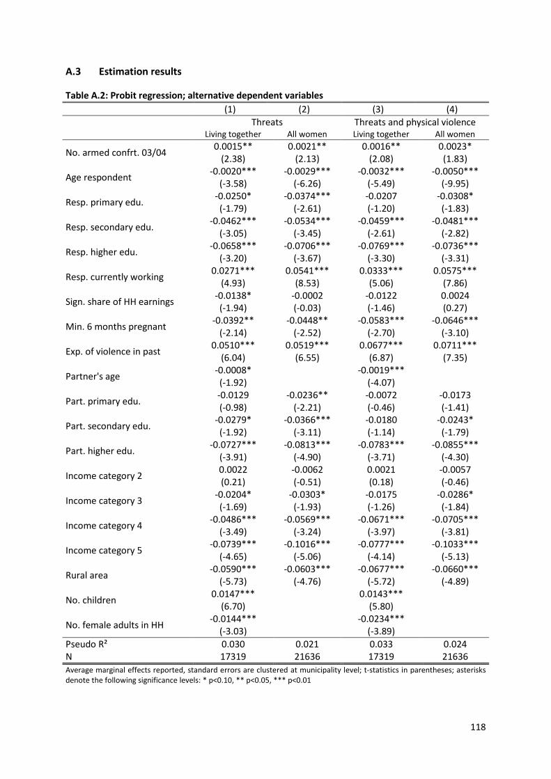
118

A.3 Estimation results

Table A.2: Probit regression; alternative dependent variables (1) (2) (3) (4)

Threats Threats and physical violence

Living together All women Living together All women

No. armed confrt. 03/04 0.0015** 0.0021** 0.0016** 0.0023* (2.38) (2.13) (2.08) (1.83)

Age respondent -0.0020*** -0.0029*** -0.0032*** -0.0050*** (-3.58) (-6.26) (-5.49) (-9.95)

Resp. primary edu. -0.0250* -0.0374*** -0.0207 -0.0308* (-1.79) (-2.61) (-1.20) (-1.83)

Resp. secondary edu. -0.0462*** -0.0534*** -0.0459*** -0.0481*** (-3.05) (-3.45) (-2.61) (-2.82)

Resp. higher edu. -0.0658*** -0.0706*** -0.0769*** -0.0736*** (-3.20) (-3.67) (-3.30) (-3.31)

Resp. currently working 0.0271*** 0.0541*** 0.0333*** 0.0575*** (4.93) (8.53) (5.06) (7.86)

Sign. share of HH earnings -0.0138* -0.0002 -0.0122 0.0024 (-1.94) (-0.03) (-1.46) (0.27)

Min. 6 months pregnant -0.0392** -0.0448** -0.0583*** -0.0646*** (-2.14) (-2.52) (-2.70) (-3.10)

Exp. of violence in past 0.0510*** 0.0519*** 0.0677*** 0.0711*** (6.04) (6.55) (6.87) (7.35)

Partner's age -0.0008*

-0.0019*** (-1.92)

(-4.07)

Part. primary edu. -0.0129 -0.0236** -0.0072 -0.0173 (-0.98) (-2.21) (-0.46) (-1.41)

Part. secondary edu. -0.0279* -0.0366*** -0.0180 -0.0243* (-1.92) (-3.11) (-1.14) (-1.79)

Part. higher edu. -0.0727*** -0.0813*** -0.0783*** -0.0855*** (-3.91) (-4.90) (-3.71) (-4.30)

Income category 2 0.0022 -0.0062 0.0021 -0.0057 (0.21) (-0.51) (0.18) (-0.46)

Income category 3 -0.0204* -0.0303* -0.0175 -0.0286* (-1.69) (-1.93) (-1.26) (-1.84)

Income category 4 -0.0486*** -0.0569*** -0.0671*** -0.0705*** (-3.49) (-3.24) (-3.97) (-3.81)

Income category 5 -0.0739*** -0.1016*** -0.0777*** -0.1033*** (-4.65) (-5.06) (-4.14) (-5.13)

Rural area -0.0590*** -0.0603*** -0.0677*** -0.0660*** (-5.73) (-4.76) (-5.72) (-4.89)

No. children 0.0147***

0.0143*** (6.70)

(5.80)

No. female adults in HH -0.0144***

-0.0234*** (-3.03)

(-3.89)

Pseudo R² 0.030 0.021 0.033 0.024 N 17319 21636 17319 21636 Average marginal effects reported, standard errors are clustered at municipality level; t-statistics in parentheses; asterisks denote the following significance levels: * p<0.10, ** p<0.05, *** p<0.01

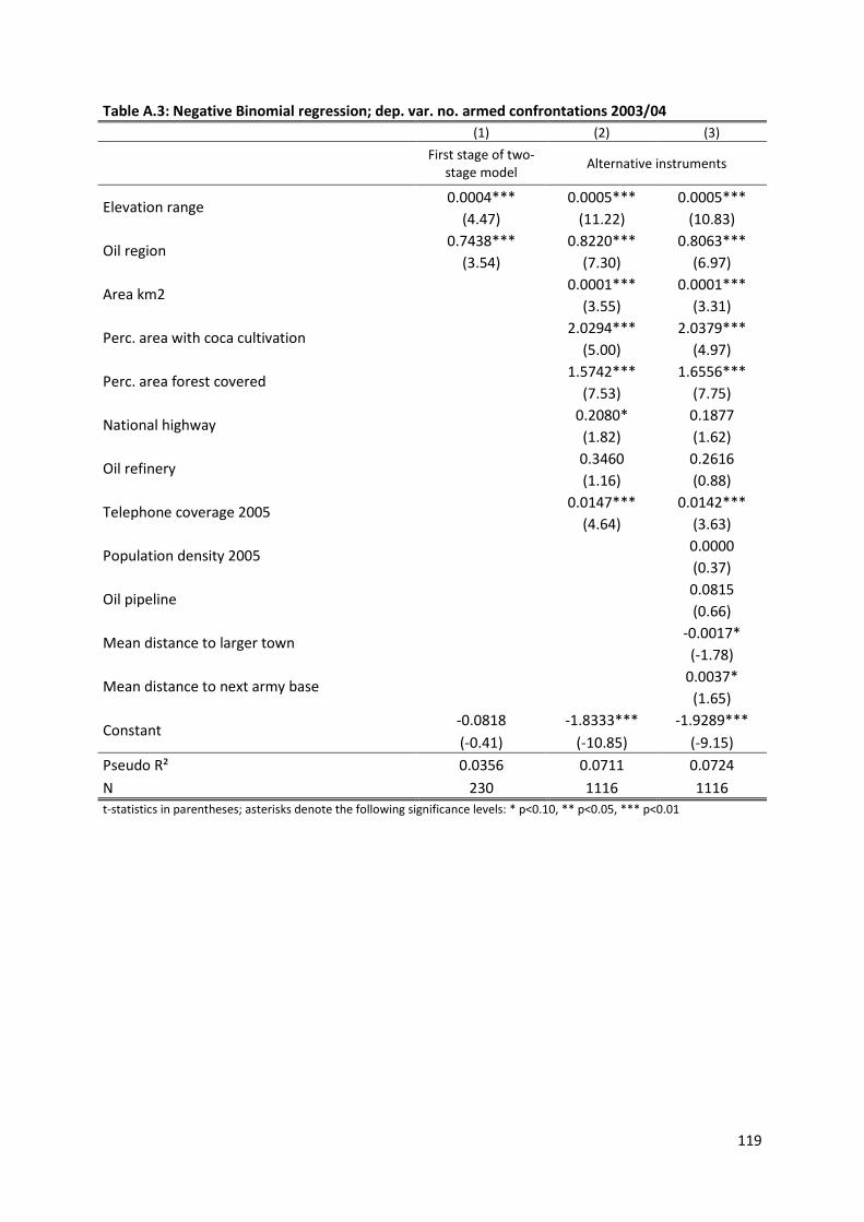
119

Table A.3: Negative Binomial regression; dep. var. no. armed confrontations 2003/04 (1) (2) (3)

First stage of two-

stage model Alternative instruments

Elevation range 0.0004*** 0.0005*** 0.0005*** (4.47) (11.22) (10.83)

Oil region 0.7438*** 0.8220*** 0.8063*** (3.54) (7.30) (6.97)

Area km2 0.0001*** 0.0001***

(3.55) (3.31)

Perc. area with coca cultivation 2.0294*** 2.0379***

(5.00) (4.97)

Perc. area forest covered 1.5742*** 1.6556***

(7.53) (7.75)

National highway 0.2080* 0.1877

(1.82) (1.62)

Oil refinery 0.3460 0.2616

(1.16) (0.88)

Telephone coverage 2005 0.0147*** 0.0142***

(4.64) (3.63)

Population density 2005 0.0000

(0.37)

Oil pipeline 0.0815

(0.66)

Mean distance to larger town -0.0017*

(-1.78)

Mean distance to next army base 0.0037*

(1.65)

Constant -0.0818 -1.8333*** -1.9289*** (-0.41) (-10.85) (-9.15)

Pseudo R² 0.0356 0.0711 0.0724 N 230 1116 1116 t-statistics in parentheses; asterisks denote the following significance levels: * p<0.10, ** p<0.05, *** p<0.01

120

A.4 Geography

Figure A.1: Surveyed districts in Colombia

Source: Authors’ calculations. DHS Data: Profamilia (2005); Map data for Colombian districts: SIG-OT (2013);

Map data for neighbouring features: DIVA-GIS (2013).

121

Figure A.2: Conflict intensity

Source: Authors’ calculations. Conflict data: Programa Presidencial de Derechos Humanos y Derecho

Internacional Humanitario (2010); Map data for Colombian districts: SIG-OT (2013); Map data for neighbouring

features: DIVA-GIS (2013).

122

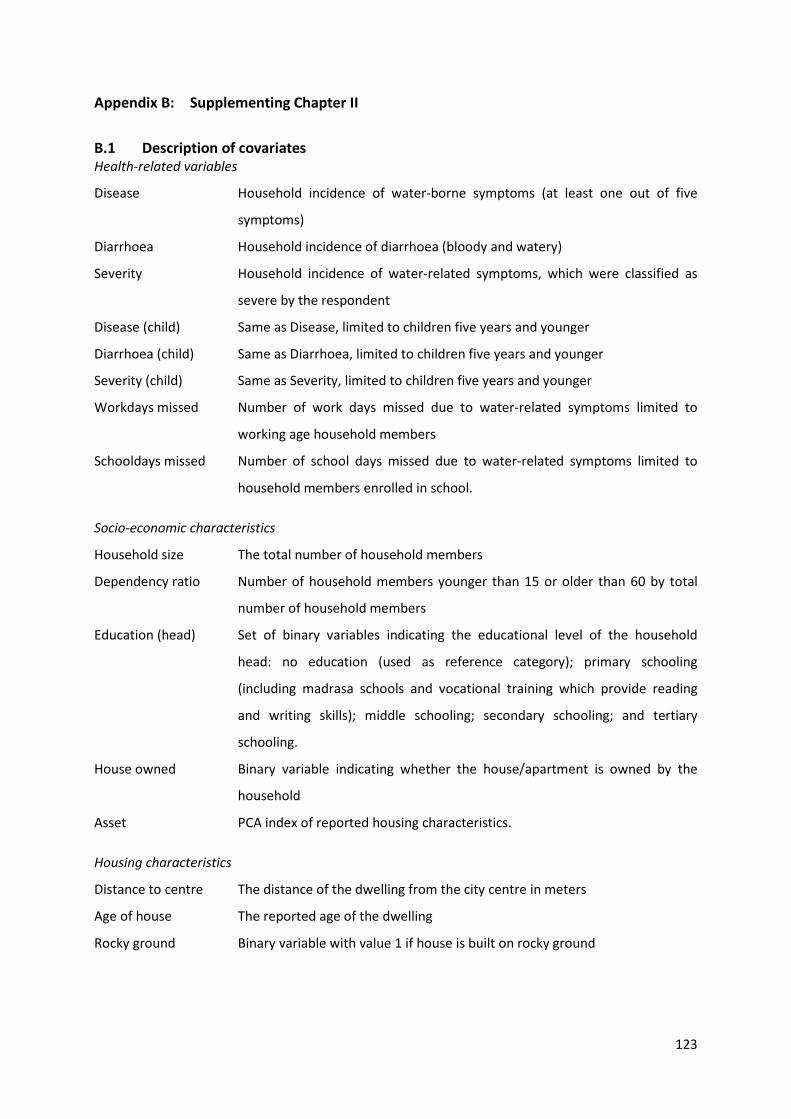
123

Appendix B: Supplementing Chapter II

B.1 Description of covariates Health-related variables

Disease Household incidence of water-borne symptoms (at least one out of five

symptoms)

Diarrhoea Household incidence of diarrhoea (bloody and watery)

Severity Household incidence of water-related symptoms, which were classified as

severe by the respondent

Disease (child) Same as Disease, limited to children five years and younger

Diarrhoea (child) Same as Diarrhoea, limited to children five years and younger

Severity (child) Same as Severity, limited to children five years and younger

Workdays missed Number of work days missed due to water-related symptoms limited to

working age household members

Schooldays missed Number of school days missed due to water-related symptoms limited to

household members enrolled in school.

Socio-economic characteristics

Household size The total number of household members

Dependency ratio Number of household members younger than 15 or older than 60 by total

number of household members

Education (head) Set of binary variables indicating the educational level of the household

head: no education (used as reference category); primary schooling

(including madrasa schools and vocational training which provide reading

and writing skills); middle schooling; secondary schooling; and tertiary

schooling.

House owned Binary variable indicating whether the house/apartment is owned by the

household

Asset PCA index of reported housing characteristics.

Housing characteristics

Distance to centre The distance of the dwelling from the city centre in meters

Age of house The reported age of the dwelling

Rocky ground Binary variable with value 1 if house is built on rocky ground

124

Hygiene-related variables

Knowledge (disease) Binary variable, takes the value 1 if the health knowledge question correctly

answered. Test asks about five symptoms of water borne diseases

Soap Binary variable indicating whether soap and/or detergent is used for hand

washing

Purification Binary variable indicating whether water is purified by the household before

drinking

Water quality-related variables

Unreliable Binary variable indicating whether the respondent claimed that the most

substantial problem of the main source for drinking water is unreliability

Bad water quality Binary variable indicating whether the quality of the water from the main

source for drinking is „bad“ or „very bad“; self-reported

Sewerage clogging Number of times the toilet of the household was unusable during the past

three months

Truck Binary variable indicating whether household uses trucked water for drinking

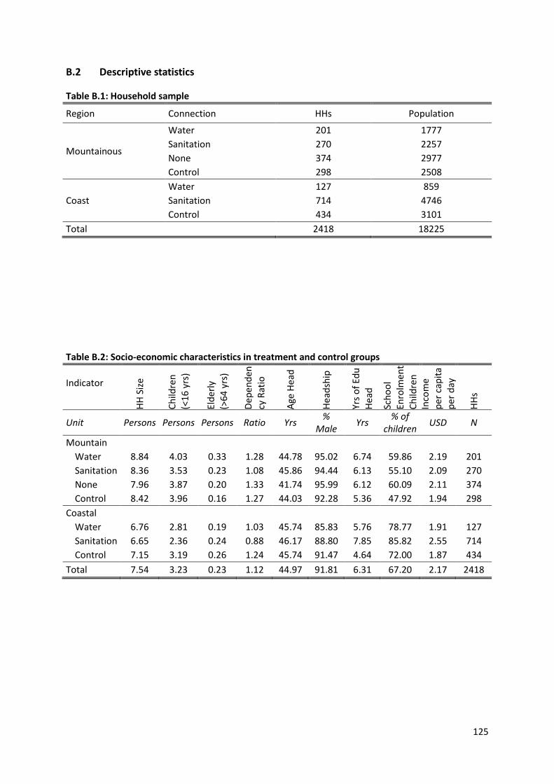
125

B.2 Descriptive statistics

Table B.1: Household sample

Region Connection HHs Population

Mountainous

Water 201 1777 Sanitation 270 2257 None 374 2977 Control 298 2508

Coast Water 127 859 Sanitation 714 4746 Control 434 3101

Total 2418 18225

Table B.2: Socio-economic characteristics in treatment and control groups

Indicator

HH S

ize

Child

ren

(<

16 y

rs)

Elde

rly

(>64

yrs

)

Depe

nden

cy R

atio

Age

Head

Head

ship

Yrs o

f Edu

He

ad

Scho

ol

Enro

lmen

t Ch

ildre

n In

com

e pe

r cap

ita

per d

ay

HHs

Unit Persons Persons Persons Ratio Yrs % Male Yrs % of

children USD N

Mountain Water 8.84 4.03 0.33 1.28 44.78 95.02 6.74 59.86 2.19 201 Sanitation 8.36 3.53 0.23 1.08 45.86 94.44 6.13 55.10 2.09 270 None 7.96 3.87 0.20 1.33 41.74 95.99 6.12 60.09 2.11 374 Control 8.42 3.96 0.16 1.27 44.03 92.28 5.36 47.92 1.94 298 Coastal Water 6.76 2.81 0.19 1.03 45.74 85.83 5.76 78.77 1.91 127 Sanitation 6.65 2.36 0.24 0.88 46.17 88.80 7.85 85.82 2.55 714 Control 7.15 3.19 0.26 1.24 45.74 91.47 4.64 72.00 1.87 434 Total 7.54 3.23 0.23 1.12 44.97 91.81 6.31 67.20 2.17 2418

126

Table B.3: Contamination of drinking cup

Region Connection Well type e.coli HH

% N

Mountainous

Water Pipewells

20.0 70.0 Sanitation 38.4 73.0 None Truckwells 20.3 64.0 Control Truckwells 40.0 65.0

Coastal

Water Pipewells

46.4 69.0 Water & Sanit. 36.6 71.0 Control Truckwells 61.4 88.0

Total 38.6 500.0

Table B.4: Change of pollution between storage tank and drinking cup

Region Connection e.coli HH

Percentage Points N

Mountainous Water 23.3 116 No Connection 16 50 Control 22 50

Coastal Water 25.6 117 Control 31 71

Total 24.1 407

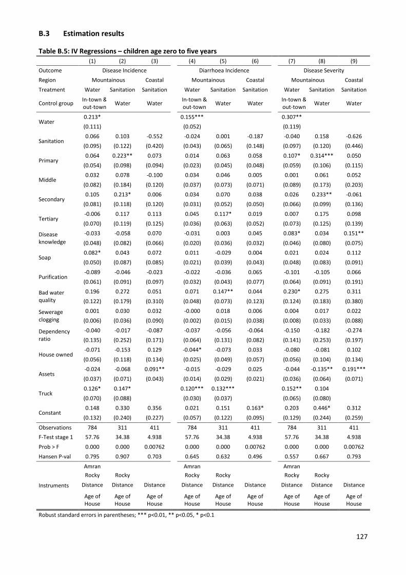
127

B.3 Estimation results

Table B.5: IV Regressions – children age zero to five years (1) (2) (3) (4) (5) (6) (7) (8) (9) Outcome Disease Incidence Diarrhoea Incidence Disease Severity Region Mountainous Coastal Mountainous Coastal Mountainous Coastal Treatment Water Sanitation Sanitation Water Sanitation Sanitation Water Sanitation Sanitation

Control group In-town & out-town Water Water In-town &

out-town Water Water In-town & out-town Water Water

Water 0.213* 0.155*** 0.307** (0.111) (0.052) (0.119)

Sanitation 0.066 0.103 -0.552 -0.024 0.001 -0.187 -0.040 0.158 -0.626

(0.095) (0.122) (0.420) (0.043) (0.065) (0.148) (0.097) (0.120) (0.446)

Primary 0.064 0.223** 0.073 0.014 0.063 0.058 0.107* 0.314*** 0.050

(0.054) (0.098) (0.094) (0.023) (0.045) (0.048) (0.059) (0.106) (0.115)

Middle 0.032 0.078 -0.100 0.034 0.046 0.005 0.001 0.061 0.052

(0.082) (0.184) (0.120) (0.037) (0.073) (0.071) (0.089) (0.173) (0.203)

Secondary 0.105 0.213* 0.006 0.034 0.070 0.038 0.026 0.233** -0.061

(0.081) (0.118) (0.120) (0.031) (0.052) (0.050) (0.066) (0.099) (0.136)

Tertiary -0.006 0.117 0.113 0.045 0.117* 0.019 0.007 0.175 0.098 (0.070) (0.119) (0.125) (0.036) (0.063) (0.052) (0.073) (0.125) (0.139)

Disease knowledge

-0.033 -0.058 0.070 -0.031 0.003 0.045 0.083* 0.034 0.151**

(0.048) (0.082) (0.066) (0.020) (0.036) (0.032) (0.046) (0.080) (0.075)

Soap 0.082* 0.043 0.072 0.011 -0.029 0.004 0.021 0.024 0.112 (0.050) (0.087) (0.085) (0.021) (0.039) (0.043) (0.048) (0.083) (0.091)

Purification -0.089 -0.046 -0.023 -0.022 -0.036 0.065 -0.101 -0.105 0.066 (0.061) (0.091) (0.097) (0.032) (0.043) (0.077) (0.064) (0.091) (0.191)

Bad water quality

0.196 0.272 0.051 0.071 0.147** 0.044 0.230* 0.275 0.311

(0.122) (0.179) (0.310) (0.048) (0.073) (0.123) (0.124) (0.183) (0.380)

Sewerage clogging

0.001 0.030 0.032 -0.000 0.018 0.006 0.004 0.017 0.022 (0.006) (0.036) (0.090) (0.002) (0.015) (0.038) (0.008) (0.033) (0.088)

Dependency ratio

-0.040 -0.017 -0.087 -0.037 -0.056 -0.064 -0.150 -0.182 -0.274 (0.135) (0.252) (0.171) (0.064) (0.131) (0.082) (0.141) (0.253) (0.197)

House owned -0.071 -0.153 0.129 -0.044* -0.073 0.033 -0.080 -0.081 0.102

(0.056) (0.118) (0.134) (0.025) (0.049) (0.057) (0.056) (0.104) (0.134)

Assets -0.024 -0.068 0.091** -0.015 -0.029 0.025 -0.044 -0.135** 0.191*** (0.037) (0.071) (0.043) (0.014) (0.029) (0.021) (0.036) (0.064) (0.071)

Truck 0.126* 0.147* 0.120*** 0.132*** 0.152** 0.104 (0.070) (0.088) (0.030) (0.037) (0.065) (0.080)

Constant 0.148 0.330 0.356 0.021 0.151 0.163* 0.203 0.446* 0.312

(0.132) (0.240) (0.227) (0.057) (0.122) (0.095) (0.129) (0.244) (0.259)

Observations 784 311 411 784 311 411 784 311 411 F-Test stage 1 57.76 34.38 4.938 57.76 34.38 4.938 57.76 34.38 4.938

Prob > F 0.000 0.000 0.00762 0.000 0.000 0.00762 0.000 0.000 0.00762 Hansen P-val 0.795 0.907 0.703 0.645 0.632 0.496 0.557 0.667 0.793

Instruments

Amran Amran Amran Rocky

d Rocky

d Rocky

d Rocky

d Rocky

d Rocky

d

Distance

Distance

Distance C

Distance

Distance C

Distance C

Distance

Distance C

Distance

Age of House

Age of House

Age of House Age of

House Age of House

Age of House Age of

House Age of House

Age of House

Robust standard errors in parentheses; *** p<0.01, ** p<0.05, * p<0.1

128

Table B.6: IV Regressions – all ages (1) (2) (3) (4) (5) (6) (7) (8) (9) Outcome Disease Incidence Diarrhoea Incidence Disease Severity Region Mountain Coastal Mountain Coastal Mountain Coastal Treatment Water Sanitation Sanitation Water Sanitation Sanitation Water Sanitation Sanitation

Control group In-town & out-town Water Water In-town &

out-town Water Water In-town & out-town Water Water

Water 0.072** 0.035 0.067** (0.031) (0.022) (0.027)

Sanitation -0.012 0.008 -0.152 0.002 0.011 -0.071 -0.022 0.024 -0.079 (0.025) (0.028) (0.122) (0.017) (0.021) (0.096) (0.022) (0.026) (0.083)

Primary -0.003 0.036* -0.002 0.010 0.026* -0.006 -0.004 0.029 -0.010 (0.012) (0.021) (0.016) (0.008) (0.014) (0.010) (0.011) (0.019) (0.013)

Middle -0.003 -0.034 0.014 0.010 -0.000 0.027 -0.023 -0.029 0.002

(0.019) (0.028) (0.035) (0.013) (0.019) (0.028) (0.015) (0.024) (0.025) Secondary 0.014 0.038 -0.006 0.023* 0.030 0.009 -0.003 0.028 -0.019

(0.018) (0.027) (0.019) (0.013) (0.019) (0.014) (0.015) (0.022) (0.016) Tertiary -0.002 0.023 0.018 0.025 0.047 0.008 -0.011 0.010 -0.003

(0.021) (0.039) (0.023) (0.016) (0.031) (0.017) (0.018) (0.032) (0.019) Disease knowledge

0.005 -0.005 0.017 0.002 0.014 0.010 0.025*** 0.016 0.016*

(0.011) (0.018) (0.012) (0.008) (0.013) (0.008) (0.009) (0.015) (0.010) Soap 0.014 -0.004 0.036** 0.011 0.001 0.007 0.004 -0.000 0.017

(0.012) (0.020) (0.017) (0.008) (0.013) (0.012) (0.010) (0.018) (0.013) Purification -0.006 0.003 0.097 -0.010 -0.011 0.062 -0.010 -0.013 0.058

(0.015) (0.022) (0.060) (0.011) (0.016) (0.045) (0.012) (0.018) (0.046) Bad water quality

0.042 0.034 0.023 0.030 0.027 0.007 0.040* 0.027 0.048

(0.026) (0.035) (0.041) (0.021) (0.028) (0.037) (0.021) (0.028) (0.039) Sewerage clogging

0.002 0.008 0.009 0.000 0.010 0.007 0.001 0.001 -0.003 (0.002) (0.008) (0.007) (0.001) (0.007) (0.007) (0.001) (0.005) (0.005)

Dependency ratio

0.121*** 0.113* 0.046 0.052** 0.054 0.023 0.100*** 0.103* 0.044 (0.037) (0.063) (0.034) (0.025) (0.046) (0.023) (0.034) (0.056) (0.029)

House owned -0.044*** -0.057* -0.006 -0.014 -0.031 -0.002 -0.028** -0.028 0.014

(0.014) (0.029) (0.027) (0.010) (0.019) (0.021) (0.012) (0.024) (0.017) Assets -0.009 -0.010 0.019* -0.004 -0.000 0.016** -0.013* -0.018 0.018**

(0.009) (0.018) (0.011) (0.007) (0.014) (0.007) (0.007) (0.014) (0.008) Truck 0.025 0.025 0.038*** 0.044*** 0.019 0.021

(0.017) (0.020) (0.010) (0.013) (0.015) (0.017) Constant 0.022 0.077 0.114 -0.026 -0.010 0.043 0.022 0.044 0.038

(0.030) (0.057) (0.073) (0.023) (0.046) (0.056) (0.026) (0.048) (0.050) Observations 1,072 436 826 1,072 436 826 1,072 436 826

F-Test stage 1 78.71 46.91 3.160 78.71 46.91 3.160 78.71 46.91 3.160 Prob > F 0.000 0.000 0.043 0.000 0.000 0.043 0.000 0.000 0.043 Hansen P-val 0.561 0.887 0.330 0.380 0.335 0.420 0.294 0.518 0.792

Instruments

Amran Amran Amran Rocky

G d Rocky

G d Rocky

G d Rocky

G d Rocky

G d Rocky

G d

Distance

Distance

Distance

Distance

Distance

Distance

Distance

Distance

Distance Age of

Age of

Age of

Age of

Age of

Age of

Age of

Age of

Age of

Robust standard errors in parentheses; *** p<0.01, ** p<0.05, * p<0.1

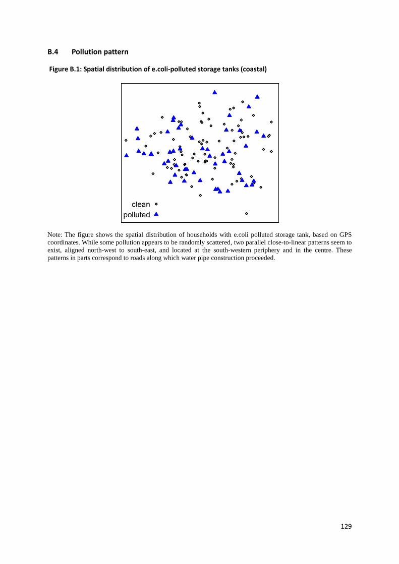
129

B.4 Pollution pattern

Figure B.1: Spatial distribution of e.coli-polluted storage tanks (coastal)

Note: The figure shows the spatial distribution of households with e.coli polluted storage tank, based on GPS coordinates. While some pollution appears to be randomly scattered, two parallel close-to-linear patterns seem to exist, aligned north-west to south-east, and located at the south-western periphery and in the centre. These patterns in parts correspond to roads along which water pipe construction proceeded.

130

131

Appendix C: Supplementing Chapter III

C.1 Technical notes

Methods of water purification differ in their capability to withhold or neutralize different

contaminations (viruses, bacteria, vermin, chemicals, excess or harmful minerals like arsenic or

fluorides, and suspended particles), their speed of use and suitability for different volumes, and their

effectiveness to improve colour, odour and taste of the water. These methods include domestic

chemical disinfection using chlorine or iodine, boiling, filtration, pre-settlement before use, storage

and sedimentation, a coagulation-flocculation-settlement-procedure, aeration, exposure to sunlight,

and desalination (see Brikké, Bredero 2003Brikké and Bredero, 2003). Below, I summarize the most

important details regarding these methods.

While chlorination is easy and cost-efficient, its drawback is its unsavoury taste. The chlorine can be

added in form of powder, tablets or liquid. Chlorine compounds immediately start to react with

pathogen in the water. If enough chlorine was added, some free residual chlorine will remain

detectable after all pathogens have been destroyed. A concentration of 0.5 milligram per litre is

recommended (World Health Organization, 2008) in order to secure continued disinfection in case

new pathogens enter, while higher concentrations will shift the trade-off between disinfection and

taste to the detriment of the latter. Initial water quality – including turbidity – commands the

amount of chlorine needed. Iodine has a similar effect, while the taste is perceived by many users to

be less offensive, especially when adding vitamin C to the water following the contact time.

Nonetheless, water treated with iodine is not recommended for consumption for pregnant women

and persons allergic to iodine.

Boiling reliably kills off microorganisms causing diarrheal diseases, even at high altitudes with low air

pressure and a lowered boiling point of the water. As the effect is reached already below the boiling

point, even short ebullition is sufficient.

Filtration works through particle removal or adsorption. Several methods are available, differing in

level of sophistication, cost and speed. These include slow and rapid sand filtration, straining through

fine cloth, ceramic filters, silver-ion filters, membrane and reverse osmosis processes, combined

technology filtration, and adsorption using granular charcoal or activated carbon filters.

Simple presettlement of the drinking water for more than two days eliminates besides some bacteria

also Carcaria snail larvae, for example. Longer storage and sedimentation is a method rather used at

communal than at domestic level due to the rather time-consuming character of the procedure,

which makes it inconvenient for day-to-day application. Solid contaminants sink to the ground of the

storage container and can then be separated from the drinking water. When employing the

132

coagulation-flocculation-settlement-procedure, a liquid coagulant is intermixed with the water in

order to bind particles. These then cohere to larger flocks and collect at the ground or can be

removed otherwise. Aluminium sulphate is an example for a suitable coagulant. Aeration oxidizes

iron and manganese.

Exposure to sunlight in a clear plastic – not glass – bottle to direct ultraviolet rays will kill the majority

of microbes in the water within a couple of hours. The method is sometimes referred to as solar

water disinfection (SODIS).

Desalination alleviates disinfection due to “low total organic carbon and particle content, low

microbial loads and minimal oxidant demand” (Curtis, Cairncross 2003), but should be combined with

chlorination.

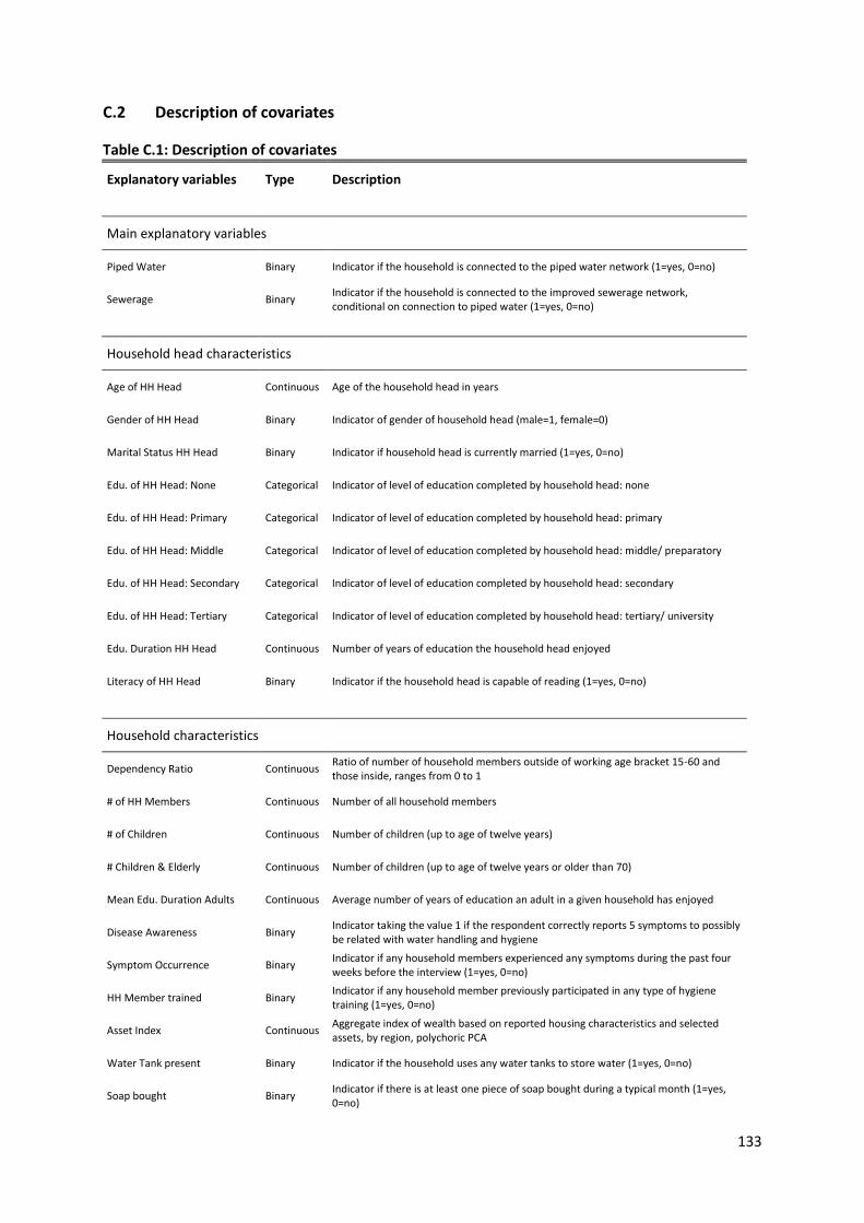
133

C.2 Description of covariates

Table C.1: Description of covariates

Explanatory variables Type Description

Main explanatory variables

Piped Water Binary Indicator if the household is connected to the piped water network (1=yes, 0=no)

Sewerage Binary Indicator if the household is connected to the improved sewerage network, conditional on connection to piped water (1=yes, 0=no)

Household head characteristics

Age of HH Head Continuous Age of the household head in years

Gender of HH Head Binary Indicator of gender of household head (male=1, female=0)

Marital Status HH Head Binary Indicator if household head is currently married (1=yes, 0=no)

Edu. of HH Head: None Categorical Indicator of level of education completed by household head: none

Edu. of HH Head: Primary Categorical Indicator of level of education completed by household head: primary

Edu. of HH Head: Middle Categorical Indicator of level of education completed by household head: middle/ preparatory

Edu. of HH Head: Secondary Categorical Indicator of level of education completed by household head: secondary

Edu. of HH Head: Tertiary Categorical Indicator of level of education completed by household head: tertiary/ university

Edu. Duration HH Head Continuous Number of years of education the household head enjoyed

Literacy of HH Head Binary Indicator if the household head is capable of reading (1=yes, 0=no)

Household characteristics

Dependency Ratio Continuous Ratio of number of household members outside of working age bracket 15-60 and those inside, ranges from 0 to 1

# of HH Members Continuous Number of all household members

# of Children Continuous Number of children (up to age of twelve years)

# Children & Elderly Continuous Number of children (up to age of twelve years or older than 70)

Mean Edu. Duration Adults Continuous Average number of years of education an adult in a given household has enjoyed

Disease Awareness Binary Indicator taking the value 1 if the respondent correctly reports 5 symptoms to possibly be related with water handling and hygiene

Symptom Occurrence Binary Indicator if any household members experienced any symptoms during the past four weeks before the interview (1=yes, 0=no)

HH Member trained Binary Indicator if any household member previously participated in any type of hygiene training (1=yes, 0=no)

Asset Index Continuous Aggregate index of wealth based on reported housing characteristics and selected assets, by region, polychoric PCA

Water Tank present Binary Indicator if the household uses any water tanks to store water (1=yes, 0=no)

Soap bought Binary Indicator if there is at least one piece of soap bought during a typical month (1=yes, 0=no)

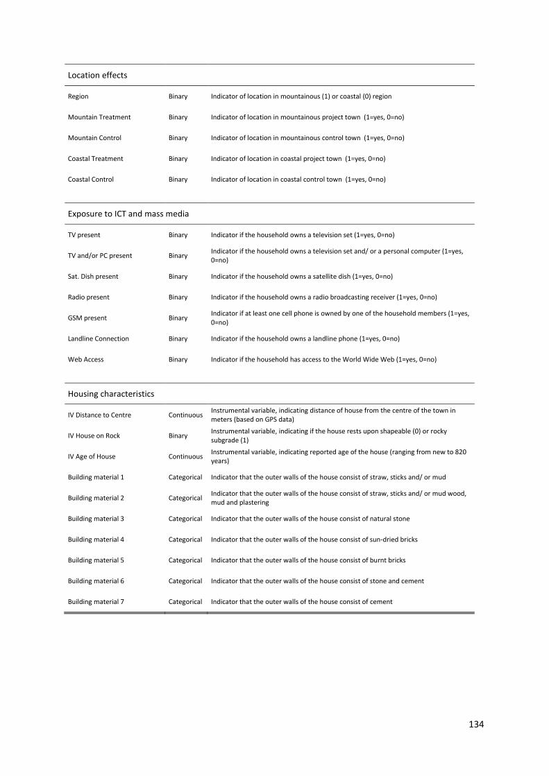
134

Location effects

Region Binary Indicator of location in mountainous (1) or coastal (0) region

Mountain Treatment Binary Indicator of location in mountainous project town (1=yes, 0=no)

Mountain Control Binary Indicator of location in mountainous control town (1=yes, 0=no)

Coastal Treatment Binary Indicator of location in coastal project town (1=yes, 0=no)

Coastal Control Binary Indicator of location in coastal control town (1=yes, 0=no)

Exposure to ICT and mass media

TV present Binary Indicator if the household owns a television set (1=yes, 0=no)

TV and/or PC present Binary Indicator if the household owns a television set and/ or a personal computer (1=yes, 0=no)

Sat. Dish present Binary Indicator if the household owns a satellite dish (1=yes, 0=no)

Radio present Binary Indicator if the household owns a radio broadcasting receiver (1=yes, 0=no)

GSM present Binary Indicator if at least one cell phone is owned by one of the household members (1=yes, 0=no)

Landline Connection Binary Indicator if the household owns a landline phone (1=yes, 0=no)

Web Access Binary Indicator if the household has access to the World Wide Web (1=yes, 0=no)

Housing characteristics

IV Distance to Centre Continuous Instrumental variable, indicating distance of house from the centre of the town in meters (based on GPS data)

IV House on Rock Binary Instrumental variable, indicating if the house rests upon shapeable (0) or rocky subgrade (1)

IV Age of House Continuous Instrumental variable, indicating reported age of the house (ranging from new to 820 years)

Building material 1 Categorical Indicator that the outer walls of the house consist of straw, sticks and/ or mud

Building material 2 Categorical Indicator that the outer walls of the house consist of straw, sticks and/ or mud wood, mud and plastering

Building material 3 Categorical Indicator that the outer walls of the house consist of natural stone

Building material 4 Categorical Indicator that the outer walls of the house consist of sun-dried bricks

Building material 5 Categorical Indicator that the outer walls of the house consist of burnt bricks

Building material 6 Categorical Indicator that the outer walls of the house consist of stone and cement

Building material 7 Categorical Indicator that the outer walls of the house consist of cement

135

C.3 Descriptive statistics

Table C.2: Means and differences of outcomes by connection status Outcome Mean, not

connected (control)

Min Max Mean, piped water

Min Max Diff. to control

Mean, improved sewerage

Min Max Diff. to control

1) Treatment of drinking water 0.069 0 1 0.120 0 1 0.050*** 0.107 0 1 0.037***

2) Use of cleanser for hand washing 0.614 0 1 0.695 0 1 0.083*** 0.820 0 1 0.208***

3) Spending for soap 64.85 0 500 84.46 0 428.89 19.61*** 82.97 0 500 18.12***

4) Spending for cleanser 144.78 0 760 149.42 0 562.50 4.64 162.88 0 833.33 18.10***

5) Frequency of latrine-cleaning 7.57 0 28 7.93 1 21 0.37* 8.38 0 35 0.82***

Table C.3: Mean spending (per capita, in YER) on cleanser by location and connection status

Connection Mountain

Project (YER)

N SD Mountain

Control (YER)

N SD Coastal

Project (YER)

N SD Coastal

Control (YER)

N SD

None 153.87 265 111.93 160.01 196 123.26 - - - 131.85 425 116.45

Piped Water 159.38 125 105.01 - - -

138.91 118 115.96 - - -

Sewerage 173.21 180 119.26 - - - 160.26 660 132.60 - - -

N over all connection groups and locations: 1969

Note: no households are connected to piped water or improved sewerage in the control towns. All households in the sample are connected in the coastal project town. Values capped at 500 YER per capita for each component (spending on soap, spending on laundry detergent) to exclude industrial use.

136

C.4 Methodology of employed instrumental variable approaches

I briefly summarize the findings on relevance and validity of the instrumental variables considered

for use in Chapter III. For the dependent variable Probability of Drinking Water Treatment, the

instruments IV Age of House and IV Rocky Ground used in the Wooldridge procedure (which is

explained below) appear valid with F-statistics of the predicted values well above the critical value115

for both (separately) instrumented covariates. Exogeneity is more of a concern, as the Sargan-

Hansen test for overidentification suggests that the null hypothesis – which says that the instrument

or set of instruments is valid – can be rejected on grounds of statistical significance116 at the

conventional level of five (when instrumenting Connection to Piped Water) respectively ten

(Connection to Improved Sewerage) per cent.117 For the dependent variable Use of Cleanser for Hand

Washing the same two instruments appear valid, while the Sargan-Hansen test again does not

provide support for my assumption of exogeneity.118

For Spending on Soap the picture looks similarly unsatisfactory. The two instruments receive less

support regarding their validity now, while the null of exogeneity of the instruments can still be

rejected at the ten per cent level.119 When introducing the third instrument IV Distance on top of the

other two, validity is compellingly supported again; but lack of support of the assumption of

exogeneity by the Sargan-Hansen test remains an issue.120 For the more comprehensive Spending on

115 For the instrumented covariate Connection to Piped Water the Cragg-Donald Wald F-statistic is 36.90 compared to a Stock-Yogo critical reference value of 16.38 for one instrumented endogenous covariate and one instrument, and a desired size of a Wald test of 0.10 at a significance level of five per cent. For the covariate Connection to Improved Sewerage the F-statistic reads 30.54. Note that the two instruments are reduced to one in the Wooldridge procedure, namely the predicted value of the instrumented connection indicator. 116 Whenever I write about significance in the following and if not indicated otherwise, he refers to statistical significance at conventional levels. 117 The IV-Probit estimator obtains a p-value of 0.0448 for Connection to Piped Water respectively 0.0613 for Connection to Improved Sewerage. 118 For the instrumented covariate Connection to Piped Water the Cragg-Donald Wald F-statistic is 36.78 compared to a Stock-Yogo critical reference value of 16.38, with the same conditions applying as above. For the covariate Connection to Improved Sewerage the F-statistic reads 29.90. The IV-Probit estimator obtains a p-value of 0.0121 for Connection to Piped Water respectively 0.0006 for Connection to Improved Sewerage. 119 For the instrumented covariate Connection to Piped Water the Cragg-Donald Wald F-statistic is 10.47 compared to a Stock-Yogo critical reference value of 8.75, but only at a desired size of a Wald test of 0.20 (at a significance level of five per cent). For the covariate Connection to Improved Sewerage the F-statistic reads 8.08, compared to a reference value of 7.25 at a desired size of the Wald test of 0.25. 2SLS obtains a p-value of 0.0539 for Connection to Piped Water, and 0.0056 for Connection to Improved Sewerage, respectively regressed on two instruments. 120 For the instrumented covariate Connection to Piped Water – and now three instead of two instruments – the Cragg-Donald Wald F-statistic is 91.19 compared to a Stock-Yogo critical reference value of 13.91 at a desired size of a Wald test of 0.05 (at a significance level of five per cent). For Connection to Improved

137

Cleanser not much does change. Including only two of the three instruments leads to lower F-

statistics, as before. With the full set of three instruments, though, validity is strongly supported.121

The assumption of exogeneity still cannot be defended based on the Sargan-Hansen test,

interestingly even less so when including the third instrument.122

When looking at the fifth and last outcome of interest – Frequency of Latrine-Cleaning – the pattern

remains the same as with the two continuous expenditure variables before: validity can better be

supported when including three instrumental variables, while the statistical evidence raising doubts

about exogeneity is further diminished.123

The instruments chosen can be shown to be correlated with the decision to connect households to

the piped water network respectively additionally to the sewerage network, while most likely not

having an influence on probability of water treatment within the household or one of the other

outcomes. I judge that none of the three instrumental variables can in any way be linked on grounds

of rational argumentation with the outcome variables, as no transmission channels appear

conceivable. Still, the difficulties to reject endogeneity of the instruments based on statistical tests

create some concerns that the exclusion restriction might not be fulfilled. The results of the IV

estimations therefore should be regarded with some caution.

While the instruments are employed in this analysis also with a linear-binary and a simultaneous

maximum likelihood estimator (MLE) as well as with a two-stage Probit bootstrap (2SPrB) procedure,

Sewerage, the F-statistic reads 83.71. 2SLS obtains a p-value of 0.0046 for Connection to Piped Water and 0.0036 for Connection to Improved Sewerage, respectively regressed on three instruments. 121 For the instrumented covariate Connection to Piped Water the Cragg-Donald Wald F-statistic is 12.01 compared to a Stock-Yogo critical reference value of 11.59 at a desired size of a Wald test of 0.15 (at a significance level of five per cent), for two instruments. When including the third instrument the F-statistic rises to 84.27, which exceed the reference value of 13.91 for a Wald test size of 0.05. For Connection to Improved Sewerage and two instruments, the F-statistic reads 5.98, which is not even sufficient for a Wald test size of 0.25. When including the third instrument, the F-statistic rises to 77.59. 122 2SLS obtains a p-value of 0.0984 for Connection to Piped Water and 0.0237 for Connection to Improved Sewerage, respectively regressed on two instruments. When including the third instrument, the numbers change to 0.0012 and 0.0013, respectively. 123 For the instrumented covariate Connection to Piped Water the Cragg-Donald Wald F-statistic is 9.98 compared to a Stock-Yogo critical reference value of 8.75 at a desired size of a Wald test of 0.20 (at a significance level of five per cent), for two instruments. When including the third instrument the F-statistic rises to 92.48, which exceed the reference value of 13.91 for a Wald test size of 0.05. For Connection to Improved Sewerage and two instruments, the F-statistic reads 6.76, which is not even sufficient for a Wald test size of 0.25. When including the third instrument, the F-statistic rises to 84.00. 2SLS obtains a p-value of 0.0995 for Connection to Piped Water and 0.07984for Connection to Improved Sewerage, respectively regressed on two instruments. When including the third instrument, the numbers change to 0.0021 and 0.0034, respectively.

138

the two-stage IV estimation shall serve as example to explain the mode of operation. For the first

stage envision a linear probability model taking the form

�̂�𝑖𝑗 = 𝛼𝑖1 + 𝛽𝑖1′ 𝐻𝑗′ + 𝛾𝑖1′ 𝐸𝑗′ + 𝛿𝑖1′ 𝑍𝑗′ + 𝜇𝑖𝑗 (C.1)

where �̂�𝑖𝑗 indicates the predicted connection status i (piped water, sewerage) of each household j (C

stands for Connection). The dependent variable is estimated based on a vector of characteristics of

the head of the household (H stands for Household Head Characteristics), a vector of characteristics

of the household itself as a whole (E stands for Environment) including location and ICT exposure

measures, and a vector composed of the set of instrumental variables (Z stands for Instruments).

The constant is indicated by 𝛼1; 𝛽1, 𝛾1and 𝛿1 stand for the respective coefficients of the vector

variables of the first stage (subscript 1 stands for first stage). The error term 𝜇𝑗 varies non-

systematically over the observation units so that I can write the conditional expectation function

𝐸�𝜇𝑗 ∣ 𝐻𝑗′,𝐸𝑗′,𝑍𝑗′� = 0 (C.2)

In the second stage, I plug the predicted connection status �̂�𝑗 estimated in equation (1) into the

model estimating the dependent variable of interest. It takes the form

𝑂𝑑𝑗 = 𝛼2 + 𝛽2′𝐻𝑗′ + 𝛾2′𝐸𝑗′ + 𝛿𝑖2 �̂�𝑖𝑗 + 𝜀𝑗 (C.3)

with 𝑂𝑑𝑗 marking the reported behaviour of the household. O stands for Outcome; subscript d

(which stands for Dependent Variable) indicates whether the outcome estimated is 1) probability of

treatment of drinking water, 2) probability of using cleanser when washing hands, 3) logarithmised

per capita spending on soap or 4) a combination of soap and laundry detergent, or 5) the frequency

of latrine-cleaning. The other covariate vectors remain the same, the coefficients now marked with

subscript 2 for the second stage. 𝛼2 represents the constant, 𝜀𝑗 a non-systematic error term so that

– equivalent to equation (2) – I can write the conditional expectation function as

𝐸�𝜀𝑗 ∣ 𝐻𝑗′,𝐸𝑗′, �̂�𝑖𝑗� = 0 (C.4)

The fact that both the dependent variable as well as the main explanatory variable are binary

requires application of special estimators when trying to control for endogeneity. The choice of the

appropriate estimator is not straightforward. In the literature one can find an array of methods

applied. Each one comes with its assets and drawbacks, and no consensus on best practice has

emerged yet. Holm and Arendt (2012) state that, in opposition to ”models with continuous

endogenous repressors no simple consistent two-stage methods exist in the dummy endogenous

model”. They point out that 2SLS and Probit models will yield diverging estimates if something else

139

than average effects are calculated, or in presence of outliers. Rees et al. (2001) use various methods

as alternatives to a standard single-equation Probit estimator in order to allow for possible

endogeneity issues. These include maximum likelihood bivariate Probit as well as 2SLS instrumental

variable procedures. On the other hand, Angrist (2001) argues that nonlinear limited dependent

variables (LDV, as for example a binary positive outcome variable) models might only appear to

present particular difficulties regarding endogenous variables. He purports that causal inference in

presence of LDV outcomes is similar to that of continuous outcomes. At least when there are no or

“sparse and discrete” covariates, linear estimators are “no less appropriate for LDVs than for other

kinds of dependent variables”, he states.

In consideration of this lack of a widely accepted guideline I rely upon application of four estimation

procedures to control for endogeneity. This allows me to confidently peg and delineate the

conjectured range of coefficient size of the regressors. Besides a single-stage Probit estimator I

deploy the following instrumental variable procedures in the analysis at hand: 1) a particular form of

the bivariate Probit regression, 2) a two-stage Probit bootstrap regression, 3) a linear-binary

regression (IV-Probit) combined with a range-check; and as an entirely linear procedure 4) two-stage

least squares regression following a scheme as proposed by Wooldridge (2010). Below, these four

procedures are considered one by one, with a focus on the less commonly used bivariate Probit

estimator.

1) Bivariate Probit: Greene (2012) suggests that a model with an endogenous binary regressor can

be treated analogously to a selection problem. The two-step procedure developed by Heckman

(1978, see also Heckman, 1979, and Terza, 1986) is deemed inappropriate for application with a

Probit model by Freedman and Sekhon (2010), as it is assessed to frequently compound bias. Also it

is recognized to be inferior to maximum-likelihood procedures. They argue that under “ordinary

circumstances, the two-step-correction should not be used in Probit response models” because it

often increases bias. Carrasco (2001) chooses a bivariate Probit (otherwise also called Biprobit)

model to avoid the “inappropriateness of the standard instrumental variable method for analysing

the relationship between two endogenous discrete variables” in light of endogeneity. Chiburis, Das

and Lokshin (2011) find that Biprobit outperforms two-stage instrumental estimators for sample

sizes smaller than 5000, and when probability of treatment is close to the bounds of 0 and 1. They

also demonstrate that the MLE procedure allows calculating Average Treatment Effects (ATE).

140

This motivates the application of a simultaneous estimation procedure, namely the bivariate Probit

(Biprobit) estimator. The Biprobit procedure124 subdivides into three options, which fulfil different

functions. The regular bivariate Probit regression (BP) is according to Hardin (2012) suitable “for

models where the two dependent variables depend on the same list of independent variables and

are correlated”. The Seemingly Unrelated Biprobit regression (SUR BP) is applied when the

dependent variables of two equations ”may not depend on the same list of independent variables,

but are still correlated”, while the nested Probit regression is used “where the outcome of one

equation depends on the outcome of the other equation” (ibid.). The appropriate application in this

study – in order to instrument a binary and potentially endogenous regressor in combination with a

binary regressand – is a nested (or recursive, a label more commonly used in the literature) version

of the SUR BP. I refer to it in the following as RSUR BP. Park (2010) shows how to correctly125

formulate this RSUR BP model. Biprobit models assume that the error terms of the (simultaneously

estimated) equations are independent and identically distributed (see Greene, 2012). Independence

of the error terms and the instrumental variables is assumed.

The Biprobit estimators do not come without drawbacks, though. It is not appropriate when more

than one regressor is endogenous, or when an endogenous regressor interacts with an exogenous

one. The necessary assumptions regarding functional form and distributional considerations are

strong compared to those of other estimators.

The application of the Biprobit estimator requires two assumptions to be fulfilled. First, the variance

of the covariates must be sufficient (Dupas, 2011). The more restrictive assumption is the second:

the errors are assumed to be “distributed bivariate standard normal” (Davis et al., 2011); otherwise

the identification by functional form is problematic. This assumption can be tested using the Murphy

score test. In context of this study it turns out that the null hypotheses of bivariate standard normal

distribution is rejected for all tested specifications except for two cases where the probability of

drinking water treatment is regressed on connection to improved sewerage (test statistics are

available on request). The null is rejected for all Biprobit specifications regressing the probability of

cleanser use on any of the connection covariates; and for all those regressing the probability of

treatment of drinking water on connection to piped water. I therefore refrain from considering the

124 For details regarding the Biprobit estimator also refer to Maddala (1983) pp. 122-123 and Greene (2012), section 17.5, pp. 738 et sqq. 125 The correct STATA coding scheme presents oneself as biprobit (y = w x1-xn) (w = z x1-xn), with y denoting the binary outcome, x1-xn the exogenous regressors, w the potentially endogenous binary regressor, and z the instrumental variable or set of variables.

141

Biprobit to be a suitable estimator, but for purposes of documentation report the estimation results

in Appendix C.6 (columns labelled SUR BP, in Table C.11, Table C.12, Table C.15, and Table C.16).

2) Two-stage Probit bootstrap (2SPrB): an alternative estimation approach126 employed is similar to

that used by Noe and Rieckmann (2013). The difference is that I chose the Probit estimator for both

stages in the study at hand; instead of employing Negative Binomial estimator for the first stage and

a Probit estimator for the second. In the first stage the endogenous binary variable (henceforth

abbreviated EBV in this study, here the connection dummy) is regressed on the exogenous

covariates. In the second stage the outcome is regressed on the predicted value of the EBV and the

exogenous covariates. I employ bootstrapping127 to accurately calculate the standard errors, which

otherwise would in tendency be understated.

3) Linear-Binary (IV-Probit): I include the IV-Probit estimator for purpose of comparison, while

verifying128 upfront that the predicted value of the EBV regressed on instrumental variables and

exogenous covariates is not far beyond the lower and upper bounds of 0 and 1. The maximum-

likelihood option is preferred over the two-step option (i.e. the minimum chi-squared estimator

introduced by Newey, 1987) as no convergence problems are encountered, and is superior in terms

of efficiency. Note that some authors regard combining a linear model in the first stage with a

nonlinear model in the second stage not to be appropriate when the endogenous explanatory

variable is discrete (see, for example, Dong and Lewbel, 2012). Adkins (2009) point out (abbreviating

IV-Probit to IVP) that the “bias of IVP is substantial when instruments are weak”. Angrist and Pischke

(2008) explain that the IV-Probit estimator can, but does not have to be, superior to a 2SLS

approach.

4) Wooldridge Procedure (W2SLS): the two-stage least squares instrumental variable procedure (see

Turkington and Bowden, 1988, and Angrist and Krueger, 2001) may not be appropriate when the

dependent variable is binary (see Newey, 1987). 2SLS allows to estimate “local average causal

effects” (LATE, abbreviated alternatively ATT for Average Treatment effect on the Treated – see

Angrist and Pischke, 2008), but may be biased and inferior to MLE when handling small samples.

Wooldridge (2010)129 nonetheless proposes a three-step IV procedure to estimate the Average

126 This approach is based on an idea verbally suggested by Chris Müris. 127 The number of iterations chosen is 10,000. This is way beyond the 500 iterations used, for instance, by Bernheim et al. (2001), and allows confident estimation of the standard errors. 128 The two-stage IV-Probit procedure is here combined with an upstream range-check step using Ordinary Least Squares (OLS). This approach is based on a verbal suggestion given by Stephan Klasen. 129 See procedure 21.1, pp. 939 et seqq.

142

Treatment Effect (ATE), combining a Probit with a 2SLS regression. He advocates first regressing the

EBV on the set of exogenous covariates and the instrument, then in a second step predicting the

value of the EBV. In a third step, he then regresses the outcome on the set of exogenous covariates

and the EBV instrumented with its predicted value.

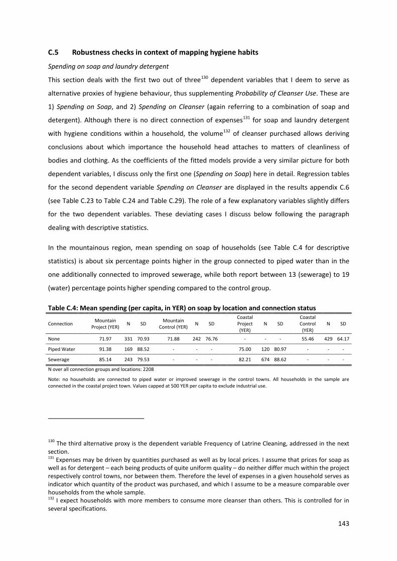
143

C.5 Robustness checks in context of mapping hygiene habits

Spending on soap and laundry detergent

This section deals with the first two out of three130 dependent variables that I deem to serve as

alternative proxies of hygiene behaviour, thus supplementing Probability of Cleanser Use. These are

1) Spending on Soap, and 2) Spending on Cleanser (again referring to a combination of soap and

detergent). Although there is no direct connection of expenses131 for soap and laundry detergent

with hygiene conditions within a household, the volume132 of cleanser purchased allows deriving

conclusions about which importance the household head attaches to matters of cleanliness of

bodies and clothing. As the coefficients of the fitted models provide a very similar picture for both

dependent variables, I discuss only the first one (Spending on Soap) here in detail. Regression tables

for the second dependent variable Spending on Cleanser are displayed in the results appendix C.6

(see Table C.23 to Table C.24 and Table C.29). The role of a few explanatory variables slightly differs

for the two dependent variables. These deviating cases I discuss below following the paragraph

dealing with descriptive statistics.

In the mountainous region, mean spending on soap of households (see Table C.4 for descriptive

statistics) is about six percentage points higher in the group connected to piped water than in the

one additionally connected to improved sewerage, while both report between 13 (sewerage) to 19

(water) percentage points higher spending compared to the control group.

Table C.4: Mean spending (per capita, in YER) on soap by location and connection status

Connection Mountain

Project (YER) N SD Mountain

Control (YER) N SD Coastal

Project (YER)

N SD Coastal

Control (YER)

N SD

None 71.97 331 70.93 71.88 242 76.76 - - - 55.46 429 64.17

Piped Water 91.38 169 88.52 - - -

75.00 120 80.97 - - -

Sewerage 85.14 243 79.53 - - - 82.21 674 88.62 - - -

N over all connection groups and locations: 2208

Note: no households are connected to piped water or improved sewerage in the control towns. All households in the sample are connected in the coastal project town. Values capped at 500 YER per capita to exclude industrial use.

130 The third alternative proxy is the dependent variable Frequency of Latrine Cleaning, addressed in the next section. 131 Expenses may be driven by quantities purchased as well as by local prices. I assume that prices for soap as well as for detergent – each being products of quite uniform quality – do neither differ much within the project respectively control towns, nor between them. Therefore the level of expenses in a given household serves as indicator which quantity of the product was purchased, and which I assume to be a measure comparable over households from the whole sample. 132 I expect households with more members to consume more cleanser than others. This is controlled for in several specifications.

144

In the coastal plain the positions of the two connected groups switch, with those connected to

improved sewerage reporting to spend about seven percentage points more than the one connected

to piped water only, and about 27 percentage points more than the control group. When combining

spending on soap and laundry detergent, the group connected to improved sewerage consistently

for both topographic regions reports higher spending than that connected to piped water, which in

turn reports higher spending than the control group. There is one exception: in the mountains, the

in-town control group reports lower spending than the households in the control town – see Table

C.3 in Appendix C.3.

To interpret the coefficients correctly, one must take into account that the dependent variable is

logarithmised spending. This means the coefficients have to be exponentiated before they can be

interpreted in terms of percentage changes.133 For example the coefficients of the OLS estimator for

the covariate connection to Piped Water ranges from 0.211 to 0.311, which corresponds to a

percentage effect of between around 23.5 and 36.5 per cent for a one-unit change (which in this

case is the step from 0, indicating no connection, and 1, indicating connection).

The overview table is structured as accustomed: I oppose the two covariates of main interest in

specifications (1) to (6) in Table C.5 below. Table C.17 to Table C.20 in Appendix C.6 display the

estimated marginal effects for complementary specifications. As above I split the tables by main

explanatory variables of interest, specifications vary media exposure. Results of alternative

specifications including location, education and household composition variables, and the 2SLS

estimator (Table C.19 and Table C.20) as well as results of first stages (see Table C.29) are presented

in the same appendix. The coefficient of determination of the models ranges from seven to eleven

per cent.

The amount of money spent by a household on soap is correlated with nine variables or groups of

variables, for which I estimate coefficients statistically significant at conventional levels.

The most influential covariate with a positive sign of the coefficient is – following the interaction

term of gender and education, which I discuss below – the Region a household is located in, with

spending being roughly 40 per cent higher in the mountainous region compared to the coastal plain,

keeping all other covariates stable. Estimated effect sizes I give as approximate percentages in

133 A one-unit increase of the regressor must be interpreted differently for continuous and dummy regressors. For the former, the regressand in its non-logarithmised form changes by (coefficient size times 100) per cent. For the latter, the percental change of the regressand in its non-logarithmised form can be approximated by using the exponential function: [exp(coefficient size) minus one] times 100 per cent.

145

parentheses. In roughly descending order of estimated absolute coefficient sizes the other

covariates with the same sign comprise: exposure to ICT (22.4 to 39.2%) with Television having the

largest and Web access as the single exemption no effect at all, connection to Piped Water (23.5 to

36.5%), presence of a Water Storage Tank (19.9 to 28.5%), connection to Improved Sewerage134

(16.2 to19.7%), Assets (8.6 to 16.1%), and Symptom Occurrence (10%).

Covariates with a negative effect are: the Dependency Ratio (the difference between the two

extreme bounds – no dependent members in a household on the one hand, and the entire

household being composed of them on the other – having an effect of between -44 and -56 per

cent), location in the Coastal Control town (-32.2 to -47.8 per cent compared to the Mountain

Control town), location in the Coastal Project town (-22.0 to -36.9%), and the Age of the household

head (appearing to decrease expenditure by -0.4 to -0.6 per cent with each additional year of age).

No correlation at conventional levels of statistical significance I find for location in the Mountainous

Project town compared to the Mountainous Control town, Disease Awareness, Training experience,

or for characteristics of the household head as Gender and Marital Status. Interestingly, none of the

alternative measures of education displays coefficients statistically significant at conventional levels

– with one exception. The Intermediate (i.e., between Primary and Secondary) Level of Education

displays a negative coefficient (significant at the ten per cent level) ranging between -0.218 and -

0.251 in those specifications which incorporate alternative household composition measures (i.e.,

instead of the Dependency Ratio the Number of Children, Elderly or both). This corresponds to a

change of -21.5 to -25.1 per cent compared to the reference category of no education. None of the

other levels seems to have an influence.

When interacting135 the Gender of the household head with the Level of Education the sign of

intermediate education switches; and its sizable coefficient (1.013 to 1.036) becomes significant at

the one per cent level. This corresponds to a percentage change of 175.4 to 181.8 per cent. The

Interaction Term indicating Gender being male and education being Intermediate displays a negative

coefficient, significant at the five per cent level, and ranging between -1.898 and -1.852. As Gender is

an indicator variable taking the value 1 for male and 0 otherwise, the marginal effect of Intermediate

134 Note that the explanatory variable connection to Improved Sewerage displays coefficients statistically significant at conventional levels in very few specifications. 135 For reasons of space limitation, I do not display specifications including the interaction term. They are available upon request.

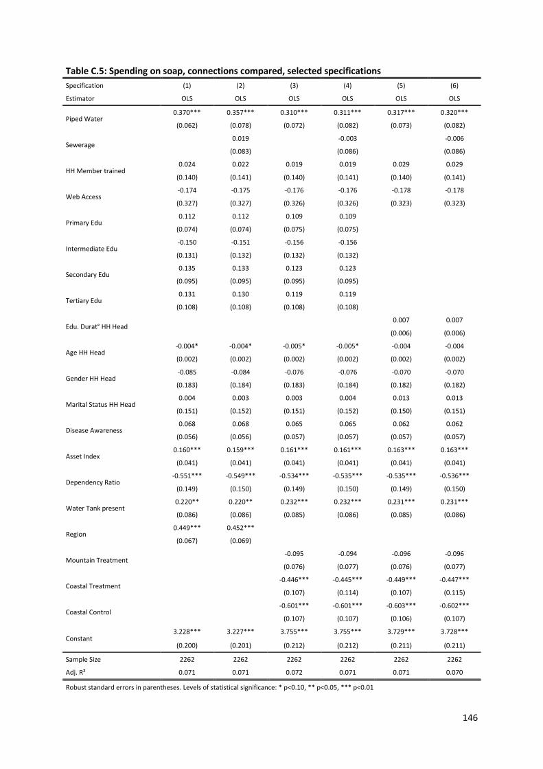
146

Table C.5: Spending on soap, connections compared, selected specifications Specification (1) (2) (3) (4) (5) (6)

Estimator OLS OLS OLS OLS OLS OLS

Piped Water 0.370*** 0.357*** 0.310*** 0.311*** 0.317*** 0.320***

(0.062) (0.078) (0.072) (0.082) (0.073) (0.082)

Sewerage 0.019 -0.003 -0.006

(0.083) (0.086) (0.086)

HH Member trained 0.024 0.022 0.019 0.019 0.029 0.029

(0.140) (0.141) (0.140) (0.141) (0.140) (0.141)

Web Access -0.174 -0.175 -0.176 -0.176 -0.178 -0.178

(0.327) (0.327) (0.326) (0.326) (0.323) (0.323)

Primary Edu 0.112 0.112 0.109 0.109

(0.074) (0.074) (0.075) (0.075)

Intermediate Edu -0.150 -0.151 -0.156 -0.156 (0.131) (0.132) (0.132) (0.132)

Secondary Edu 0.135 0.133 0.123 0.123

(0.095) (0.095) (0.095) (0.095)

Tertiary Edu 0.131 0.130 0.119 0.119

(0.108) (0.108) (0.108) (0.108)

Edu. Durat° HH Head 0.007 0.007

(0.006) (0.006)

Age HH Head -0.004* -0.004* -0.005* -0.005* -0.004 -0.004

(0.002) (0.002) (0.002) (0.002) (0.002) (0.002)

Gender HH Head -0.085 -0.084 -0.076 -0.076 -0.070 -0.070

(0.183) (0.184) (0.183) (0.184) (0.182) (0.182)

Marital Status HH Head 0.004 0.003 0.003 0.004 0.013 0.013

(0.151) (0.152) (0.151) (0.152) (0.150) (0.151)

Disease Awareness 0.068 0.068 0.065 0.065 0.062 0.062

(0.056) (0.056) (0.057) (0.057) (0.057) (0.057)

Asset Index 0.160*** 0.159*** 0.161*** 0.161*** 0.163*** 0.163***

(0.041) (0.041) (0.041) (0.041) (0.041) (0.041)

Dependency Ratio -0.551*** -0.549*** -0.534*** -0.535*** -0.535*** -0.536***

(0.149) (0.150) (0.149) (0.150) (0.149) (0.150)

Water Tank present 0.220** 0.220** 0.232*** 0.232*** 0.231*** 0.231***

(0.086) (0.086) (0.085) (0.086) (0.085) (0.086)

Region 0.449*** 0.452*** (0.067) (0.069)

Mountain Treatment -0.095 -0.094 -0.096 -0.096

(0.076) (0.077) (0.076) (0.077)

Coastal Treatment -0.446*** -0.445*** -0.449*** -0.447***

(0.107) (0.114) (0.107) (0.115)

Coastal Control -0.601*** -0.601*** -0.603*** -0.602***

(0.107) (0.107) (0.106) (0.107)

Constant 3.228*** 3.227*** 3.755*** 3.755*** 3.729*** 3.728***

(0.200) (0.201) (0.212) (0.212) (0.211) (0.211)

Sample Size 2262 2262 2262 2262 2262 2262

Adj. R² 0.071 0.071 0.072 0.071 0.071 0.070

Robust standard errors in parentheses. Levels of statistical significance: * p<0.10, ** p<0.05, *** p<0.01

147

education in combination with the Gender being male has to be calculated136 based on the sum of

the education and interaction term coefficients (-0.816 to -0.885). This corresponds to a remarkable

percentage change of -55.8 to -58.7 per cent. It cannot be entirely clarified why the household head

being male and having completed an intermediate level of education appears more than halving the

spending on soap compared with that of female household heads, ceteris paribus.

A similar picture I find for spending on cleanser when defined broader, as a combination of soap and

detergent. An overview is given in Table C.21 below. Table C.21 to Table C.24 and Table C.29 in

Appendix C.6 are complementary. A few changes arise: exposure to ICT gains in importance with

estimated effects ranging between 25.7 per cent (Landline connection) to doubling (Television Set).

Training comes in with an effect ranging between 42.2 and 54.0%. Symptom Occurrence is higher

correlated (16 to 18%) and more often statistically significant at conventional levels. The coefficient

of Intermediate education is now statistically significant at the ten per cent (in one case at the five

per cent) level in more specifications, while the Interaction Term no longer is. Connection to Piped

Water is significant only occasionally and at the one per cent level, while connection to Improved

Sewerage appears to lose its importance altogether. Presence of a Water Storage Tank and

possession of a Radio broadcasting receiver seem no longer to be influential.

As before, I test for robustness of the results by estimating different specifications. On top of that, I

chose two dependent variables, defining it first narrow (soap only) and then broader (cleanser, i.e.

soap and detergent). Within each of these two cases, the estimations are robust over all

specifications for almost all of the explanatory variables regarding levels of statistical significance,

direction of sign and relative coefficient size. In addition, over different specifications, the absolute

coefficient sizes remain stable. Including alternative measures for education – Duration and Literacy

instead of Level – and of household composition – Number of Children, Elderly or both – does not

change the picture. Comparing the estimated coefficients of the explanatory variables for both

dependent variables shows that they are of similar size and mostly display the same relative order.

The main difference between the narrow and the broader defined models are the entry of Training

experience and the exit of presence of a Water Storage Tank as supposable determinants.

136 Note that for regressing the dependent variable Spending on Soap the OLS estimator is used. Thus the procedure introduced by Ai and Norton (2003); and used, for example, by Dreher et al. (2010) – analysing marginal effects of interaction terms in Probit regressions by means of graphs – does not apply here.

148

Table C.6: Spending on cleanser, connections compared, selected specifications Specification (1) (2) (3) (4) (5) (6)

Estimator OLS OLS OLS OLS OLS OLS

Piped Water 0.284*** 0.233*** 0.141* 0.125 0.149** 0.136

(0.070) (0.082) (0.073) (0.083) (0.074) (0.083)

Sewerage 0.073 0.030 0.025

(0.084) (0.086) (0.086)

HH Member trained 0.440*** 0.433*** 0.430*** 0.427*** 0.438*** 0.436***

(0.104) (0.105) (0.104) (0.105) (0.104) (0.105)

Web Access -0.337 -0.336 -0.335 -0.335 -0.344 -0.344

(0.363) (0.364) (0.362) (0.362) (0.359) (0.359)

Primary Edu 0.048 0.047 0.044 0.044

(0.081) (0.081) (0.081) (0.081)

Intermediate Edu -0.195 -0.201 -0.209 -0.211 (0.148) (0.148) (0.148) (0.149)

Secondary Edu 0.042 0.038 0.024 0.023

(0.102) (0.102) (0.103) (0.103)

Tertiary Edu -0.008 -0.012 -0.027 -0.028 (0.119) (0.119) (0.120) (0.120)

Edu. Durat° HH Head -0.000 -0.000

(0.006) (0.006)

Age HH Head -0.009*** -0.009*** -0.009*** -0.009*** -0.009*** -0.009***

(0.003) (0.003) (0.003) (0.003) (0.003) (0.003)

Gender HH Head -0.060 -0.055 -0.043 -0.041 -0.040 -0.039

(0.190) (0.191) (0.190) (0.191) (0.190) (0.190)

Marital Status HH Head 0.093 0.088 0.088 0.086 0.090 0.089

(0.155) (0.156) (0.155) (0.156) (0.154) (0.155)

Disease Awareness 0.261*** 0.262*** 0.258*** 0.259*** 0.258*** 0.258***

(0.061) (0.061) (0.062) (0.061) (0.062) (0.061)

Asset Index 0.190*** 0.189*** 0.193*** 0.192*** 0.192*** 0.192***

(0.045) (0.045) (0.045) (0.045) (0.045) (0.045)

Dependency Ratio -0.623*** -0.614*** -0.600*** -0.597*** -0.602*** -0.600***

(0.165) (0.166) (0.165) (0.166) (0.166) (0.166)

Water Tank present 0.071 0.069 0.088 0.086 0.085 0.084

(0.092) (0.092) (0.091) (0.092) (0.091) (0.092)

Region 0.506*** 0.517*** (0.071) (0.074)

Mountain Treatment -0.014 -0.017 -0.015 -0.017

(0.073) (0.074) (0.074) (0.075)

Coastal Treatment -0.383*** -0.394*** -0.384*** -0.393***

(0.108) (0.115) (0.109) (0.115)

Coastal Control -0.649*** -0.651*** -0.645*** -0.647***

(0.115) (0.116) (0.115) (0.115)

Constant 4.219*** 4.215*** 4.762*** 4.766*** 4.735*** 4.739***

(0.228) (0.229) (0.240) (0.240) (0.238) (0.238)

Sample Size 1992 1992 1992 1992 1992 1992

Adj. R² 0.077 0.077 0.078 0.078 0.078 0.078

Robust standard errors in parentheses. Levels of statistical significance: * p<0.10, ** p<0.05, *** p<0.01

149

I use 2SLS to control for endogeneity for the dependent variables referring to expenditures for soap

and cleanser. Levels of statistical significance and coefficient signs are mostly consistent with all of

the basic OLS models for most of the explanatory and control variables. The same issues apply as

mentioned above and in Appendix C.4 regarding the exogeneity assumption, so endogeneity – while

I do not assume it to be likely – cannot be ruled out.

Frequency of latrine-cleaning

This section deals with the third alternative proxy of hygiene habits, employed to check for the

robustness of the findings for the dependent variable Probability of Cleanser Use: the frequency,

with which households use to clean their latrines. Descriptive statistics do not show striking

differences between connection groups or topographic regions (see Table C.7).

Table C.7: Mean frequency of latrine-cleaning by location and connection status

Connection Mountain Project N SD

Mountain Control N SD Coastal

Project N SD Coastal

Control N SD

None 7.86 355 3.28 7.77 291 2.64 - - - 7.19 401 3.30

Piped Water 8.12 197 3.57 - - - 7.65 124 2.92 - - -

Sewerage 7.80 268 3.39 - - - 8.60 713 3.28 - - -

N over all connection groups and locations: 2349

Note: no households are connected to piped water or improved sewerage in the control towns. All households in the sample are connected in the coastal project town.

Households tend to report the frequency of cleaning to be daily. Frequency is reported in times per

week, and the modus is seven. This may either reflect a widespread habit to actually conduct

cleaning daily, or the Hawthorne effect mentioned above in the data section.

An overview is given in Table C.8 below. Table C.25 to Table C.28 and Table C.29 in the results

appendix are complementary. The coefficient of determination of the models ranges from three to

five per cent.

The frequency of latrine cleaning is positively correlated with nine explanatory variables or groups of

variables, which are endowed with coefficients statistically significant at conventional levels.

Coefficient size ranges I show in parentheses. Due to the employment of a linear estimator, I can

interpret them straightforward as percentage effects. For instance, a coefficient sized 0.834

corresponds to an increase of frequency of latrine cleaning of about 83 per cent, ceteris paribus.

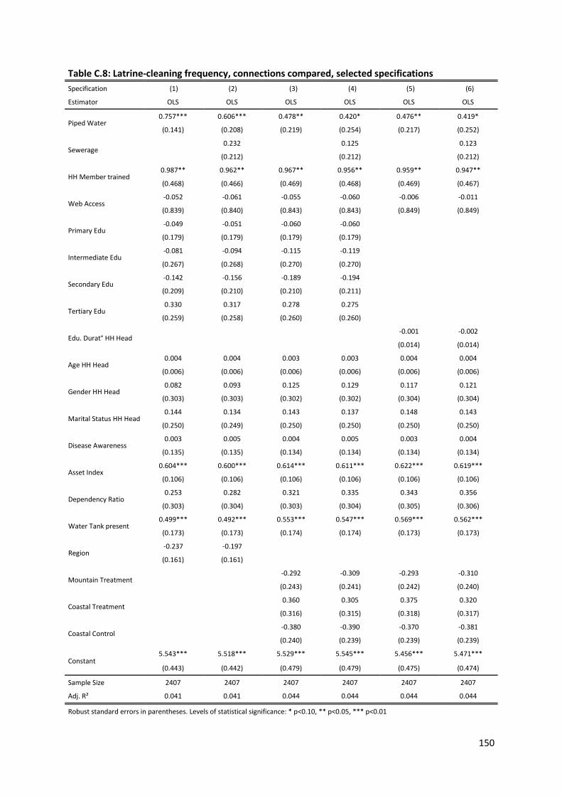
150

Table C.8: Latrine-cleaning frequency, connections compared, selected specifications Specification (1) (2) (3) (4) (5) (6)

Estimator OLS OLS OLS OLS OLS OLS

Piped Water 0.757*** 0.606*** 0.478** 0.420* 0.476** 0.419*

(0.141) (0.208) (0.219) (0.254) (0.217) (0.252)

Sewerage 0.232 0.125 0.123

(0.212) (0.212) (0.212)

HH Member trained 0.987** 0.962** 0.967** 0.956** 0.959** 0.947**

(0.468) (0.466) (0.469) (0.468) (0.469) (0.467)

Web Access -0.052 -0.061 -0.055 -0.060 -0.006 -0.011

(0.839) (0.840) (0.843) (0.843) (0.849) (0.849)

Primary Edu -0.049 -0.051 -0.060 -0.060 (0.179) (0.179) (0.179) (0.179)

Intermediate Edu -0.081 -0.094 -0.115 -0.119 (0.267) (0.268) (0.270) (0.270)

Secondary Edu -0.142 -0.156 -0.189 -0.194 (0.209) (0.210) (0.210) (0.211)

Tertiary Edu 0.330 0.317 0.278 0.275

(0.259) (0.258) (0.260) (0.260)

Edu. Durat° HH Head -0.001 -0.002

(0.014) (0.014)

Age HH Head 0.004 0.004 0.003 0.003 0.004 0.004

(0.006) (0.006) (0.006) (0.006) (0.006) (0.006)

Gender HH Head 0.082 0.093 0.125 0.129 0.117 0.121

(0.303) (0.303) (0.302) (0.302) (0.304) (0.304)

Marital Status HH Head 0.144 0.134 0.143 0.137 0.148 0.143

(0.250) (0.249) (0.250) (0.250) (0.250) (0.250)

Disease Awareness 0.003 0.005 0.004 0.005 0.003 0.004

(0.135) (0.135) (0.134) (0.134) (0.134) (0.134)

Asset Index 0.604*** 0.600*** 0.614*** 0.611*** 0.622*** 0.619***

(0.106) (0.106) (0.106) (0.106) (0.106) (0.106)

Dependency Ratio 0.253 0.282 0.321 0.335 0.343 0.356

(0.303) (0.304) (0.303) (0.304) (0.305) (0.306)

Water Tank present 0.499*** 0.492*** 0.553*** 0.547*** 0.569*** 0.562***

(0.173) (0.173) (0.174) (0.174) (0.173) (0.173)

Region -0.237 -0.197 (0.161) (0.161)

Mountain Treatment -0.292 -0.309 -0.293 -0.310

(0.243) (0.241) (0.242) (0.240)

Coastal Treatment 0.360 0.305 0.375 0.320

(0.316) (0.315) (0.318) (0.317)

Coastal Control -0.380 -0.390 -0.370 -0.381

(0.240) (0.239) (0.239) (0.239)

Constant 5.543*** 5.518*** 5.529*** 5.545*** 5.456*** 5.471***

(0.443) (0.442) (0.479) (0.479) (0.475) (0.474)

Sample Size 2407 2407 2407 2407 2407 2407

Adj. R² 0.041 0.041 0.044 0.044 0.044 0.044

Robust standard errors in parentheses. Levels of statistical significance: * p<0.10, ** p<0.05, *** p<0.01

151

In roughly descending order of estimated coefficient size the covariates positively correlated are

Mean Education Duration of adults in a household (strongly correlated with a coefficient of 1.071 to

1.115, but only when the covariate Dependency Ratio is included in the specification), Training

experience (0.834 to 0.966), and the Dependency Ratio (0.663 to 0.667, only when Mean Education

Duration of adults is included).

The next in line are connection to Piped Water (0.380 to 0.721), wealth reflected by the Asset Index

(0.544 to 0.611, significant at the one per cent level), and location in the Coastal Project town (0.506,

compared to reference category Mountain Control town, significant only in combination with

connection to Piped Water, but not to Improved Sewerage).

Then follow connection to Improved Sewerage (0.581, only in combination with Region), presence of

a Water Storage Tank (0.464 to 0.559, significant at the one per cent level), Tertiary Level of

Education (0.453, compared to reference category no education, only when the covariate Region is

included), and the three alternative measures of household composition (Number of Household

Members with 0.046 to 0.047, Number of Children with 0.055, Number of Children and Elderly with

0.053 to 0.054).

On the other hand, Frequency of Latrine-Cleaning is negatively correlated with Primary (-0.857 to -

0.861) and Secondary Education when the interaction term (Level of Education interacted with

Gender of the household head, itself not significant) is included in the specification. Location in the

Coastal Control town is negatively correlated, likewise (-0.425 to -0.449), though not significant at

conventional levels in all but two specifications. Location in the Mountainous Region is statistically

significant at the ten per cent level in merely one specification, with a coefficient size of -0.299; and

on top is unstable regarding sign.

Obviously beside the point are some of the other covariates. These include Age, Gender and Marital

Status of the household head, Disease Awareness, and location in the Mountain Project town, an

indicator whether any Soap was bought137 within a recall period of 30 days, exposure to ICT and – as

briefly mentioned above – the Interaction Term.

The results I test for robustness following the same scheme as before, i.e. estimating different

specifications. Coefficient signs, sizes and levels of statistical significance are largely consistent.

Because biased (over-)reporting due to a Hawthorne cannot be dismissed, the findings of this

137 This might give a clue about the importance attached by household members to cleanliness.

152

section should not be overrated, though. Nevertheless, they can be put into perspective with the

findings for the antecedent hygiene habit regressands, and contribute to a more complete picture.

2SLS specifications reveal no critical indication of endogeneity issues, but are of limited informative

value due to the concerns regarding exogeneity of the instruments.

In the following, I discuss the patterns of likely determinants of hygiene habits found for the four

dependent variables (probability of Use of Cleanser for hand washing, Spending on Soap and on

Cleanser, Frequency of Latrine-Cleaning) used to proxy those hygiene habits. The advance is

analogical to the structure used above in the discussion of the findings for the dependent variable

Probability of Drinking Water Treatment. First, I recall each of the theories laid down in the

introduction. Then I assess the role of the respective covariate or group of covariates as a –

potentially joint – determinant of the group of four dependent variables, with attention to sign and

rank. Covariates whose correlation coefficients are never statistically significant at least at the ten

per cent level I do not regard to be influential determinants.

Hypothesis 1b (connecting a household to piped water increases its likelihood of displaying hygiene

habits) is consistently supported by the findings for each of the dependent variables. Connection to

Piped Water ranks among the covariates with the most sizable influence, usually between third and

fifth position. Hypothesis 2b (additional connection of a household to Improved Sewerage decreases

its likelihood of displaying hygiene habits, but to a lesser extent than connection to piped water) can

be supported as well. The correlation is positive for three out of four dependent variables, solely

with Spending on Cleanser apparently not being determined by connection to Improved Sewerage.

The covariate ranks lower than connection to Piped Water for all outcomes. Hypothesis 3b (those

households in which at least one member participated in any type of hygiene Training in the past

have a higher likelihood of displaying hygiene habits) is distinctly reinforced, with coefficients

ranking between first and fifth position. Interestingly, Training experience appears to be the most

important covariate for the outcome Spending on Cleanser including laundry detergent, while it

seems to be irrelevant for Spending on Soap. Hypothesis 4b (those households with exposure to

information and communication technology have a higher likelihood of displaying hygiene habits) is

consistently supported, with the exception of the outcome Frequency of Latrine-Cleaning. For the

latter, the coefficients never reach the ten per cent level of statistical significance. Please note that

there is, in contrast to expectation, no evidence that access to the World Wide Web is a driver.

Instead, those ICT measures that indicate possession of objects (Television Set, Personal Computer,

Satellite Dish, Radio broadcasting receiver and Mobile Phone) make the impression to be. This gives

room for doubt if the correlation does indeed map the influence of increased availability of

153

information, or rather depicts the wealth of the household. On the other hand, the correlation of

connection to a phone Landline with the outcome variables softens this concern slightly, as I believe

such a connection to be far less costly than purchase of electronic goods. Another source of

reassurance is the fact that the Asset Index is used to control for wealth.

Hypothesis 5b (the more educated the head of the household is, the higher is the likelihood of the

household members displaying hygiene habits) can neither be supported nor invalidated. Empirical

evidence is mixed. It indicates a positive relationship of Tertiary (for the Use of Cleanser also of

Secondary) Education on Use of Cleanser for hand washing on the one hand, and on Frequency of

Latrine-Cleaning on the other. However, regarding the expenditure outcomes, no effect is revealed

by the analysis, except for Intermediate education – the coefficients of which are negatively

correlated with the outcomes.

The evidence regarding the control variables covering household composition is mixed. While the

probability of Use of Cleanser and the Spending on Soap seem to be negatively and – with the

coefficient in most specifications being the second largest – strongly influenced, the contrary

appears to be the case for Spending on Cleanser and Latrine-Cleaning Frequency. Female headship

does not seem to play an influential role. The age of the household head is also not fostering hygiene

habits. For two of the outcomes, namely Use of Cleanser for hand washing and Frequency of Latrine-

Cleaning, the coefficients never reach the ten per cent level of statistical significance. For both

expenditure outcomes, a negative correlation – statistically significant at conventional levels up to

the one per cent level – is estimated for most specifications. This is in line with my expectation of

younger household heads being more prone to pursue hygiene habits, and contradicts the previous

literature. Considering that income tends to increase with Age, the relationship between young age

and spending might indeed be understated here, if income is not fully controlled for by the asset

index. This latter control variable is consistently positively correlated with all dependent variables

proxying hygiene habits. The coefficient usually ranks between sixth and ninth position in terms of

relative size. At least one household member having suffered from water-related diseases in the

recent past (i.e., Illness History) is positively correlated with the likelihood of displaying hygiene

habits. Likewise, the covariate Symptom Occurrence is consistently positively correlated with the

outcome variables.

154

C.6 Estimation results

Table C.9: Probability of drinking water treatment, piped water, ICT covariates Specification (1) (2) (3) (4) (5) Estimator Probit Probit Probit Probit Probit

Piped Water 0.055*** 0.053*** 0.054*** 0.053*** 0.052*** (0.012) (0.012) (0.012) (0.012) (0.012)

Age HH Head -0.000 -0.000 -0.000 -0.000 -0.000 (0.000) (0.000) (0.000) (0.000) (0.000)

Gender HH Head -0.045* -0.044* -0.044* -0.050** -0.044* (0.024) (0.024) (0.024) (0.024) (0.024)

Marital Status HH Head 0.013 0.012 0.013 0.011 0.012 (0.021) (0.021) (0.021) (0.020) (0.020)

Disease Awareness 0.007 0.006 0.007 0.005 0.005 (0.011) (0.011) (0.011) (0.011) (0.011)

HH Member trained 0.104*** 0.104*** 0.102*** 0.102*** 0.106*** (0.020) (0.020) (0.020) (0.020) (0.020)

Asset Index 0.040*** 0.038*** 0.038*** 0.034*** 0.036*** (0.007) (0.007) (0.008) (0.008) (0.007)

Dependency Ratio 0.000 0.000 0.005 0.005 0.006 (0.028) (0.028) (0.027) (0.028) (0.028)

Region 0.153*** 0.153*** 0.146*** 0.149*** 0.152*** (0.016) (0.016) (0.016) (0.016) (0.016)

Water Tank present -0.021 -0.022 -0.022 -0.021 -0.021 (0.019) (0.019) (0.019) (0.019) (0.019)

TV present 0.009 (0.019)

Sat. Dish present 0.019

(0.013)

Radio present 0.025**

(0.011)

GSM present 0.032**

(0.014)

Landline Connection 0.028**

(0.012)

Primary Edu 0.045*** 0.044*** 0.044*** 0.045*** 0.044*** (0.014) (0.014) (0.014) (0.014) (0.014)

Intermediate Edu 0.011 0.009 0.009 0.012 0.010 (0.023) (0.023) (0.023) (0.023) (0.023)

Secondary Edu 0.045** 0.043** 0.043** 0.044** 0.042** (0.018) (0.018) (0.018) (0.018) (0.018)

Tertiary Edu 0.046** 0.044** 0.042** 0.044** 0.043** (0.021) (0.021) (0.020) (0.020) (0.020)

Sample Size 2459 2459 2459 2459 2459 Pseudo R² 0.173 0.174 0.176 0.176 0.176 Average marginal effects displayed. Robust standard errors in parentheses. Levels of statistical significance: * p<0.10, ** p<0.05, *** p<0.01

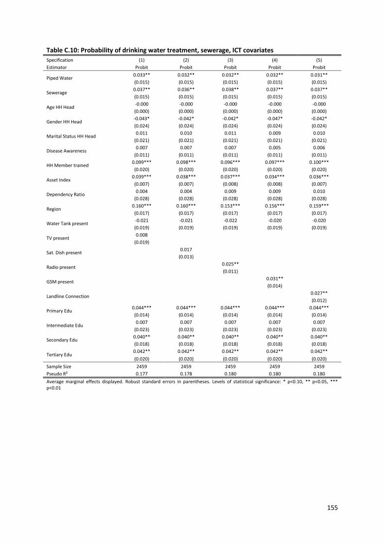
155

Table C.10: Probability of drinking water treatment, sewerage, ICT covariates Specification (1) (2) (3) (4) (5) Estimator Probit Probit Probit Probit Probit

Piped Water 0.033** 0.032** 0.032** 0.032** 0.031** (0.015) (0.015) (0.015) (0.015) (0.015)

Sewerage 0.037** 0.036** 0.038** 0.037** 0.037** (0.015) (0.015) (0.015) (0.015) (0.015)

Age HH Head -0.000 -0.000 -0.000 -0.000 -0.000 (0.000) (0.000) (0.000) (0.000) (0.000)

Gender HH Head -0.043* -0.042* -0.042* -0.047* -0.042* (0.024) (0.024) (0.024) (0.024) (0.024)

Marital Status HH Head 0.011 0.010 0.011 0.009 0.010 (0.021) (0.021) (0.021) (0.021) (0.021)

Disease Awareness 0.007 0.007 0.007 0.005 0.006 (0.011) (0.011) (0.011) (0.011) (0.011)

HH Member trained 0.099*** 0.098*** 0.096*** 0.097*** 0.100*** (0.020) (0.020) (0.020) (0.020) (0.020)

Asset Index 0.039*** 0.038*** 0.037*** 0.034*** 0.036*** (0.007) (0.007) (0.008) (0.008) (0.007)

Dependency Ratio 0.004 0.004 0.009 0.009 0.010 (0.028) (0.028) (0.028) (0.028) (0.028)

Region 0.160*** 0.160*** 0.153*** 0.156*** 0.159*** (0.017) (0.017) (0.017) (0.017) (0.017)

Water Tank present -0.021 -0.021 -0.022 -0.020 -0.020 (0.019) (0.019) (0.019) (0.019) (0.019)

TV present 0.008 (0.019)

Sat. Dish present 0.017

(0.013)

Radio present 0.025**

(0.011)

GSM present 0.031**

(0.014)

Landline Connection 0.027**

(0.012)

Primary Edu 0.044*** 0.044*** 0.044*** 0.044*** 0.044*** (0.014) (0.014) (0.014) (0.014) (0.014)

Intermediate Edu 0.007 0.007 0.007 0.007 0.007 (0.023) (0.023) (0.023) (0.023) (0.023)

Secondary Edu 0.040** 0.040** 0.040** 0.040** 0.040** (0.018) (0.018) (0.018) (0.018) (0.018)

Tertiary Edu 0.042** 0.042** 0.042** 0.042** 0.042** (0.020) (0.020) (0.020) (0.020) (0.020)

Sample Size 2459 2459 2459 2459 2459 Pseudo R² 0.177 0.178 0.180 0.180 0.180 Average marginal effects displayed. Robust standard errors in parentheses. Levels of statistical significance: * p<0.10, ** p<0.05, *** p<0.01

156

Table C.11: Probability of drinking water treatment, piped water, other specifications & estimators Specification (1) (2) (3) (4) (5) (6) Estimator Probit Probit IV-Probit SUR BP 2SLS 2SPrB

Piped Water 0.061*** 0.060*** 0.966*** 0.054*** 0.525*** 0.092

(0.013) (0.014) (0.286) (0.017) (0.172) (0.694)

Age HH Head -0.000 -0.001* -0.002 -0.000 -0.002* 0.000 (0.000) (0.000) (0.003) (0.000) (0.001) (0.005)

Gender HH Head -0.034 -0.022 -0.325* -0.020* -0.021 -0.054* (0.023) (0.023) (0.175) (0.010) (0.031) (0.207)

Marital Status HH Head 0.007 0.013 0.138 0.005 0.022 0.016 (0.020) (0.020) (0.151) (0.008) (0.027) (0.174)

Disease Awareness 0.005 0.003 0.082 0.002 0.025 0.009 (0.011) (0.011) (0.080) (0.004) (0.016) (0.092)

Symptom Occurrence 0.064 0.004 -0.006 0.008

(0.084) (0.005) (0.017) (0.014)

HH Member trained 0.107*** 0.103*** 0.694*** 0.042*** 0.118*** 0.116*** (0.021) (0.021) (0.164) (0.012) (0.040) (0.188)

Asset Index 0.039*** 0.037*** 0.281*** 0.016*** 0.035*** 0.038*** (0.007) (0.007) (0.053) (0.004) (0.011) (0.057)

Dependency Ratio -0.003 0.030 -0.007 -0.004 0.045 -0.004 (0.027) (0.029) (0.205) (0.011) (0.036) (0.242)

Mountain Treatment 0.035** 0.035** 0.005 0.014** -0.115 0.031 (0.016) (0.016) (0.178) (0.007) (0.073) (0.305)

Coastal Treatment -0.146*** -0.153*** -1.520*** -0.062*** -0.508*** -0.192** (0.024) (0.024) (0.273) (0.014) (0.142) (0.571)

Coastal Control -0.072*** -0.073*** -0.492*** -0.030*** (0.024) (0.024) (0.175) (0.011)

Water Tank present -0.025 -0.028 -0.221 -0.010 -0.058*** -0.036 (0.018) (0.018) (0.135) (0.008) (0.018) (0.172)

TV and/or PC present 0.009

(0.183)

Web Access 0.072** 0.077** 0.470* 0.030** 0.107* (0.032) (0.033) (0.243) (0.015) (0.063)

Edu. Durat° HH Head -0.001

(0.002)

Literacy HH Head 0.034** (0.014)

Mean Edu. Durat° Adults 0.095***

(0.030)

Primary Edu 0.283*** 0.018***

0.046**

(0.110) (0.006)

(0.129)

Intermediate Edu 0.062 0.004

0.009

(0.193) (0.009)

(0.224)

Secondary Edu 0.276** 0.020**

0.057**

(0.132) (0.008)

(0.180)

Tertiary Edu 0.242 0.020**

0.058**

(0.150) (0.009)

(0.192)

Sample Size 2459 2464 2393 2459 2029 2029 Pseudo R² 0.180 0.185 0.157 Average marginal effects displayed for non-linear models. Robust standard errors in parentheses; bootstrapped for 2SPrB. Levels of statistical significance: * p<0.10, ** p<0.05, *** p<0.01

157

Table C.12: Probability of drinking water treatment, sewerage, other specifications & estimators Specification (1) (2) (3) (4) (5) (6) Estimator Probit Probit IV-Probit SUR BP 2SLS 2SPrB

Piped Water 0.043*** 0.042*** 0.776* 0.044** 0.251*** -0.003 (0.015) (0.015) (0.464) (0.019) (0.077) (0.755)

Sewerage 0.043*** 0.041*** 0.096 0.017** -0.019 0.072 (0.015) (0.016) (0.240) (0.007) (0.028) (0.420)

Age HH Head -0.000 -0.001* -0.002 -0.000 -0.000 0.000 (0.000) (0.000) (0.004) (0.000) (0.001) (0.005)

Gender HH Head -0.033 -0.021 -0.336* -0.019* -0.032 -0.053* (0.023) (0.023) (0.177) (0.011) (0.025) (0.210)

Marital Status HH Head 0.007 0.013 0.137 0.004 0.018 0.010 (0.020) (0.020) (0.153) (0.009) (0.022) (0.183)

Disease Awareness 0.006 0.005 0.076 0.003 0.012 0.006 (0.011) (0.011) (0.080) (0.004) (0.013) (0.089)

Symptom Occurrence 0.063 0.004 0.003 0.011

(0.086) (0.005) (0.015) (0.093)

HH Member trained 0.104*** 0.099*** 0.704*** 0.041*** 0.149*** 0.115*** (0.021) (0.021) (0.165) (0.012) (0.039) (0.169)

Asset Index 0.040*** 0.038*** 0.283*** 0.015*** 0.039*** 0.037*** (0.007) (0.007) (0.053) (0.004) (0.010) (0.056)

Dependency Ratio 0.001 0.033 -0.018 -0.002 0.008 -0.009 (0.027) (0.029) (0.207) (0.011) (0.030) (0.230)

Mountain Treatment 0.026 0.026 0.044 0.011 0.002 0.041 (0.017) (0.017) (0.183) (0.007) (0.030) (0.214)

Coastal Treatment -0.166*** -0.170*** -1.464*** -0.071*** -0.273*** -0.175*** (0.025) (0.025) (0.260) (0.017) (0.050) (0.302)

Coastal Control -0.075*** -0.076*** -0.514*** -0.032*** (0.024) (0.024) (0.184) (0.012)

Water Tank present -0.026 -0.028 -0.210 -0.010 -0.039*** -0.030 (0.018) (0.018) (0.135) (0.008) (0.015) (0.159)

TV and/or PC present 0.018

(0.176)

Web Access 0.470* 0.028* 0.140**

(0.251) (0.015) (0.064)

Edu. Durat° HH Head 0.002

(0.001)

Literacy HH Head 0.034** (0.014) Mean Edu. Durat°

Adults 0.090***

(0.030)

Primary Edu 0.296*** 0.018***

0.050***

(0.112) (0.007)

(0.133)

Intermediate Edu 0.063 0.004

0.009

(0.195) (0.009)

(0.227)

Secondary Edu 0.304** 0.020**

0.067***

(0.135) (0.008)

(0.169)

Tertiary Edu 0.272* 0.020**

0.068**

(0.154) (0.009)

(0.190)

Sample Size 2459 2463 2393 2459 2029 2029 Pseudo R² 0.183 0.185

0.172

Average marginal effects displayed for non-linear models. Robust standard errors in parentheses; bootstrapped for 2SPrB . Levels of statistical significance: * p<0.10, ** p<0.05, *** p<0.01

158

Table C.13: Probability of cleanser use, piped water, ICT covariates Specification (1) (2) (3) (4) (5) Estimator Probit Probit Probit Probit Probit

Piped Water 0.121*** 0.118*** 0.122*** 0.120*** 0.116*** (0.024) (0.024) (0.024) (0.024) (0.024)

Age HH Head 0.000 0.000 0.000 0.001 0.000 (0.001) (0.001) (0.001) (0.001) (0.001)

Gender HH Head -0.001 -0.001 0.001 -0.006 -0.000 (0.046) (0.046) (0.046) (0.046) (0.046)

Marital Status HH Head -0.001 -0.000 0.000 -0.003 -0.002 (0.040) (0.040) (0.040) (0.040) (0.040)

Disease Awareness 0.040** 0.038** 0.041** 0.038** 0.040** (0.017) (0.017) (0.017) (0.017) (0.017)

HH Member trained 0.091* 0.092* 0.089* 0.090* 0.098** (0.050) (0.050) (0.050) (0.050) (0.049)

Asset Index 0.040*** 0.038*** 0.039*** 0.031** 0.032** (0.013) (0.013) (0.013) (0.014) (0.013)

Dependency Ratio -0.195*** -0.197*** -0.190*** -0.189*** -0.183*** (0.041) (0.041) (0.041) (0.040) (0.040)

Mountain Treatment 0.003 0.002 -0.001 -0.001 0.001 (0.027) (0.027) (0.027) (0.027) (0.027)

Coastal Treatment 0.157*** 0.153*** 0.163*** 0.161*** 0.156*** (0.035) (0.035) (0.035) (0.035) (0.035)

Coastal Control 0.224*** 0.219*** 0.223*** 0.220*** 0.219*** (0.031) (0.031) (0.031) (0.031) (0.031)

Water Tank present 0.008 0.009 0.010 0.013 0.009 (0.024) (0.024) (0.024) (0.024) (0.024)

TV present 0.043* (0.025)

Sat. Dish present 0.048**

(0.019)

Radio present 0.044**

(0.019)

GSM present 0.048**

(0.020)

Landline Connection 0.087***

(0.022)

Primary Edu -0.006 -0.008 -0.006 -0.005 -0.007 (0.024) (0.024) (0.024) (0.024) (0.024)

Intermediate Edu 0.052 0.051 0.053 0.054 0.050 (0.039) (0.039) (0.039) (0.038) (0.038)

Secondary Edu 0.082*** 0.079*** 0.082*** 0.081*** 0.077*** (0.028) (0.029) (0.028) (0.028) (0.028)

Tertiary Edu 0.098*** 0.094*** 0.096*** 0.096*** 0.091*** (0.031) (0.032) (0.032) (0.032) (0.032)

Sample Size 2466 2466 2466 2466 2466 Pseudo R² 0.090 0.091 0.090 0.090 0.094 Average marginal effects displayed. Robust standard errors in parentheses. Levels of statistical significance: * p<0.10, ** p<0.05, *** p<0.01

159

Table C.14: Probability of cleanser use, sewerage, ICT covariates Specification (1) (2) (3) (4) (5) Estimator Probit Probit Probit Probit Probit

Piped Water 0.099*** 0.096*** 0.100*** 0.098*** 0.095*** (0.027) (0.027) (0.027) (0.027) (0.027)

Sewerage 0.048* 0.047* 0.049* 0.049* 0.047* (0.027) (0.027) (0.027) (0.027) (0.027)

Age HH Head 0.000 0.000 0.000 0.001 0.000 (0.001) (0.001) (0.001) (0.001) (0.001)

Gender HH Head 0.001 0.001 0.002 -0.005 0.001 (0.046) (0.046) (0.046) (0.046) (0.046)

Marital Status HH Head -0.004 -0.002 -0.002 -0.005 -0.005 (0.040) (0.040) (0.040) (0.040) (0.040)

Disease Awareness 0.041** 0.038** 0.042** 0.038** 0.040** (0.017) (0.017) (0.017) (0.017) (0.017)

HH Member trained 0.084* 0.086* 0.083* 0.084* 0.091* (0.050) (0.050) (0.050) (0.050) (0.049)

Asset Index 0.039*** 0.037*** 0.038*** 0.030** 0.031** (0.013) (0.013) (0.013) (0.014) (0.013)

Dependency Ratio -0.189*** -0.191*** -0.184*** -0.183*** -0.178*** (0.041) (0.040) (0.041) (0.040) (0.040)

Mountain Treatment -0.004 -0.004 -0.007 -0.007 -0.005 (0.027) (0.027) (0.027) (0.027) (0.027)

Coastal Treatment 0.137*** 0.134*** 0.142*** 0.140*** 0.137*** (0.037) (0.037) (0.037) (0.037) (0.037)

Coastal Control 0.219*** 0.215*** 0.219*** 0.216*** 0.215*** (0.031) (0.031) (0.031) (0.031) (0.031)

Water Tank present 0.006 0.007 0.007 0.010 0.007 (0.024) (0.024) (0.024) (0.024) (0.024)

TV present 0.042* (0.025)

Sat. Dish present 0.047**

(0.019)

Radio present 0.043**

(0.019)

GSM present 0.048**

(0.020)

Landline Connection 0.086***

(0.022)

Primary Edu -0.007 -0.008 -0.006 -0.006 -0.008 (0.024) (0.024) (0.024) (0.024) (0.024)

Intermediate Edu 0.050 0.049 0.051 0.052 0.048 (0.039) (0.039) (0.039) (0.038) (0.038)

Secondary Edu 0.080*** 0.077*** 0.080*** 0.079*** 0.075*** (0.029) (0.029) (0.028) (0.028) (0.028)

Tertiary Edu 0.097*** 0.093*** 0.094*** 0.094*** 0.089*** (0.031) (0.032) (0.032) (0.032) (0.032)

Sample Size 2466 2466 2466 2466 2466 Pseudo R² 0.091 0.092 0.091 0.092 0.095 Average marginal effects displayed. Robust standard errors in parentheses. Levels of statistical significance: * p<0.10, ** p<0.05, *** p<0.01

160

Table C.15: Probability of cleanser use, piped water, other specifications & estimators Specification (1) (2) (3) (4) (5) (6) (7) (8) (9) Estimator Probit Probit Probit Probit Probit IV-Probit SUR BP 2SLS 2SPrB

Piped Water 0.116*** 0.124*** 0.123*** 0.130*** 0.125*** 0.877*** 0.218*** 0.292 -0.082 (0.024) (0.024) (0.024) (0.024) (0.024) (0.203) (0.045) (0.193) (0.557)

Age HH Head 0.001 -0.000 -0.001 0.001 0.000 0.000 0.000 0.001 0.001

(0.001) (0.001) (0.001) (0.001) (0.001) (0.002) (0.000) (0.001) (0.003)

Gender HH Head -0.015 0.019 0.033 0.028 0.016 0.012 -0.002 0.018 0.018 (0.046) (0.046) (0.045) (0.045) (0.046) (0.148) (0.022) (0.046) (0.174)

Marital Status HH Head -0.003 -0.019 -0.013 -0.021 -0.003 0.011 0.002 -0.048 -0.063 (0.040) (0.041) (0.040) (0.039) (0.040) (0.130) (0.019) (0.039) (0.153)

Disease Awareness 0.037** 0.041** 0.040** 0.040** 0.040** 0.129** 0.021** 0.067*** 0.050** (0.017) (0.018) (0.017) (0.017) (0.017) (0.057) (0.009) (0.021) (0.070)

Symptom Occurrence 0.052 0.013 0.034 0.045**

(0.062) (0.010) (0.022) (0.072)

HH Member trained 0.087* 0.093* 0.091* 0.100** 0.098** 0.249 0.043* 0.043 0.115** (0.049) (0.050) (0.050) (0.050) (0.050) (0.166) (0.026) (0.038) (0.180)

Asset Index 0.037*** 0.044*** 0.043*** 0.048*** 0.047*** 0.130*** 0.023*** 0.039*** 0.045*** (0.013) (0.013) (0.013) (0.013) (0.013) (0.042) (0.007) (0.013) (0.048)

Dependency Ratio -0.202*** -0.179*** -0.151***

-0.596*** -0.097*** -0.205*** -0.248***

(0.041) (0.040) (0.042)

(0.135) (0.027) (0.050) (0.170)

# of HH Members -0.007***

(0.002)

# of Children -0.019***

(0.004)

Mountain Treatment 0.004 0.003 0.003 -0.002 -0.001 -0.176 0.001 -0.057 0.078

(0.027) (0.028) (0.027) (0.027) (0.027) (0.117) (0.013) (0.084) (0.239)

Coastal Treatment 0.155*** 0.175*** 0.170*** 0.161*** 0.155*** 0.098 0.073*** 0.023 0.329** (0.035) (0.035) (0.035) (0.036) (0.036) (0.198) (0.021) (0.157) (0.472)

Coastal Control 0.224*** 0.233*** 0.231*** 0.225*** 0.222*** 0.742*** 0.099***

(0.031) (0.031) (0.031) (0.031) (0.031) (0.103) (0.026)

Water Tank present 0.006 0.015 0.014 0.017 0.014 0.022 0.008 0.002 0.039

(0.024) (0.024) (0.024) (0.024) (0.024) (0.078) (0.012) (0.027) (0.106)

TV present 0.041* 0.044* 0.040 0.050** 0.048*

(0.025) (0.025) (0.025) (0.025) (0.024)

TV and/or PC present 0.043

(0.113)

Web Access 0.032 0.041 0.044 0.030 0.032 0.045 0.016 -0.008

(0.082) (0.082) (0.082) (0.082) (0.083) (0.268) (0.041) (0.071)

Edu. Durat° HH Head 0.009***

0.008***

(0.002)

(0.003)

Literacy HH Head 0.045**

(0.021)

Mean Edu. Durat° Adults 0.091*

(0.051)

Primary Edu -0.008 -0.009 -0.023 -0.003

0.033

(0.024) (0.024) (0.074) (0.011)

(0.092)

Intermediate Edu 0.041 0.043 0.168 0.026

0.071

(0.039) (0.039) (0.127) (0.020)

(0.145)

Secondary Edu 0.065** 0.070** 0.224** 0.040**

0.134***

(0.029) (0.028) (0.098) (0.016)

(0.134)

Tertiary Edu 0.079** 0.084*** 0.274** 0.050***

0.137***

(0.032) (0.031) (0.111) (0.018)

(0.146)

Sample Size 2466 2466 2471 2466 2466 2400 2466 2037 2037 Adj. R²

0.105

Pseudo R² 0.093 0.086 0.085 0.085 0.089

0.097

Average marginal effects displayed for non-linear models. Robust standard errors in parentheses; bootstrapped for 2SPrB. Levels of statistical significance: * p<0.10, ** p<0.05, *** p<0.01

161

Table C.16: Probability of cleanser use, sewerage, other specifications & estimators Specification (1) (2) (3) (4) (5) (6) (7) (8) (9) Estimator Probit Probit Probit Probit Probit IV-Probit SUR BP 2SLS 2SPrB

Piped Water 0.094*** 0.100*** 0.100*** 0.105*** 0.103*** 0.911*** 0.203*** 0.227** 0.047

(0.027) (0.027) (0.027) (0.027) (0.027) (0.329) (0.050) (0.111) (0.338)

Sewerage 0.047* 0.053* 0.051* 0.054** 0.048* -0.055 0.024* 0.002 0.070 (0.027) (0.027) (0.027) (0.027) (0.027) (0.163) (0.014) (0.050) (0.162)

Age HH Head 0.001 -0.000 -0.001 0.001 0.000 0.000 0.000 0.001 0.001

(0.001) (0.001) (0.001) (0.001) (0.001) (0.002) (0.000) (0.001) (0.003)

Gender HH Head -0.014 0.020 0.033 0.029 0.017 0.009 -0.001 0.016 0.026 (0.046) (0.046) (0.045) (0.045) (0.045) (0.147) (0.023) (0.045) (0.167)

Marital Status HH Head

-0.005 -0.020 -0.015 -0.022 -0.005 0.013 0.001 -0.050 -0.061 (0.040) (0.041) (0.040) (0.039) (0.040) (0.131) (0.020) (0.039) (0.147)

Disease Awareness 0.038** 0.042** 0.041** 0.040** 0.040** 0.129** 0.021** 0.064*** 0.058*** (0.017) (0.017) (0.017) (0.017) (0.017) (0.057) (0.009) (0.020) (0.064)

Symptom Occurrence

0.050 0.013 0.037* 0.041*

(0.063) (0.010) (0.021) (0.069)

HH Member trained 0.081 0.086* 0.082 0.092* 0.091* 0.247 0.040 0.050 0.082

(0.049) (0.050) (0.051) (0.050) (0.050) (0.165) (0.026) (0.035) (0.167)

Asset Index 0.036*** 0.043*** 0.042*** 0.047*** 0.046*** 0.131*** 0.022*** 0.040*** 0.042*** (0.013) (0.013) (0.013) (0.013) (0.013) (0.042) (0.007) (0.013) (0.047)

Dependency Ratio

-0.197*** -0.174*** -0.148*** -0.599*** -0.096*** -0.213*** -0 217*** (0.041) (0.040) (0.042) (0.135) (0.026) (0.045) (0.153)

# of HH Members -0.007***

(0.002)

# of Children -0.018*** (0.004)

Mountain Treatment

-0.002 -0.003 -0.003 -0.009 -0.006 -0.171 -0.002 -0.032 0.005 (0.027) (0.028) (0.027) (0.028) (0.027) (0.124) (0.013) (0.045) (0.123)

Coastal Treatment 0.135*** 0.153*** 0.149*** 0.138*** 0.135*** 0.117 0.064*** 0.073 0.165***

(0.037) (0.037) (0.037) (0.037) (0.037) (0.203) (0.021) (0.065) (0.203)

Coastal Control 0.220*** 0.228*** 0.226*** 0.219*** 0.217*** 0.744*** 0.099*** (0.031) (0.031) (0.031) (0.031) (0.031) (0.106) (0.025)

Water Tank present 0.004 0.012 0.012 0.014 0.012 0.024 0.007 0.006 0.022

(0.024) (0.024) (0.024) (0.024) (0.024) (0.078) (0.012) (0.025) (0.097)

TV present 0.040 0.043* 0.039 0.049** 0.046*

(0.025) (0.025) (0.025) (0.025) (0.024) TV and/or PC present

0.025

(0.102)

Web Access 0.028 0.036 0.040 0.026 0.028 0.043 0.014 -0.001

(0.082) (0.081) (0.082) (0.082) (0.082) (0.268) (0.041) (0.069) Edu. Durat° HH Head

0.009*** 0.009*** (0.002) (0.002)

Literacy HH Head 0.043** (0.021)

Mean Edu. Durat° Adults

0.083 (0.051)

Primary Edu -0.008 -0.009 -0.024 -0.004 0.021

(0.024) (0.024) (0.075) (0.011) (0.084)

Intermediate Edu 0.039 0.041 0.168 0.025 0.063

(0.039) (0.039) (0.127) (0.020) (0.140)

Secondary Edu 0.064** 0.068** 0.225** 0.040** 0.108**

(0.029) (0.028) (0.099) (0.016) (0.111)

Tertiary Edu 0.078** 0.083*** 0.273** 0.050*** 0.113**

(0.032) (0.031) (0.111) (0.018) (0.125)

Sample Size 2466 2466 2470 2466 2466 2400 2466 2037 2037

Adj. R² 0.114 Pseudo R² 0.094 0.087 0.086 0.086 0.090 0.102

Average marginal effects displayed for non-linear models. Robust standard errors in parentheses; bootstrapped for 2SPrB. Levels of statistical significance: * p<0.10, ** p<0.05, *** p<0.01

162

Table C.17: Spending on soap, piped water, ICT covariates Specification (1) (2) (3) (4) (5) Estimator OLS OLS OLS OLS OLS

Piped Water 0.262*** 0.224*** 0.296*** 0.264*** 0.285*** (0.073) (0.073) (0.073) (0.074) (0.073)

Age HH Head -0.005** -0.005** -0.005* -0.004* -0.006** (0.002) (0.002) (0.002) (0.002) (0.002)

Gender HH Head -0.113 -0.078 -0.072 -0.123 -0.070 (0.180) (0.182) (0.182) (0.184) (0.182)

Marital Status HH Head 0.008 0.003 0.001 -0.019 -0.009 (0.148) (0.150) (0.150) (0.153) (0.151)

Disease Awareness 0.037 0.030 0.061 0.038 0.059 (0.055) (0.056) (0.056) (0.056) (0.056)

HH Member trained -0.043 -0.023 -0.007 -0.033 0.013 (0.138) (0.141) (0.138) (0.136) (0.136)

Asset Index 0.094** 0.102** 0.139*** 0.049 0.127*** (0.040) (0.041) (0.041) (0.045) (0.042)

Dependency Ratio -0.515*** -0.534*** -0.501*** -0.479*** -0.490*** (0.145) (0.147) (0.149) (0.148) (0.151)

Mountain Treatment -0.075 -0.079 -0.109 -0.101 -0.096 (0.077) (0.078) (0.076) (0.077) (0.076)

Coastal Treatment -0.394*** -0.434*** -0.404*** -0.372*** -0.440*** (0.106) (0.107) (0.107) (0.107) (0.106)

Coastal Control -0.396*** -0.530*** -0.556*** -0.532*** -0.581*** (0.101) (0.104) (0.107) (0.104) (0.106)

Water Tank present 0.191** 0.211** 0.224*** 0.246*** 0.223*** (0.083) (0.083) (0.085) (0.084) (0.085)

TV present 0.819*** (0.103)

Sat. Dish present 0.549***

(0.074)

Radio present 0.202***

(0.059)

GSM present 0.430***

(0.072)

Landline Connection 0.231***

(0.065)

Primary Edu 0.085 0.069 0.106 0.098 0.100 (0.073) (0.074) (0.074) (0.074) (0.074)

Intermediate Edu -0.199 -0.205 -0.166 -0.166 -0.167 (0.129) (0.129) (0.131) (0.130) (0.132)

Secondary Edu 0.091 0.068 0.118 0.098 0.103 (0.094) (0.095) (0.095) (0.094) (0.095)

Tertiary Edu 0.117 0.074 0.099 0.075 0.087 (0.104) (0.106) (0.108) (0.107) (0.109)

Constant 3.287*** 3.615*** 3.707*** 3.741*** 3.827*** (0.216) (0.209) (0.212) (0.210) (0.212) Sample Size 2.262 2.262 2.262 2.262 2.262 Adj. R² 0.113 0.100 0.076 0.089 0.076

Robust standard errors in parentheses. Levels of statistical significance: * p<0.10, ** p<0.05, *** p<0.01

163

Table C.18: Spending on soap, sewerage, ICT covariates Specification (1) (2) (3) (4) (5) Estimator OLS OLS OLS OLS OLS

Piped Water 0.277*** 0.239*** 0.297*** 0.268*** 0.290*** (0.083) (0.082) (0.082) (0.083) (0.082)

Sewerage -0.031 -0.030 -0.002 -0.009 -0.010 (0.087) (0.087) (0.086) (0.086) (0.086)

Age HH Head -0.005** -0.005** -0.005* -0.004* -0.006** (0.002) (0.002) (0.002) (0.002) (0.002)

Gender HH Head -0.114 -0.079 -0.073 -0.123 -0.070 (0.181) (0.183) (0.183) (0.184) (0.183)

Marital Status HH Head 0.009 0.005 0.001 -0.019 -0.009 (0.148) (0.150) (0.150) (0.154) (0.151)

Disease Awareness 0.037 0.029 0.061 0.038 0.059 (0.055) (0.056) (0.056) (0.056) (0.056)

HH Member trained -0.040 -0.020 -0.007 -0.032 0.014 (0.139) (0.142) (0.139) (0.137) (0.137)

Asset Index 0.094** 0.103** 0.139*** 0.049 0.127*** (0.040) (0.041) (0.041) (0.045) (0.042)

Dependency Ratio -0.519*** -0.537*** -0.501*** -0.480*** -0.491*** (0.146) (0.148) (0.150) (0.149) (0.151)

Mountain Treatment -0.070 -0.074 -0.109 -0.100 -0.095 (0.078) (0.079) (0.077) (0.078) (0.077)

Coastal Treatment -0.381*** -0.420*** -0.404*** -0.368*** -0.436*** (0.114) (0.115) (0.115) (0.115) (0.114)

Coastal Control -0.392*** -0.527*** -0.556*** -0.531*** -0.580*** (0.102) (0.104) (0.107) (0.105) (0.107)

Water Tank present 0.192** 0.213** 0.224*** 0.246*** 0.224*** (0.083) (0.084) (0.085) (0.084) (0.085)

TV present 0.820*** (0.103)

Sat. Dish present 0.550***

(0.074)

Radio present 0.202***

(0.059)

GSM present 0.430***

(0.073)

Landline Connection 0.231***

(0.065)

Primary Edu 0.085 0.069 0.106 0.098 0.100 (0.073) (0.074) (0.074) (0.074) (0.074)

Intermediate Edu -0.198 -0.204 -0.166 -0.166 -0.166 (0.129) (0.130) (0.132) (0.131) (0.132)

Secondary Edu 0.092 0.069 0.118 0.098 0.103 (0.094) (0.095) (0.095) (0.094) (0.095)

Tertiary Edu 0.118 0.074 0.099 0.075 0.087 (0.104) (0.106) (0.108) (0.107) (0.109)

Constant 3.282*** 3.611*** 3.707*** 3.740*** 3.825*** (0.216) (0.209) (0.211) (0.209) (0.212)

Sample Size 2262 2262 2263 2262 2262 Adj. R² 0.113 0.100 0.072 0.088 0.076

Robust standard errors in parentheses. Levels of statistical significance: * p<0.10, ** p<0.05, *** p<0.01

164

Table C.19: Spending on soap, piped water, other specifications & estimators Specification (1) (2) (3) (4) (5) (6) (7) (8) Estimator 2SLS OLS OLS OLS OLS OLS OLS OLS

Piped Water 0.240 0.251*** 0.262*** 0.270*** 0.273*** 0.291*** 0.303*** 0.271***

(0.173) (0.059) (0.073) (0.073) (0.073) (0.073) (0.071) (0.072)

Age HH Head -0.004 -0.005** -0.005** -0.005* -0.005** -0.005** -0.001 -0.006** (0.003) (0.002) (0.002) (0.002) (0.002) (0.002) (0.002) (0.002)

Gender HH Head -0.134 -0.114 -0.113 -0.112 -0.114 -0.095 0.023 -0.073 (0.179) (0.180) (0.180) (0.179) (0.177) (0.177) (0.177) (0.179)

Marital Status HH Head 0.014 0.006 0.008 0.017 0.007 0.020 -0.007 0.052 (0.147) (0.148) (0.148) (0.147) (0.147) (0.146) (0.143) (0.145)

Disease Awareness 0.039 0.037 0.035 0.035 0.042 0.036 0.037

(0.055) (0.055) (0.055) (0.055) (0.056) (0.055) (0.055)

Symptom Occurrence 0.089 (0.058)

HH Member trained -0.043 -0.042 -0.040 -0.029 -0.027 -0.013 -0.016 -0.027 (0.149) (0.140) (0.140) (0.140) (0.140) (0.142) (0.139) (0.139)

Asset Index 0.094** 0.095** 0.095** 0.097** 0.096** 0.114*** 0.143*** 0.119*** (0.041) (0.041) (0.041) (0.041) (0.040) (0.041) (0.041) (0.040)

Dependency Ratio -0.547*** -0.519*** -0.516*** -0.515*** -0.509*** -0.558*** (0.154) (0.145) (0.145) (0.145) (0.145) (0.151)

# of HH Members -0.060***

(0.008)

# of Children -0.089***

(0.014)

Region 0.326*** 0.338*** (0.066) (0.063)

Mountain Treatment -0.075 -0.079 -0.085 -0.076 -0.105 -0.087

(0.077) (0.077) (0.077) (0.077) (0.076) (0.076)

Coastal Treatment -0.394*** -0.398*** -0.396*** -0.366*** -0.461*** -0.443***

(0.106) (0.106) (0.106) (0.107) (0.105) (0.106)

Coastal Control -0.396*** -0.396*** -0.392*** -0.392*** -0.439*** -0.424***

(0.101) (0.101) (0.101) (0.101) (0.101) (0.101)

Water Tank present 0.196** 0.189** 0.190** 0.190** 0.190** 0.207** 0.220*** 0.201** (0.084) (0.083) (0.083) (0.083) (0.083) (0.082) (0.082) (0.083)

TV present 0.812*** 0.822*** 0.818*** 0.816*** 0.815*** 0.823*** 0.860*** 0.831*** (0.111) (0.103) (0.103) (0.103) (0.104) (0.103) (0.103) (0.103)

Web Access -0.056 -0.064 -0.067 -0.068 -0.069 -0.055 -0.120 -0.095 (0.313) (0.316) (0.315) (0.313) (0.312) (0.308) (0.303) (0.312)

Edu. Durat° HH Head 0.006

0.006 (0.007)

(0.006)

Literacy HH Head

0.090

(0.070)

Mean Edu. Durat° Adults

-0.216

(0.175)

Primary Edu

0.084 0.085

0.084 0.081

(0.072) (0.073)

(0.072) (0.073)

Intermediate Edu -0.201 -0.198

-0.247* -0.222*

(0.129) (0.129)

(0.128) (0.129)

Secondary Edu 0.091 0.091

0.027 0.069

(0.093) (0.094)

(0.093) (0.093)

Tertiary Edu 0.118 0.118

0.044 0.089

(0.103) (0.104)

(0.103) (0.103)

Constant 2.889*** 2.896*** 3.286*** 3.251*** 3.242*** 4.221*** 3.128*** 3.230*** (0.207) (0.204) (0.217) (0.216) (0.216) (0.796) (0.205) (0.207)

Sample Size 2211 2262 2262 2262 2260 2263 2262 2262 Adj. R² 0.110 0.113 0.113 0.112 0.112 0.112 0.128 0.123 Robust standard errors in parentheses. Levels of statistical significance: * p<0.10, ** p<0.05, *** p<0.01

165

Table C.20: Spending on soap, sewerage, other specifications & estimators Specification (1) (2) (3) (4) (5) (6) (7) (8) Estimator 2SLS OLS OLS OLS OLS OLS OLS OLS

Piped Water 0.574 0.273*** 0.277*** 0.287*** 0.289*** 0.299*** 0.321*** 0.296***

(0.468) (0.078) (0.083) (0.083) (0.083) (0.083) (0.082) (0.082)

Sewerage -0.247 -0.033 -0.031 -0.035 -0.034 -0.018 -0.036 -0.051 (0.335) (0.083) (0.087) (0.087) (0.087) (0.087) (0.086) (0.086)

Age HH Head -0.005* -0.005** -0.005** -0.005* -0.005** -0.005** -0.001 -0.006** (0.003) (0.002) (0.002) (0.002) (0.002) (0.002) (0.002) (0.002)

Gender HH Head -0.128 -0.116 -0.114 -0.113 -0.115 -0.095 0.022 -0.075 (0.179) (0.181) (0.181) (0.179) (0.178) (0.177) (0.177) (0.180)

Marital Status HH Head 0.026 0.008 0.009 0.018 0.009 0.020 -0.006 0.054

(0.148) (0.149) (0.148) (0.148) (0.147) (0.146) (0.143) (0.146)

Disease Awareness 0.039 0.037 0.034 0.034 0.042 0.036 0.037

(0.055) (0.055) (0.055) (0.055) (0.056) (0.055) (0.055)

Symptom Occurrence 0.071

(0.062)

HH Member trained -0.067 -0.039 -0.038 -0.027 -0.025 -0.011 -0.013 -0.022 (0.147) (0.141) (0.141) (0.141) (0.140) (0.143) (0.140) (0.139)

Asset Index 0.102** 0.095** 0.095** 0.098** 0.097** 0.114*** 0.144*** 0.120*** (0.043) (0.041) (0.041) (0.041) (0.040) (0.041) (0.040) (0.040)

Dependency Ratio -0.531*** -0.523*** -0.519*** -0.518*** -0.512*** -0.559***

(0.151) (0.145) (0.146) (0.146) (0.145) (0.152)

# of HH Members (0.082) -0.036

# of Children -0.089***

(0.014)

Region 0.310*** 0.333*** (0.069) (0.065)

Mountain Treatment -0.071 -0.074 -0.080 -0.073 -0.100 -0.080

(0.078) (0.079) (0.079) (0.079) (0.077) (0.078)

Coastal Treatment -0.381*** -0.383*** -0.381*** -0.358*** -0.445*** -0.421***

(0.114) (0.114) (0.114) (0.114) (0.113) (0.113)

Coastal Control -0.393*** -0.393*** -0.389*** -0.390*** -0.435*** -0.419***

(0.102) (0.102) (0.102) (0.102) (0.101) (0.101)

Water Tank present 0.213** 0.190** 0.192** 0.191** 0.192** 0.208** 0.222*** 0.203** (0.087) (0.083) (0.083) (0.083) (0.083) (0.082) (0.082) (0.083)

TV present 0.785*** 0.823*** 0.819*** 0.817*** 0.816*** 0.824*** 0.861*** 0.832*** (0.111) (0.103) (0.103) (0.103) (0.104) (0.103) (0.103) (0.103)

Web Access -0.077 -0.063 -0.066 -0.067 -0.068 -0.054 -0.118 -0.093 (0.314) (0.316) (0.315) (0.312) (0.312) (0.308) (0.303) (0.311)

Edu. Durat° HH Head 0.004 0.006

(0.007) (0.006)

Literacy HH Head 0.091 (0.070)

Mean Edu. Durat° Adults -0.213 (0.176)

Primary Edu 0.084 0.085 0.084 0.081

(0.072) (0.073) (0.072) (0.073)

Intermediate Edu -0.199 -0.197 -0.246* -0.220*

(0.129) (0.129) (0.128) (0.129)

Secondary Edu 0.093 0.092 0.028 0.070

(0.093) (0.094) (0.093) (0.093)

Tertiary Edu 0.120 0.119 0.045 0.090

(0.103) (0.104) (0.103) (0.103)

Constant 2.848*** 0.084 3.281*** 3.246*** 3.237*** 4.206*** 0.084 3.221*** (0.209) (0.072) (0.216) (0.215) (0.215) (0.797) (0.072) (0.206)

Sample Size 2211 2262 2262 2262 2260 2263 2262 2262

Adj. R² 0.104 0.113 0.112 0.111 0.111 0.112 0.128 0.123

Robust standard errors in parentheses. Levels of statistical significance: * p<0.10, ** p<0.05, *** p<0.01

166

Table C.21: Spending on cleanser, piped water, ICT covariates Specification (1) (2) (3) (4) (5) Estimator OLS OLS OLS OLS OLS

Piped Water 0.070 0.032 0.130* 0.049 0.113 (0.074) (0.075) (0.073) (0.075) (0.074)

Age HH Head -0.010*** -0.010*** -0.009*** -0.009*** -0.010*** (0.003) (0.003) (0.003) (0.003) (0.003)

Gender HH Head -0.090 -0.053 -0.044 -0.107 -0.044 (0.180) (0.186) (0.190) (0.187) (0.190)

Marital Status HH Head 0.106 0.093 0.086 0.051 0.080 (0.146) (0.151) (0.155) (0.154) (0.155)

Disease Awareness 0.213*** 0.215*** 0.254*** 0.217*** 0.249*** (0.059) (0.060) (0.061) (0.060) (0.061)

HH Member trained 0.344*** 0.376*** 0.405*** 0.357*** 0.414*** (0.104) (0.106) (0.102) (0.100) (0.100)

Asset Index 0.100** 0.122*** 0.179*** 0.034 0.158*** (0.043) (0.044) (0.045) (0.049) (0.046)

Dependency Ratio -0.586*** -0.594*** -0.581*** -0.537*** -0.556*** (0.159) (0.162) (0.166) (0.164) (0.167)

Mountain Treatment 0.015 0.008 -0.020 -0.008 -0.016 (0.076) (0.077) (0.073) (0.076) (0.073)

Coastal Treatment -0.316*** -0.360*** -0.361*** -0.256** -0.376*** (0.107) (0.109) (0.109) (0.108) (0.109)

Coastal Control -0.388*** -0.559*** -0.628*** -0.551*** -0.631*** (0.106) (0.111) (0.116) (0.111) (0.115)

Water Tank present 0.027 0.060 0.082 0.107 0.078 (0.087) (0.089) (0.091) (0.089) (0.091)

TV present 1.068*** (0.120)

Sat. Dish present 0.647***

(0.084)

Radio present 0.099

(0.063)

GSM present 0.608***

(0.080)

Landline Connection 0.229***

(0.070)

Primary Edu 0.016 0.014 0.042 0.035 0.032 (0.078) (0.080) (0.081) (0.081) (0.081)

Intermediate Edu -0.258* -0.252* -0.217 -0.222 -0.223 (0.145) (0.145) (0.148) (0.145) (0.148)

Secondary Edu -0.017 -0.026 0.021 -0.005 -0.000 (0.100) (0.103) (0.103) (0.101) (0.103)

Tertiary Edu -0.016 -0.058 -0.041 -0.086 -0.065 (0.112) (0.116) (0.120) (0.117) (0.121)

Constant 4.152*** 4.575*** 4.753*** 4.749*** 4.844*** (0.243) (0.234) (0.239) (0.235) (0.240)

Sample Size 1992 1992 1992 1992 1992 Adj. R² 0.146 0.115 0.079 0.110 0.082 Robust standard errors in parentheses. Levels of statistical significance: * p<0.10, ** p<0.05, *** p<0.01

167

Table C.22: Spending on cleanser, sewerage, ICT covariates Specification (1) (2) (3) (4) (5) Estimator OLS OLS OLS OLS OLS

Piped Water 0.080 0.035 0.114 0.034 0.102 (0.084) (0.084) (0.083) (0.084) (0.083)

Sewerage -0.018 -0.005 0.030 0.030 0.022 (0.085) (0.087) (0.086) (0.085) (0.086)

Age HH Head -0.010*** -0.010*** -0.009*** -0.009*** -0.010*** (0.003) (0.003) (0.003) (0.003) (0.003)

Gender HH Head -0.091 -0.053 -0.042 -0.106 -0.043 (0.181) (0.186) (0.191) (0.188) (0.190)

Marital Status HH Head 0.107 0.094 0.084 0.050 0.079 (0.147) (0.152) (0.155) (0.155) (0.156)

Disease Awareness 0.213*** 0.215*** 0.254*** 0.217*** 0.249*** (0.059) (0.060) (0.061) (0.060) (0.061)

HH Member trained 0.346*** 0.376*** 0.403*** 0.355*** 0.412*** (0.104) (0.107) (0.102) (0.101) (0.100)

Asset Index 0.100** 0.122*** 0.179*** 0.034 0.158*** (0.043) (0.044) (0.045) (0.049) (0.046)

Dependency Ratio -0.588*** -0.595*** -0.578*** -0.535*** -0.553*** (0.159) (0.163) (0.166) (0.164) (0.168)

Mountain Treatment 0.017 0.008 -0.023 -0.011 -0.018 (0.076) (0.078) (0.074) (0.077) (0.074)

Coastal Treatment -0.309*** -0.358*** -0.372*** -0.267** -0.385*** (0.113) (0.116) (0.116) (0.114) (0.115)

Coastal Control -0.386*** -0.558*** -0.630*** -0.554*** -0.632*** (0.106) (0.111) (0.116) (0.112) (0.115)

Water Tank present 0.028 0.060 0.081 0.105 0.077 (0.088) (0.089) (0.091) (0.090) (0.092)

TV present 1.069*** (0.120)

Sat. Dish present 0.647***

(0.084)

Radio present 0.099

(0.063)

GSM present 0.608***

(0.080)

Landline Connection 0.229***

(0.070)

Primary Edu 0.016 0.014 0.042 0.035 0.032 (0.078) (0.080) (0.081) (0.081) (0.081)

Intermediate Edu -0.257* -0.251* -0.219 -0.224 -0.225 (0.146) (0.146) (0.148) (0.146) (0.149)

Secondary Edu -0.016 -0.026 0.020 -0.006 -0.001 (0.100) (0.103) (0.103) (0.101) (0.103)

Tertiary Edu -0.016 -0.058 -0.042 -0.087 -0.065 (0.112) (0.116) (0.120) (0.117) (0.121)

Constant 4.149*** 4.574*** 4.757*** 4.753*** 4.847*** (0.243) (0.234) (0.239) (0.235) (0.240)

Sample Size 1992 1992 1992 1992 1992 Adj. R² 0.146 0.115 0.078 0.110 0.081 Robust standard errors in parentheses. Levels of statistical significance: * p<0.10, ** p<0.05, *** p<0.01

168

Table C.23: Spending on cleanser, piped water, other specifications & estimators Specification (1) (2) (3) (4) (5) (6) (7) (8) Estimator 2SLS OLS OLS OLS OLS OLS OLS OLS

Piped Water 0.045 0.113* 0.073 0.080 0.081 0.088 0.124* 0.094

(0.177) (0.064) (0.074) (0.075) (0.075) (0.076) (0.073) (0.073)

Age HH Head -0.008*** -0.010*** -0.010*** -0.009*** -0.009*** -0.009*** -0.006** -0.011*** (0.003) (0.003) (0.003) (0.003) (0.003) (0.002) (0.003) (0.003)

Gender HH Head -0.120 -0.094 -0.089 -0.092 -0.079 -0.087 0.043 -0.044 (0.180) (0.179) (0.180) (0.179) (0.177) (0.176) (0.180) (0.180)

Marital Status HH Head 0.109 0.108 0.106 0.108 0.102 0.105 0.064 0.136 (0.146) (0.146) (0.146) (0.145) (0.145) (0.144) (0.142) (0.144)

Disease Awareness 0.214*** 0.214*** 0.213*** 0.212*** 0.214*** 0.210*** 0.213***

(0.059) (0.059) (0.059) (0.059) (0.059) (0.059) (0.059)

Symptom Occurrence 0.174*** (0.060)

HH Member trained 0.363*** 0.356*** 0.354*** 0.363*** 0.363*** 0.374*** 0.383*** 0.372*** (0.117) (0.106) (0.106) (0.106) (0.106) (0.107) (0.102) (0.103)

Asset Index 0.098** 0.102** 0.103** 0.102** 0.104** 0.110** 0.146*** 0.128*** (0.044) (0.044) (0.044) (0.044) (0.044) (0.045) (0.044) (0.044)

Dependency Ratio -0.639*** -0.592*** -0.587*** -0.587*** -0.583*** -0.638*** (0.167) (0.157) (0.158) (0.158) (0.158) (0.164)

# of HH Members -0.055***

(0.009)

# of Children -0.091***

(0.014)

Region 0.340*** 0.362*** (0.069) (0.065)

Mountain Treatment 0.013 0.010 0.007 0.008 -0.031 -0.005

(0.076) (0.076) (0.076) (0.076) (0.075) (0.074)

Coastal Treatment -0.317*** -0.317*** -0.318*** -0.308*** -0.399*** -0.376***

(0.107) (0.107) (0.107) (0.107) (0.108) (0.106)

Coastal Control -0.389*** -0.383*** -0.382*** -0.385*** -0.444*** -0.420***

(0.106) (0.106) (0.106) (0.106) (0.107) (0.106)

Water Tank present 0.036 0.023 0.027 0.026 0.027 0.033 0.061 0.040 (0.088) (0.087) (0.087) (0.087) (0.087) (0.087) (0.087) (0.087)

TV present 1.077*** 1.071*** 1.065*** 1.063*** 1.069*** 1.068*** 1.103*** 1.074*** (0.129) (0.120) (0.120) (0.120) (0.121) (0.120) (0.121) (0.121)

Web Access -0.162 -0.202 -0.201 -0.206 -0.204 -0.204 -0.258 -0.240 (0.350) (0.353) (0.353) (0.349) (0.349) (0.345) (0.334) (0.347)

Edu. Durat° HH Head 0.001

-0.001 (0.007)

(0.006)

Literacy HH Head

-0.026

(0.075)

Mean Edu. Durat° Adults

-0.169

(0.164)

Primary Edu

0.018 0.016

0.008 0.009

(0.078) (0.078)

(0.078) (0.078)

Intermediate Edu -0.252* -0.256*

-0.311** -0.284*

(0.146) (0.146)

(0.145) (0.145)

Secondary Edu -0.012 -0.016

-0.083 -0.044

(0.100) (0.100)

(0.100) (0.100)

Tertiary Edu -0.008 -0.013

-0.095 -0.049

(0.112) (0.112)

(0.112) (0.112)

Constant 3.828*** 3.783*** 4.147*** 4.107*** 4.106*** 4.834*** 3.985*** 4.081*** (0.233) (0.233) (0.243) (0.242) (0.241) (0.731) (0.234) (0.235)

Sample Size 1952 1992 1992 1992 1991 1993 1992 1992 Adj. R² 0.141 0.147 0.146 0.146 0.146 0.146 0.155 0.155 Robust standard errors in parentheses. Levels of statistical significance: *

169

Table C.24: Spending on cleanser, sewerage, other specifications & estimators Specification (1) (2) (3) (4) (5) (6) (7) (8) Estimator 2SLS OLS OLS OLS OLS OLS OLS OLS

Piped Water 0.484 0.117 0.082 0.093 0.092 0.094 0.133 0.110

(0.516) (0.080) (0.084) (0.085) (0.084) (0.085) (0.083) (0.083)

Sewerage -0.307 -0.006 -0.018 -0.024 -0.022 -0.012 -0.017 -0.031 (0.382) (0.083) (0.085) (0.085) (0.085) (0.086) (0.085) (0.085)

Age HH Head -0.009*** -0.010*** -0.010*** -0.009*** -0.009*** -0.009*** -0.006** -0.011*** (0.003) (0.003) (0.003) (0.003) (0.003) (0.002) (0.003) (0.003)

Gender HH Head -0.120 -0.095 -0.090 -0.093 -0.080 -0.087 0.042 -0.046 (0.181) (0.180) (0.181) (0.180) (0.178) (0.177) (0.181) (0.180)

Marital Status HH Head 0.126 0.108 0.107 0.109 0.103 0.105 0.065 0.137 (0.149) (0.147) (0.147) (0.146) (0.146) (0.145) (0.143) (0.145)

Disease Awareness 0.214*** 0.214*** 0.213*** 0.212*** 0.214*** 0.210*** 0.212***

(0.059) (0.059) (0.059) (0.059) (0.059) (0.059) (0.059)

Symptom Occurrence 0.149** (0.067)

HH Member trained 0.328*** 0.357*** 0.355*** 0.365*** 0.365*** 0.375*** 0.384*** 0.374*** (0.115) (0.107) (0.107) (0.106) (0.106) (0.107) (0.103) (0.104)

Asset Index 0.110** 0.102** 0.104** 0.103** 0.104** 0.110** 0.147*** 0.129*** (0.046) (0.044) (0.044) (0.044) (0.044) (0.044) (0.044) (0.044)

Dependency Ratio -0.613*** -0.593*** -0.589*** -0.589*** -0.585*** -0.639*** (0.164) (0.158) (0.159) (0.159) (0.158) (0.164)

# of HH Members -0.055***

(0.009)

# of Children -0.091***

(0.015)

Region 0.335*** 0.361*** (0.069) (0.067)

Mountain Treatment 0.015 0.012 0.010 0.009 -0.030 -0.002

(0.077) (0.077) (0.077) (0.077) (0.076) (0.075)

Coastal Treatment -0.310*** -0.308*** -0.310*** -0.304*** -0.393*** -0.365***

(0.113) (0.113) (0.113) (0.113) (0.113) (0.112)

Coastal Control -0.387*** -0.381*** -0.381*** -0.384*** -0.443*** -0.418***

(0.106) (0.106) (0.106) (0.106) (0.107) (0.106)

Water Tank present 0.060 0.023 0.028 0.027 0.028 0.033 0.062 0.042 (0.093) (0.088) (0.088) (0.088) (0.087) (0.087) (0.087) (0.088)

TV present 1.039*** 1.072*** 1.066*** 1.063*** 1.070*** 1.068*** 1.104*** 1.075*** (0.128) (0.120) (0.120) (0.120) (0.121) (0.120) (0.121) (0.121)

Web Access -0.198 -0.202 -0.201 -0.206 -0.204 -0.204 -0.258 -0.240 (0.350) (0.353) (0.353) (0.349) (0.349) (0.345) (0.334) (0.347)

Edu. Durat° HH Head -0.003

-0.001 (0.007)

(0.006)

Literacy HH Head

-0.025

(0.075)

Mean Edu. Durat° Adults

-0.168

(0.165)

Primary Edu

0.018 0.017

0.008 0.009

(0.078) (0.078)

(0.078) (0.078)

Intermediate Edu

-0.252* -0.255*

-0.310** -0.282*

(0.146) (0.146)

(0.146) (0.146)

Secondary Edu

-0.012 -0.016

-0.082 -0.043

(0.100) (0.100)

(0.100) (0.100)

Tertiary Edu

-0.008 -0.012

-0.095 -0.048

(0.112) (0.112)

(0.112) (0.112)

Constant 3.771*** 3.784*** 4.145*** 4.104*** 4.103*** 4.824*** 3.982*** 4.076*** (0.236) (0.233) (0.244) (0.242) (0.242) (0.737) (0.235) (0.236)

Sample Size 1952 1992 1992 1992 1991 1993 1992 1992 Adj. R² 0.133 0.146 0.146 0.145 0.145 0.146 0.155 0.154 Robust standard errors in parentheses. Levels of statistical significance: *

170

Table C.25: Latrine-cleaning frequency, piped water, ICT covariates Specification (1) (2) (3) (4) (5) (6) Estimator OLS OLS OLS OLS OLS OLS

Piped Water 0.435* 0.421* 0.441* 0.428* 0.420* 0.439* (0.226) (0.227) (0.225) (0.226) (0.225) (0.224)

Age HH Head 0.002 0.002 0.002 0.002 0.001 0.002 (0.006) (0.006) (0.006) (0.006) (0.006) (0.006)

Gender HH Head 0.115 0.116 0.112 0.106 0.119 0.115 (0.308) (0.308) (0.309) (0.309) (0.309) (0.308)

Marital Status HH Head 0.224 0.225 0.227 0.219 0.216 0.226 (0.259) (0.259) (0.259) (0.259) (0.260) (0.259)

Disease Awareness -0.024 -0.031 -0.022 -0.030 -0.028 -0.023 (0.139) (0.139) (0.138) (0.139) (0.139) (0.138)

HH Member trained 0.914* 0.909* 0.926* 0.905* 0.918* 0.923* (0.489) (0.488) (0.487) (0.489) (0.490) (0.477)

Asset Index 0.590*** 0.581*** 0.602*** 0.566*** 0.570*** 0.595*** (0.108) (0.109) (0.109) (0.116) (0.111) (0.109)

Dependency Ratio 0.340 0.337 0.321 0.354 0.369 0.338 (0.309) (0.309) (0.311) (0.310) (0.309) (0.310)

Mountain Treatment -0.339 -0.339 -0.331 -0.345 -0.340 -0.340 (0.254) (0.254) (0.254) (0.254) (0.254) (0.254)

Coastal Treatment 0.392 0.388 0.369 0.405 0.395 0.391 (0.330) (0.329) (0.329) (0.331) (0.329) (0.329)

Coastal Control -0.377 -0.372 -0.408 -0.371 -0.370 -0.383 (0.256) (0.250) (0.250) (0.249) (0.249) (0.249)

Water Tank present 0.547*** 0.545*** 0.552*** 0.551*** 0.542*** 0.548*** (0.178) (0.178) (0.178) (0.178) (0.177) (0.177)

Soap bought 0.287 0.261 0.303 0.273 0.278 0.293 (0.199) (0.198) (0.196) (0.197) (0.196) (0.195)

TV present 0.032 (0.201)

Sat. Dish present 0.128

(0.153)

Radio present -0.107

(0.146)

GSM present 0.108

(0.154)

Landline Connection 0.172

(0.177)

Web Access -0.177

(0.897)

Primary Edu -0.056 -0.063 -0.053 -0.058 -0.060 -0.054 (0.182) (0.182) (0.182) (0.182) (0.182) (0.182)

Intermediate Edu -0.091 -0.099 -0.085 -0.091 -0.095 -0.087 (0.272) (0.272) (0.273) (0.272) (0.272) (0.273)

Secondary Edu -0.167 -0.179 -0.162 -0.172 -0.184 -0.165 (0.213) (0.214) (0.214) (0.214) (0.214) (0.214)

Tertiary Edu 0.330 0.320 0.340 0.320 0.306 0.334 (0.272) (0.273) (0.272) (0.273) (0.272) (0.268)

Constant 5.321*** 5.329*** 5.355*** 5.344*** 5.398*** 5.329*** (0.515) (0.508) (0.508) (0.509) (0.515) (0.509)

Sample Size 2.319 2.319 2.319 2.319 2.319 2.319 Adj. R² 0.045 0.045 0.045 0.045 0.045 0.045 Robust standard errors in parentheses. Levels of statistical significance: * p<0.10, ** p<0.05, *** p<0.01

171

Table C.26: Latrine-cleaning frequency, sewerage, ICT covariates Specification (1) (2) (3) (4) (5) (6) Estimator OLS OLS OLS OLS OLS OLS 0.407 0.395 0.413 0.400 0.394 0.410 Piped Water (0.262) (0.263) (0.261) (0.262) (0.261) (0.261)

Sewerage 0.059 0.054 0.059 0.059 0.055 0.061 (0.217) (0.216) (0.217) (0.217) (0.217) (0.216)

Age HH Head 0.002 0.002 0.002 0.002 0.001 0.002 (0.006) (0.006) (0.006) (0.006) (0.006) (0.006)

Gender HH Head 0.117 0.119 0.115 0.108 0.122 0.117 (0.308) (0.308) (0.308) (0.309) (0.308) (0.308)

Marital Status HH Head 0.221 0.222 0.224 0.216 0.214 0.223 (0.259) (0.259) (0.259) (0.259) (0.260) (0.259)

Disease Awareness -0.024 -0.030 -0.021 -0.029 -0.027 -0.022 (0.139) (0.139) (0.139) (0.140) (0.139) (0.138)

HH Member trained 0.909* 0.904* 0.920* 0.900* 0.913* 0.918* (0.487) (0.487) (0.486) (0.488) (0.488) (0.475)

Asset Index 0.589*** 0.580*** 0.601*** 0.565*** 0.569*** 0.594*** (0.108) (0.109) (0.109) (0.116) (0.111) (0.109)

Dependency Ratio 0.346 0.343 0.328 0.361 0.375 0.345 (0.311) (0.311) (0.313) (0.312) (0.311) (0.312)

Mountain Treatment -0.347 -0.346 -0.340 -0.353 -0.347 -0.348 (0.253) (0.252) (0.253) (0.252) (0.252) (0.252)

Coastal Treatment 0.367 0.365 0.344 0.379 0.371 0.364 (0.329) (0.328) (0.327) (0.329) (0.328) (0.327)

Coastal Control -0.382 -0.377 -0.414* -0.376 -0.375 -0.389 (0.256) (0.249) (0.249) (0.249) (0.249) (0.248)

Water Tank present 0.545*** 0.542*** 0.549*** 0.548*** 0.539*** 0.545*** (0.179) (0.178) (0.178) (0.178) (0.178) (0.178)

Soap bought 0.286 0.260 0.302 0.272 0.277 0.292 (0.199) (0.198) (0.196) (0.197) (0.196) (0.195)

TV present 0.030 (0.201)

Sat. Dish present 0.126

(0.153)

Radio present -0.107

(0.146)

GSM present 0.108

(0.154)

Landline Connection 0.171

(0.177)

Web Access -0.180

(0.896)

Primary Edu -0.056 -0.064 -0.053 -0.059 -0.061 -0.055 (0.182) (0.182) (0.182) (0.182) (0.182) (0.182)

Intermediate Edu -0.093 -0.101 -0.088 -0.094 -0.097 -0.090 (0.273) (0.273) (0.273) (0.273) (0.273) (0.274)

Secondary Edu -0.169 -0.181 -0.165 -0.175 -0.186 -0.168 (0.214) (0.215) (0.214) (0.214) (0.214) (0.214)

Tertiary Edu 0.328 0.318 0.338 0.317 0.304 0.332 (0.271) (0.273) (0.272) (0.272) (0.272) (0.268)

Constant 5.330*** 5.337*** 5.364*** 5.352*** 5.405*** 5.338*** (0.514) (0.508) (0.508) (0.509) (0.514) (0.508) Sample Size 2.319 2.319 2.319 2.319 2.319 2.319 Adj. R² 0.044 0.045 0.044 0.044 0.045 0.044 Robust standard errors in parentheses. Levels of statistical significance: * p<0.10, ** p<0.05, *** p<0.01

172

Table C.27: Latrine-cleaning frequency, piped water, other specifications & estimators Specification (1) (2) (3) (4) (5) (6) (7) (8) Estimator 2SLS OLS OLS OLS OLS OLS OLS OLS

Piped Water 1.511*** 0.721*** 0.438* 0.439** 0.444*

0.380* 0.411* 0.434*

(0.449) (0.148) (0.225) (0.223) (0.225) (0.229) (0.226) (0.225)

Age HH Head -0.001 0.002 0.002 0.002 0.001 0.000 -0.001 0.002 (0.006) (0.006) (0.006) (0.006) (0.005) (0.005) (0.006) (0.006)

Gender HH Head 0.105 0.052 0.113 0.102 0.139 0.143 0.008 0.085 (0.317) (0.308) (0.308) (0.310) (0.297) (0.294) (0.305) (0.305)

Marital Status HH Head 0.255 0.233 0.226 0.238 0.232 0.206 0.222 0.200 (0.265) (0.258) (0.259) (0.259) (0.255) (0.254) (0.257) (0.260)

Disease Awareness 0.059 -0.019 -0.023 -0.024 -0.021 -0.046 -0.020 -0.021 (0.147) (0.139) (0.138) (0.138) (0.138) (0.137) (0.138) (0.138)

HH Member trained 0.732 0.935** 0.921* 0.913* 0.914* 0.834* 0.902* 0.913* (0.520) (0.476) (0.477) (0.477) (0.477) (0.481) (0.477) (0.477)

Asset Index 0.623*** 0.580*** 0.593*** 0.605*** 0.611*

0.556*

0.556*

0.577* (0.111) (0.110) (0.110) (0.110) (0.110) (0.108) (0.110) (0.110)

Dependency Ratio 0.501 0.269 0.338 0.364 0.371 0.667* (0.328) (0.309) (0.310) (0.312) (0.308) (0.316)

# of HH Members

0.046*

(0.018)

# of Children

0.055*

(0.031)

Region -0.142 -0.299* (0.176) (0.168)

Mountain Treatment -0.339 -0.341 -0.338 -0.352 -0.317 -0.331

(0.254) (0.253) (0.253) (0.253) (0.256) (0.255)

Coastal Treatment 0.392 0.406 0.414 0.325 0.448 0.421

(0.330) (0.332) (0.328) (0.325) (0.333) (0.331)

Coastal Control -0.376 -0.371 -0.370 -0.372 -0.339 -0.357

(0.256) (0.256) (0.256) (0.256) (0.259) (0.257)

Water Tank present 0.528*** 0.487*** 0.546*** 0.562*** 0.567*

0.508*

0.527*

0.539* (0.179) (0.176) (0.178) (0.177) (0.176) (0.177) (0.177) (0.177)

Soap bought 0.283 0.264 0.286 0.287 0.288 0.308 0.292 0.289 (0.202) (0.201) (0.199) (0.200) (0.199) (0.199) (0.199) (0.199)

TV present -0.035 0.122 0.030 0.014 0.014 -0.021 0.000 0.022 (0.229) (0.201) (0.202) (0.202) (0.202) (0.202) (0.201) (0.202)

Web Access -0.284 -0.174 -0.174 -0.115 -0.108 -0.127 -0.132 -0.164 (0.908) (0.892) (0.898) (0.907) (0.910) (0.915) (0.903) (0.899)

Edu. Durat° HH Head -0.011

0.001 (0.016)

(0.014)

Literacy HH Head

-0.060

(0.162)

Mean Edu. Durat° Adults

1.071*

(0.372)

Primary Edu

-0.040 -0.055

-0.051 -0.051

(0.182) (0.182)

(0.182) (0.182)

Intermediate Edu -0.059 -0.088

-0.050 -0.072

(0.270) (0.273)

(0.274) (0.273)

Secondary Edu -0.118 -0.166

-0.121 -0.151

(0.212) (0.214)

(0.211) (0.211)

Tertiary Edu 0.391 0.335

0.386 0.353

(0.267) (0.268)

(0.267) (0.268)

Constant 4.850*** 5.316*** 5.318*** 5.249*** 5.271*

0.563 5.413*

5.361* (0.493) (0.467) (0.515) (0.510) (0.512) -1.695 (0.497) (0.501)

Sample Size 2260 2319 2319 2319 2320 2322 2319 2319 Adj. R² 0.034 0.040 0.044 0.044 0.044 0.047 0.046 0.045 Robust standard errors in parentheses. Levels of statistical significance: * p<0.10, **

173

Table C.28: Latrine-cleaning frequency, sewerage, other specifications & estimators Specification (1) (2) (3) (4) (5) (6) (7) (8) Estimator 2SLS OLS OLS OLS OLS OLS OLS OLS 2.288* 0.613*** 0.409 0.411 0.413 0.379 0.380 0.400 Piped Water (1.212) (0.216) (0.261) (0.260) (0.261) (0.262) (0.262) (0.262)

Sewerage -0.908 0.166 0.060 0.059 0.066 0.003 0.065 0.071 (0.855) (0.217) (0.216) (0.216) (0.216) (0.216) (0.214) (0.216)

Age HH Head -0.002 0.002 0.002 0.002 0.001 0.000 -0.001 0.002 (0.007) (0.006) (0.006) (0.006) (0.005) (0.005) (0.006) (0.006)

Gender HH Head 0.075 0.063 0.116 0.105 0.141 0.143 0.010 0.087

(0.317) (0.308) (0.308) (0.310) (0.297) (0.293) (0.304) (0.305)

Marital Status HH Head 0.309 0.223 0.223 0.235 0.230 0.206 0.220 0.197

(0.276) (0.258) (0.259) (0.259) (0.255) (0.254) (0.257) (0.260)

Disease Awareness 0.064 -0.017 -0.023 -0.023 -0.020 -0.046 -0.019 -0.020

(0.151) (0.139) (0.138) (0.138) (0.138) (0.138) (0.138) (0.138)

HH Member trained 0.768 0.919* 0.916* 0.908* 0.909* 0.834* 0.896* 0.906*

(0.518) (0.474) (0.476) (0.475) (0.476) (0.479) (0.476) (0.476)

Asset Index 0.644*** 0.578*** 0.592*** 0.604*** 0.610*

0.556*

0.554*

0.576*

(0.114) (0.110) (0.110) (0.110) (0.110) (0.108) (0.110) (0.110)

Dependency Ratio 0.436 0.290 0.345 0.371 0.378 0.668*

(0.323) (0.312) (0.312) (0.315) (0.310) (0.317)

# of HH Members 0.047*

(0.018)

# of Children 0.056*

(0.031)

Region -0.270 -0.269 (0.178) (0.168)

Mountain Treatment -0.348 -0.350 -0.348 -0.352 -0.326 -0.341

(0.253) (0.252) (0.251) (0.251) (0.254) (0.253)

Coastal Treatment 0.366 0.380 0.385 0.324 0.419 0.390

(0.329) (0.330) (0.326) (0.324) (0.331) (0.329)

Coastal Control -0.382 -0.376 -0.377 -0.372 -0.345 -0.363

(0.256) (0.255) (0.255) (0.255) (0.258) (0.257)

Water Tank present 0.555*** 0.482*** 0.544*** 0.560*** 0.563*

0.508*

0.524*

0.536*

(0.186) (0.177) (0.178) (0.178) (0.177) (0.178) (0.178) (0.178)

Soap bought 0.280 0.263 0.285 0.286 0.287 0.308 0.291 0.288

(0.205) (0.201) (0.199) (0.200) (0.199) (0.200) (0.199) (0.199)

TV present -0.026 0.112 0.028 0.012 0.012 -0.021 -0.002 0.020 (0.233) (0.200) (0.202) (0.202) (0.202) (0.202) (0.201) (0.201)

Web Access -0.274 -0.182 -0.177 -0.118 -0.112 -0.127 -0.136 -0.168 (0.911) (0.892) (0.897) (0.905) (0.908) (0.914) (0.902) (0.898)

Edu. Durat° HH Head -0.011 0.001 (0.017) (0.014)

Literacy HH Head -0.062 (0.163)

Mean Edu. Durat° Adults 1.070*

(0.373)

Primary Edu -0.043 -0.055 -0.052 -0.051

(0.183) (0.182) (0.182) (0.182)

Intermediate Edu -0.069 -0.091 -0.053 -0.075

(0.271) (0.273) (0.274) (0.274)

Secondary Edu -0.128 -0.169 -0.123 -0.153

(0.213) (0.214) (0.211) (0.212)

Tertiary Edu 0.381 0.332 0.385 0.351

(0.266) (0.268) (0.267) (0.267)

Constant 4.834*** 5.304*** 5.327*** 5.258*** 5.282* 0.565 5.427* 5.374* (0.506) (0.467) (0.515) (0.509) (0.511) (1.701) (0.497) (0.500)

Sample Size 2260 2319 2319 2319 2320 2322 2319 2319 Adj. R² 0.016 0.040 0.044 0.043 0.043 0.047 0.046 0.045

Robust standard errors in parentheses. Levels of statistical significance: * p<0.10, **

174

Table C.29: IV estimator first stage results, connection to piped water and to improved sewerage Piped water

Specification (1) (2) (3) (4) (5) (6) (7) (8) Estimator OLS OLS Probit Probit OLS OLS Probit Probit IV Distance to Centre

-0.00026*** -0.00022*** -0.00025*** -0.00020***

(0.000) (0.000) (0.000) (0.000)

IV House on Rock -0.16164*** -0.10562*** -0.16354*** -0.09920*** -0.10239*** -0.06984** -0.09296*** -0.05227*

(0.035) (0.034) (0.035) (0.033) (0.034) (0.033) (0.033) (0.031)

IV Age of House 0.00141*** 0.00078*** 0.00175*** 0.00109*** 0.00090*** 0.00049*** 0.00111*** 0.00070***

(0.000) (0.000) (0.000) (0.000) (0.000) (0.000) (0.000) (0.000)

Sample Size 2419 2369 2419 2369 2354 2307 2354 2307 Covariates No Yes No Yes No Yes No Yes Adj. R² 0.031 0.157

0.162 0.244

Pseudo R²

0.026 0.134

0.124 0.205 F 39.480 30.468

152.227 47.598

Chi²

86.386 438.098

402.396 652.672 Model p-value 0.000*** 0.000*** 0.000*** 0.000*** 0.000*** 0.000*** 0.000*** 0.000***

Improved sewerage Specification (9) (10) (11) (12) (13) (14) (15) (16) Estimator OLS OLS Probit Probit OLS OLS Probit Probit IV Distance to Centre

-0.00028*** -0.00024*** -0.00037*** -0.00027***

(0.000) (0.000) (0.000) (0.000)

IV House on Rock -0.20633*** -0.15756*** -0.22479*** -0.16258*** -0.14258*** -0.11865*** -0.12721*** -0.11258***

(0.035) (0.034) (0.037) (0.035) (0.033) (0.032) (0.036) (0.035)

IV Age of House

0.00103*** 0.00054*** 0.00104*** 0.00056*** 0.00046*** 0.00020 0.00027* 0.00014 (0.000) (0.000) (0.000) (0.000) (0.000) (0.000) (0.000) (0.000)

Sample Size 2419 2370 2419 2370 2354 2308 2354 2308 Covariates No Yes No Yes No Yes No Yes Adj. R² 0.026 0.150 0.189 0.264 Pseudo R² 0.021 0.123 0.188 0.239 F 33.551 28.895 183.444 52.636 Chi² 68.441 395.012 596.654 745.484 Model p-value 0.000*** 0.000*** 0.000*** 0.000*** 0.000*** 0.000*** 0.000*** 0.000***

Probit coefficients are marginal effects. Note that the small sizes of the coefficients for IV Distance to Centre are rooted in the unit of measure of the variable in meters. An alternative measure in hundred metre increments (i.e., shifting the decimal point by two places) yields coefficient sizes ranging between -0.037 and -0.020, always statistically significant at the one per cent level. Exemplary set of covariates used here comprises: Age HH Head, Gender HH Head, Marital Status HH Head, Disease Awareness, HH Member trained, Asset Index, Dependency Ratio, Water Tank present, TV present, and Primary to Tertiary Education Levels. Robust standard errors in parentheses. Levels of statistical significance: * p<0.10, ** p<0.05, *** p<0.01

175

C.7 Geography

Figure C.1: Geographic location of survey towns

The map (author’s drawing) shows the mountainous project (Amran) and control (Raydah) towns northward of the capital city Sana’a as well as those in the western coastal plain (Zabid and Al Jarrahi).

176

177

Eidesstattliche Versicherung

Hiermit versichere ich an Eides statt, dass die eingereichte Dissertation “Battle and Beating, Water and

Waste – Micro-Level Impact Evaluation in Developing and Emerging Economies“ selbständig verfasst

habe. Anderer als der von mir angegebenen Hilfsmittel und Schriften habe ich mich nicht bedient. Alle

wörtlich oder sinngemäß den Schriften anderer Autorinnen und/ oder Autoren entnommenen Stellen

habe ich kenntlich gemacht.

Göttingen, den 09.12.2013

Johannes P. Rieckmann

178

179

Personal details and educational background

Personal details

Name Johannes Peter Rieckmann Nationality German Date of birth 12 September 1980 Place of birth Göttingen, Germany Email Johannes.Rieckmann@gmail.com

Education in reverse chronology

11/2008 – 02/2014 University of Göttingen, Germany Doctoral studies in economics, supervisor Prof. Stephan Klasen, Ph.D. Areas of cumulative dissertation: impact evaluation, development economics, conflict economics, behavioural economics. Dissertation thesis: Battle and Beating, Water and Waste – Micro-Level Impact Evaluation in Developing and Emerging Economies.

10/2001 – 03/2007 University of Bremen Diplom-Oeconom in economics and business studies Focus on international economic relations, development economics Final thesis: Two dynamic export sectors (diamonds, tourism) in Namibia and Botswana. Comparison of development strategies.

10/2004 – 07/2005 University of Bremen Master of Arts in business studies, international programme Focus on innovative brand management Final thesis: A market potential analysis for ecological building material – the case of Trendwende.

10/2003 – 07/2004 Université Paris VIII Erasmus (level: Licence) Economie et gestion

06/2000 Wilhelm Gymnasium Braunschweig University-entrance Diploma

Emphases Math, Chemistry, German, Politics