The asymptotic maxima of a branching random walk via

spine techniques

Josh YoungSupervised by Dr Matthew Roberts

August 19, 2016

Summary

This paper is the product of a 10 week research internship granted by the Bath Institutefor Mathematical Innovation, under the supervision of Dr Matthew Roberts of the Universityof Bath. Most of the results within have been well studied; the aim of this paper is to applythese results to more specific cases, in a manner understandable to the average mathematicsundergraduate. We begin by looking at some elementary properties of Galton-Watson treeswith random infinite spines, also called size-biased Galton-Watson trees, and using these toprove the Kesten-Stigum theorem. We then apply these spine techniques to the case of abinary branching random walk to derive the asymptotic maximal growth rate.

Contents

1 Size-biased Galton-Watson trees 21.1 The canonical Galton-Watson Process . . . . . . . . . . . . . . . . . . . . . . . . . . 21.2 Size-biasing . . . . . . . . . . . . . . . . . . . . . . . . . . . . . . . . . . . . . . . . . 21.3 Spine Decomposition and the Kesten-Stigum theorem . . . . . . . . . . . . . . . . . 5

2 A discrete-time branching process on the unit square 82.1 Preliminaries and heuristics . . . . . . . . . . . . . . . . . . . . . . . . . . . . . . . . 82.2 Change of measure and Spine Decomposition . . . . . . . . . . . . . . . . . . . . . . 102.3 Asymptotic growth of the maximal particle . . . . . . . . . . . . . . . . . . . . . . . 13

1

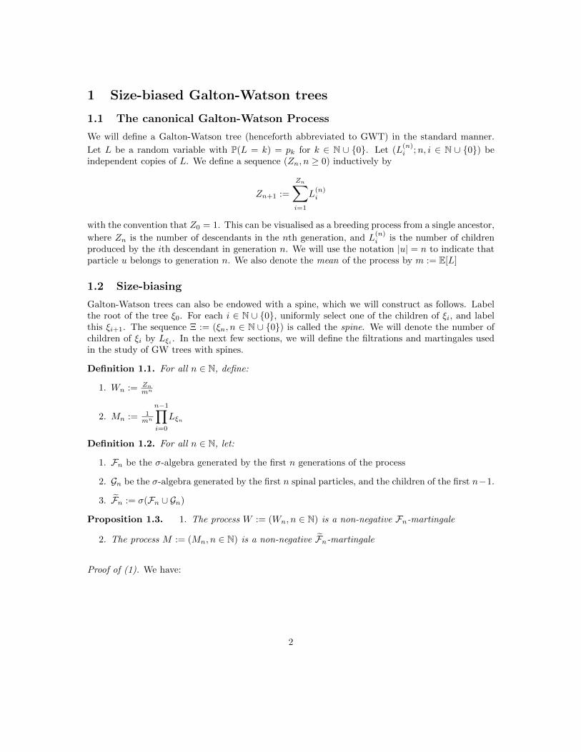
1 Size-biased Galton-Watson trees

1.1 The canonical Galton-Watson Process

We will define a Galton-Watson tree (henceforth abbreviated to GWT) in the standard manner.

Let L be a random variable with P(L = k) = pk for k ∈ N ∪ {0}. Let (L(n)i ;n, i ∈ N ∪ {0}) be

independent copies of L. We define a sequence (Zn, n ≥ 0) inductively by

Zn+1 :=

Zn∑i=1

L(n)i

with the convention that Z0 = 1. This can be visualised as a breeding process from a single ancestor,

where Zn is the number of descendants in the nth generation, and L(n)i is the number of children

produced by the ith descendant in generation n. We will use the notation |u| = n to indicate thatparticle u belongs to generation n. We also denote the mean of the process by m := E[L]

1.2 Size-biasing

Galton-Watson trees can also be endowed with a spine, which we will construct as follows. Labelthe root of the tree ξ0. For each i ∈ N ∪ {0}, uniformly select one of the children of ξi, and labelthis ξi+1. The sequence Ξ := (ξn, n ∈ N ∪ {0}) is called the spine. We will denote the number ofchildren of ξi by Lξi . In the next few sections, we will define the filtrations and martingales usedin the study of GW trees with spines.

Definition 1.1. For all n ∈ N, define:

1. Wn := Znmn

2. Mn := 1mn

n−1∏i=0

Lξn

Definition 1.2. For all n ∈ N, let:

1. Fn be the σ-algebra generated by the first n generations of the process

2. Gn be the σ-algebra generated by the first n spinal particles, and the children of the first n−1.

3. F̃n := σ(Fn ∪ Gn)

Proposition 1.3. 1. The process W := (Wn, n ∈ N) is a non-negative Fn-martingale

2. The process M := (Mn, n ∈ N) is a non-negative F̃n-martingale

Proof of (1). We have:

2

E[ Znmn

∣∣Fn−1

]= E

[1

mn

Zn−1∑i=1

L(n−1)i

∣∣∣∣Fn−1

]

=1

mn

Zn−1∑i=1

E[L

(n−1)i

∣∣Fn−1

]

=1

mn

Zn−1∑i=1

m =Zn−1

mn−1

Hence Wn is a martingale. Non-negativity is trivial.

Proof of (2) We have:

E[Mn|F̃n−1] =1

mnE[n−1∏i=0

Lξi

∣∣∣∣F̃n−1

]

=1

mn×n−2∏i=0

Lξi × E[Lξn−1 |F̃n−1]

=1

mn−1

n−2∏i=0

Lξi = Mn−1

Once again, non-negativity is trivial.

We will now use the martingale Mn to define a new probability measure, Q by setting:

dQdP

∣∣∣∣F̃n

= Mn

The following lemma and subsequent proposition will allow us to visualise how GW trees behaveunder this new measure.

Lemma 1.4. E[Mn|Fn] = Wn

Proof. From the definitions, we immediately have that E[Mn|Fn] = 1mnE[

∏n−1i=0 Lξn |Fn]. We now

sum over the indicator of j ∈ Ξ:

1

mnE[ Zn∑j=1

( n−1∏i=0

L(i)j

)1{j∈Ξ}

∣∣∣∣Fn]Now, both Zn and L

(i)j are Fn-measurable, and the indicator of j ∈ Ξ is independent of Fn. Hence

this reduces to

3

1

mn

Zn∑j=1

( n−1∏i=0

L(i)j

)P(j ∈ Ξ) =

The probability of any given j with |j| = n being a spinal particle is 1∏n−1i=0 Lξi

. The two products

now cancel out, leaving us with 1mn

∑Znj=1 1 = Zn

mn = Wn

Proposition 1.5. Let |u| = n. Then

Q(L(n)u = k) =

{kpkm u ∈ ξpk u 6∈ ξ

Proof. Consider u ∈ ξ. That is, u = ξn. Hence Q(L(n)u = k) = Q(Lξn = k) = E[Mn+11{Lξn+1

=k}].

The law of total expectation tells us that

E[Mn1{Lξn=k}] = E[Mn+1|Lξn = k]× P(Lξn = k)

= E[

k

mn+1

n−1∏i=0

Lξi

]× pk

=kpkmn+1

n−1∏i=0

E[Lξi ]

=kpkmn+1

×mn =kpkm

We now consider u 6∈ ξ. This gives us Q(L(n)u = k) = E[Mn+11{L(n)

u =k}]. Since u 6∈ ξ, we have

that Mn and the indicator function are independent. We can use this and reduce the expression to

E[Mn+1]P(L(n)u = k) = E[Mn+1]pk. We have as a corollary to Lemma 1.4 that E[Mn] = E[Wn] = 1,

completing the proof.

This proposition tells us that the offspring of particles in the spine follow a size-biased distribution,whereas the other particles behave in the usual manner. In particular, the probability of any spinalparticle having no children is 0. Since the root of the tree is in the spine, this tells us that under Q,the event of extinction almost surely does not occur. Lyons and Peres [2] call GWTs under the lawQ size-biased Galton-Watson trees. An example of a size-biased GWT is given in figure 1, whereeach non-spine particle forms the root of an independent GWT.

4

ξ0

ξ1

ξ2

ξ3

GW GW

GW

GW

Figure 1: An example tree after 4 generations

1.3 Spine Decomposition and the Kesten-Stigum theorem

We will now use the properties of sized-biased trees to prove Kesten and Stigum’s classic limittheorem, stated below.

Theorem 1.6. The Kesten-Stigum Theorem [1]Let L be the offspring random variable of a Galton-Watson process with mean m ∈ (1,∞) andmartingale limit W . Then the following are equivalent:

a. P[W = 0] = q

b. E[W ] = 1

c. E[L log+ L] <∞

Proposition 1.7. Spine DecompositionFor all n ≥ 1

EQ[Wn|G∞] =

n−1∑i=0

(Lξi − 1)m−(i+1) + 1

Proof. We will prove this result inductively. Since the root is also the first particle in the spine,we have that Z1 = Lξ0 . Therefore EQ[Wn|G∞] = 1

mLξ0 . This settles the base case. Now, we willconsider EQ[Wk+1|G∞] for some k > 1, which we will denote Ek+1. From the definitions of Wn andZn, we have that

Ek+1 =1

mk+1EQ

[ Zk∑i=0

L(k)i

∣∣∣∣G∞]

5

Now, under Q we know that there is exactly 1 spine particle in generation k, specifically ξk.Removing ξk’s children from the sum gives

1

mk+1EQ

[ Zk−1∑i=0

L(k)i + Lξk

∣∣∣∣G∞]We can now recall that Lξn is G∞-measurable, and use the iid nature of the L

(k)i s to rewrite this as

1

mk+1

((EQ[Zk|G∞]− 1)m+ Lξk

)=

1

mk+1

((mkEk − 1)m+ Lξk

).

The remaining steps are simply an exercise in algebraic manipulation. This proves the result.

Lemma 1.8. Let X1, X2, ... be a sequence of non-negative iid random variables. Then

lim supn→∞

1

nXn =

{0 if E[X] <∞∞ if E[X] =∞

almost surely.

Proof. We aim to use the Borel-Cantelli lemma to show that Xn/n is positive only finitely often. Todo this, we consider the event {Xnn ≥ ε} Since the Xn’s are iid, this event has the same probability

as {Xn ≥ ε}. We have:

∞∑k=1

P(X

k≥ ε)

=

∞∑k=1

P(X

ε≥ k

)=

∞∑k=1

E[1{X/ε≥k}] = E[ ∞∑k=1

1{X/ε≥k}

]= E

[bX/εc

].

Now by the Borel-Cantelli lemma, if E[X] < ∞ then the event {Xn/n ≥ ε} happens only finitelyoften for any ε > 0 (no matter how small), so Xn/n → 0. On the other hand, by the secondBorel-Cantelli lemma, if E[X] = ∞, then the event {Xn/n ≥ ε} happens infinitely often for anyε > 0 (no matter how large), so lim supn→∞Xn/n =∞.

Lemma 1.9. Let X1, X2, ... be a sequence of non-negative iid random variables. Then for anyc ∈ (0, 1),

∞∑k=1

eXkck

{<∞ if E[X] <∞=∞ if E[X] =∞

almost surely.

Proof. Suppose first that E[X] < ∞. By Lemma 1.8, we have that lim sup eXk/k = e0 = 1. Usingthe definition of limsup, we have that for all ε > 0, there exists an M such that eXk/k ≤ 1 + ε, foreach k ≥M . To prove our result, fix c ∈ (0, 1) and choose ε > 0 such that c(1 + ε) < 1. Then selectan M as above. Now:

∞∑k=M

eXkck ≤∞∑

k=M

(1 + ε)kck.

Since (1 + ε)c < 1, we have that the right hand side is finite. Finally, we write

∞∑k=1

eXkck =

M−1∑k=1

eXkck +

∞∑k=M

eXkck.

6

Since both of these sums are almost surely finite, we have proven the result in the case E[X] <∞.Now suppose E[X] =∞. By Lemma 1.8, lim supXn/n =∞, so for any K, we can find n1, n2, . . .→∞ such that Xni/ni ≥ K for all i. Fix c ∈ (0, 1), and choose ni as above with K = − log c. Then

∞∑n=1

eXncn ≥∞∑i=1

eXni cni ≥∞∑i=1

e−ni log ccni =

∞∑i=1

1 =∞

as required.

We will now use these two lemmas to prove that (c) implies (b) in the Kesten-Stigum theorem. Weneed one more tool, which is proved in [2].

Lemma 1.10. Suppose that µ and ν are probability measures and dµdν |Fn = Xn. Let X∞ =

lim supn→∞Xn. ThenX∞ <∞ ν-almost surely ⇔ Eµ[X∞] = 1

andX∞ =∞ ν-almost surely ⇔ Eµ[X∞] = 0.

We can now prove the Kesten-Stigum thoerem.

Proposition 1.11. Let W and L be as in Theorem 1.6. Then:

E[L log+ L] <∞⇔ E[W ] = 1

Proof. We first show that 1/Wn is a supermartingale under Q. Recall from the definition thatEQ[1/Wn|Fn−1] is the (almost surely unique) Fn−1-measurable random variable Y such that EQ[1/Wn1A] =EQ[Y 1A] for all A ∈ Fn−1. Now,

EQ[1

Wn1A] = EP[1A1{Wn>0}] = EP[1A1{Wn−1>0}P(Wn > 0|Fn−1)] = EQ[

1

Wn−11AP(Wn > 0|Fn−1)].

Therefore

EQ[1

Wn|Fn−1] =

1

Wn−1P(Wn > 0|Fn−1) ≤ 1

Wn−1.

So 1/Wn is a non-negative supermartingale under Q, so it converges almost surely to a limit 1/W∞(which may be 0). In particular, lim supn→∞Wn = lim infn→∞Wn, Q-almost surely.Now we demonstrate that lim supn→∞ EQ[Wn|G∞] is almost surely finite if E[L log+ L] <∞. FromLemma 1.7, we have that

EQ[Wn|G∞] = 1 +

n−1∑i=0

(Lξi − 1)m−(i+1)

≤ 1 +

n∑i=1

elog+(Lξi−1−1)m−i

Clearly, by Lemma 1.9 this converges when EQ[log+(Lξi − 1)] < EQ[log+(Lξi)] <∞. Now,

7

EQ[log+(Lξi)] =

∞∑k=0

Q(Lξi = k) log+ k

=

∞∑k=0

kpkm

log+ k

=1

mE[L log+ L]

Hence, E[L log+ L] < ∞ =⇒ lim supEQ[Wn|G∞] < ∞ almost surely. Now Fatou’s lemma,combined with the fact (proven above) that lim supn→∞Wn = lim infn→∞Wn, Q-almost surely,gives

EQ[lim supWn|G∞] = EQ[lim inf Wn|G∞] ≤ lim inf EQ[lim inf Wn|G∞] ≤ lim supEQ[lim inf Wn|G∞] <∞.

Therefore lim supWn <∞ Q-almost surely, so by Lemma 1.10 we have EP[W ] = 1.

2 A discrete-time branching process on the unit square

2.1 Preliminaries and heuristics

Our process begins with the unit square. It splits into two rectangles of area U and 1− U respec-tively, where U is a random variable uniform on [0, 1]. In each subsequent generation, each of therectangles splits in a manner similar to the original square. The orientation of these splits is notrelevant to the following results, so we assume that each split occurs either vertically or horizontallywith probability 1

2 . Figure 2 shows a simulated outcome of this process after ten generations.

A natural question to ask is: what size would we expect the smallest and largest rectangles to beafter n generations? There are many ways one could interpret the notion of size in this context;for our purposes, we will be considering the area of each rectangle to be its size. After n ≥ 1generations, the area of any given rectangle in the nth generation, here denoted An, can be written:

An =

n∏k=1

Uk

where (Uk : k ∈ N) is a sequence of iid unif(0, 1) random variables. We will denote the set ofrectangles in generation n by Nn.

We will now use our simulation to plot the areas of the rectangles in each generation, and hopefullyprovide some heuristic justification for the main result of this paper.

8

Figure 2: The process after 10 generations

9

Here we see what our intuition tells us: the area of the rectangles decreases exponentially quickly.This plot however is not particularly useful due to the nature of exponential growth. To rectifythis, we will plot the logarithm of the area of each rectangle.

Clearly, the growth of the log-area in this plot is linear, somewhat confirming our suspicion thatthe growth is exponential. It also appears that there are upper and lower boundary lines betweenwhich all of the rectangles fall. It is the upper boundary line which, over the course of this sec-tion, we shall not only demonstrate the existence of, but also give an explicit expression for its slope.

Before we do this, we shall construct a spine for this process in a manner very similar to that inSection 1.3. We will henceforth refer to the rectangles as particles. As before, we shall define thespine recursively. Define ξ0 as the root particle. For each ξk, uniformly select one of its children,and set that particle to be ξk+1. Finally, define Ξ = {ξk|k ∈ N0}. This forms our spine.

2.2 Change of measure and Spine Decomposition

Definition 2.1. Important filtrations

1. Fn is the filtration defined by the first n generations of the process

2. Gn is the filtration defined by the first n generations of the spine

3. F̃n = σ(Fn ∪Gn)

10

Proposition 2.2. Let α > −1. Then:

1. The process W (α) = (W(α)n )n∈N defined by W

(α)n = (α+1

2 )n∑u∈Nn A

αu is a Fn-martingale

2. The process M = (Mn)n∈N defined by Mn = Aαξn(α+ 1)n is a F̃n-martingale

We now define a new measure Q by setting dQdP∣∣F̃n

= Mn. In the following propositions, we willshow that the spine decomposition converges Q almost-surely to a finite limit. First, we need toconsider how our process changes under this new measure.

Lemma 2.3. Let u ∈ Nn. Then for all k ∈ [0, 1] and β ∈ N:

(i) Q(Uu ≤ x) =

{xα+1 u ∈ Ξ

x u 6∈ Ξ

(ii) EQ[Uβu ] =

{α+1

α+β+1 u ∈ Ξ1

β+1 u 6∈ Ξ

(iii) EQ[logUξn ] = − 1α+1

Proof. Consider the case that u ∈ Ξ. Then u = ξn, and:

Q(Uξn ≤ x) = E[Mn|Uξn ≤ x]× P(Uξn ≤ x)

= x(α+ 1)n × E[Aαξn−1Uαξn |Uξn ≤ x]

= x(α+ 1)n × E[Aαξn−1]× E[Uαξn |Uξn ≤ x]

= x(α+ 1)n × 1

(a+ 1)n−1×∫ x

0

1

xxα dx

= x(α+ 1)× 1

x× xα+1

α+ 1

= xα+1

Define gu(x) to be the pdf of Uu under Q. Let u = ξn. We now know that

gξn(x) :=dQ(Uξn ≤ x)

dx= (α+ 1)xα

Hence,

EQ[Uβu ] = (α+ 1)

∫ 1

0

xα+βdx

=α+ 1

α+ β + 1

As required. The results for u 6∈ Ξ are trivial. Finally, we have:

EQ[logUξn ] = (α+ 1)

∫ 1

0

log(x)xαdx

= − α+ 1

(α+ 1)2= − 1

α+ 1

11

Proposition 2.4. The Spine DecompositionLet α ∈ [0, 1]. Then:

EQ

[W (α)n

∣∣∣G∞] = Aαξn

(α+ 1

2

)n+

(α+ 1

2

) n−1∑k=0

(α+ 1

2

)k (Aξk −Aξk+1

)αProof. Let us consider what particles exist at time n. A trivial examination of this tree structurereveals that for any k < n, there will be 2n−k−1 particles alive at time n whose last spinal ancestorwas ξk. We will denote the set of non-spine descendants of ξk alive at time n by Cn(ξk). Each

u ∈ Cn(ξk) has size distribution Aξk×∏n−k

Ui, where the Ui’s are uniform (0, 1) random variables.Now, we can once again use the binary structure of the process to remove a degree of randomnessfrom this expression. ξk has two children. One of these children is in the spine, and hence contributesno descendants to Cn(ξk). However, the other child has size distribution Aξk+1

− Aξk , and itsdescendants at time n form precisely the set Cn(ξk). As such, each u ∈ Cn(ξk) has distribution

(Aξk+1− Aξk)×

∏n−k−1Ui. The keen observer will notice however that |

⋃k Cn(ξk)| = 2n − 1; we

are missing ξn, which trivially has size distribution Aξn . This completes our characterisation of theparticles in Nn. Hence:

EQ

[W (α)n |G∞

]=

(α+ 1

2

)n×

(EQ[Aαξn |G∞

]+

n−1∑k=0

2n−k−1EQ

[((Aξk+1

−Aξk)×n−k−1∏i=1

Ui

)α ∣∣∣∣G∞])

Now, the Aξk ’s are G∞-measurable, so we can take them out of the expectations. The Ui’s are alsoindependent of G∞, so we simply take their Q-expectations. By Proposition 2.3.(ii), we have thatEQ [Uαi ] = 1

α+1 . Hence our full expression for the spine decomposition is

EQ

[W (α)n |G∞

]=

(α+ 1

2

)n×

(Aαξn +

n−1∑k=0

(2

α+ 1

)n−k−1 (Aξk+1

−Aξk)α)

some simple algebraic manipulation gives the required result.

Proposition 2.5. Set α such that e−αα+1 < (α+1

2 ). Then:

lim supEQ[W (α)n |G∞] <∞

almost surely.

Proof. First we will consider the convergence of∑∞k=0

(α+1

2

)k (Aξk −Aξk+1

)α. We will first rewrite

this as∑∞k=0

[(α+1

2

)eαk log(Aξk−Aξk+1)

]k. We have that:

1

klog(Aξk −Aξk+1

)=

1

klog

((1− Uξk+1

) k∏i=0

Uξi

)

=log(1− Uξk+1

)

k+

1

k

k∑i=1

log(Uξi)

12

We now have two summands to consider. By the SLLN, 1k

∑ki=1 logUξi → EQ[logUξi ] Q-almost

surely. By Lemma 2.3 we know that this is − 1α+1 . We will now consider the convergence of

1k log(1 − Uξk+1

). By Lemmas 1.8 and 2.3, we have that − 1k log(1 − Uξk+1

) converges to 0. Hencewe also have 1

k log(1− Uξk+1)→ 0, Q-almost-surely. This gives us a precise limit:

limk→∞

1

klog(Aξk −Aξk+1

)= − 1

α+ 1

Hence, we have that

limk→∞

(α+ 1

2

)exp

(αk

log(Aξk −Aξk+1

))=

(α+ 1

2

)e−

αα+1

We have now that the sum∑∞k=0

(α+1

2

)k (Aξk −Aξk+1

)αconverges Q-almost surely if (α+1

2 )e−αα+1 <

1. It remains now to find which values of α ensure the convergence of Aαξn(α+1

2

)n. Now:

limn→∞

1

nlog(Aξn) = lim

n→∞

1

nlog

(n∏i=1

Uξi

)

= limn→∞

1

n

n∑i=1

log(Uξn)

= EQ[logUξn ] = − 1

α+ 1

Hence, similar to before,

lim supn→∞

(α+ 1

2

)nAαξn = lim sup

n→∞

[(α+ 1

2

)eαn log(Aξn )

]n= lim sup

n→∞

[(α+ 1

2

)e−

αα+1

]nWhich is finite iff (α+1

2 )e−αα+1 < 1. This fact, combined with the convergence of the aforementioned

sum on the same interval gives us our required condition for convergence.

2.3 Asymptotic growth of the maximal particle

The following three lemmas are essential in proving our main result.

Lemma 2.6. Set α such that e−αα+1 < (α+1

2 ). Then:

E[

limn→∞

W (α)n

]= 1

Q(α)-almost surely.

Proof. We first use the proof of Proposition 1.11 to deduce that lim supn→∞W(α)n = lim infn→∞W

(α)n .

We now have

EQ[lim supW (α)n |G∞] = EQ[lim inf W (α)

n |G∞] ≤ lim inf EQ[W (α)n |G∞] ≤ lim supEQ[W (α)

n |G∞] <∞

From a combination of Fatou’s Lemma and Proposition 2.5. Therefore, limW(α)n < ∞ Q-almost

surely, and by Lemma 1.10 we have that E[limn→∞W

(α)n

]= 1 as required.

13

Lemma 2.7. Let A ∈ Fn. Then:

Q(α)(A) = EP

[W (α)∞ 1E

]+ P(A ∩ {W (α)

∞ =∞})

Proof is a standard result of measure theory

Lemma 2.8. Let Eδ be the event {supu∈Nn1n logAu > δ i.o.}. Then P(Eδ) is either 0 or 1.

Proof. We shall consider the probability of the complement of Eδ given the filtration Fk.We have that:

P(Ecδ |Fk) = P(∀v ∈ Nk, sup

u∈Nn, v≤u

logAun

≤ δ e.v.

∣∣∣∣Fk)= P

( ⋂v∈Nk

{sup

u∈Nn, v≤u

logAun

≤ δ e.v.

} ∣∣∣∣Fk)

=∏v∈Nk

P(

supu∈Nn, v≤u

logAun

≤ δ e.v.

∣∣∣∣Fk)

=∏v∈Nk

P

(sup

u∈Nn−k

logAun

≤ δ e.v.

)

=∏v∈Nk

P(

supu∈Nn

logAun

· n+ k

n≤ δ e.v.

)≤∏v∈Nk

P(

supu∈Nn

logAun

≤ δ + ε e.v.

)= P

(Ecδ+ε

)|Nk|To summarise, we now have that P(Ecδ |Fk) ≤ P(Ecδ+ε)

|Nk|. We can now take the limit as ε→ 0 and

take the expectation of both sides to obtain P(Ecδ) ≤ P(Ecδ)2k . This proves the result.

The following definition and lemma are purely technical, serving only to simplify the statement ofthe main theorem.

Definition 2.9. The Lambert W FunctionLet z be any complex number. Then W is the unique function satisfying the equation

z = W (z)eW (z)

Lemma 2.10.

minx>0

(1

xlog

2

x+ 1

)= W

(− 1

2e

)Proof. Let f(x) = 1

x log 2x+1 . Simple calculus shows that

f ′(x) = − 1

x2log

2

x+ 1− 1

x(x+ 1)

14

setting f ′(x) = 0, we obtain1

xlog

2

x+ 1= − 1

x+ 1(1)

Let x∗ denote the solution to this equation, and let f∗ denote the minimum of f . Then clearly f∗

is given by

f∗ = f(x∗) = − 1

x∗ + 1

Rearranging (1), we can obtain

− 1

2e= − 1

x+ 1e−

1x+1

Hence the f∗ is the solution to the equation

− 1

2e= f∗ef

∗

The definition of the Lambert W Function says that for any real number z, we have

z = W (z)eW (z)

Therefore, f∗ = W (− 12e )

Theorem 2.11. Let both Au and Nn be defined as in Section 2.1. Then,

lim supn→∞

(maxu∈Nn

logAun

)= W

(− 1

2e

)Almost surely.

Proof. This proof is split into two parts, in which we will derive both upper and lower bounds forthe limit. We will begin with the former. Fix some γ ∈ R, and suppose that there exists someparticle u ∈ Nn such that logAu

n > γ. Then,

W (α)n =

(α+ 1

2

)n ∑v∈Nn

Aαu ≥(α+ 1

2

)nAαu >

(α+ 1

2

)neαγn

Now, since W(α)n is a non-negative martingale, it converges almost surely to a finite limit. Hence

to ensure convergence, we must have that(α+1

2

)eαγ > 1 only finitely often. Rewriting this, we

see that this implies maxu∈NnlogAun > γ > 1

α log 2α+1 happens only finitely often for all α > 0.

This inequality relies on varying α, so we will optimise over α via Lemma 2.10, giving us thatminα>0

1α log 2

α+1 = W (− 12e ) Therefore, we have

lim supn→∞

(maxu∈Nn

logAun

)≤W

(− 1

2e

)almost surely.

Now, we will use our spine decomposition to provide the lower bound. Let W(α)∞ := lim supW

(α)n .

By Lemma 2.6 we have that E[W(α)∞ ] = 1. Hence P(W

(α)∞ = ∞) = 0. Now, combining this with

Lemma 2.7, we have

15

Q(α)(A) = EP

[W (α)∞ 1A

]Let E be the event {supu∈Nn

1n logAu ≥ − 1

α+1 i.o.}. In Proposition 2.5, we showed that limn→∞1n logAξn =

− 1α+1 , i.e. Q(α){ 1

n logAξn = − 1α+1 i.o.} = 1. The following sequence of set inclusions will make it

obvious that Q(α)(E) = 1:

{1

nlogAξn = − 1

α+ 1i.o.

}⊆{

1

nlogAξn ≥ −

1

α+ 1i.o.

}⊆{

supu∈Nn

1

nlogAu ≥ −

1

α+ 1i.o.

}= E

We also have that

Q(α)(E) = EP

[W (α)∞ 1E

]Hence P(E) > 0. Finally, by Lemma 2.8 we have that P(E) = 0 or 1. We have just shown thatP(E) > 0, therefore we necessarily have that P(E) = 0, i.e.

lim supn→∞

(supu∈Nn

logAun

)≥ − 1

α+ 1= W

(− 1

2e

)Proving our result.

References

[1] H. Kesten and B. P. Stigum. A limit theorem for multidimensional galton-watson processes.Ann. Math. Statist., 37(5):1211–1223, 10 1966.

[2] R. Lyons and Y. Peres. Probability on Trees and Networks. Cambridge University Press, 2016.

16