Basics of Multivariate Modelling and Data Analysis · 2.2.1.1 Principal component analysis (PCA)...

KEH Basics of Multivariate Modelling and Data Analysis 1

Basics of Multivariate Modelling and Data Analysis Kurt-Erik Häggblom

2. Overview of multivariate techniques 2.1 Different approaches to multivariate data analysis 2.2 Classification of multivariate techniques


2. Overview of multivariate techniques

2.1 Different approaches to multivariate data analysis Two main approaches Essentially, there are two different approaches: Model-driven approach, where data is seen as realizations of random

variables of an underlying statistical model. This interpretation is usually favoured by statisticians.

Data-driven approach, where the statistical tools are basically seen as algorithms to obtain results. This view is typical of chemometricians and data miners.

However, these are not two different ways for solving the same problem. Traditional statistical (model-driven) methods do not work well when the statistical properties are unknown (i.e. assumptions are not fulfilled) the number of variables is “large” compared to the number of objects

(samples, observations, measurements), sometimes larger than the variables are strongly correlated

Data-driven methods are developed to handle this kind of data.


2. Overview of multivariate techniques 2.1 Different approaches…

Chemometrics Chemometrics is the science of extracting information from chemical systems (chemistry,

biochemistry, chemical engineering, etc.) by data-driven means a highly cross-disciplinary activity using methods from applied

mathematics, statistics, informatics and computer science applied to datasets which are often very large and highly complex,

involving hundreds to tens of thousands of variables, and hundreds to millions of cases or observations

applied to solve both descriptive and predictive problems – descriptive application: modelling with the intent of learning the underlying

relationships and structure of the system (i.e. model identification) – predictive application: modelling with the intent of predicting new

properties or behaviour of interest

We will mainly deal with applications of chemometrics in this course.


2. Overview of multivariate techniques 2.1 Different approaches…

Data mining Data mining is the science of extracting information from large data sets and databases an integration of techniques from statistics, mathematics, machine

learning, database technology, data visualization, pattern recognition, signal processing, information retrieval, high-performance computing,…

often applied to huge data sets involving gigabytes (230~109 bytes; the Human Genome Project), terabytes (240~1012 bytes; space and earth sciences), soon even petabytes (250~1015 bytes)

applied to solve both descriptive and predictive problems – descriptive data mining (or unsupervised learning): search massive data sets

and discover the locations of unexpected structures or relationships, patterns, trends, clusters and outliers

– predictive data mining (or supervised learning): build models and procedures for regression, classification, pattern recognition and machine learning tasks; assess the predictive accuracy of those methods when applied to new data

Obviously, data mining methods are also used in chemometrics.


2. Overview of multivariate techniques

2.2 Classification of multivariate techniques

1x 2x px

11x21x

1nx

12x22x

1px2 px

2nx npx

X =

1y 2y qy

11y21y

1ny

12y22y

1qy2qy

2ny nqy

Y =

Data matrices Data is assumed to be available in a data matrix 𝑋, where each column 𝒙𝑗 , 𝑗 = 1, … ,𝑝 , contains 𝑛 observations (measurements). Each column in 𝑋 represents a variable and each row contains measure-ments of all variables in a sample (or time instant). These variables are termed independent variables (although they may be highly correlated).

In addition there may be data of a number of depen-dent variables in a matrix 𝑌 , where each column 𝒚𝑘 , 𝑘 = 1, … , 𝑞 , contains 𝑛 observations. Each column in 𝑌 represents a variable and each row contains measurements of all dependent variables in a sample (or time instant).


2. Overview of multivariate techniques 2.2 Classification…

Main classification criterion Our main classification criterion is the number of dependent variables. The classes are no dependent variable, 𝑞 = 0 one dependent variable, 𝑞 = 1 many dependent variables, 𝑞 > 1

Note that this classification is determined by how we choose to treat the data, not by the “true” (unknown) dependencies in the data set.

Modelling (like regression) is termed simple, if there is only one independent variable (e.g. simple regression) multiple, if there is one dependent variable but many independent ones multivariate, if there is many dependent and many independent variables

The case with one independent variable is handled by classical univariate statistics, and will not be treated here.

In addition, variables may be classified according to the type of measurement: metric (quantitative, ~ continuous) nonmetric (qualitative, categorical, discrete, often binary)



2.2.1 No dependent variable In these methods, only the data matrix 𝑋 is considered. The data may be metric or nonmetric.

2.2.1.1 Principal component analysis (PCA)

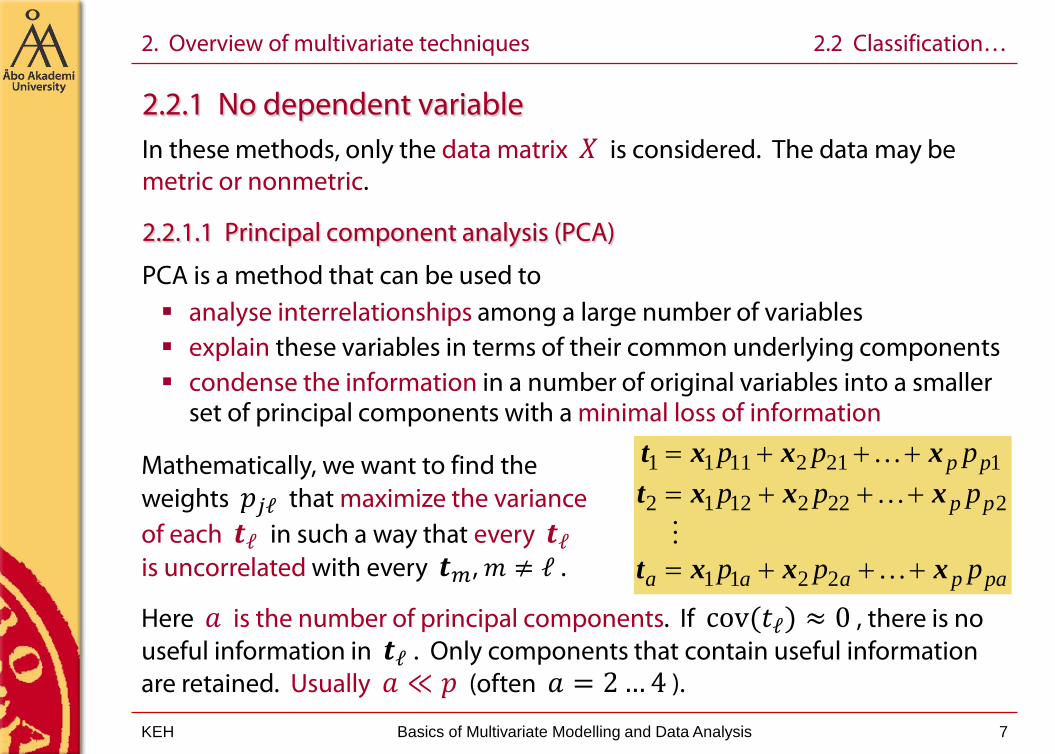
PCA is a method that can be used to analyse interrelationships among a large number of variables explain these variables in terms of their common underlying components condense the information in a number of original variables into a smaller

set of principal components with a minimal loss of information

1 1 11 2 21 1

2 1 12 2 22 2

1 1 2 2

p p

p p

a a a p pa

p p pp p p

p p p

= + + += + + +

= + + +

t x x xt x x x

t x x x

Mathematically, we want to find the weights 𝑝𝑗ℓ that maximize the variance of each 𝒕ℓ in such a way that every 𝒕ℓ is uncorrelated with every 𝒕𝑚, 𝑚 ≠ ℓ .

Here 𝑎 is the number of principal components. If cov(𝑡ℓ) ≈ 0 , there is no useful information in 𝒕ℓ . Only components that contain useful information are retained. Usually 𝑎 ≪ 𝑝 (often 𝑎 = 2 … 4 ).


2.2 Classification of multivariate techniques 2.2.1 No dependent variable

2.2.1.2 Factor analysis (FA)

Factor analysis is similar to PCA and can be used for the same purpose. However, unlike PCA, FA is based on a statistical model with certain assumptions.

FA FA FA FA FA FA

FA FA FA FA FA FA

FA FA FA FA FA FA

1 11 1 12 2 1 1

2 21 1 22 2 2 2

1 1 2 2

a a

a a

p p p pa a p

p p p

p p p

p p p

= + + + +

= + + + +

= + + + +

x t t t e

x t t t e

x t t t e

Mathematically, we want to find the weights 𝑝𝑗ℓFA and the factors 𝒕ℓFA so that the error variance behaves in a certain way.

Example. Consumer rating. Assume customers in a fast-food restaurant are asked to rate the restaurant on the following six variables: food taste, food temperature, food freshness, waiting time, cleanliness, friendliness of employees. Analysis of the customer responses by factor analysis may show that the variables food taste, temperature and freshness combine together to form a single factor “food quality”, whereas waiting time, cleanliness and friendliness form a factor “service quality”.


2.2 Classification of multivariate techniques 2.2.1 No dependent variable

2.2.1.3 Cluster analysis (FA)

Cluster analysis is an analytical technique for developing meaningful subgroups of individuals or objects. The subgroups are not predefined; they are identified by the analysis.



2.2.2 One dependent variable

In these methods, a vector of dependent variables, 𝑌 = 𝒚 , is considered in addition to the data matrix 𝑋 . The data my be metric or nonmetric.

2.2.2.1 Multiple regression analysis (MRA)

MRA may be used to relate a single metric dependent variable to a number of independent

variables. predict changes in the dependent variable in response to changes in the

independent variables.

Mathematically, we want to find the parameters 𝑏𝑗 , 𝑗 = 0, … , 𝑝 , that maximize the correlation between 𝒚 and the prediction 𝒚� .

0 1 1 2 2

0 1 1 2 2ˆ

p p

p p

b b b b

b b b b

= + + + + +

= + + + +

y x x x e

y x x x

This is equivalent to minimizing the variance of the error 𝒆 or the sum of the squared residuals.

Note: This method does not work well if the independent variables are (strongly) correlated.


2.2 Classification of multivariate techniques 2.2.2 One dependent variable

2.2.2.2 Multiple discriminant analysis (MDA)

MDA is the appropriate multivariable technique if the single dependent variable 𝒚 is nonmetric, either dichotomous (e.g., male–female), or multichotomous (e.g. , high–medium–low).

The independent variables 𝒙𝑗 are assumed to be metric.

Thus, discriminant analysis is applicable when the total sample can be divided into groups based on a nonmetric dependent variable characterizing several known classes. The primary objectives of MDA are to understand groups differences predict the likelihood that an entity (individual or object) will belong to a

particular class or group based on several metric independent variables


2.2 Classification of multivariate techniques 2.2.2 One dependent variable

2.2.2.3 Logistic regression

Logistic regression models, often referred to as logit analysis, are a combination of multiple regression analysis (MRA) — many independent variables multiple discriminant analysis (MDA) — nonmetric dependent variable

The difference with these methods is that the independent variables may be may be metric or nonmetric do not require the assumption of multivariate normality

In many cases, particularly with more than two levels of the dependent variable, MDA is the more appropriate technique.



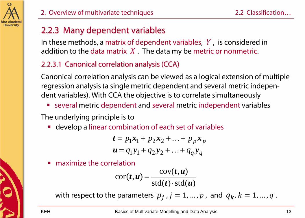
2.2.3 Many dependent variables In these methods, a matrix of dependent variables, 𝑌 , is considered in addition to the data matrix 𝑋 . The data my be metric or nonmetric.

2.2.3.1 Canonical correlation analysis (CCA)

Canonical correlation analysis can be viewed as a logical extension of multiple regression analysis (a single metric dependent and several metric indepen-dent variables). With CCA the objective is to correlate simultaneously several metric dependent and several metric independent variables

The underlying principle is to develop a linear combination of each set of variables

maximize the correlation

with respect to the parameters 𝑝𝑗 , 𝑗 = 1, … , 𝑝 , and 𝑞𝑘 , 𝑘 = 1, … , 𝑞 .

1 1 2 2

1 1 2 2

p p

q q

p p pq q q

= + + += + + +

t x x xu y y y

cov( , )cor( , )std( ) std( )

=⋅t ut u

t u


2.2 Classification of multivariate techniques 2.2.3 Many dependent variables

2.2.3.2 Partial least squares (PLS) PLS stands for Partial Least Squares, or Projection to Latent Structures

It is a method to relate a matrix 𝑋 to a vector 𝒚 or a matrix 𝑌. Similarly to CCA, linear combinations of the 𝑋 and 𝑌 data are formed: In PLS, 𝑝𝑗ℓ , 𝑗 = 1, … , 𝑝, and 𝑞𝑘𝑚 , 𝑘 = 1, … , 𝑞, are (usually) determined so that the covariances between 𝒕ℓ and 𝒖𝑚, ∀ℓ,𝑚 , are maximized. This combines high variance of 𝒕ℓ and 𝒖𝑚 (i.e., high information content) high correlation between 𝒕ℓ and 𝒖𝑚 (good for predictive modelling)

In addition, linear relationships between 𝒕ℓ and 𝒖𝑚 are determined by ordinary least squares (OLS).

There is a similar method, principal component regression (PCR), where 𝑝𝑗ℓ , 𝑗 = 1, … ,𝑝, are determined by principal component analysis (PCA) of 𝑋.

1 1 2 2

1 1 2 2

, 1, ,, 1, ,

p p

m m m q qm

p p p aq q q m b

= + + + == + + + =

t x x xu y y y


2.2 Classification of multivariate techniques 2.2.3 Many dependent variables

2.2.3.3 Independent component analysis (ICA) In general, ICA tries to reveal the independent factors (variables/signals) from a set of mixed random variables or measurement signals. ICA is typically restricted to linear mixtures, and the underlying sources are assumed to be mutually independent. This is a stronger assumption than no correlation (which only concerns the first two moments of probability distributions)!

It is assumed that the observed random variables 𝒙1, … ,𝒙𝑝, denoted by the observation matrix 𝑋, are the result of a linear combination of 𝑚 underlying sources 𝒔1, … , 𝒔𝑚 , denoted by the source matrix 𝑆. The following model, called a noise-free ICA model, can then be assumed:

𝑋 = 𝐴𝑆T Here 𝐴 is a full rank 𝑛 × 𝑚 matrix, where 𝑛 is the number of observations.

Both 𝐴 and 𝑆 are unknown, but if the sources are statistically independent , it is possible to find 𝐴. The sources are then found according to

𝑆T = 𝐴−1𝑋

Basics of Multivariate Modelling and Data Analysis · 2.2.1.1 Principal component analysis (PCA)...

Documents

Transcript of Basics of Multivariate Modelling and Data Analysis · 2.2.1.1 Principal component analysis (PCA)...