Basic Principles of Statistical Inference · Probability theory used to model stochastic events...

Basic Principles of Statistical Inference

Kosuke Imai

Department of PoliticsPrinceton University

POL572 Quantitative Analysis IISpring 2016

Kosuke Imai (Princeton) Basic Principles POL572 Spring 2016 1 / 66

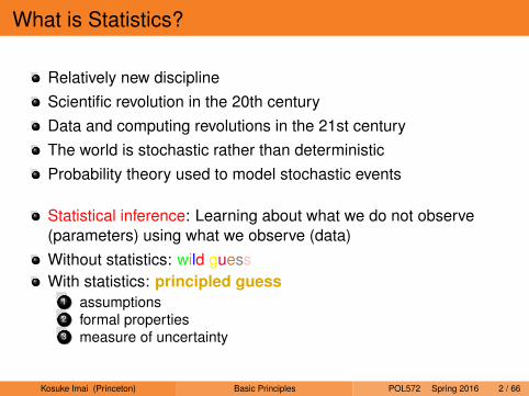
What is Statistics?

Relatively new disciplineScientific revolution in the 20th centuryData and computing revolutions in the 21st centuryThe world is stochastic rather than deterministicProbability theory used to model stochastic events

Statistical inference: Learning about what we do not observe(parameters) using what we observe (data)Without statistics: wild guessWith statistics: principled guess

1 assumptions2 formal properties3 measure of uncertainty


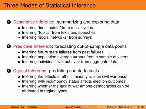
Three Modes of Statistical Inference

1 Descriptive Inference: summarizing and exploring dataInferring “ideal points” from rollcall votesInferring “topics” from texts and speechesInferring “social networks” from surveys

2 Predictive Inference: forecasting out-of-sample data pointsInferring future state failures from past failuresInferring population average turnout from a sample of votersInferring individual level behavior from aggregate data

3 Causal Inference: predicting counterfactualsInferring the effects of ethnic minority rule on civil war onsetInferring why incumbency status affects election outcomesInferring whether the lack of war among democracies can beattributed to regime types


Statistics for Social Scientists

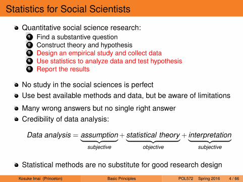
Quantitative social science research:1 Find a substantive question2 Construct theory and hypothesis3 Design an empirical study and collect data4 Use statistics to analyze data and test hypothesis5 Report the results

No study in the social sciences is perfectUse best available methods and data, but be aware of limitations

Many wrong answers but no single right answerCredibility of data analysis:

Data analysis = assumption︸︷︷︸subjective

+ statistical theory︸︷︷︸objective

+ interpretation︸︷︷︸subjective

Statistical methods are no substitute for good research design


Sample Surveys


Sample Surveys

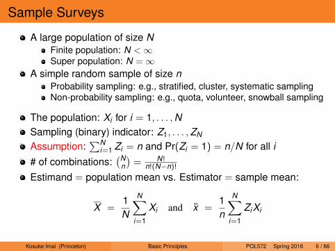
A large population of size NFinite population: N <∞Super population: N =∞

A simple random sample of size nProbability sampling: e.g., stratified, cluster, systematic samplingNon-probability sampling: e.g., quota, volunteer, snowball sampling

The population: Xi for i = 1, . . . ,NSampling (binary) indicator: Z1, . . . ,ZN

Assumption:∑N

i=1 Zi = n and Pr(Zi = 1) = n/N for all i# of combinations:

(Nn

)= N!

n!(N−n)!

Estimand = population mean vs. Estimator = sample mean:

X =1N

N∑i=1

Xi and x̄ =1n

N∑i=1

ZiXi


Estimation of Population Mean

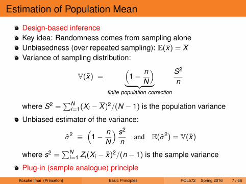
Design-based inferenceKey idea: Randomness comes from sampling aloneUnbiasedness (over repeated sampling): E(x̄) = XVariance of sampling distribution:

V(x̄) =(

1− nN

)︸︷︷︸

finite population correction

S2

n

where S2 =∑N

i=1(Xi − X )2/(N − 1) is the population variance

Unbiased estimator of the variance:

σ̂2 ≡(

1− nN

) s2

nand E(σ̂2) = V(x̄)

where s2 =∑N

i=1 Zi(Xi − x̄)2/(n − 1) is the sample variance

Plug-in (sample analogue) principle


Some VERY Important Identities in Statistics

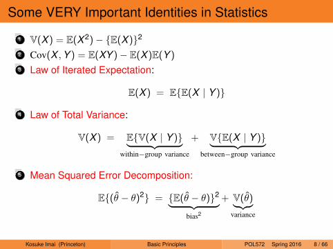
1 V(X ) = E(X 2)− {E(X )}22 Cov(X ,Y ) = E(XY )− E(X )E(Y )

3 Law of Iterated Expectation:

E(X ) = E{E(X | Y )}

4 Law of Total Variance:

V(X ) = E{V(X | Y )}︸︷︷︸within−group variance

+ V{E(X | Y )}︸︷︷︸between−group variance

5 Mean Squared Error Decomposition:

E{(θ̂ − θ)2} = {E(θ̂ − θ)}2︸︷︷︸bias2

+ V(θ̂)︸︷︷︸variance


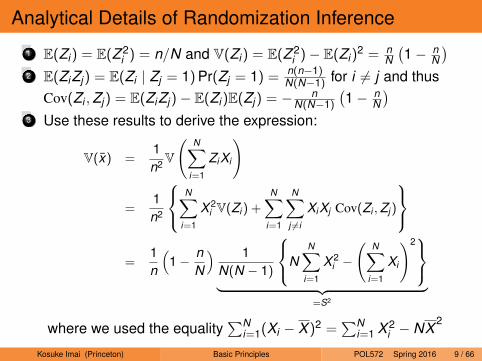
Analytical Details of Randomization Inference

1 E(Zi) = E(Z 2i ) = n/N and V(Zi) = E(Z 2

i )− E(Zi)2 = n

N

(1− n

N

)2 E(ZiZj) = E(Zi | Zj = 1) Pr(Zj = 1) = n(n−1)

N(N−1) for i 6= j and thusCov(Zi ,Zj) = E(ZiZj)− E(Zi)E(Zj) = − n

N(N−1)

(1− n

N

)3 Use these results to derive the expression:

V(x̄) =1n2V

(N∑

i=1

ZiXi

)

=1n2

N∑

i=1

X 2i V(Zi ) +

N∑i=1

N∑j 6=i

XiXj Cov(Zi ,Zj )

=

1n

(1− n

N

) 1N(N − 1)

NN∑

i=1

X 2i −

(N∑

i=1

Xi

)2︸︷︷︸

=S2

where we used the equality∑N

i=1(Xi − X )2 =∑N

i=1 X 2i − NX

2


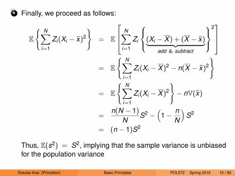
4 Finally, we proceed as follows:

E

{N∑

i=1

Zi(Xi − x̄)2

}= E

N∑i=1

Zi

(Xi − X ) + (X − x̄)︸︷︷︸add & subtract

2

= E

{N∑

i=1

Zi(Xi − X )2 − n(X − x̄)2

}

= E

{N∑

i=1

Zi(Xi − X )2

}− nV(x̄)

=n(N − 1)

NS2 −

(1− n

N

)S2

= (n − 1)S2

Thus, E(s2) = S2, implying that the sample variance is unbiasedfor the population variance


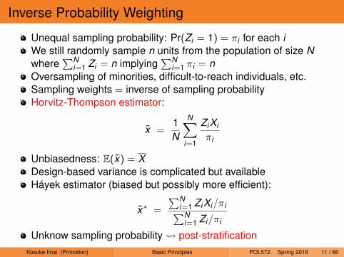
Inverse Probability Weighting

Unequal sampling probability: Pr(Zi = 1) = πi for each iWe still randomly sample n units from the population of size Nwhere

∑Ni=1 Zi = n implying

∑Ni=1 πi = n

Oversampling of minorities, difficult-to-reach individuals, etc.Sampling weights = inverse of sampling probabilityHorvitz-Thompson estimator:

x̃ =1N

N∑i=1

ZiXi

πi

Unbiasedness: E(x̃) = XDesign-based variance is complicated but availableHáyek estimator (biased but possibly more efficient):

x̃∗ =

∑Ni=1 ZiXi/πi∑N

i=1 Zi/πi

Unknow sampling probability post-stratificationKosuke Imai (Princeton) Basic Principles POL572 Spring 2016 11 / 66

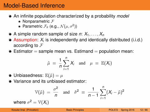
Model-Based Inference

An infinite population characterized by a probability modelNonparametric FParametric Fθ (e.g., N (µ, σ2))

A simple random sample of size n: X1, . . . ,Xn

Assumption: Xi is independently and identically distributed (i.i.d.)according to FEstimator = sample mean vs. Estimand = population mean:

µ̂ ≡ 1n

n∑i=1

Xi and µ ≡ E(Xi)

Unbiasedness: E(µ̂) = µ

Variance and its unbiased estimator:

V(µ̂) =σ2

nand σ̂2 ≡ 1

n − 1

n∑i=1

(Xi − µ̂)2

where σ2 = V(Xi)


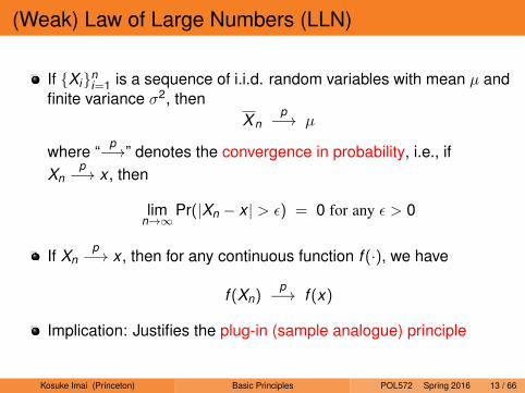
(Weak) Law of Large Numbers (LLN)

If {Xi}ni=1 is a sequence of i.i.d. random variables with mean µ andfinite variance σ2, then

X np−→ µ

where “p−→” denotes the convergence in probability, i.e., if

Xnp−→ x , then

limn→∞

Pr(|Xn − x | > ε) = 0 for any ε > 0

If Xnp−→ x , then for any continuous function f (·), we have

f (Xn)p−→ f (x)

Implication: Justifies the plug-in (sample analogue) principle


LLN in Action

In Journal of Theoretical Biology,1 “Big and Tall Parents have More Sons” (2005)2 “Engineers Have More Sons, Nurses Have More Daughters” (2005)3 “Violent Men Have More Sons” (2006)4 “Beautiful Parents Have More Daughters” (2007)

314 American Scientist, Volume 97 © 2009 Sigma Xi, The Scientific Research Society. Reproduction with permission only. Contact [email protected].

The data are available for download at http://www.stat.columbia.edu/~gelman/research/beautiful/

As of 2007, the 50 most beautiful people of 1995 had 32 girls and 24 boys, or 57.1 percent girls, which is 8.6 percentage points higher than the population frequency of 48.5 percent. This sounds like good news for the hypothesis. But the standard error is 0.5/√(32 + 24) = 6.7 percent, so the discrepancy is not statistically significant. Let’s get more data.

The 50 most beautiful people of 1996 had 45 girls and 35 boys: 56.2 percent girls, or 7.8 percent more than in the general population. Good news! Combining with 1995 yields 56.6 percent girls—8.1 percent more than expected—with a stan-dard error of 4.3 percent, tantaliz-ingly close to statistical significance. Let’s continue to get some confirm-ing evidence.

The 50 most beautiful people of 1997 had 24 girls and 35 boys—no, this goes in the wrong direction, let’s keep going…For 1998, we have 21 girls and 25 boys, for 1999 we have 23 girls and 30 boys, and the class of 2000 has had 29 girls and 25 boys. Putting all the years together and

removing the duplicates, such as Brad Pitt, People’s most beautiful people from 1995 to 2000 have had 157 girls out of 329 children, or 47.7 percent girls (with a standard error of 2.8 percent), a statistically insig-nificant 0.8 percentage points lower than the population frequency. So nothing much seems to be going on here. But if statistically insignificant effects were considered acceptable, we could publish a paper every two years with the data from the latest “most beautiful people.”

Why Is This Important?Why does this matter? Why are we wasting our time on a series of pa-pers with statistical errors that hap-pen not to have been noticed by a journal’s reviewers? We have two reasons: First, as discussed in the next section, the statistical difficul-ties arise more generally with find-ings that are suggestive but not sta-tistically significant. Second, as we discuss presently, the structure of scientific publication and media at-tention seem to have a biasing effect on social science research.

Before reaching Psychology Today and book publication, Kanazawa’s

findings received broad attention in the news media. For example, the popular Freakonomics blog reported,

A new study by Satoshi Kanaza-wa, an evolutionary psychologist at the London School of Econom-ics, suggests . . . there are more beautiful women in the world than there are handsome men. Why? Kanazawa argues it’s be-cause good-looking parents are 36 percent more likely to have a baby daughter as their first child than a baby son—which suggests, evolutionarily speaking, that beauty is a trait more valuable for women than for men. The study was conducted with data from 3,000 Americans, derived from the National Longitudinal Study of Adolescent Health, and was published in the Journal of Theo-retical Biology.

Publication in a peer-reviewed jour-nal seemed to have removed all skepti-cism, which is noteworthy given that the authors of Freakonomics are them-selves well qualified to judge social science research.

In addition, the estimated effect grew during the reporting. As noted above, the 4.7 percent (and not sta-tistically significant) difference in the data became 8 percent in Kanazawa’s choice of the largest comparison (most attractive group versus the average of the four least attractive groups), which then became 26 percent when reported as a logistic regression coefficient, and then jumped to 36 percent for reasons unknown (possibly a typo in a news-paper report). The funny thing is that the reported 36 percent signaled to us right away that something was wrong, since it was 10 to 100 times larger than reported sex-ratio effects in the bio-logical literature. Our reaction when seeing such large estimates was not “Wow, they’ve found something big!” but, rather, “Wow, this study is under-powered!” Statistical power refers to the probability that a study will find a statistically significant effect if one is actually present. For a given true ef-fect size, studies with larger samples have more power. As we have dis-cussed here, “underpowered” studies are unlikely to reach statistical signifi-cance and, perhaps more importantly, they drastically overestimate effect size estimates. Simply put, the noise is stronger than the signal.

1995 1996 1997

1998 1999 2000

32 girls 24 boys

29 girls 25 boys

45 girls 35 boys

21 girls 25 boys

24 girls 35 boys

23 girls 30 boys

Figure 4. The authors performed a sex-ratio study of the offspring of the most beautiful people in the world as selected by People magazine between 1995 and 2000. The girls started strong in 1995 with 32 girls to 24 boys. Girls continued strong in 1996. However, as the sample size grew, the ratio converged on the population frequency, concluding with 157 girls and 172 boys, or 47.7 percent girls, approximately the same as the population frequency of 48.5 percent.

Gelman & Weakliem, American Scientist

Law of Averages in action1 1995: 57.1%2 1996: 56.63 1997: 51.84 1998: 50.65 1999: 49.36 2000: 50.0

No dupilicates: 47.7%

Population frequency: 48.5%


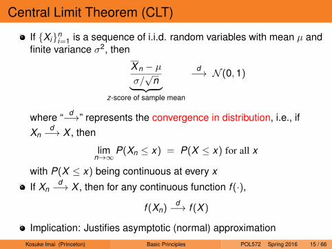
Central Limit Theorem (CLT)

If {Xi}ni=1 is a sequence of i.i.d. random variables with mean µ andfinite variance σ2, then

X n − µσ/√

n︸︷︷︸z-score of sample mean

d−→ N (0,1)

where “ d−→” represents the convergence in distribution, i.e., ifXn

d−→ X , then

limn→∞

P(Xn ≤ x) = P(X ≤ x) for all x

with P(X ≤ x) being continuous at every x

If Xnd−→ X , then for any continuous function f (·),

f (Xn)d−→ f (X )

Implication: Justifies asymptotic (normal) approximationKosuke Imai (Princeton) Basic Principles POL572 Spring 2016 15 / 66

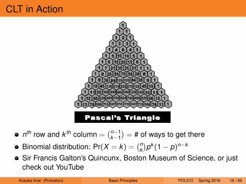
CLT in Action

nth row and k th column =(n−1

k−1

)= # of ways to get there

Binomial distribution: Pr(X = k) =(n

k

)pk (1− p)n−k

Sir Francis Galton’s Quincunx, Boston Museum of Science, or justcheck out YouTube


http://www.youtube.com/watch?v=9xUBhhM4vbM&feature=related

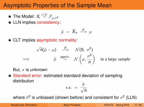
Asymptotic Properties of the Sample Mean

The Model: Xii.i.d.∼ Fµ,σ2

LLN implies consistency:

µ̂ = X np−→ µ

CLT implies asymptotic normality:√

n(µ̂− µ)d−→ N (0, σ2)

=⇒ µ̂approx.∼ N

(µ,σ2

n

)in a large sample

But, σ is unknownStandard error: estimated standard deviation of samplingdistribution

s.e. =σ̂√n

where σ̂2 is unbiased (shown before) and consistent for σ2 (LLN)


Asymptotic Confidence Intervals

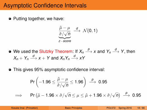
Putting together, we have:

µ̂− µσ̂/√

n︸︷︷︸z−score

d−→ N (0,1)

We used the Slutzky Theorem: If Xnp−→ x and Yn

d−→ Y , thenXn + Yn

d−→ x + Y and XnYnd−→ xY

This gives 95% asymptotic confidence interval:

Pr(−1.96 ≤ µ̂− µ

σ̂/√

n≤ 1.96

)p−→ 0.95

=⇒ Pr(µ̂− 1.96× σ̂/

√n ≤ µ ≤ µ̂+ 1.96× σ̂/

√n) p−→ 0.95


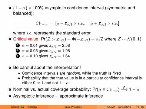
(1− α)× 100% asymptotic confidence interval (symmetric andbalanced):

CI1−α = [µ̂− zα/2 × s.e., µ̂+ zα/2 × s.e.]

where s.e. represents the standard errorCritical value: Pr(Z > zα/2) = Φ(−zα/2) = α/2 where Z ∼ N (0,1)

1 α = 0.01 gives zα/2 = 2.582 α = 0.05 gives zα/2 = 1.963 α = 0.10 gives zα/2 = 1.64

Be careful about the interpretation!Confidence intervals are random, while the truth is fixedProbability that the true value is in a particular confidence interval iseither 0 or 1 and not 1− α

Nominal vs. actual coverage probability: Pr(µ ∈ CI1−α)p−→ 1− α

Asymptotic inference = approximate inference


Exact Inference with Normally Distributed Data

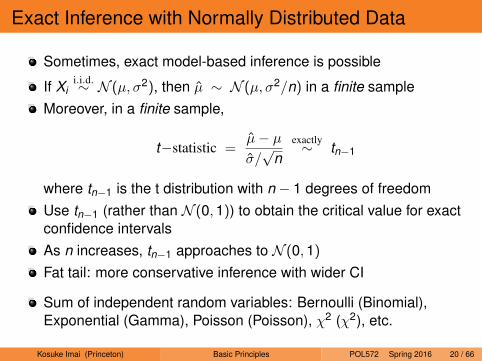
Sometimes, exact model-based inference is possible

If Xii.i.d.∼ N (µ, σ2), then µ̂ ∼ N (µ, σ2/n) in a finite sample

Moreover, in a finite sample,

t−statistic =µ̂− µσ̂/√

nexactly∼ tn−1

where tn−1 is the t distribution with n − 1 degrees of freedomUse tn−1 (rather than N (0,1)) to obtain the critical value for exactconfidence intervalsAs n increases, tn−1 approaches to N (0,1)

Fat tail: more conservative inference with wider CI

Sum of independent random variables: Bernoulli (Binomial),Exponential (Gamma), Poisson (Poisson), χ2 (χ2), etc.


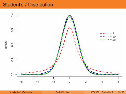
Student’s t Distribution

−6 −4 −2 0 2 4 6

0.0

0.1

0.2

0.3

0.4

dens

ity

n = 2n = 10n = 50


Application: Presidential Election Polling

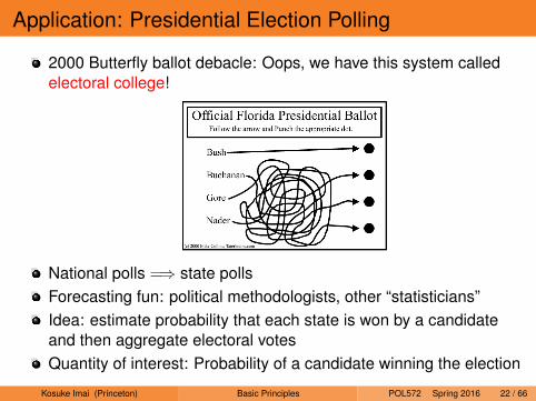
2000 Butterfly ballot debacle: Oops, we have this system calledelectoral college!

National polls =⇒ state pollsForecasting fun: political methodologists, other “statisticians”Idea: estimate probability that each state is won by a candidateand then aggregate electoral votesQuantity of interest: Probability of a candidate winning the election


Simple Model-Based Inference

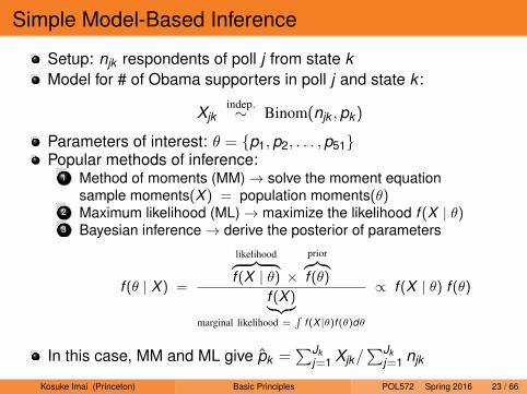
Setup: njk respondents of poll j from state kModel for # of Obama supporters in poll j and state k :

Xjkindep.∼ Binom(njk ,pk )

Parameters of interest: θ = {p1,p2, . . . ,p51}Popular methods of inference:

1 Method of moments (MM)→ solve the moment equationsample moments(X ) = population moments(θ)

2 Maximum likelihood (ML)→ maximize the likelihood f (X | θ)3 Bayesian inference→ derive the posterior of parameters

f (θ | X ) =

likelihood︷︸︸︷f (X | θ) ×

prior︷︸︸︷f (θ)

f (X )︸︷︷︸marginal likelihood =

∫f (X |θ)f (θ)dθ

∝ f (X | θ) f (θ)

In this case, MM and ML give p̂k =∑Jk

j=1 Xjk/∑Jk

j=1 njk


Estimated Probability of Obama Victory in 2008

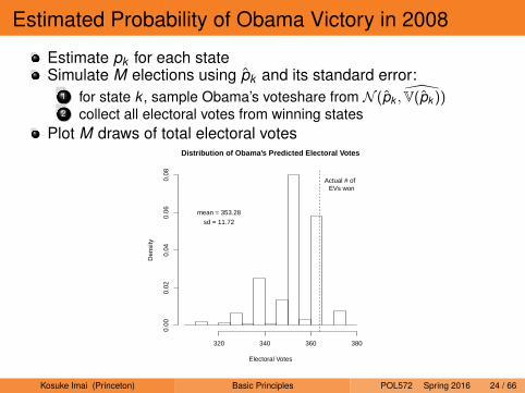
Estimate pk for each stateSimulate M elections using p̂k and its standard error:

1 for state k , sample Obama’s voteshare from N (p̂k , V̂(p̂k ))2 collect all electoral votes from winning states

Plot M draws of total electoral votesDistribution of Obama's Predicted Electoral Votes

Electoral Votes

Den

sity

320 340 360 380

0.00

0.02

0.04

0.06

0.08

Actual # of EVs won

mean = 353.28

sd = 11.72


Nominal vs. Actual Coverage

●

●

●

●

●

●

●

●

●

●

●

●

●

●

●

●

●●●

●●

●

●

●

●

●●

●

●●

●

●

●

●

●

●

●

●

●

●

●●

●

●

●

●

●

●

●

●

●

−20 0 20 40 60 80

−20

020

4060

80

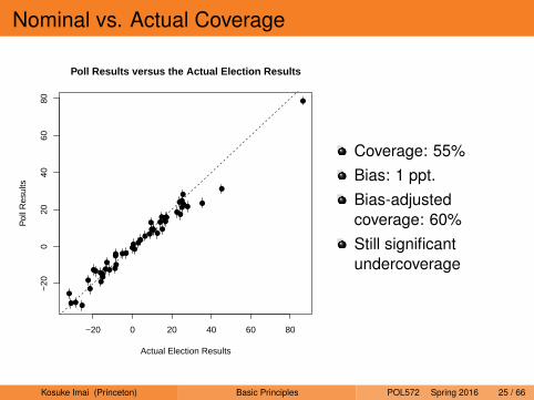
Poll Results versus the Actual Election Results

Actual Election Results

Pol

l Res

ults

Coverage: 55%Bias: 1 ppt.Bias-adjustedcoverage: 60%Still significantundercoverage


Key Points

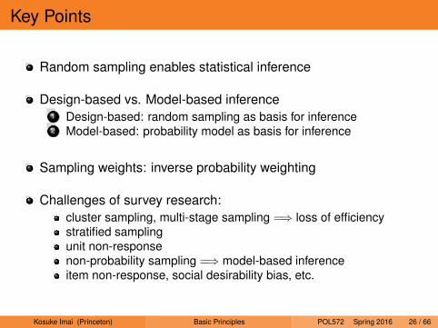
Random sampling enables statistical inference

Design-based vs. Model-based inference1 Design-based: random sampling as basis for inference2 Model-based: probability model as basis for inference

Sampling weights: inverse probability weighting

Challenges of survey research:cluster sampling, multi-stage sampling =⇒ loss of efficiencystratified samplingunit non-responsenon-probability sampling =⇒ model-based inferenceitem non-response, social desirability bias, etc.


Causal Inference


What is Causal Inference?

Comparison between factual and counterfactual for each unit

Incumbency effect:What would have been the election outcome if a candidate werenot an incumbent?

Resource curse thesis:What would have been the GDP growth rate without oil?

Democratic peace theory:Would the two countries have escalated crisis in the samesituation if they were both autocratic?

SUPPLEMENTARY READING: Holland, P. (1986). Statistics andcausal inference. (with discussions) Journal of the AmericanStatistical Association, Vol. 81: 945–960.


http://imai.Princeton.Edu/teaching/files/Cereal.mov

Defining Causal Effects

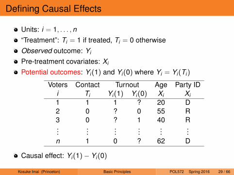
Units: i = 1, . . . ,n“Treatment”: Ti = 1 if treated, Ti = 0 otherwiseObserved outcome: Yi

Pre-treatment covariates: Xi

Potential outcomes: Yi(1) and Yi(0) where Yi = Yi(Ti)

Voters Contact Turnout Age Party IDi Ti Yi(1) Yi(0) Xi Xi1 1 1 ? 20 D2 0 ? 0 55 R3 0 ? 1 40 R...

......

......

...n 1 0 ? 62 D

Causal effect: Yi(1)− Yi(0)


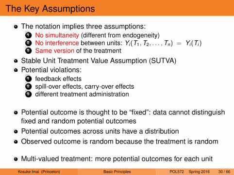
The Key Assumptions

The notation implies three assumptions:1 No simultaneity (different from endogeneity)2 No interference between units: Yi (T1,T2, . . . ,Tn) = Yi (Ti )3 Same version of the treatment

Stable Unit Treatment Value Assumption (SUTVA)Potential violations:

1 feedback effects2 spill-over effects, carry-over effects3 different treatment administration

Potential outcome is thought to be “fixed”: data cannot distinguishfixed and random potential outcomesPotential outcomes across units have a distributionObserved outcome is random because the treatment is random

Multi-valued treatment: more potential outcomes for each unit


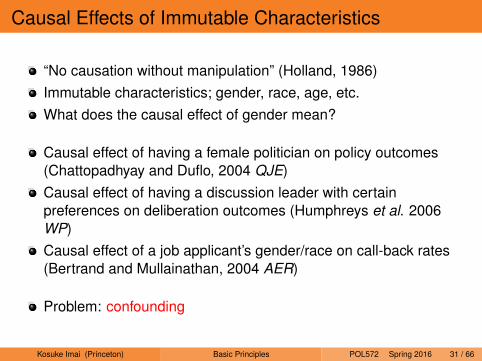
Causal Effects of Immutable Characteristics

“No causation without manipulation” (Holland, 1986)Immutable characteristics; gender, race, age, etc.What does the causal effect of gender mean?

Causal effect of having a female politician on policy outcomes(Chattopadhyay and Duflo, 2004 QJE)Causal effect of having a discussion leader with certainpreferences on deliberation outcomes (Humphreys et al. 2006WP)Causal effect of a job applicant’s gender/race on call-back rates(Bertrand and Mullainathan, 2004 AER)

Problem: confounding


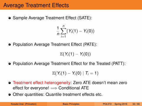
Average Treatment Effects

Sample Average Treatment Effect (SATE):

1n

n∑i=1

(Yi(1)− Yi(0))

Population Average Treatment Effect (PATE):

E(Yi(1)− Yi(0))

Population Average Treatment Effect for the Treated (PATT):

E(Yi(1)− Yi(0) | Ti = 1)

Treatment effect heterogeneity: Zero ATE doesn’t mean zeroeffect for everyone! =⇒ Conditional ATEOther quantities: Quantile treatment effects etc.


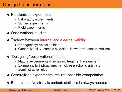
Design Considerations

Randomized experimentsLaboratory experimentsSurvey experimentsField experiments

Observational studies

Tradeoff between internal and external validityEndogeneity: selection biasGeneralizability: sample selection, Hawthorne effects, realism

“Designing” observational studiesNatural experiments (haphazard treatment assignment)Examples: birthdays, weather, close elections, arbitraryadministrative rules

Generalizing experimental results: possible extrapolation

Bottom line: No study is perfect, statistics is always needed


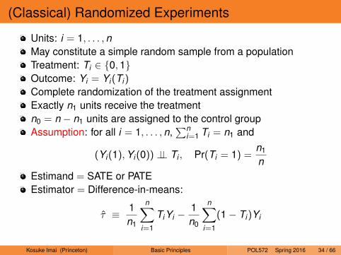
(Classical) Randomized Experiments

Units: i = 1, . . . ,nMay constitute a simple random sample from a populationTreatment: Ti ∈ {0,1}Outcome: Yi = Yi(Ti)

Complete randomization of the treatment assignmentExactly n1 units receive the treatmentn0 = n − n1 units are assigned to the control groupAssumption: for all i = 1, . . . ,n,

∑ni=1 Ti = n1 and

(Yi(1),Yi(0)) ⊥⊥ Ti , Pr(Ti = 1) =n1

nEstimand = SATE or PATEEstimator = Difference-in-means:

τ̂ ≡ 1n1

n∑i=1

TiYi −1n0

n∑i=1

(1− Ti)Yi


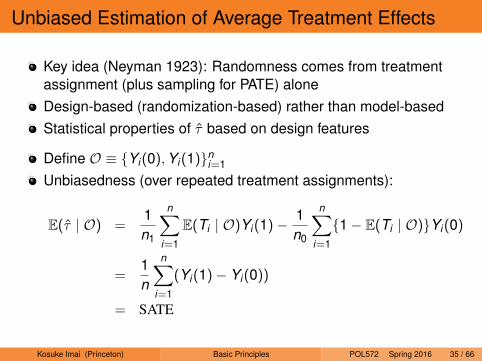
Unbiased Estimation of Average Treatment Effects

Key idea (Neyman 1923): Randomness comes from treatmentassignment (plus sampling for PATE) aloneDesign-based (randomization-based) rather than model-basedStatistical properties of τ̂ based on design features

Define O ≡ {Yi(0),Yi(1)}ni=1

Unbiasedness (over repeated treatment assignments):

E(τ̂ | O) =1n1

n∑i=1

E(Ti | O)Yi(1)− 1n0

n∑i=1

{1− E(Ti | O)}Yi(0)

=1n

n∑i=1

(Yi(1)− Yi(0))

= SATE


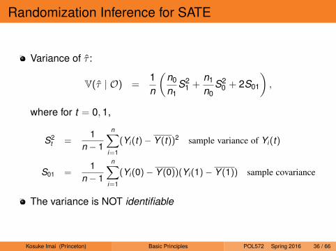
Randomization Inference for SATE

Variance of τ̂ :

V(τ̂ | O) =1n

(n0

n1S2

1 +n1

n0S2

0 + 2S01

),

where for t = 0,1,

S2t =

1n − 1

n∑i=1

(Yi (t)− Y (t))2 sample variance of Yi (t)

S01 =1

n − 1

n∑i=1

(Yi (0)− Y (0))(Yi (1)− Y (1)) sample covariance

The variance is NOT identifiable


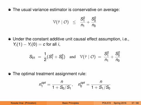
The usual variance estimator is conservative on average:

V(τ̂ | O) ≤S2

1n1

+S2

0n0

Under the constant additive unit causal effect assumption, i.e.,Yi(1)− Yi(0) = c for all i ,

S01 =12

(S21 + S2

0) and V(τ̂ | O) =S2

1n1

+S2

0n0

The optimal treatment assignment rule:

nopt1 =

n1 + S0/S1

, nopt0 =

n1 + S1/S0


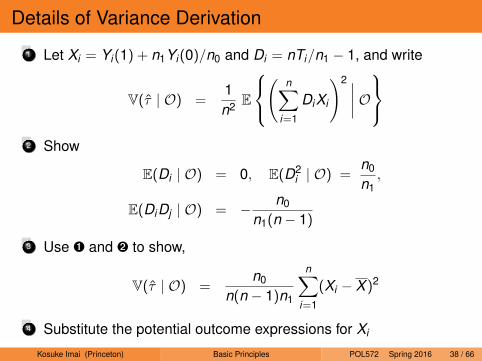
Details of Variance Derivation

1 Let Xi = Yi(1) + n1Yi(0)/n0 and Di = nTi/n1 − 1, and write

V(τ̂ | O) =1n2 E

(

n∑i=1

DiXi

)2 ∣∣∣∣ O

2 Show

E(Di | O) = 0, E(D2i | O) =

n0

n1,

E(DiDj | O) = − n0

n1(n − 1)

3 Use Ê and Ë to show,

V(τ̂ | O) =n0

n(n − 1)n1

n∑i=1

(Xi − X )2

4 Substitute the potential outcome expressions for Xi


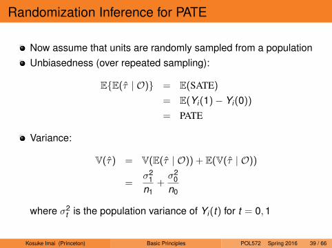
Randomization Inference for PATE

Now assume that units are randomly sampled from a populationUnbiasedness (over repeated sampling):

E{E(τ̂ | O)} = E(SATE)

= E(Yi(1)− Yi(0))

= PATE

Variance:

V(τ̂) = V(E(τ̂ | O)) + E(V(τ̂ | O))

=σ2

1n1

+σ2

0n0

where σ2t is the population variance of Yi(t) for t = 0,1


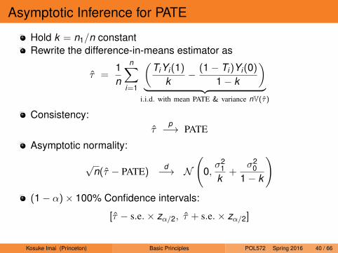
Asymptotic Inference for PATE

Hold k = n1/n constantRewrite the difference-in-means estimator as

τ̂ =1n

n∑i=1

(TiYi(1)

k− (1− Ti)Yi(0)

1− k

)︸︷︷︸

i.i.d. with mean PATE & variance nV(τ̂)

Consistency:τ̂

p−→ PATE

Asymptotic normality:

√n(τ̂ − PATE)

d−→ N

(0,σ2

1k

+σ2

01− k

)(1− α)× 100% Confidence intervals:

[τ̂ − s.e.× zα/2, τ̂ + s.e.× zα/2]


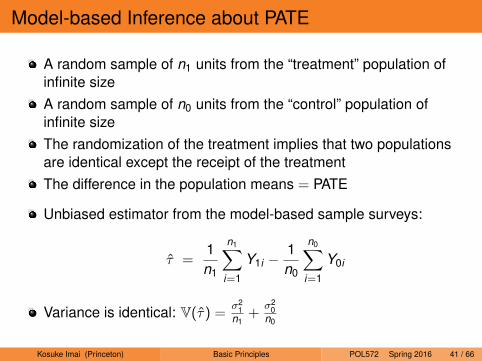
Model-based Inference about PATE

A random sample of n1 units from the “treatment” population ofinfinite sizeA random sample of n0 units from the “control” population ofinfinite sizeThe randomization of the treatment implies that two populationsare identical except the receipt of the treatmentThe difference in the population means = PATE

Unbiased estimator from the model-based sample surveys:

τ̂ =1n1

n1∑i=1

Y1i −1n0

n0∑i=1

Y0i

Variance is identical: V(τ̂) =σ2

1n1

+σ2

0n0


Identification vs. Estimation

Observational studies =⇒ No randomization of treatmentDifference in means between two populations can still beestimated without biasValid inference for ATE requires additional assumptionsLaw of Decreasing Credibility (Manski): The credibility of inferencedecreases with the strength of the assumptions maintained

Identification: How much can you learn about the estimand if youhad an infinite amount of data?Estimation: How much can you learn about the estimand from afinite sample?Identification precedes estimation


Identification of the Average Treatment Effect

Assumption 1: Overlap (i.e., no extrapolation)

0 < Pr(Ti = 1 | Xi = x) < 1 for any x ∈ X

Assumption 2: Ignorability (exogeneity, unconfoundedness, noomitted variable, selection on observables, etc.)

{Yi(1),Yi(0)} ⊥⊥ Ti | Xi = x for any x ∈ X

Under these assumptions, we have nonparametric identification:

τ = E{µ(1,Xi)− µ(0,Xi)}

where µ(t , x) = E(Yi | Ti = t ,Xi = x)


Partial Identification

Partial (sharp bounds) vs. Point identification (point estimates):1 What can be learned without any assumption other than the ones

which we know are satisfied by the research design?2 What is a minimum set of assumptions required for point

identification?3 Can we characterize identification region if we relax some or all of

these assumptions?

ATE with binary outcome:

[−Pr(Yi = 0 | Ti = 1,Xi = x)π(x)− Pr(Yi = 1 | Ti = 0,Xi = x){1− π(x)},Pr(Yi = 1 | Ti = 1,Xi = x)π(x) + Pr(Yi = 0 | Ti = 0,Xi = x){1− π(x)}]

where π(x) = Pr(Ti = 1 | Xi = x) is called propensity score

The width of the bounds is 1: “A glass is half empty/full”


Application: List Experiment

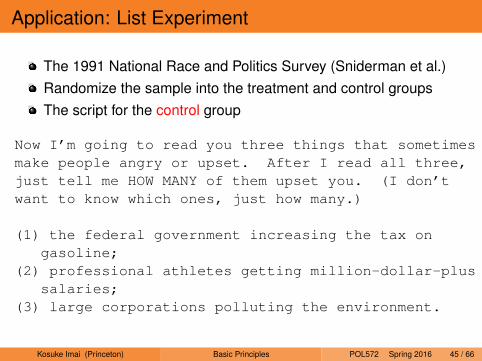
The 1991 National Race and Politics Survey (Sniderman et al.)Randomize the sample into the treatment and control groupsThe script for the control group

Now I’m going to read you three things that sometimesmake people angry or upset. After I read all three,just tell me HOW MANY of them upset you. (I don’twant to know which ones, just how many.)

(1) the federal government increasing the tax ongasoline;

(2) professional athletes getting million-dollar-plussalaries;

(3) large corporations polluting the environment.


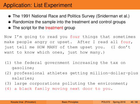
Application: List Experiment

The 1991 National Race and Politics Survey (Sniderman et al.)Randomize the sample into the treatment and control groupsThe script for the treatment group

Now I’m going to read you four things that sometimesmake people angry or upset. After I read all four,just tell me HOW MANY of them upset you. (I don’twant to know which ones, just how many.)

(1) the federal government increasing the tax ongasoline;

(2) professional athletes getting million-dollar-plussalaries;

(3) large corporations polluting the environment;(4) a black family moving next door to you.


Identification Assumptions and Potential Outcomes

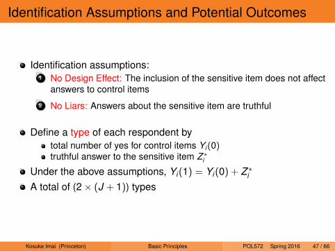
Identification assumptions:1 No Design Effect: The inclusion of the sensitive item does not affect

answers to control items

2 No Liars: Answers about the sensitive item are truthful

Define a type of each respondent bytotal number of yes for control items Yi (0)truthful answer to the sensitive item Z ∗i

Under the above assumptions, Yi(1) = Yi(0) + Z ∗iA total of (2× (J + 1)) types


Example with 3 Control Items

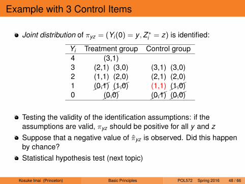
Joint distribution of πyz = (Yi(0) = y ,Z ∗i = z) is identified:

Yi Treatment group Control group4 (3,1)3 (2,1) (3,0) (3,1) (3,0)2 (1,1) (2,0) (2,1) (2,0)1 �

��(0,1) ��(1,0) (1,1) �

��(1,0)0 ��(0,0) ��(0,1) ��(0,0)

Testing the validity of the identification assumptions: if theassumptions are valid, πyz should be positive for all y and zSuppose that a negative value of π̂yz is observed. Did this happenby chance?Statistical hypothesis test (next topic)


Key Points

Causal inference is all about predicting counter-factualsAssociation (comparison between treated and control groups) isnot causation (comparison between factuals and counterfactuals)

Randomization of treatment eliminates both observed andunobserved confoundersDesign-based vs. model-based inference

Observational studies =⇒ identification problemImportance of research design: What is your identificationstrategy?


Statistical Hypothesis Test


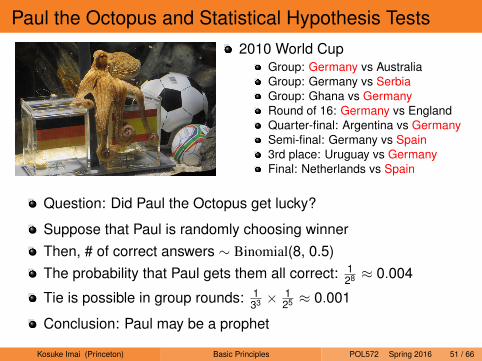
Paul the Octopus and Statistical Hypothesis Tests2010 World Cup

Group: Germany vs AustraliaGroup: Germany vs SerbiaGroup: Ghana vs GermanyRound of 16: Germany vs EnglandQuarter-final: Argentina vs GermanySemi-final: Germany vs Spain3rd place: Uruguay vs GermanyFinal: Netherlands vs Spain

Question: Did Paul the Octopus get lucky?

Suppose that Paul is randomly choosing winnerThen, # of correct answers ∼ Binomial(8, 0.5)The probability that Paul gets them all correct: 1

28 ≈ 0.004

Tie is possible in group rounds: 133 × 1

25 ≈ 0.001

Conclusion: Paul may be a prophet


What are Statistical Hypothesis Tests?

Probabilistic “Proof by contradiction”

General procedure:1 Choose a null hypothesis (H0) and an alternative hypothesis (H1)2 Choose a test statistic Z3 Derive the sampling distribution (or reference distribution) of Z

under H04 Is the observed value of Z likely to occur under H0?

Yes =⇒ Retain H0 (6= accept H0)No =⇒ Reject H0


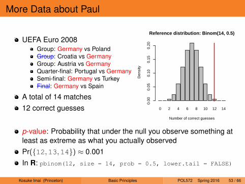
More Data about Paul

UEFA Euro 2008Group: Germany vs PolandGroup: Croatia vs GermanyGroup: Austria vs GermanyQuarter-final: Portugal vs GermanySemi-final: Germany vs TurkeyFinal: Germany vs Spain

A total of 14 matches12 correct guesses 0 2 4 6 8 10 12 14

Reference distribution: Binom(14, 0.5)

Number of correct guesses

Den

sity

0.00

0.05

0.10

0.15

0.20

p-value: Probability that under the null you observe something atleast as extreme as what you actually observedPr({12,13,14}) ≈ 0.001In R: pbinom(12, size = 14, prob = 0.5, lower.tail = FALSE)


p-value and Statistical Significance

p-value: the probability, computed under H0, of observing a valueof the test statistic at least as extreme as its observed valueA smaller p-value presents stronger evidence against H0

p-value less than α indicates statistical significance at thesignificance level α

p-value is NOT the probability that H0 (H1) is true (false)A large p-value can occur either because H0 is true or because H0is false but the test is not powerfulThe statistical significance indicated by the p-value does notnecessarily imply scientific significance

Inverting the hypothesis test to obtain confidence intervalsTypically better to present confidence intervals than p-values


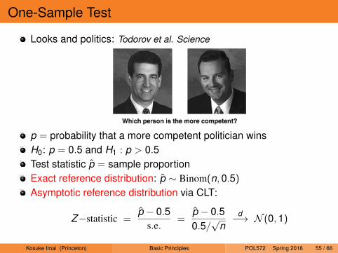
One-Sample Test

Looks and politics: Todorov et al. Science

p = probability that a more competent politician winsH0: p = 0.5 and H1 : p > 0.5Test statistic p̂ = sample proportionExact reference distribution: p̂ ∼ Binom(n,0.5)

Asymptotic reference distribution via CLT:

Z−statistic =p̂ − 0.5

s.e.=

p̂ − 0.50.5/√

nd−→ N (0,1)


Two-Sample Test

H0 : PATE = τ0 and H1 : PATE 6= τ0

Difference-in-means estimator: τ̂Asymptotic reference distribution:

Z−statistic =τ̂ − τ0

s.e.=

τ̂ − τ0√σ̂2

1n1

+σ̂2

0n0

d−→ N (0,1)

Is Zobs unusual under the null?Reject the null when |Zobs| > z1−α/2Retain the null when |Zobs| ≤ z1−α/2

If we assume Yi(1)i.i.d.∼ N (µ1, σ

21) and Yi(0)

i.i.d.∼ N (µ0, σ20), then

t−statistic =τ̂ − τ0

s.e.∼ tν

where ν is given by a complex formula (Behrens-Fisher problem)


Lady Tasting Tea

Does tea taste different depending on whether the tea was pouredinto the milk or whether the milk was poured into the tea?8 cups; n = 8Randomly choose 4 cups into which pour the tea first (Ti = 1)Null hypothesis: the lady cannot tell the differenceSharp null – H0 : Yi(1) = Yi(0) for all i = 1, . . . ,8Statistic: the number of correctly classified cupsThe lady classified all 8 cups correctly!Did this happen by chance?

Example: Ho and Imai (2006). “Randomization Inference withNatural Experiments: An Analysis of Ballot Effects in the 2003California Recall Election.” J. of the Amer. Stat. Assoc.


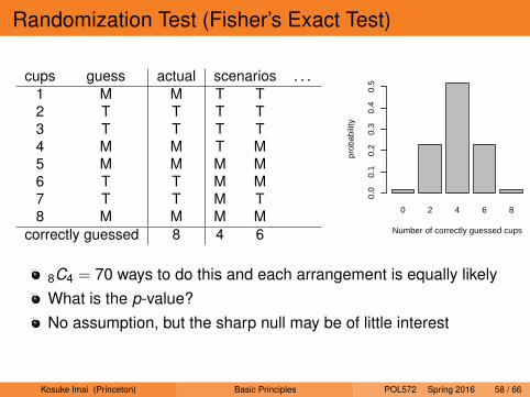
Randomization Test (Fisher’s Exact Test)

cups guess actual scenarios . . .1 M M T T2 T T T T3 T T T T4 M M T M5 M M M M6 T T M M7 T T M T8 M M M M

correctly guessed 8 4 6

0 2 4 6 8

Frequency Plot

Number of correctly guessed cups

freq

uenc

y

05

1020

30

0 2 4 6 8

Probability Distribution

Number of correctly guessed cups

prob

abili

ty

0.0

0.1

0.2

0.3

0.4

0.5

8C4 = 70 ways to do this and each arrangement is equally likelyWhat is the p-value?No assumption, but the sharp null may be of little interest


Error and Power of Hypothesis Test

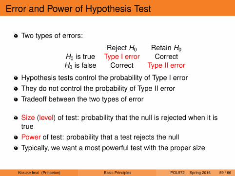
Two types of errors:

Reject H0 Retain H0H0 is true Type I error CorrectH0 is false Correct Type II error

Hypothesis tests control the probability of Type I errorThey do not control the probability of Type II errorTradeoff between the two types of error

Size (level) of test: probability that the null is rejected when it istruePower of test: probability that a test rejects the nullTypically, we want a most powerful test with the proper size


Power Analysis

Null hypotheses are often uninterestingBut, hypothesis testing may indicate the strength of evidence foror against your theoryPower analysis: What sample size do I need in order to detect acertain departure from the null?Power = 1− Pr(Type II error)

Four steps:1 Specify the null hypothesis to be tested and the significance level α2 Choose a true value for the parameter of interest and derive the

sampling distribution of test statistic3 Calculate the probability of rejecting the null hypothesis under this

sampling distribution4 Find the smallest sample size such that this rejection probability

equals a prespecified level


One-Sided Test Example

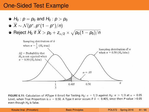
H0 : p = p0 and H0 : p > p0

X ∼ N (p∗,p∗(1− p∗)/n)

Reject H0 if X > p0 + zα/2 ×√

p0(1− p0)/n


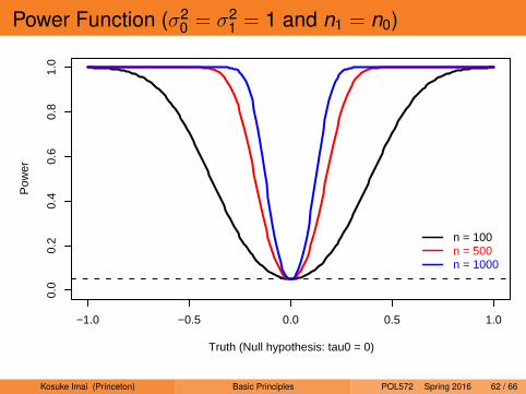
Power Function (σ20 = σ2

1 = 1 and n1 = n0)

−1.0 −0.5 0.0 0.5 1.0

0.0

0.2

0.4

0.6

0.8

1.0

Truth (Null hypothesis: tau0 = 0)

Pow

er

n = 100n = 500n = 1000


Paul’s Rival, Mani the Parakeet

2010 World CupQuarter-final: Netherlands vs BrazilQuarter-final: Uruguay vs GhanaQuarter-final: Argentina vs GermanyQuarter-final: Paraguay vs SpainSemi-final: Uruguay vs NetherlandsSemi-final: Germany vs SpainFinal: Netherlands vs Spain

Mani did pretty good too: p-value is 0.0625

Danger of multiple testing =⇒ false discoveryTake 10 animals with no forecasting ability. What is the chance ofgetting p-value less than 0.05 at least once?

1− 0.9510 ≈ 0.4

If you do this with enough animals, you will find another Paul


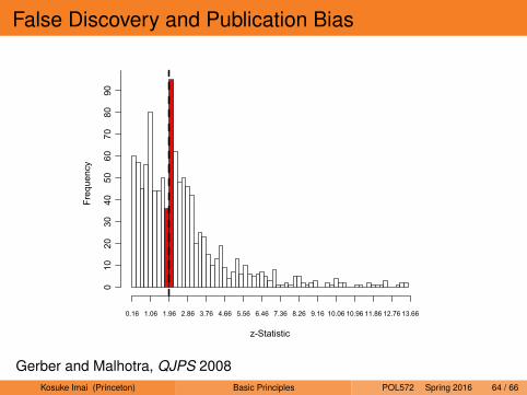
False Discovery and Publication Bias

Do Statistical Reporting Standards Affect What Is Published? 317

including all specifications (full and partial) in the data analysis. We present an exampleof how regression coefficients were selected in the appendix.

RESULTS

Figures 1(b)(a) and 1(b)(b) show the distribution of z-scores7 for coefficients reportedin the APSR and the AJPS for one- and two-tailed tests, respectively.8 The dashed linerepresents the critical value for the canonical 5% test of statistical significance. There isa clear pattern in these figures. Turning first to the two-tailed tests, there is a dramaticspike in the number of z-scores in the APSR and AJPS just over the critical value of 1.96(see Figure 1(b)(a)). The formation in the neighborhood of the critical value resembles

z-Statistic

Fre

qu

en

cy

0.16 1.06 1.96 2.86 3.76 4.66 5.56 6.46 7.36 8.26 9.16 10.06 10.96 11.86 12.76 13.66

01

02

030

40

50

60

70

80

90

Figure 1(a). Histogram of z-statistics, APSR & AJPS (Two-Tailed). Width of bars(0.20) approximately represents 10% caliper. Dotted line represents critical z-statistic(1.96) associated with p = 0.05 significance level for one-tailed tests.

7 The formal derivation of the caliper test is based on z-scores. However, we replicated the analysesusing t-statistics, and unsurprisingly, the results were nearly identical. Generally, studies employedsufficiently large samples, and there were very few coefficients in the extremely narrow caliperbetween 1.96 and 1.99.

8 Very large outlier z-scores are omitted to make the x-axis labels readable. The omitted cases area very small percentage (between 2.4% and 3.3%) of the sample and do not affect the calipertests. Additionally, authors make it clear in tables whether they are testing one-sided or two-sidedhypotheses.

Gerber and Malhotra, QJPS 2008Kosuke Imai (Princeton) Basic Principles POL572 Spring 2016 64 / 66

Statistical Control of False Discovery

Pre-registration system: reduces dishonesty but cannot eliminatemultiple testing problemFamily-wise error rate (FWER): Pr(making at least one Type I error)Bonferroni procedure: reject the j th null hypothesis Hj if pj <

αm

where m is the total number of testsVery conservative: some improvements by Holm and Hochberg

False discovery rate (FDR):

E{

# of false rejectionsmax(total # of rejections,1)

}Adaptive: # of false positives relative to the total # of rejectionsBenjamini-Hochberg procedure:

1 Order p-values p(1) ≤ p(2) ≤ · · · ≤ p(m)

2 Find the largest i such that p(i) ≤ αi/m and call it k3 Reject all H(i) for i = 1,2, . . . , k


Key Points

Stochastic proof by contradiction1 Assume what you want to disprove (null hypothesis)2 Derive the reference distribution of test statistic3 Compare the observed value with the reference distribution

Interpretation of hypothesis test1 Statistical significance 6= scientific significance2 Pay attention to effect size

Power analysis1 Failure to reject null 6= null is true2 Power analysis essential at a planning stage

Danger of multiple testing1 Family-wise error rate, false discovery rate2 Statistical control of false discovery


Basic Principles of Statistical Inference · Probability theory used to model stochastic events...

Documents

Transcript of Basic Principles of Statistical Inference · Probability theory used to model stochastic events...