Basic Principles of Asset Pricing Theory: Evidence from...

Basic Principles of Asset Pricing Theory: Evidence

from Large-Scale Experimental Financial

Markets?

PETER BOSSAERTS1 and CHARLES PLOTT2

1California Institute of Technology and CEPR; 2California Institute of Technology

Abstract. We report on two sets of large-scale financial markets experiments that weredesigned to test the central proposition of modern asset pricing theory, namely, that risk

premia are solely determined by covariance with aggregate risk. We analyze the pricing withinthe framework suggested by two theoretical models, namely, the (general) Arrow and Deb-reu’s complete-markets model, and the (more specific) Sharpe-Lintner-Mossin Capital AssetPricing Model (CAPM). Completeness of the asset payoff structure justifies the former; the

small (albeit non-negligible) risks justifies the latter. We observe swift convergence towardsprice patterns predicted in the Arrow and Debreu and CAPM models. This observation issignificant, because subjects always lack the information to deliberately set asset prices using

either model. In the first set of experiments, however, equilibration is not always robust, withmarkets temporarily veering away. We conjecture that this reflects our failure to controlsubjects’ beliefs about the temporal independence of the payouts. Confirming this conjecture,

the anomaly disappears in a second set of experiments, where states were drawn withoutreplacement. We formally test whether CAPM and Arrow–Debreu equilibrium can be used topredict price movements in our experiments and confirm the hypothesis. When multiplying the

subject payout tenfold (in real terms), to US $ 500 on average for a 3-h experiment, the resultsare unaltered, except for an increase in the recorded risk premia.

? Financial support was provided by the Caltech Laboratory of Experimental Economics and

Political Science, the National Science Foundation, the International Center For Finance at Yale

University and a grant from the Jenkins Family Foundation to Caltech. We thank Bill Brown

(Claremont), Peter DeMarzo (Berkeley, now at Stanford), Will Goetzmann (Yale), Mark Johnson

(Tulane), Tony Kwasnica (Penn State), Claude Montmarquette and Claudia Keser (CIRANO,

Montreal), William Sharpe (Stanford), Woody Studenmund (Occidental College), and Ivo Welch

(UCLA, now at Yale), for allowing us to involve their students in our experimental financial

markets. Elena Asparouhova (now at Utah) facilitated the Bulgarian experiment. The paper bene-

fited from comments at many seminars and meetings throughout the world. Constructive criticism

from the editor and two referees is gratefully accepted, but only the authors are responsible for

remaining errors. Correspondence to: [email protected], [email protected].

135Review of Finance 8: 135–169, 2004.

� 2004 Kluwer Academic Publishers. Printed in the Netherlands.

at University of U

tah on July 9, 2012http://rof.oxfordjournals.org/

Dow

nloaded from

http://rof.oxfordjournals.org/

1. Motivation

Since the early 1950s, two major considerations have driven the develop-ment of asset pricing theory, namely, (i) the presence of risk-averse inves-tors, and (ii) asymmetric information. The former consideration has led toa better theoretical understanding of risk and its equilibrium compensation.The predictions from specific versions of the theory are widely applied inpractical areas, such as capital budgeting and portfolio performance eval-uation, yet empirical support from econometric analysis of historical datahas been dubious at best. The disconnect between theory and empiricalsupport calls for an experimental investigation, which allows for bettercontrol of many of the key assumptions. Asymmetric information addscomplexity to an already controversial theory. Also, with few exceptions(e.g., Biais, et al. 2003), the literature on competitive asset pricing underasymmetric information is entirely theoretical. (There is a large literature ofpricing under asymmetric information in a strategic setting, though.)Therefore, we decided to avoid asymmetric information in the first stage ofour experimental investigation.

The premises of standard asset pricing theory have been that ex-pected utility maximizing agents meet in competitive markets, and thatprices react, to eventually reach general equilibrium. The main impli-cations have been that equilibrium prices will only reflect compensationfor aggregate, i.e., non-diversifiable, risk, and that this risk is to bemeasured in terms of the covariance between the return on a securityand some aggregate risk factor(s). Preferably, the latter can be iden-tified in terms of the return on a specific (set of) benchmark portfo-lio(s).

While competitive market models are a fiction, they are capable of makingaccurate predictions in the laboratory if one uses the right trading interfaceand if a sufficient number of subjects are present. Several choices are avail-able as far as trading interface is concerned. In our experiments, we use acontinuous, web-based (electronic) open book system similar to the one inplace in many stock markets around the world. In such a setting, however,earlier experiments (Bossaerts and Plott 2002) did not produce the expectedresult: prices did not converge to equilibrium configurations. Bossaerts andPlott (2002) conjectured that the number of subjects (5–13), while standard inexperimental economics, is insufficient to make markets liquid enough in aportfolio setting.1 Their reasoning was as follows. Asset pricing theorybecomes non-trivial only when there are at least three securities. As part ofportfolio rebalancing, subjects may want to sell one security to buy another

1 Experimentalists consider 8–12 subjects to be sufficient to generate convergence towards

competitive equilibrium in the laboratory. These numbers come from much simpler experi-ments, however, where at most two goods/securities are traded.

136 PETER BOSSAERTS AND CHARLES PLOTT

at University of U


Dow

nloaded from


one. Since all trading takes place through cash (swaps are not possible),subjects may end up with an inferior portfolio if, because of market thinness,they cannot complete portfolio rebalancing before the end of the period.Subjects may therefore refrain from rebalancing. As a result, prices do notconverge to equilibrium. One of the goals of this paper is to verify whetherthis reasoning is correct, by increasing the number of subjects substantially.In our large-scale experiments, the number of subjects varied between 19 and63.2

Asset pricing theory builds on risk aversion. Provided they have smoothexpected utility preferences, subjects should be approximately risk neutralwhen risk is small. Therefore, one wonders whether risk in laboratoryexperiments can be raised enough for significant risk premia to emerge.There is, however, plenty of evidence in the experimental economics liter-ature that significant risk aversion emerges at the levels of uncertaintypresent in our experiment, in the form of low transaction prices relative toexpected payoffs.3 But note that there are other theories besides riskaversion that could explain discounts, such as the endowment effect. Ourstudy casts new light on the origin of the discounts. Asset pricing theorynot only predicts that risk premia will emerge, but also how these are to bedistributed across assets. So, when the cross-section of the discounts be-comes patterned after the theory, as it does in our experiments, thehypothesis that risk aversion is at work gains credibility.

One way to be convinced that the observed discounts are really risk premiais to increase the size of the risk. In one experiment, we effectively increasedrisk (and return) at least 10-fold. Subjects were Bulgarian students and weoffered them nominally what we had been paying North American subjects.Since the standard of living of the Bulgarian students is at most one-tenth thatof the North American students (at the time of the experiment), the real-termcompensation and risk were at least 10 times as high for the Bulgarians.

In field studies, static asset pricing models are often used to interpretsingle-period returns on multi-period securities. Our experiments are closer tothe theory, because our securities are single-period. In particular, ourexperiments are sequences of replications of the same situation; a replicationis referred to as a period. Neither cash nor asset holdings are carried overfrom one period to another. Still, to mitigate risk-loving behavior because oflimited liability (in the worst case, subjects leave the experiment empty-handed), we introduced a ‘‘solvency rule.’’ The rule creates subtle links

2 As an alternative, one could explore more sophisticated trading mechanisms, meant toalleviate the portfolio rebalancing problem, such as the combined-value auction systems

discussed in Bossaerts, Fine and Ledyard (2002). The need to increase the number of subjectswhen studying more complicated general equilibrium is not unique to asset pricing. See, e.g.,Noussair, Plott and Riezman (1997).

3 See Holt and Laury (2002) for an extensive investigation of the phenomenon.

137ASSET PRICING THEORY

at University of U


Dow

nloaded from


between periods. It works as follows. Subjects’ earnings cumulate acrossperiods; negative earnings in a period are to be offset with positive earnings inother periods; subjects with negative cumulative earnings for two periods in arow are declared insolvent and barred from trading in future periods. A subjectwho is insolvent foregoes an opportunity to gain in the future. This effectivelyinduces caution in all periods but the last.4 Our solvency rule therefore gen-erates subtle dynamic features not captured by the static asset pricing modelswe use to interpret the data. Still, these dynamic features had no noticeableeffect on pricing: risk premia do not decrease over time. (Nor did they havesignificant effects on choices: end-of-period holdings of the vast majority ofsubjects are rationalizable in terms of a fixed, concave utility function.)

Asset pricing theory makes predictions about equilibrium prices that de-pend on agents’ preferences and beliefs. In the case of the model of Arrowand Debreu, strong ordinal predictions about ratios of state prices overprobabilities obtain irrespective of individual preferences, as long as utility issmooth and beliefs are common. CAPM makes cardinal predictions aboutthe pricing of one portfolio, namely, the market portfolio, but imposesstronger requirements on utility: it is assumed to be quadratic. Smooth utilityis only mildly controversial.5 Even quadratic utility can be justified, at least inour experimental setting, because risk is small, so that quadratic utilityobtains as an approximation of true utility. It may seem that commonality ofbeliefs is a not an issue, given clear instructions that explain how states(which determine payoffs) are drawn. As we shall see, however, prices attimes reflect a disbelief in the temporal independence of the drawing across

4 Consider the penultimate period. If a subject manages to satisfy the solvency rule in thatperiod, she receives securities with which to make money in the last period. To maximize theprobability of receiving these valuable securities, our subject has to minimize the probability of

earning less than is required to satisfy the solvency rule. If the payoff distribution is symmetric,maximizing variance, as a risk-neutral subject would do if the penultimate period were reallythe last one, maximizes this probability instead of minimizing it (matters are more complicatedif the payoff distribution is asymmetric). Consequently, the subject has to balance maximizing

expected payoff in the penultimate period against the probability of being thrown out. Inci-dentally, maximizing payoff variance is wrong for a second reason. The payoff in the penul-timate period indirectly determines the nature of the securities in the last period. Indeed,

because we cannot force subjects to pay for losses, the securities they hold actually form acombination of full-liability securities plus a put option. The put option allows her to walkaway from the experiment if she ends with a negative balance. The strike price of the put

option is determined by the cumulative earnings up to the penultimate period. The higherthese cumulative earnings, the lower the strike price of the put option. To increase the value ofthe put option, our subject has to increase the strike price, and hence, to reduce the chances ofgetting high earnings in the penultimate period. Again, maximizing variance, as a risk-neutral

subject would do if the penultimate period were the last one, is not optimal.5 Recently, asset pricing models have been suggested that build on kinks in the utility

function at endowment. See, e.g., Barberis, Huang and Santos (2001), or Epstein and Zin(2001).


at University of U


Dow

nloaded from


periods. We conjectured that subjects have a natural inclination to betterunderstand (and believe) draws without replacement. To verify this, we ranan additional three experiments where states are drawn without replacement.The latter will be referred to as the second set of experiments, to distinguishthem from the first set, which consists of six experiments where states weredrawn with replacement.

The significance of our experimental results is further enhanced by thefollowing design feature. Subjects knew only their own endowment and notthat of others.6 So, they did not know the aggregate endowment. Yet, to pricesecurities in accordance to the Arrow–Debreu model or to the CAPM, theaggregate endowment has to be known. For instance, the CAPM predictsthat prices will be set such that the market portfolio (i.e., the aggregateportfolio of risky securities) is mean-variance optimal. Subjects did not knowthe market portfolio, and hence, could not use the CAPM to price securities.If CAPM pricing emerges in our experiments, it cannot be attributed tosubjects’ using CAPM to determine offer prices.

We hasten to add that neither the Arrow–Debreu model nor the CAPMrequire agents to know the aggregate endowment for its pricing predictions tobe valid. Prices in both models are Walrasian equilibrium prices: agents seeprices and optimize; the prices are such that their optimal demands equalsupplies. Absent asymmetric information,7 agents need not know anythingabout other agents’ preferences, beliefs, endowments, or even the aggregatesupply of securities (the market portfolio).8

Very little experimental work on symmetric-information static assetpricing has been done. There is an older literature on dynamic asset pricing(bubbles), but risk neutrality is invariably assumed. We know of no work onthe Arrow–Debreu equilibrium. A few studies have focused on the CAPM.Kroll, Levy and Rapaport (1988) mainly looked at individual portfoliochoice (in particular, whether individual holdings could be separated into aposition in the riskfree security and a position in the market portfolio). Levy(1997) studied the CAPM in a repeated call market with 20 securities anddiscovered a significantly positive relationship between mean excess returnand covariance with the market return, providing partial support for the

6 They were not even told how many subjects participated and could not determine thenumber because our experiments were web-based, and therefore, decentralized.

7 Under asymmetric information, knowledge of the aggregate endowment does becomeimportant, at least if one entertains a notion of equilibrium that is different from the Walr-asian equilibrium, such as the rational expectations equilibrium. See, e.g., Biais, Bossaerts andSpatt (2003).

8 From an empirical point of view, however, our experiments provide a solution to the Rollcritique. Roll (1977) questioned tests of the CAPM on field data because the empiricist needs

to observe the market portfolio and cannot substitute even a highly correlated proxy. In theexperiments, we are in control of the market portfolio, and hence, know it.


at University of U


Dow

nloaded from


CAPM. (As mentioned before, the CAPM actually imposes a much strongerrestriction, namely, that this relationship be proportional.) Bossaerts andPlott (2002) discusses results of a set of experiments based on a design that isalmost identical to the one described here. Far fewer subjects participated,however, thus reducing competition and ultimately inhibiting convergence, asdiscussed earlier.

Formal inference is hampered by the absence of a suitable measure ofabsolute distance from equilibrium. It is difficult to determine when marketsare close to equilibrium in a theory that focuses exclusively on equilibrium.As a consequence, our statistical tests will not examine to what extent mar-kets are close to equilibrium at a given point, but, more modestly, whetherone can use equilibrium theory to predict in what direction prices move.

The remainder of this paper is organized as follows. Section 2 describesthe experimental setup. Section 3 spells out the theoretical predictions. Evi-dence is reported in Section 4. Section 5 concludes.

2. Experimental Design

The experiments are organized as follows. Three assets can be traded. Two,labeled Securities A and B, have a risky payoff, determined by the randomdrawing of one of three ‘‘states,’’ referred to as States X, Y and Z. The thirdasset, labeled Note, is riskfree, and, unlike the risky securities, can be soldshort, up to eight units.9 At the beginning of each period, subjects are en-dowed with a certain number of Securities A and B and cash (purchases arepaid for in cash). The Notes are in zero net supply.10

During 15–25 min, subjects can submit limit orders which are posted inelectronic books (one for each security); if a limit order crosses the best orderat the other side of the market, it is automatically converted to a marketorder. Strict price and time priority are adhered to. No hidden limit ordersare permitted. Order submission and trading are anonymous in the sense thatonly abstract IDs (numbers between 100 and 200) are shown; the identitiesbehind IDs are never revealed.

After markets close, a state is drawn and dividends are determineddepending on this state and the final holdings of the securities. Payments aremade after subtracting a fixed amount referred to as ‘‘loan repayment,’’ as

9 In neither the Arrow–Debreu equilibrium nor in the CAPM equilibrium are short-saleconstraints on risky securities binding. However, the ability to short sell the riskfree security ispotentially important.

10 Cash is a means of exchange and an asset alike. Notes are only an asset (i.e., cannot beused to buy other securities). As assets, cash and notes are perfect substitutes. But cashprovides a service (payment) which may cause it to be priced differently, at least temporarily

(as long as it provides a payment service). We elaborate when we discuss the empirical resultslater on.


at University of U


Dow

nloaded from


discussed below. Subsequently, assets are taken away, and a new periodstarts (subjects are given a fresh supply of the risky securities, as well as cash,etc.). Each experiment involved up to eight periods.

Subjects are to pay the experimenter for the securities and cash they aregiven at the beginning of each period. Effectively, this means that theexperimenter gives securities and cash on loan, and hence, the payment isreferred to as ‘‘loan repayment.’’ The loan repayment creates leverage,causing a magnification of the risk involved in the holding of Securities Aand B. It also means that subjects could lose money. A subject is barredfrom further trading if s/he has negative cumulative earnings for more thantwo periods in a row. As mentioned in Section 1, this solvency rule inducesrisk-averse behavior even among risk-neutral subjects, except in the lastperiod.

All accounting is done in terms of a fictitious currency called francs, to beexchanged for dollars at the end of the experiment at a pre-announced ex-change rate. In some experiments, subjects are also given an initial sign-upreward, which is fully exposed to risk (i.e., subjects run the risk of losing theentire sign-up reward during the experiment).

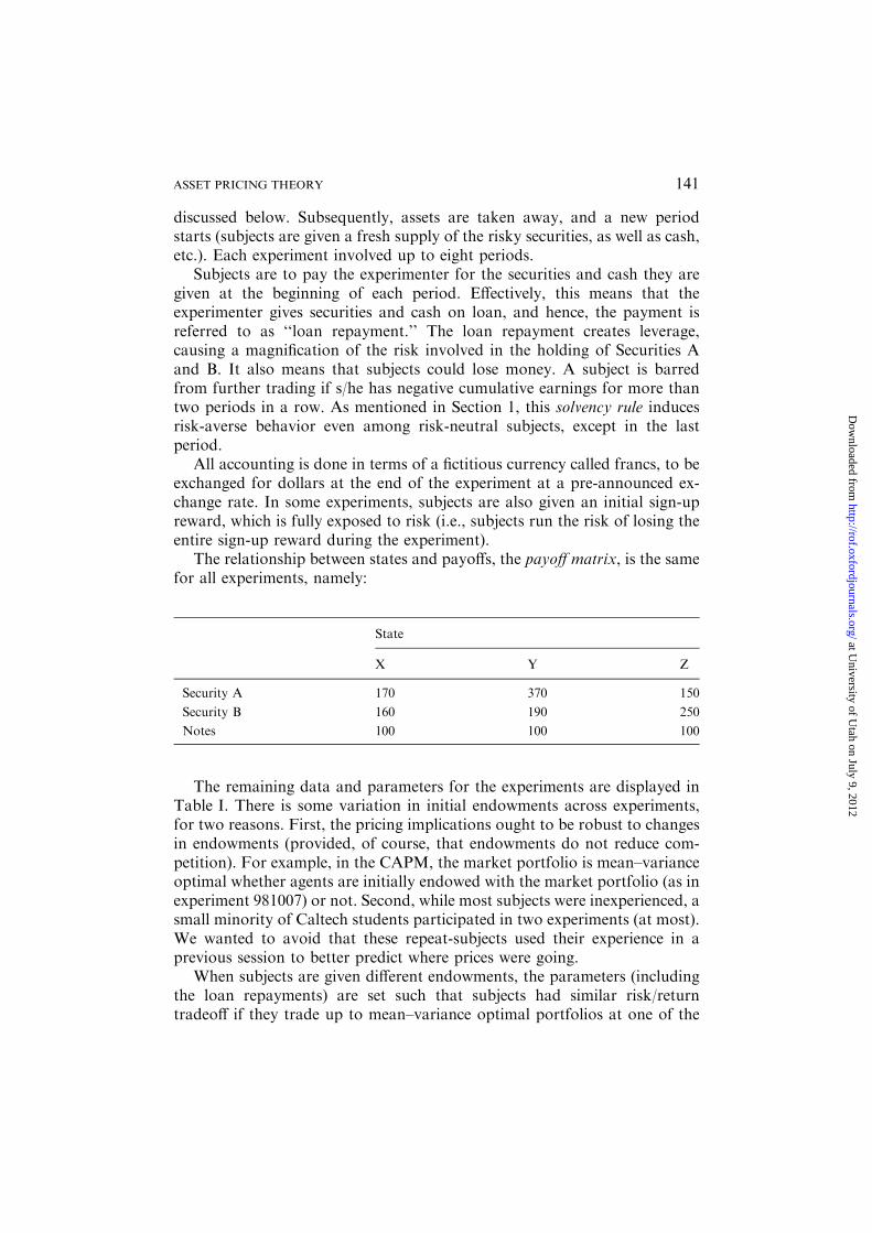
The relationship between states and payoffs, the payoff matrix, is the samefor all experiments, namely:

The remaining data and parameters for the experiments are displayed inTable I. There is some variation in initial endowments across experiments,for two reasons. First, the pricing implications ought to be robust to changesin endowments (provided, of course, that endowments do not reduce com-petition). For example, in the CAPM, the market portfolio is mean–varianceoptimal whether agents are initially endowed with the market portfolio (as inexperiment 981007) or not. Second, while most subjects were inexperienced, asmall minority of Caltech students participated in two experiments (at most).We wanted to avoid that these repeat-subjects used their experience in aprevious session to better predict where prices were going.

When subjects are given different endowments, the parameters (includingthe loan repayments) are set such that subjects had similar risk/returntradeoff if they trade up to mean–variance optimal portfolios at one of the

State

X Y Z

Security A 170 370 150

Security B 160 190 250

Notes 100 100 100


at University of U


Dow

nloaded from


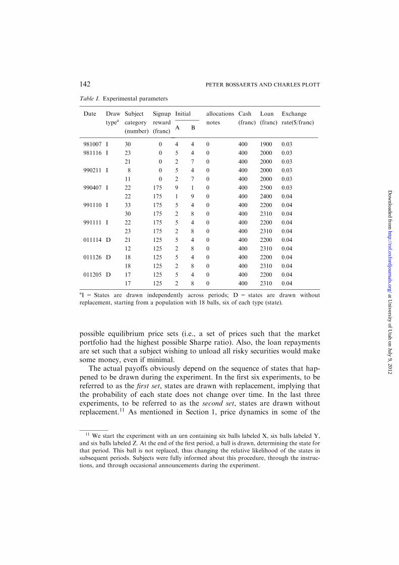
possible equilibrium price sets (i.e., a set of prices such that the marketportfolio had the highest possible Sharpe ratio). Also, the loan repaymentsare set such that a subject wishing to unload all risky securities would makesome money, even if minimal.

The actual payoffs obviously depend on the sequence of states that hap-pened to be drawn during the experiment. In the first six experiments, to bereferred to as the first set, states are drawn with replacement, implying thatthe probability of each state does not change over time. In the last threeexperiments, to be referred to as the second set, states are drawn withoutreplacement.11 As mentioned in Section 1, price dynamics in some of the

Table I. Experimental parameters

Date Draw

typeaSubject

category

(number)

Signup

reward

(franc)

Initial allocations

notes

Cash

(franc)

Loan

(franc)

Exchange

rate($/franc)A B

981007 I 30 0 4 4 0 400 1900 0.03

981116 I 23 0 5 4 0 400 2000 0.03

21 0 2 7 0 400 2000 0.03

990211 I 8 0 5 4 0 400 2000 0.03

11 0 2 7 0 400 2000 0.03

990407 I 22 175 9 1 0 400 2500 0.03

22 175 1 9 0 400 2400 0.04

991110 I 33 175 5 4 0 400 2200 0.04

30 175 2 8 0 400 2310 0.04

991111 I 22 175 5 4 0 400 2200 0.04

23 175 2 8 0 400 2310 0.04

011114 D 21 125 5 4 0 400 2200 0.04

12 125 2 8 0 400 2310 0.04

011126 D 18 125 5 4 0 400 2200 0.04

18 125 2 8 0 400 2310 0.04

011205 D 17 125 5 4 0 400 2200 0.04

17 125 2 8 0 400 2310 0.04

aI = States are drawn independently across periods; D = states are drawn without

replacement, starting from a population with 18 balls, six of each type (state).

11 We start the experiment with an urn containing six balls labeled X, six balls labeled Y,and six balls labeled Z. At the end of the first period, a ball is drawn, determining the state forthat period. This ball is not replaced, thus changing the relative likelihood of the states in

subsequent periods. Subjects were fully informed about this procedure, through the instruc-tions, and through occasional announcements during the experiment.


at University of U


Dow

nloaded from


experiments in the first set (in particular, 990407 and 991111) indicated thatsubjects did not understand or did not believe that states were drawn inde-pendently. Instead, prices behaved as if they believed that the likelihood of astate decreased after it was drawn. To ensure better control of beliefs, wedecided to switch protocols and draw states without replacement in thesecond set of experiments. Note, however, that each period in the second set,markets have to search for an equilibrium with new state probabilities. Thetype of drawing (with, without replacement) for each experiment is indicatedin the second column of Table I.

We had limited control over the number of participants in the experi-ments. Subjects had to register in a database several days before the actualexperiment. After that, they could retrieve an ID and password with which tolog on to the website from which the experiment would be run, and executesome trades as practice. In general, however, subjects were slow to register.Hence, the number of subjects was random. In one experiment, we only had19 subjects (the one referred to as 990211). At the same time, this gives us theopportunity to study the effect of number (of agents) on distance fromequilibrium pricing across experiments.

Subjects are given instructions that they can read on the website beforeeach experiment. The instructions are the same throughout, except for thedescription of the drawing of the states, which is different in the second set ofexperiments. In experiment 011126, subjects were Bulgarian, and a Bulgariantranslation of the instructions was available. (Except for bilingualannouncements, everything during this experiment was in English.)

It should be pointed out that most subjects had familiarity with financialmarkets. This is obvious for MBA students, which constituted the majority ofthe subjects in the first six experiments.12 Caltech students were a minorityfrom the second experiment on, and a majority in the last two experiments.All of them had had exposure to finance and/or micro-economics classes. Anumber of economics students from Claremont and Occidental College, aswell as the University of Montreal also participated in the later experiments.Only Bulgarians from the University of Sofia take part in experiment 011126.Few of these had had prior financial experience.

Average per-subject payments in our experiments is approximately US$50; maximum pay is about US $250 (in experiment 981116, which was a 4-hexperiment, exceptionally); minimum pay is US $0.

The websites for the experiments are as follows:

http://eeps2.caltech.edu/market-981007yale (‘‘981007’’)

12 In 981007 and 990211, students were MBAs from Yale; in 981116, they came from UCLA

(MBAs); in 990407, Stanford MBAs were used; in 991110, Tulane University MBAs partic-ipated; in 991111, the majority of the subjects were Berkeley MBAs.


at University of U


Dow

nloaded from


http://eeps2.caltech.edu/market-981116uclacit (‘‘981116’’)

http://eeps2.caltech.edu/market-990211 (‘‘990211’’)







The interested reader can visit these websites, read the instructions, inspectthe trading interface, and display the trading history (including pricing).13

3. Theoretical Predictions

At the core of modern asset pricing theory is the hypothesis that competitivefinancial markets equilibrate and that, when markets are complete and agentsare expected utility maximizers, equilibrium risk premia can be characterizedin terms of the covariation of an asset’s return with aggregate risk. Completemarkets is the hallmark of the Arrow–Debreu economy: all risks can beinsured. (Debreu, 1959). Such is the case in our experiments. In addition, ourexperiments consist of non-overlapping periods, so we are using a staticmodel to generate pricing predictions.14

Let Ri denote the return (payoff divided by price) on asset i and let u0ðWÞdenote the marginal utility u of wealth W of some ‘‘aggregate’’ investor,which exists by virtue of market completeness. We implicitly take theaggregate investor’s utility to be smooth, so that marginal utilities exist. Weassume that u0ðWÞ is strictly positive (no satiation) and decreasing in wealth(which means that the aggregate investor is risk averse). From the first-orderconditions for optimality of the aggregate investor’s investment–consump-tion plan, it must be that:

E½u0ðWÞRi� ¼ k

13 Anonymous login requires the ID 1 and password a.14 Still, our solvency rule induces subtle dynamic features – but which do not show up in the

pricing, as we report later on.


at University of U


Dow

nloaded from


for some k > 0.15 Let RF denote the return on the riskfree security. The aboverestricts RF as well, so that we can restate the first-order conditions as follows:

E½Ri � RF� ¼ �cov Ri;u0ðWÞ

E½u0ðWÞ�

� �: ð1Þ

The task of asset pricing theory has been to identify the aggregate investor, sothat u0ðWÞ can readily be measured. (Terminal) aggregate wealth equals thepayoff on the aggregate portfolio of all investments in the economy, whichhas become known as the market portfolio.

It deserves emphasis that Equation (1) generates a set of equations thatdefine the Walrasian equilibrium in an Arrow–Debreu world. That is, theyproduce a set of non-linear equations, to be solved for prices. The latter areimplicit in Equation (1). To make them explicit, let Xi denote the payoff onasset i, let Pi denote its price, let PF denote the price of the riskfree security,and assume that the latter’s payoff is 1. Then:

EXi

Pi� 1

PF

� �¼ �cov

Xi

Pi;

u0ðWÞE½u0ðWÞ�

� �: ð2Þ

When markets equilibrate, they effectively solve the set of non-linear equa-tions in (2).

In words, Equation (1) predicts that equilibrium securities prices will besuch that risk premia (expected excess returns) are determined by covariationwith aggregate risk, where aggregate risk is to be measured in terms of themarginal utility of an aggregate investor. This implies not only that riskpremia will exist, but also what their form will be. Let us formally state thefirst part, and then study more closely the second part.

Risk Pricing Property: Risk premia will exist, i.e., equilibrium prices willgenerally deviate from expected payoffs.

The restrictions in Equation (1) describes equilibrium prices in an Arrow–Debreuworldwhere agents have smooth expected utility preferences. They canbe converted in restrictions on the prices of (imaginary) state securities that areeasily verifiable in an experimental setting (where aggregate wealth is ob-servable). To see this, let there be S possible states, indexed s ¼ 1; . . . ;S, eachwith probability ps (

PSi¼1 ps ¼ 1). Let Ps denote the price of state security s

(that is, the security that pays US $1 if state s occurs, and US $ 0 otherwise).Let Ws denote the wealth of the aggregate investor in state s. Re-arrangingEquation (1), one obtains:

15 In the experiments, periods are short, so that we expect k ¼ 1, i.e., the riskfree rate equalszero. We confirm this in the experiments (see the discussion of the empirical results). For the

theory, we will leave k (and the riskfree rate) unspecified, as our arguments do not rely on anyspecific value.


at University of U


Dow

nloaded from


Ps ¼ PFpsu0ðWsÞE½u0ðWÞ� : ð3Þ

Therefore, two states s and s0 with equal likelihood (ps ¼ ps0) have prices thatare ranked solely because of differences in aggregate wealth. If Ws > Ws0 ,then u0ðWsÞ < u0ðWs0 Þ (because of decreasing marginal utility, i.e., riskaversion), and, hence, Ps < Ps0 . The ranking of the state prices is the inverseof the ranking of aggregate consumption (wealth).

When two states have different likelihoods, then the rank order restrictiondoes not apply to state prices, but to the ratio of state prices over proba-bilities, referred to as state price probability ratios, and denoted qs:

qs ¼ Ps=ps: ð4Þ

This observation is the foundation for another theoretical property that wewant to study in experimental markets.

State Price Probability Ratio Property: The ranking of state price proba-bility ratioswill be the inverse of the ranking of aggregatewealth in those states.

The restriction in Equation (3) allows state prices to be above stateprobabilities. That is, (implicit) state securities may trade at a premium toexpected payoff, implying that risk premia may be negative. We verify thisseemingly counter-intuitive implication in the experimental data.

The State Price ProbabilityRatio Property is ordinal. To produce a cardinalprediction, we need to bemore specific about the shape of the utility function ofthe representative agent. We have only been assuming that the utility functionis smooth. Our experimental setting allows us to be more specific. While non-negligible, risk is small. This justifies a quadratic approximation of subjects’actual preferences. Under quadratic preferences, the Capital Asset PricingModel (CAPM, developed in Sharpe 1964; Lintner 1965; Mossin 1966) ob-tains. In other words, the level of risk in our experiments gives the Arrow–Debreu model cardinal content because CAPM pricing will obtain.16

The CAPM predicts that risk premia will be proportional to the covari-ance between a security’s return and the return on a specific benchmark

16 We emphasize that we employ quadratic utility only as a local approximation. As a globaldescription of utility, it is highly unsatisfactory, because it violates the axiom of non-satiationon which the Arrow–Debreu model is built. That is, for sufficiently high wealth levels, subjectsare satiated. As Dybvig and Ingersoll (1982) show, this conflicts with the non-satiation on

which absence of arbitrage is based. In particular, they show that arbitrage opportunitiesbecome possible (if the market portfolio has sufficiently high payoff in some states). Later on,we will demonstrate directly that arbitrage opportunities almost never emerge in our experi-

ments, because state securities prices are always strictly between zero and one and add up toone.


at University of U


Dow

nloaded from


portfolio, namely, the market portfolio (i.e., the value-weighted portfolio ofall risky securities). To see this mathematically, re-consider Equation (1).Utility is quadratic, and, hence, u0ðWÞ ¼ a� bW, for two positive coefficientsa and b. Re-arranging Equation (1), one obtains:

E½Ri � RF� ¼b

E½u0ðWÞ� covðRi;WÞ:

Let PM denote the price of the market portfolio (the aggregate portfolio ofinvestments in the economy). Its payoff, XM, equals W. Let RM denote itsreturn, i.e., XM=PM. For the market portfolio,

E½RM � RF� ¼bPM

E½u0ðWÞ� varðRMÞ:

Using this to solve for b=E½u0ðWÞ�, one obtains:

E½Ri � RF� ¼ covðRi;RMÞE½RM � RF�varðRMÞ : ð5Þ

In words, risk premia are proportional to covariances with the return on themarket portfolio. The constant of proportionality is given by the expectedexcess return on the market portfolio divided by its variance.17

Roll (1977) shows that Equation (5) obtains whenever the market port-folio is mean–variance optimal, i.e., generates maximum expected returngiven its risk (return variance). This means that Equation (5) can be verifiedin a simple way using the Sharpe ratio (reward-to-risk) ratio of the marketportfolio, i.e.,

E½RM � RF�ffiffiffiffiffiffiffiffiffiffiffiffiffiffiffiffiffiffivarðRMÞ

p :

17 Conventionally, the CAPM is re-written as follows:

E½Ri � RF� ¼ biE½RM � RF�;

where

bi ¼covðRi;RMÞvarðRMÞ ;

i.e., the slope coefficient (‘‘beta’’) in an OLS projection of Ri onto RM.


at University of U


Dow

nloaded from


The market portfolio is mean–variance optimal if and only if the market’sSharpe ratio is maximal. Away from the CAPM equilibrium, the market’sSharpe ratio may not be maximal. Hence, the difference between themarket’s Sharpe ratio and the maximal Sharpe ratio provides a simplemeasure of how far the market is from the CAPM equilibrium. Thus,CAPM implies the following property.

Sharpe Ratio Property: The Sharpe ratio of the market will be maximal.Both the State Price Probability Ratio Property and the Sharpe RatioProperty have one important advantage. They provide a description ofmarket equilibrium irrespective of the distribution of risk aversion or initialendowments across investors. Risk aversion and endowments may change(endowments definitely change once subjects trade), and hence, to haveproperties of equilibrium that do not require risk aversion or endowments toremain constant is a definite plus.

4. Results

The evidence on the theoretical properties will be presented here.

4.1. EVIDENCE FOR THE RISK PRICING PROPERTY

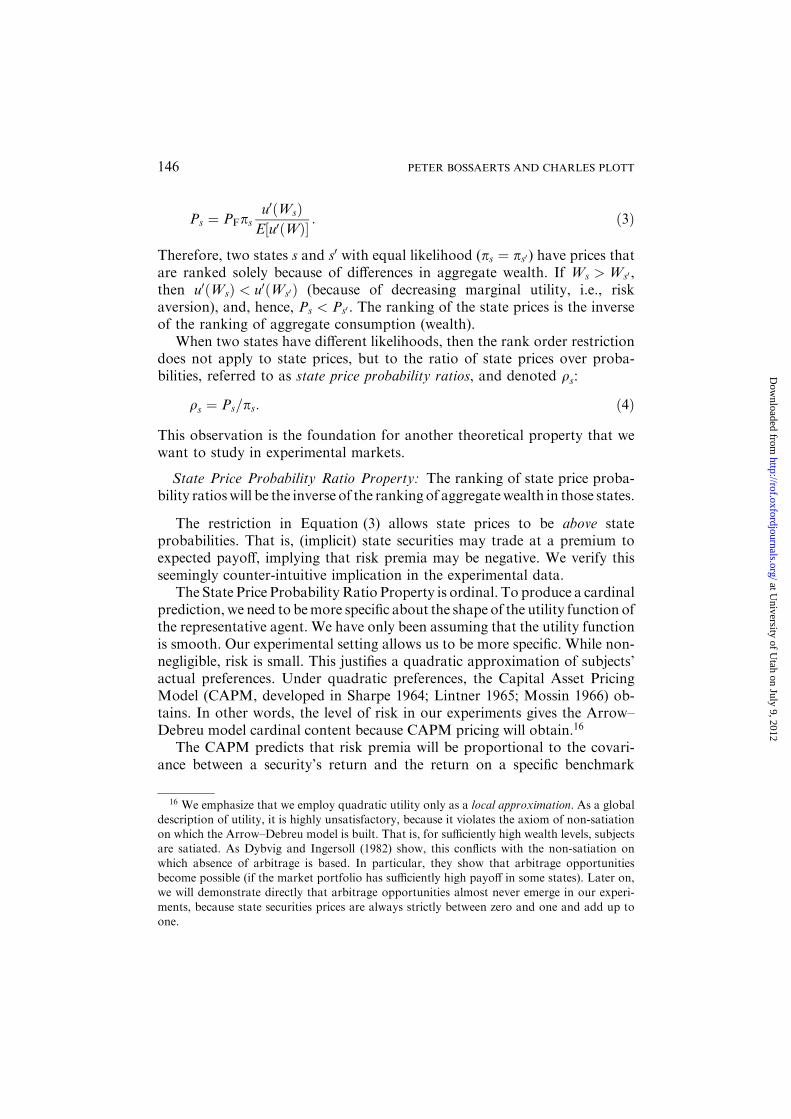
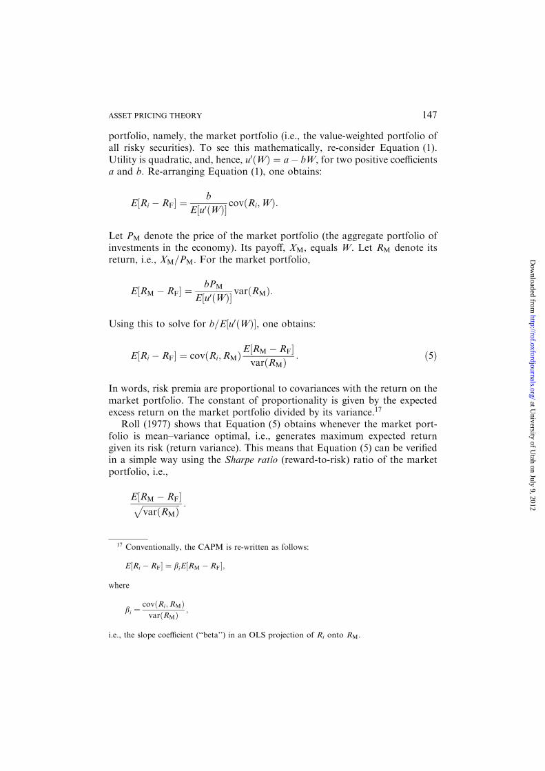
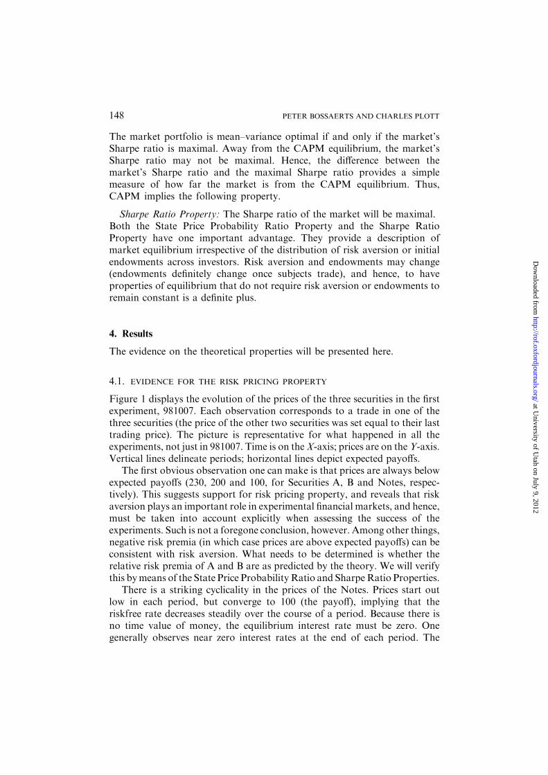
Figure 1 displays the evolution of the prices of the three securities in the firstexperiment, 981007. Each observation corresponds to a trade in one of thethree securities (the price of the other two securities was set equal to their lasttrading price). The picture is representative for what happened in all theexperiments, not just in 981007. Time is on theX-axis; prices are on theY-axis.Vertical lines delineate periods; horizontal lines depict expected payoffs.

The first obvious observation one can make is that prices are always belowexpected payoffs (230, 200 and 100, for Securities A, B and Notes, respec-tively). This suggests support for risk pricing property, and reveals that riskaversion plays an important role in experimental financial markets, and hence,must be taken into account explicitly when assessing the success of theexperiments. Such is not a foregone conclusion, however. Among other things,negative risk premia (in which case prices are above expected payoffs) can beconsistent with risk aversion. What needs to be determined is whether therelative risk premia of A and B are as predicted by the theory. We will verifythis bymeans of the State Price ProbabilityRatio and SharpeRatio Properties.

There is a striking cyclicality in the prices of the Notes. Prices start outlow in each period, but converge to 100 (the payoff), implying that theriskfree rate decreases steadily over the course of a period. Because there isno time value of money, the equilibrium interest rate must be zero. Onegenerally observes near zero interest rates at the end of each period. The


at University of U


Dow

nloaded from


transient positive interest rates reflect subjects’ willingness to borrow inorder to execute the securities trades that are needed to optimize theirportfolio. Because purchases are paid for in cash, and orders in one marketcannot be made conditional on trades in other markets, subjects need tohave a certain amount of cash to execute their purchase orders if they donot wish to sit there and wait for their sales orders for other securities to beexecuted first.

As a matter of fact, monetary theory has appealed to such a cash in advanceconstraints to explain the presence of interest-bearing nominally riskfreesecurities along with zero-interest cash (Clower 1967; Lucas 1982). Monetarytheorists, however, have generally attributed cash-in-advance constraints tothe purchase of consumption goods. In our experiments, they are clearly atwork in investment decisions as well. Our findings would suggest that it maybe worthwhile to study the effect of portfolio re-allocations in explaining thebehavior of interest rates in naturally occurring financial markets as well.

Figure 2 displays the evolution of transaction prices for experiment011126. Remember that Bulgarian subjects were used in this experiment,

0 1000 2000 3000 4000 5000 6000 7000 8000 9000 1000080

100

120

140

160

180

200

220

240

time (in seconds )

Pric

es (

in fr

ancs

)

Security ASecurity BNotes

Figure 1. Evolution of securities prices in the 981007 experiment. Vertical lines delin-eate periods; horizontal lines depict expected payoffs (top line: security A; middle line:

security B; bottom line: Notes). All transactions of risky securities occurred at pricesstrictly below expected payoffs, suggesting risk aversion.


at University of U


Dow

nloaded from


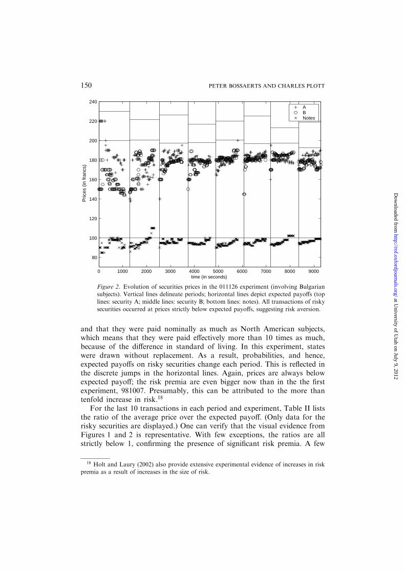
and that they were paid nominally as much as North American subjects,which means that they were paid effectively more than 10 times as much,because of the difference in standard of living. In this experiment, stateswere drawn without replacement. As a result, probabilities, and hence,expected payoffs on risky securities change each period. This is reflected inthe discrete jumps in the horizontal lines. Again, prices are always belowexpected payoff; the risk premia are even bigger now than in the the firstexperiment, 981007. Presumably, this can be attributed to the more thantenfold increase in risk.18

For the last 10 transactions in each period and experiment, Table II liststhe ratio of the average price over the expected payoff. (Only data for therisky securities are displayed.) One can verify that the visual evidence fromFigures 1 and 2 is representative. With few exceptions, the ratios are allstrictly below 1, confirming the presence of significant risk premia. A few

0 1000 2000 3000 4000 5000 6000 7000 8000 9000

80

100

120

140

160

180

200

220

240

time (in seconds)

Pric

es (

in fr

ancs

)

ABNotes

Figure 2. Evolution of securities prices in the 011126 experiment (involving Bulgariansubjects). Vertical lines delineate periods; horizontal lines depict expected payoffs (toplines: security A; middle lines: security B; bottom lines: notes). All transactions of risky

securities occurred at prices strictly below expected payoffs, suggesting risk aversion.

18 Holt and Laury (2002) also provide extensive experimental evidence of increases in riskpremia as a result of increases in the size of risk.


at University of U


Dow

nloaded from


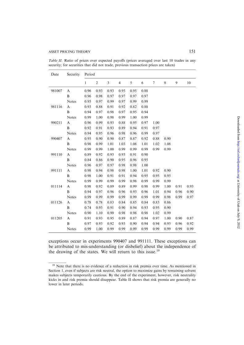
exceptions occur in experiments 990407 and 991111. These exceptions canbe attributed to mis-understanding (or disbelief) about the independence ofthe drawing of the states. We will return to this issue.19

Table II. Ratio of prices over expected payoffs (prices averaged over last 10 trades in anysecurity; for securities that did not trade, previous transaction prices are taken)

Date Security Period

1 2 3 4 5 6 7 8 9 10

981007 A 0.96 0.93 0.93 0.95 0.95 0.88

B 0.96 0.98 0.97 0.97 0.97 0.97

Notes 0.95 0.97 0.99 0.97 0.99 0.99

981116 A 0.93 0.88 0.91 0.92 0.82 0.88

B 0.94 0.97 0.98 0.97 0.95 0.94

Notes 0.99 1.00 0.98 0.99 1.00 0.99

990211 A 0.96 0.99 0.93 0.88 0.95 0.97 1.00

B 0.92 0.91 0.93 0.89 0.94 0.91 0.97

Notes 0.94 0.95 0.96 0.98 0.96 0.99 0.97

990407 A 0.95 0.90 0.90 0.87 0.87 0.92 0.88 0.90

B 0.98 0.99 1.01 1.03 1.08 1.01 1.02 1.08

Notes 0.99 0.99 1.00 0.99 0.99 0.99 0.99 0.99

991110 A 0.89 0.92 0.93 0.93 0.91 0.90

B 0.84 0.86 0.90 0.95 0.96 0.95

Notes 0.96 0.97 0.97 0.98 0.98 1.00

991111 A 0.98 0.94 0.98 0.98 1.00 1.01 0.92 0.90

B 0.98 1.00 0.91 0.91 0.94 0.95 0.95 0.95

Notes 0.99 0.99 0.99 0.99 0.98 0.99 0.99 0.99

011114 A 0.98 0.92 0.89 0.89 0.99 0.98 0.99 1.00 0.91 0.93

B 0.94 0.97 0.96 0.96 0.93 0.96 1.01 0.94 0.96 0.90

Notes 0.99 0.99 0.99 0.99 0.99 0.99 0.99 0.98 0.99 0.97

011126 A 0.78 0.78 0.83 0.84 0.85 0.84 0.83 0.86

B 0.74 0.93 0.91 0.90 0.94 0.93 0.95 0.90

Notes 0.90 1.10 0.99 0.98 0.98 0.98 1.02 0.99

011205 A 0.91 0.93 0.95 0.89 0.87 0.94 0.97 1.00 0.90 0.87

B 0.97 0.93 0.92 0.93 0.90 0.94 0.94 0.95 0.96 0.92

Notes 0.99 1.00 0.99 0.99 0.99 0.99 0.99 0.99 0.99 0.99

19 Note that there is no evidence of a reduction in risk premia over time. As mentioned inSection 1, even if subjects are risk neutral, the option to maximize gains by remaining solventmakes subjects temporarily cautious. By the end of the experiment, however, risk neutrality

kicks in and risk premia should disappear. Table II shows that risk premia are generally nolower in later periods.


at University of U


Dow

nloaded from


4.2. EVIDENCE FOR THE STATE PRICE PROBABILITY RATIO PROPERTY

We deduced state prices for the three states from the transaction prices of thethree securities. As has become standard in mathematical finance andderivatives analysis, we normalized the prices to add up to one. We thendivide the state prices by the probabilities of the states to obtain the stateprice probability ratio. The State Price Probability Ratio Property predictsthat state price probability ratios will be ranked inversely to the aggregatewealth in each state. In all periods of all experiments, initial endowments andpayoffs were such that the aggregate wealth was highest in state Y and lowestin state X. Consequently, state price probability ratios should be lowest in Yand highest in X.

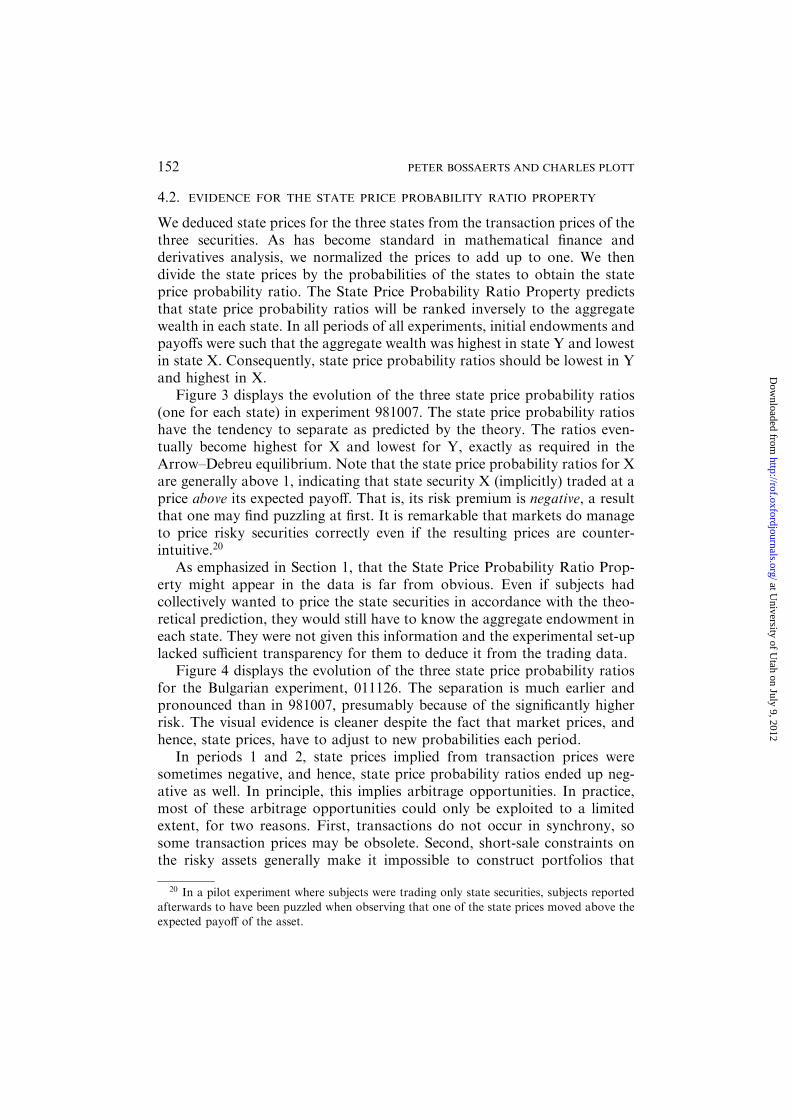
Figure 3 displays the evolution of the three state price probability ratios(one for each state) in experiment 981007. The state price probability ratioshave the tendency to separate as predicted by the theory. The ratios even-tually become highest for X and lowest for Y, exactly as required in theArrow–Debreu equilibrium. Note that the state price probability ratios for Xare generally above 1, indicating that state security X (implicitly) traded at aprice above its expected payoff. That is, its risk premium is negative, a resultthat one may find puzzling at first. It is remarkable that markets do manageto price risky securities correctly even if the resulting prices are counter-intuitive.20

As emphasized in Section 1, that the State Price Probability Ratio Prop-erty might appear in the data is far from obvious. Even if subjects hadcollectively wanted to price the state securities in accordance with the theo-retical prediction, they would still have to know the aggregate endowment ineach state. They were not given this information and the experimental set-uplacked sufficient transparency for them to deduce it from the trading data.

Figure 4 displays the evolution of the three state price probability ratiosfor the Bulgarian experiment, 011126. The separation is much earlier andpronounced than in 981007, presumably because of the significantly higherrisk. The visual evidence is cleaner despite the fact that market prices, andhence, state prices, have to adjust to new probabilities each period.

In periods 1 and 2, state prices implied from transaction prices weresometimes negative, and hence, state price probability ratios ended up neg-ative as well. In principle, this implies arbitrage opportunities. In practice,most of these arbitrage opportunities could only be exploited to a limitedextent, for two reasons. First, transactions do not occur in synchrony, sosome transaction prices may be obsolete. Second, short-sale constraints onthe risky assets generally make it impossible to construct portfolios that

20 In a pilot experiment where subjects were trading only state securities, subjects reported

afterwards to have been puzzled when observing that one of the state prices moved above theexpected payoff of the asset.


at University of U


Dow

nloaded from


mimic the payoff on the state securities, and hence, that exploit the negativeprices.

One would like a formal test to confirm that state price probability ratiostend to move in the direction predicted by the Arrow–Debreu equilibrium.We propose here a test that determines whether state price probability ratiosadjust correctly when their ranking is not as predicted by the theory. We takerandom walk pricing as our null hypothesis. The random walk hypothesis isan appropriate benchmark, because it is devoid of economic content beyondthe statement that it does not allow for either arbitrage opportunities orsimple speculative profit opportunities. Indeed, it is the best model of pricebehavior one had before asset pricing theory was developed. The traditionbehind this model goes back to Bachelier (1900).

Our test calculates the probability of observing the dynamics in state priceprobability ratios actually observed in our experiments if price dynamicswere merely of the random walk type. Under the alternative that markets areattracted by the Arrow–Debreu equilibrium, we expect specific changes in the

0 1000 2000 3000 4000 5000 6000 7000 8000 9000 100000.5

1

1.5

2

time (in seconds)

Sta

te P

rice

Pro

babi

lity

Rat

ios

State XState YState Z

Figure 3. Evolution of ratios of state prices over state probabilities in the 981007experiment. Vertical lines delineate periods. In the Arrow–Debreu equilibrium withexpected utility preferences, the state price probability ratio of X should be highest; thatof Y should be lowest.


at University of U


Dow

nloaded from


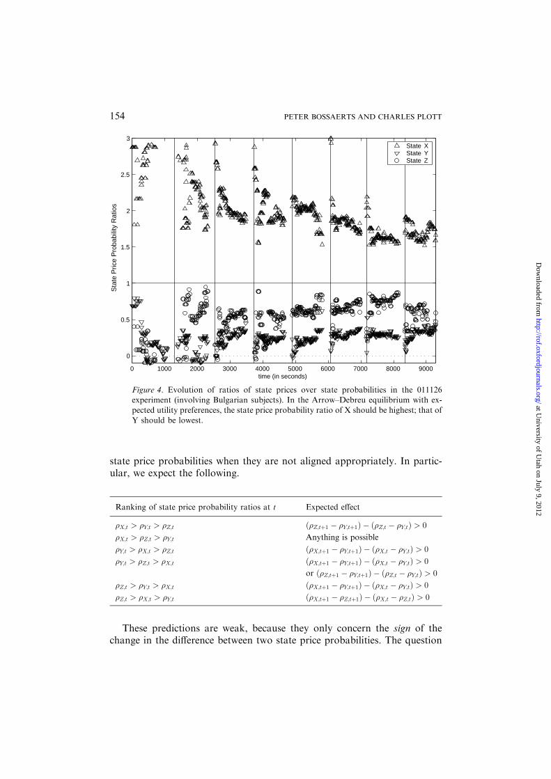
state price probabilities when they are not aligned appropriately. In partic-ular, we expect the following.

These predictions are weak, because they only concern the sign of thechange in the difference between two state price probabilities. The question

0 1000 2000 3000 4000 5000 6000 7000 8000 9000

0

0.5

1

1.5

2

2.5

3

time (in seconds)

Sta

te P

rice

Pro

babi

lity

Rat

ios


Figure 4. Evolution of ratios of state prices over state probabilities in the 011126experiment (involving Bulgarian subjects). In the Arrow–Debreu equilibrium with ex-pected utility preferences, the state price probability ratio of X should be highest; that of

Y should be lowest.

Ranking of state price probability ratios at t Expected effect

�X;t > �Y;t > �Z;t ð�Z;tþ1 � �Y;tþ1Þ � ð�Z;t � �Y;tÞ > 0

�X;t > �Z;t > �Y;t Anything is possible

�Y;t > �X;t > �Z;t ð�X;tþ1 � �Y;tþ1Þ � ð�X;t � �Y;tÞ > 0

�Y;t > �Z;t > �X;t ð�X;tþ1 � �Y;tþ1Þ � ð�X;t � �Y;tÞ > 0

or ð�Z;tþ1 � �Y;tþ1Þ � ð�Z;t � �Y;tÞ > 0

�Z;t > �Y;t > �X;t ð�X;tþ1 � �Y;tþ1Þ � ð�X;t � �Y;tÞ > 0

�Z;t > �X;t > �Y;t ð�X;tþ1 � �Z;tþ1Þ � ð�X;t � �Z;tÞ > 0


at University of U


Dow

nloaded from


is: are economic forces strong enough that the expected effects can bedetected sharply?

As test statistic, we compute the frequency of observing (transisting to) theexpected outcome for each state (ranking of state price probabilities). Wesubsequently take the mean across states. The latter is mandated by the factthat, in finite samples, not all states need occur, in which case some transitionfrequencies are undefined. Notice that the second frequency will always be1.21 We include this frequency, so that outcomes where the Arrow–Debreuprediction holds (qX;t > qZ;t > qY;t) receive more weight. Let s denote thismean transition frequency.

To test whether the observed mean transition frequencies are unusualunder the assumption of a random walk, and hence, to determine whether toreject the null of a random walk, we compute the distribution of s under thenull hypothesis by bootstrapping the empirical joint distribution of pricechanges in each experiment. In the bootstrap, we generated 200 price series ofthe same length as the sample used to estimate s.22 We reject the null if theobserved mean transition frequency is in the tails of the bootstrapped dis-tribution for s.

Table III reports the results. In addition to the observed mean transitionfrequencies (second column), we report 5%, 90% and 95% bootstrappedcritical values under the null of random walk pricing. The striking aspect ofthe estimated mean transition frequencies is not only that they are highlysignificant, but also that they are remarkably constant across experiments.There are pronounced differences across experiments in terms of beginningprices and empirical distribution of price changes, which translate intomarked differences in the distribution of s under the null of a random walk.23

Across all experiments, the estimated values for s are almost always the same,however, suggesting that the same forces are at work. They are in the righttail of the distribution under the null, and, except for 991110, significant atthe 5% level. Overall, Table III provides formal evidence that Arrow–Deb-reu equilibrium predicts price movements in experimental financial marketsbetter than the random walk hypothesis.

21 The expected outcome is ‘‘anything is possible.’’ Consequently, we always declare to haveexpected the actual outcome when the second state occurs.

22 We bootstrapped the mean-corrected empirical distribution, in order to stay with the nullhypothesis of a random walk.

23 If the initial price configuration satisfies or is close to satisfying the Arrow–Debreu

equilibrium restriction, the simulated ss will be high (in the table above, the predicted outcomeif qX;t > qZ;t > qY;t obtains with unique frequency). This explains the high level of the 5%critical value for some experiments (990407 and 991110). Our procedure therefore penalizes

experiments that happen to start out with prices that (closely or exactly) satisfy Arrow–Debreuequilibrium restrictions.


at University of U


Dow

nloaded from


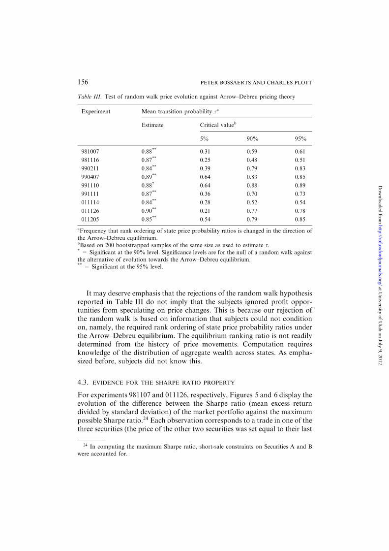
It may deserve emphasis that the rejections of the random walk hypothesisreported in Table III do not imply that the subjects ignored profit oppor-tunities from speculating on price changes. This is because our rejection ofthe random walk is based on information that subjects could not conditionon, namely, the required rank ordering of state price probability ratios underthe Arrow–Debreu equilibrium. The equilibrium ranking ratio is not readilydetermined from the history of price movements. Computation requiresknowledge of the distribution of aggregate wealth across states. As empha-sized before, subjects did not know this.

4.3. EVIDENCE FOR THE SHARPE RATIO PROPERTY

For experiments 981107 and 011126, respectively, Figures 5 and 6 display theevolution of the difference between the Sharpe ratio (mean excess returndivided by standard deviation) of the market portfolio against the maximumpossible Sharpe ratio.24 Each observation corresponds to a trade in one of thethree securities (the price of the other two securities was set equal to their last

Table III. Test of random walk price evolution against Arrow–Debreu pricing theory

Experiment Mean transition probability sa

Estimate Critical valueb

5% 90% 95%

981007 0.88** 0.31 0.59 0.61

981116 0.87** 0.25 0.48 0.51

990211 0.84** 0.39 0.79 0.83

990407 0.89** 0.64 0.83 0.85

991110 0.88* 0.64 0.88 0.89

991111 0.87** 0.36 0.70 0.73

011114 0.84** 0.28 0.52 0.54

011126 0.90** 0.21 0.77 0.78

011205 0.85** 0.54 0.79 0.85

aFrequency that rank ordering of state price probability ratios is changed in the direction of

the Arrow–Debreu equilibrium.bBased on 200 bootstrapped samples of the same size as used to estimate s.* = Significant at the 90% level. Significance levels are for the null of a random walk against

the alternative of evolution towards the Arrow–Debreu equilibrium.** = Significant at the 95% level.

24 In computing the maximum Sharpe ratio, short-sale constraints on Securities A and Bwere accounted for.


at University of U


Dow

nloaded from


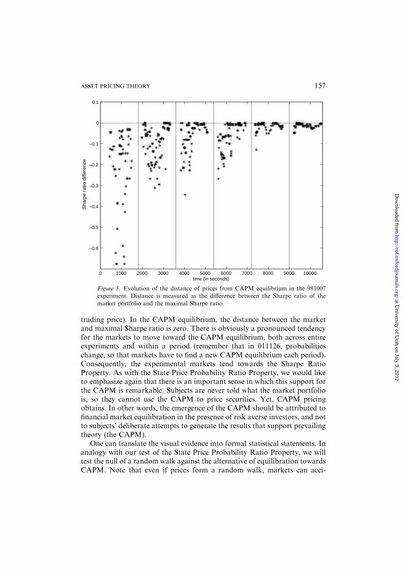
trading price). In the CAPM equilibrium, the distance between the marketand maximal Sharpe ratio is zero. There is obviously a pronounced tendencyfor the markets to move toward the CAPM equilibrium, both across entireexperiments and within a period (remember that in 011126, probabilitieschange, so that markets have to find a new CAPM equilibrium each period).Consequently, the experimental markets tend towards the Sharpe RatioProperty. As with the State Price Probability Ratio Property, we would liketo emphasize again that there is an important sense in which this support forthe CAPM is remarkable. Subjects are never told what the market portfoliois, so they cannot use the CAPM to price securities. Yet, CAPM pricingobtains. In other words, the emergence of the CAPM should be attributed tofinancial market equilibration in the presence of risk averse investors, and notto subjects’ deliberate attempts to generate the results that support prevailingtheory (the CAPM).

One can translate the visual evidence into formal statistical statements. Inanalogy with our test of the State Price Probability Ratio Property, we willtest the null of a random walk against the alternative of equilibration towardsCAPM. Note that even if prices form a random walk, markets can acci-

0 1000 2000 3000 4000 5000 6000 7000 8000 9000 10000

–0.6

–0.5

–0.4

–0.3

–0.2

–0.1

0

0.1

time (in seconds)

Sha

rpe

ratio

diff

eren

ce

Figure 5. Evolution of the distance of prices from CAPM equilibrium in the 981007experiment. Distance is measured as the difference between the Sharpe ratio of themarket portfolio and the maximal Sharpe ratio.


at University of U


Dow

nloaded from


dentally move towards the CAPM equilibrium, i.e., to a point where themarket portfolio is mean–variance optimal. Under the alternative hypothesis,however, this movement is not accidental: the farther away from equilibrium,the more the market is attracted towards equilibrium. We wish to use thisinsight to formally distinguish the two hypotheses, and to test whether thevisual evidence in favor of the CAPM is not a case of mere luck.

Our test works as follows. Let Dt denote the distance between the Sharperatio of the market and the maximum Sharpe ratio at transaction t. Dt is theabsolute value of the variable plotted in Figures 5 and 6. Consider the pro-jection of the change in Dt onto Dt�1:

Dt � Dt�1 ¼ jDt�1 þ �t; ð6Þ

where j is such that �t is uncorrelated with Dt�1. CAPM implies Dt ¼ 0;convergence to CAPM pricing implies j < 0. We then determine the distri-bution of the least squares estimates of j under the null hypothesis of arandom walk, by bootstrapping the empirical joint distribution of changes in

0 1000 2000 3000 4000 5000 6000 7000 8000 9000

–0.6

–0.5

–0.4

–0.3

–0.2

–0.1

0

0.1

time (in seconds)

Sha

rpe

ratio

diff

eren

ce

Figure 6. Evolution of the distance of prices from CAPM equilibrium in the 011126experiment (involving Bulgarian subjects). Distance is measured as the difference be-tween the Sharpe ratio of the market portfolio and the maximal Sharpe ratio.


at University of U


Dow

nloaded from


transaction prices. The null hypothesis of a random walk is rejected (in favorof stochastic convergence to CAPM) if the least squares estimate of j isbeyond a critical value in the left tail of the ensuing distribution. This testingprocedure is a variation of indirect inference (see Gourieroux et al., 1993): wesummarize the data in terms of a simple statistical model (in our case, a leastsquares projection) and determine the distribution of the estimates by sim-ulating the variables entering the statistical model. Instead of simulating off atheoretical distribution, we bootstrap the empirical distribution, however.25

For each experiment, we estimated j using OLS. 5% and 10% criticalvalues under the random walk null hypothesis were determined by boot-strapping form the empirical joint distribution of price changes (we generated200 price series of the same length as the sample used to estimate j).26

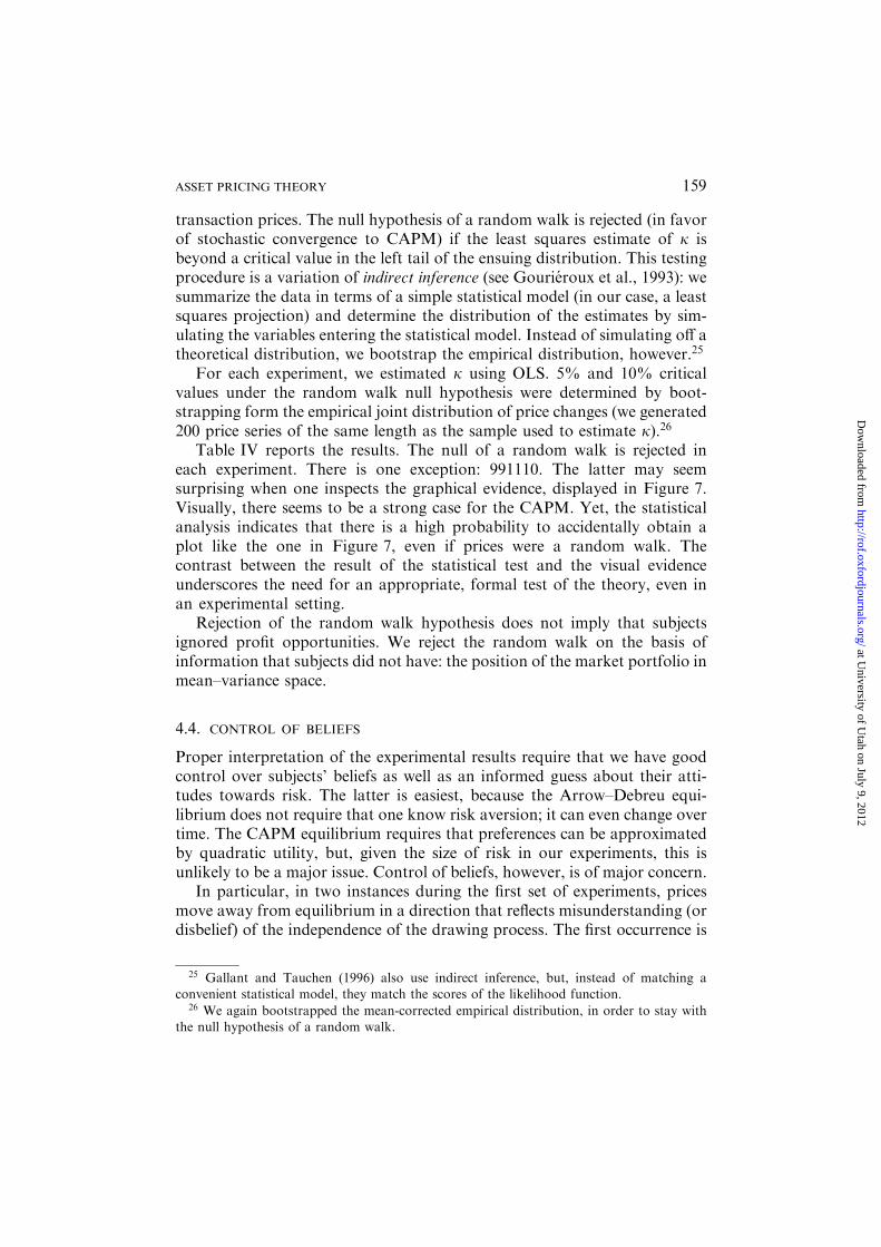
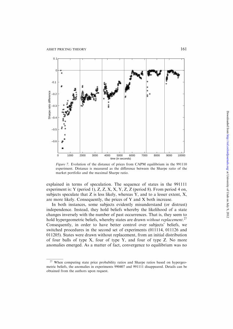
Table IV reports the results. The null of a random walk is rejected ineach experiment. There is one exception: 991110. The latter may seemsurprising when one inspects the graphical evidence, displayed in Figure 7.Visually, there seems to be a strong case for the CAPM. Yet, the statisticalanalysis indicates that there is a high probability to accidentally obtain aplot like the one in Figure 7, even if prices were a random walk. Thecontrast between the result of the statistical test and the visual evidenceunderscores the need for an appropriate, formal test of the theory, even inan experimental setting.

Rejection of the random walk hypothesis does not imply that subjectsignored profit opportunities. We reject the random walk on the basis ofinformation that subjects did not have: the position of the market portfolio inmean–variance space.

4.4. CONTROL OF BELIEFS

Proper interpretation of the experimental results require that we have goodcontrol over subjects’ beliefs as well as an informed guess about their atti-tudes towards risk. The latter is easiest, because the Arrow–Debreu equi-librium does not require that one know risk aversion; it can even change overtime. The CAPM equilibrium requires that preferences can be approximatedby quadratic utility, but, given the size of risk in our experiments, this isunlikely to be a major issue. Control of beliefs, however, is of major concern.

In particular, in two instances during the first set of experiments, pricesmove away from equilibrium in a direction that reflects misunderstanding (ordisbelief) of the independence of the drawing process. The first occurrence is

25 Gallant and Tauchen (1996) also use indirect inference, but, instead of matching aconvenient statistical model, they match the scores of the likelihood function.

26 We again bootstrapped the mean-corrected empirical distribution, in order to stay withthe null hypothesis of a random walk.


at University of U


Dow

nloaded from


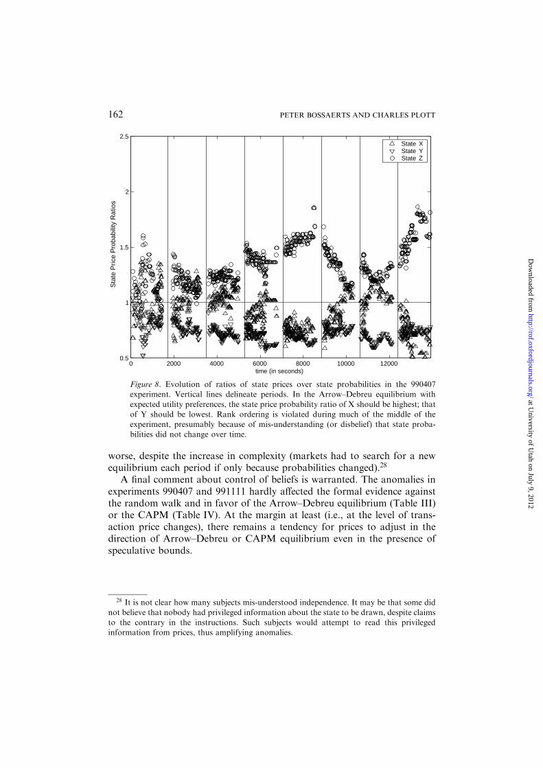
in experiment 990407. The plot of the evolution of state prices (normalized toadd up to 1) will make this clear. Figure 8 shows that the price of state Y isgenerally lowest, but that the ranking of states X and Z is wrong during mostof the middle part of the experiment. An explanation for the reversal of theordering of the prices for states X and Z emerges once it is contrasted withthe sequencing of the states. The sequence of states in 990407 is: X (period 1),Y, Y, X, Z, Y, X, Y (period 8). By the fourth period, some subjects evidentlybecome convinced that period Z is more likely to be drawn next, because ithas not yet appeared (of course, this is incorrect). These subjects implicitlybid up the price of state Z. Their view of the world (that the likelihood of astate depends inversely on the number of times it is drawn in the past) seemsto be confirmed at the end of period 5. As a result, by period 8, speculationabout Z re-emerges. Again, they implicitly bid up the price of state Z, makingit hard for the market to move to an Arrow–Debreu equilibrium.

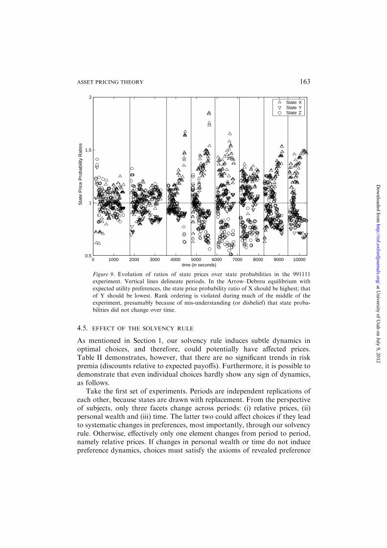
The second instance in which subjective beliefs deviated from objectiveprobabilities is around the middle of experiment 991110. The evolution ofstate prices is plotted in Figure 9. Notice how the price of state X is generallyhighest, as predicted in the Arrow–Debreu equilibrium, but that the rankingof the prices of states Y and Z is wrong in periods 3–6. Again this may be

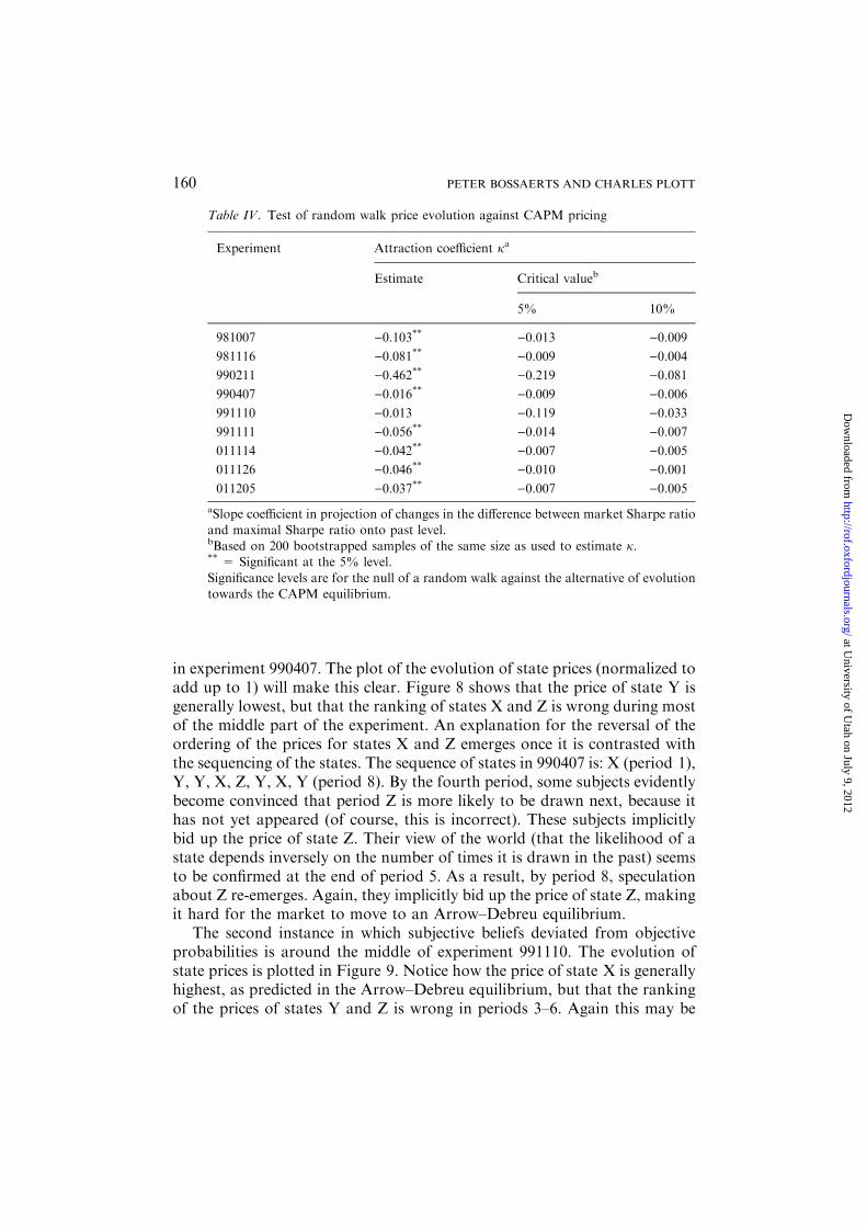
Table IV. Test of random walk price evolution against CAPM pricing

Experiment Attraction coefficient ja

Estimate Critical valueb

5% 10%

981007 )0.103** )0.013 )0.009981116 )0.081** )0.009 )0.004990211 )0.462** )0.219 )0.081990407 )0.016** )0.009 )0.006991110 )0.013 )0.119 )0.033991111 )0.056** )0.014 )0.007011114 )0.042** )0.007 )0.005011126 )0.046** )0.010 )0.001011205 )0.037** )0.007 )0.005

aSlope coefficient in projection of changes in the difference between market Sharpe ratio

and maximal Sharpe ratio onto past level.bBased on 200 bootstrapped samples of the same size as used to estimate j.** = Significant at the 5% level.

Significance levels are for the null of a random walk against the alternative of evolutiontowards the CAPM equilibrium.


at University of U


Dow

nloaded from


explained in terms of speculation. The sequence of states in the 991111experiment is: Y (period 1), Z, Z, X, X, Y, Z, Z (period 8). From period 4 on,subjects speculate that Z is less likely, whereas Y, and to a lesser extent, X,are more likely. Consequently, the prices of Y and X both increase.

In both instances, some subjects evidently misunderstand (or distrust)independence. Instead, they hold beliefs whereby the likelihood of a statechanges inversely with the number of past occurrences. That is, they seem tohold hypergeometric beliefs, whereby states are drawn without replacement.27

Consequently, in order to have better control over subjects’ beliefs, weswitched procedures in the second set of experiments (011114, 011126 and011205). States were drawn without replacement, from an initial distributionof four balls of type X, four of type Y, and four of type Z. No moreanomalies emerged. As a matter of fact, convergence to equilibrium was no

0 1000 2000 3000 4000 5000 6000 7000 8000 9000 10000

–0.6

–0.5

–0.4

–0.3

–0.2

-0.1

0

0.1

time (in seconds)

Sha

rpe

ratio

diff

eren

ce

Figure 7. Evolution of the distance of prices from CAPM equilibrium in the 991110experiment. Distance is measured as the difference between the Sharpe ratio of the

market portfolio and the maximal Sharpe ratio.

27 When computing state price probability ratios and Sharpe ratios based on hypergeo-

metric beliefs, the anomalies in experiments 990407 and 991111 disappeared. Details can beobtained from the authors upon request.


at University of U


Dow

nloaded from


worse, despite the increase in complexity (markets had to search for a newequilibrium each period if only because probabilities changed).28

A final comment about control of beliefs is warranted. The anomalies inexperiments 990407 and 991111 hardly affected the formal evidence againstthe random walk and in favor of the Arrow–Debreu equilibrium (Table III)or the CAPM (Table IV). At the margin at least (i.e., at the level of trans-action price changes), there remains a tendency for prices to adjust in thedirection of Arrow–Debreu or CAPM equilibrium even in the presence ofspeculative bounds.

0 2000 4000 6000 8000 10000 120000.5

1

1.5

2

2.5

time (in seconds)

Sta

te P

rice

Pro

babi

lity

Rat

ios


Figure 8. Evolution of ratios of state prices over state probabilities in the 990407experiment. Vertical lines delineate periods. In the Arrow–Debreu equilibrium withexpected utility preferences, the state price probability ratio of X should be highest; that

of Y should be lowest. Rank ordering is violated during much of the middle of theexperiment, presumably because of mis-understanding (or disbelief) that state proba-bilities did not change over time.

28 It is not clear how many subjects mis-understood independence. It may be that some didnot believe that nobody had privileged information about the state to be drawn, despite claims

to the contrary in the instructions. Such subjects would attempt to read this privilegedinformation from prices, thus amplifying anomalies.


at University of U


Dow

nloaded from


4.5. EFFECT OF THE SOLVENCY RULE

As mentioned in Section 1, our solvency rule induces subtle dynamics inoptimal choices, and therefore, could potentially have affected prices.Table II demonstrates, however, that there are no significant trends in riskpremia (discounts relative to expected payoffs). Furthermore, it is possible todemonstrate that even individual choices hardly show any sign of dynamics,as follows.

Take the first set of experiments. Periods are independent replications ofeach other, because states are drawn with replacement. From the perspectiveof subjects, only three facets change across periods: (i) relative prices, (ii)personal wealth and (iii) time. The latter two could affect choices if they leadto systematic changes in preferences, most importantly, through our solvencyrule. Otherwise, effectively only one element changes from period to period,namely relative prices. If changes in personal wealth or time do not inducepreference dynamics, choices must satisfy the axioms of revealed preference

0 1000 2000 3000 4000 5000 6000 7000 8000 9000 100000.5

1

1.5

2

time (in seconds)

Sta

te P

rice

Pro

babi

lity

Rat

ios


Figure 9. Evolution of ratios of state prices over state probabilities in the 991111experiment. Vertical lines delineate periods. In the Arrow–Debreu equilibrium withexpected utility preferences, the state price probability ratio of X should be highest; that

of Y should be lowest. Rank ordering is violated during much of the middle of theexperiment, presumably because of mis-understanding (or disbelief) that state proba-bilities did not change over time.


at University of U


Dow

nloaded from


(provided that they are optimal, of course). We now show that actual choicesindeed never violate the axioms of revealed preferences for 1/4 of the subjects,and that they violate these axioms insignificantly in most other cases. In otherwords, in the vast majority, subjects’ choices can be almost perfectly ratio-nalized as if coming from a single (quasiconcave) utility function unaffectedby changes in wealth and/or time. This also means that our solvency ruledoes not induce significant dynamics in choices.29

Our results are based on an extension of methodology suggested by An-dreoni and Miller (2002). We use ideas originally introduced by Afriat (1973).Let t ¼ 1; . . . ;T index periods. Let pt denote the vector of prices of securitiesat the end of period t (the price of the riskfree security is set equal to 100). Letxt denote the vector of a subject’s securities holdings at the end of period t(cash holdings are converted to holdings of riskfree securities at the price of100 francs per unit). A subject’s choices can be rationalized as the constrainedmaximization of some quasiconcave utility function if there exist numbersUt � 0 and kt � 1 such that30

Ut �Ut0 � kt0pt0 ðxt � xt0 Þ; ð7Þ

for t; t0 ¼ 1; . . . ;T; t 6¼ t0.We propose to measure failure by means of a slack variable e. If e ¼ 0, the

Afriat inequalities hold. If e > 0, they fail, and e is the minimum income thathas to be taken away from the subject in at least one period (but at mostT� 1 periods) for the Afriat inequalities to hold. e solves the following non-linear programming problem.

min e; ð8Þ

29 It may be surprising that preferences appear to be fixed during the course of an experi-

ment despite our solvency rule. We are not claiming that subjects ignored the solvency rule.Instead, we are showing evidence that the effect of the solvency rule is insignificant. Ananalogy with experiments in physics is appropriate. Newtonian physics makes predictions

about the movement of objects in a vacuum. On earth, it is impossible to create a perfectvacuum, because friction is always present. In the laboratory, however, it is possible to createconditions such that Newtonian physics makes valid predictions despite the presence of

friction. We generated an anologous situation in our financial markets experiments. Staticasset pricing theory explains the experimental results despite the fact that it ignores thepreference dynamics that our solvency rule induces.

30 In Afriat’s original formulation, the restriction on kt is strict positivity (kt > 0). Inspectionof the Afriat inequalities, however, reveals that the scale of the Uts and kts is arbitrary, so thatwe can require kt � 1. At the same time, this ensures that kt is strictly positive. The constraint

on kt is thereby converted to a weak inequality, which facilitates numerical verification of theinequalities.


at University of U


Dow

nloaded from


Ut0 �Ut � kt0 pt0 � xt0 � e� pt0 � xt½ � t; t0 ¼ 1; . . . ;T; t 6¼ t0;

e � 0;

kt0 � 1 t0 ¼ 1; . . . ;T;

Ut � 0 t ¼ 1; . . . ;T:

Table V provides details of the distribution of violations of the Afriatinequalities for the six experiments in the first set. Of the 243 total of activesubjects (two subjects never changed positions and were excluded from theanalysis), one quarter (62) do not violate any of the Afriat inequalities. Themajority ð62þ 79Þ have violations of no more than 25 US cents. This meansthat choices of the majority of subjects can be rationalized in terms of a time-invariant quasiconcave preference profile provided one is willing to shift thevalue of their holdings in at least one period by at most 25 US cents. This isinsignificant relative to the typical total value of their holdings in any period,which is more than US $50. Very few subjects (13) have violations of morethan US $3. The highest violation is US $5.76.31

In evaluating violations of revealed preference, one has to keep in mindthat they have been computed assuming that subjects could trade at lasttransaction prices while subjects’ actual choices may have been based onslightly different prices. In addition, the anomalous belief dynamics reflectedin prices in some of the experiments (see Section 4.4) must have their origin inanomalous choices at the individual level, and hence, could also explain someof the violations. Finally, the above exercise is limited to the first set ofexperiments. In the second set of experiments, not only do relative priceschange, but also probabilities. Choices therefore change not only becauseprices change, but also because beliefs change. Hence, axioms of revealedpreference can no longer be checked.

31 To get a further feeling for the meaning of violations of the Afriat inequalities, takeexperiment 990407, for instance. Consider a subject who is endowed with the market portfolio(expressed per capita) and 400 francs cash. Take the relative prices at the end of periods 1 and

5 (see Table 2). Imagine that this subject invests all wealth in security A when it was mostexpensive (period 1), while rebalancing all wealth into security B when it became mostexpensive (at the end of period 5). To do this, this subject sells all other securities, and borrowsmoney (sells short Notes) up to the short-sale constraint (8 Notes). Such an investment policy

may be chosen if the subject erroneously thinks that the higher the price of an asset, the morelikely it will pay its highest possible dividend. Clearly, this subject violates the Afriatinequalities. The slack variable that solves the non-linear programming problem in Equa-

tion (8) equals 282 francs, or about US $10. No subject in our experiments generated a slackvariable as high this.


at University of U


Dow

nloaded from


4.6. EFFECT OF MARKET THICKNESS

Relative to standards in experimental economics, the experiments we havebeen discussing here are large-scale. Previously, our own (CAPM) exper-iments involved only 5–13 subjects; see Bossaerts and Plott (2002). Whilethese numbers are generally considered to be sufficient to generate Walr-asian equilibrium outcomes, such consensus is based on much simplersettings: one good/security and no uncertainty. In contrast, here we havethree securities, and we let subjects’ natural attitudes towards uncertaintydetermine pricing. This appears to have a marked effect on pricing. Theresults of the thin-markets experiments in Bossaerts and Plott (2002) aresubstantially less compelling as far as general equilibrium theory is con-cerned.

To illustrate how different the results are, Table VI displays medians32

of the distance from CAPM pricing for: (i) the seven thin-market exper-iments in Bossaerts and Plott (2002) (where there were 5–13 subjects), (ii)six thick-market experiments reported on here (where there were between19 and 63 subjects).33 The distance from CAPM pricing is measured as thedifference between the maximum Sharpe ratio and the Sharpe ratio of themarket portfolio. Standard deviations (of the medians) across experimentsare in parentheses. With the exception of the first two periods, the thick-market experiments produce pricing that is significantly closer to CAPMpricing.

5. Conclusion

The experiments demonstrate that the basic principles of modern assetpricing theory are very much at work in competitive financial markets. Pricestend towards a pattern where risk premia are determined solely by covariance

Table V. Frequency of violations of afriat inequalities – experiments with state drawing oftype I

Size of Violations (e), in U.S. dollara

e = 0 0 < e � US $0.25 US $0:25 < e � US $1 US $1 < e � $ 2 $ 2 < e� $ 3 $ 3 < e

62b 79 44 31 14 13

ae in the non-linear programming problem in (8).bNumber of subjects in the category e=0.

32 If the median fell between two outcomes, the lower of the two outcomes is reported.33 Results for the six experiments in the first set are shown here, because only those are

directly comparable to the ones in Bossaerts and Plott (2002), where states were always drawnwith replacement.


at University of U


Dow

nloaded from


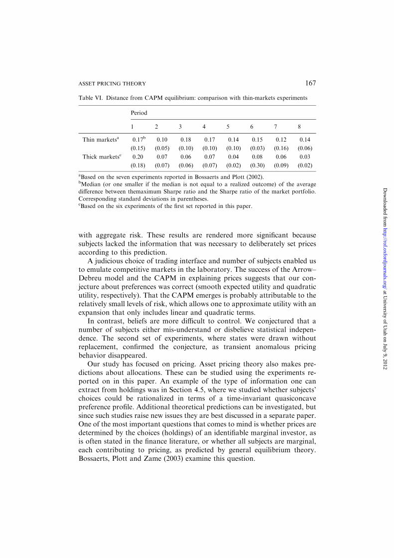
with aggregate risk. These results are rendered more significant becausesubjects lacked the information that was necessary to deliberately set pricesaccording to this prediction.

A judicious choice of trading interface and number of subjects enabled usto emulate competitive markets in the laboratory. The success of the Arrow–Debreu model and the CAPM in explaining prices suggests that our con-jecture about preferences was correct (smooth expected utility and quadraticutility, respectively). That the CAPM emerges is probably attributable to therelatively small levels of risk, which allows one to approximate utility with anexpansion that only includes linear and quadratic terms.

In contrast, beliefs are more difficult to control. We conjectured that anumber of subjects either mis-understand or disbelieve statistical indepen-dence. The second set of experiments, where states were drawn withoutreplacement, confirmed the conjecture, as transient anomalous pricingbehavior disappeared.

Our study has focused on pricing. Asset pricing theory also makes pre-dictions about allocations. These can be studied using the experiments re-ported on in this paper. An example of the type of information one canextract from holdings was in Section 4.5, where we studied whether subjects’choices could be rationalized in terms of a time-invariant quasiconcavepreference profile. Additional theoretical predictions can be investigated, butsince such studies raise new issues they are best discussed in a separate paper.One of the most important questions that comes to mind is whether prices aredetermined by the choices (holdings) of an identifiable marginal investor, asis often stated in the finance literature, or whether all subjects are marginal,each contributing to pricing, as predicted by general equilibrium theory.Bossaerts, Plott and Zame (2003) examine this question.

Table VI. Distance from CAPM equilibrium: comparison with thin-markets experiments

Period

1 2 3 4 5 6 7 8

Thin marketsa 0.17b 0.10 0.18 0.17 0.14 0.15 0.12 0.14

(0.15) (0.05) (0.10) (0.10) (0.10) (0.03) (0.16) (0.06)

Thick marketsc 0.20 0.07 0.06 0.07 0.04 0.08 0.06 0.03

(0.18) (0.07) (0.06) (0.07) (0.02) (0.30) (0.09) (0.02)

aBased on the seven experiments reported in Bossaerts and Plott (2002).bMedian (or one smaller if the median is not equal to a realized outcome) of the averagedifference between themaximum Sharpe ratio and the Sharpe ratio of the market portfolio.

Corresponding standard deviations in parentheses.cBased on the six experiments of the first set reported in this paper.


at University of U


Dow

nloaded from


Finally, there is an urgent need to understand how prices manage to moveto equilibrium. The present paper demonstrates that prices move in the rightdirection, leaving open the question of why. In particular, what role doagents’ choices play? A first exploration can be found in Asparouhova,Bossaerts and Plott (2003). An explicit model and its implications forempirical analysis of asset pricing theory on field data can be found inBossaerts (2003). Elements of the theory proposed in Crockett, Spear andSunder (2002) may provide insights of how repetition of identically the sameenvironment (as in our first set of experiments) eventually leads to equilib-rium pricing.

References

Afriat, S. N. (1973) On a system of inequalities in demand analysis: An extension of theclassical method, International Economic Review 14, 460–472.

Andreoni, J. and Miller J. (2002) Giving according to GARP: An experimental test of theconsistency of preferences for Altruism, Econometrica 70, 737–753.

Asparouhova, E., Bossaerts, P., and Plott, C. (2003) Excess demand and equilibration in

multi-security financial markets: The empirical evidence, Journal of Financial Markets 6,1–22.

Bachelier, L. (1900) Theorie de la Speculation, Annales Scientifiques de l’ Ecole Normale

Superieure III-17, 21–86.Barberis, N., Huang, M., and Santos, T. (2001) Prospect theory and asset prices, Quarterly

Journal of Economics 116, 1–53.Biais, B., Bossaerts, P., and Spatt, C. (2003) Equilibrium asset pricing under heterogeneous

information, CMU Working Paper.Bossaerts, P. (2003) Testing CAPM in real markets: Implications from experiments, Caltech

Working Paper.

Bossaerts, P., Fine, L., and Ledyard, J. (2002) Inducing liquidity in thin financial marketsthrough combined-value trading mechanisms, European Economic Review 46, 1671–1695.

Bossaerts, P., Kleiman, D., and Plott, C. (2002) Price discovery in financial markets: The caseof the CAPM, in (ed.), C. Plott Collected papers on the Foundations of ExperimentalEconomics and Political Science: Information, Finance and General Equilibrium, Volume.

III, Edwin Elgar Publishers.Bossaerts, P., Plott, C., and Zame, W. (2003), Prices and portfolio choices in financial markets:

theory and experiments, Caltech/UCLA Working Paper.Bossaerts, P. and Plott, C. (2002) The CAPM in thin experimental financial markets, Journal

of Economics Dynamics and Control 26, 1093–1112.Clower, R. (1967) A re-consideration of the microfoundations of monetary theory, Western

Economic Journal 6, 1–9.

Crockett, S. Spear, S., and Sunder, S. (2002) A simple decentralized institution for learningcompetitive equilibrium, Yale ICF Working Paper.

Debreu, G. (1959): Theory of Value, New York, Wiley.

Dybvig, P. and Ingersoll, J. (1982) Mean–variance theory in complete markets, Journal ofBusiness 55, 233–251.


at University of U


Dow

nloaded from


Epstein, L. and Zin, S. (2001) The independence axiom and asset returns, Journal of EmpiricalFinance 8, 537–572.

Gallant, R.A. and Tauchen, G. (1996) Which moments to match? Econometric Theory 12,657–681.

Gourieroux, C., Monfort, A., and Renault, E. (1993) Indirect inference, Journal of Applied

Econometrics 8, S85–S118.Holt, C. and Laury, S. (2002) Risk aversion and incentive effects, American Economic Review

92, 1644–1655.Kroll, Y., Levy, H., and Rapaport, A. (1988) Experimental tests of the separation theorem

and the capital asset pricing model,’’ American Economic Review 78, 500–519.Levy, H. (1997) Risk and return: An experimental analysis, International Economic Review 38,

119–149.

Lintner, J. (1965) The valuation of risk assets and the selection of risky investments in stockportfolios and capital budgets, Review of Economics and Statistics 47, 13–37.

Lucas, R. (1982) Interest rates and currency prices in a two-country world, Journal of

Monetary Economics 10, 335–59.Mossin, J. (1966) Equilibrium in a capital asset market Econometrica 34, 768–83.Noussair, C., Plott, C. and Riezman, R. (1997) The principles of exchange rate determination

in an international Finance experiment, Journal of Political Economy 105, 822–861.

Roll, R. (1977) A critique of the asset pricing theory’s tests, Part I: On the past and potentialtestability of the theory, Journal of Financial Economics 4, 129–76.

Sharpe, W. (1964) Capital asset prices: A theory of market equilibrium under conditions of

risk, Journal of Finance 19, 425–442.


at University of U


Dow

nloaded from


Basic Principles of Asset Pricing Theory: Evidence from...

Documents

Transcript of Basic Principles of Asset Pricing Theory: Evidence from...