Basic Models of Probability
24
03/16/22 (c) 2000, Ron S. Kenett, Ph.D. 1 asic Models of Probabilit Instructor: Ron S. Kenett Email: [email protected] Course Website: www.kpa.co.il/biostat Course textbook: MODERN INDUSTRIAL STATISTICS, Kenett and Zacks, Duxbury Press, 1998
-
Upload
cynthia-soto -
Category
Documents
-
view
31 -
download
2
description
Basic Models of Probability. Instructor: Ron S. Kenett Email: [email protected] Course Website: www.kpa.co.il/biostat Course textbook: MODERN INDUSTRIAL STATISTICS, Kenett and Zacks, Duxbury Press, 1998. Course Syllabus. Understanding Variability Variability in Several Dimensions - PowerPoint PPT Presentation
Transcript of Basic Models of Probability

04/20/23
(c) 2000, Ron S. Kenett, Ph.D. 1
Basic Models of Probability
Instructor: Ron S. KenettEmail: [email protected]
Course Website: www.kpa.co.il/biostatCourse textbook: MODERN INDUSTRIAL STATISTICS,
Kenett and Zacks, Duxbury Press, 1998

04/20/23
(c) 2000, Ron S. Kenett, Ph.D. 2
Course Syllabus
•Understanding Variability•Variability in Several Dimensions•Basic Models of Probability•Sampling for Estimation of Population Quantities•Parametric Statistical Inference•Computer Intensive Techniques•Multiple Linear Regression•Statistical Process Control•Design of Experiments

04/20/23
(c) 2000, Ron S. Kenett, Ph.D. 3
The Paradox of the Chevalier de Mere - 1
Success = at least one “1”

04/20/23
(c) 2000, Ron S. Kenett, Ph.D. 4
Success = at least one “1,1”
The Paradox of the Chevalier de Mere - 2

04/20/23
(c) 2000, Ron S. Kenett, Ph.D. 5
P (Success) = P(at least one “1,1”)
The Paradox of the Chevalier de Mere - 3
P (Success) = P(at least one “1”)
32
614 3
236
124
Experience proved otherwise !Experience proved otherwise !Experience proved otherwise !Experience proved otherwise !
Game A was a better game to play

04/20/23
(c) 2000, Ron S. Kenett, Ph.D. 6
The Paradox of the Chevalier de Mere - 4
P (Failure) = P(no “1”)
482.65 4
What went wrong before?What went wrong before?What went wrong before?What went wrong before?
P (Success) = .518P (Success) = .518
P (Failure) = P(no “1,1”)
509.3635 24
P (Success) = .491P (Success) = .491
The calculations of Pascal and Fermat

04/20/23
(c) 2000, Ron S. Kenett, Ph.D. 7
To add or to multiply ?
P(outcomes add up to “10”) P(outcomes add up to “10”) ==??

04/20/23
(c) 2000, Ron S. Kenett, Ph.D. 8
P(outcomes add up to “10”) P(outcomes add up to “10”) 36 / 3 =36 / 3 =
1,1 1,2 1,3 1,4 1,5 1,62,1 2,2 2,3 2,4 2,5 2,63,1 3,2 3,2 3,4 3,5 3,64,1 4,2 4,3 4,4 4,5 4,65,1 5,2 5,3 5,4 5,5 5,66,1 6,2 6,3 6,4 6,5 6,6
04/20/23
(c) 2000, Ron S. Kenett, Ph.D. 9
Mutually Exclusive EventsMutually Exclusive Events
Two events are mutually exclusive (or disjoint) if it is impossible for them to occur together.
If two events are mutually exclusive, they cannot be independent and vice versa.
Example:A subject in a study cannot be both male and female, nor can they be aged 20 and 30. A subject could however be both male and 20, both female and 30.

04/20/23
(c) 2000, Ron S. Kenett, Ph.D. 10
Independent EventsIndependent Events
Two events are independent if the occurrence of one of the events gives us no information about whether or not the other event will occur; that is, the events have no influence on each other.
If two events are independent then they cannot be mutually exclusive (disjoint) and vice versa.
04/20/23
(c) 2000, Ron S. Kenett, Ph.D. 11
ExampleSuppose that a man and a woman each have a pack of 52 playing cards. Each draws a card from his/her pack. Find the probability that they each draw the ace of clubs.
We define the events
A = 'the man draws the ace of clubs'B = 'the woman draws the ace of clubs'
Clearly events A and B are independent so,That is, there is a very small chance that the man and the woman will both draw the ace of clubs.

04/20/23
(c) 2000, Ron S. Kenett, Ph.D. 12
Conditional ProbabilityConditional Probability
In many situations, once more information becomes available, we are able to revise our estimates for the probability of further outcomes or events happening. For example, suppose you go out for lunch at the same place and time every Friday and you are served lunch within 15 minutes with probability 0.9. However, given that you notice that the restaurant is exceptionally busy, the probability of being served lunch within 15 minutes may reduce to 0.7. This is the conditional probability of being served lunch within 15 minutes given that the restaurant is exceptionally busy.

04/20/23
(c) 2000, Ron S. Kenett, Ph.D. 13
The usual notation for "event A occurs given that event B has occurred" is A|B (A given B). The symbol | is a vertical line and does not imply division. P(A|B) denotes the probability that event A will occur given that event B has occurred already.
A rule that can be used to determine a conditional probability from unconditional probabilities is
P(A|B) = P(A and B) / P(B)
where,P(A|B) = the (conditional) probability that event A will occur given that event B has occurred alreadyP(A and B) = the (unconditional) probability that event A and event B occurP(B) = the (unconditional) probability that event B occurs

04/20/23
(c) 2000, Ron S. Kenett, Ph.D. 14
X = Number of successes in n trials
xnpxpxnx
nxP
)1()!(!
! )(
n = 6, x = 0
n = 6, x = 1
n = 6, x = 3 x0 n
Binomial DistributionBinomial Distribution

04/20/23
(c) 2000, Ron S. Kenett, Ph.D. 15
Binomial DistributionBinomial Distribution
0 10 20 30 40 50
0.00
0.05
0.10
i
b(i;
50
, p)
p=.25
p=.5
p=.75
0 10 20 30 40 50
0.00
0.05
0.10
i
b(i;
50
, p)
p=.25
p=.5
p=.75

04/20/23
(c) 2000, Ron S. Kenett, Ph.D. 16
Binomial DistributionBinomial Distribution
7 9 11 13 15 17 19 21
0
10
20
30
C1
Pe
rce
nt
0 10 20 30 40 50
0.00
0.05
0.10
i
b(i;
50
, p)
p=.25
p=.5
p=.75
0 10 20 30 40 50
0.00
0.05
0.10
i
b(i;
50
, p)
p=.25
p=.5
p=.75
13 16 20 11 1210 12 20 16 1510 12 9 18 1211 11 9 11 1413 8 4 13 1214 11 14 15 12
18 13 7 11 915 11 8 11 169 12 12 18 1513 9 15 12 12
13 16 20 11 1210 12 20 16 1510 12 9 18 1211 11 9 11 1413 8 4 13 1214 11 14 15 12
18 13 7 11 915 11 8 11 169 12 12 18 1513 9 15 12 12
04/20/23
(c) 2000, Ron S. Kenett, Ph.D. 17
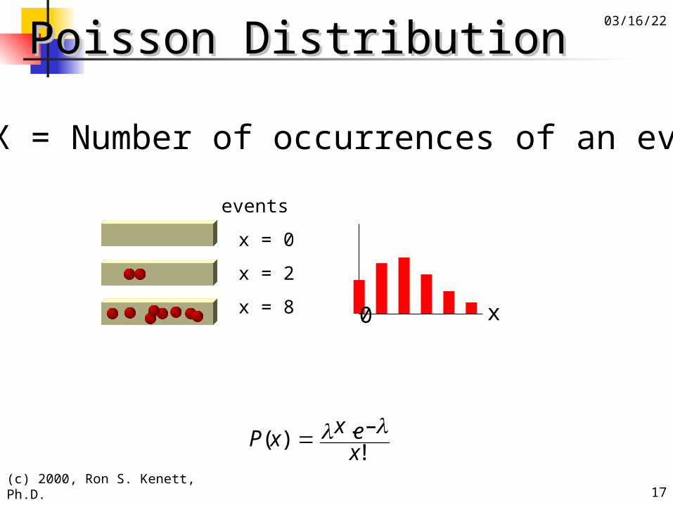
Poisson DistributionPoisson Distribution
P(x) xe–x!
x = 0
x = 2
x = 8 x0
events
X = Number of occurrences of an event

04/20/23
(c) 2000, Ron S. Kenett, Ph.D. 18
Poisson DistributionPoisson Distribution
50403020100
0.2
0.1
0.0
j
p(j;
lam
bda
)
lambda=5
lambda=10
lambda=15
50403020100
0.2
0.1
0.0
j
p(j;
lam
bda
)
lambda=5
lambda=10
lambda=15
04/20/23
(c) 2000, Ron S. Kenett, Ph.D. 19
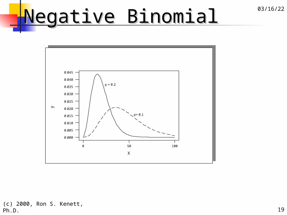
Negative BinomialNegative Binomial
0 50 100
0.000
0.005
0.010
0.015
0.020
0.025
0.030
0.035
0.040
0.045
X
y
p = 0.2
p= 0.1
0 50 100
0.000
0.005
0.010
0.015
0.020
0.025
0.030
0.035
0.040
0.045
X
y
p = 0.2
p= 0.1

04/20/23
(c) 2000, Ron S. Kenett, Ph.D. 20
Normal DistributionNormal Distribution
0 10 20
0.0
0.1
0.2
0.3
0.4
x
y
Sigma = 1
Sigma = 2
Sigma = 3
0 10 20
0.0
0.1
0.2
0.3
0.4
x
y
Sigma = 1
Sigma = 2
Sigma = 3
04/20/23
(c) 2000, Ron S. Kenett, Ph.D. 21
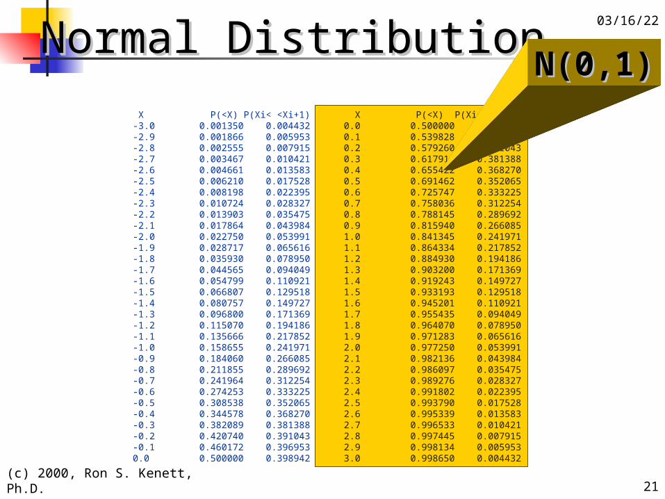
Normal DistributionNormal Distribution
X P(<X) P(Xi< <Xi+1)-3.0 0.001350 0.004432-2.9 0.001866 0.005953-2.8 0.002555 0.007915-2.7 0.003467 0.010421-2.6 0.004661 0.013583-2.5 0.006210 0.017528-2.4 0.008198 0.022395-2.3 0.010724 0.028327-2.2 0.013903 0.035475-2.1 0.017864 0.043984-2.0 0.022750 0.053991-1.9 0.028717 0.065616-1.8 0.035930 0.078950-1.7 0.044565 0.094049-1.6 0.054799 0.110921-1.5 0.066807 0.129518-1.4 0.080757 0.149727-1.3 0.096800 0.171369-1.2 0.115070 0.194186-1.1 0.135666 0.217852-1.0 0.158655 0.241971-0.9 0.184060 0.266085-0.8 0.211855 0.289692-0.7 0.241964 0.312254-0.6 0.274253 0.333225-0.5 0.308538 0.352065-0.4 0.344578 0.368270-0.3 0.382089 0.381388-0.2 0.420740 0.391043-0.1 0.460172 0.3969530.0 0.500000 0.398942
X P(<X) P(Xi< <Xi+1)0.0 0.500000 0.3989420.1 0.539828 0.3969530.2 0.579260 0.3910430.3 0.617911 0.3813880.4 0.655422 0.3682700.5 0.691462 0.3520650.6 0.725747 0.3332250.7 0.758036 0.3122540.8 0.788145 0.2896920.9 0.815940 0.2660851.0 0.841345 0.2419711.1 0.864334 0.2178521.2 0.884930 0.1941861.3 0.903200 0.1713691.4 0.919243 0.1497271.5 0.933193 0.1295181.6 0.945201 0.1109211.7 0.955435 0.0940491.8 0.964070 0.0789501.9 0.971283 0.0656162.0 0.977250 0.0539912.1 0.982136 0.0439842.2 0.986097 0.0354752.3 0.989276 0.0283272.4 0.991802 0.0223952.5 0.993790 0.0175282.6 0.995339 0.0135832.7 0.996533 0.0104212.8 0.997445 0.0079152.9 0.998134 0.0059533.0 0.998650 0.004432
N(0,1)N(0,1)

04/20/23
(c) 2000, Ron S. Kenett, Ph.D. 22
Normal DistributionNormal Distribution
7.5 8.0 8.5 9.0 9.5 10.0 10.5 11.0 11.5 12.0 12.5
0
10
20
C1
Pe
rce
nt
0 10 20
0.0
0.1
0.2
0.3
0.4
x
y
Sigma = 1
Sigma = 2
Sigma = 3
0 10 20
0.0
0.1
0.2
0.3
0.4
x
y
Sigma = 1
Sigma = 2
Sigma = 3
7.9006 11.5151 9.9542 9.4493 8.238710.4707 9.4041 9.3517 10.5664 10.907910.0077 12.5188 9.6937 10.0757 10.161610.2881 9.8560 10.0014 9.8467 11.5006
10.2982 9.6023 9.7238 11.5413 8.45959.2372 11.0408 12.8996 9.5590 9.1041
8.9170 9.7734 7.9844 8.3484 11.370310.6260 10.0952 11.4019 8.9842 9.37839.7574 7.9312 8.1566 9.9305 9.11588.6436 10.4689 9.3356 10.8788 7.8790

04/20/23
(c) 2000, Ron S. Kenett, Ph.D. 23
The t DistributionThe t Distribution
-5 0 5
0.0
0.1
0.2
0.3
0.4
0.5
t
t(x;
nu)
nu=5
nu=50
-5 0 5
0.0
0.1
0.2
0.3
0.4
0.5
t
t(x;
nu)
nu=5
nu=50

04/20/23
(c) 2000, Ron S. Kenett, Ph.D. 24
The F DistributionThe F Distribution
0 1 2 3 4 5 6
0.0
0.1
0.2
0.3
0.4
0.5
0.6
0.7
x
y
0 1 2 3 4 5 6
0.0
0.1
0.2
0.3
0.4
0.5
0.6
0.7
x
y