BASIC MICROSOFT EXCEL

IT Training Team Jefferson Parish Library

PHONE: 504-838-1144

EMAIL: jpltrain@jplibrary.net

In this class you will learn to:

• Launch and interact with Microsoft Excel 2010

• Create new workbooks

• Navigate through a spreadsheet

• Select cells

• Enter and delete data

• Drag and drop cells

• Work with columns and rows

• Save a workspace

2

Meeting Microsoft Office Excel 2010

What is Microsoft Office Excel 2010?

• Microsoft Office Excel 2010 is the fourteenth

version of Microsoft’s spreadsheet program. A

spreadsheet is essentially a large flexible grid that is

used to hold information, usually numerical.

• Using Excel, you can analyze large amounts of data,

move sets of data around to get a different picture

of your figures, and generate a number of different

charts and diagrams to help summarize the data.

3

LAUNCHING EXCEL

To open Microsoft Office Excel 2010:

• Click the Start menu

• Place your mouse over All Programs.

• Scroll down to the Microsoft Office folder inside the Start menu.

• Hover over it (or click) with your mouse to show a sub-menu, and then click Microsoft Excel 2010.

You can also open Excel if you have an Excel icon on your desktop:

• Double-click the icon to open Excel

4

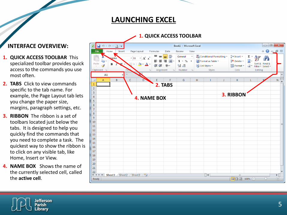
1. QUICK ACCESS TOOLBAR This specialized toolbar provides quick access to the commands you use most often.

2. TABS Click to view commands specific to the tab name. For example, the Page Layout tab lets you change the paper size, margins, paragraph settings, etc.

3. RIBBON The ribbon is a set of toolbars located just below the tabs. It is designed to help you quickly find the commands that you need to complete a task. The quickest way to show the ribbon is to click on any visible tab, like Home, Insert or View.

4. NAME BOX Shows the name of the currently selected cell, called the active cell.

1. QUICK ACCESS TOOLBAR

2. TABS

3. RIBBON 4. NAME BOX

LAUNCHING EXCEL

INTERFACE OVERVIEW:

5

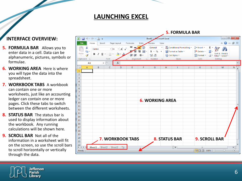
5. FORMULA BAR Allows you to enter data in a cell. Data can be alphanumeric, pictures, symbols or formulae.

6. WORKING AREA Here is where you will type the data into the spreadsheet.

7. WORKBOOK TABS A workbook can contain one or more worksheets, just like an accounting ledger can contain one or more pages. Click these tabs to switch between the different worksheets.

8. STATUS BAR The status bar is used to display information about the workbook. Any running calculations will be shown here.

9. SCROLL BAR Not all of the information in a worksheet will fit on the screen, so use the scroll bars to scroll horizontally or vertically through the data.

7. WORKBOOK TABS

6. WORKING AREA

5. FORMULA BAR

8. STATUS BAR 9. SCROLL BAR

LAUNCHING EXCEL

INTERFACE OVERVIEW:

6

• A column is a vertical series of adjacent cells from top to bottom.

• A row is a horizontal series of cells from left to right.

• A cell describes the intersection of a row and column.

• A cell range is a group of adjacent cells.

COMPONENTS OF A WORKSHEET

The spreadsheet is made up of rows and columns. The intersection of a row and column is called a cell.

7

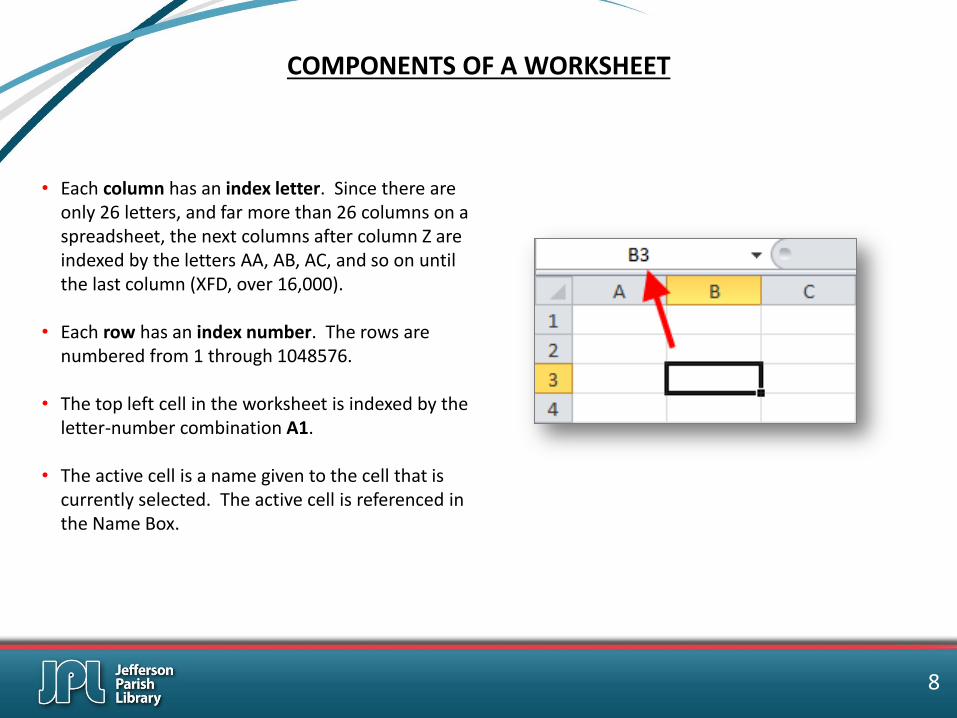
• Each column has an index letter. Since there are only 26 letters, and far more than 26 columns on a spreadsheet, the next columns after column Z are indexed by the letters AA, AB, AC, and so on until the last column (XFD, over 16,000).

• Each row has an index number. The rows are numbered from 1 through 1048576.

• The top left cell in the worksheet is indexed by the letter-number combination A1.

• The active cell is a name given to the cell that is currently selected. The active cell is referenced in the Name Box.

COMPONENTS OF A WORKSHEET

8

• When you click a cell in a worksheet, the border around it becomes thicker.

• The row and column headers are shaded orange, and the cell reference is shown in the Name Box.

• In this image, cell D5 (the one with the thick border) is the active cell.

COMPONENTS OF A WORKSHEET

9

• To select a single cell, just click it.

• To select a group of cells, place your mouse pointer over a cell and then click and hold the left mouse button. Drag the mouse in any direction to select rows, columns, or a combination of each.

• To select an entire row/column of cells, move your mouse over a row/column header. The mouse pointer will turn into an arrow. Then click the header to select that row/column.

WORKING WITH CELLS

10

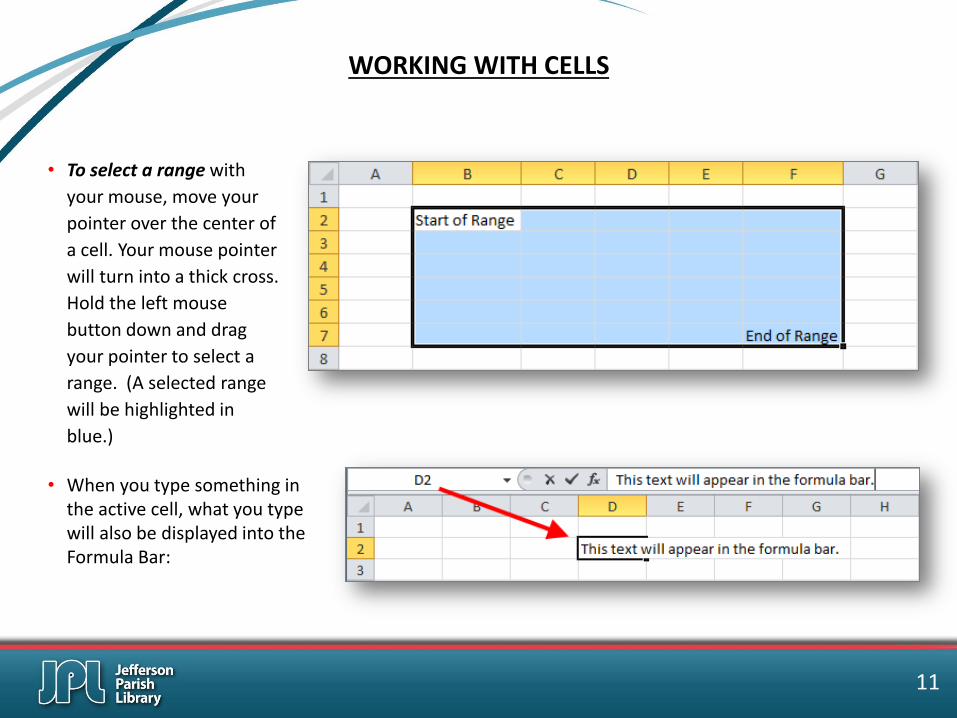
• To select a range with

your mouse, move your

pointer over the center of

a cell. Your mouse pointer

will turn into a thick cross.

Hold the left mouse

button down and drag

your pointer to select a

range. (A selected range

will be highlighted in

blue.)

WORKING WITH CELLS

• When you type something in the active cell, what you type will also be displayed into the Formula Bar:

11

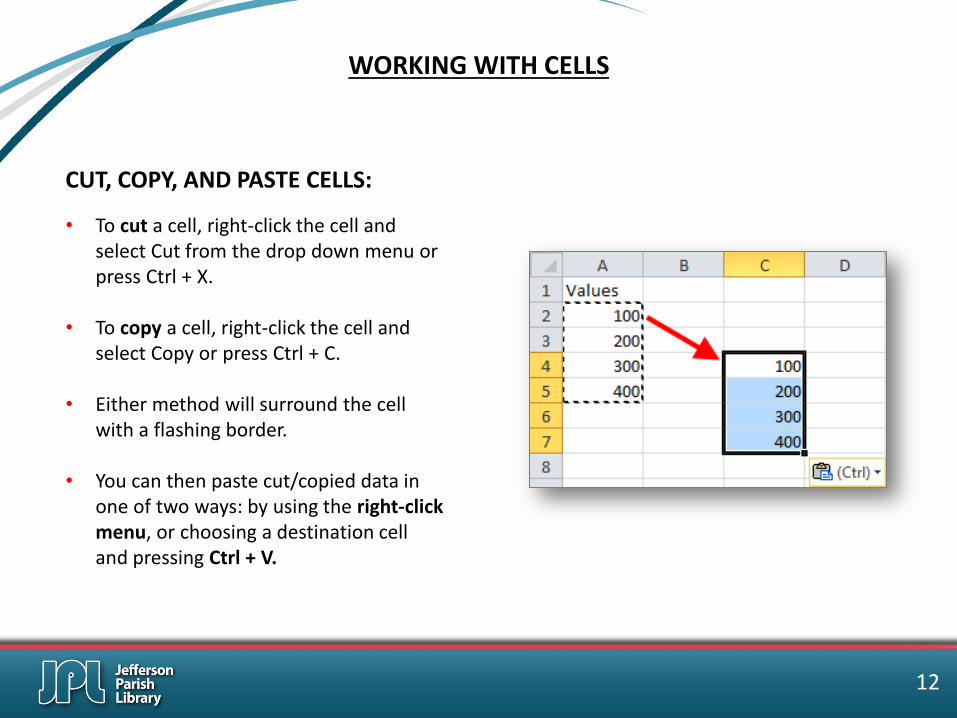
CUT, COPY, AND PASTE CELLS:

• To cut a cell, right-click the cell and select Cut from the drop down menu or press Ctrl + X.

• To copy a cell, right-click the cell and select Copy or press Ctrl + C.

• Either method will surround the cell with a flashing border.

• You can then paste cut/copied data in one of two ways: by using the right-click menu, or choosing a destination cell and pressing Ctrl + V.

WORKING WITH CELLS

12

YOU CAN MOVE A CELL BY DRAGGING AND DROPPING WITH YOUR MOUSE.

• First, select a cell by clicking on it, thereby making it the active cell.

• Now move your mouse pointer over one edge of the active cell border. The mouse pointer will turn into a four-headed arrow.

• Click and drag the cell contents to a new location. Release the mouse button to drop the cell in its new location

WORKING WITH CELLS

13

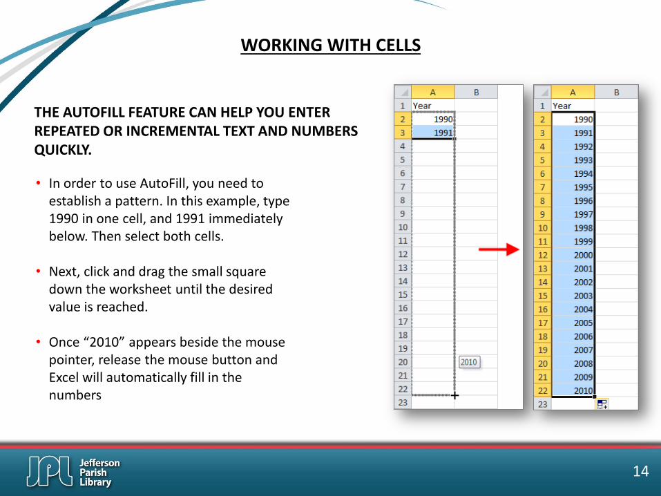
THE AUTOFILL FEATURE CAN HELP YOU ENTER REPEATED OR INCREMENTAL TEXT AND NUMBERS QUICKLY.

• In order to use AutoFill, you need to establish a pattern. In this example, type 1990 in one cell, and 1991 immediately below. Then select both cells.

• Next, click and drag the small square down the worksheet until the desired value is reached.

• Once “2010” appears beside the mouse pointer, release the mouse button and Excel will automatically fill in the numbers

WORKING WITH CELLS

14

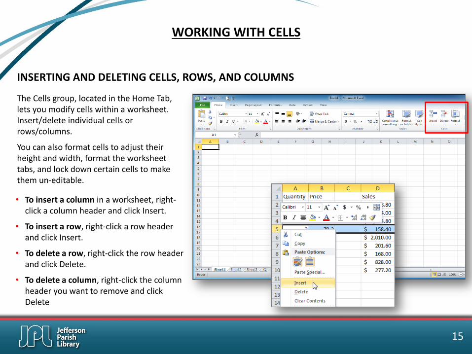
INSERTING AND DELETING CELLS, ROWS, AND COLUMNS

• To insert a column in a worksheet, right-click a column header and click Insert.

• To insert a row, right-click a row header and click Insert.

• To delete a row, right-click the row header and click Delete.

• To delete a column, right-click the column header you want to remove and click Delete

WORKING WITH CELLS

The Cells group, located in the Home Tab, lets you modify cells within a worksheet. Insert/delete individual cells or rows/columns.

You can also format cells to adjust their height and width, format the worksheet tabs, and lock down certain cells to make them un-editable.

15

USE SEPARATORS TO CHANGE THE SIZE OF ROWS OR COLUMNS.

• To change the size of a row or column, place your mouse pointer on the line that divides the column headers. For example, if you wanted to change the size of column B, you would place your mouse pointer on the line separating B and C.

• Your mouse pointer will turn into a line with a small arrow on either side.

• When you see this pointer, click and hold the left mouse button to drag the column edge to the left or right. As you drag you will see the size in pixels.

WORKING WITH CELLS

16

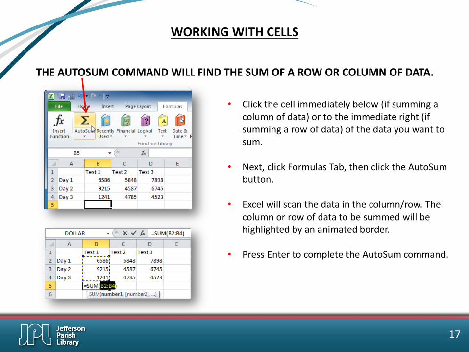
THE AUTOSUM COMMAND WILL FIND THE SUM OF A ROW OR COLUMN OF DATA.

• Click the cell immediately below (if summing a column of data) or to the immediate right (if summing a row of data) of the data you want to sum.

• Next, click Formulas Tab, then click the AutoSum button.

• Excel will scan the data in the column/row. The column or row of data to be summed will be highlighted by an animated border.

• Press Enter to complete the AutoSum command.

WORKING WITH CELLS

17

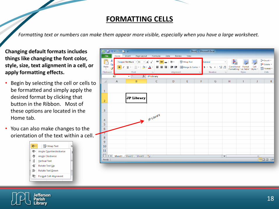
Changing default formats includes things like changing the font color, style, size, text alignment in a cell, or apply formatting effects.

• Begin by selecting the cell or cells to be formatted and simply apply the desired format by clicking that button in the Ribbon. Most of these options are located in the Home tab.

• You can also make changes to the orientation of the text within a cell.

FORMATTING CELLS

Formatting text or numbers can make them appear more visible, especially when you have a large worksheet.

18

The Merge & Center button is a great tool for centering a title over a table of data.

• The Merge & Center button is in

the Alignment group on the Home tab.

• Select the cells you want to merge and center. Then click the Merge & Center button.

• The selected cells will merge into one big cell, and the text will align to the center of the merged cell.

FORMATTING CELLS

19

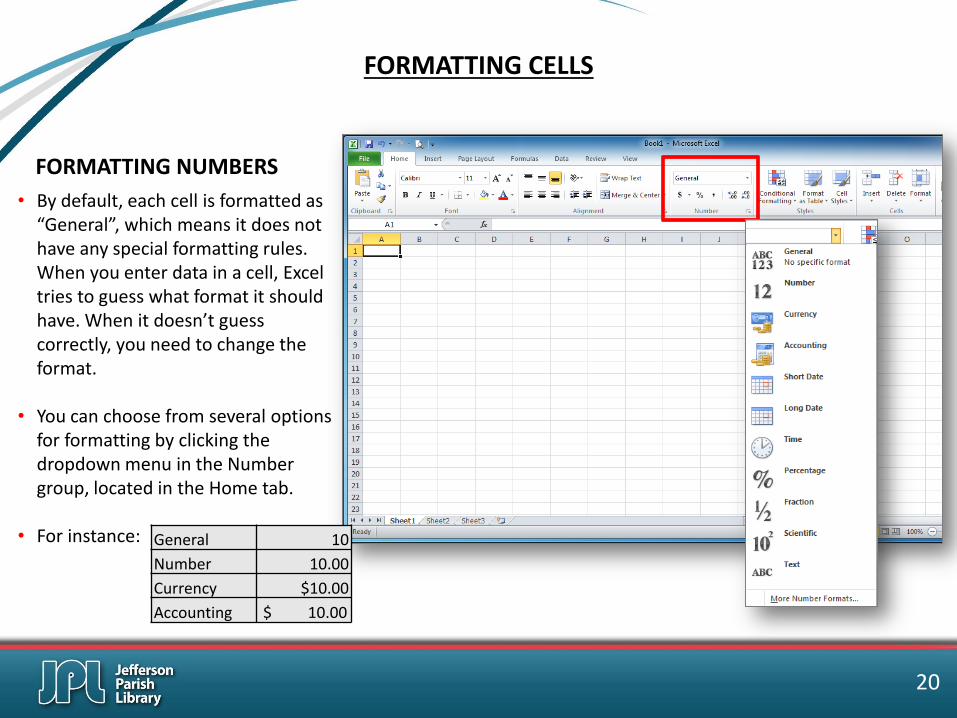
FORMATTING NUMBERS

• By default, each cell is formatted as “General”, which means it does not have any special formatting rules. When you enter data in a cell, Excel tries to guess what format it should have. When it doesn’t guess correctly, you need to change the format.

• You can choose from several options for formatting by clicking the dropdown menu in the Number group, located in the Home tab.

• For instance:

FORMATTING CELLS

General 10

Number 10.00

Currency $10.00

Accounting $ 10.00

20

• There are two different save commands in Excel: SAVE AND SAVE AS

SAVING A WORKBOOK

Save Save As

New File You will be prompted to give the file a name and choose a save location. You can also specify a file type.

You will be prompted to give the file a name and choose a save location. You can also specify a file type.

Existing File Any changes you made will be applied to the existing file in its current location.

You have the option to give the file a new name and/or a new save location. You can also specify a new file type. If you do change something, the original existing file will not be changed.

• Both save commands are found in the File menu:

21

SAVING A WORKBOOK

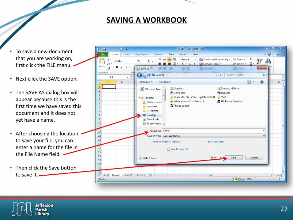
• To save a new document that you are working on, first click the FILE menu.

• Next click the SAVE option.

• The SAVE AS dialog box will appear because this is the first time we have saved this document and it does not yet have a name.

• After choosing the location to save your file, you can enter a name for the file in the File Name field.

• Then click the Save button to save it.

22

MICROSOFT EXCEL EXERCISE

• Open Microsoft Excel. You can double click the Excel icon on the desktop OR

- Go to the START menu - Click ALL PROGRAMS - Scroll down to the Microsoft Office folder and click to open - Click Microsoft Excel • Once the blank document is open, select columns A through E.

- Click and hold down on column A in the upper left corner of your worksheet and then drag your mouse to the right to select column B through E as well.

• Adjust the width of the columns.

- With the cells still highlighted, click Format button in the ribbon (this button is located in the Cells group on the Home tab). Click on ‘Column Width’

OR

- With the cells still highlighted, right-click anywhere in the highlighted area. - From the menu that appears, click on ‘Column Width’. • Change the column width to 17.00

- From the dialog box that appears, simply type in the number 17 and click OK. Continued on next page…

23

MICROSOFT EXCEL EXERCISE

• Now adjust the height of your rows.

- Click and hold down on row 1. - Next, drag your mouse down to row 30 and release your mouse button. Rows 1 through 30 should now be

selected. - With the cells still highlighted, click Format button in the ribbon (this button is located in the Cells group on the

Home tab). Click on ‘Row Height’.

OR

- With the cells still highlighted, right-click anywhere in the highlighted area. - From the menu that appears, click on ‘Row Height’. • Change the row height to 23.00

- From the dialog box that appears, simply type in the number 23 and click OK.

• Type ‘Monthly Expenses’ into cell A1 and tab over to the next cell by pressing the Tab key on your keyboard.

• Underline and Bold the text in cell A1.

- Select cell A1 by clicking on it with your mouse. - Click the B button and then the U button in the Font group located in the Ribbon.

Continued on next page…

24

MICROSOFT EXCEL EXERCISE

• Merge and Center your title.

- Select cells A1 through E1 by clicking and dragging across the cells. - Next click on the Merge & Center button located in the ribbon (this button is in the Alignment group on the

Home tab. • Enter the following data:

- Type the word Groceries in cell B2. - Type the word Utilities in cell C2. - Type the word Insurance in cell D2. - Type the word Recreation in cell E2. - Type the word Total in cell A16. Make the text in this cell bold by clicking the B button in the Ribbon.

• Make a list of the months of the year beginning with January in cell A3. - Begin by typing the word January in cell A3. - Next, use the Autofill function to fill in the rest of the months of the year. Hover your mouse over the small

black square located in the lower left corner of cell A3 until you see cursor change to a black cross. - Next, click and hold down on your mouse and drag down the column. You will see a dialog box populate with

each month as you move down the rows. Release your mouse on row 14. - You should now see January through December listed in Column A.

Continued on next page…

25

MICROSOFT EXCEL EXERCISE

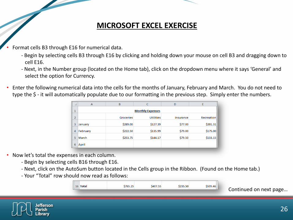
• Format cells B3 through E16 for numerical data.

- Begin by selecting cells B3 through E16 by clicking and holding down your mouse on cell B3 and dragging down to cell E16.

- Next, in the Number group (located on the Home tab), click on the dropdown menu where it says ‘General’ and select the option for Currency.

• Enter the following numerical data into the cells for the months of January, February and March. You do not need to type the $ - it will automatically populate due to our formatting in the previous step. Simply enter the numbers.

• Now let’s total the expenses in each column. - Begin by selecting cells B16 through E16. - Next, click on the AutoSum button located in the Cells group in the Ribbon. (Found on the Home tab.) - Your “Total” row should now read as follows: Continued on next page…

26

MICROSOFT EXCEL EXERCISE

• Your spreadsheet should look like this. You can see what the printed version will look like by clicking on the Print Preview icon in the Quick Access toolbar OR - Click on the File tab - Next, click on the Print option located in the column of options on the left.

• Save your document.

- Click on the File Tab. - Click the Save button. - Choose the Desktop as the location to save your file. - Click in the File Name box to highlight the name that was auto filled. - Type your first and last name and then click the Save button. • Close the program.

27

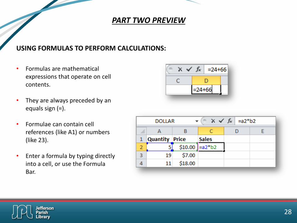
USING FORMULAS TO PERFORM CALCULATIONS:

• Formulas are mathematical expressions that operate on cell contents.

• They are always preceded by an equals sign (=).

• Formulae can contain cell references (like A1) or numbers (like 23).

• Enter a formula by typing directly into a cell, or use the Formula Bar.

PART TWO PREVIEW

28

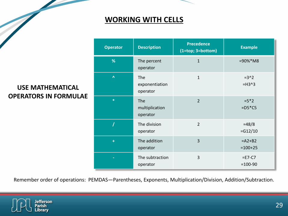
USE MATHEMATICAL OPERATORS IN FORMULAE

Operator Description Precedence

(1=top; 3=bottom) Example

% The percent

operator

1 =90%*M8

^ The

exponentiation

operator

1 =3^2

=H3^3

* The

multiplication

operator

2 =5*2

=D5*C5

/ The division

operator

2 =48/8

=G12/10

+ The addition

operator

3 =A2+B2

=100+25

- The subtraction

operator

3 =E7-C7

=100-90

Remember order of operations: PEMDAS—Parentheses, Exponents, Multiplication/Division, Addition/Subtraction.

WORKING WITH CELLS

29

COMMON KEYBOARD SHORTCUTS

CTRL + A Select entire document/page

CTRL + C Copy selected text/object

CTRL + X Cut selected text/object

CTRL + V Paste selected text/object

CTRL + Z Undo your last action

CTRL + F Find specific text in the current document

CTRL + S Save the current document

CTRL + P Print the current document

CTRL + B Bolds the selected text

CTRL + I Italicizes the selected text

CTRL + U Underlines the selected text

CTRL + N Create a new document

30

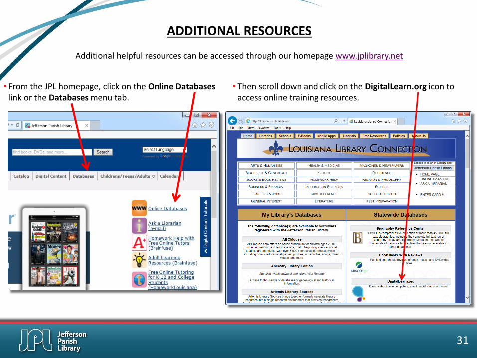
ADDITIONAL RESOURCES

Additional helpful resources can be accessed through our homepage www.jplibrary.net

• From the JPL homepage, click on the Online Databases link or the Databases menu tab.

• Then scroll down and click on the DigitalLearn.org icon to access online training resources.

31

ADDITIONAL RESOURCES

Additional helpful resources can be accessed through our homepage www.jplibrary.net

• From the library’s homepage, click on the JPL Digital Content link or the Digital Content menu tab.

• Then click on the lynda.com icon to access online training using your library card number and pin.

32

NOTES

Jefferson Parish Library authorizes you to view and download materials such as this handout at our web site (www.jefferson.lib.la.us) only for your personal, non-commercial use, provided that you retain all copyright and other proprietary notices contained in the original materials on all copies of the materials. You may not modify the materials at this site in any way or reproduce, publicly display, perform, distribute or otherwise use them for any public or commercial purpose. The materials at this

site are copyrighted and any unauthorized use of any materials at this site may violate copyright, trademark, and other laws. If you breach any of these Terms, your authorization to use any materials available at this site automatically terminates and you must immediately destroy any such downloaded or printed materials.

33