Basic Concepts and Theorems of Structural Analysis · BASIC CONCEPTS AND THEOREMS OF STRUCTURAL...

CHAPTER 1

Basic Concepts and Theorems of Structural Analysis

1.1 INTRODUCTION

In this chapter, basic definitions, concepts and theorems of structural analysis are presented. These theorems are employed in the following chapters and are very important for their understanding.

For an analytical determination of the distribution of internal forces and displace-ments, under prescribed external loading, a solution to the basic equations of the theory of structures should be obtained, satisfying the boundary conditions. In the matrix methods of structural analysis, one must also use these basic equations.

In order to provide a ready reference for the development of the general theory of matrix structural analysis, the most important basic theorems are introduced in this chapter, and illustrated through simple examples.

1.1.1 DEFINITIONS

A structure can be defined as a body that resists external effects (loads, tempera-ture changes and support settlements) without undue deformation. Building frames, industrial building, halls, towers, bridges, dams, reservoirs, tanks, channels and pavements are typical structures that are of interest to civil engineers. _________________________________ Optimal Structural Analysis A. Kaveh © 2006 Research Studies Press Limited

COPYRIG

HTED M

ATERIAL

OPTIMAL STRUCTURAL ANALYSIS

2

The underlying principles for the analysis of other structures are more or less the same. Airplane, missile and satellite structures are of interest to the aviation engi-neer. The analysis and design of a ship is interesting for a naval architect. A machine engineer should be able to design machine parts. However, in this book only structures that are of interest to structural engineers will be studied.

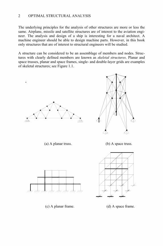
A structure can be considered to be an assemblage of members and nodes. Struc-tures with clearly defined members are known as skeletal structures. Planar and space trusses, planar and space frames, single- and double-layer grids are examples of skeletal structures; see Figure 1.1.

(a) A planar truss. (b) A space truss.

(c) A planar frame. (d) A space frame.

BASIC CONCEPTS AND THEOREMS OF STRUCTURAL ANALYSIS

3

(e) A single-layer grid. (f) A double-layer grid.

Fig. 1.1 Examples of skeletal structures.

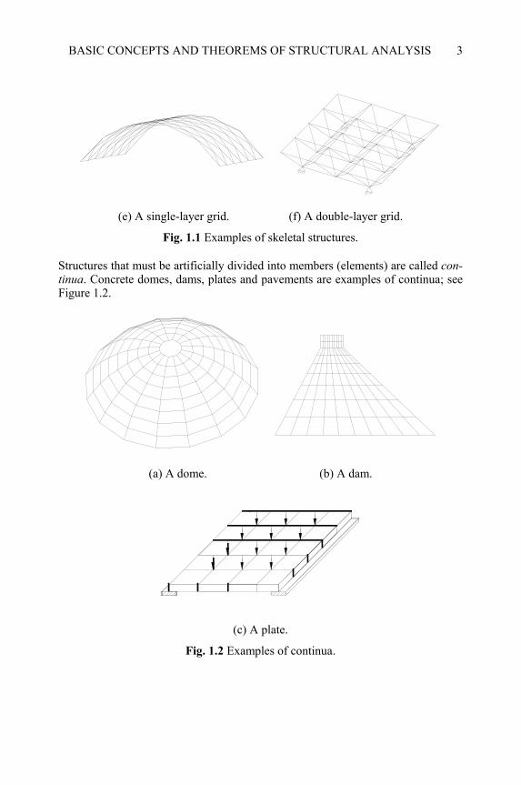
Structures that must be artificially divided into members (elements) are called con-tinua. Concrete domes, dams, plates and pavements are examples of continua; see Figure 1.2.

(a) A dome. (b) A dam.

(c) A plate.

Fig. 1.2 Examples of continua.


4

1.1.2 STRUCTURAL ANALYSIS AND DESIGN

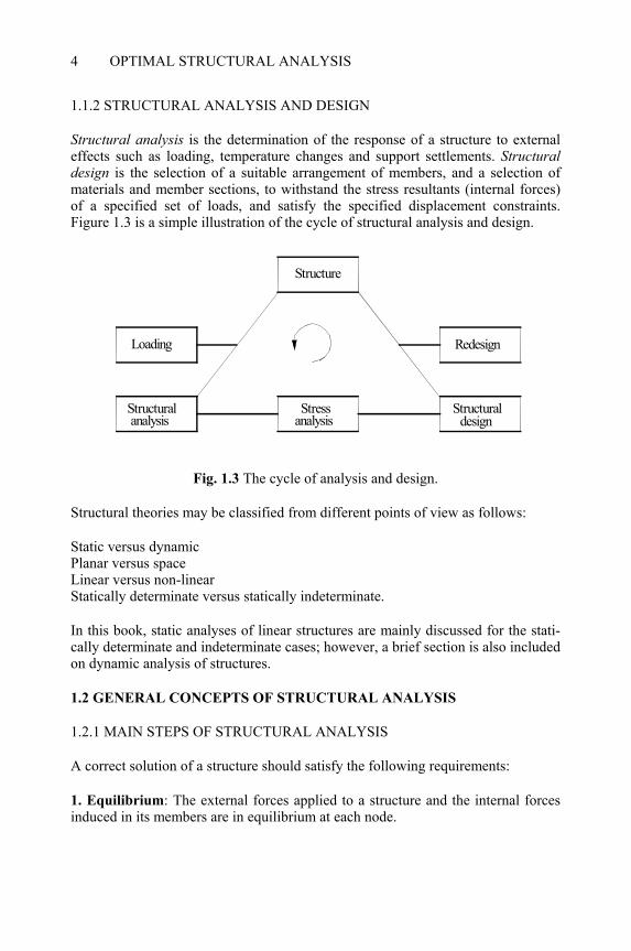
Structural analysis is the determination of the response of a structure to external effects such as loading, temperature changes and support settlements. Structural design is the selection of a suitable arrangement of members, and a selection of materials and member sections, to withstand the stress resultants (internal forces) of a specified set of loads, and satisfy the specified displacement constraints. Figure 1.3 is a simple illustration of the cycle of structural analysis and design.

Fig. 1.3 The cycle of analysis and design.

Structural theories may be classified from different points of view as follows:

Static versus dynamic Planar versus space Linear versus non-linear Statically determinate versus statically indeterminate.

In this book, static analyses of linear structures are mainly discussed for the stati-cally determinate and indeterminate cases; however, a brief section is also included on dynamic analysis of structures.

1.2 GENERAL CONCEPTS OF STRUCTURAL ANALYSIS

1.2.1 MAIN STEPS OF STRUCTURAL ANALYSIS

A correct solution of a structure should satisfy the following requirements:

1. Equilibrium: The external forces applied to a structure and the internal forces induced in its members are in equilibrium at each node.

Structure

Structural analysis Structural

design

Loading Redesign

Stress analysis


5

2. Compatibility: The members should deform so that they fit together.

3. Force–displacement relationship: The internal forces and deformations satisfy the stress–strain relationship of the member.

For structural analysis, two basic methods are in use:

Force method: In this method, some of the internal forces and/or reactions are taken as primary unknowns, called redundants. Then the stress–strain relationship is used to express the deformations of the members in terms of external and redun-dant forces. Finally, by applying the compatibility condition that the deformed members must fit together, a set of linear equations yields the values of the redun-dant forces. The stresses in the members are then calculated and the displacements at the nodes in the direction of external forces are found. This method is also known as the flexibility method and compatibility approach.

Displacement method: In this method, the displacements of the nodes necessary to describe the deformed state of the structure are taken as unknowns. The defor-mations of the members are then calculated in terms of these displacements, and by using the stress–strain relationship, the internal forces are related to them. Finally, by applying the equilibrium equations at each node, a set of linear equations is obtained, the solution of which results in the unknown nodal displacements. This method is also known as the stiffness method and equilibrium approach.

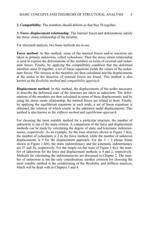
For choosing the most suitable method for a particular structure, the number of unknowns is one of the main criteria. A comparison of the force and displacement methods can be made by calculating the degree of static and kinematic indetermi-nacies, respectively. As an example, for the truss structure shown in Figure 1.4(a), the number of redundants is 2 in the force method, while the number of unknown displacements is 9 for the displacement approach. For the 3 × 3 planar frame shown in Figure 1.4(b), the static indeterminacy and the kinematic indeterminacy are 27 and 36, respectively. For the simple six-bar truss of Figure 1.4(c), the num-ber of unknowns for the force and displacement methods is 4 and 2, respectively. Methods for calculating the indeterminacies are discussed in Chapter 2. The num-ber of unknowns is not the only consideration: another criterion for choosing the most suitable method is the conditioning of the flexibility and stiffness matrices, which will be dealt with in Chapters 3 and 4.


6

(a) A planar truss. (b) A planar frame. (c) A simple truss.

Fig. 1.4 Some simple structures.

1.2.2 MEMBER FORCES AND DISPLACEMENTS

A structure can be considered as an assembly of its members, subject to external effects. These effects will be considered as external loads applied at nodes, since any other effect can be reduced to such equivalent nodal loads. The state of stress in a member (internal forces) is defined by a vector,

t1 2 3{ ... }k k k k

m nr r r r=r , (1-1)

and the associated member deformation (distortion) is designated by a vector,

t1 2 3{ ... } ,k k k k

m nu u u u=u (1-2)

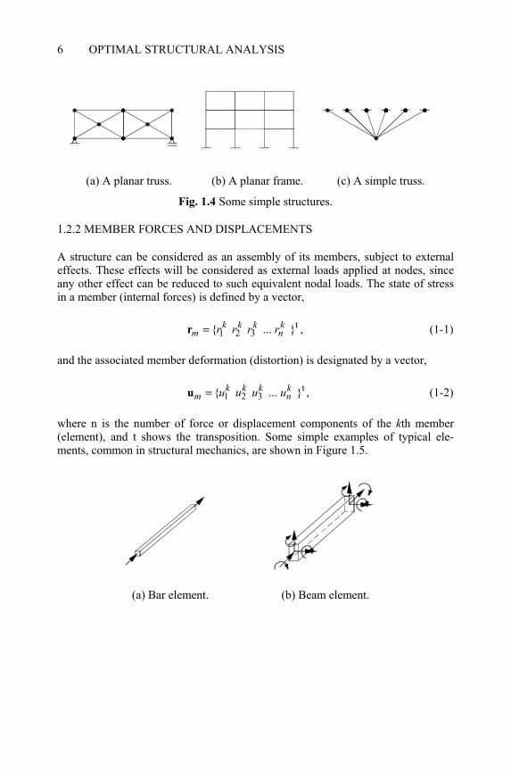
where n is the number of force or displacement components of the kth member (element), and t shows the transposition. Some simple examples of typical ele-ments, common in structural mechanics, are shown in Figure 1.5.

(a) Bar element. (b) Beam element.


7

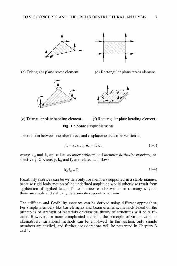
(c) Triangular plane stress element. (d) Rectangular plane stress element.

(e) Triangular plate bending element. (f) Rectangular plate bending element.

Fig. 1.5 Some simple elements.

The relation between member forces and displacements can be written as

rm = kmum or um = fmrm, (1-3)

where km and fm are called member stiffness and member flexibility matrices, re-spectively. Obviously, km and fm are related as follows:

kmfm = I. (1-4)

Flexibility matrices can be written only for members supported in a stable manner, because rigid body motion of the undefined amplitude would otherwise result from application of applied loads. These matrices can be written in as many ways as there are stable and statically determinate support conditions.

The stiffness and flexibility matrices can be derived using different approaches. For simple members like bar elements and beam elements, methods based on the principles of strength of materials or classical theory of structures will be suffi-cient. However, for more complicated elements the principle of virtual work or alternatively variational methods can be employed. In this section, only simple members are studied, and further considerations will be presented in Chapters 3 and 4.


8

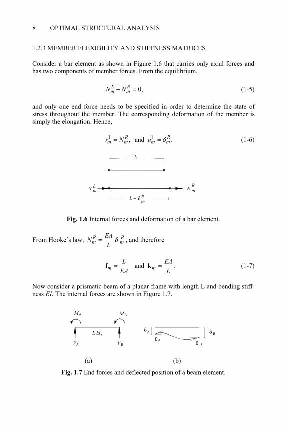
1.2.3 MEMBER FLEXIBILITY AND STIFFNESS MATRICES

Consider a bar element as shown in Figure 1.6 that carries only axial forces and has two components of member forces. From the equilibrium,

0,L Rm mN N+ = (1-5)

and only one end force needs to be specified in order to determine the state of stress throughout the member. The corresponding deformation of the member is simply the elongation. Hence,

1 1, and .R Rm m m mr N u δ= = (1-6)

Fig. 1.6 Internal forces and deformation of a bar element.

From Hooke´s law, R Rm m

EANL

δ= , and therefore

and .m mL EA

EA L= =f k (1-7)

Now consider a prismatic beam of a planar frame with length L and bending stiff-ness EI. The internal forces are shown in Figure 1.7.

M M

V V A B

A B L, E I z A A

B B δ δ θ

θ

(a) (b)

Fig. 1.7 End forces and deflected position of a beam element.

L N

R

L

L

N R

m m m + δ


9

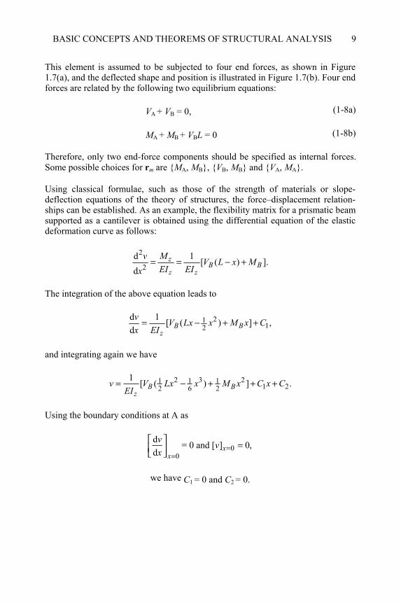
This element is assumed to be subjected to four end forces, as shown in Figure 1.7(a), and the deflected shape and position is illustrated in Figure 1.7(b). Four end forces are related by the following two equilibrium equations:

VA + VB = 0, (1-8a)

MA + MB + VBL = 0 (1-8b)

Therefore, only two end-force components should be specified as internal forces. Some possible choices for rm are {MA, MB}, {VB, MB} and {VA, MA}.

Using classical formulae, such as those of the strength of materials or slope-deflection equations of the theory of structures, the force–displacement relation-ships can be established. As an example, the flexibility matrix for a prismatic beam supported as a cantilever is obtained using the differential equation of the elastic deformation curve as follows:

2

2d 1 [ ( ) ].d

zB B

z z

Mv V L x MEI EIx

= = − +

The integration of the above equation leads to

2112

d 1 [ ( ) ] ,d B B

z

v V Lx x M x Cx EI

= − + +

and integrating again we have

2 3 21 1 11 22 6 2

1 [ ( ) ] .B Bz

v V Lx x M x C x CEI

= − + + +

Using the boundary conditions at A as

00

d = 0 and [ ] 0,d =

=

= x

x

v vx

we have C1 = 0 and C2 = 0.


10

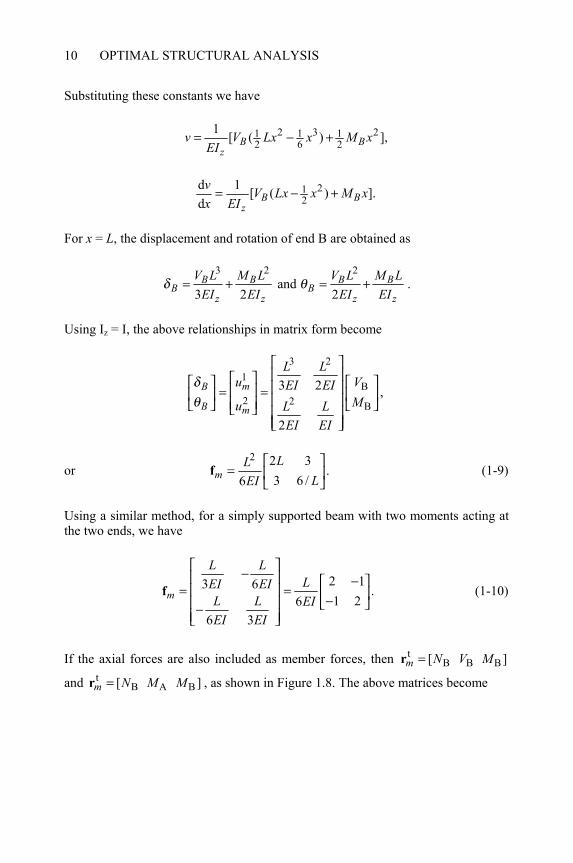
Substituting these constants we have

2 3 21 1 12 6 2

1 [ ( ) ],B Bz

v V Lx x M xEI

= − +

212

d 1 [ ( ) ].d B B

z

v V Lx x M xx EI

= − +

For x = L, the displacement and rotation of end B are obtained as

3 2 2 and

3 2 2B B B B

B Bz z z z

V L M L V L M LEI EI EI EI

δ θ= + = + .

Using Iz = I, the above relationships in matrix form become

3 21

B2 2 B

3 2 ,

2

mB

B m

L Lu VEI EI

Mu L LEI EI

δθ

= =

or 2 2 3

.3 6 /6mLL

LEI

=

f (1-9)

Using a similar method, for a simply supported beam with two moments acting at the two ends, we have

2 13 6 .1 26

6 3

m

L LLEI EI

L L EIEI EI

− − = = − −

f (1-10)

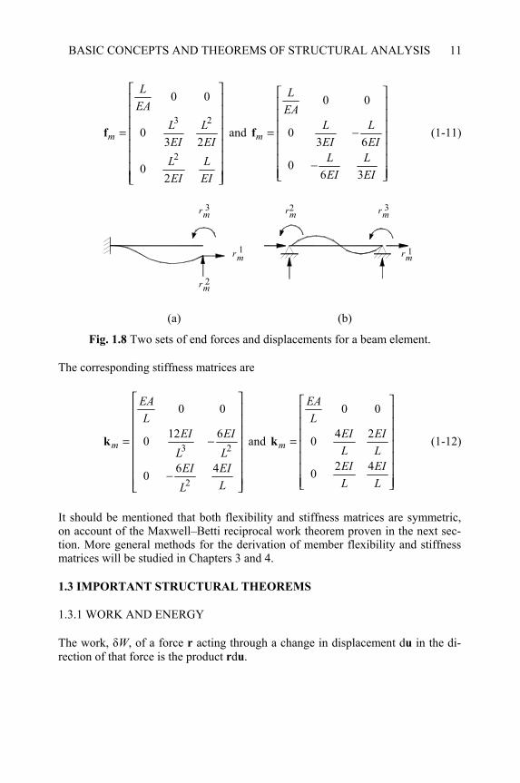
If the axial forces are also included as member forces, then tB B B[ ]m N V M=r

and tB A B[ ]m N M M=r , as shown in Figure 1.8. The above matrices become


11

3 2

2

0 0

03 2

02

m

LEA

L LEI EIL LEI EI

=

f and

0 0

03 6

06 3

m

LEA

L LEI EIL LEI EI

= − −

f (1-11)

3 m r m r m r

m r m r

m r 1 2 3

2 1

(a) (b)

Fig. 1.8 Two sets of end forces and displacements for a beam element.

The corresponding stiffness matrices are

3 2

2

0 0

12 60

6 40

m

EAL

EI EIL L

EI EILL

= −

−

k and

0 0

4 20

2 40

m

EAL

EI EIL LEI EIL L

=

k (1-12)

It should be mentioned that both flexibility and stiffness matrices are symmetric, on account of the Maxwell–Betti reciprocal work theorem proven in the next sec-tion. More general methods for the derivation of member flexibility and stiffness matrices will be studied in Chapters 3 and 4.

1.3 IMPORTANT STRUCTURAL THEOREMS

1.3.1 WORK AND ENERGY

The work, δW, of a force r acting through a change in displacement du in the di-rection of that force is the product rdu.


12

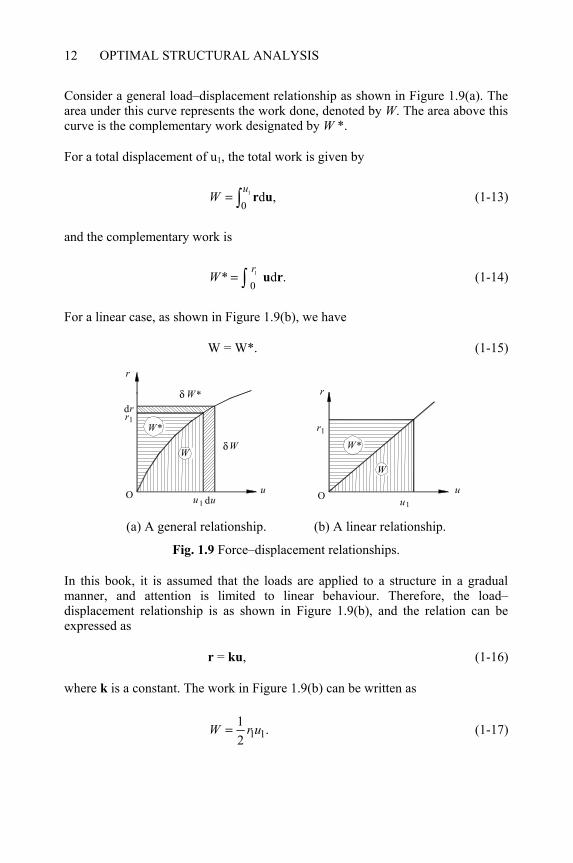
Consider a general load–displacement relationship as shown in Figure 1.9(a). The area under this curve represents the work done, denoted by W. The area above this curve is the complementary work designated by W *.

For a total displacement of u1, the total work is given by

1

0d ,

uW = ∫ r u (1-13)

and the complementary work is

1 0

* d .r

W = ∫ u r (1-14)

For a linear case, as shown in Figure 1.9(b), we have

W = W*. (1-15)

δ

r r

u u W

W

W

W * W * W *

u u

r

1

d r

d u 1

1 r 1

O O

δ

(a) A general relationship. (b) A linear relationship.

Fig. 1.9 Force–displacement relationships.

In this book, it is assumed that the loads are applied to a structure in a gradual manner, and attention is limited to linear behaviour. Therefore, the load–displacement relationship is as shown in Figure 1.9(b), and the relation can be expressed as

r = ku, (1-16)

where k is a constant. The work in Figure 1.9(b) can be written as

1 11 .2

W r u=

(1-17)


13

Forces and displacements at a point are both represented by vectors, and their work is represented as a dot product. In matrix notations, however, the work can be written as

t1 .2

W = r u (1-18)

Using Eq. (1-3),

t t t1 1 .

2 2W = =u k u u ku

(1-19)

Similarly, W * can be calculated as

t1* .2

W = r fr (1-20)

Consider the stress–strain relationship as illustrated in Figure 1.10(a). The area under this curve represents the density of the strain energy, and when integrated over the volume of the member (or structure) results in the strain energy U. The area to the left of the stress–strain curve is the density of the complementary strain energy, and by integrating over the member (or structure) the complementary en-ergy U* is obtained. For the linear stress–strain relationship as shown in Figure 1.10(b), U = U*.

Since the work done by external actions on an elastic system is equal to the strain energy stored internally in the system (work-energy law),

W = U and W* = U*. (1-21)

U U

U * U *

O O

σ σ

ε ε

(a) A general stress–strain relationship. (b) Linear stress–strain relationship.

Fig. 1.10 Stress–strain relationships.


14

1.3.2 CASTIGLIANO´S THEOREMS

Consider the force–displacement curve in Figure 1.9(a), and suppose an imaginary displacement δui is imposed on the system. The work done, δ ,W under the action of ri in moving through δ iu is equal to

δ .i iW r uδ = (1-22)

Using Eq. (1-21), and taking limit, we get the first theorem of Castigliano as

,ii

U rq

∂ =∂

(1-23)

which can be stated as follows [24]:

The partial derivative of the strain energy with respect to a dis-placement is equal to the force applied at the point and along the considered displacement.

Similarly, if the system is subjected to an imaginary force irδ along the displace-ment ui, then the complementary work done *δW is equal to

* *,δ δ δ= =i iW u r U (1-24)

and in the limit, the second theorem of Castigliano is obtained as

* .ii

U ur

∂ =∂

(1-25)

The partial derivative of the complementary strain energy with re-spect to a force is equal to the displacement at the point where the force is applied and directed along the action of the force.

For the linear case, * =U U and therefore Eq. (1-25) becomes

.ii

U ur

∂ =∂

(1-26)


15

1.3.3 PRINCIPLE OF VIRTUAL WORK The principle of virtual work is a very powerful means for deducing the conditions of compatibility and equilibrium [5], and it can be stated as follows: The work done by a set of external forces P acting on a structure in moving through the associated displacements v, is equal to the work done by some other set of forces R, that is statically equivalent to P, moving through associated dis-placements u, that are compatible with v. Associated forces and displacements have the same lines of actions. Using a statically admissible set of forces and the work equation, the compatibility relations between the deformations and displacements can be derived. Alterna-tively, employing a compatible set of displacements and the work equation, one obtains the equations of equilibrium between the forces. These approaches are elegant and practical. Dummy-Load Theorem: This theorem can be used to determine the conditions of compatibility. Suppose that the deformed shape of each member of a structure is known. Then it is possible to find the deflection of the structure at any point by using the principle of virtual work. For this purpose, a dummy load (usually unit load) is applied at the point and in the direction of required displacement, which is why it is also known as the unit load method. The dummy-load theorem can be stated as follows:

applied actual displacement internal forces actualdummy of structure where external statically equivalent to deformationload dummy load is applied the applied dummy load of ele

× = × ments

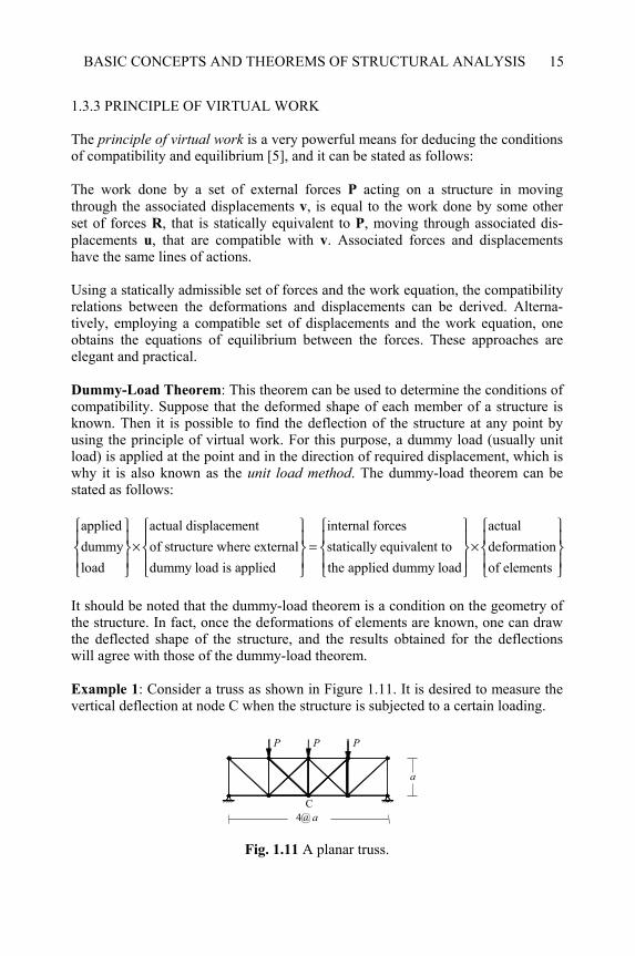
It should be noted that the dummy-load theorem is a condition on the geometry of the structure. In fact, once the deformations of elements are known, one can draw the deflected shape of the structure, and the results obtained for the deflections will agree with those of the dummy-load theorem. Example 1: Consider a truss as shown in Figure 1.11. It is desired to measure the vertical deflection at node C when the structure is subjected to a certain loading.

4@ a a

P P P

C

Fig. 1.11 A planar truss.


16

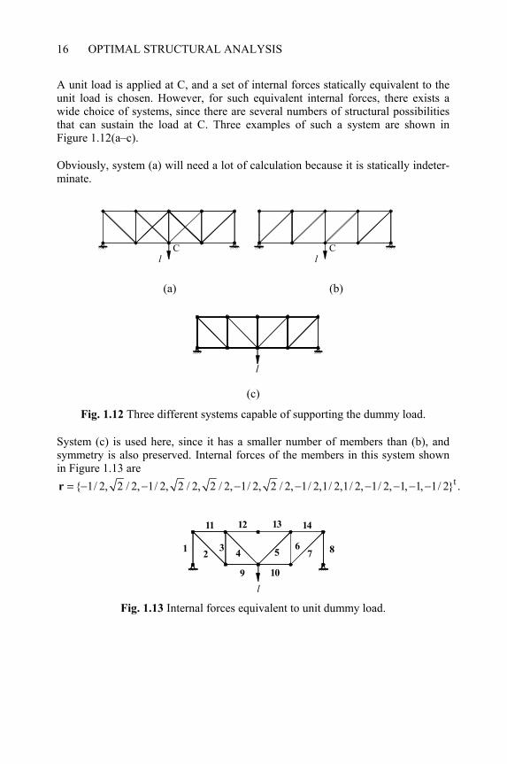
A unit load is applied at C, and a set of internal forces statically equivalent to the unit load is chosen. However, for such equivalent internal forces, there exists a wide choice of systems, since there are several numbers of structural possibilities that can sustain the load at C. Three examples of such a system are shown in Figure 1.12(a–c).

Obviously, system (a) will need a lot of calculation because it is statically indeter-minate.

C l C

l

(a) (b)

l (c)

Fig. 1.12 Three different systems capable of supporting the dummy load.

System (c) is used here, since it has a smaller number of members than (b), and symmetry is also preserved. Internal forces of the members in this system shown in Figure 1.13 are

t{ 1/ 2, 2 / 2, 1/ 2, 2 / 2, 2 / 2, 1/ 2, 2 / 2, 1/ 2,1/ 2,1/ 2, 1/ 2, 1, 1, 1/ 2} .= − − − − − − − −r

l

1 2 3 4 5 6 7 8

9 10 11 12 13 14

Fig. 1.13 Internal forces equivalent to unit dummy load.


17

Measuring the elongation in members of this system containing 14 bars, and using the dummy-load theorem, we have

1 2 3 4 5 6

7 8 9 10 11 12 13 14

1 1 1 2 1 2 2 1( )(0) (1)( ) ( )(0)2 2 2 2 2 2 2 2

2 1 1 1 1 1 .2 2 2 2 2 2

c cv v e e e e e e

e e e e e e e e

+ + = = − + + − + + −

+ − + + − − − −

Dummy-Displacement Theorem: This method is usually used to find the applied external forces when the internal forces are known. In order to obtain the external force at a particular point, one subjects the structure to a unit displacement at that point in the direction of the force and chooses any set of deformations compatible with the unit displacement. Then, from the principle of work, the dummy-displacement theorem can be stated as follows:

dummy displacement applied actual deformation of elements actualin the direction of unknowns external compatible with internalactual external forces forces dummy displacement f

× = × orces

This method is also known as the unit displacement method.

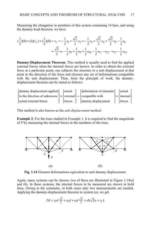
Example 2: For the truss studied in Example 1, it is required to find the magnitude of P by measuring the internal forces in the members of the truss.

r C d d

C

r r r

P

2 1 1 2

(a) (b)

Fig. 1.14 Element deformations equivalent to unit dummy displacement.

Again, many systems can be chosen; two of these are illustrated in Figure 1.14(a) and (b). In these systems, the internal forces to be measured are shown in bold lines. Owing to the symmetry, in both cases only two measurements are needed. Applying the dummy-displacement theorem to system (a), we get

2 21 2 1 1 22 2 ( 2 ).Pd r d r d r d d r r= + + = +


18

1.3.4 CONTRAGRADIENT PRINCIPLE

Consider two statically equivalent force systems R and P related by a linear trans-formation as

R = BP, (1-27)

R is considered to have more entries than P, that is, there are solutions to R for which P is zero. Associated with R and P let there be two sets of displacements v and u, respectively. These are compatible displacements and therefore the work done in each system is the same, that is,

Ptu = Rtv. (1-28)

From Eq. (1-27),

Rt = PtBt. (1-29)

Therefore,

Ptu = PtBtv. (1-30)

Since P is arbitrary, we have

u = Btv. (1-31)

Equations (1-27) and (1-31) will be used in the formulation of the force method.

In a general structure, if member forces R are related to external nodal loads P, similar to Eq. (1-27), then according to the contragradient principle [5], the mem-ber distortions v and nodal displacement u will be related by an equation similar to Eq. (1-31).

If two displacement systems u and v are related by a linear transformation as

v = Cu, (1-32)

and R and P are statically equivalent forces, then equating the work done for com-patible displacements we have

Ptu = Rtv = RtCu. (1-33)

Again u is arbitrary and

P = CtR. (1-34)


19

Equations (1-32) and (1-34) are employed in the formulation of the displacement method.

For a statically determinate structure,

1 ,−=P B R (1-35)

and therefore

t 1.−=C B (1-36)

1.3.5 RECIPROCAL WORK THEOREM

Consider a structure as shown in Figure 1.15(a) subjected to a set of loads, {P1, P2, … , Pm}. The same structure is considered under the action of a second set of loads {Q1, Q2, … , Qn}, as shown in Figure 1.15(b). The reciprocal work theorem can be stated as follows:

The work done by {P1, P2, … , Pm} through displacements {δ1, δ2, … , δm} produced by {Q1, Q2, … , Qn} is the same as the work done by {Q1, Q2, … , Qn} through displacements {∆1, ∆2, … , ∆n} produced by {P1, P2, … , Pm}; that is,

1 1

m n

i i j ji j

P Qδ= =

= ∆∑ ∑ . (1-37)

When single loads P and Q are considered, Eq. (1-37) reduces to

,i jP Qδ = ∆ (1-38)

and for the case where P = Q, one obtains

.i jδ = ∆ (1-39)

Equation (1-39) is known as Betti´s law, and can be stated as follows:

The deflection at point i due to a load at point j is the same as deflection at j when the same load is applied at i.


20

∆ ∆

∆ ∆

δ δ δ P

P

P

Q Q

Q

Q

1 2

m 1

2 2 1 1

2 3

n n m

(a) (b)

Fig. 1.15 A structure subjected to two sets of loads.

The proof of the reciprocal work theorem is constructed by equating the strain energy of the structure in two different loading sequences [217]. In the first se-quence, both sets of loads are applied simultaneously, while in the second sequence, loads {P1, P2, … , Pm} are applied first, followed by the application of the second set of loads {Q1, Q2, … , Qn}.

EXERCISES

1.1 Using slope-deflection equations, write the stiffness matrix for a prismatic beam.

1.2 Develop the flexibility matrix for a beam element, using simple supports for the element.

1.3 Show that the alternative forms of the beam flexibility matrices yield the same complementary energy.

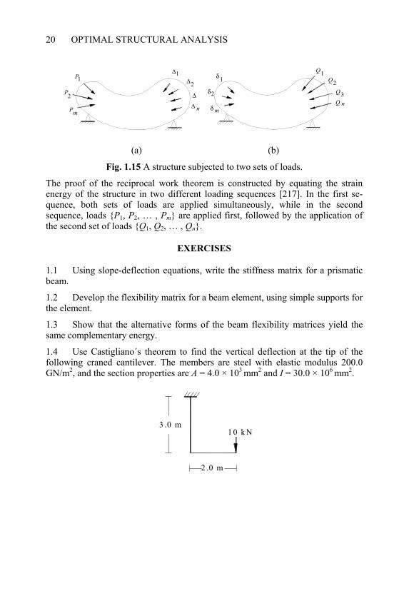
1.4 Use Castigliano´s theorem to find the vertical deflection at the tip of the following craned cantilever. The members are steel with elastic modulus 200.0 GN/m2, and the section properties are A = 4.0 × 103 mm2 and I = 30.0 × 106 mm2.

3 .0 m

2 .0 m

1 0 k N


21

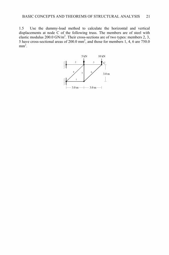
1.5 Use the dummy-load method to calculate the horizontal and vertical displacements at node C of the following truss. The members are of steel with elastic modulus 200.0 GN/m2. Their cross-sections are of two types: members 2, 3, 5 have cross-sectional areas of 200.0 mm2, and those for members 1, 4, 6 are 750.0 mm2.

3.0 m 3.0 m 3.0 m

10 kN 5 kN

1

2 3 4 5 6

C

Basic Concepts and Theorems of Structural Analysis · BASIC CONCEPTS AND THEOREMS OF STRUCTURAL...

Documents

Transcript of Basic Concepts and Theorems of Structural Analysis · BASIC CONCEPTS AND THEOREMS OF STRUCTURAL...