Basic and Advanced Database Courses - u-szeged.hu · Basic and Advanced Database ... some basic...

Basic and Advanced DatabaseCoursesSrdjan Skrbic

Faculty of Science, University of Novi SadTrg Dositeja Obradovica 4, 21000 Novi Sad, Serbia

[email protected]://www.is.pmf.uns.ac.rs/skrbics

At the beginning of the course, we explore some basic database concepts and adopt terminology. We give an overviewof the most important data models. First we give brief remarks on historical network and hierarchical data models, andthen we continue to investigate entity-relationship and relational data model. Only most important facts about entity-relationship model, together with some examples will be covered. The relational data model will be presented in muchmore detail, but we concentrate on exploring possibilities for its practical usage. Important remarks about theoreticalbackground of the relational model are covered later in the text. We continue with the most important constructions ofthe Structured Query Language.In the advanced level course, we concentrate on the theoretical background of the relational model, explore it in somedetail, and explain implications these concepts make to the usage of the relational model in practice. Among othertopics, we explore functional dependencies in detail. Next, we give some pointers on update anomalies and the need tointroduce normal (canonical) forms to relational database theory. We describe normal forms from first to third, includingthe Boyce-Codd normal form that belongs somewhere between the third and the fourth. We also give pointers aboutother normal forms. At the end we introduce two algorithms for relational database normalization - decomposition andsynthesis.

1. Introduction

Databases today are essential to every business. Whenever you visit a major Web site Google, Yahoo!, Ama-zon.com, or thousands of smaller sites that provide information there is a database behind the scenes servingup the information you request. Corporations maintain all their important records in databases. Databases arelikewise found at the core of many scientific investigations. They represent the data gathered by astronomers,by investigators of the human genome, and by biochemists exploring properties of proteins, among many otherscientific activities. The power of databases comes from a body of knowledge and technology that has developedover several decades and is embodied in specialized software called a database management system, or DBMS.A DBMS is a powerful tool for creating and managing large amounts of data efficiently and allowing it to persistover long periods of time, safely. These systems are among the most complex types of software available.

In essence a database is nothing more than a collection of information that exists over a long period of time. Theterm database also refers to a collection of data that is managed by a DBMS. The DBMS is expected to allow usersto:

• create new databases and specify their schemas,

• query the data and modify the data,

• support the storage of very large amounts of data,

2 S. Skrbic

• enable durability, the recovery of the database in the face of failures and

• control access to data from many users at once, without allowing unexpected interactions among users andwithout actions on the data to be performed partially but not completely.

The early DBMS’s required the programmer to visualize data much as it was stored. These database systems usedseveral different data models for describing the structure of the information in a database. Two most importantmodels were ”hierarchical” or tree-based model and the graph-based ”network” model. A problem with these earlymodels and systems was that they did not support high-level query languages. That is why there was considerableeffort needed to write such programs, even for very simple queries.

Following a famous paper written by Codd [3] in 1970, database systems changed significantly. Codd proposedthat database systems should present the user with a view of data organized as tables called relations. Behind thescenes, there might be a complex data structure that allowed rapid response to a variety of queries. But, unlike theprogrammers for earlier database systems, the programmer of a relational system would not be concerned with thestorage structure. Queries could be expressed in a very high-level language, which greatly increased the efficiencyof database programmers.

By 1990, relational database systems were the norm. Yet the database field continues to evolve, and new issues andapproaches to the management of data surface regularly. Object-oriented features have infiltrated the relationalmodel. Some of the largest databases are organized rather differently from those using relational methodology.

1.1. Overview of a Database Management System

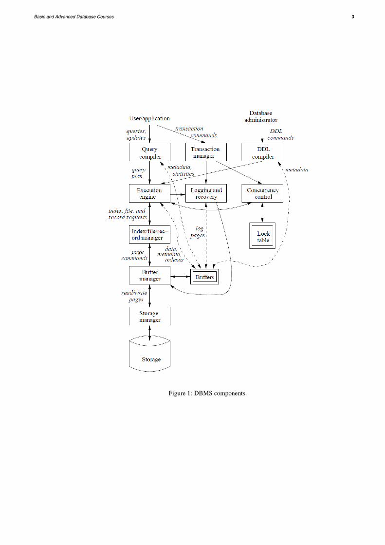
In Fig. 1 we see an outline of a complete DBMS. Single boxes represent system components, while double boxesrepresent in-memory data structures. The solid lines indicate control and data flow, while dashed lines indicatedata flow only. Since the diagram is complicated, we shall consider the details in several stages. First, at the top,we suggest that there are two distinct sources of commands to the DBMS:

1. Conventional users and application programs that ask for data or modify data.

2. A database administrator: a person or persons responsible for the structure or schema of the database.

1.1.1. Query Processing

The second kind of command is the simpler to process, and we show its trail beginning at the upper right side ofFig. 1. For example, the database administrator, or DBA, for a university registrar’s database might decide thatthere should be a table or relation with columns for a student, a course the student has taken, and a grade for thatstudent in that course. The DBA might also decide that the only allowable grades are A, B, C, D, and F. Thisstructure and constraint information is all part of the schema of the database. It is shown in Fig. 1 as enteredby the DBA, who needs special authority to execute schema-altering commands, since these can have profoundeffects on the database. These schema-altering data-definition language (DDL) commands are parsed by a DDLprocessor and passed to the execution engine, which then goes through the index/file/record manager to alter themeta data, that is, the schema information for the database.

The great majority of interactions with the DBMS follow the path on the left side of Fig. 1. A user or an applicationprogram initiates some action, using the data-manipulation language (DML). This command does not affect theschema of the database, but may affect the content of the database or will extract data from the database.

The query is parsed and optimized by a query compiler. The resulting query plan, or sequence of actions the DBMSwill perform to answer the query, is passed to the execution engine. The execution engine issues a sequence ofrequests for small pieces of data, typically records or tuples of a relation, to a resource manager that knows aboutdata files (holding relations), the format and size of records in those files, and index files, which help find elementsof data files quickly.

Basic and Advanced Database Courses 3

Figure 1: DBMS components.

4 S. Skrbic

The requests for data are passed to the buffer manager. The buffer manager’s task is to bring appropriate portionsof the data from secondary storage (disk) where it is kept permanently, to the main-memory buffers. Normally, thepage or ”disk block” is the unit of transfer between buffers and disk.

The buffer manager communicates with a storage manager to get data from disk. The storage manager might in-volve operating-system commands, but more typically, the DBMS issues commands directly to the disk controller.

Queries and other DML actions are grouped into transactions, which are units that must be executed atomicallyand in isolation from one another. Any query or modification action can be a transaction by itself. In addition, theexecution of transactions must be durable, meaning that the effect of any completed transaction must be preservedeven if the system fails in some way right after completion of the transaction.

1.1.2. Storage and Buffer Management

The data of a database normally resides in secondary storage - a magnetic disk, for example. However, to performany useful operation on data, that data must be in main memory. It is the job of the storage manager to control theplacement of data on disk and its movement between disk and main memory. For efficiency purposes, DBMS’snormally control storage on the disk directly, at least under some circumstances. The storage manager keeps trackof the location of files on the disk and obtains the block or blocks containing a file on request from the buffermanager.

The buffer manager is responsible for partitioning the available main memory into buffers, which are page-sizedregions into which disk blocks can be transferred. Thus, all DBMS components that need information from thedisk will interact with the buffers and the buffer manager, either directly or through the execution engine. Thekinds of information that various components may need include: data, meta data, log records, statistics, indexes,etc.

1.1.3. Transaction Processing

It is normal to group one or more database operations into a transaction, which is a unit of work that must beexecuted atomically and in apparent isolation from other transactions. In addition, a DBMS offers the guarantee ofdurability: that the work of a completed transaction will never be lost. The transaction manager therefore acceptstransaction commands from an application, which tell the transaction manager when transactions begin and end,as well as information about the expectations of the application.

The transaction processor performs the following tasks:

1. Logging: In order to assure durability, every change in the database is logged separately on disk.

2. Concurrency control: The concurrency-control manager must assure that the individual actions of multipletransactions are executed in such an order that the net effect is the same as if the transactions had in factexecuted in their entirety, one-at-a-time.

3. Deadlock resolution: As transactions compete for resources through the locks that the scheduler grants,they can get into a situation where none can proceed because each needs something another transaction has.The transaction manager has the responsibility to intervene and cancel (”rollback” or ”abort”) one or moretransactions to let the others proceed.

Properly implemented transactions are commonly said to meet the ”ACID test”, where:

• ”A” stands for ”atomicity,” the all-or-nothing execution of transactions.

• ”C,” stands for ”consistency.” That is, all databases have consistency constraints, or expectations aboutrelationships among data elements.

• ”I” stands for ”isolation,” the fact that each transaction must appear to be executed as if no other transactionis executing at the same time.


• ”D” stands for ”durability,” the condition that the effect on the database of a transaction must never be lost,once the transaction has completed.

1.1.4. The Query Processor

The portion of the DBMS that most affects the performance that the user sees is the query processor. In Fig. 1 thequery processor is represented by two components - the query compiler and the execution engine.

The query compiler, which translates the query into an internal form called a query plan. The latter is a sequenceof operations to be performed on the data. The query compiler consists of three major units:

1. A query parser, which builds a tree structure from the textual form of the query.

2. A query pre processor, which performs semantic checks on the query and performing some tree transforma-tions to turn the parse tree into a tree of algebraic operators representing the initial query plan.

3. A query optimizer, which transforms the initial query plan into the best available sequence of operations onthe actual data.

The execution engine, which has the responsibility for executing each of the steps in the chosen query plan. Theexecution engine interacts with most of the other components of the DBMS, either directly or through the buffers.It must get the data from the database into buffers in order to manipulate that data. It needs to interact with thescheduler to avoid accessing data that is locked, and with the log manager to make sure that all database changesare properly logged.

2. Data models

The notion of a ”data model” is one of the most fundamental in the study of database systems. In this briefsummary of the concept, we define some basic terminology and mention the most important data models.

A data model is a notation for describing data or information. The description generally consists of three parts:

1. Structure of the data. The data structures used to implement data in the computer are sometimes referredto as a physical data model. In the database world, data models are at a somewhat higher level than datastructures, and are sometimes referred to as a conceptual model to emphasize the difference in level.

2. Operations on the data. In database data models, there is usually a limited set of operations that can beperformed. We are generally allowed to perform a limited set of queries (operations that retrieve infor-mation) and modifications (operations that change the database). By limiting operations, it is possible forprogrammers to describe database operations at a very high level, yet have the database management systemimplement the operations efficiently.

3. Constraints on the data. Database data models usually have a way to describe limitations on what the datacan be. These constraints can range from the simple (e.g., ”a day of the week is an integer between 1 and 7”or ”a movie has at most one title”) to some very complex forms of limitations.

Here we give an overview of the two most important data models - the entity-relationship and the relational model.

2.1. Entity-relationship model

Entity-relationship diagrams were first proposed as a means of quickly obtaining, with minimum effort, a goodsense of the structure of a database [14]. They are used to plan and design a database and to model a system’s data.

6 S. Skrbic

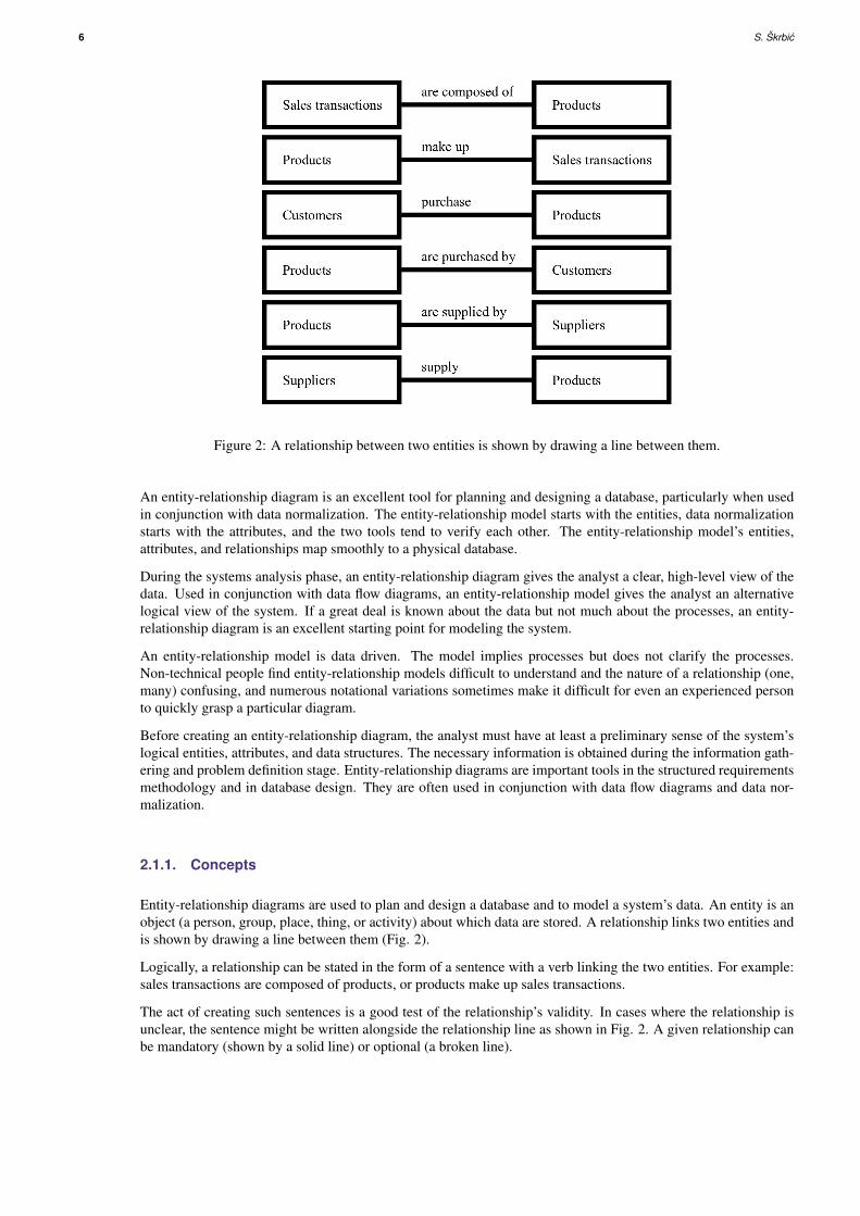
Figure 2: A relationship between two entities is shown by drawing a line between them.

An entity-relationship diagram is an excellent tool for planning and designing a database, particularly when usedin conjunction with data normalization. The entity-relationship model starts with the entities, data normalizationstarts with the attributes, and the two tools tend to verify each other. The entity-relationship model’s entities,attributes, and relationships map smoothly to a physical database.

During the systems analysis phase, an entity-relationship diagram gives the analyst a clear, high-level view of thedata. Used in conjunction with data flow diagrams, an entity-relationship model gives the analyst an alternativelogical view of the system. If a great deal is known about the data but not much about the processes, an entity-relationship diagram is an excellent starting point for modeling the system.

An entity-relationship model is data driven. The model implies processes but does not clarify the processes.Non-technical people find entity-relationship models difficult to understand and the nature of a relationship (one,many) confusing, and numerous notational variations sometimes make it difficult for even an experienced personto quickly grasp a particular diagram.

Before creating an entity-relationship diagram, the analyst must have at least a preliminary sense of the system’slogical entities, attributes, and data structures. The necessary information is obtained during the information gath-ering and problem definition stage. Entity-relationship diagrams are important tools in the structured requirementsmethodology and in database design. They are often used in conjunction with data flow diagrams and data nor-malization.

2.1.1. Concepts

Entity-relationship diagrams are used to plan and design a database and to model a system’s data. An entity is anobject (a person, group, place, thing, or activity) about which data are stored. A relationship links two entities andis shown by drawing a line between them (Fig. 2).

Logically, a relationship can be stated in the form of a sentence with a verb linking the two entities. For example:sales transactions are composed of products, or products make up sales transactions.

The act of creating such sentences is a good test of the relationship’s validity. In cases where the relationship isunclear, the sentence might be written alongside the relationship line as shown in Fig. 2. A given relationship canbe mandatory (shown by a solid line) or optional (a broken line).


Figure 3: One-to-one relationship.

Figure 4: One-to-many relationship.

2.1.2. Relationships

For a variety of reasons, some relationships are more stable and easier to maintain than others. (A detailed discus-sion of the underlying database theory is beyond the scope of this course.) Cardinality, a measure of the relatedentities’ relative number of occurrences, is an important predictor of the strength of the relationship.

In a one-to-one relationship, each occurrence of entity A is associated with one and only one occurrence of entityB, and each occurrence of entity B is associated with one and only one occurrence of entity A (Fig. 3).

For example, imagine that an instructor maintains examination grades for each student in his or her class. Thereare two entities in this example: Students and Exams. For each Student there is one and only one Exam, and foreach Exam there is one and only one Student.

Graphically, a one-to-one relationship is described by drawing short crossing lines at both ends of the line that linksthe two entities (Fig. 3). However, some practitioners simply show the relationship line with no embellishment,and other symbols are used as well.

In a one-to-many relationship, each occurrence of entity A is associated with one or more occurrences of entity B,but each occurrence of entity B is associated with only one occurrence of entity A (Fig. 4).

For example, a student’s grade in most courses is based on numerous grade factors (such as exams, papers, andprojects). A given Student has several different Grade factors, but a given Grade factor is associated with one andonly one Student.

Graphically, a one-to-many relationship is shown by drawing a short crossing line (or no extra marking) at the’one-end’ and a small triangle (sometimes called a crow’s foot) at the ’many-end’ of the relationship line (Fig. 4).Some practitioners use other symbols, however.

In a many-to-many relationship, each occurrence of entity A is associated with one or more occurrences of entityB, and each occurrence of entity B is associated with one or more occurrences of entity A (Fig. 5). For example,a student’s end-of-term Grade report can list several Courses, and a given Course can appear on many students’Grade reports.

Graphically, a many-to-many relationship is shown by drawing a crow’s foot at both ends of the relationship line(Fig. 5). Again, some practitioners use other symbols.

Here we focus on one-to-one, one-to-many, and many-to-many relationships, other types of relationships arepossible. Sometimes entities are mutually exclusive, with A linked to either B or C, but not both. In a mutuallyinclusive relationship, if A is linked to B it must also be linked to C. Zero cardinality implies that an occurrence of

8 S. Skrbic

Figure 5: Many-to-many relationship.

Figure 6: A many-to-many relationship can often be converted to two one-to-many relationships.

A means no occurrence of B. Cross-links and loops can exist, too. A recursive relationship is shown by drawing asemicircle from the entity back to itself.

For a variety of reasons, one-to-many relationships tend to be the most stable. Consequently, a primary objec-tive of entity-relationship modeling is to convert one-to-one and many-to-many relationships into one-to-manyrelationships.

One-to-one relationships can often be merged. Generally, entities that share a one-to-one relationship are really thesame entity and should be merged unless there is a good reason to keep them separate. Note that not all one-to-onerelationships can be merged, however. For example, imagine a relationship between athletes and drug tests. Thereis one Drug test per Athlete and one Athlete per Drug test, so the relationship is clearly one-to-one. In this case,however, because merging the entities would probably violate security requirements (and possibly the law), thereis a good logical reason to maintain separate entities.

Many-to-many relationships can cause maintenance problems. For example, Fig. 6 shows a many-to-many rela-tionship between Inventory and Supplier. Each product in Inventory can have more than one Supplier, and eachSupplier can carry more than one product. If a list of suppliers were stored in Inventory, adding or deleting asupplier might mean updating several Inventory occurrences. Likewise, listing products in Supplier could meanchanging several Supplier occurrences if a single product were added or deleted.

One solution is to create a new entity that has a one-to-many relationship with both original entities. For example,imagine a new entity called Item ordered (Fig. 6). Given such a design, a given product in Inventory can appearon several active Items ordered, but each Item ordered is for one and only one product. Likewise, a given suppliercan appear on several active Items ordered, but each Item ordered lists one and only supplier. Note that a givenItem ordered links a specific product in Inventory with a specific occurrence of Supplier. The many-to-manyrelationship has been converted to two one-to-many relationships.

2.1.3. ER diagrams

Assume a preliminary analysis of a retail sales application suggests four primary entities: customer, sales, inven-tory, and supplier. The Sales, Customer, and Inventory entities are related as follows. Customer initiates Sales.Sales are drawn from Inventory.

The first relationship is one-to-many (Fig. 7); a given Customer can have many Sales transactions, but a given Saleis associated with one and only one Customer. However, the second relationship is many-to-many because a givenSale can include several products from Inventory and a given product in Inventory can appear in many Sales.


Figure 7: Customer, Sales and Inventory.

Figure 8: Resolving the many-to-many relationship calls for a new entity.

To resolve the many-to-many relationship, create a new entity, Item sold, that has a one-to-many relationship withboth Sales and Inventory (Fig. 8). A given Sales transaction can list many Items sold, but a given Item sold isassociated with one and only one Sales transaction. A given product in Inventory can appear in many Items sold,but a given Item sold lists one and only one product. (Think of an Item sold as one line in a list of productspurchased on a sales invoice.)

There is one possible source of confusion about the Inventory entity that might need clarification. A specific 19-inch color television set is an example of a single occurrence of that entity, but Inventory might hold numerousvirtually identical television sets. For inventory control purposes, tracking television sets (a class of occurrences)is probably good enough. However, the Customer purchases a specific television set (identified, perhaps, byconcatenating the serial number to the stock number). Thus a given Item sold lists one and only one occurrence ofInventory.

The relationship between Inventory and Supplier (Fig. 9) is many-to-many because a given product can have manysuppliers and a given supplier can supply many different products. Many-to-many relationships must be resolved,so add a new entity called Item ordered to the model, yielding two one-to-many relationships.

Figure 9: Creating a new entity called item ordered.

10 S. Skrbic

Figure 10: The finished entity-relationship model.

Title Year Length GenreDie Hard: With a Vengeance 1995 131 actionPulp Fiction 1994 154 crimeKing Kong 2005 187 adventure

Table 1: The relation Movies.

Finally, the Inventory entity is related to both Item sold and Item ordered, so combine the two partial diagrams toform a single entity-relationship model (Fig. 10).

2.2. Relational Model

The relational model gives us a single way to represent data: as a two-dimensional table called a relation. Table1 is an example of a relation, which we shall call Movies. The rows each represent a movie, and the columnseach represent a property of movies. We shall introduce the most important terminology regarding relations, andillustrate them with the Movies relation.

2.2.1. Attributes

The columns of a relation are named by attributes. In table 1 the attributes are title, year, length, and genre.Attributes appear at the tops of the columns. Usually, an attribute describes the meaning of entries in the columnbelow. For instance, the column with attribute length holds the length, in minutes, of each movie.


2.2.2. Schemas

The name of a relation and the set of attributes for a relation is called the schema for that relation. We show theschema for the relation with the relation name followed by a parenthesized list of its attributes. Thus, the schemafor relation Movies is

Movies(title, year, length, genre).

We shall generally follow the convention that relation names begin with a capital letter, and attribute names beginwith a lower-case letter. The attributes in a relation schema are a set, not a list. However, in order to talk aboutrelations we often must specify a ”standard” order for the attributes. Thus, whenever we introduce a relationschema with a list of attributes, as above, we shall take this ordering to be the standard order whenever we displaythe relation or any of its rows.

In the relational model, a database consists of one or more relations. The set of schemas for the relations of adatabase is called a relational database schema, or just a database schema.

2.2.3. Tuples

The rows of a relation, other than the header row containing the attribute names, are called tuples. A tuple hasone component for each attribute of the relation. For instance, the first of the three tuples in table 1 has thefour components Die Hard: With a Vengeance, 1995, 131, action for attributes title, year, length, and genre,respectively. When we wish to write a tuple in isolation, not as part of a relation, we normally use commas toseparate components, and we use parentheses to surround the tuple. For example,

(DieHard : With aV engeance, 1995, 131, action)

is the first tuple of table 1. Notice that when a tuple appears in isolation, the attributes do not appear, so someindication of the relation to which the tuple belongs must be given. We shall always use the order in which theattributes were listed in the relation schema.

2.2.4. Domains

The relational model requires that each component of each tuple be atomic; that is, it must be of some elementarytype such as integer or string. It is not permitted for a value to be a record structure, set, list, array, or any othertype that reasonably can have its values broken into smaller components. It is further assumed that associatedwith each attribute of a relation is a domain, that is, a particular elementary type. The components of any tupleof the relation must have, in each component, a value that belongs to the domain of the corresponding column.For example, tuples of the Movies relation of table 1 must have a first component that is a string, second and thirdcomponents that are integers, and a fourth component whose value is a string.

It is possible to include the domain, or data type, for each attribute in a relation schema. We shall do so byappending a colon and a type after attributes. For example, we could represent the schema for the Movies relationas:

Movies(title : string, year : integer, length : integer, genre : string).

2.2.5. Representations of a Relation

Relations are sets of tuples, not lists of tuples. Thus the order in which the tuples of a relation are presented isimmaterial. For example, we can list the three tuples of table 1 in any of their six possible orders, and the relationis ”the same” as in table 1. Moreover, we can reorder the attributes of the relation as we choose, without changing

12 S. Skrbic

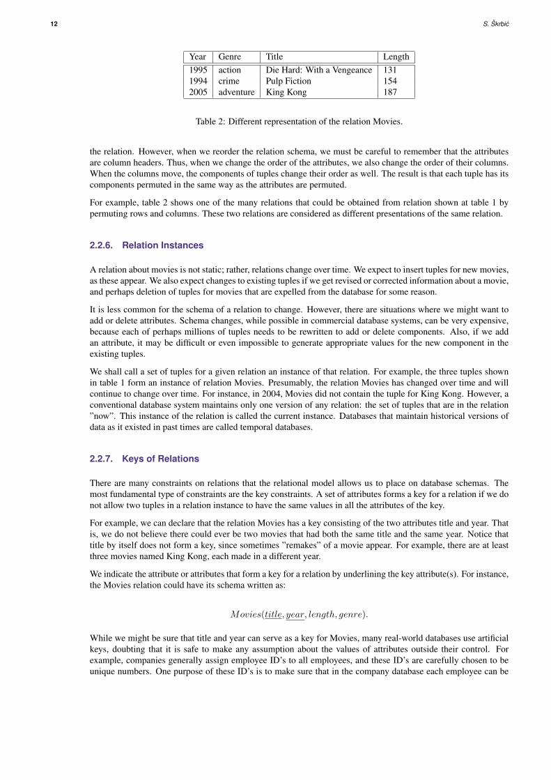
Year Genre Title Length1995 action Die Hard: With a Vengeance 1311994 crime Pulp Fiction 1542005 adventure King Kong 187

Table 2: Different representation of the relation Movies.

the relation. However, when we reorder the relation schema, we must be careful to remember that the attributesare column headers. Thus, when we change the order of the attributes, we also change the order of their columns.When the columns move, the components of tuples change their order as well. The result is that each tuple has itscomponents permuted in the same way as the attributes are permuted.

For example, table 2 shows one of the many relations that could be obtained from relation shown at table 1 bypermuting rows and columns. These two relations are considered as different presentations of the same relation.

2.2.6. Relation Instances

A relation about movies is not static; rather, relations change over time. We expect to insert tuples for new movies,as these appear. We also expect changes to existing tuples if we get revised or corrected information about a movie,and perhaps deletion of tuples for movies that are expelled from the database for some reason.

It is less common for the schema of a relation to change. However, there are situations where we might want toadd or delete attributes. Schema changes, while possible in commercial database systems, can be very expensive,because each of perhaps millions of tuples needs to be rewritten to add or delete components. Also, if we addan attribute, it may be difficult or even impossible to generate appropriate values for the new component in theexisting tuples.

We shall call a set of tuples for a given relation an instance of that relation. For example, the three tuples shownin table 1 form an instance of relation Movies. Presumably, the relation Movies has changed over time and willcontinue to change over time. For instance, in 2004, Movies did not contain the tuple for King Kong. However, aconventional database system maintains only one version of any relation: the set of tuples that are in the relation”now”. This instance of the relation is called the current instance. Databases that maintain historical versions ofdata as it existed in past times are called temporal databases.

2.2.7. Keys of Relations

There are many constraints on relations that the relational model allows us to place on database schemas. Themost fundamental type of constraints are the key constraints. A set of attributes forms a key for a relation if we donot allow two tuples in a relation instance to have the same values in all the attributes of the key.

For example, we can declare that the relation Movies has a key consisting of the two attributes title and year. Thatis, we do not believe there could ever be two movies that had both the same title and the same year. Notice thattitle by itself does not form a key, since sometimes ”remakes” of a movie appear. For example, there are at leastthree movies named King Kong, each made in a different year.

We indicate the attribute or attributes that form a key for a relation by underlining the key attribute(s). For instance,the Movies relation could have its schema written as:

Movies(title, year, length, genre).

While we might be sure that title and year can serve as a key for Movies, many real-world databases use artificialkeys, doubting that it is safe to make any assumption about the values of attributes outside their control. Forexample, companies generally assign employee ID’s to all employees, and these ID’s are carefully chosen to beunique numbers. One purpose of these ID’s is to make sure that in the company database each employee can be


distinguished from all others, even if there are several employees with the same name. Thus, the employee-IDattribute can serve as a key for a relation about employees.

In US corporations, it is normal for every employee to have a Social-Security number. If the database has anattribute that is the Social-Security number, then this attribute can also serve as a key for employees. There isnothing wrong with there being several choices of key, as there would be for employees having both employeeID’s and Social-Security numbers. These keys are then called equivalent keys, and one of them has to be chosenand used. The chosen key is called the primary key of a relation.

2.2.8. Functional Dependencies

First, we need to define the notion of r-value. If we have a set of attributes R = {Ai|i = 1, . . . , k}, an r-value,denoted by t[R] is a function that maps every attribute from R into a value from one record. Essentially, an r-valueis a tuple, but it can also be only a part of a tuple too.

Functional dependency is a type of constraint that generalizes the notion of key constraint. It is defined on the setof relations and allows expression of inter relational constraints.

Expression of type f : X → Y , where X and Y are sets of attributes, is called a functional dependency. It canbe read that X functionally determines Y, and that Y functionally depends on X. I means that every element ofthe domain of the attribute X is mapped to element from domain of Y. Another words, if a value for the set ofattributes X is given, then it uniquely determines a value for the set of attributes Y.

Formally, if a relation r over a set of attributes U is given, and X,Y ⊆ U , then a set of tuples of relation r satisfiesa functional dependency f : X → Y if for every two tuples u and v in r the following holds:

u[X] = v[X] =⇒ u[Y ] = v[Y ].

Functional dependencies are used to express constraints that could not be expressed by key constraints, especiallyinter-relation constraints.

Closure of a set of functional dependencies F , denoted by F+ is a set of all functional dependencies from F andthose that can be derived from F using rules of inference. One set of rules of inference are Armstrong’s axioms[1]. Let us assume that a set of functional dependencies F is defined over a set of attributes U , and that X , Y , Zand W are subsets of U . Then the Armstrong’s axioms are the following

1. Reflexivity: if Y ⊆ X , then X → Y ,

2. Augmentation: if if X → Y and Z ⊆W , then XW → Y Z,

3. Pseudo transitivity: if X → Y and YW → Z, then XW → Z.

Now we can give an alternative definition of a key constraint. A set of attributes X ⊆ R is a key of a relationconsisting of the set of attributes R and a set of functional dependencies F if and only if the following holds:

1. X → Y ⊆ F+,

2. (∀Y ⊂ X)(Y → R /∈ F+).

2.2.9. Referential integrity

The most important inter-relational constraint is a referential integrity. It is used to create links between tables.Informally, for referential integrity to hold, any field in a table that is declared a foreign key can contain onlyvalues from a parent table’s primary key. For instance, deleting a record that contains a value referred to by aforeign key in another table would break referential integrity.

14 S. Skrbic

PId LastName FirstName Address City1 Smith John 5th Avenue 10 New York2 Barnes Kate King’s Avenue 23 London3 Brown Neil Pitt Street 20 London

Table 3: Example database table.

For example, let us expand our movies database model with another table that represents movie directors. We canadd a table that has three attributes - personal ID, first name and last name. Personal ID is a primary key. Nowwe can make a link between table Movies and Directors by adding the attribute personal ID under name directorto the Movies table and demanding that this attribute has only values that already exist in the Directors table. Thistype of constraint is called referential integrity. Attribute director is called a foreign key. Our database could thenbe specified like this:

Movies(title, year, length, genre, director),

Directors(personal ID, first name, last name),

In addition, functional dependency personal ID → director has to hold. Moreover, there is a separate notationfor referential integrity constraint. In this case, we would write:

Movies[director] ⊆ Directors[personal ID].

It should be noted that a foreign key can contain more than one attribute if the primary key that it is drawn fromcontains more than one attribute.

Formal definition is a bit more complex. Let r1 and r2 be two relations containing a set of attributes R1 andR2 respectively. Let A1, . . . , An ∈ R1 and B1, . . . , Bn ∈ R2, and let B1, . . . , Bn be the key of relation r2.Referential integrity r1[A1, . . . , An] ⊆ r2[B1, . . . , Bn] holds if and only if for every tuple t1 from r1 exists a tuplet2 from r2 so that t1[Ak] = t2[Bk] for every k = {1, . . . , n}.

3. SQL

SQL is a standard language for accessing and manipulating databases. SQL stands for Structured Query Language.It lets you access and manipulate databases. Although SQL is an ANSI (American National Standards Institute)standard, there are many different versions of the SQL language. SQL can:

• execute queries against a database,

• retrieve data from a database,

• insert, update and delete records in a database,

• create new databases and tables. . .

Below is an example of a table called ”Persons”. The table contains three records (one for each person) and fivecolumns: PId, LastName, FirstName, Address and City.

Most of the actions we need to perform on a database are done with SQL statements. The following SQL statementwill select all the records in the ”Persons” table:

SELECT ∗ FROM P e r s o n s


LastName FirstNameSmith JohnBarnes KateBrown Neil

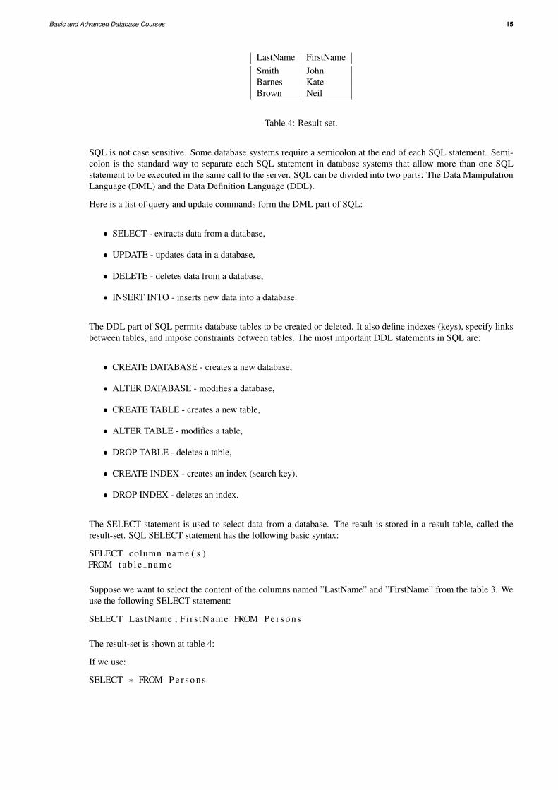
Table 4: Result-set.

SQL is not case sensitive. Some database systems require a semicolon at the end of each SQL statement. Semi-colon is the standard way to separate each SQL statement in database systems that allow more than one SQLstatement to be executed in the same call to the server. SQL can be divided into two parts: The Data ManipulationLanguage (DML) and the Data Definition Language (DDL).

Here is a list of query and update commands form the DML part of SQL:

• SELECT - extracts data from a database,

• UPDATE - updates data in a database,

• DELETE - deletes data from a database,

• INSERT INTO - inserts new data into a database.

The DDL part of SQL permits database tables to be created or deleted. It also define indexes (keys), specify linksbetween tables, and impose constraints between tables. The most important DDL statements in SQL are:

• CREATE DATABASE - creates a new database,

• ALTER DATABASE - modifies a database,

• CREATE TABLE - creates a new table,

• ALTER TABLE - modifies a table,

• DROP TABLE - deletes a table,

• CREATE INDEX - creates an index (search key),

• DROP INDEX - deletes an index.

The SELECT statement is used to select data from a database. The result is stored in a result table, called theresult-set. SQL SELECT statement has the following basic syntax:

SELECT column name ( s )FROM t a b l e n a m e

Suppose we want to select the content of the columns named ”LastName” and ”FirstName” from the table 3. Weuse the following SELECT statement:

SELECT LastName , F i r s tName FROM P e r s o n s

The result-set is shown at table 4:

If we use:

SELECT ∗ FROM P e r s o n s

16 S. Skrbic

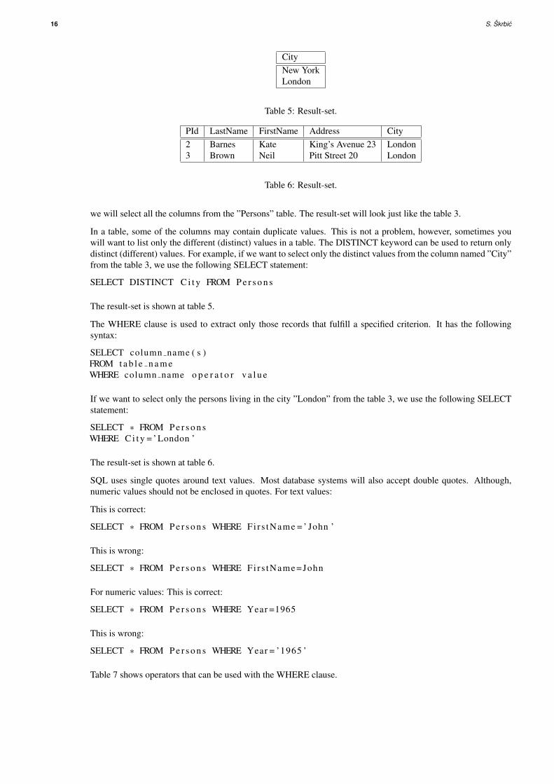
CityNew YorkLondon


PId LastName FirstName Address City2 Barnes Kate King’s Avenue 23 London3 Brown Neil Pitt Street 20 London


we will select all the columns from the ”Persons” table. The result-set will look just like the table 3.

In a table, some of the columns may contain duplicate values. This is not a problem, however, sometimes youwill want to list only the different (distinct) values in a table. The DISTINCT keyword can be used to return onlydistinct (different) values. For example, if we want to select only the distinct values from the column named ”City”from the table 3, we use the following SELECT statement:

SELECT DISTINCT C i t y FROM P e r s o n s

The result-set is shown at table 5.

The WHERE clause is used to extract only those records that fulfill a specified criterion. It has the followingsyntax:

SELECT column name ( s )FROM t a b l e n a m eWHERE column name o p e r a t o r v a l u e

If we want to select only the persons living in the city ”London” from the table 3, we use the following SELECTstatement:

SELECT ∗ FROM P e r s o n sWHERE C i t y = ’ London ’


SQL uses single quotes around text values. Most database systems will also accept double quotes. Although,numeric values should not be enclosed in quotes. For text values:

This is correct:

SELECT ∗ FROM P e r s o n s WHERE Fi r s tName = ’ John ’

This is wrong:

SELECT ∗ FROM P e r s o n s WHERE Fi r s tName =John

For numeric values: This is correct:

SELECT ∗ FROM P e r s o n s WHERE Year =1965

This is wrong:

SELECT ∗ FROM P e r s o n s WHERE Year = ’1965 ’

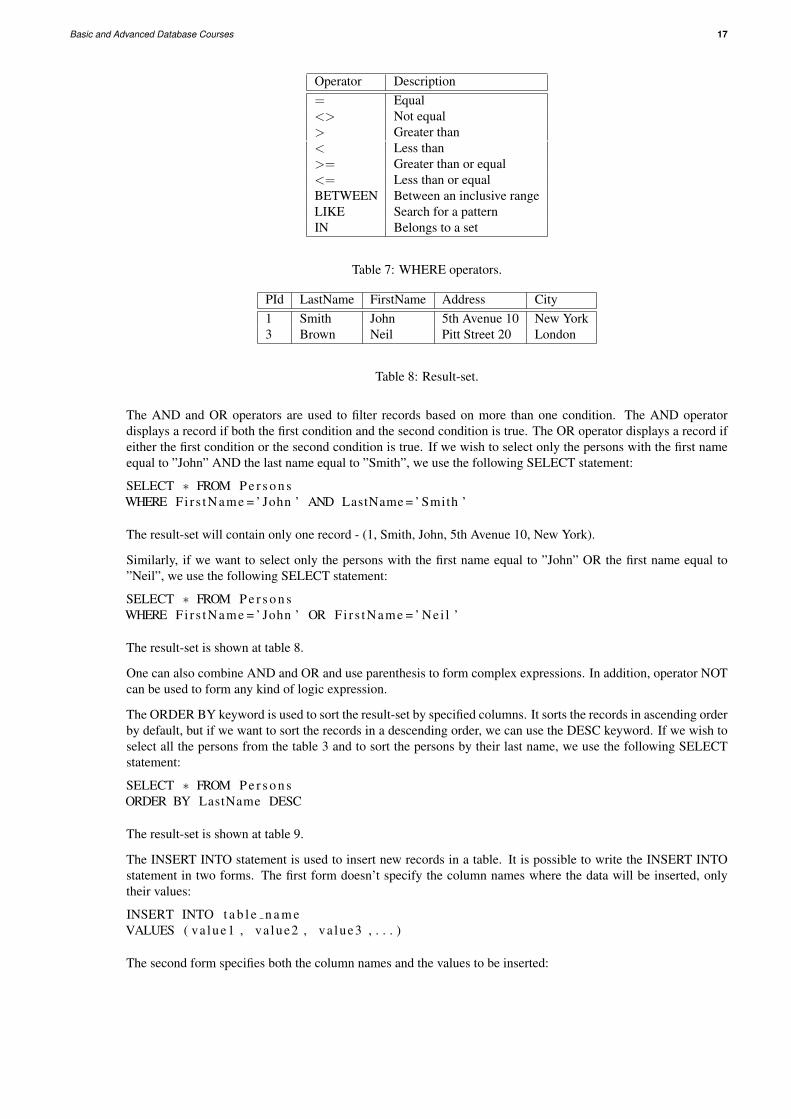
Table 7 shows operators that can be used with the WHERE clause.


Operator Description= Equal<> Not equal> Greater than< Less than>= Greater than or equal<= Less than or equalBETWEEN Between an inclusive rangeLIKE Search for a patternIN Belongs to a set

Table 7: WHERE operators.

PId LastName FirstName Address City1 Smith John 5th Avenue 10 New York3 Brown Neil Pitt Street 20 London


The AND and OR operators are used to filter records based on more than one condition. The AND operatordisplays a record if both the first condition and the second condition is true. The OR operator displays a record ifeither the first condition or the second condition is true. If we wish to select only the persons with the first nameequal to ”John” AND the last name equal to ”Smith”, we use the following SELECT statement:

SELECT ∗ FROM P e r s o n sWHERE Fi r s tName = ’ John ’ AND LastName = ’ Smith ’

The result-set will contain only one record - (1, Smith, John, 5th Avenue 10, New York).

Similarly, if we want to select only the persons with the first name equal to ”John” OR the first name equal to”Neil”, we use the following SELECT statement:

SELECT ∗ FROM P e r s o n sWHERE Fi r s tName = ’ John ’ OR Fi r s tName = ’ Nei l ’


One can also combine AND and OR and use parenthesis to form complex expressions. In addition, operator NOTcan be used to form any kind of logic expression.

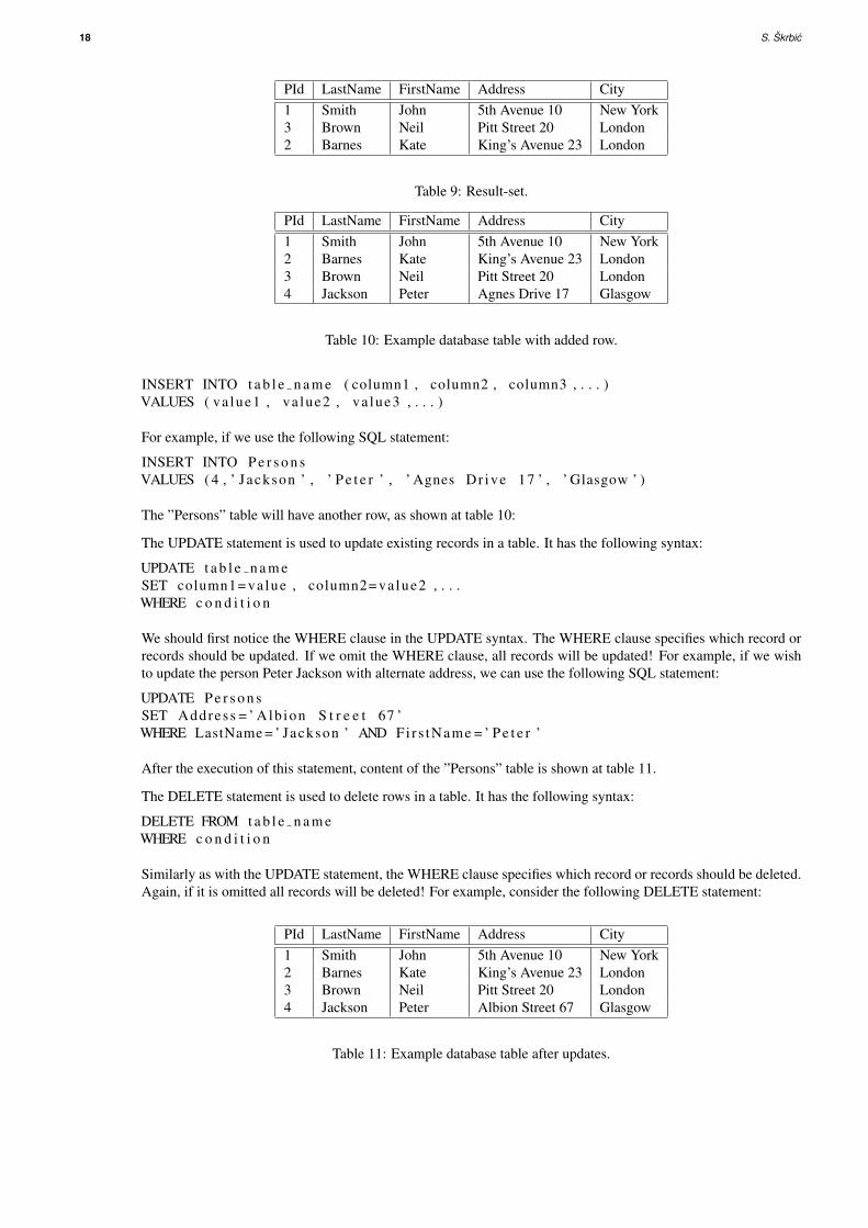
The ORDER BY keyword is used to sort the result-set by specified columns. It sorts the records in ascending orderby default, but if we want to sort the records in a descending order, we can use the DESC keyword. If we wish toselect all the persons from the table 3 and to sort the persons by their last name, we use the following SELECTstatement:

SELECT ∗ FROM P e r s o n sORDER BY LastName DESC


The INSERT INTO statement is used to insert new records in a table. It is possible to write the INSERT INTOstatement in two forms. The first form doesn’t specify the column names where the data will be inserted, onlytheir values:

INSERT INTO t a b l e n a m eVALUES ( va lue1 , va lue2 , va lue3 , . . . )

The second form specifies both the column names and the values to be inserted:

18 S. Skrbic

PId LastName FirstName Address City1 Smith John 5th Avenue 10 New York3 Brown Neil Pitt Street 20 London2 Barnes Kate King’s Avenue 23 London


PId LastName FirstName Address City1 Smith John 5th Avenue 10 New York2 Barnes Kate King’s Avenue 23 London3 Brown Neil Pitt Street 20 London4 Jackson Peter Agnes Drive 17 Glasgow

Table 10: Example database table with added row.

INSERT INTO t a b l e n a m e ( column1 , column2 , column3 , . . . )VALUES ( va lue1 , va lue2 , va lue3 , . . . )

For example, if we use the following SQL statement:

INSERT INTO P e r s o n sVALUES ( 4 , ’ Jackson ’ , ’ P e t e r ’ , ’ Agnes Dr ive 17 ’ , ’ Glasgow ’ )

The ”Persons” table will have another row, as shown at table 10:

The UPDATE statement is used to update existing records in a table. It has the following syntax:

UPDATE t a b l e n a m eSET column1= va lue , column2= va lue2 , . . .WHERE c o n d i t i o n

We should first notice the WHERE clause in the UPDATE syntax. The WHERE clause specifies which record orrecords should be updated. If we omit the WHERE clause, all records will be updated! For example, if we wishto update the person Peter Jackson with alternate address, we can use the following SQL statement:

UPDATE P e r s o n sSET Address = ’ Alb ion S t r e e t 67 ’WHERE LastName = ’ Jackson ’ AND Fi r s tName = ’ P e t e r ’

After the execution of this statement, content of the ”Persons” table is shown at table 11.

The DELETE statement is used to delete rows in a table. It has the following syntax:

DELETE FROM t a b l e n a m eWHERE c o n d i t i o n

Similarly as with the UPDATE statement, the WHERE clause specifies which record or records should be deleted.Again, if it is omitted all records will be deleted! For example, consider the following DELETE statement:

PId LastName FirstName Address City1 Smith John 5th Avenue 10 New York2 Barnes Kate King’s Avenue 23 London3 Brown Neil Pitt Street 20 London4 Jackson Peter Albion Street 67 Glasgow

Table 11: Example database table after updates.


DELETE FROM P e r s o n sWHERE LastName = ’ Jackson ’ AND Fi r s tName = ’ P e t e r ’

Clearly, after the execution, the fourth record will be deleted. So, the content of the “Persons” table will be thesame as it was at the start, shown at table 3.

4. Normalization

Normalization is a design technique that is widely used as a guide in designing relational databases. It is essentiallya two step process that puts data into tabular form by removing repeating groups and then removes duplicates fromrelational tables.

Normalization theory is based on the concepts of normal forms. A database is said to be in a particular normalform if it satisfied a certain set of constraints. There are currently at least eight normal forms that have beendefined. In this section, we will cover the first three normal forms that were defined by the creator of the relationalmodel, E. F. Codd [4]. Codd and Raymond Boyce defined the Boyce-Codd Normal Form (BCNF) in 1974 [5].Higher normal forms like fourth [8], fifth [9] and domain/key normal form [10] were defined by other theorists insubsequent years. The most recent is the Sixth normal form (6NF) introduced by Chris Date, Hugh Darwen, andNikos Lorentzos in 2002 [6].

4.1. Basic Concepts

The goal of normalization is to create a set of relational tables that are free of redundant data and that can beconsistently and correctly modified. This means that all tables in a relational database should be in the thirdnormal form (3NF). A relational table is in 3NF if and only if all non-key columns are:

1. mutually independent and

2. fully dependent on the primary key.

Mutual independence means that no non-key column is dependent upon any combination of the other columns.The first two normal forms are intermediate steps to achieve the goal of having all tables in 3NF. In order to betterunderstand the 2NF and higher forms, it is necessary to understand the concepts of functional dependencies andlossless decomposition.

The concept of functional dependencies is the basis for the first three normal forms. As explained earlier, a column,Y, of the relational table R is said to be functionally dependent upon column X of R if and only if each value of Xin R is associated with precisely one value of Y at any given time. X and Y may be composite. Saying that columnY is functionally dependent upon X is the same as saying the values of column X identify the values of column Y.If column X is a primary key, then all columns in the relational table R must be functionally dependent upon X.

Full functional dependence applies to tables with composite keys. Column Y in relational table R is fully functionalon X of R if it is functionally dependent on X and not functionally dependent upon any subset of X. Full functionaldependence means that when a primary key is composite, made of two or more columns, then the other columnsmust be identified by the entire key and not just some of the columns that make up the key.

Simply stated, normalization is the process of removing redundant data from relational tables by decomposing(splitting) a relational table into smaller tables by projection. The goal is to have only primary keys on the lefthand side of a functional dependency. In order to be correct, decomposition must be lossless. That is, the newtables can be recombined by a natural join to recreate the original table without creating any spurious or redundantdata.

Here is some sample data used to illustrate the process of normalization. A company obtains parts from a numberof suppliers. Each supplier is located in one city. A city can have more than one supplier located there and each

20 S. Skrbic

s# status city p# qtys1 20 London p1 300s1 20 London p2 200s1 20 London p3 400s1 20 London p4 200s1 20 London p5 100s1 20 London p6 100s2 10 Paris p1 300s2 10 Paris p2 400s3 10 Paris p2 200s4 20 London p2 200s4 20 London p4 300s4 20 London p5 400

Table 12: Table in 1NF.

city has a status code associated with it. Each supplier may provide many parts. The company creates a simplerelational table to store this information that can be expressed in relational notation as:

FIRST (s#, status, city, p#, qty),

where:

• s# is a supplier identifcation number,

• status is a status code assigned to city,

• city is a name of city where supplier is located,

• p# is a part number of part supplied and

• qty is a quantity of parts supplied to date.

In order to uniquely associate quantity supplied (qty) with part (p#) and supplier (s#), a composite primary keycomposed of s# and p# is used.

4.2. First Normal Form

A relational table, by definition, is in first normal form. All values of the columns are atomic. That is, they containno repeating values. Table 12 shows the table FIRST in 1NF.

Although the table FIRST is in 1NF it contains redundant data. For example, information about the supplier’slocation and the location’s status have to be repeated for every part supplied. Redundancy causes what are calledupdate anomalies. Update anomalies are problems that arise when information is inserted, deleted, or updated.For example, the following anomalies could occur in FIRST:

1. INSERT. The fact that a certain supplier (s5) is located in a particular city (Athens) cannot be added untilthey supplied a part.

2. DELETE. If a row is deleted, then not only is the information about quantity and part lost but also informa-tion about the supplier.

3. UPDATE. If supplier s1 moved from London to New York, then six rows would have to be updated withthis new information.


s# status citys1 20 Londons2 10 Pariss3 10 Pariss4 20 Londons5 30 Athens

Table 13: SUPPLIER table.

4.3. Second Normal Form

The definition of second normal form states that only tables with composite primary keys can be in 1NF but not in2NF.

A relational table is in second normal form 2NF if it is in 1NF and every non-key column is fully dependent uponthe primary key. That is, every non-key column must be dependent upon the entire primary key. FIRST is in 1NFbut not in 2NF because status and city are functionally dependent only on the column s# of the composite key (s#,p#). This can be illustrated by listing the functional dependencies in the table:

s#→ (city, status),

city → status,

(s#, p#)→ qty.

If we wanted to transform the table FIRST from 1NF to 2NF we could:

1. Identify any determinants other than the composite key, and the columns they determine.

2. Create and name a new table for each determinant and the unique columns it determines.

3. Move the determined columns from the original table to the new table.

4. The determinate becomes the primary key of the new table.

5. Delete the columns we just moved from the original table except for the determinate which will serve as aforeign key.

The original table may be renamed to maintain semantic meaning. To transform FIRST into 2NF we move thecolumns s#, status, and city to a new table called SUPPLIER. The column s# becomes the primary key of this newtable. The results are shown at tables 13 and 14.

Tables in 2NF but not in 3NF still contain modification anomalies. In the example of SUPPLIER, they are:

1. INSERT. The fact that a particular city has a certain status (Rome has a status of 50) cannot be inserted untilthere is a supplier in the city.

2. DELETE. Deleting any row in SUPPLIER destroys the status information about the city as well as theassociation between supplier and city.

4.4. Third Normal Form

The third normal form requires that all columns in a database are dependent only upon the primary key. A moreformal definition is:

22 S. Skrbic

s# p# qtys1 p1 300s1 p2 200s1 p3 400s1 p4 200s1 p5 100s1 p6 100s2 p1 300s2 p2 400s3 p2 200s4 p2 200s4 p4 300s4 p5 400

Table 14: PARTS table.

A database is in the third normal form (3NF) if it is already in 2NF and every non-key column is non transitivelydependent upon its primary key. In other words, all non-key attributes are functionally dependent only upon theprimary key.

Table PARTS is already in 3NF. The non-key column, qty, is fully dependent upon the primary key (s#, p#).SUPPLIER is in 2NF but not in 3NF because it contains a transitive dependency. A transitive dependency occurswhen a non-key column that is a determinant of the primary key is the determinate of other columns. The conceptof a transitive dependency can be illustrated by showing the functional dependencies in SUPPLIER:

SUPPLIER.s#→ SUPPLIER.status,

SUPPLIER.s#→ SUPPLIER.city,

SUPPLIER.city → SUPPLIER.status.

Note that SUPPLIER.status is determined both by the primary key s# and the non-key column city. The processof transforming a table into 3NF is the following:

1. Identify any determinants, other than primary key, and the columns they determine.

2. Create and name a new table for each determinant and the unique columns it determines.

3. Move the determined columns from the original table to the new table.

4. The determinate becomes the primary key of the new table.

5. Delete the columns you just moved from the original table except for the determinate which will serve as aforeign key.

The original table may be renamed to maintain semantic meaning.

To transform SUPPLIER into 3NF, we create a new table called CITY STATUS and move the columns city andstatus into it. Status is deleted from the original table, city is left behind to serve as a foreign key to CITY STATUS,and the original table is renamed to SUPPLIER CITY to reflect its semantic meaning. The results of putting theoriginal table into 3NF has created three tables. These can be represented as:

PARTS(s#, p#, qty)

SUPPLIER CITY (s#, city)

CITY STATUS(city, status)

PARTS[s#] ⊆ SUPPLIER CITY [s#]

SUPPLIER CITY [s#] ⊆ CITY STATUS[city].


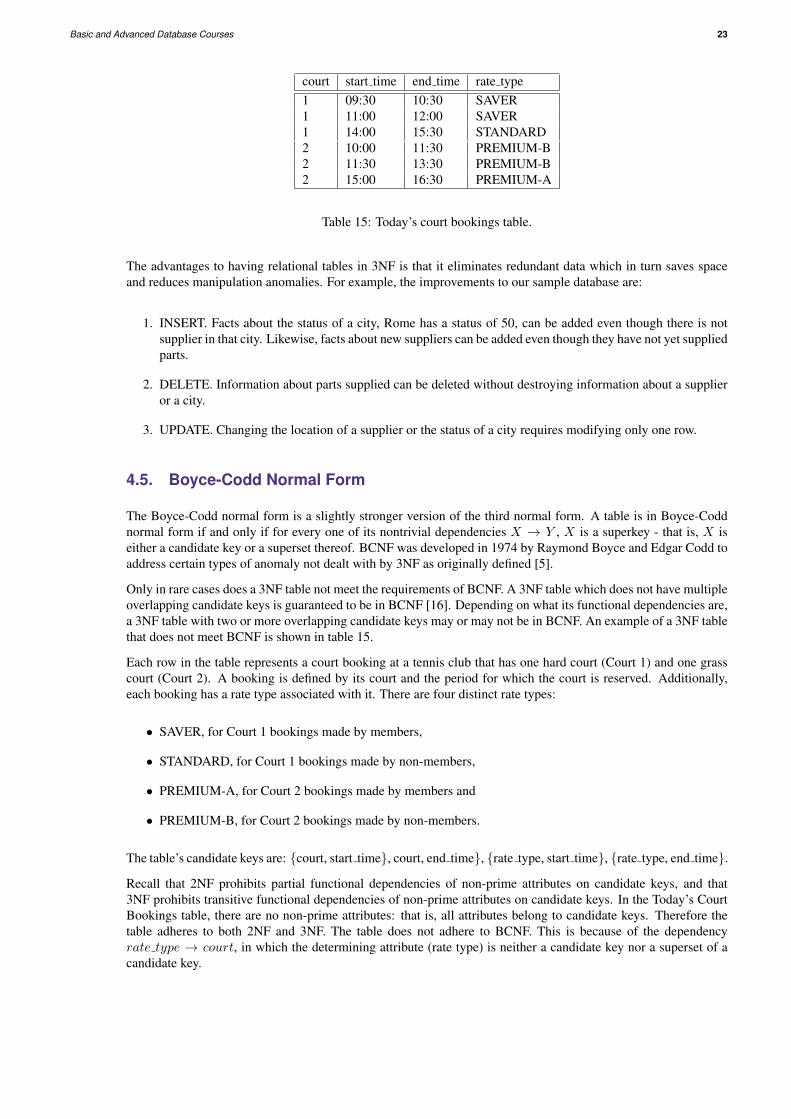
court start time end time rate type1 09:30 10:30 SAVER1 11:00 12:00 SAVER1 14:00 15:30 STANDARD2 10:00 11:30 PREMIUM-B2 11:30 13:30 PREMIUM-B2 15:00 16:30 PREMIUM-A

Table 15: Today’s court bookings table.

The advantages to having relational tables in 3NF is that it eliminates redundant data which in turn saves spaceand reduces manipulation anomalies. For example, the improvements to our sample database are:

1. INSERT. Facts about the status of a city, Rome has a status of 50, can be added even though there is notsupplier in that city. Likewise, facts about new suppliers can be added even though they have not yet suppliedparts.

2. DELETE. Information about parts supplied can be deleted without destroying information about a supplieror a city.

3. UPDATE. Changing the location of a supplier or the status of a city requires modifying only one row.

4.5. Boyce-Codd Normal Form

The Boyce-Codd normal form is a slightly stronger version of the third normal form. A table is in Boyce-Coddnormal form if and only if for every one of its nontrivial dependencies X → Y , X is a superkey - that is, X iseither a candidate key or a superset thereof. BCNF was developed in 1974 by Raymond Boyce and Edgar Codd toaddress certain types of anomaly not dealt with by 3NF as originally defined [5].

Only in rare cases does a 3NF table not meet the requirements of BCNF. A 3NF table which does not have multipleoverlapping candidate keys is guaranteed to be in BCNF [16]. Depending on what its functional dependencies are,a 3NF table with two or more overlapping candidate keys may or may not be in BCNF. An example of a 3NF tablethat does not meet BCNF is shown in table 15.

Each row in the table represents a court booking at a tennis club that has one hard court (Court 1) and one grasscourt (Court 2). A booking is defined by its court and the period for which the court is reserved. Additionally,each booking has a rate type associated with it. There are four distinct rate types:

• SAVER, for Court 1 bookings made by members,

• STANDARD, for Court 1 bookings made by non-members,

• PREMIUM-A, for Court 2 bookings made by members and

• PREMIUM-B, for Court 2 bookings made by non-members.

The table’s candidate keys are: {court, start time}, court, end time}, {rate type, start time}, {rate type, end time}.

Recall that 2NF prohibits partial functional dependencies of non-prime attributes on candidate keys, and that3NF prohibits transitive functional dependencies of non-prime attributes on candidate keys. In the Today’s CourtBookings table, there are no non-prime attributes: that is, all attributes belong to candidate keys. Therefore thetable adheres to both 2NF and 3NF. The table does not adhere to BCNF. This is because of the dependencyrate type → court, in which the determining attribute (rate type) is neither a candidate key nor a superset of acandidate key.

24 S. Skrbic

4.6. Normalization algorithms

There are two basic methods for normalization - decomposition and synthesis. There are many variations to thesemethods, but the ideas are the same. Decomposition method is based on progressive decomposition of databaseschema consisting of all attributes in a database in accordance to constraint given by functional dependencies.Decomposition progresses until a database in desired normal form is obtained. The best normal form that isguaranteed by the algorithm is the Boyce-Codd normal form.

The synthesis method, on the other hand, is based on a completely different approach. It is realized by usingfunctional dependencies only. The input is again, a set of all attributes of a database, together with a set of func-tional dependencies. The output is a database at least in third normal form. Tables are synthesized from functionaldependencies. The basic idea is based on reduction and elimination of redundant functional dependencies fromthe initial set.

Detailed description of these algorithms is way beyond the scope of this text. That information can be found in,for instance [13, 2]. It is important to note that the decomposition method guarantees better normal form thanthe synthesis method. It guarantees that the resulting database will be in the Boyce-Codd normal form, whilethe synthesis algorithm takes us only to the third normal form, in the worst case. This is an advantage of thedecomposition method. On the other hand, the decomposition method does not guarantee the conservation ofinitial set of functional dependencies. It is possible that some nontrivial functional dependencies are lost in theprocess. Important data about the database structure can be lost with them. On the other hand, the synthesismethod guarantees the conservation of the initial set of functional dependencies. There is another importantadvantage of the synthesis method. Its complexity is polynomial, while the complexity of the decompositionmethod is exponential. This gives the synthesis method decisive advantage in the case of large databases.

The fact that the method of synthesis does not necessarily gives a database in BCNF has small significance forpractical usage. In practice, databases in 3NF and not in BCNF are rare. On the other hand, conservation of initialset of functional dependencies is important because it guarantees that the resulting database content will be inaccordance to constraints in the real world expressed by functional dependencies.

Normalization is an important step in database design methodology. However, manual use of normalization al-gorithms can be conducted only with small and simple databases. Automatization of these methods is the onlysolution. Since the method of synthesis has polynomial complexity, in difference to exponential complexity of themethod of decomposition, it is generally a better choice.

References

[1] William Ward Armstrong. Dependency structures of data base relationships. In IFIP Congress, pages580–583, 1974.

[2] Philip A. Bernstein. Synthesizing third normal form relations from functional dependencies. ACMTrans. Database Syst., 1:277–298, December 1976.

[3] Edgar Frank Codd. A relational model of data for large shared data banks. Communications of theACM, 13(6):377–387, 1970.

[4] Edgar Frank Codd. Further normalization of the data base relational model. IBM Research Report, SanJose, California, RJ909, 1971.

[5] Edgar Frank Codd. Recent investigations into relational data base systems. Technical Report RJ1385,IBM, 4 1974.

[6] Chris Date, Hugh Darwen, and Nikos Lorentzos. Temporal Data and the Relational Model. MorganKaufmann Publishers Inc., San Francisco, CA, USA, 2002.

[7] Christopher J. Date. An Introduction to Database Systems, Eighth Edition. Addison Wesley, July 2003.


[8] Ronald Fagin. Multivalued dependencies and a new normal form for relational databases. ACM Trans.Database Syst., 2:262–278, September 1977.

[9] Ronald Fagin. Normal forms and relational database operators. In Proceedings of the 1979 ACMSIGMOD international conference on Management of data, SIGMOD ’79, pages 153–160, New York,NY, USA, 1979. ACM.

[10] Ronald Fagin. A normal form for relational databases that is based on domains and keys. ACM Trans.Database Syst., 6:387–415, September 1981.

[11] Hector Garcia-Molina, Jeffrey D. Ullman, and Jennifer Widom. Database Systems: The Complete Book.Prentice Hall Press, Upper Saddle River, NJ, USA, 2 edition, 2008.

[12] Milos Rackovic, Srdjan Skrbic, and Jovana Vidakovic. Introduction to Databases. Faculty of Science,Novi Sad, Serbia, 2007.

[13] K. V. S. V. N. Raju and Arun K. Majumdar. Fuzzy functional dependencies and lossless join decompo-sition of fuzzy relational database systems. ACM Trans. Database Syst., 13:129–166, June 1988.

[14] Peter Pin shan Chen. The entity-relationship model: Toward a unified view of data. ACM Transactionson Database Systems, 1:9–36, 1976.

[15] A. Silberschatz, H. Korth, and S. Sudarshan. Database Systems Concepts. McGraw-Hill, Inc., NewYork, NY, USA, 5 edition, 2006.

[16] Millist Vincent and Bala Srinivasan. A note on relation schemes which are in 3nf but not in bcnf. Inf.Process. Lett., 48:281–283, December 1993.

Basic and Advanced Database Courses - u-szeged.hu · Basic and Advanced Database ... some basic...

Documents

Transcript of Basic and Advanced Database Courses - u-szeged.hu · Basic and Advanced Database ... some basic...