Forthcoming inJournal of Banking and Finance

Basel III Leverage Ratio Requirement and the Probability of Bank Runs

Jean DermineINSEAD

1 Ayer Rajah AvenueSingapore 138676

jean.dermine@insead.edu

16 December 2014

JEL Classification: G21, G28Keywords: Bank regulation, Basel capital, leverage ratio, credit risk

The author acknowledges the comments of the referees, G. De Nicolo, D. Gromb, M. Massa,J. Peress, and A. Tarazi.

Basel III Leverage Ratio Requirement and the Probability of Bank Runs

Jean DermineINSEAD, Singapore

December 2014

Abstract

A new argument for the Basel III leverage ratio requirement is proposed: the need to limit therisk of a bank run when there is imperfect information on the value of a bank’s assets. In additionto screening and monitoring borrowers, banks provide liquidity insurance with the supply ofshort-term deposits withdrawable on demand. The maturity mismatch creates the risk of adisorderly bank run which can be exacerbated by imperfect information about the value of bankassets. It is shown in a stylized Basel III framework that capital regulation should incorporatea liquidity risk component. Credit risk diversification and/or a reduced probability of loan default which lead to a reduction of Basel III regulatory capital will increase the probability of a bankrun. The leverage ratio rule puts a floor on the Basel III risk-weighed capital ratio, allowing thelimitation of such a risk.

The bank capital regulation set by the Basel Committee on Banking Supervision has attempted

to measure the riskiness of a bank’s on- and off-balance sheet exposure and to fix the amount of

capital needed to limit the probability of default to a desired level of confidence. In 2014, the

Basel Committee announced the introduction of a complementary leverage ratio which is not

anymore risk-weighted. This paper provides an argument for its raison d’etre: the need to limit

the probability of a bank run when there is imperfect information on the value of bank assets.

Under the 1988-Basel I bank capital regulation, the capital required to fund a loan portfolio is a

minimum 8% of assets, whatever the riskiness of bank loans or the degree of credit risk

diversification. The Basel II risk-based capital regulation, adopted in June 2004, applies a

formula that captures better credit risk (Basel Committee, 2004). The framework includes three

pillars: capital regulation, bank supervisors’ oversight and information disclosure. Pillar 1

capital regulation requires bank capital to cover annual credit losses with a 99.9% confidence

level. The degree of credit risk diversification is assessed under Pillar 2 by bank supervisors who

can adjust the capital adequacy requirement. Although the Basel II capital regulation also covers

market and operational risks, the focus of this paper is on credit risk, the main source of bank

failures around the world. The essence of Basel II internal-rating based (IRB) approach was

retained in the revised Basel III capital regulation. The asset risk-weighting is based on the Basel

II framework and higher capital ratios with a much larger emphasis on common equity Tier 1 are

imposed to create a more resilient banking system (Basel Committee, 2010).

Besides credit risk, a second source of risk was prevalent during the global financial crisis:

liquidity risk. Constraints on liquid assets and maturity mismatch are imposed in the Basel III

rules. A liquidity coverage ratio (LCR) ensures that a portfolio of contingent liquid assets can

fund a cash outflow lasting 30 days in a stress scenario (Basel Committee, 2013). And

consultations about a net stable funding ratio are taking place. Its objective is to ensure that

permanent assets are funded with stable funds (Basel Committee, 2014a).

The Pillar 1 risk-weighted Basel II/III capital ratio has been criticized for several reasons:

insufficient capital in a recession, complexity, open to gaming, lack of robustness, and fear of

excess leverage in the economy. Opponents recommend the application of a complementary

simple leverage ratio, equity divided by unweighted balance sheet assets. Preparation for a

mandatory leverage ratio is taking place (Basel Committee, 2014b). Public disclosure on the

leverage ratio will start on January 1 2015. Calibration of the ratio will follow with the objective

of migrating the leverage ratio into a mandatory Pillar 1 capital requirement by January 1 2018.

2

In this paper, we focus on the Pillar 1 risk-weighted capital regulation and the unweighted

leverage ratio, providing an additional argument for its raison d’etre: the need to limit the risk

of a bank run when there is imperfect information about the value of bank assets. We show that

diversification of credit risk or a reduced probability of loan default, which under Basel III

internal ratings-based approach is accompanied by a capital relief, will increase the probability

of a bank run. The effect is caused by imperfect information on loan losses and the shape of the

aggregate loan loss probability distribution. It is shown that the reduction of Pillar 1 Basel III

capital moves the ‘bank run locus’, the set of loan losses which can trigger a bank run, to a higher

probability zone. A unweighted leverage ratio regulation, a floor on the equity-to-asset ratio,

limits the risk of a bank run.

In essence, Basel II models a bank as if one-year maturity assets are funded with one-year

maturity debt. Capital requirement is set to reduce to a desired confidence level the risk of bank

default over a one-year horizon. The one-year horizon was chosen partly because the Basel

Committee wanted to follow market practice in measuring credit risk, but also to reflect banks’

inability to raise equity on a continuous basis. The implicit assumption of perfect matching of

maturities and orderly repayment of deposits at maturity does not recognize that banks offer a

second type of service. In addition to screening and monitoring borrowers, banks provide

liquidity insurance (Diamond and Dybvig, 1983), and long-term assets are funded partly with

short-term deposits that are withdrawable on demand. The maturity mismatch creates a second

type of risk, a bank run by uninsured depositors. Recent examples of bank runs include the

investment banks Bear Stearns and Lehman Brothers during the subprime crisis or the American

money market funds stopping the U.S. Dollar funding of French banks during the euro crisis in

2011. Run by smaller insured retail depositors have also taken place in specific circumstances

of incomplete insurance coverage, delay/hassle in insurance payment, or when the solvency of

the country providing deposit insurance was in doubt. Cases include Northern Rock1 in the

United Kingdom in fall 2007 and banks in Cyprus in March 2013 and Bulgaria in July 2014.

Ideally, bank regulations should be based on models that incorporate both sources of risk: credit

and liquidity risks.

The Basel III liquidity coverage ratio and the net stable funding ratio are not modeled in the

1In the case of the bank run on the British Northern Rock in September 2007,depositors had a 100% coverage for the first £ 2,000, and a 90% coverage for the next £33,000 with a payout time estimated at 6 months.

3

paper. It will be argued that these regulations do not alter the conclusion of the paper regarding

the need for a floor on leverage unless maturity mismatch, an essential function of banks, is

banned. “One of the most important roles performed by banks is the creation of liquid claims on

illiquid assets“ (Goldstein and Pauzner, 2005).

In general discussion on financial stability by central bankers, it is assumed implicitly that the

Basel capital regulation that measures risk with a 99.9% confidence level also contributes to

reducing the risk of bank runs. “Regulators must not start piling new ratios on the existing ones,

adding further requirements (leverage ratios, special ratios on large systematically important

institutions, anti-cyclical capital buffers) to the normal - and revamped- Basel 2 risk-based

system” (de Larosière, 2009). But not everybody agrees that the higher risk-weighted capital

ratio of Basel III provides all the answers. Sheila Bair, former Chairman of the FDIC, justifies

the need for an effective floor on leverage by the concern that risk-weighted capital designed in

periods of prosperity could lead to insufficient capital when the credit cycle deteriorates.2

Haldane (2012) argues that it is too complex and open to gaming with an ‘optimization of risk-

weighted assets’. He proposes a simple and transparent leverage ratio, equity over unweighted

assets. Jarrow (2012) argues that the leverage ratio is more robust to estimation errors. Another

concern was the build-up of leverage in the economy. This led the Financial Stability Forum

(2009, p.15) to also recommend a simple, non-risk based measure to complement the risk-based

approach of Basel II. These five concerns with the risk-weighted capital ratios - insufficient

capital in a recession, complexity, open to gaming, lack of robustness and fear of excess leverage

in the economy - led to the revised Basel III capital regulation and the introduction of a

complementary leverage ratio (Basel Committee, 2010 and 2014b).3 An additional argument is

presented in this paper: the need to limit the risk of a disorderly bank run, risk which is amplified

by imperfect information on the value of bank assets.

Finally, the paper provides a new rationale for the empirical observations that bank capital often

exceeds the Basel regulatory level (Flannery and Rangan, 2002). This rationale is complementary

2In “A Special Report on International Banking”, The Economist, 19 May 2007. TheFDIC imposes a second capital ratio, the leverage ratio, defined as the ratio of Tier 1 overunweighted balance sheet assets.

3In December 2008, Switzerland imposed a leverage ratio on its two largest banks,Credit Suisse and UBS. On July 2, 2013, the US Federal Reserve Board approved the BaselIII rules which include a leverage ratio. The EU will require banks to publish their individualleverage ratios from 2015 and decide by 2018 whether region-wide standards need to be set.

4

to those advanced in the literature, according to which banks hold excess capital either to avoid

falling below the supervisory ratio or, under private market pressure, to reduce the risk of bank

default when the volatility of asset return increases. In this paper, the quest for excess capital is

motivated by the desire to reduce the probability of a bank run.

The paper is structured as follows. The literature on bank runs is reviewed in Section 1. The asset

side of the bank and portfolio credit risk are introduced in Section 2. Funding of illiquid loans

with short-term deposits and equity is introduced in Section 3. The probability of a bank run is

discussed in Section 4. The impact of default correlation and probability of loan default on the

probability of a bank run for the case of a homogeneous loans portfolio is discussed in Section

5. The model is generalized to a portfolio with heterogeneous loans in Section 6, and a discussion

of the Basel III capital and liquidity regulations follows in Section 7.

1. Literature Review

One can distinguish three streams in the economics of banking literature: fundamental economics

of banking, structural models of the banking firm funded with equity and debt of different tenor,

and models of the banking firm subject to Basel II/III capital regulations. This paper is related

to the third stream. Although several ‘shadow banking’ structures such as the asset-backed

commercial paper programs (ABCP) have a financial structure similar to that of banks (Covitz,

Liang and Suarez, 2013), we focus on bank runs because the Basel III regulations are specific to

banking.

Banks engage in maturity transformation by financing long-term opaque loans with short-term

deposits. This creates the risk of a bank run. The theoretical economic literature has identified

two main motivations for the offering of short-term deposits. Bryant (1980), Diamond-Dybvig

(1983), Jacklin and Bhattacharya (1988) and Goldstein and Pauzner (2005) focus on liquidity

insurance when investors do not know if they will be early or late consumers. This literature

distinguishes two types of bank runs: Sunspot bank runs driven by pure panic and fundamental

runs linked to information on the business cycle and a loss of value of banks’ assets (Allen and

Gale, 2007). An alternative explanation for the supply of bank deposits is that, in the presence

of asymmetric information on asset quality, a short-term deposit is an information-insensitive

security, a characteristic which is quite useful for investors searching for liquid easily tradable

assets (Gorton and Pennachi, 1990 ; Dang, Gorton and Holmström 2013). These papers are

representative of the fundamental economics of banking literature as they endogenize the

characteristics of securities issued by banks.

5

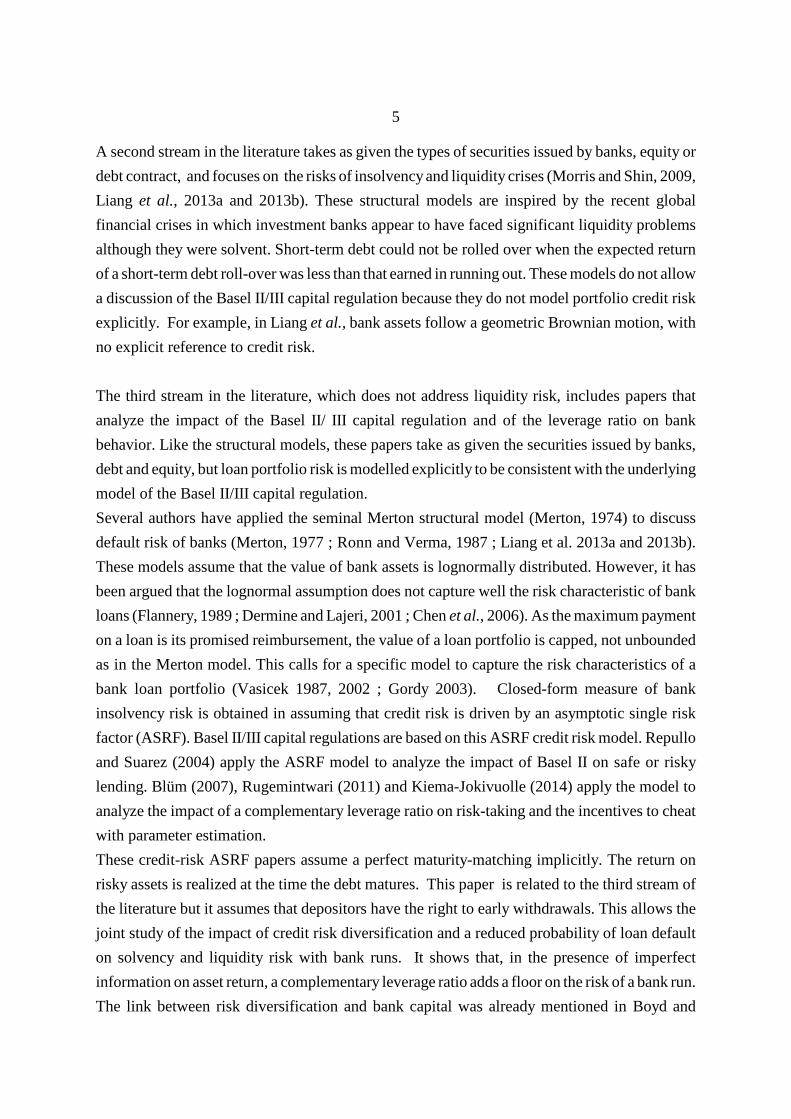
A second stream in the literature takes as given the types of securities issued by banks, equity or

debt contract, and focuses on the risks of insolvency and liquidity crises (Morris and Shin, 2009,

Liang et al., 2013a and 2013b). These structural models are inspired by the recent global

financial crises in which investment banks appear to have faced significant liquidity problems

although they were solvent. Short-term debt could not be rolled over when the expected return

of a short-term debt roll-over was less than that earned in running out. These models do not allow

a discussion of the Basel II/III capital regulation because they do not model portfolio credit risk

explicitly. For example, in Liang et al., bank assets follow a geometric Brownian motion, with

no explicit reference to credit risk.

The third stream in the literature, which does not address liquidity risk, includes papers that

analyze the impact of the Basel II/ III capital regulation and of the leverage ratio on bank

behavior. Like the structural models, these papers take as given the securities issued by banks,

debt and equity, but loan portfolio risk is modelled explicitly to be consistent with the underlying

model of the Basel II/III capital regulation.

Several authors have applied the seminal Merton structural model (Merton, 1974) to discuss

default risk of banks (Merton, 1977 ; Ronn and Verma, 1987 ; Liang et al. 2013a and 2013b).

These models assume that the value of bank assets is lognormally distributed. However, it has

been argued that the lognormal assumption does not capture well the risk characteristic of bank

loans (Flannery, 1989 ; Dermine and Lajeri, 2001 ; Chen et al., 2006). As the maximum payment

on a loan is its promised reimbursement, the value of a loan portfolio is capped, not unbounded

as in the Merton model. This calls for a specific model to capture the risk characteristics of a

bank loan portfolio (Vasicek 1987, 2002 ; Gordy 2003). Closed-form measure of bank

insolvency risk is obtained in assuming that credit risk is driven by an asymptotic single risk

factor (ASRF). Basel II/III capital regulations are based on this ASRF credit risk model. Repullo

and Suarez (2004) apply the ASRF model to analyze the impact of Basel II on safe or risky

lending. Blüm (2007), Rugemintwari (2011) and Kiema-Jokivuolle (2014) apply the model to

analyze the impact of a complementary leverage ratio on risk-taking and the incentives to cheat

with parameter estimation.

These credit-risk ASRF papers assume a perfect maturity-matching implicitly. The return on

risky assets is realized at the time the debt matures. This paper is related to the third stream of

the literature but it assumes that depositors have the right to early withdrawals. This allows the

joint study of the impact of credit risk diversification and a reduced probability of loan default

on solvency and liquidity risk with bank runs. It shows that, in the presence of imperfect

information on asset return, a complementary leverage ratio adds a floor on the risk of a bank run.

The link between risk diversification and bank capital was already mentioned in Boyd and

6

Runkle (1993) who argued that the benefits of risk diversification on the probability of default

of a bank can be zero if they are offset by a reduction of capital. These authors do not model

credit risk and assume implicitly that assets are funded with matched-maturity funding. The

novelty of our paper is to introduce liquidity risk and the probability of a bank run in the Basel

framework and to model credit risk diversification explicitly.

2. Bank Assets and Portfolio Credit Risk

In the spirit of the Basel capital regulation, we consider a one-period, say one year, model. A

loan portfolio is funded with deposits and equity. This section focuses on the asset side. The loan

portfolio model is based on the parsimonious presentation by Repullo and Suarez (2004). The

outcome of the model is identical to that of a Vasicek-Merton type approach in which bankruptcy

of a borrower occurs when the value of its lognormally distributed assets falls below a threshold

value (Merton, 1974, Vasicek, 1987). A bank lends to many firms indexed by i = 1....N. The

success or default of firm i is determined by a latent random variable Xi.. The case of default and

no-default by a borrower is given by the following rule:

No-default if Xi # 0

Default if Xi > 0

The latent variable Xi is defined as the sum of three terms:

X Fi i i i i= + + −µ ρ ρ ε( ) ( )1 1

with µi the expected value of Xi, F a single risk factor that affects all firms (a standardized

normally distributed variable), ρi a measure of the exposure of the firm to the systematic risk

factor F, and εi an economic shock specific to the firm (normally and independently distributed

with mean of 0 and standard deviation of 1). F is referred to as the systematic risk factor, ρi as

the factor-loading, and εi as a firm-specific or idiosyncratic shock. F can be interpreted as the

inverse of a macro-economic index. A high value implies a recession (large probability of

default), and a low value implies an expansion (low probability of default). In this section, loans

are homogeneous, so that the subscript i will be dropped for the expected value µ and the

correlation ρ. In Section 6, the results are extended to the more general case of a portfolio which

includes loans with different probabilities of default. In a homogeneous loan portfolio, it can be

shown that ρ is the correlation between the latent variables for firms i and j (Düllmann and

7

Masschelein, 2007). Finally, everything is lost in case of loan default.

Then, denote:

N: cumulative normal distribution

IN: Inverse cumulative normal distribution

For a given value of the systematic factor F, one can compute the conditional probability of

default of the homogeneous firm, p(F), PD denoting the unconditional probability of loan

default:

p F X

FN

F

NIN PD F

i

i

( ) ( )

( ) ( )

(( )

( )) ( )

= >

= > −+

−=

+−

=+

−

Probability

Probability

0

1 1

12

εµ ρ

ρµ ρ

ρ

ρρ

This result follows from properties of the symmetric normal distribution:

- For any constant c, Probability (εi > - c) = N (c)

- Unconditional probability of loan default = PD = Probab. (Xi > 0) = Pr (Xi - µ > - µ)

= N (µ)

It implies: µ = IN (PD)

Since the idiosyncratic terms ε i are independent and if the number of loans in the portfolio is

large, the Law of Large Numbers ensures that the percentage frequency of defaults in a loan

portfolio conditional on a given value of the factor F is equal to the conditional probability of

default. The maximum loss that one can face on a loan portfolio with α degree of confidence,

Credit-VAR, can be calculated by setting the systematic risk factor F equal to the α-quantile of

its distribution.

CreditVAR Default frequency confidencelevel for factor F

NIN PD IN

( ) ( )

(( ) ( )

( )) ( )

α α

ρ αρ

=

=+

−13

8

Basel II fixes capital to cover loan losses with a 99.9% confidence level. This model, referred

to as the asymptotic single risk factor (ASRF) model, permits one to calculate the aggregate loss

distribution on a loan portfolio. A useful property of the single risk factor model is the additivity

of risks. To calculate regulatory capital, the loan portfolio is divided into separate buckets of

loans, each with its own unconditional probability of default (PD). Capital is allocated to each

bucket to cover Credit-VAR, and regulatory capital is the sum of the bucket-based capital.

Credit-VAR is positively related to the correlation coefficient, ρ. A large correlation implies that

the likelihood of occurrence of joint or clustered defaults increases.

The Credit-VAR given by equation (3) is a loss conditional on a specific value for the systematic

risk factor F. One can compute (see Appendix 1) the unconditional cumulative probability

distribution function of the percentage of defaulted loans in a portfolio, L:

Probability ( ; ; )( ) ( )

( )L x PD NIN x IN PD

< =− −

ρ

ρρ

14

Relations (3) and (4) hold for large portfolios of loans, an assumption taken in the paper. Figures

1a and 1b show the loan loss distribution density for a PD of 2% and correlations of 0.03 and 0.1.

The probability distribution is highly skewed and leptokurtic (Vasicek, 2002). One observes that

a larger correlation (ρ = 0.1 vs. ρ = 0.03) pushes the probability mass in the two tails of the

distribution, with an increased probability of low rate or high rate of default clustering.

Insert Figures 1a ad 1b

3. Deposit Funding, Imperfect Information, and the Risk of Bank Run

Funding illiquid loans with short-term uninsured deposits introduces the risk of a bank run, a

disorderly outcome with depositors attempting to withdraw their funds. Uninsured depositors

could include large wholesale depositors the major source of bank runs in the United States

during the global financial crisis (Morris and Shin, 2009). Two outcomes at the end of the period

are possible. In the good one, loans mature and depositors are repaid. In the bad one, depositors

run to the bank to be the first in line to be repaid in full. As it is a one period model, we do not

explicitly model the consequence of a bank run but assume that it is a bad disorderly outcome.

9

The time sequence is as follows:

At the start of the year, the bank chooses an infinitely granular homogeneous one-year-to-maturity

loan portfolio. In the spirit of the Basel II capital regulation, discussed in section 2, loans are

characterized by the unconditional probability of loan default (PD) and the correlation (ρ). Due

to opacity, depositors do not know the characteristics of the loan portfolio. Once PD and ρ are

set, the level of capital is fixed by the regulator. Actions by the bank are taken at the start of the

period. No further action -such as a gamble for resurrection or equity issue - takes place.

The event of a bank run would unfold as follows. Before the maturity date of loans (the interim

period), information on loan losses filters out. It could be a rumor or periodic information

released by management. Depositors may run in the hope to be the first in line to avoid the

consequence of a bank default. Risk-neutral depositors will run if the expected payoff in the case

of a run dominates the expected payoff of a passive strategy. In this model, individual depositors

ignore the negative consequences of a collective bank run. The focus of the paper is on the

probability of a bank run, not on the costs arising from a disorderly ending.

The interpretation of a bank run in this one-period model deserves some explanation. As the bank

carries no liquid assets, it can only start to repay depositors after loans have been paid back. No

level of contingency liquid assets can help in this model (except a 100% coverage and the

negation of the bank function of funding illiquid loans with short-term deposits), as all uninsured

depositors will run if they fear a default of the bank. So, the good orderly outcome is having

depositors coming at any time during day t = 1 to collect their money after loans have been paid

back. The bad disorderly outcome, the bank run, is having all depositors queuing at the door

before the opening of the bank in the hope that the first in line will be repaid in full.

Depositors run as soon as the signal, the reported loan losses Lr, reaches an amount equal to

capital reduced by a margin factor to be defined. There are two potential reasons as to why

depositors will run before the capital is fully depleted. The first reason, in the spirit of Postlewaite

t = 0 (loan origination) interim (t < 1) t = 1 (loan maturity)Bank chooses correlation (ρ) Imperfect information on loan Loans matureand probability of loan default (PD). losses filters out. Risk of a and actual losses areCapital (C) is set by the regulator. bank run. evaluated.

10

and Vives (1987) or Liang et al. (2013a and 2013b), is the fear that an early liquidation (firesale)

of bank assets will create a loss of value. Even if depositors know that the actual value of losses

is lower than capital and that, collectively, they should not run to withdraw deposits, there is a

coordination problem, akin to a Prisoner’s dilemma. Depositors run, hoping to be the first in the

line to avoid the costs resulting from an early closure of the bank and the sale of illiquid assets.

An alternative scenario as to why a run occurs before the depletion of capital is due to imperfect

information. Depositors believe that the reported loan losses are equal to the actual amount of

realized loan losses plus some random noise. This is the scenario adopted in this paper. The

assumption of imperfect information on the solvency of a bank is often justified by the opacity or

complexity of transactions (Morgan, 2002 ; Gorton, 2013) or by the fact that banks’ accounts are

audited at discrete time intervals. The Asset Quality Reviews conducted by the troïka (IMF, ECB

and EU) in Portugal, Ireland, Greece and Spain and by the ECB for the euro-zone banks in 2014

are justified by the need to improve transparency and reduce doubts on the solvency of European

banks. In our model, it is essential that a bank run starts at a level of loan losses which is smaller

than the capital of the bank.

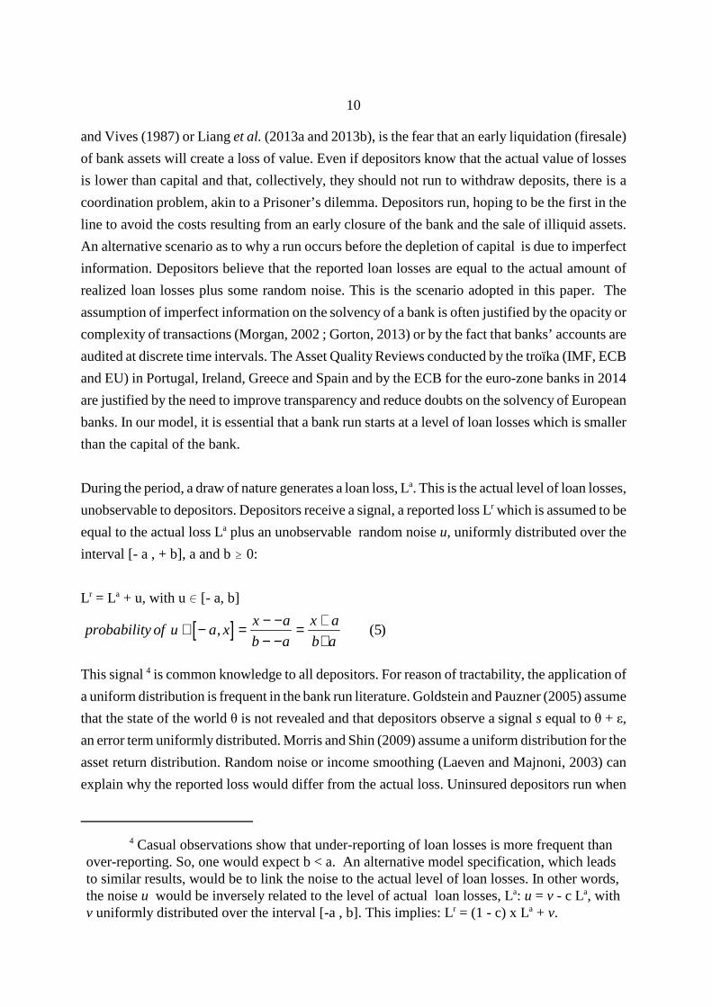
During the period, a draw of nature generates a loan loss, La. This is the actual level of loan losses,

unobservable to depositors. Depositors receive a signal, a reported loss Lr which is assumed to be

equal to the actual loss La plus an unobservable random noise u, uniformly distributed over the

interval [- a , + b], a and b $ 0:

Lr = La + u, with u 0 [- a, b]

[ ]probability of u a xx a

b a

x a

b a∈ − = − −

− −= +

+, ( )5

This signal 4 is common knowledge to all depositors. For reason of tractability, the application of

a uniform distribution is frequent in the bank run literature. Goldstein and Pauzner (2005) assume

that the state of the world θ is not revealed and that depositors observe a signal s equal to θ + ε,

an error term uniformly distributed. Morris and Shin (2009) assume a uniform distribution for the

asset return distribution. Random noise or income smoothing (Laeven and Majnoni, 2003) can

explain why the reported loss would differ from the actual loss. Uninsured depositors run when

4 Casual observations show that under-reporting of loan losses is more frequent thanover-reporting. So, one would expect b < a. An alternative model specification, which leadsto similar results, would be to link the noise to the actual level of loan losses. In other words,the noise u would be inversely related to the level of actual loan losses, La: u = v - c La, withv uniformly distributed over the interval [-a , b]. This implies: Lr = (1 - c) x La + v.

11

the reported loss Lr exceeds a threshold level Lr* to be defined. In Appendix 2, an imperfect

information model based on limited sampling of loans is shown to lead to similar results.

4. The Probability of a Bank Run

When depositors receive interim information on the level of loan losses Lr, they may decide to run

to be the first in line to collect money. One needs first to compute the threshold level of reported

loss Lr* leading to a bank run. The probability of a bank run is then the probability of receiving a

reported loss higher than this threshold value.

Threshold value of reported loss L r* leading to a bank run

Assume first that depositors have perfect information on the state of default/no default of the

bank. We show that if there is default, all depositors run because the expected payoff is higher

than in the no-run case. The expected payoffs for a depositor who assumes that all other depositors

run are given in Exhibit 1. Denote by A the value of bank’s assets at the end of the period, n the

number of depositors, and B the promised reimbursement per deposit (principal plus interest).

Default ( A < n x B) No-Default (A $ n x B)

Run B x A/(n x B)

+ (1 - A/(n x B) x (Max (A - (n-1) x B, 0))

B

No-Run Z = Max (A - (n-1) x B, 0) B

Exhibit 1 Expected payoffs for a depositor assuming all other depositors (n-1) run

If the bank is solvent, it is able to repay fully the promised amount B to each depositor. If there

is a default (A < n x B) and a bank run, the bank must follow a sequential service constraint and

it pays B until it runs out of resources. Assume the case of default and, as a start, that the depositor

believes that all other depositors (n - 1) will run. If she does not withdraw funds, she gets Z (either

zero or, if the assets A is large enough to pay the (n-1) depositors who run, the residual asset

value). If she runs, the expected return will be the payout B times the probability of being among

the first in the line that get paid (A/ (n x B)) plus the probability of not being paid (1 - A/(nxB))

times the payoff Z in case of being late in the line. The expected payoff in case of a run exceeds

the payoff of no-run:

[B x A/(n x B)] + [Z x (1 - A/(n x B))] > Z as B > Z (6)

12

If the belief that the number of runners is smaller than n-1, the incentive to run increases as the

probability of being paid is higher. As a consequence, in case of default and perfect information

on bank solvency, there is a unique equilibrium and all depositors run.

The above reasoning has assumed perfect information on solvency. With imperfect information

on the actual level of loan losses and common knowledge on the reported loss Lr, depositors will

compute the posterior probability (π) of actual losses as follows. Since the reported loss Lr is equal

to the actual loss La plus a random nooise u, uniformly distributed over the interval [- a, b], it

follows that, conditional on observing a reported loss Lr, the posterior probability of La is

uniformly distributed over the interval [Lr - b, Lr + a] (Goldstein and Pauzner, 2005). Depositors

will run if the posterior probability of default is positive as the expected payoffs of a run

dominates:

π x [ (B x A/(n x B)) + (Z x (1 - A/(n x B))] + (1 - π) x B > π x Z + (1 - π) x B

B x A/(n x B) + Z x (1 - A/(n x B)) > Z because B > Z (7)

Having demonstrated that a run will take place if the posterior probablity of default π is positive,

we calculate the threshold level of reported loss Lr* which generates a positive posterior

probability of default. Since the posterior probability of La is uniformly distributed over the

interval [Lr - b, Lr + a], it will be positive whenever the upperbound of the uniform distribution

is larger than the capital of the bank:

Lr + a > C (8)

It follows that the threshold value Lr* leading to a bank run is equal to C - a.

Probability of a Bank Run

The probability of a bank run is the probability of receiving a loss signal Lr exceeding the

threshold Lr*. Several critical values for actual losses La are reported below.

C - a - b C - g C - a C Actual Losses = La

13

Three regions of actual loan losses La have to be distinguished:

- For actual losses La < C - a - b, the probability of a run is zero (even if the noise takes the

highest value b, the reported loss Lr will be smaller than the threshold value Lr* ).

- For actual losses La > Capital, the probability is 1 (even if the noise takes the lowest value - a,

the reported loss Lr will be larger than the threshold).

- For actual losses La 0 [C - a - b, C], the probability of a run is the probability of u, such that

Lr = La + u > L r* = C - a. For example, if La = C - g (with a< g < a + b) is realized, we need a

signal

u > g - a , with a probability = (b - g + a)/(b + a).

The probability of a bank run can be calculated with the probability distribution of actual loan

losses. It is equal to the probability of La > C, plus the joint probability of L a 0 [C -a - b, C] and

u being a run noise. Since the noise u is independent of the actual loss, the joint probability can

be estimated. One segments the interval [C - a - b, C] into many sub-intervals, and multiplies the

probability of having an actual loan loss in a sub-interval by the probability of receiving the

necessary noise for a run.

The probability of a bank run is related to the probability distribution of actual loan losses, to the

degree of imperfect information, and to the level of capital. This is discussed next.

5. Probability of Loan Default, Portfolio Credit Risk, and Probability of Bank Runs: The Case

of Homogeneous Loans

For clarity of exposition, it is assumed in this section that loans are homogeneous. In Section 6,

the results are extended to the more general case of a portfolio of heterogenous loans.

Portfolio credit risk is chosen by the bank, capital is set by regulators under Basel II/III rule and

the probability of a run is calculated. One can then analyze the impact of a change of correlation

or loan probability of default on the probability of a run.

At t = 0, the bank chooses the type of portfolio credit risk which is related to default correlation

(ρ) and probability of loan default (PD). Some banks might be tempted to reduce costly capital

by choosing, ceteris paribus, the lowest available correlation in the market, ρmin > 0. Bank capital

could be costly because of information asymmetry (Bolton and Freixas, 2000) or one can refer to

14

a Modigliani-Miller corporate tax argument. A smaller correlation implies a reduced probability

of default clustering, and a reduced probability mass in the right tail of the loan loss distribution.

Correlation reduction is, in a credit risk context, synonymous with credit risk diversification,

understood as a reduction of the probability of default clustering. A floor on diversification, ρmin,

could be caused by a need to focus on profitable operations (Acharya et al., 2006). Other banks

could follow a different strategy when the profit of a focused portfolio outweighs the benefits of

diversification and lower capital. The purpose of our paper is not to discuss the choice of portfolio

credit risk but to introduce liquidity risk and to call the attention to the fact that a decrease in

default correlation or in the probability of loan default which is accompanied by a Basel Pillar 1

capital decrease will raise the probability of a bank run.

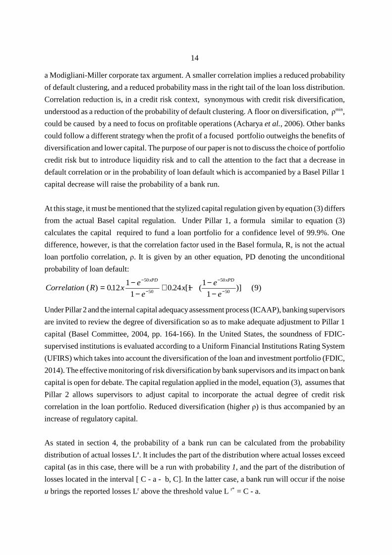
At this stage, it must be mentioned that the stylized capital regulation given by equation (3) differs

from the actual Basel capital regulation. Under Pillar 1, a formula similar to equation (3)

calculates the capital required to fund a loan portfolio for a confidence level of 99.9%. One

difference, however, is that the correlation factor used in the Basel formula, R, is not the actual

loan portfolio correlation, ρ. It is given by an other equation, PD denoting the unconditional

probability of loan default:

Correlation R xe

ex

e

e

xPD xPD

( ) . . [ ( )] ( )= −−

+ − −−

−

−

−

−0121

10 24 1

1

19

50

50

50

50

Under Pillar 2 and the internal capital adequacy assessment process (ICAAP), banking supervisors

are invited to review the degree of diversification so as to make adequate adjustment to Pillar 1

capital (Basel Committee, 2004, pp. 164-166). In the United States, the soundness of FDIC-

supervised institutions is evaluated according to a Uniform Financial Institutions Rating System

(UFIRS) which takes into account the diversification of the loan and investment portfolio (FDIC,

2014). The effective monitoring of risk diversification by bank supervisors and its impact on bank

capital is open for debate. The capital regulation applied in the model, equation (3), assumes that

Pillar 2 allows supervisors to adjust capital to incorporate the actual degree of credit risk

correlation in the loan portfolio. Reduced diversification (higher ρ) is thus accompanied by an

increase of regulatory capital.

As stated in section 4, the probability of a bank run can be calculated from the probability

distribution of actual losses La. It includes the part of the distribution where actual losses exceed

capital (as in this case, there will be a run with probability 1, and the part of the distribution of

losses located in the interval [ C - a - b, C]. In the latter case, a bank run will occur if the noise

u brings the reported losses Lr above the threshold value L r* = C - a.

15

Formally:

[ ]Probability Probability

Joint probability La

of run L C

C a b C and u such that L L u L C a

a

r a r

= >

+ ∈ − − = + > = −

( )

( , ) ( )* 10

with capital C given by Basel II/III capital regulation (equation 3) with α confidence.

The impact of diversification (reduction in correlation ρ) and probability of loan default on the

risk of a bank run can be analyzed. As there is no closed form solution for the impact of

correlation on the probability of a bank run (equation (10)), we calculate the probability of a bank

run with different degrees of correlation, probability of loan default and confidence level.

The range of correlations is 0.1 to 0.3, in line with the empirical literature.5 The unconditional

probabilities of loan default (PD) range from 0.5% (A-rated asset equivalent) to 2% (probability

of default observed in some SME sectors). The confidence level α is set at two levels, 99% and

99.9%, and the noise range [- a, b] set at [- 1%, + 1%]. In the absence of empirical information

on the magnitude of opacity, a small support is chosen for the noise: +/- 1% of the actual value

of assets. It is large enough to create a significant risk of bank run. The level of regulatory bank

capital and the probability of a bank run, based on equations (3) and (10), are given in Tables 1

and 2.

Insert Tables 1 and 2.

Since, due to imperfect information about the actual level of loan losses, a bank run starts before

capital is depleted, the probability of a bank run is greater than the confidence level set by the

regulator (under an implicit assumption of matched-maturity funding with no possibility of a run).

For example in Table 1, in the case of a correlation of 0.3 and an unconditional probability of loan

default (PD) of 0.5%, the probability of a bank run is 1.42%, while the confidence level for capital

was set at 99% with a 1% probability of bank default. The interesting result of Table 1 is how the

probability of a bank run varies when diversification and probability of loan default change. One

observes that, in all cases, a lower default correlation (increased diversification) increases the

probability of a bank run, although the Basel Pillar 1 capital regulation ensures a constant

5Basel II uses a correlation range of 0.12 to 0.24. Düllmann K. and N. Masschelein(2007) reports a correlation of 0.09 for German SMEs. Amato J. and Gyntelberg J.(2005)refer to an empirical correlation range of 0.05 to 0.3.

16

probability of default. For example, in Table 1 with the capital set for a confidence level of 99%,

the probability of a bank run increases from 1.42% to 5.7% when correlation is reduced from 0.3

to 0.1 for the low-risk loan with an unconditional probability of default (PD) of 0.5 %. In Table

2, with the capital set for a confidence level of 99.9%, the probability of bank run increases from

0.12% to 0.34% when correlation is reduced from 0.3 to 0.1 for the low-risk loan with a PD of

0.5%. A second observation is that, keeping correlation constant, the risk of a bank run increases

as one reduces the unconditional probability of default on loans, PD. For example in Table 1, with

a correlation of 0.1, the probability of a bank run increases from 1.7% to 5.7%, when the

unconditional probability of loan default is reduced from 2% to 0.5%.

One can observe that binding Basel II/III capital regulation aimed at a fixed probability of default

over a one-year period will, under imperfect information about the actual level of loan losses,

result in a probability of a bank run which is inversely related to correlation (diversification) and

to the probability of loan default. Note that periods of low correlation and low probability of loan

default are characteristics of economic prosperity. The literature on the procyclicality of Basel

II and on the variations in probability of loan default and correlation argues that they decrease in

periods of prosperity (Das et al., 2006 and 2007 ; Repullo and Suarez, 2013).

The intuition beyond the impact of correlation (and probability of loan default) on the probability

of a bank run is as follows. Remember that capital is set to ensure a constant probability of bank

default (loan losses exceeding capital with, let us say, a maximum 1% probability). So, what

explains the variations in the probability of a bank run for different correlation level, is the

variations in the probability of having actual loan losses located in the interval [C - a - b, C]. As

mentioned above, a higher correlation increases the probability mass on the tails of the loan loss

distribution. There is a higher probability of default clustering on the right side of the loan loss

distribution (when one defaults, others are likely to default), and a higher probability of very few

defaults on the left side of the distribution (when one does not default, others are unlikely to

default). If capital was kept constant, a reduction of correlation would reduce probability mass

in the right tail and the risk of a bank run. But with Pillar 1 capital being reduced, the locus of

actual loans losses generating a bank run discussed in section 4 (La > C - a - b) is moved to the

left of the aggregate loan loss distribution, and given the shape and slope of the loan loss

distribution, to a zone with higher probability mass. Figure 2a presents the loan loss distribution

for a correlation of 0.1. In comparison with Figure 2b (correlation of 0.2), regulatory bank capital

is reduced from 7.53% to 4.68%, bringing the bank run interval before capital is depleted [C - a -

b, C] to a zone with higher probability mass. Since the noise u is uniformly distributed over the

support [- a, b], the increase in probability of bank run is due to the loan loss probability mass

17

in the interval [C - a - b, C].

Insert figures 2a and 2b

The probability of a bank run is related not only to the confidence level assumed for bank capital,

but also to the location of capital on the loan loss probability distribution. Higher probability mass

for loan losses close to the level of capital generates a greater risk of a bank run. With reference

to Boyd and Runkle (1993) who questioned the benefits of diversification on the probability of

bank default, it is not only the capital reduction that reduces the benefit of diversification, but also

the move of the ‘bank run locus’, the loan losses which can generate a bank run, to a higher

probability zone.

A discussion of the main assumptions driving the results follows. To capture the world of

imperfect information faced by depositors, it is assumed that they do not know the asset risk

distribution (PD, ρ) chosen by the bank and that the reported loan losses are equal to the actual

losses plus a random noise distributed over an interval [- a, b]. It is this ‘imperfect information’

interval which leads depositors to run before capital is depleted. The results of the paper then

follow. A comment can be made on the independent interval [- a, b]. One could argue that more

sophisticated depositors could receive information about a sample of loan transactions and infer

the likelihood of realized loan losses. Imperfect information would be based on the access to a

limited sample of loans, and the risk of a bank run would no longer be limited to a particular range

of actual loan losses, as any level of actual loan losses could generate, with some probability, a

sample with large loan losses that generates a bank run. In Appendix 2, we provide a model of

imperfect information due to limited sampling, and show that the main result of the model holds

completely. An increase in credit risk diversification, which leads to a reduction of bank capital

compatible with the Basel III rule, increases the risk of a bank run.

6. Probability of Loan Default, Portfolio Credit Risk, and Probability of Bank Runs: The

Case of Heterogeneous Loans

The discussion so far has considered a homogeneous loans portfolio, with all loans having an

identical probability of default and unique correlation. In this section, we show that the above

results apply fully to a heterogeneous portfolio with specific buckets having a different probability

of default. The proof builds on the additivity property of the asymptotic single risk factor model.

Consider a loan portfolio with S buckets (i = 1....S), each with its own PDi. For each bucket, the

18

capital, Ci , necessary to cover losses in the event of a risk factor F(α) is given by equation (3).

Since there is a single risk factor, the regulatory capital, C, is equal to the sum of the capital

allocated to each bucket:

Regulatory Capital C Cii

S

= ==∑

1

11( )

For a given common risk factor F, the percentage of losses in each bucket, Li, is given by equation

(3). The percentage of losses in the total portfolio, L, is the weighted sum of percentage losses in

each bucket, Li, weighted by the percentage loan allocation in each bucket ωi.

Total percentage loanlosses L L xii

S

i= ==∑

1

12ω ( )

For a specific loan portfolio, one can calculate the probability of a bank run. It works in three

steps.

With information on probability of default and correlation, one can compute the regulatory capital

Ci, applying equation (3) to each bucket. Regulatory capital is the sum of bucket-capitals. Next,

one simulates the level of aggregate loan losses for various values of the single risk factor F,

which allows to identify the bank run threshold value for the single risk factor, Frun, which is such

that aggregate loan losses are equal to the capital reduced by the margin factor a + b. Finally, one

computes the cumulative probability of having a single risk factor value that generates a bank run.

As in section 4, one will need to distinguish two cases: the case where risk factor F generates

actual aggregate losses higher than capital, thus making a run a certainty, and the second case

which involves a single factor F that generates losses in the interval [C- a- b, C]. A run will only

occur if the noise u leads to reported losses that generate a run (Lr > C - a). In the second case,

joint probabilities need to be calculated.

To illustrate this, we calculate in Table 3 the probability of a bank run for a balanced portfolio,

with 50% invested in loans with PD of 1%, and 50% in loans with PD of 2%. For ease of

exposition, we assume that an identical correlation ρ applies to each bucket. For a correlation

ranging from 0.3 to 0.1, one observes that the regulatory Basel II/III capital needed for a

confidence level of 99% moves from 14% to 6.46%, while the risk of a bank run increases from

1.19% to 1.97 %. This is similar to the results of section 5 (homogeneous loan portfolio) and

Tables 1 and 2. A lower correlation which allows a reduction of regulatory capital increases the

risk of a bank run.

Insert Table 3.

19

7. Optimal Regulation to Reduce the Risk of a Bank Run

To reduce the probability of a bank run to some confidence level, one could adjust the capital

regulation or one could impose constraints on the maturity mismatch. A discussion follows.

It was shown in section 5 that the regulatory capital reduction induced by diversification moves

the ‘bank run locus’ into a higher probability mass area. Consequently, it might be tempting to

make the capital regulation invariant to diversification. This would be the case with a strict

application of Basel II Pillar I, in which the correlation used in the formula, R, is given by

equation (9) which is not related to the the actual credit risk correlation. In Table 4, we report

the level of bank capital for a 99% confidence level for the case of the homogeneous loan

portfolio. The probability of a bank run is given by equation (10), in which the Basel capital is

given by equation (3) with correlation R given by equation (9).

Insert Tables 4 and 5.

For example, for a probability of default of 0.5%, one first observes that the level of capital,

4.53%, is invariant to change in correlation. A decrease in correlation from 0.3 to 0.1 reduces the

probability of a bank run from 2.62% to 0.37%. As explained above, a reduction of correlation

reduces the probability density in the right tail at around the level of capital, generating a

reduction of the probability of a bank run. However, since banks do not obtain a capital reduction

from diversification, they will have little incentive to reduce correlation. As shown in the

collaterized debt obligation literature (Gibson, 2004, and Hull and White, 2004), an increase of

correlation will benefit the equity tranche in cases where one can expropriate the senior tranche.6

This is the usual moral hazard problem reported in a Merton-type framework (Merton, 1977).

An optimal bank capital regulation should link capital to diversification and probabilities of loan

default, while controlling the risk of a bank run. In Table 5, we compute the capital necessary to

limit the probability of a bank run to 1%, for various levels of correlation and probability of loan

default. A comparison is made with the Basel pillar 1 capital allocation given in Table 1, which

was based on a 1% confidence level and a capital relief driven by diversification. For example,

6In the CDOs tranche literature, an increase in correlation benefit equity holders at theexpense of the senior tranche when the terms -CDS spreads- have been fixed ex ante.Expropriation occurs because correlation increases default clustering and losses born by thesenior tranche, while correlation also increases the probability of few defaults, benefiting theequity tranche.

20

for loans with PD of 0.5% and a correlation of 0.1, the level of capital needed to limit the

probability of a bank run to 1% should be 3.7%, compared to a Basel capital of 2.62%, a relative

difference of 37%. The intuition is that the Basel II/III capital must be increased so as to push it

to a region with smaller probability mass on the aggregate loan loss probability distribution.

Regulatory capital should consist of two parts: capital to cover actual losses with some

confidence level, and additional capital to cover the risk of a bank run due to imperfect

information. This last component is linked to the degree of imperfect information and to the shape

of the loss distribution which is driven by two parameters in this credit risk model: correlation and

probability of default.

Insert Figure 3

In Figure 3, we report Basel Pillar 1 capital and the capital needed to limit the risk of a bank run

to 1% for several probabilities of loan default ranging from 0.01% to 5%. As is apparent, a floor

on leverage is needed in the case of small probabilities of loan default. The model provides an

alternative justification for the supplementary leverage ratio. A leverage ratio, a floor on the

capital-to-assets ratio, is justified by the need to limit the risk of a bank run when there is

imperfect information on the value of a bank’s assets.

One could object that the FDIC supplementary leverage ratio requirement of 3% did not prevent

the 2007-2009 banking crisis. A first observation is that the crisis erupted in investment banks not

subject to FDIC regulations, Bear Stearns, Merrill Lynch and Lehman Brothers. A second

observation is that the leverage ratio did not take into account the implicit or explicit liquidity

lines given to loan securitization vehicles. When there was a run on the asset-backed commercial

paper market, banks were forced to refinance these assets (Covitz et al., 2013). The 3% leverage

ratio requirement might have been too low. In April 2014, the Federal Reserve Board, the FDIC

and the Office of the Comptroller of the Currency adopted a enhanced leverage ratio rule for the

largest interconnected U.S. banking organizations. Top-tier bank holding companies with more

than $700 billion in consolidated total assets must maintain a leverage ratio superior to 5% to

avoid restrictions on capital distribution and discretionary bonus payments. This rule will be

effective as of January 1, 2018 (Board of Governors, 2014).

An other way to limit the risk of bank run is to impose constraints on maturity mismatch and the

holding of liquid assets, such as the Basel III rule on the liquidity coverage ratio (LCR). The

liquidity coverage ratio (LCR) of Basel III forces banks to hold contingency liquid assets to cover

cash outflow in a 30-day stress scenario. As in our model, all uninsured depositors would run if

21

there is a fear of insolvency, the LCR would have to reach 100% of short-term deposits, making

the transformation of illiquid assets into liquid liabilities impossible. This model, which takes as

given the securities issued by banks, does not allow to evaluate the welfare cost of banning

liquidity transformation. One would need to rely on the fundamental economics stream of

banking literature, reviewed in Section 1, which endogenizes the types of securities. But this paper

shows that, if one accepts the function of maturity transformation, then a leverage ratio is needed

to reduce the risk of a bank run.

Conclusion

A credit risk-based model with short-term deposits and imperfect information about the actual

level of loan losses is presented in this paper. In a stylized Basel II/III capital regulation

framework, we study the impact of credit risk diversification and probability of loan default on

the probability of a bank run. In our model, depositors who do not know the asset risk distribution

chosen by the bank believe that actual loan losses could differ from reported loan losses. Imperfect

information about actual loan losses increases the risk of a bank run, calling for more capital. We

show that capital relief, which is induced by increased diversification or lower probabilities of

loan default, leads to a higher probability of a bank run. This is due to the nature of credit risk and

the shape/slope of the aggregate loan loss probability distribution. A reduction of capital displaces

the ‘bank run locus’ to a region with higher probability mass. The main result of the paper is

robust. In a second setting discussed in Appendix 2, a limited sampling of loans is the source of

imperfect information. It leads to the same conclusion.

A floor on leverage, an unweighted leverage ratio, is often justified by simplicity and

transparency, the avoidance of gaming the system, robustness to estimation errors or the need for

banks to have enough capital in case the economy deteriorates. Our model provides an additional

justification for a leverage ratio. In periods of economic prosperity characterized by low

probabilities of loan default and low correlation, a floor on leverage is needed to limit the risk of

a bank run. Additional policy tools, besides deposit insurance, to reduce the probability of a bank

run are the disclosure of credible information, the contractual option to extend maturity in a crisis,

a prompt and corrective action (PCA) procedure to increase capital rapidly and/or the access of

solvent banks to a central bank’s discount window. A strict application of a liquidity coverage

ratio with 100% backing by safe liquid assets will eliminate bank runs but also negate an

important function of banks, the creation of liquid claims on illiquid assets.

22

References

Acharya V.V., I. Hasan, and A. Saunders (2006): “ Should Banks be Diversified ? Evidence fromIndividual Bank Loan Portfolios ?”, Journal of Business, 79 (3), 1355-1412.

Allen F. and D. Gale (2007): Understanding Financial Crises, Oxford University Press.

Amato J.D. and J. Gyntelberg J.(2005): “CDS Index Tranches and the Pricing of Credit RiskCorrelations”, BIS Quarterly Review, March, 73-87.

Basel Committee on Banking Supervision (1988): “International Convergence of CapitalMeasurement and Capital Standards”, July, Bank for International Settlements, Basel.

Basel Committee on Banking Supervision (2004): “International Convergence of CapitalMeasurement and Capital Standards”, Bank for International Settlements, Basel.

Basel Committee on Banking Supervision (2010): Basel III: A Global Regulatory Framework forMore Resilient Banks and Banking Systems, December (revised June 2011), 1- 69 Bank forInternational Settlements, Basel.

Basel Committee on Banking Supervision (2013): “The Liquidity Coverage Ratio and LiquidityRisk Monitoring Tools”, January, 1-69, Bank for International Settlements, Basel.

Basel Committee on Banking Supervision (2014a): “Basel III: The Net Stable Funding Ratio”,Consultative Document, January, 1- 11, Bank for International Settlements, Basel.

Basel Committee on Banking Supervision (2014b): “Basel III Leverage Ratio Framework andDisclosure Requirements”, January, 1- 19, Basel Committee on Banking Supervision.

Board of Governors (2014): “Agencies Adopt Enhanced Supplementary Leverage Ratio FinalRule”, 8 April, http://www.federalreserve.gov/newsevents/press/bcreg/20140408a.htm.

Blum Jürg M.: “Why ‘Basel II’ May need a Leverage Ratio Restriction”, Journal of Banking andFinance, 32 (8), 1699-1707.

Bolton P. and X. Freixas (2000): “Equity, Bonds and Bank Debt: Capital Structure and FinancialMarket Equilibrium under Asymmetric Information”, Journal of Political Economy, 108 (2), 324-351.

Boyd J. and D. Runkle (1993): “Size and Performance of Banking Firms”, Journal of MonetaryEconomics, 47-67.

Bryant John (1980): “ A Model of Reserves, Bank Run and Deposit Insurance”, Journal of

23

Banking and Finance, 4, 335-344.

Chen A., N. Ju., S.C. Mazumdar, and A. Verma (2006): “Correlated Default Risks and BankRegulations”, Journal of Money, Credit and Banking, 38(2), 375-398.

Covitz D., N. Liang and G. Suarez (2013): “The Evolution of a Financial Crisis: Collapse of theAsset-Backed Commercial Paper Market”, Journal of Finance, vol. 68 (3) , 815 - 848

Dang Tri Vi , Gary Gorton and Bengt Holmström (2013): “Ignorance, Debt and Financial Crises”,mimeo, 1 - 34.

Das S. R., L. Freed, G. Geng and N. Kapadia (2006): “Correlated Default Risk”, Journal of FixedIncome, Fall, 7-32.

Das S.R., D. Darrell, N. Kapadia and L. Saita (2007): “Common Failings: How CorporateDefaults are Correlated “, Journal of Finance, 62(1), 93-117.

de Larosière J. (2009): “Financial Regulators must take Care over Capital”, Financial Times, 16October.

Dermine J. and F. Lajeri (2001): ”Credit Risk and the Deposit Insurance Premium, a Note”, Journal of Economics and Business, 53 (5), September/October 2001, 497-508.

Diamond, D. and P. Dybvig (1983): “Bank Runs, Deposit Insurance and Liquidity”, Journal ofPolitical Economy, 91, 401-419

Düllmann K. and N. Masschelein (2007): “A Tractable Model to Measure Sector ConcentrationRisk in Credit Portfolios”, Journal of Financial Services Research,, 32, 55-79.

FDIC (2014): FDIC Law, Regulations, Related Acts: Uniform Financial Institutions RatingSystem, https://www.fdic.gov/regulations/laws/rules/5000-900.html.

Financial Stability Forum (2009): “Report of the Financial Stability Forum on AddressingProcyclicality in the Financial System”, 2 April, 1-27.

Flannery M. (1989) : “Capital Regulation and Insured Banks’ Choice of Individual Loan DefaultRisks”, Journal of Monetary Economics, 24, 235-258.

Flannery M. and K.P. Rangan (2202): “Market Forces at Work in the Banking Industry: Evidencefrom the Capital Buildup in the 1990s”, mimeo.

Gibson M.S. (2004): “Understanding the Risk of Synthetic CDOs”, Federal Reserve BoardResearch papers 34, July, 1-27.

Goldstein Itay and Ady Pauzner (2005): “Demand-deposit Contracts and the Probability of BankRuns”, Journal of Finance 60 (3), 1293-1327.

24

Gordy M.B. (2003): “A Risk-Factor Model Foundation for Ratings-Based Bank Capital Rules”,Journal of Financial Intermediation, 12, 199-232.

Gorton D. (2013): “The Development of Opacity in U.S. Banking”, Yale Journal of Regulation,1-23.

Gorton Gary and George Pennachi (1990): “Financial Intermediaries and Liquidity Creation”,Journal of Finance XLV (1), 49 - 71. Haldane A.G. (2012): “The Dog and the Frisbee”, Federal Reserve Bank of Kansas City’s 36th

Economic Policy Symposium, The Changing Policy Landscape, Jackson Hole, Wyoming.

Hillier F.S. and G.B Lieberman (1974): Operations Research, San Francisco: Holden-Day, Inc.

Hull J. and A. White (2004): “ Valuation of a CDO and n-th to Default CDS Without Monte CarloSimulation”, Journal of Derivatives, 8-23.

Jacklin Charles and Sudipto Bhattacharya (1988): “Distinguishing Panics and Information-basedBank Runs: Welfare and Policy Implications”, Journal of Political Economy 96, 568-592.

Jarrow R. (2012): “A Leverage Rule for Capital Adequacy”, mimeo, Cornell University, 1-9.

Kiema Ikka and Esa Jokivuolle (2014): “Does a Leverage Ratio Requirement Increase BankStability?”, Journal of Banking and Finance, 39, 240-254.

Laeven Luc and Giovanni Majnoni (2003): “Loan Loss Provisioning and Economic Slowdowns:Too Much, Too Late”, Journal of Financial Intermediation, 12 (2), 178-197.

Liang Gechun, Lütkebohmert Eva and Yajun Xiao (2013): “A Multiperiod Bank Run Model forLiquidity Risk”, Review of Finance, 1 - 40.

Liang Gechun, Eva Lütkebohmert and Yajun Xiao (2013): “Funding Liquidity: Debt tenorstructure, and Creditor’s Belief: An Exogenous Dynamic Debt Run Model”, mimeo, 1 - 40.

Merton R. (1974): “On the Pricing of Corporate Debt: The Risk Structure of Interest Rates”,Journal of Finance, 34, 449-470.

Merton R. (1977):”An Analytic Derivation of the Cost of Deposit Insurance and LoanGuarantees”, Journal of Banking and Finance, 1, 3-11.

Mood A. and F. Graybill (1963): Introduction to the Theory of Statistics, 2nd edition, NewYork: McGraw-Hill.

Morgan D. (2002): “Rating Banks: Risk and Uncertainty in an Opaque Industry”, AmericanEconomic Review, 92, 874-888.

25

Morris Stephen and Hyun Song Shin (2009): “Illiquidity Component of Credit Risk”, mimeo,Princeton University, 1- 42.

Postlewaite A. and X. Vives (1987): “Bank Runs as Equilibrium Phenomenon”, Journal ofPolitical Economy, 95, 485-491.

Repullo R. and J. Suarez (2004): “Loan Pricing under Capital Requirement”, Journal ofFinancial Intermediation, 13 (4), 496-521.

Repullo R. and J. Suarez (2013): “The Procyclical Effects of Basel Capital Regulation”,Review of Financial Studies, 26, 452-490.

Ronn E.I. and A.K. Verma (1987 ): ”Pricing Risk-adjusted Deposit Insurance, an Option-basedModel”, Journal of Finance, 41, 871-895.

Rugemintwari Clovis (2011): “The leverage Ratio as Bank Discipline Device”, RevueEconomiue, 62 (3) 479-469.

Vasicek (1987): “Probability of Loss on Loan Portfolio”, Working Paper, KMV Corporation.

Vasicek (2002): “Loan Portfolio Value”, Risk, December, 160-162.

26

Appendix 1: Unconditional Loan Loss Distribution

The unconditional loan loss distribution for an infinitely granular homogeneous loan portfolio

is calculated in this section. It builds on Vasicek (2002). We start with the conditional Credit-

VAR given by equation (3):

Percentageof losses F F x NIN PD F

( ) (( )

( ))

_

_

= = =+

−ρ

ρ1

This yields:

IN PD FIN x

( )( )

_

+−

=ρ

ρ1

FIN x IN PD_ ( ) ( )

=− −1 ρ

ρ

Probability

Probability

( ) Pr ( ) ( )

( )( ) ( )

.

_ _

Loss x obability F F N F

Loss x NIN x IN PD

< = < =

< =− −

1 ρρ

27

Appendix 2: Bank run due to random sampling

In this paper, the bank run starts before capital is depleted by reported loan losses. The run is

caused by a belief of depositors that the reported level of loan losses is equal to the actual loan

losses plus some noise u distributed over an interval [- a, b]. This assumption captures the

intuition that depositors will run before capital is depleted.

An alternative scenario is as follows. Due to opacity, depositors do not know the probability

distribution of loan losses, PD and ρ. However, they are able to draw a random sample of n

loans at the interim date before the maturity of the loans.7 They observe the percentage of

defaulted loans in the sample, and estimate a confidence interval on the actual percentage of

defaulted loans in the portfolio. They run when the upper bound of the confidence interval on

loan losses exceeds the capital of the bank.

The unconditional probability of a bank run is equal to:

Probability (La 1 Bank run) = Probability La x Probability bank run# La

with La = actual percentage of loans in default.

Three types of data are required to evaluate the probability of a bank run: the probability

distribution of actual loan losses La, the probability of observing Lo defaults in the sample

given actual loan defaults La, and, given observing Lo, the computation of a confidence

interval on actual loan losses.

Consider a granular portfolio of homogeneous loans with probability of default PD and

correlation ρ. The unconditional cumulative probability distribution of the percentage of loans

in default is given in the paper by equation (4).

Let us assume that an actual percentage of loan defaults, La , is realized and that depositors

draw a sample of n loans from this large granular portfolio, observing a percentage of loans in

default Lo. Given an actual percentage of loans in default La, one can compute the probability

of observing Lo defaults out of a sample of n loans. This is an application of the statistics of

sampling (Hillier and Liebermann, 1974). The draw of a loan that shows either ‘in default’

7 ‘Drawing a sample’ is interpreted as receiving information about the status of nloans.

28

or ‘performing’ is a Bernouilli random variable. Since the n draws are independent (each loan

being taken out of a large granular portfolio), the probability of observing Lo loans in default

out of a sample of n loans is given by a binomial distribution:

Probability ( )!

!( )!number of defaults L

n

L n L L Lo

o o a

L

a

n Lo o

= =−

−

−1

11

For each actual realization La of a percentage of loans in default, one can compute the

probability of observing a percentage number of loans in default, Lo, in a sample of n loans.

The next step involves the calculation of a confidence interval for the actual percentage of

loans in default conditional on the observation of Lo defaulted loans in the sample. In the case

of a large sample for a binomial distribution, the two-sided 90% confidence interval for the

actual percentage of loans in default, La , can be approximated as follows (Mood and Graybill,

1963, p.263):

Probability[ .( )

.( )

]LL L

nL L

L L

no

o oa− − < < + − ≈1656

11656

190%0

0 0

The right side gives an upperbound on the actual percentage of loans in default, La, with a

one-side confidence level of 5%. In other words, there is 5% probability that the actual

percentage of loan losses exceeds the upperbound. We assume that depositors start to run

when the upper bound exceeds the capital of the bank, C. An infinite sample would lead to

perfect information with the observed Lo being equal to the actual percentage of loan losses La.

In line with the spirit of the paper, imperfect information, we will assume that the size of the

sample n is finite, leading to imperfect information about the actual level of loan losses.

A numerical example illustrates the procedure. Conditional on the (unobserved) realization of

actual loan default La of 1%, and the draw of a sample of 100 loans, one can compute the

probability of observing Lo default loans in the sample and estimate a confidence interval for

the actual percentage of loans in default by applying the binomial distribution and the 5%-one

sided confidence interval :

29

Observed frequency of

default, Lo, in a random

sample of 100 loans

Probability of Lo

(conditional on La = 1%)

5%-confidence upper bound

for La , conditional on L0

Lo = 0% 36.6% 0%

Lo = 1% 36.97% 2.64%

Lo = 2% 18.49% 4.30%

Lo = 3% 6.10% 5.81%

Lo = 4% 1.49% 7.22%

Lo = 5% 0.29% 8.59%

Lo = 6% 0.05% 9.91%

Lo = 7% 0.01% 11.2%

... ... ...

Probabilities of observing Lo defaulted loans and confidence interval on actual loan

losses La with a random sample of 100 loans and actual loan default rate La of 1%.

Applying the Basel II/III formula (2) for a 99% confidence level, capital would be set at 4.68%

in the case of a correlation of 0.1 and a PD of 0.1% (Table 6). Conditional on the unobserved

realization of La = 1%, one can calculate the probability of a run (all cases where Lo leads to a

confidence interval upper bound above the capital of 4.68%, that is for all Lo $3%). The

conditional probability of a run is directly related to the amount of capital and, therefore to

correlation. In the case of a realization of La = 1%, we calculate8 the conditional probability of a

run at 7.94% for a correlation of 0.1, and at 0.01% for a correlation of 0.3. The reason for the

significant reduction of the conditional probability of a run is that a higher correlation commands

a higher level of capital (10.43%), and a much reduced probability of the confidence interval

exceeding that capital.

To summarize, for a given level of actual loss (La), we can compute the probability of observing

a percentage of defaults in the sample, Lo, and its related confidence interval on the estimate of

actual loan losses. This allows us to compute the probability of a bank run conditional on a

8Calculations are available from the author upon request.

30

realization of actual loss La (all cases where the upperbound confidence interval exceeds the

capital).

In the final step, we discretize the probability distribution of actual loan losses La and take the sum

of the products of the probability of a realization of an actual loan loss La by the probability of a

bank run conditional on La. This gives the unconditional probability of a bank run in the economy:

Probability (La 1 Bank run) = Probability La x Probability Bank run# La

In Table 6, we report the probabilities of a bank run for a granular homogeneous loan portfolio

with a probability of loan default of 1%, and correlations ranging from 0.1 to 0.3.

Insert Table 6.

The capital is given by the Basel II formula (3) for a 99% confidence interval, identical to that

of Table 1. The economics of a bank run is now due to imperfect information resulting from a

limited sample size. As in the core of this paper, one observes that the unconditional probability

of a run increases with a reduction in correlation, from 3.17% in the case of a 0.3 correlation to

13.64% in the case of a 0.1 correlation. Two effects are at work. As indicated in section 2, a

higher correlation increases the probability mass at the extreme of the distribution. There is a

higher probability of a clustering of default cases. The second effect is that, conditional on the

realization of an actual percentage default, a higher correlation reduces substantially the

probability of a bank run because there is more capital. For a large correlation, the reduction in

the conditional probability of a run dominates the higher probability of having a large actual

default rate.

One can compare how imperfect information creates a bank run in the imperfect information

models presented in the paper and in this Appendix. A run can start in the paper as soon as the

actual loan losses exceed a threshold, C - a - b. Since the probability of losses exceeding capital

is the confidence interval set in Basel II (say 1%), the effect of correlation on the probability of

a run is due to its impact on the probability mass of La 0[C-a-b, C]. A reduction of capital due to

a lower correlation increases the probability mass for the bank run locus. In this appendix, the

dynamics are different. A run can occur for any value of actual losses La. Conditional on a realized

loss La, a sample is drawn, and a run occurs if the upper bound of the confidence interval on losses

exceeds the capital. As a lower correlation reduces capital, it increases the conditional probability

31

of a bank run. In both models, it is the capital reduction, induced by credit risk diversification,

which increases the risk of a bank run.

32

Figure 1a Loan loss density function (Vasicek, 2002)

0% 2% 5% 7% 10%

Figure 1b Loan loss density function (Vasicek, 2002)

0% 2% 5% 7% 10%

33

Figure 2a

Figure 2b

Note: Loan Loss Density Function reporting the probability of observing x% of the loan portfolioin default (Vasicek, 2002). Bank capital ( C) is set to cover loan losses with a confidence level of99%. The level of actual loan losses, C -a - b, represents the threshold over which a bank runcould take place.

0% 2% 5% 7% 10%

C-a-b C = Capital99%confidence : 4.68%

0% 2% 5% 7% 10%

C-a-b C = Capital99%confidence : 7.53%

34

Figure 3: Capital needed to limit the risk of a bank run to 1%. PD is the unconditionalprobability of loan default. The continuous line reports the Basel II/III capital for aconfidence level of 99%. The broken line reports capital needed to ensure a risk of bank runof 1%. The correlation is set at 0.1.

0

0.02

0.04

0.06

0.08

0.10

0.12

0.14

0.16

0.18

0,01% 0,10% 0,50% 1,00% 2,00% 5,00%

35

Table 1: Regulatory capital and probability of bank run. Basel II Capital is calculated withequation (3) for a confidence level of 99%. Probability of a bank run is calculated withequation (10), assuming that the noise u is distributed over the interval [-1%, +1%]. PD =Unconditional probability of loan default.

PD = 0.5% PD = 1% PD = 2%

Correl. Capital(%)

Prob. Run(%)

Capital (%)

Prob. Run(%)

Capital(%)

Prob. Run(%)

0.1 2.62 5.7 4.68 2.47 8.24 1.7

0.2 4.3 1.91 7.53 1.46 12.86 1.28

0.3 5.99 1.42 10.43 1.24 17.57 1.16

Table 2: Regulatory capital and probability of a bank run. Capital is calculated withequation (3) for a confidence level of 99.9%. Probability of a bank run is calculated withequation (10), assuming that the noise u is distributed over the interval [-1%, +1 %]. PD =Unconditional probability of loan default.

PD = 0.5% PD = 1% PD = 2%

Correl. Capital(%)

Prob. Run(%)

Capital (%)

Prob. Run(%)

Capital(%)

Prob. Run(%)

0.1 4.6 0.34 7.45 0.21 12.82 0.16

0.2 9.1 0.15 14.55 0.13 22.63 0.12

0.3 14.56 0.12 22.44 0.12 33.3 0.11

36

Table 3: Regulatory capital and probability of a bank run for a heterogeneous portfolio ofloans with different PDs. The portfolio of loans is balanced with 50% of loans with PD =1%, and 50% with PD = 2%. Capital for each bucket is calculated with equation (3) for aconfidence level of 99%. The value of risk factor F is calculated with equation (3) to ensurea loss equal to the capital reduced by a margin (a + b). The random noise u is assumed tobe distributed over the interval [-1%, + 1%].

Correlation Regulatory Capital Probability of Bank Run

0.1 6.46% 1.97 %

0.2 10.19% 1.36 %

0.3 14.00% 1.19 %

Table 4: Regulatory capital and probability of a bank run. Capital is calculated withequation (3) for a confidence level of 99%, and a constant correlation given by the Basel IIformula (9). Probability of a bank run is calculated with equation (10), assuming that therandom noise u is distributed over the interval [-1%, +1 %]. PD = Unconditional probabilityof loan default.

PD = 0.5% PD = 1% PD = 2%

Correl. Capital (%)

Prob. Run(%)

Capital(%)

Prob. Run(%)

Capital(%)

Prob. Run(%)

0.1 4.53 0.37 7.32 0.29 11.21 0.36

0.2 4.53 1.64 7.32 1.59 11.21 1.98

0.3 4.53 2.62 7.32 2.76 11.21 3.48

37

Table 5. Capital needed to ensure a probability of a bank run of 1%, compared to BaselPillar 1 capital necessary to ensure a probability of default of 1%. Probability of a bank runis given by equation (10) with a random noise u assumed to be distributed over the interval [-1%, +1%]. PD = Unconditional probability of loan default.

PD = 0.5% PD = 1% PD = 2%

Correl. CapitalBasel II

99%

Capitalensures a

Probabilityof bank

runof 1%

CapitalBasel II

99%

Capitalensures a

Probabilityof bank

runof 1%

CapitalBasel II

99%

Capitalensures a

Probabilityof bank run

of 1%

0.1 2.62 3.7 4.68 5.7 8.24 9.2

0.2 4.3 5.3 7.53 8.5 12.86 13.9

0.3 5.99 7.0 10.43 11.4 17.57 18.5

Table 6: Regulatory capital and probability of a bank run. Capital is calculated withequation (3) for a confidence level of 99%. Probability of a bank run is calculated asdescribed in the Appendix 2 for a random sample of 100 loans and a one-side confidenceinterval level of 95%. PD = Unconditional probability of loan default.

PD = 1%

Correl. Basel II Capital (%) Prob. Run (%)

0.1 4.68 13.64

0.2 7.53 5.89

0.3 10.43 3.17