Bargaining Micro-foundations of DecentralizedMarkets, Competition, and Reputation

Ashutosh Dinesh Thakur

Advisor: Dilip Abreu

April 12, 2014

Submitted to Princeton UniversityDepartment of Economics

In Partial Fulfilment of the Requirements for the A.B. Degree.

Acknowledgements

To my parents, for their love, blessings, and support in all that I ever wanted to pursue. I amgrateful to my family— Bhaikaka, Maiaaji, Bhai, Jiji, Ajoba, Aaji, and Aditya—for their encour-agement and blessings. I would like to particularly thank my thesis adviser, mentor, and teacher,Professor Dilip Abreu, for his guidance and patience, and my mentor and teacher, Professor MatiasIaryczower, who not only fostered my interest in game theory, but also introduced me to Abreuand Gul (2000) in POL 576, leading to this thesis topic. A special thanks to my graduate studentfriends Nemanja Antic, Rohit Lamba, Olivier Darmouni, Juha Tolvanen, Alexander Rodnyansky,and Pathikrit Bhattacharya. I am forever indebted to these and all other faculty, graduate students,and dear colleagues for making my time at Princeton such an instructive, enjoyable, and memorableexperience.

BARGAINING MICRO-FOUNDATIONS OF DECENTRALIZED

MARKETS, COMPETITION, AND REPUTATION

ASHUTOSH THAKUR

Abstract. Existing literature shows that it is possible for rational players to establish one-sided

and two-sided reputation in a bilateral bargaining environment by mimicking irrational, r -insistent

players, and that this reputation build-up can drastically change the Rubinstein (1982) outcome,by causing delay in reaching agreement. Furthermore, the literature on outside options in bilateral

bargaining suggests that unless outside options are very large, they do not affect these bargainingoutcomes. We are interested in the impact on the bargaining outcome from endogenizing outside

options—namely, bargaining in markets. In the presence of competition in decentralized search

markets, can rational agents mimic irrationality to build reputation, when can irrational typeson both sides of the market trade in equilibrium, and what are the consequences for delay and

efficiency? We develop discrete, hybrid and continuous-time models of bargaining in markets

with and without irrational types by combining reputational bargaining of Abreu and Gul (2000)with a continuous-time version of the Rubinstein and Wolinsky (1985) model of bargaining in

markets. Applications include decentralized search markets for labor, exotic assets, over-the-

counter securities, venture capital funding, and repurchase agreements.

2

Contents

Acknowledgements 1

List of Figures 4

1. Introduction & Literature Review 5

2. Applications & Interpretation 8

3. The Model 9

4. Discrete-Time Model Without Irrational Types 114.1. The Market Equilibrium 114.2. Properties and Analysis of the Market Equilibrium 13

5. Hybrid Model Without Irrational Types 145.1. The Market Equilibrium 145.2. Consistency in Limits 16

6. Continuous-Time Model With Irrational Types 166.1. The Coase Conjecture 166.2. Introducing Irrational Types 176.3. Equilibrium when the Coase Conjecture Condition is Violated 30

7. Revisiting Applications 307.1. Labor Markets & Wage Negotiations 317.2. OTC Asset Markets: Fire-sales, Demand Squeezes, and Panics 337.3. Repo Market: Runs and Credit Squeezes 357.4. Venture Capital Markets 36

8. Conclusion 37

References 39

3

List of Figures

1 Discrete-time model: generic 2-period game tree. 11

2 Effect on τ from changing r in the symmetric case. 21

3 Effect on τ from changing θ in the symmetric case. 22

4 Effect on τ from changing z in the symmetric case. 23

5 Effect on τ from changing λ in the symmetric case. 24

6 Effect on τ and e−r1/λ1V1 from increasing r2, while leaving all other parameters symmetricamongst the two sides. 26

7 Effect on τ and e−r1/λ1V1 from increasing z1, while leaving all other parameters symmetricamongst the two sides. 27

8 Effect on τ and e−r1/λ1V1 from increasing λ1, while leaving all other parameters symmetricamongst the two sides. 28

9 Effect on τ and e−r1/λ1V1 from increasing θ1, while leaving all other parameters symmetricamongst the two sides. 29

10 U.S. Beveridge Curve time-series decomposition: negative correlation betweenunemployment rate & vacancy rate. 32

11 U.S. negative correlation between unemployment rate & wages. 33

12 Effect of recessions on unemployment rate & duration of unemployment in U.S. 34

13 Comparison between haircuts on sub-prime & non sub-prime based structured productsduring the Great Recession in U.S. 36

4

1. Introduction & Literature Review

We model non-cooperative, reputational bargaining in markets to analyze under what market

conditions irrational agents are able to trade in equilibrium, when rational agents can benefit from

mimicking irrational agents, and what causes delay in reaching agreement. By considering bilat-

eral bargaining in a market setting, we are trying to understand the underlying micro-structure of

decentralized markets.

Rubinstein (1982) analyzes a discrete-time alternating offer bargaining game and formulates a

unique subgame perfect Nash equilibrium, where bargaining is efficient (i.e., there is no delay in

reaching agreement). The finite-horizon bargaining game is solved via backwards induction, con-

sidering the expected continuation pay-off from rejection; the infinite horizon game is solved by

exploiting the stationary structure of the game and finding a unique subgame perfect Nash equi-

librium which is stationary. The result underscores the relative impatience of agents (i.e., rate of

discounting) as the primary determinant of how much bargaining power an agent has and what

fraction of the surplus the agent receives. As both agents get infinitely patient or as time between

offers approaches zero, both agents receive 1/2 the surplus. Namely, the more patient agent receives

a larger equilibrium share. Furthermore, there is a benefit from being the first proposer; by the

second round, the size of the pie has shrunken due to discounting, and thus, the proposer needs to

compensate his opponent for less.

A slightly unsettling feature of this otherwise clean and computationally tractable model, when

compared to real-life bargaining outcome, is the complete efficiency result. In reality, bargaining

often involves delay to reach agreement: workers engage in strikes, and prolonged exchanges of

offers and counter-offers are inevitably the defining features of the bargaining process. The focus of

bargaining literature has shifted to answering the question: how do we explain delay in bargaining

models?

An important result in the context of our model, was the impact of outside options on the

Rubinstein bargaining model. Binmore, Shaked, and Sutton (1985) show that outside options alter

the bargaining outcome only if the outside option pay-off is higher than the equilibrium bargaining

outcome without outside options (i.e., Rubinstein (1982) equilibrium pay-offs). Since subgame

perfect Nash equilibrium refines Nash equilibrium in dynamic models by eliminating non-credible

threats, Binmore, Shaked, and Sutton (1985) show that outside options can only be credibly used to

leverage one’s bargaining power if the outside option is large enough. If the outside option doesn’t

yield a significant pay-off, no threat of rejecting your opponent’s offer and taking the outside option

is credible.

Myerson (1991) and Abreu and Gul (2000) introduce behavioral agents in the bargaining model

trying to incorporate delay, where rational agents mimic irrational bargaining postures to establish

reputation. These models are consistent in that as the probability of irrationality goes to zero, delay

and inefficiency vanish.

Myerson (1991) introduces the notion of “r -insistent” agents who always propose allocations where

they offer fraction r for themselves and reject any proposals which give them less than fraction r of

the surplus. Myerson (1991) shows that even if the probability of one’s opponent being a r -insistent

5

type is small, one-sided reputation can be built where rational agents mimic the irrational type and

successfully get the irrational demand. Thus, one-sided reputation can be built; however, as the

bargaining frictions disappear, delay in reaching agreement vanishes.

Abreu and Gul (2000) analyze a model where each agent can be a r -insistent type with some

probability, and two-sided reputation building can be supported. There is delay in this equilibrium

since rational agents mimic irrationality by mixing over whether or not to concede and reveal ratio-

nality at each time. The Coase Conjecture is a technical condition which confirms that reputation

building is profitable for an agent by ensuring that it is a dominant strategy for a player who reveals

rationality, to immediately accept his opponent’s irrational demand if he believes his opponent is

irrational with any positive probability. Abreu and Gul (2000) show that the discrete time model

converges in continuous time to a war of attrition, where due to the Coase Conjecture condition

always being satisfied (since the outside option is 0), the action space for an agent is two dimen-

sional (insist your irrationality or concede to your opponent’s irrational demand). Furthermore, in

the limit, this result holds, regardless of the exact bargaining mechanism, as long as offers can be

made sufficiently frequently. They also extend the model to include multiple irrational types.

Analogous to Binmore, Shaked, and Sutton (1985) accessing the impact of outside options on

non-reputational Rubinstein bargaining, Compte and Jehiel (2002) analyze the impact of outside

options on reputation building in Myerson (1991) and Abreu and Gul (2000). Similarly, they find

that unless the outside option is extremely attractive (i.e., if the outside option yields a pay-off

higher than conceding to irrational opponent’s demand), the presence of outside options does not

alter the reputation building and delay persists.

Another strand of bargaining literature looks at endogenizing the outside option1 by analyzing

bilateral bargaining in markets, where the outside option is the ability to find and bargain with

a new partner in the (‘search’) market. Rubinstein and Wolinsky (1985) analyze a model which

abstracts from the flows of agents in and out of the market. Once a pair reaches agreement, they

permanently exit the market and are replaced by clones. In their discrete-time model, each agent

meets a new partner with some probability in each period, after which he forsakes his old partner

and starts bargaining with the new partner. If an agent’s partner finds a new partner but the agent

doesn’t find a new partner, he remains partnerless for the period and rejoins the matching process

next period. If neither agent in a bargaining relationship finds a new partner, then bargaining

continues with each agent being the proposer with probability 1/2. In case a new partnership is

formed, each agent is the proposer with probability 1/2. Furthermore, it is assumed that there

are a continuum of agents on both sides (i.e., continuum of buyers and sellers) such that once a

partnership breaks up, there is 0 probability that the agent gets paired with a partner with whom

he was paired with previously and did not reach agreement. Rubinstein and Wolinsky (1985) derive

a unique, semi-stationary subgame perfect Nash equilibrium with efficiency in reaching agreement.

However, Rubinstein and Wolinsky (1985) does not converge to the Walrusian competitive market

result as frictions go to zero. In response, Gale (1987, 1986a, 1986b) develop models of bargaining

1Prominent papers which model outside options include Rubinstein and Wolinsky (1985), Gale (1987, 1986a, 1986b),Binmore and Herrero (1988), Fudenberg, Levine, and Tirole (1987), Samuelson (1992), and McLennan and Sonnen-

schein (1991).

6

in markets, in non-stationary environments with divisible goods, which converge to the Walrusian

competitive market result as frictions go to zero.

We now consider a model akin to Rubinstein and Wolinsky (1985), except we maintain the

alternating offer structure from Rubinstein (1982) and introduce irrational types, to analyze under

what market conditions reputation can be built up. In our set up, there is no exogenous outside

option (i.e., opting out disagreement pay-off), however, there exists an ‘endogenous outside option’

(finding a new bargaining partner) which appears via an exogenous matching process. Similar to

Rubinstein and Wolinsky (1985) we abstract from modelling the flows in and out of market; instead

we concentrate on the matching process of new partners, where a fraction of the population is

irrational. We are interested in asking under what conditions we get delay in reaching agreement

and reputation build up where rational agents mimic irrationality.

A recent paper Atakan and Ekmekci (2013), models reputational bargaining in markets, where

there are inflows and outflows of both rational and irrational agents and equilibria with steady state

of each type are considered. Their model endogenizes the choice of opting out of a given partnership,

after which a new partner is found after a certain delay (search friction). To ensure a steady state,

they have to introduce a portion of unmatched agents leaving the market for exogenous reasons

and they also introduce an exogenous outside option which players can take and exit the market

without reaching agreement. We believe that some of these modelling choices force irrational types

to somehow exit the market, for the sake of allowing a steady state to be established. We believe

that introducing this whole slew of exit options for irrational types — able to exogenously leave

the market or to take an outside option — marginalizes the more fundamental questions of whether

irrational types can in fact trade in the market and if so, how does their participation affect and get

affected by the market environment.

Thus, we abstract from these market modelling complications and consider reputational bargain-

ing, generalizing Abreu and Gul (2000) to include exogenous arrival of new bargaining partners, in

a market model, building on Rubinstein and Wolinsky (1985). In section 2, we motivate the impor-

tance of modelling decentralized markets in the context of reputational bargaining and competition,

by presenting some applications. Next, in section 3, we develop the basic framework of the model.

Then, in section 4, for consistency with previous Rubinstein bargaining literature, we derive an

alternating-offer discrete-time version of Rubinstein and Wolinsky (1985) and analyze its limiting

properties of the equilibrium. In section 5, we construct a hybrid model, following Abreu and Pearce

(2007) but in a market setting, with discrete-time alternating offers but continuous-time offer accep-

tance, to approach closer to a war of attrition style bargaining model. Then, in section 6, we build

a continuous-time reputational bargaining model and analyze under what market environments the

Coase Conjecture condition is satisfied, and hence, a mimicking mixed strategy equilibrium (where

rational agents mimic irrationality and play a war of attrition style optimal stopping game) exists.

Finally, in section 7, we revisit our applications in light of the theoretical results we draw from

the analytical conclusions and numerical simulations of our model. By interpreting our model in

the context of these applications, we draw micro-economic intuitions for unemployment and labor

market frictions, fire-sales and demand squeezes for exotic over-the-counter (OTC) assets, liquidity

squeezes in the repo market, and venture capital market movements.

7

2. Applications & Interpretation

We consider alternating offer, bilateral bargaining based trade in a decentralized market, where

pairs of buyers and sellers who have a mutual interest in trading, meet according to an exogenously

parametrized stochastic process. When two agents meet, they initiate a bargaining process over

the terms of the transaction; namely, how to divide the surplus from trade. If two players reach

an agreement over the surplus allocation, they trade and exit the market. Bargaining postures and

acceptance/offer strategies will be determined by the market conditions: expectations over what the

chances of meeting a new partner are, what the cost of delay from rejection is, and how the new

partner might behave. Thus, the bargaining process is strategic and depends on what alternatives

to trade the agent believes he faces in the market.

This decentralized market model captures trade interactions in a variety of different markets

such as housing, labor, and over-the-counter markets for bonds, derivatives, structured products,

commodities and currencies. In finance, search-and-bargaining models are applicable in markets

for “mortgage-backed securities, corporate bonds, emerging-market debt, bank loans, derivatives,

certain equity markets,”2 and instances where venture capitalists and managers search and bargain

over the percent stake in the start-up sold in exchange for capital, investment banks and clients

bargain over deal structure, or banks bargain over collateral and haircut terms of repo agreements.

In a theoretical economics modelling context, we abstract from the exact details of the market, and

can think of this model in two natural contexts: (1) sellers, each with 1 unit of an asset, and buyers,

each with unit demand for the asset, negotiate over how to allocate the unit surplus from trade when

negotiating the price of the transaction; or (2) a two-good exchange economy where type 1 traders

have (1,0) endowment, type 2 traders have (0,1) endowment, and bargaining takes place between

the traders over where to meet on the contract curve.

The focus of this decentralized market model is different from centralized market models, where

a central market-maker intermediates all trades by publicly posting bid-ask prices. For example, a

stock market exchange, such as NYSE or NASDAQ, amalgamates all price offers from buyers and

sellers, publically announces the bid-ask spread, and pairs buyers and sellers of stock who are willing

to trade at the current market price. We analyze decentralized markets, or ‘search’ markets, where

buyers and sellers have to search for trading partners, and privately negotiate and conduct transac-

tions. For example, when a worker is seeking employment, he is one of many unemployed workers,

underemployed workers, or workers dissatisfied with their current job, who seek new employment.

Similarly, there are many firms which possibly want to fill job vacancies and seek to hire workers.

Generally, in labor markets, there is no central organizing body which links qualified workers and

firms with vacancies. There are search frictions in this market: workers have to endure the costs of

waiting, finding vacancies, interviewing, and remaining unemployed until an employment contract

is formed with a firm, and firms have to endure underproduction due to a shortage of labor and

endure the costs of advertising and recruiting, to try to attract qualified workers.

Furthermore, trading in decentralized markets is not just a matter of finding a match or partner,

but also involves haggling or bargaining over the terms of agreement. The terms of trade might be

2Duffie, Garleanu, and Pedersen (2005).

8

the wage contract with remuneration, overtime wages, perks, and retirement benefits in the context

of labor markets, or the price of an asset or derivative security which both the buyer and seller

agree upon in an OTC market or housing market. Since there is no centralized market price due to

private bargaining, restrained information flow, and search frictions, we are interested in modelling

bargaining strategies and postures used by agents when negotiating with a possible trading partner.

We can interpret the behavioral, inflexible types as, for example: a worker who is persistent on a

certain share because he or she wants to match the wage contract from previous employment, or a

firm which may be committed to a certain share of the surplus due to search committee dynamics.

In the financial sector, OTC markets have mushroomed in recent years due to financial innova-

tion (i.e., Mortgage-backed Securities (MBSs), structured finance, and exotic derivative securities);

however, due to their inherent private nature, these transactions are less transparent and therefore

subject to fewer regulations. In light of the 2007-8 financial crisis, when many OTC-traded as-

set markets such as MBSs, Credit Default Obligations, CDO-squareds, and Credit Default Swaps,

faced turmoil, understanding the underlying pricing mechanisms and bargaining micro-foundations

of decentralized markets is of particular importance today.3

3. The Model

There are two types of agents in the decentralized market: denoted i = 1, 2. When two agents

of opposite types meet, they bargain over the allocation of a unit surplus associated with the trade.

The market operates over discrete time, where the amount of time (number of periods) that an agent

has been in the market is denoted by t ∈ {0, 1, 2, 3, ...}, where t = 0 is the time that the agent enters

the market. We place no limit on max{t}, thus an agent may remain indefinitely in the market.

We assume preferences such that agent type i has rate of time preference ri ∈ [0, 1], such that if

agent type i agrees on a fraction k ∈ [0, 1] of the surplus in period t ≥ 0, his utility is ke−ri∆t, where

∆ is the time between 2 consecutive periods. Thus, the utility from never leaving the market is 0.

Consequently, agents only derive utility if they agree on a division of the surplus and trade occurs.

A fraction qi of agents of type i are irrational, commitment types who always offer the partition

θi ∈ [0, 1] for themselves and 1 − θi to their partner, and accept only those offers which give them

share k ≥ θi. The remaining fraction 1 − qi of agents of type i, are rational, fully flexible, utility

maximizing agents. We assume that the irrational agents’ offers are incompatible: θ1 + θ2 > 1. We

note that extending the analysis to include behavioral players with multiple irrational types , as

analyzed in Abreu and Gul (2000), is possible but beyond the scope of this paper. After two agents

reach an agreement, they leave the market. We assume a steady state where out-flow of departure

of agents is matched by an equal inflow of agents of each type (i.e., when agents trade, they leave

the market, and they are replaced by clones).

We assume that at the end of the period, matching takes place according to the following stochastic

process: with probability α, a type 1 agent meets a new partner and with probability β, a type 2

agent meets a new partner. Assume that an agent meets at most one new partner and assume that

α, β ∈ (0, 1] are fixed over time. This follows from our assumption that after a pair consummates

3Papers dealing with bid-ask spreads and bargaining micro-structure in financial markets include Garman (1976),

Gehrig (1993), Lamoureux and Schnitzlein (1997), and Duffie, Garleanu, and Pedersen (2005).

9

a match and leaves the market, identical clones take their place in the market. Thus, the numbers

of type 1 and 2 agents in the market (upon which the parameters α and β are presumed to depend

on) are constant.

Agents can bargain with at most one partner and bargaining does not have to be concluded within

one period. After the matching process, the agent is in one of three states: has no partner, has the

same partner with whom he was bargaining in the previous period, or has a new partner. If the agent

has no partner, he waits for the next period’s matching stage. If the agent has the same partner as

in the previous period, the agent who is not proposer in the previous period is the proposer in the

current period (i.e., alternating offer akin to Rubinstein (1982)). If the agent has a new partner,

bargaining takes place where one of the parties is selected at random with probability 1/2 to propose

a partition. The party which does not propose, will then choose to accept (action denoted “A”) or

reject (action denoted “R”) the proposal. If the proposal is accepted, the parties trade and leave

the market. If a proposal is rejected, the same bargaining procedure will be repeated in the next

period unless the matching process matches one or more of the agents with a new partner.

The order of the events for type 1 (analogous for type 2) within a period is as follows: first,

the matching stage takes place. If the agent was not in the process of bargaining in the previous

period, with probability α, he meets a new partner and proceeds to the bargaining stage, while

with probability 1− α, he remains without a partner. If the agent was in the process of bargaining

in the previous period, however, did not reach agreement, then with probability α he meets a

new partner, abandons his previous partner, and proceeds to bargain with the new partner, with

probability (1 − α)(1 − β) he and his opponent both do not meet a new parter and proceed to

continue bargaining with each other, and with probability (1− α)β he does not find a new partner

while his old partner does, so he remains without a partner until the next period.

We assume that agents have perfect recall, so that a possible history of an agent at a certain

stage of his market life is a sequence of all the observations made by him up to that stage. As in

Rubinstein and Wolinsky (1985): “During any period, T , the agent receives the relevant information

sequentially. That is, he gets one by one the answers to the following questions in the following

order: (I) Does he have a partner at period T? If so, did he have this same partner at period T − 1?

(II) Who was selected to make an offer at T? (III) What was the offer at period T? (IV) What

was the response to that offer?” This information is accumulated until the end of period T − 1 in a

period T history. Using the notation from Rubinstein and Wolinsky (1985), let us denote by HToi,

the set of all possible histories which end with the information that agent has a partner at period T

and i is selected to make the offer. Let us denote by HTri, the set of all possible histories which end

with information that the agent has a partner at period T who has made an offer which i responds

to by accepting or declining.

Our assumption that the probabilities α and β are constants is appropriate for large markets in

which variations due to inflow and outflow of agents are small. In this case, the important information

is the likelihood with which an agent will find a new partner and the “intensity of his fear that his

partner will abandon him.”4 This model can be linked to having N1 type 1 agents and N2 type 2

agents as primitives. Assuming there are M new matches in each period and N1 and N2 are large

4Osborne and Rubinstein (1990).

10

so that the probability of being rematched with a previous partner is small, α = M/N1, β = M/N2.

Alternatively, we can replace this large population, zero probability assumption, with an assumption

that the agent remembers the identity of his partner only when he is in the process of bargaining

and doesn’t remember the identities of previous bargaining partners. Thus even if an agent meets

the same partner with whom he has already bargained before and broken off, the agent treats him

as a new partner. Both of these assumptions are equivalent.

Figure 1. Discrete-time model: generic 2-period game tree over periods t and t+ 1.

4. Discrete-Time Model Without Irrational Types

4.1. The Market Equilibrium. Let us now take the model from section 3 and set q1 = q2 = 0 so

that there are only rational types in the model. We derive the alternating offer analog of Rubinstein

and Wolinsky (1985). We further simplify, to get more manageable explicit solutions, by assuming

r1 = r2, such that e−r1∆ = e−r2∆ = δ where ∆ is the time between periods. The argument developed

below extends to generic non-symmetric discount rate, however, equilibrium expressions are cleaner

with this assumption.

We define a strategy for agent i, f ∈ Si, as a sequence of decisions, f = (f t)∞t=0, such that

f t is a function over all histories in Htoi, H

tri. If history ht ∈ Ht

oi, then agent i chooses to make

an offer: f t(ht) ∈ [0, 1] and if history ht ∈ Htri, then agent i responds to the offer by accepting

or rejecting: f t(ht) ∈ {A,R}. Due to the stationary nature of the game, we naturally choose to

focus on semi-stationary strategies, where after every history where an agent has just met a new

partner, the bargaining strategy employed is the same. Let us define Ui(f, g)(hT ) as agent i’s

expected utility after history hT from employing strategy f ∈ Si while all possible partners employ

the semi-stationary strategy g ∈ Sj .11

We define a market equilibrium as a pair of semi-stationary strategies (f∗, g∗) such that all

type 1 agents employ strategy f∗, all type 2 agents employ strategy g∗, and for any history hT ,

U1(f∗, g∗)(hT ) ≥ U1(f, g∗)(hT ) ∀ f ∈ S1 and U2(f∗, g∗)(hT ) ≥ U2(f∗, g)(hT ) ∀ g ∈ S2. Thus,

our definition of market equilibrium entails a subgame perfect Nash equilibrium in semi-stationary

strategies which are protected against any possible unilateral deviation (semi-stationary or not).

We look for a market equilibrium in which type 1 agents offer (x, 1− x) and type 2 agents offer

(1− y, y) in every period in which 1, 2 are proposers. Players 1 and 2 get a new bargaining partner

in each period with probability α and β respectively. Let V1, V2 be the pay-off to player 1, 2 from

having no opponent in a period.

Agent 1’s indifference condition between accepting and rejecting 2’s offer of 1− y:

1− y = δ(1− α)(1− β)(x) + δα(x/2 + (1− y)/2) + δ(1− α)βV1 (1)

Agent 2’s indifference condition between accepting and rejecting 1’s offer of 1− x:

1− x = δ(1− α)(1− β)(y) + δβ((1− x)/2 + (y)/2) + δ(1− β)αV2 (2)

Agent 1’s pay-off from having no partner:

V1 = δα((1− y)/2 + x/2) + δ(1− α)V1

⇒ V1 =αδ/2(1− y + x)

1− δ + δα(3)

Agent 2’s pay-off from having no partner:

V2 = δβ((1− x)/2 + y/2) + δ(1− β)V2

⇒ V2 =βδ/2(1− x+ y)

1− δ + δβ(4)

Solving this system {(1), (2), (3), (4)} yields the equilibrium (x∗, y∗):

x∗ =2− 2δ + αδ + αδ2 − α2δ2 − αβδ2 + α2βδ2

2− αδ − βδ + 2αβδ − 2δ2 + 3αδ2 − α2δ2 + 3βδ2 − 4αβδ2 + α2βδ2 − β2δ2 + αβ2δ2(5)

y∗ =2− 2δ + βδ + βδ2 − β2δ2 − αβδ2 + αβ2δ2

2− αδ − βδ + 2αβδ − 2δ2 + 3αδ2 − α2δ2 + 3βδ2 − 4αβδ2 + α2βδ2 − β2δ2 + αβ2δ2(6)

There exists a unique market equilibrium (f∗, g∗), where equilibrium strategies are

f∗(ht) =

1− x∗ if ht ∈ Ht

o1,

A if ht ∈ Htr1 and last offer 1− y ≥ 1− y∗

R otherwise

g∗(ht) =

1− y∗ if ht ∈ Ht

o1,

A if ht ∈ Htr1 and last offer 1− x ≥ 1− x∗

R otherwise

The proof of uniqueness is very similar to Rubinstein and Wolinsky (1985), thus omitted here.

12

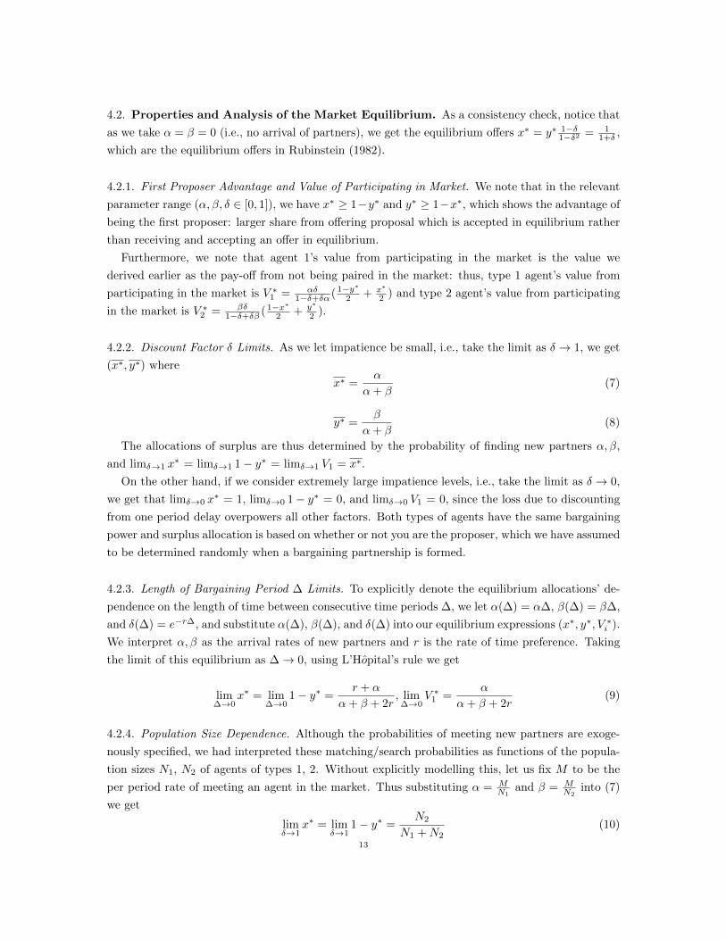
4.2. Properties and Analysis of the Market Equilibrium. As a consistency check, notice that

as we take α = β = 0 (i.e., no arrival of partners), we get the equilibrium offers x∗ = y∗ 1−δ1−δ2 = 1

1+δ ,

which are the equilibrium offers in Rubinstein (1982).

4.2.1. First Proposer Advantage and Value of Participating in Market. We note that in the relevant

parameter range (α, β, δ ∈ [0, 1]), we have x∗ ≥ 1−y∗ and y∗ ≥ 1−x∗, which shows the advantage of

being the first proposer: larger share from offering proposal which is accepted in equilibrium rather

than receiving and accepting an offer in equilibrium.

Furthermore, we note that agent 1’s value from participating in the market is the value we

derived earlier as the pay-off from not being paired in the market: thus, type 1 agent’s value from

participating in the market is V ∗1 = αδ1−δ+δα ( 1−y∗

2 + x∗

2 ) and type 2 agent’s value from participating

in the market is V ∗2 = βδ1−δ+δβ ( 1−x∗

2 + y∗

2 ).

4.2.2. Discount Factor δ Limits. As we let impatience be small, i.e., take the limit as δ → 1, we get

(x∗, y∗) where

x∗ =α

α+ β(7)

y∗ =β

α+ β(8)

The allocations of surplus are thus determined by the probability of finding new partners α, β,

and limδ→1 x∗ = limδ→1 1− y∗ = limδ→1 V1 = x∗.

On the other hand, if we consider extremely large impatience levels, i.e., take the limit as δ → 0,

we get that limδ→0 x∗ = 1, limδ→0 1− y∗ = 0, and limδ→0 V1 = 0, since the loss due to discounting

from one period delay overpowers all other factors. Both types of agents have the same bargaining

power and surplus allocation is based on whether or not you are the proposer, which we have assumed

to be determined randomly when a bargaining partnership is formed.

4.2.3. Length of Bargaining Period ∆ Limits. To explicitly denote the equilibrium allocations’ de-

pendence on the length of time between consecutive time periods ∆, we let α(∆) = α∆, β(∆) = β∆,

and δ(∆) = e−r∆, and substitute α(∆), β(∆), and δ(∆) into our equilibrium expressions (x∗, y∗, V ∗i ).

We interpret α, β as the arrival rates of new partners and r is the rate of time preference. Taking

the limit of this equilibrium as ∆→ 0, using L’Hopital’s rule we get

lim∆→0

x∗ = lim∆→0

1− y∗ =r + α

α+ β + 2r, lim∆→0

V ∗1 =α

α+ β + 2r(9)

4.2.4. Population Size Dependence. Although the probabilities of meeting new partners are exoge-

nously specified, we had interpreted these matching/search probabilities as functions of the popula-

tion sizes N1, N2 of agents of types 1, 2. Without explicitly modelling this, let us fix M to be the

per period rate of meeting an agent in the market. Thus substituting α = MN1

and β = MN2

into (7)

we get

limδ→1

x∗ = limδ→1

1− y∗ =N2

N1 +N2(10)

13

while substituting into (9) we get

lim∆→0

x∗ = lim∆→0

1− y∗ =rN1N2/M +N2

2rN1N2/M +N1 +N2(11)

Thus, we see that the side with the smaller population in the market gets more, but not all, of

the surplus from bargaining. This result coincides with general intuition that the agent who can

more easily find new matches must be compensated more.

5. Hybrid Model Without Irrational Types

Let us take the model from section 3 and set q1 = q2 = 0, so that there are only rational

types in the model. Furthermore, we now look at the continuous time version of the model above,

where agents of type 1, 2 find new partners governed by a poisson process, where the arrival of

new opponent is exponentially distributed with parameters λ1, λ2, and corresponding cumulative

distribution functions G1, G2. This is a natural continuous-time generalization of our discrete model

consisting of Bernoulli trials of finding a new partner every period: which converges to Poisson

process of arrivals as we take limits,5 while the distribution of inter-arrival times of a Poisson Process

is exponentially distributed. Thus, there is a direct correspondence between parameters α, β and

λ1, λ2. Furthermore, discounting is now continuous: agents 1, 2 have instantaneous time preference

of r1, r2. We again simplify for notational convenience, r1 = r2 = r. Finally, we consider a hybrid

model (as in Abreu and Pearce (2007)) where agents engage in alternating offer bargaining game

if they do not find new partners, where they make alternating offers with discrete time interval ∆

between offers. However, the offers can be accepted at any time t in the time interval ∆ over which

the offer remains on the table.

This hybrid set up of discrete time alternating offering with continuous time offer acceptance is

assumed as a way to maintain Rubinstein bargaining structure (which relies on alternating offers)

but also use war of attrition style acceptance action spaces. This incorporates an optimal stopping

element in bargaining, which will be useful when we consider reputation building with behavioral

types. Rubinstein bargaining model doesn’t sit well in continuous time, since the alternating offer

structure is lost in the limit; thus we consider this hybrid model to approximate and get around this

concern. With this hybrid set up, we are able to use a war of attrition style analysis without running

into well-known problems of defining strategies and outcomes in continuous time; thus bypassing

concerns of “openness” faced when modelling with continuous-time extensive games.

5.1. The Market Equilibrium. In equilibrium, we will get efficiency, since there is no uncertainty

(no irrational types). Furthermore, since all parameters are the same across all agents of the same

type, we can impose symmetric strategy subgame perfect Nash equilibrium, where all of agents of

types 1,2 use the same strategy. Finally, due to the stationary structure of the environment, we can

impose stationarity of strategies. Thus, we look for a market equilibrium similar to the one derived

in the discrete time model.

5Recall that binomial distribution with parameters n and pn converges to the Poisson distribution with parameter r,

when npn → r, as n→∞.

14

Let us define x, y as the stationary offers which agent 1 offers 2 and 2 offers 1 on the equilibrium

path. Then, these offers must be such that they make the opponent indifferent between accepting

immediately when the offer that is made, and waiting for time ∆. We note that if player i is in

the period lasting time ∆, where j has made him an offer; if i is going to accept j’s offer, it is a

dominant action for him to accept this offer immediately after the offer is made.

Thus, these offers x, y should satisfy:6

1− y = xe−(λ2−λ1)∆e−r∆ (12)

+1− y + x

2(1− e−λ1∆)e

−r(

1−e−λ1∆∗(λ1∆+1)

λ1(1−e−λ1∆)

)+

1− y + x

2e−λ1∆e−r(∆+1/λ1)(1− e−λ2∆)

1− x = ye−(λ1−λ2)∆e−r∆ (13)

+1− x+ y

2(1− e−λ2∆)e

−r(

1−e−λ2∆(λ2∆+1)

λ2(1−e−λ2∆)

)+

1− x+ y

2e−λ2∆e−r(∆+1/λ2)(1− e−λ1∆)

These are player i’s indifference conditions (for i = 1, 2 respectively) between accepting j’s offer

immediately and waiting for ∆ time, for j 6= i:

• The first term is the case where neither agent gets new partner in time ∆.

• The second term is the case where player i gets new partner within time interval ∆, in

which case with probability 1/2 he is proposer and with probability 1/2 he is receiver due

to random draw of 1st mover.

• The third term is the case where player j gets new partner within time interval ∆ and

player i gets an arrival after time ∆. By the memorylessness property of the exponential

distribution, player i gets a new partner in ∆ + 1/λi units of time in expectation.

Solving the system for (x, y) gives us the stationary market equilibrium values (x, y) satisfying

market equilibrium strategies (f , g) for agents of type 1 and 2, where:7

f(ht) =

1− x if ht ∈ Ht

o1,

A if ht ∈ Htr1 and last offer 1− y ≥ 1− y∗

R otherwise

6In deriving this equilibrium, we use the following facts: For X ∼ Expon (λ1),Y ∼ Expon (λ2), X ⊥⊥ Y . E(X) = 1/λ1,

Pr(X < Y ) = λ1λ1+λ2

.

Let us define E(X|X ≤ τ) = A. By memorylessness property of exponential distribution, E(X|X ≥ τ) = τ + 1/λ1.

Thus, by law of total expectation,

E(X) = 1/λ1 = (1− e−λ1τ )A+ e−λ1τ (τ + 1/λ1). Thus, A =1/λ1−e−λ1τ (τ+1/λ1)

1−e−λ1τ.

7This yields an efficient, symmetric SPNE, since there is no uncertainty. The explicit solutions for x, y can be explicitlyderived but are cumbersome formulas which do not provide much intuition. Thus, instead of including these formulas,

we derive and discuss limiting properties below and compare the results to our discrete model.

15

g(ht) =

1− y if ht ∈ Ht

o1,

A if ht ∈ Htr1 and last offer 1− x ≥ 1− x∗

R otherwise

5.2. Consistency in Limits. As a consistency check, comparing this hybrid model to our discrete

time analog, we note that

lim∆→0

x = lim∆→0

1− y =λ1 − λ1e

−rλ2 + r

λ1 + λ2 − λ2e−rλ1 + λ1e

−rλ2 + 2r

(14)

and

limr→0

x = limr→0

1− y =λ1

λ1 + λ2(15)

We conclude that our models are consistent, as in the limit as r → 0 (analog of δ → 0), we

see that the equilibrium allocations are determined by the relative size of the arrival rates of new

partners (analog of the arrival probabilities of new partners αα+β ).

6. Continuous-Time Model With Irrational Types

6.1. The Coase Conjecture. In the context of reputation-building bargaining, the Coase Conjec-

ture8 is valid if: when your opponent is known to be rational and believes that you are a behavioral

type with any positive probability, your opponent must give in right away to your possibly irra-

tional demand. There are two important consequences of the Coase Conjecture result being satis-

fied. Firstly, it is necessary in an equilibrium where rational types mimic the irrational demands of

behavioral agents. Secondly, it reduces the set of actions of each player at each time to a 2-action

space: either continue mimicking irrational type’s demand or accept your opponent’s irrational de-

mand. Thus, the 2-action space makes intermediate offers irrelevant and reduces the problem to an

optimal stopping, war of attrition game.9

We provide a condition, which we call the “Coase Conjecture condition,” such that if the condition

is satisfied, the Coase Conjecture is valid. The Coase Conjecture condition compares the pay-off to

rational player i from accepting the opponent’s irrational demand of 1 − θj to the most profitable

alternative action. In Abreu and Gul (2000), the bargaining partnership is bilateral and there is no

outside option (i.e., outside option pay-off is 0), thus, the Coase Conjecture condition trivially holds:

1 − θj ≥ 0, for all possible irrational types θj ∈ ( 12 , 1]. Thus, they can always analyze reputation-

building by reducing the game to a continuous-time war of attrition. On the other hand, all results

in Compte and Jehiel (2002), where reputation cannot be built up, arise due to the underlying

assumption (a violation of the Coase Conjecture condition) that 1− θj ≥ vj , where vj is the player

j’s outside option pay-off. Thus, rather than accepting the irrational opponent’s demand, the agent

8See Gul, Sonnenschein, and Wilson (1986) for details.9To further explain the importance of this second implication, we recall that in the bargaining model, the offer

space [0, 1] is infinite; thus if the Coase Conjecture condition fails to hold, intermediate offers (those not including

your irrational demand or accepting your opponent’s irrational demand) might be candidate equilibrium strategiesto consider. However, with just the 2-action space, analysis of the game as a war of attrition greatly simplifies the

possible equilibrium strategy space.

16

is always better off taking his outside option. Consequently, it is never optimal for a rational agent

to try to build a reputation by mimicking irrational type’s demand.

In our paper, the Coase Conjecture condition

1− θj ≥ (e−rj/λj ) ∗ Vj (16)

compares the pay-off of accepting the opponent’s irrational demand with the expected pay-off from

waiting for a new partner. The expected time for the arrival of a new partner is 1/λj and Vj is a

rational player j’s expected pay-off from meeting a new bargaining partner, which in our model is

endogenously determined in equilibrium (depending on prior probabilities of irrationality, irrational

type’s demands, discount rates, and arrival rate of new partners for both agents).

For reputation-building in bargaining models to be reduced to simple, continuous-time war of

attrition games—where rational players mimic the irrational demands of behavioral players and the

bargaining game turns into an optimal stopping problem—as in Abreu and Gul (2000), it is necessary

that the Coase Conjecture condition holds. We can think of more complex non-stationary war of

attrition games which do not necessarily need the Coase Conjecture condition to hold. However,

with a unique stationary irrational demand, θi,10 for each player i, we obtain only a simple war of

attrition bargaining game where, if the Coase Conjecture condition holds, there is possible reputation

build up, where rational agent i either mimics being an irrational type by demanding θi or concedes

by accepting his opponent’s irrational demand, 1− θj .

6.2. Introducing Irrational Types. We now allow for irrational types in the market: p, q ≥ 0.

Let us first assume that the Coase Conjecture condition holds and thus solve the continuous-time

war of attrition strategies: distribution functions F1, F2 over conceding times. Upon solving for these

potential equilibrium strategies F1, F2 (as in Abreu and Gul (2000)), we can then check under what

market environment the endogenous outside option (value from meeting new opponent) satisfies

the Coase Conjecture condition, thus, concluding, under what market conditions, equilibrium with

reputational build-up and delay are possible.

Let us consider agent type i’s problem. Let us denote by t ∈ [0,∞], the time after starting

bargaining with a new partner (i.e., t=0 is the time at which the agent is paired with a new partner).

Let us denote by Vi, the expected pay-off to a rational agent of type i from being matched with a

new partner.

10Extending the analysis to include irrational players following non-stationary strategies, such as in Abreu and Pearce

(2007) is possible, but beyond the scope of this paper.

17

A rational agent i’s utility from conceding at time t is

ui(t) = θiFj(0) +

t∫0

θie−rix(1−Gi(x))(1−Gj(x))dFj(x) (17)

+ (1− θj)e−rit(1−Gi(t))(1−Gj(t))(1− Fj(t))

+

t∫0

Vie−rix(1−Gj(x))(1− Fj(x))dGi(x)

+

t∫0

Vie−ri(x+1/λi)(1−Gi(x))(1− Fj(x))dGj(x)

We are trying to determine the equilibrium functions F1, F2.11 This will allow us to compute Vi

and check under what conditions the Coase Conjecture is satisfied, the war of attrition reduction of

the game is valid, reputation can be built up, and delay and inefficiency exist in equilibrium.

Maximizing the rational player i’s utility with respect to concession time t (i.e., the agent must

be indifferent between conceding at any time in the support of his mixed strategy distribution) gives

∂

∂tui(t) = θie

−t(ri+λi+λj)fj(t)− (1− θj)e−t(ri+λi+λj)fj(t) (18)

− (ri + λi + λj)(1− θj)e−t(ri+λi+λj)(1− Fj(t))

+ Vie−t(ri+λi+λj)λi(1− Fj(t))

+ Vie−t(ri+λi+λj)−ri/λiλj(1− Fj(t))

= 0

This gives us the first-order linear differential equation:

fj(t) + Fj(t)[(ri + λi + λj)(1− θj)− Vi(λi + λje

−ri/λi)]

(θi + θj − 1))︸ ︷︷ ︸ηj

(19)

=[(ri + λi + λj)(1− θj)− Vi(λi + λje

−ri/λi)]

(θi + θj − 1))︸ ︷︷ ︸ηj

Solving the differential equation by method of integrating factor shows that Fj is one of the family

of functions.

Fj(t) = 1− cje−ηjt (20)

Fi(t) is defined similarly by swapping subscripts. Now we need to solve for c1, c2 and η1, η2. Our

first condition comes from standard war of attrition arguments, also used in Abreu and Gul (2000),

that in equilibrium, both players cannot concede with discrete positive probability at time t = 0,

else it is strictly profitable for a player to deviate from this strategy, not concede at t = 0, and

11Recall that in models with rational and irrational types, in equilibrium, we need to only consider rational players’optimizing behavior, having specified irrational players’ actions. Thus, it suffices consider and maximize ui(t), a

rational player i’s utility.

18

wait for ε > 0 time before conceding. Thus, Fi(0) > 0 → Fj(0) = 0, thus we obtain one boundary

condition: (1− c1)(1− c2) = 0.

The other boundary condition arises from the claim proven in Abreu and Gul (2000); its analog can

be proven in our model. The probability of irrationality of both players must reach 1 simultaneously

at time we denote as τ < ∞. The intuition behind this claim is that if player i was rational and

knew that player j is irrational, then i would concede immediately (assuming the Coase Conjecture

condition is satisfied).

Thus by Bayes’ theorem:

1 = Pr(player i concedes by time τ | player i is rational) (21)

=Pr(player i concedes by time τ)

player i is rational

=Fi(τ)

1− ziThus,

Fi(τ) = 1− e−ηiτ = 1− zi (22)

To work out which player(s) have c = 1, we solve Fi(Ti) = 1 − e−ηiTi = 1 − zi, which implies

Ti = −ln(zi)ηi

. If T1 = T2, where we call both players 1 and 2 being ‘equally strong,’ then c1 = c2 = 1.

If Ti < Tj , where we call player i ‘strong’ and player j ‘weak,’ then ci = 1, cj < 1. The terminology

refers to how long it takes each player to build a reputation and convince his opponent of irrationality.

The ‘weak’ player, j, has to concede for a longer amount of time before convincing his opponent

of his irrationality (with probability 1). The ‘weak’ player thus concedes with discrete probability,

1− cj > 0, at time 0 to ensure that both players finish conceding at the same time τ = min{T1, T2}.There are three conditions that need to be satisfied for such delay an mimicking equilibrium to

exist: (1) η > 0, or equivalently, τ ≥ 0, (2) ci = 1→ cj ≤ 1, and (3) the Coase Conjecture condition.

6.2.1. Symmetric Case. Let us first consider the fully symmetric case with r1 = r2 = r, λ1 =

λ2 = λ, z1 = z2 = z, and θ1 = θ2 = θ ∈ ( 12 , 1]. We will thus look for symmetric mixed strategies,

where the cumulative distribution of concession time follows F1 = F2 = F . V1 = V2 = V is the

expected pay-off for a rational agent from finding a new partner.

In the symmetric case, both players are ‘equally strong’, T1 = T2 = τ , therefore c = 1.

F (t) =

1− e−ηt if t ≤ τ

1− z if t > τ(23)

Recall, that the function F (t) is not a cumulative distribution function: it is the ex ante prob-

ability that a player has conceded by time t, prior to knowing whether he himself is rational or

irrational.

If the player is irrational, he will never concede, so his cumulative distribution of concession

times is trivially 0 for all t. Let R(t) denote the cumulative distribution function of rational agent’s19

concession time. Then, by Bayes’ Rule we get normalization that:

R(t) =

1−e−ηt1−z if t ≤ τ

1 if t > τ(24)

Next, we compute V , a rational player’s expected pay-off from a new partner, using what we know

about the equilibrium strategy. We know that the support over which a rational type concedes is

t ∈ (0, τ ]. Since a rational agent plays a mixed strategy in equilibrium, where he mixes over

concession times in the support of F , by definition, he must be indifferent between conceding at any

time t in the support of F . Consider a rational player giving up at time ε > 0, where he gets pay-off

1− θ. As we take limε→0 e−rε(1− θ) = 1− θ. Thus,

V = 1− θ (25)

Thus, in the symmetric case, the Coase Conjecture condition is always satisfied, since 1 − θj ≥e−r/λ(1 − θj). Consequently, the game can always be reduced from a structured alternating offer

game to a continuous time war of attrition optimal stopping game, and a rational player will follow

the equilibrium strategy determined by the cumulative distribution over concession times R(t), where

R(t) =

1−e−ηt1−z , if t ≤ τ

1, if t > τ(26)

where τ = −ln(z)η ≥ 0 and η = r(1−θ)+λ(1−θ)(1−e−r/λ)

(2θ−1) > 0.12

It is worth noting that since e−r/λ ≤ 1, η ≥ ηag and τ ≤ τag, where subscript “ag” refers to

Abreu and Gul (2000). Thus, potential delay is reduced in a market setting with λ > 0.

From this simple, symmetric case, we can get intuition by evaluating how changing individual

parameters impact delay (and hence efficiency). In the equilibrium, τ measures the potential delay,

as it is the last time by which a rational player must concede. Since η > 0, ci = cj = 1, and Coase

Conjecture condition is always satisfied, such an equilibrium always exists. Over the next few pages,

we provide a series of diagrams and explanations which illustrate the impact on τ (potential delay),

in the symmetric case of our model as compared to Abreu and Gul (2000), when:

• Changing the rate of discounting: r

• Changing the irrational type’s demand: θ

• Changing the prior probability of irrationality: z

• Changing the rate of arrival of new partners: λ

12We check that our distribution is consistent with Abreu and Gul (2000), since when λ = 0 (i.e., no arrivals of newpartners) and αi = αj = θ (symmetric case),

Fi,ag(t) = Fj,ag(t) = FAG(t) =

1− e−r(1−θ)

2θ−1t

= 1− e−ηagt, if t ≤ τag1− z, if t > τag

(27)

as in Abreu and Gul (2000), since with λ = 0, η = ηag . Also, V (z = 0) = 1 − θ = Vag in the symmetric case. Note

that “ag” refers to Abreu and Gul (2000).

20

• As impatience or rate of discounting, r, increases, potential delay, τ , decreases. This is an

intuitive result: the more impatient a player is, the higher his opportunity cost from delaying

is, i.e., higher cost of mimicking irrationality and not having opponent concede. Thus, the

more impatient players are, the less delay in reaching agreement. In the extreme case, as

r →∞, τ → 0.

Figure 2. Numerical simulation of the effect on τ from changing r in the symmetric case.

21

• As the irrational type’s demand, θ, increases, potential delay, τ , increases. The more extreme

irrational types make their demands, the less attractive the pay-off 1 − θ is relative to θ.

Therefore, the gain from convincing an opponent of one’s irrationality is high, and thus

rational players are willing to mimic irrational types for longer in the hopes that their

opponent will concede. Thus, η decreases (slower concession) in response to an increase in

θ, and thus, for fixed z, τ is higher. Consequently, there is more potential delay.

Figure 3. Numerical simulation of the effect on τ from changing θ in the symmetric case.

22

• As the proportion of irrational types in the population, z, increases, potential delay, τ ,

decreases. Upon meeting a new partner, z is the prior belief of an agent that his opponent

is irrational. If this prior is high, it naturally takes less time to convince one’s partner of

being an irrational type. Thus, potential delay decreases.

Figure 4. Numerical simulation of the effect on τ from changing z in the symmetric case.

23

• As the arrival rate of new partners, λ, increases, potential delay, τ , decreases asymptotically

to a non-zero level, τag/2. Although in the symmetric case, V = 1− θ from all new partners

and there is no gain from a new partner from time t = 0 concession (i.e., c1 = c2 = 1),

reputation needs to be built up starting from the prior every time a new partner is found, as

previous partnership histories are private information. Thus, concessions must be made at

a faster rate (increase in η) to compensate for increases in the arrival rate of new partners.

As λ → ∞, τ → −ln(z)(2θ−1)2r(1−θ) = τag/2. τ ’s limiting level corresponds to half the potential

delay in Abreu and Gul (2000), which we denote by τag/2, because as λ → ∞, an agent is

without a partner half of the time.

Figure 5. Numerical simulation of the effect on τ from changing λ in the symmetric case.

24

6.2.2. Non-Symmetric Cases. We use the equilibrium properties we know to derive conditions

which must be satisfied for there to possibly be an equilibrium with reputational build-up, similar

to what we have thus far analyzed. From the boundary conditions, we know that in equilibrium,

Fi(τ) = 1− cie−ηiτ = 1− zi, thus

ci = zieηiτ = zie

ηi min{−ln(z1)η1

,−ln(z2)η2

} (28)

Furthermore, we can find the generic expression for Vi. A rational player i concedes at time ε > 0

as ε → 0 and thus is always guaranteed at least 1 − θj . However, if his opponent is the “weaker”

player, he may also get θi − (1 − θj) additional pay-off at time zero with probability Rj(0), where

Rj(t) =Fj(t)1−zj , is a rational player j’s mixed strategy cumulative distribution function. Thus, the

expected pay-off from a new partner is

Vi = zj(1− θj) + (1− zj)[(1− θj) + (θi − (1− θj))R2(0)] (29)

= (1− θj) + (θi − (1− θj))Fj(0)

= (1− θj)cj + θi(1− cj)

Now, given the parameters of the model, we can check whether there are equilibria which satisfy

the following: either c1 = 1 and c2 ≤ 1, and/or c2 = 1 and c1 ≤ 1. We can hypothesize each of

these cases, ci = 1 for i = 1, 2 and check whether there exists cj ≤ 1. Given our hypothesis that say

ci = 1,

cj = zjeηjτ (30)

= zjemin{−ln(zi)

ηi,−ln(zj)

ηj}

=zj

zηj/ηii

Then, we calculate Vi and Vj to make sure that the Coase Conjecture condition is satisfied.

Note that for the ‘weak’ player j (with cj < 1), Vj = 1 − θi always satisfies the Coase Conjecture

condition.13 Thus, we want to check whether Vi, the rational ‘strong’ player i’s expected pay-off

from a new partner, satisfies the Coase Conjecture condition. The intuition behind this is that the

‘strong’ player (with ci = 1) gets a favourable ‘gift’ (receiving θi > 1− θj) with discrete probability

Fj(0) > 0 from a new ‘weak’ bargaining partner conceding at time 0. Even when the ‘strong’ player

knows with probability 1 that his opponent is of the irrational type, if this ‘gift’ is very profitable

and the arrival rate of new partners is high enough, then the ‘strong’ player may prefer to wait for

an arrival instead of yielding to irrational opponent (contradicting the Coase Conjecture condition).

As rudimentary comparative statics, we look at how each of our model’s parameters — discount

rates, proportion of irrational types, arrival rates of new partners, and irrational demands—affect

surplus allocation by skewing the individual parameter while keeping everything else symmetric

between the two sides.

13In this case, 1− θi ≥ e−rj/λj (1− θi), thus the Coase Conjecture condition holds trivially for the ‘weak’ player.

25

• Different Discount Rates:

The relative impatience of the two sides (incorporated by the discount rates) is one of the

fundamental determinants of bargaining power in our model. Just as in Rubinstein (1982),

the more impatient side has less bargaining power and gets a smaller expected pay-off in

equilibrium, all other characteristics kept symmetric between the two sides. In our model,

a ‘weak’ agent 2 (r2 ≥ r1) concedes with discrete probability at time 0 (c2 ≤ 1) and thus

gets pay-off 1 − θ1, while a ‘strong’ agent 1 benefits from being conceded to with discrete

probability at time 0 and gets expected pay-off V1. We note that the potential delay (τ)

decreases as one side gets increasingly impatient, as deals are agreed upon faster. We see

that if one side is too impatient, i.e., r2 > r∗2 , the Coase Conjecture condition is violated,

and such a mixed-strategy mimicking equilibrium which we focus on doesn’t exist.

Figure 6. Numerical simulation of the effect on τ and e−r1/λ1V1 from increasing r2,thus making agent 2 more impatient, while leaving all other parameters symmetricamongst the two types of agents.

26

• Different Proportions of Irrational Types:

Other characteristics kept symmetric between the two sides, if agent 2 starts off believing

that his bargaining partner, agent 1, is irrational with higher probability (z1 ≥ z2), a higher

prior, it takes agent 1 a shorter time to build a reputation, thus τ decreases and a ‘strong’

agent 1 gets a ‘gift’ from a ‘weak’ agent 2 conceding with discrete probability at time zero.

If agent 2’s prior of agent 1’s irrationality is too high, i.e., z1 > z∗1 , the Coase Conjecture

condition is violated, and such a mixed-strategy mimicking equilibrium which we focus on

doesn’t exist.

Figure 7. Numerical simulation of the effect on τ and e−r1/λ1V1 from increasingz1, agent 1’s prior probability of irrationality, while leaving all other parameterssymmetric amongst the two types of agents.

27

• Different Arrival Rates of New Partners:

Other characteristics kept symmetric between the two sides, if agent 1 can find new

partners more frequently than agent 2 (λ1 ≥ λ2), his endogenously determined outside option

is more valuable and can credibly be used as a threat by agent 1 to increase his bargaining

power. As λ1 increases, potential delay (τ) decreases, ‘strong’ agent 1’s bargaining power

increases, and ‘weak’ agent 2’s bargaining power decreases as he has to concede with larger

discrete probability at time 0. If the arrival rates are too skewed in favor of agent 1, i.e.,

λ1 > λ∗1, then such a mixed strategy mimicking equilibrium which we focus on doesn’t exist,

as agent 1’s bargaining power becomes too large and the Coase Conjecture condition is

violated.

Figure 8. Numerical simulation of the effect on τ and e−r1/λ1V1 from increasingλ1, arrival rate of new partners for agent 1, while leaving all other parameterssymmetric amongst the two types of agents.

28

• Different Irrational Demands:

Other characteristics kept symmetric between the two sides, we note that ηi and ηj are

not monotonic for all ranges of θi and θj . As in Abreu and Gul (2000), the side with the

lower irrational demand is ‘strong.’ However, the pay-off impact of differences in θi and θj

are highly dependent on the other parameters (z, λ, r) for i, j. In our numerical example,

for the defined parameter space, note that such a mixed strategy mimicking equilibrium

only holds in the range θ1 ∈ [.51, .7], i.e., θ1 < θ2, in figure 9. Given the parameter space,

θ∗∗1 ≈ .5617 yields a rational player 1 the highest expected pay-off from a new partner. Note

that τ monotonically increases in response to changes in θ1.

Figure 9. Numerical simulation of the effect on τ and e−r1/λ1V1 from increasingθ1, irrational demand for agent 1, while leaving all other parameters symmetricamongst the two types of agents.

29

6.3. Equilibrium when the Coase Conjecture Condition is Violated. If the Coase Conjec-

ture condition is violated, 1− θj < e−ri/λiVi, in our model, it is violated only for the ‘strong’ player

(as it trivially holds for the ‘weak’ player). Thus, a rational ‘strong’ player would never accept his

‘weak’ opponent’s irrational demand in equilibrium (since he prefers not to accept it even when he

believes with probability 1 that his ‘weak’ opponent is irrational) since his endogenous outside op-

tion of waiting for a new bargaining partner is more profitable. Therefore, in equilibrium, a rational

‘strong’ player will mimic the irrational type and a rational ‘weak’ player will prefer to concede as

early as possible, i.e., at time 0, by accepting his ‘strong’ opponent’s irrational demand (‘one-sided

reputation’).

We note that this equilibrium is distinct from the equilibrium derived in Compte and Jehiel (2002),

who consider a model where both players’ exogenous outside options violate the Coase Conjecture

condition. In our model, if the Coase Conjecture condition is satisfied, both sides mimic irrationality.

However, if the Coase Conjecture condition is violated, the ‘strong’ player mimics and the rational

‘weak’ player immediately concedes to the strong player.

7. Revisiting Applications

Our model elaborates on the relationship between supply and demand which is fundamental to

the study of economics. The model explains how factors such as impatience, irrational demands,

and competition affect each side’s bargaining power in a market. It is the relative bargaining power

that determines the allocation of surplus from the transaction, whether it is the size of venture

capitalist’s stake in a company, wage given to the worker by the employer, collateral and haircuts

the borrower must give to the lender in a repo transaction, or the prices of assets in decentralized

markets for commodities, real estate, derivatives, or exotic securities (such as MBSs, CDOs, CDSs).

It is hard to empirically test the impact of bargaining delay and whether irrational mimicking-driven

bargaining causes this delay. However, the impact of relative bargaining power on the allocation of

surplus (i.e., wage negotiated by workers and price of asset agreed to by counter-parties) and how

this allocation changes in response to a change in the market environment can be assessed using

available data.

We should note that prices of assets are not the most ideal data with which to test the allocation

of surplus since our model abstracts from addressing more complex issues such as fundamental values

of assets. Our model best fits the framework of venture capitalist’s equity stake, since 100% of stake

is easily normalized to 1 unit surplus, and bargaining over how much of the stake is allocated to

the start-up manager compared to the venture capitalist (VC) is a clear division of the unit surplus.

Nevertheless, data on the VC stake is not readily available, while data on wages, prices of assets,

spreads on interest rates,... is available and has been analyzed in the empirical literature, so we tend

to focus on the impact of relative bargaining power on prices when describing empirical applications

of our model.

Finally, it is important to realize that our model is a highly simplified and stylized version of the

applications we hope to contextualize. The main simplifications are that each individual buyer is

identical and each individual seller is identical, and that each transaction generates a total surplus

of 1 (i.e., each worker produces the same output and each asset traded is identical). Decentralized30

markets are generally decentralized, because these characteristics are heterogeneous: over-the-counter

derivatives are highly idiosyncratic and each worker has different qualifications. Thus, these markets

differ from centralized markets such as stock markets, where each share of stock is identical to every

other share of stock for a particular firm. These idiosyncratic differences between each of the buyers

and each of the sellers might also lead to different surpluses from trade for different pairs (i.e., a

highly qualified worker with 20 years of work experience might be more productive and produce

more output for a firm than a worker who has little prior experience). Nevertheless, our model can

provide the framework to obtain key intuition for understanding important market events such as

unemployment, fire-sales, demand crunches, and liquidity crises.

7.1. Labor Markets & Wage Negotiations. Search theory is widely used in modelling labor

markets to describe the interactions between workers who seek employment and firms which have

vacancies to fill. In most cases, labor markets are highly decentralized where search frictions and

delay from labor strikes are widespread. It is important to understand that labor frictions arising

from delay in bargaining, strikes, unemployed workers, and excess capacity all adversely affect pro-

duction and output of the real economy. Although wage bargaining and labor negotiation data (such

as offers, counter-offers, demands, and delay) is hard to find, we attempt to explain certain events

in the labor market.14

Let us call type 1 agents “firms” and type 2 agents “workers.” During recessions, aggregate

demand dries up in the economy; thus, production falls, firms start downsizing, increase lay-offs,

and decrease hiring (λ2 decreases). On the flip side, unemployed workers searching jobs increases

(λ1 increases). We note that λ2 changes can also encapsulate frictions arising from displaced workers

and misaligned skill-set due to a structural shifts (all factors which have been raised in explaining

the recent increase in unemployment).15 The Beveridge Curve exhibits this very relationship of

vacancy rates and unemployment rates being negatively correlated (see figure 10), suggesting that

our interpretation of λ1 and λ2 moving in opposite directions during booms and busts holds in

the data.16 Furthermore, impatience levels of unemployed workers having a hard time finding jobs

increases (r2 increases), while firms who cut production in response to an aggregate demand dry-up

become less impatient (r1 decreases). Not only are firms more likely to be irrational (z1 increases)

and ask for higher surplus, lower wages (θ1 increases); but workers also do not appreciate nominal

wage cuts to begin with, thus, θ2 may remain unchanged. Thus, during business cycle downturns

and recessions, labor loses bargaining power, wages decline, search frictions increase, and delay in

reaching agreement (which can be loosely proxied by duration of unemployment) increases. In the

data, we point out how unemployment and wages are negatively correlated (see figure 11), and how

during recessions, duration of unemployment increases (see figure 12).

Our model can help contextualize an interesting debate which arose in the aftermath of the

crisis in response to the American Recovery and Reinvestment Act of 2009 (colloquially known as

14Literature on search models in labor markets includes Phelps (1970), Blanchard and Diamond (1990, 1991),Mortensen (1986), Rogerson, Shimer, and Wright (2004), Mortensen and Pissarides (1999), and Pissarides (1988).15Recent literature involving labor market adjustments due to long-term unemployment and displaced workers includes

Arulampalam, Gregg, and Gregory (2001), Jacobson, LaLonde, and Sullivan (2003), and Couch and Placzek (2010).16For literature regarding the Beveridge Curve refer to Blanchard and Diamond (1990).

31

Figure 10. The graph shows the negative correlation between unemployment rateand vacancy rate (the Beveridge Curve) decomposed into the time-series of thetwo rates. This relationship seems to suggest that our interpretation of λ1 and λ2

moving in opposite directions during booms and busts holds in the data.Data source: Federal Reserve Economic Data, Federal Reserve Bank of St. Louis

the “stimulus”). Particularly, the subject of contention was the extension of the social safety net

for unemployed workers promised by the stimulus: expanding the food stamp program, increasing

unemployment insurance, increasing worker tax cuts, and extending other unemployment benefits

comprised $296 billion of the $840 billion stimulus package.17 The debate was over how these welfare

programs would affect the underlying incentives of unemployed workers (i.e., how r and θ change as

a response to the stimulus program).

Economists such as Robert Barro,18 believed that these programs provided disincentives to un-

employed workers to not actively search for jobs and instead free-ride on government support. This

outlook suggests that as a result of the stimulus, workers are more patient despite being unemployed,

due to increased unemployment benefits (r2 decreases). Also, workers are less likely to participate

vigorously in the job market due to the unemployment benefits providing disincentives (λ1 decreases).

Thus, delay increases: loosely proxied by an increase in duration of unemployment. Furthermore,

θ2 also increases as the unemployment benefits have increased the ‘perks’ of staying unemployed,

thus workers are less motivated to look for low-paying jobs, demand high wages, and resist nominal

wage cuts relative to previous employment. On the other side of the debate, economists such as Paul

Krugman,19 advocated that these programs work, do not disincentivize workers, but rather provide

17Figures reported from Executive Office of the President of the United States (2014).18Barro (2011).19Krugman (2009).

32

Figure 11. The graph shows the negative correlation between unemployment rateand wages: our model suggests that this result is partly due to workers losingbargaining power during economic slumps.Data source: Federal Reserve Economic Data, Federal Reserve Bank of St. Louis

a safety net which takes care of basic needs and allow workers to more actively search for jobs (λ1

increases), and impatience (r2) and nominal rigidities (θ2) remain unchanged. These economists

argue that the welfare program decreased delay (i.e., long term unemployment) and helped mitigate

the impact of the Great Recession on the labor market and unemployment.20

Accessing the validity of either side of this argument is beyond the scope of this paper, but we

simply depict how different theories fit into our model and which parameter shifts explain each side

of the argument: a mere depiction of an application of our model.

7.2. OTC Asset Markets: Fire-sales, Demand Squeezes, and Panics. Let us consider de-

centralized, over-the-counter asset markets, such as markets for commodities, derivative securities,

collateralized debt obligations, mortgage-backed securities, credit default swaps, and exotic financial

securities. These markets do not have central exchanges, such as the stock exchange, thus, there

are search frictions: buyers and sellers in the market must individually search for counter-parties

and engage in bilateral bargaining over terms of trade. Our model can help explain the phenomena

of panics and resulting fire-sales from a microeconomic perspective. While papers such as Kiyotaki

and Moore (1995) explain how systemic panics spread via credit channels and fire-sales, our model

hopes to take one step back and explain how market environment might change during the lead

up to the panic: what changes in characteristics of market participants cause skewed allocation of

20We note that our model ignores important factors such as changes in aggregate demand, which Krugman would

consider of first order of importance when evaluating the success of such policies.

33

Figure 12. The graph shows how during recessions (shaded regions on the graph),duration of unemployment—which we use as an imperfect proxy for delay in reachingagreement in our model—increases.Data source: Federal Reserve Economic Data, Federal Reserve Bank of St. Louis

surplus from trade. We attempt to explain how and why assets are sold at fire-sale prices to begin

with by looking at bilateral bargaining partnerships of individual agents in the market.21

Let us call type 1 agents the “buyers” and type 2 agents the “sellers” of the asset. For example,

consider the market for mortgage-backed securities. We abstract from the so-called “fundamental

valuation” of the asset and consider the price of the asset to reflect market confidence and be

determined by the relative bargaining power of buyers and sellers. Up until the start of the Great

Recession in 2007-8, prices of MBSs were stable and the market was functioning well. The Great

Recession reflected a sudden loss of confidence in these exotic financial products. Supply of these

products had slowly increased in the market during normal times, thus λ1 was large: population

of sellers was large thus buyers could more frequently meet new counter-parties to bargain/trade

with. However, after the loss of confidence in MBSs, the population of buyers in the market fell

dramatically, thus λ2 fell: sellers couldn’t find counter-parties. Furthermore, due to the run for

liquidity (during periods of crisis, risk aversion increases and demand for liquidity rises), supply

of MBSs on the market ballooned, thus λ1 increased even further. Furthermore, lenders who lent

to buyers on a short-term basis demanded cash and more liquid collateral, thus, these financial

institutions wanted to sell and liquidate their MBS holdings, r2 increased: sellers became increasingly

impatient to sell their assets. Finally, buyers losing confidence in MBS would increase z1 and θ1:

buyers are more likely to act irrationally and ask for even higher surplus (lower prices). We see that

21Other literature on search frictions and OTC markets includes Lagos, Rocheteau, and Weill (2011), Lagos and

Rocheteau (2007, 2009), Bernardo and Welch (2004), Dufe, Grleanu, and Pedersen (2005), and Weill (2007).

34

all of these changes caused bargaining power of buyers to increase while that of sellers to decrease.

Thus, allocation of surplus shifts in favor of buyers during recessions, explaining the collapse of asset

prices in the market.

7.3. Repo Market: Runs and Credit Squeezes. In an earlier section we depicted the application

of our model to demand squeezes in asset markets. In a similar vein, we use our model to attempt

to provide intuition for credit squeezes, such as the one witnessed by the financial sector during the

Great Recession.

High leverage and increased reliance on short-term borrowing in the repo market were two phe-

nomena which were characteristic of the recent financial boom and bust leading to the Great Reces-

sion. Interbank borrowing on the repo market became increasingly prevalent in the run-up to the

crisis and when lenders lost confidence in the liquidity and solvency of their counter-parties, demands

for collateral were tightened and haircuts were increased.22 Our model abstracts from addressing the

underlying questions of insolvency, illiquidity, and how a crisis of confidence arises; however, we can

provide intuition regarding the allocation of surplus from transactions and the relative bargaining

power in instances of liquidity panics.23

Let us call type 1 agents “borrowers” and type 2 agents ”lenders” in the repo market. When banks

and shadow banks who were borrowers faced a run on wholesale funding, as lenders lost confidence

in the borrower’s ability to remain solvent and repay the debt obligations, the market environment

changed. Many lenders left the market due to fear while banks reliant on repo borrowing (either

insolvent or illiquid) increased in the market (recall Lehman Brothers and Bear Stearns), thus λ1

decreased while λ2 increased. Fearing contagion and liquidity crisis leading to a retail banking

panic on deposits, these systematically important institutions faced incredibly short time deadlines

in which they had to secure funding and prevent bankruptcy. Thus impatience on the part of

borrowers r1 became extremely high. Finally, due to the loss of confidence amongst lenders, z2

and θ2 increased as lenders started to demand greater quantities of safer collateral such as cash

and Treasury bills, rather than MBSs and CDOs which were facing runs and fire-sales as explained

above. Thus, bargaining power was highly skewed towards the lenders in the repo market and

financial institutions such as Lehman Brothers and Bear Stearns, which had grown highly dependent

on short term repo borrowing, faced turmoil. Their assets lost value due to a widespread loss of

confidence in asset-backed securities such as CDOs and MBSs, their borrowing costs increased as

collateral demands tightened and haircuts increased,24 and they tried to liquidate exotic assets on

22Gorton and Metrick (2009).23Literature on credit squeezes and bank runs includes the seminal paper Diamond and Dybvig (1983), and empiricalpapers on the recent repo market run include Gorton and Metrick (2009), Gorton (2007), and Hordahl and King

(2008).24A loss of confidence in shadow banking is reflected in credit default swap spreads for AIG, Lehman, and Merrill

Lynch. Figure 4 on page 19 of Brunnermeier (2008).

35

the market at fire-sale prices to both decrease leverage, prevent run on the bank, and put up safe

collateral.25

In short, from our model, we get an intuitive micro-bargaining perspective on how credit con-

straints and fire-sales26 became an issue for highly leveraged financial institutions whose balance

sheets were loaded with exotic, risky assets often times backed by sub-prime debt, during the Great

Recession. We explain the bilateral bargaining underpinnings of collateral runs and flight to safety.

Figure 13. The graph, figure 2 on page 9 from Gorton and Metrick (2009), showshow during the Great Recession, haircuts on sub-prime structured products faceda run. Haircuts reaching 100% implies that sub-prime structured products were nolonger accepted as collateral. This shows the need for fire-sales of sub-prime backedstructured products (we modelled in section 7.2) and the loss of bargaining powerfor repo borrowers.

7.4. Venture Capital Markets. Our model fits the interaction between venture capitalists and

start-up managers extremely well, because, essentially, there is a clear unit pie (100% equity owner-

ship of the start-up) which the start-up and venture capitalist bargain over in exchange for capital

investment in the company. This measure of splitting a unit pie of surplus via buying equity stake

in the company is a better analog for our model than prices of assets or labor as analyzed above.

25Part IV, Chapter 18 of Financial Crisis Inquiry Report (2011) contains a detailed anecdotal account of the bargaining

between Lehman Brothers and its counter-parties JP Morgan, Citigroup, and Bank of America in the repo market,who increased their collateral demands, asking for more collateral and collateral in form of $5 billion in cash. The

account shows how J.P. Morgan and other counter-parties behaved like or mimicked irrational agents, by not willing

to accept riskier collateral and smaller haircuts.26Features fundamental to Kiyotaki and Moore (1995).

36

However, this data is not readily available and the empirical literature on venture capital market

doesn’t focus on equity stake allocation.27

Furthermore, it is a market where supply and demand feed off each other: for example, venture

capital firms mushroomed in the late 1990s along with technology start-ups during the Dot-com

bubble. Thus, it seems that this market is rarely highly asymmetric in participation of start-ups

and venture capitalists. We could draw a broad comparison to simultaneous supply and demand

increases during the Dot-com bubble as both λs increase. As a loose approximation, we do note

that in the symmetric case of our model, potential delay decreases as λ increases, as seen in figure 5.

This might explain the unbelievable rise of VC-backed technology firms and IPOs during the height

of the Dot-com bubble.

8. Conclusion

We develop a search-and-bargain model to understand the role of reputation building in de-

centralized markets. We endogenize the outside option which is modelled by a stochastic process

determining the arrivals of new bargaining partners, i.e., the search friction in the decentralized

market. The market equilibrium (i.e., bargaining strategies and the resulting allocation of the unit

surplus agreed to by the two sides) depends on the market environment, which we parameterize by

the relative rates of impatience, arrival rates of new partners, prior probability of irrational types in

the market, and irrational demand.

First, we develop a discrete-time model without behavioral types, akin to Rubinstein and Wolinsky

(1985), but with alternating offers. We derive a stationary subgame perfect Nash equilibrium and

find that the equilibrium is dependent on the relative discount rates, the relative population sizes of

the two populations, and the length of time between offers. The side that is more patient and has

a smaller population (higher likelihood of finding new bargaining partners each period) has greater

bargaining power and thus is compensated with higher surplus in equilibrium.

Second, we build a hybrid model without behavioral types, similar to Abreu and Pearce (2007),

where alternating offers are made in discrete time but can be accepted in continuous time. This

continuous time generalization of our model, with Poisson arrivals of new bargaining partners, allows

us to maintain the Rubinstein bargaining structure of alternating offers with war of attrition style,

optimal stopping action space for accepting offers. We derive consistency in limits between the

discrete and hybrid models: as agents become infinitely patient, surplus allocations are determined

by the relative arrival rates of new partners. Since the exponentially distributed arrival rates of new

partners are fundamentally rooted in population sizes, we once again find that allocation of surplus

is determined by the element of competition arising from relative population size differences; the

more scarcely populated side reaping higher surplus in equilibrium.

Third, we construct a continuous-time model with irrational types, generalizing Abreu and Gul

(2000) to include the endogenized outside option of meeting new bargaining partners in the search

27Literature describing the venture capital industry, deal sizes, industry and sector-wise analysis, and other empirical

studies includes Gompers and Lerner (1999, 2004), and Hellman (1998). However, the data and empirical analyses

in these papers cannot be used to test our model in the VC market. We would ideally want data on equity stakebargained for by the venture capitalist and start-up founder, and analyze how this allocation changed over the years

in response to changes in number of VC firms and start-ups.

37

market. We formulate the Coase Conjecture condition, which if satisfied, ensures that if a rational

player, believing with any positive probability that his opponent is irrational, chooses to concede,

he will concede immediately to the opponent’s irrational demand. We show that when the Coase

Conjecture condition is satisfied, there is a mimicking equilibrium, where rational types mimic the

irrational demands and engage in a war of attrition style, optimal stopping game, resulting in

two-sided reputation building and potential delay in reaching agreement. In our model, the Coase

Conjecture condition fails if one side’s outside option (expected pay-off from meeting a new partner)

is too high, giving him very high bargaining power. In this case, there is one-sided reputation building

and no delay in reaching agreement. Rational players on the ‘strong’ side mimic irrationality, rational

players on the ‘weak’ side immediately concede to their opponents’ irrational demand, and irrational

players on the ‘weak’ side are not able to trade in the market due to incompatible demands.

In analyzing the effect of the market environment on the value of the endogenized outside option,

a player’s bargaining power, and the potential delay in reaching agreement, we first consider the

symmetric case, where the Coase Conjecture condition is trivially satisfied and a mimicking equi-

librium always exists. We find that potential delay in reaching agreement decreases with greater

impatience, more frequent arrivals of new partners, higher prior probability of irrationality, and

smaller irrational demands for both sides. As long as the arrival rate of new partners is positive, the

potential delay in our model is always smaller than the potential delay in Abreu and Gul (2000).

Second, we consider the asymmetric case, where we vary only one parameter between the two sides,

leaving all other parameters symmetric. The side which is more patient, has a higher prior proba-

bility of irrationality, and a higher rate of arrival of new partners has greater bargaining power and

higher equilibrium pay-off due to discrete probability concession at time zero by the ‘weak’ rational

opponent. The player with a lower irrational demand has more bargaining power; however, the

pay-off is not monotonic in changes in irrational demand. As these parameters become increasingly

asymmetric, heavily favoring the ‘strong’ side of the market by increasing the endogenized outside

pay-off, the Coase Conjecture condition is violated, and a one-sided reputation-building equilibrium

exists, where only the ‘strong’ side can mimic irrationality in equilibrium.

These derived comparative statics of our model allow us to get intuition for how major market

events such as unemployment increases during recessions, fire-sale of assets during busts, and repo

market credit crunch during liquidity panics are driven by the micro-founded market conditions

which skew the relative bargaining power between counter-parties in these decentralized, search

markets.

38

References

[1] Abreu, Dilip, and Faruk Gul. “Bargaining and reputation.” Econometrica 68.1 (2000): 85-117.

[2] Abreu, Dilip, and David Pearce. “Bargaining, reputation, and equilibrium selection in repeated games with

contracts.” Econometrica 75.3 (2007): 653-710.

[3] Arulampalam, Wiji, Paul Gregg, and Mary Gregory. “Unemployment scarring.” The Economic Journal 111.475

(2001): 577-584.

[4] Barro, Robert J. “Keynesian Economics vs. Regular Economics.” Wall Street Journal August 23 (2011).

[5] Bernardo, Antonio, and Ivo Welch. “Liquidity and financial market runs.” Quarterly Journal of Econonmics 119

(2004) 135158.

[6] Binmore, Kenneth G., and Maria J. Herrero. “Matching and bargaining in dynamic markets.” The Review of

Economic Studies 55.1 (1988): 17-31.

[7] Blanchard, Olivier Jean, and Peter A. Diamond. “The aggregate matching function.” National Bureau of Eco-

nomic Research No. w3175. (1991).

[8] Blanchard, Olivier J., and Peter A. Diamond. “The Beveridge Curve.” NBER Working Paper R1405 (1990).

[9] Brunnermeier, Markus K. “Deciphering the liquidity and credit crunch 2007-08.” National Bureau of Economic

Research No. w14612. (2008).

[10] Compte, Olivier, and Philippe Jehiel. “On the role of outside options in bargaining with obstinate parties.”

Econometrica 70.4 (2002): 1477-1517.

[11] Couch, Kenneth A., and Dana W. Placzek. “Earnings losses of displaced workers revisited.” The American

Economic Review (2010): 572-589.

[12] Diamond, Douglas W., and Philip H. Dybvig. “Bank runs, deposit insurance, and liquidity.” The Journal of

Political Economy(1983): 401-419.

[13] Duffie, Darrell, Nicolae Garleanu, and Lasse Heje Pedersen. “Over-the-Counter Markets.” Econometrica 73.6

(2005): 1815-1847.

[14] Executive Office of the President of the United States. “The Economic Impact of the American Recovery and

Reinvestment Act of 2009 Five Years Later.” Final Report to Congress. (2014).

[15] Federal Reserve Economic Data, Federal Reserve Bank of St. Louis Civilian Unemployment Rate, Average Mean

Duration of Unemployment, Average Hourly Earnings of Production and Non-supervisory Employees: Total

Private, and Seasonally Adjusted Job Openings Rate: Total Nonfarm; U.S. Department of Labor: Bureau of

Labor Statistics http://research.stlouisfed.org/fred2/series. Accessed March 19, 2014.

[16] Fudenberg, Drew, David K. Levine, and Jean Tirole. “Incomplete information bargaining with outside opportu-

nities.” The Quarterly Journal of Economics 102.1 (1987): 37-50.

[17] Gale, Douglas. “Bargaining and competition part I: Characterization.” Econometrica 54, (1986a): 785-806.

[18] Gale, Douglas. “Bargaining and competition part II: Existence.” Econometrica 54, (1986b): 807-818.

[19] Gale, Douglas. “Limit Theorems for Markets with Sequential Bargaining.” Journal of Economic Theory 43,

(1987): 20-54.

[20] Garman, Mark B. “Market Microstructure.” Journal of Financial Economics 3.3 (1976): 257-275.

[21] Gehrig, Thomas. “Intermediation in search markets.” Journal of Economics & Management Strategy 2.1 (1993):

97-120.

[22] Gompers, Paul, and Josh Lerner. “An analysis of compensation in the US venture capital partnership.” Journal

of Financial Economics 51.1 (1999): 3-44.

[23] Gompers, Paul Alan, and Joshua Lerner. “The venture capital cycle.” MIT press 2004.

[24] Gorton, Gary B. “Information, liquidity, and the (ongoing) panic of 2007.” National Bureau of Economic Research

No. w14649. (2009).

[25] Gorton, Gary B., and Andrew Metrick. “Haircuts.” National Bureau of Economic Research No. w15273. (2009).

[26] Gul, Faruk, Hugo Sonnenschein, and Robert Wilson. “Foundations of dynamic monopoly and the Coase conjec-

ture.” Journal of Economic Theory 39.1 (1986): 155-190.

39

[27] Hellmann, Thomas. “The allocation of control rights in venture capital contracts.” Rand Journal of Economics

29 (1998): 57-76.

[28] Hordahl, Peter, and Michael King. “Developments in repo markets during the financial turmoil.” BIS Quarterly

Review 37 (2008).

[29] Jacobson, Louis, Robert J. LaLonde, and Daniel Sullivan. “The impact of community college retraining on older

displaced workers: Should we teach old dogs new tricks?.” Industrial and Labor Relations Review (2005): 398-415.

[30] Kiyotaki, Nobuhiro, and John Moore. “Credit cycles.” National Bureau of Economic Research No. w5083. (1995).

[31] Krugman, Paul. “How did economists get it so wrong?.” New York Times 2.9 (2009).

[32] Lagos, Richardo, and Guillaume Rocheteau. “Liquidity in asset markets with search frictions.” Econometrica 77

(2009): 403426.

[33] Lagos, Ricardo, and Guillaume Rocheteau, “Search in assets markets: Market structure, liquidity and welfare.”

American Economic Review 97 (2007) 198202.

[34] Lagos, Ricardo, Guillaume Rocheteau, and Pierre-Olivier Weill. “Crises and liquidity in over-the-counter mar-

kets.” Journal of Economic Theory 146.6 (2011): 2169-2205.

[35] Lamoureux, Christopher G., and Charles R. Schnitzlein “When it’s not the only game in town: The effect of

bilateral search on the quality of a dealer market.” The Journal of Finance 52.2 (1997): 683-712.

[36] McLennan, Andrew, and Hugo Sonnenschein. “Sequential bargaining as a noncooperative foundation for Wal-

rasian equilibrium.” Econometrica (1991): 1395-1424.

[37] Mortensen, Dale T. “Job search and labor market analysis.” Handbook of labor economics 2 (1986): 849-919.

[38] Mortensen, Dale T., and Christopher A. Pissarides. “New developments in models of search in the labor market.”

Handbook of labor economics 3 (1999): 2567-2627.

[39] Myerson, Roger B. “Game theory: analysis of conflict.” Cambridge, Mass.: Harvard University Press, 1991. Print

[40] Osborne, Martin J., and Ariel Rubinstein. “Bargaining and markets.” San Diego: Academic Press, 1990. Print.

[41] Phelps, Edmund S. “Microeconomic foundations of employment and inflation theory” New York: Norton, 1970.

Print.

[42] Pissarides, Christopher A. “The search equilibrium approach to fluctuations in employment.” American Economic

Review 78.2 (1988): 363-68.

[43] Rogerson, Richard, Robert Shimer, and Randall Wright. “Search-theoretic models of the labor market-a survey.”

National Bureau of Economic Research No. w10655. (2004).

[44] Rubinstein, Ariel. “Perfect Equilibrium in a Bargaining Model.” Econometrica 54, (1982): 97-109.

[45] Rubinstein, Ariel, and Asher Wolinsky. “Equilibrium in a market with sequential bargaining.” Econometrica 53,

(1985): 1133-1150.

[46] Samuelson, Larry. “Disagreement in markets with matching and bargaining.” The Review of Economic Studies

59.1 (1992): 177-185.

[47] Weill, Pierre-Olivier. “Leaning against the wind.” The Review of Economic Studies 74.4 (2007) 1329-1354.

40

PLEDGE:

This paper represents my own work in accordance with University regulations.

Undergraduate, Economics Department, Princeton University

E-mail address: athakur@princeton.edu

41