Banshee: A Practical Constraint-Based AnalysisToolkit

John Kodumal1 and Alex Aiken2

1 EECS Department, University of California, Berkeley2 Computer Science Department, Stanford University

Abstract. We introduce Banshee, a toolkit for constructing constraint-based program analyses. Banshee’s novel features include a code genera-tor for creating customized constraint resolution engines, an incrementalanalysis facility based on backtracking, and fast persistence based onserializing regions of memory. These features make Banshee useful notonly for rapid prototyping, but also as a foundation for program analysesused in production software tools.

1 Introduction

Great effort is often spent showing the soundness of a proposed program anal-ysis. While this is of course a worthy task, considerable effort should also bemade to demonstrate the usefulness of the analysis on real code. Unfortunately,implementing a new analysis usually involves a substantial engineering effort,and for a given analysis there are often several possible variations that couldbe implemented. These variations represent different design decisions—choicesto coarsen or refine the modeling of particular language features. The “sweetspot” in the design space is usually discovered by experimentation, running theanalysis on real code to isolate the features that matter in practice.

One step toward lowering the cost of implementation is to express the analysisin terms of constraints. Constraints separate analysis specification (constraintgeneration) from analysis implementation (constraint resolution). By exploitingthis separation, designers can benefit from existing algorithms for constraintresolution. This separation is a step in the right direction, but is still far fromideal. One problem is that the analysis designer may be forced to re-implementconstraint resolution for each new analysis, as it can be difficult to factor outand generalize reusable code. In addition, many applications use customizedconstraint formalisms or combinations of multiple constraint formalisms (seeSection 6). Re-writing each of these for each new application is expensive.

Over the past three years, we have built a constraint-based analysis toolkitcalled Banshee that addresses these problems. Banshee manages all aspectsof constraint representation, transformation, and resolution. The designer needonly implement constraint generation rules for the analysis, and write code tointerpret the solutions of the constraints. The first task is typically accomplishedby a recursive walk of the abstract syntax tree. The second task is accomplishedby posing queries on the solved system of constraints.

Banshee is the successor to Bane, our first generation toolkit for construct-ing constraint-based program analyses [1]. One of the key features that Bansheeinherits from Bane is support for mixed constraints, which give the analysis de-signer the flexibility to mix several constraint formalisms freely. Banshee alsoprovides a number of innovations over Bane that make Banshee both moreuseful and easier to use:

– We use a code generator to specialize the constraint back-end for each pro-gram analysis. The analysis designer describes a set of constructor signaturesin a specification file, which Banshee compiles into a specialized constraintresolution engine. Specialization has several advantages. First, it producesmuch faster constraint solvers. Second, many more correctness conditions canbe checked statically, eliminating many classes of runtime errors. Third, soft-ware maintenance is improved: specialization allows the designer to modifythe source specification without triggering wholesale changes to the hand-written part of the analysis. Banshee’s code generator is also completelymodular, meaning that adding a new constraint formalism (or sort) requiresonly local changes.

– We have added support for a limited form of incremental analysis via back-tracking, which allows constraint systems3 to be rolled back to any previousstate. We show how backtracking can be used to analyze large codebases inthe presence of program edits. The basic idea is simple: when a source fileis modified, we roll back the constraint system to its state just before thatfile was analyzed. We claim that (1) sweeping, system wide changes are un-common in large codebases (2) many files are modified infrequently and (3)recently modified files are more likely to be modified than other files. Back-tracking avoids the cost of reanalyzing such files. We show a file orderingstrategy that exploits the locality of edits, and provide experimental resultsdemonstrating the effectiveness of backtracking under this ordering.

– We have added support for efficient serialization and deserialization of con-straint systems. The ability to save and load constraint systems is an im-portant feature not only for integrating Banshee-derived analysis into realbuild processes, but also for supporting incremental analysis. This featurewas nontrivial to implement efficiently, especially in conjunction with back-tracking. Our solution leverages the fact that Banshee uses explicit regionsfor memory management.

– We have written Banshee from the ground up, implementing all of the im-portant optimizations found in Bane, while the code generation frameworkhas enabled us to add a host of engineering and algorithmic improvements.These changes have drastically improved performance: Banshee is nearly100 times faster than Bane on some standard benchmarks.

We believe Banshee has reached the point of being a productive tool fordeveloping both experimental and production-quality program analyses. As

3 Note that Banshee’s solvers are all online, so existing constraints are maintained ina partially solved form as new constraints are added.

evidence, we cite two Banshee applications. A Banshee-based polyvariantbinding-time analysis for partial evaluation of graphics programs has been usedin production at a major effects studio [2, 3]. Also, for two years a Banshee-based pointer analysis was used as a prototype global alias analysis in a devel-opment branch of the gcc compiler.

The remainder of this paper is structured as follows. In Section 2 we brieflyintroduce the mixed constraint framework upon which Banshee is based. Thenext three sections discuss the novel features of Banshee: Section 3 describes thespecialization approach, Section 4 describes Banshee’s support for incrementalanalysis, and Section 5 discusses persistence and memory management issues. Wecontinue in Section 6 with a case study illustrating how Banshee can be usedto express various points-to analyses. Section 7 contains experimental results,and Section 8 presents related work.

2 Preliminaries

2.1 Mixed Constraints

The Banshee framework is built around the notion of mixed constraints, whichallow the use of multiple constraint sorts in a single application. A sort s is atuple (Vs, Cs, Os, Rs) where Vs is a set of variables, Cs is a set of constructors,Os is a set of operations, and Rs is a set of constraint relations. Each n-aryconstructor cs ∈ Cs and operation ops ∈ Os has an associated signature:

ι1 . . . ιn → s

where ιi is either si or si for sorts si. Overlined arguments in a signature arecontravariant; all other arguments are covariant. A n-ary constructor cs is pureif the sort of each of its arguments is s. Otherwise, cs is mixed. For a sort s, a setof variables, constructors, and operations defines a language of s-expressions es:

es ::=| v v ∈ Vs

| cs(es1 , . . . , esn) cs with signature ι1 . . . ιn → sand ιi is si or si

| ops(es1 , . . . , esn) ops with signature ι1 . . . ιn → s

and ιi is si or si

Constraints between expressions are written e1s rs e2s where rs is a constraintrelation (rs ∈ Rs). Each sort s has two distinguished constraint relations: aninclusion relation (denoted ⊆s ) and a unification relation (denoted =s ). Aconstraint system C is a finite conjunction of constraints.

To fix ideas, we introduce two sorts supported by Banshee and informallyexplain their semantics. For a formal presentation of the semantics of mixedconstraints, we refer the reader to [4]. We leave the alphabet of constructors Cs

unspecified in each example, as this set parameterizes the constraint language,and is application specific. Additional sorts are introduced as needed for ourexamples (see Section 6).

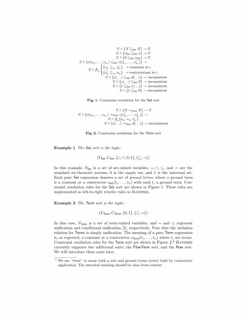
C ∧ {X ⊆Set X} → C

C ∧ {eSet ⊆Set 1} → C

C ∧ {0 ⊆Set eSet} → C

C ∧ {c(es1 , . . . , esn) ⊆Set c(e′s1 , . . . , e′

sn)} →

C ∧V

i

({esi ⊆si e′

si} c covariant in i

{e′si ⊆si esi} c contravariant in i

C ∧ {c(. . .) ⊆Set d(. . .)} → inconsistentC ∧ {c(. . .) ⊆Set 0} → inconsistentC ∧ {1 ⊆Set c(. . .)} → inconsistent

C ∧ {1 ⊆Set 0} → inconsistent

Fig. 1. Constraint resolution for the Set sort

C ∧ {X =Term X} → C

C ∧ {c(es1 , . . . , esn) =Term c(e′s1 , . . . , e′

sn)} →C ∧

Vi{esi =si e′

si}C ∧ {c(. . .) =Term d(. . .)} → inconsistent

Fig. 2. Constraint resolution for the Term sort

Example 1 The Set sort is the tuple:

(VSet, CSet, {∪,∩, 0, 1}, {⊆,=})

In this example, VSet is a set of set-valued variables, ∪,∩, ⊆, and = are thestandard set-theoretic notions, 0 is the empty set, and 1 is the universal set.Each pure Set expression denotes a set of ground terms, where a ground termis a constant or a constructor cSet(t1, . . . , tn) with each ti a ground term. Con-straint resolution rules for the Set sort are shown in Figure 1. These rules areimplemented as left-to-right rewrite rules in Banshee.

Example 2 The Term sort is the tuple:

(VTerm, CTerm, {0, 1}, {≤,=})

In this case, VTerm is a set of term-valued variables, and = and ≤ representunification and conditional unification [5], respectively. Note that the inclusionrelation for Terms is simply unification. The meaning of a pure Term expressionis, as expected, a constant or a constructor cTerm(t1, . . . , tn) where ti are terms.Constraint resolution rules for the Term sort are shown in Figure 2.4 Bansheecurrently supports two additional sorts: the FlowTerm sort, and the Row sort.We will introduce these sorts later.

4 We use “term” to mean both a sort and ground terms (trees) built by constructorapplication. The intended meaning should be clear from context.

2.2 Constraint Graphs

A system of mixed constraints can be represented as a directed graph wherethe nodes of the graph are expressions and the edges denote atomic constraintsbetween expressions. A constraint is atomic if either the left- or right-hand sideis a variable expression. To solve a system of mixed constraints, the constraintgraph is closed under the resolution rules for each sort (e.g. the rules in Figures 1and 2) as well as a transitive closure rule. Viewing a mixed constraint systemas a graph in this way, the resolution and transitive closure rules are essentiallydescriptions of how to add new edges to the constraint graph based on theexisting edges.

3 Specialization

This section describes the compilation strategy used in Banshee. The compila-tion process itself is straightforward, so we omit the low-level details and focusinstead on explaining the advantages of our approach.

The Banshee system has two main components: a code generator, and ageneric constraint resolution back-end. To use Banshee, the analysis designerwrites a specification file defining the constructor signatures for the analysis. Thecode generator reads the specification file and generates C code containing thespecialized components of the constraint engine. This C code is linked togetherwith the generic back-end to produce a specialized constraint resolution engine.

The key observation is that most analyses rely on a small, fixed numberof constructors, and because few analyses change their abstraction at run time,constructor signatures can be specified statically. Banshee uses these signaturesto implement customized versions of the constraint resolution rules such as theones shown in Figures 1 and 2.

Knowing the signatures of the constructors enables a host of static checksthat are not possible if new constructors are introduced at run time. To seethis, consider the constructor signature as a restricted programming language.This language specifies how to build expressions with the constructor (encodedby the arity of the constructor and the types of its component expressions),and how constraints between expressions matching the constructor should beresolved (encoded by the sort and variance of each of its component expressions).From this perspective, allowing dynamic constructors necessitates an interpreterfor the language of constructor signatures (this is essentially what Bane is).Specialization compiles the functionality encoded in a signature into C code,eliminating the overhead and runtime checking of an interpreter.

For a concrete example, consider the signature of a constructor fun intendedto model a function type in a unification-based type inference system. To makethe example more interesting, we add an additional component to the signatureto track the function’s latent effects, in the style of a type and effect system.The signature of the constructor is as follows:

fun : Term ∗ Term ∗ Set → Term

This signature can be specified in Banshee as follows (see Section 6 for a moredetailed explanation of this syntax):

data l_type : term = fun of l_type * l_type * effectand effect : set

Now suppose this signature was not fixed until runtime, and consider thecode to build a fun expression from a list of component expressions. This codemust ensure that the component expressions match the signature of the con-structor, which entails a number of dynamic checks. First, the code must checkthe number of component expressions to see that they match the arity of theconstructor. Next, the code must check the sort of each component expressionin the list, checking that the list as a whole matches the signature. In contrast,consider the same function in Banshee, where the constructor’s signature isknown statically. From this signature, Banshee generates a C function with thefollowing prototype:

l_type fun(l_type e0, l_type e1, effect e2)

Notice that the dynamic arity and sort checks are no longer necessary—theC type system guarantees that calls to this function have the correct number ofarguments (the arity check) and that the types of any actuals match the formalarguments (the sort checks).

As another example, consider implementing the rule for resolving constraintsbetween two fun expressions:

C ∧ {fun(eTerm1 , eTerm2 , eSet) =Term fun(e′Term1, e′Term2

, e′Set)} →C ∧ {eTerm1 =Term e′Term1

} ∧ {eTerm2 =Term e′Term2} ∧ {eSet =Set e′Set}

Banshee generates code for the above rule given the signature for thefun constructor. In contrast, the non-specialized approach must implement thegeneric rule for constructor matching shown in Figure 2. Implementing thegeneric rule requires: (1) calling the correct constraint relation for each com-ponent based on the sorts specified in the signature and (2) choosing the correctdirectionality based on the variances specified in the signature. If constructorsignatures are not known ahead of time, (1) requires either dynamic dispatch ora conditional to select the correct constraint relation and (2) requires a condi-tional to check the variance of the each argument. Banshee’s specialized versionof the rule avoids these inefficiencies.

We claim that one of the most important advantages of our specializationapproach is that it produces more maintainable code than the generic approach.The specialized code is easier to read, and permits modifications to the sourcespecification without causing wholesale changes to the handwritten part of theanalysis, as we will see in the case study (Section 6).

4 Incremental Analysis

In this section we describe Banshee’s support for a limited form of incrementalanalysis via backtracking. We believe that our use of backtracking as a mechanism

for incrementalizing static analyses is novel, as is the idea of adding backtrackingto a mixed constraint solver.

We assume a setting where constraints can be added to or deleted fromthe constraint system. In addition, queries to the constraint system can be in-terleaved arbitrarily between addition and deletion operations. Since our con-straint solver is online, additions are handled without any additional machinery(the trick is handling constraint deletions). Informally, we define an incrementalalgorithm as an algorithm that updates its output in response to program editswithout recomputing the analysis from scratch. In this setting, we call an incre-mental algorithm optimal if it never deletes (in other words, is never forced torediscover) an atomic constraint that is part of the updated solution in responseto a deletion operation. We also make the distinction between a top level atomicconstraint, which is a constraint that has been introduced to the system by anaddition operation, and an induced atomic constraint, which is a constraint thatis added as a consequence of the resolution rules.

4.1 An Optimal Algorithm

We begin by motivating our decision not to implement an optimal incrementalalgorithm in Banshee. We outline an algorithm, then illustrate the problemswith it.

The key to implementing an optimal incremental algorithm is to maintainexplicit dependency information. Besides adding edges to the constraint graph,the algorithm must keep track of the reasons why each edge was added. Oneway to do this is to maintain a list of the edges in the graph that triggeredeach new edge addition. When a constraint is deleted, all occurrences of thecorresponding edge in the constraint graph are removed from the dependencylist. An empty dependency list means that all of the reasons an edge was addedhave been removed, and hence, that constraint should be removed. This processis repeated until no more constraints are removed.

We demonstrate these ideas with a simple example. Suppose the constraints

X ⊆ Y1 (1)X ⊆ Y2 (2)Y2 ⊆ Z1 (3)

are added to an initially empty constraint system. By transitive closure, thelatter two constraints would trigger the constraint

X ⊆ Z1 (4)

The incremental solver adds the entry (2,3) to the dependency list for con-straint 4. This records the fact that the presence of constraints 2 and 3 togethertriggered the addition of constraint 4. If either constraint were deleted, constraint4 should be deleted as well (unless there is some other entry in the dependency

Y1 8

��

^ ] Z U M<

+5

��X

1

77

4

JJ3L

W _ g r�7

HH<W Z \ ^ _ ` b d h �2

// Y23 // Z1

6 // Z2

(a)

Edge Dependencies

4 (2,3), (1,5)

7 (4,6), (1,8)

8 (5,6)

(b)

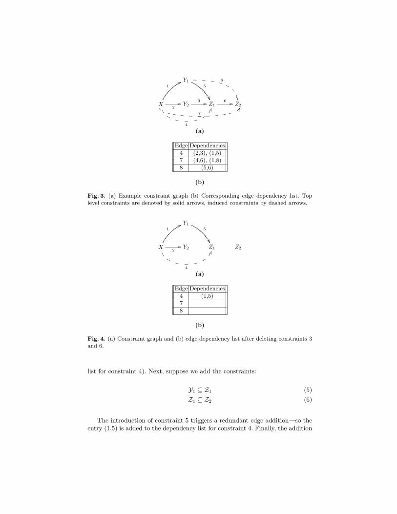
Fig. 3. (a) Example constraint graph (b) Corresponding edge dependency list. Toplevel constraints are denoted by solid arrows, induced constraints by dashed arrows.

Y1

5

��X

1

77

4

JJ3L

W _ g r�

2// Y2 Z1 Z2

(a)

Edge Dependencies

4 (1,5)

7

8

(b)

Fig. 4. (a) Constraint graph and (b) edge dependency list after deleting constraints 3and 6.

list for constraint 4). Next, suppose we add the constraints:

Y1 ⊆ Z1 (5)Z1 ⊆ Z2 (6)

The introduction of constraint 5 triggers a redundant edge addition—so theentry (1,5) is added to the dependency list for constraint 4. Finally, the addition

of constraint (6) causes the constraints

X ⊆ Z2 (7)Y1 ⊆ Z2 (8)

to be added, with (4,6) and (1,8) added to the dependency list for constraint 7.Figure 3 shows the constraint graph and edge dependency list at this point inthe example.

Now suppose we delete constraints 3 and 6 from the system, in that order.Deleting constraint 3 removes the entry (2,3) from the edge dependency list forconstraint 4. However, the dependency list for constraint 4 is non-empty, so we donot remove it from the system. Deleting constraint 6 removes the entries (4,6)and (5,6) from the edge dependency table. Since constraints 7 and 8 have anempty dependency list, they are deleted from the constraint system. Notice thatfor correctness this algorithm must store every set of edges that may cause anedge to be added. Thus, the algorithm must maintain extra information even forredundant edge additions. While much work has been done to reduce redundantedge additions, constraint solvers still add many redundant edges to the graph[6]. Having to store extra information on each redundant edge addition wouldhinder the scalability of the constraint solver.

A more practical concern is the engineering effort required to support anoptimal incremental analysis. While efforts have been made to factor out in-crementality at the data structure level, there does not seem to be a practical,general solution for arbitrary data structures [7]. Adding ad-hoc support for in-cremental updates to each sort in Banshee is a daunting task, especially sincethe solver algorithms use highly optimized representations. As an example, ourset constraint solver implements partial online cycle elimination, which uses aunion-find data structure internally [8]. Adding incremental support to just thefast union find algorithm is not easy—in fact, some of the published solutionsare incorrect (see [9] for a discussion).

4.2 Backtracking

Instead of implementing a fully incremental analysis, we have added backtrackingto Banshee. Backtracking allows a constraint system to be rolled back to anyprevious state. In this subsection, we explain the general approach to addingbacktracking, and discuss the practical advantages of backtracking over optimalincremental analysis.

Backtracking is based on a simple approximation of edge dependencies:each induced constraint is assumed to be dependent on the all of the con-straints introduced into the constraint system earlier. This seemingly gross over-approximation yields a simple strategy for handling constraint deletions: wesimply delete all of the constraints added to the system after the constraint wewish to delete. Then we add back any top level constraints we didn’t intend todelete, and allow the constraint solver to solve for any induced constraints weshouldn’t have removed.

Operationally, this strategy can be implemented simply by time stampingeach atomic constraint in the system. To delete constraint i, we perform a scanof all the edges in the constraint graph, deleting any edge whose timestamp isgreater than i. Then we simply add back all the top level constraints timestampedj with j > i. Referring to our example in Figures 3 and 4, we see that deletingconstraint 6 triggers the deletion of constraints 7 and 8 (in this case, backtrackingdoes no more work than the optimal analysis). Deleting constraint 3, on the otherhand, forces us to delete constraints 5 and 4. We will have to re-introduce thetop level constraint 5 and solve to re-discover the induced constraint 4.

While backtracking is clearly not an optimal incremental technique, it doeshave a number of practical advantages over the optimal algorithm. First, back-tracking is fast: it can be accomplished in a linear scan over the edges in theconstraint graph. Second, the storage overhead to support backtracking is min-imal, requiring only a timestamp per edge.

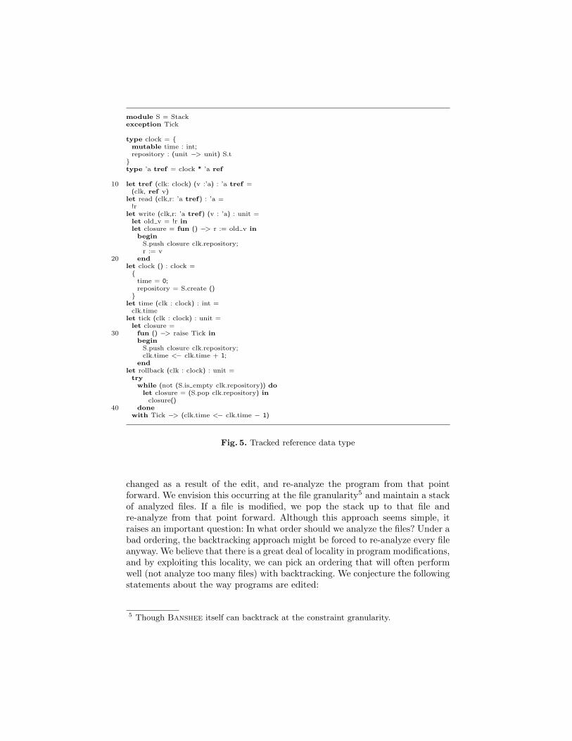
In addition, we have devised a new data type called a tracked reference thatallows us to add efficient backtracking support to general data structures. Thishas greatly simplified the task of incorporating backtracking into Banshee’salgorithms, especially in the presence of optimizations like cycle elimination andprojection merging [8, 6]. A tracked reference is essentially a mutable referencethat maintains a repository of its old versions. Each tracked reference is tiedto a clock; each tick of the clock checkpoints the reference’s state. When theclock is rolled back, the previous state is restored. Rolling back is a destructiveoperation. Figure 5 contains a compilable OCaml implementation of the trackedreference data type. The implementation keeps a stack of closures containing theold reference contents. Invoking a closure restores the old contents. A backtrack-ing operation simply pops entries off the stack until the previous recorded clocktick.

In a functional language, adding support for backtracking to a data structureis simple: it suffices to replace all references with tracked references and add callsto the clock’s tick function when a checkpoint is desired. Obvious inefficienciesarise, however, if tracked references are applied carelessly. In general, they shouldbe applied so as to avoid storing copies of large objects in the closures. AlthoughBanshee is implemented in C rather than a functional language, we imple-mented backtracking by applying the tracked reference concept systematicallyto each data structure. Interestingly, we do not pay in any way for this factor-ing: there are no “tricks” that are obscured by applying the tracked referenceidea generally. For example, applying tracked references to a standard union-findalgorithm yields an algorithm that is equivalent to a well-known algorithm forunion-find with backtracking [10].

4.3 Static Analysis with Backtracking

We have shown that backtracking is both efficient and easy to implement, butwe have not shown how to use the technique to incrementalize static analyses.The basic approach is as follows: given that we have fully analyzed a program,in response to a program edit we can backtrack to the earliest constraint that

module S = Stackexception Tick

type clock = {mutable time : int;repository : (unit −> unit) S.t

}type ’a tref = clock * ’a ref

10 let tref (clk: clock) (v :’a) : ’a tref =(clk, ref v)

let read (clk,r: ’a tref) : ’a =!r

let write (clk,r: ’a tref) (v : ’a) : unit =let old v = !r inlet closure = fun () −> r := old v inbegin

S.push closure clk.repository;r := v

20 endlet clock () : clock ={

time = 0;repository = S.create ()

}let time (clk : clock) : int =

clk.timelet tick (clk : clock) : unit =let closure =

30 fun () −> raise Tick inbegin

S.push closure clk.repository;clk.time <− clk.time + 1;

endlet rollback (clk : clock) : unit =trywhile (not (S.is empty clk.repository)) dolet closure = (S.pop clk.repository) in

closure()40 done

with Tick −> (clk.time <− clk.time − 1)

Fig. 5. Tracked reference data type

changed as a result of the edit, and re-analyze the program from that pointforward. We envision this occurring at the file granularity5 and maintain a stackof analyzed files. If a file is modified, we pop the stack up to that file andre-analyze from that point forward. Although this approach seems simple, itraises an important question: In what order should we analyze the files? Under abad ordering, the backtracking approach might be forced to re-analyze every fileanyway. We believe that there is a great deal of locality in program modifications,and by exploiting this locality, we can pick an ordering that will often performwell (not analyze too many files) with backtracking. We conjecture the followingstatements about the way programs are edited:

5 Though Banshee itself can backtrack at the constraint granularity.

1. Developers do not make sweeping, system wide changes to mature projectsvery frequently: most modifications touch a small number of files. Therefore,for a given change, most of the files in a project remain unchanged.

2. Libraries and utility files are modified infrequently.3. Recently modified files are more likely to be modified than other files.

We describe two strategies for picking a stack ordering based on these conjec-tures. Both assume that the first conjecture holds. The first strategy attempts toexploit the second conjecture; the second strategy attempts to exploit the third.

In the first strategy, we build a dependency graph for the project and use alinearization (using a canonical linearization strategy) of the graph as the stackorder. When a source file changes, we compute a new dependency graph and lin-earization, and pop the stack down to a common prefix of the two linearizations.This approach attempts to keep libraries and utilities at the bottom of the stack.In addition, by utilizing dependency graphs, this strategy tries to minimize thedeletion of edges that aren’t relevant to the program edit.

The second strategy is based on the conjecture that recently modified filesare more likely to be modified than other files. Under this strategy, the sourcefiles are initially analyzed in an arbitrary order. When a file is modified, thestack is popped down to that file. Now, when replacing the files back onto thestack, the file that was actually modified is placed on top of the stack, in thehopes that it is the next file to be modified. If this assumption holds, we willonly have to re-analyze that file. Otherwise, the file will at least be close to thetop of the stack in the case that it is modified again soon.

5 Persistence

In this section, we briefly explain our approach to making Banshee’s constraintsystems persistent. Persistence is a useful feature to have when incorporating in-cremental analyses into standard build processes. We require persistence (ratherthan a feature to save and load in some simpler format) because we need toreconstruct the complete representations of our data structures to support back-tracking and online constraint solving.

To support persistent constraint systems, we added serialization and deserial-ization capabilities to the region-based memory management library that Ban-shee uses for memory allocation. This approach allows us to save constraintsystems by serializing a collection of regions, and load a constraint system bydeserializing regions and updating any pointer values stored in the regions. Ini-tially, we implemented serialization using a standard pointer tracing approach,but found this strategy to be too slow. Region-based serialization allows us tosimply write sequential pages of memory to disk, which we found to be two or-ders of magnitude faster than pointer tracing. With region-based serialization,we are able to serialize a 170 MB constraint graph in 2.4 seconds, vs. 30 secondsto serialize the same graph by tracing pointers.

Region-based memory management is also a good fit for our backtrackingproposal. One effective strategy is to create a new region for each file being ana-

lyzed and allocate new objects in that region. When backtracking, any obsoleteregions can be freed. In addition, if we know before loading a saved constraintsystem that a backtrack operation will take place immediately after the load,we can selectively deserialize only the live regions of memory (assuming that themetadata for backtracking is stored in a different set of regions that is deserial-ized).

6 Case Study: Points-to Analysis

We continue with several realistic examples derived from points-to analyses wehave formulated in Banshee. Our goal is to show how Banshee can be used toexplore different design points and prototype several variations of a given pro-gram analysis. In the first three examples, we refine the degree of subtyping usedin the points-to analysis. Much of the recent research on points-to analysis hasfocused on this issue [5, 11, 12]. In the last example, we show how to augmentthe points-to analysis to perform receiver class analysis in an object-orientedlanguage with explicit pointer manipulations (e.g. C++). This last analysis isinteresting as it computes the call graph on the fly during the points-to computa-tion, instead of using a pre-computed call graph obtained from a coarser analysis(e.g. class hierarchy analysis). We conclude with a brief discussion of other de-sign points that can be explored with Banshee, including polymorphism andfield sensitivity.

6.1 Andersen’s Analysis

We begin by examining a set-based formulation of Andersen’s points-to analysisbuilt with Banshee. The analysis constructs a points-to graph from a set ofabstract memory locations {`1, . . . , `n} and set variables X`1 , . . . ,X`n .

Intuitively, we model a reference as an object with an abstract location andmethods get : void → X`x

and set : X`x→ void, where X`x

represents the points-to set of the location. Updating the location corresponds to applying the setfunction to the new value. Dereferencing a location corresponds to applying theget function. In our vocabulary of Set expressions, references are modeled witha constructor ref containing three fields: a constant `x representing the abstractlocation, a covariant field X`x representing the get function, and a contravariantfield X `x representing the set function.

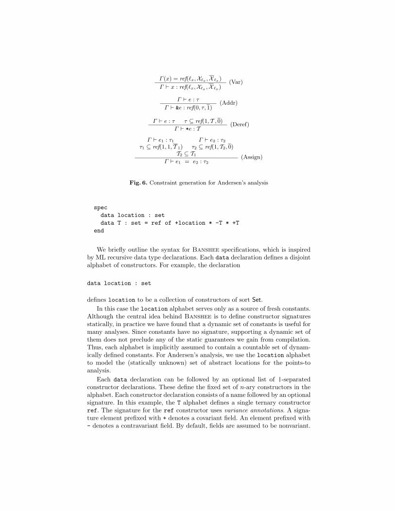
Figure 6 shows a subset of the inference rules for Andersen’s analysis. Thetype judgments assign a set expression to each program expression, possiblygenerating some side constraints. To avoid having separate rules for l-values andr-values, each type judgment infers a set denoting an l-value. Hence, the setexpression in the conclusion of (Var) denotes the location of program variablex, rather than its contents.

In Banshee, Andersen’s analysis is defined with the following specification:

specification andersen : ANDERSEN =

Γ (x) = ref(`x,X`x ,X `x)

Γ ` x : ref(`x,X`x ,X `x)(Var)

Γ ` e : τ

Γ ` &e : ref(0, τ, 1)(Addr)

Γ ` e : τ τ ⊆ ref(1, T , 0)

Γ ` *e : T(Deref)

Γ ` e1 : τ1 Γ ` e2 : τ2

τ1 ⊆ ref(1, 1, T 1) τ2 ⊆ ref(1, T2, 0)T2 ⊆ T1

Γ ` e1 = e2 : τ2

(Assign)

Fig. 6. Constraint generation for Andersen’s analysis

specdata location : setdata T : set = ref of +location * -T * +T

end

We briefly outline the syntax for Banshee specifications, which is inspiredby ML recursive data type declarations. Each data declaration defines a disjointalphabet of constructors. For example, the declaration

data location : set

defines location to be a collection of constructors of sort Set.In this case the location alphabet serves only as a source of fresh constants.

Although the central idea behind Banshee is to define constructor signaturesstatically, in practice we have found that a dynamic set of constants is useful formany analyses. Since constants have no signature, supporting a dynamic set ofthem does not preclude any of the static guarantees we gain from compilation.Thus, each alphabet is implicitly assumed to contain a countable set of dynam-ically defined constants. For Andersen’s analysis, we use the location alphabetto model the (statically unknown) set of abstract locations for the points-toanalysis.

Each data declaration can be followed by an optional list of |-separatedconstructor declarations. These define the fixed set of n-ary constructors in thealphabet. Each constructor declaration consists of a name followed by an optionalsignature. In this example, the T alphabet defines a single ternary constructorref. The signature for the ref constructor uses variance annotations. A signa-ture element prefixed with + denotes a covariant field. An element prefixed with- denotes a contravariant field. By default, fields are assumed to be nonvariant.

6.2 Steensgaard’s Analysis

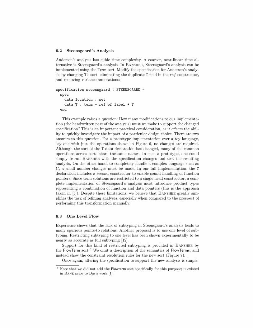
Andersen’s analysis has cubic time complexity. A coarser, near-linear time al-ternative is Steensgaard’s analysis. In Banshee, Steensgaard’s analysis can beimplemented using the Term sort. Modify the specification for Andersen’s analy-sis by changing T’s sort, eliminating the duplicate T field in the ref constructor,and removing variance annotations:

specification steensgaard : STEENSGAARD =specdata location : setdata T : term = ref of label * T

end

This example raises a question: How many modifications to our implementa-tion (the handwritten part of the analysis) must we make to support the changedspecification? This is an important practical consideration, as it effects the abil-ity to quickly investigate the impact of a particular design choice. There are twoanswers to this question. For a prototype implementation over a toy language,say one with just the operations shown in Figure 6, no changes are required.Although the sort of the T data declaration has changed, many of the commonoperations across sorts share the same names. In such a prototype, one couldsimply re-run Banshee with the specification changes and test the resultinganalysis. On the other hand, to completely handle a complex language such asC, a small number changes must be made. In our full implementation, the Tdeclaration includes a second constructor to enable sound handling of functionpointers. Since term solutions are restricted to a single head constructor, a com-plete implementation of Steensgaard’s analysis must introduce product typesrepresenting a combination of function and data pointers (this is the approachtaken in [5]). Despite these limitations, we believe that Banshee greatly sim-plifies the task of refining analyses, especially when compared to the prospect ofperforming this transformation manually.

6.3 One Level Flow

Experience shows that the lack of subtyping in Steensgaard’s analysis leads tomany spurious points-to relations. Another proposal is to use one level of sub-typing. Restricting subtyping to one level has been shown experimentally to benearly as accurate as full subtyping [12].

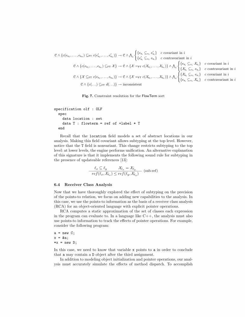
Support for this kind of restricted subtyping is provided in Banshee bythe FlowTerm sort.6 We omit a description of the semantics of FlowTerms, andinstead show the constraint resolution rules for the new sort (Figure 7).

Once again, altering the specification to support the new analysis is simple:

6 Note that we did not add the Flowterm sort specifically for this purpose; it existedin Bane prior to Das’s work [1].

C ∧ {c(es1 , . . . , esn) ⊆FT c(e′s1 , . . . , e′

sn)} → C ∧V

i

({esi ⊆si e′

si} c covariant in i

{e′si ⊆si esi} c contravariant in i

C ∧ {c(es1 , . . . , esn) ⊆FT X} → C ∧ {X =FT c(Xs1 , . . . ,Xsn)} ∧V

i

({esi ⊆si Xsi} c covariant in i

{Xsi ⊆si esi} c contravariant in i

C ∧ {X ⊆FT c(es1 , . . . , esn)} → C ∧ {X =FT c(Xs1 , . . . ,Xsn)} ∧V

i

({Xsi ⊆si esi} c covariant in i

{esi ⊆si Xsi} c contravariant in i

C ∧ {c(. . .) ⊆FT d(. . .)} → inconsistent

Fig. 7. Constraint resolution for the FlowTerm sort

specification olf : OLFspecdata location : setdata T : flowterm = ref of +label * T

end

Recall that the location field models a set of abstract locations in ouranalysis. Making this field covariant allows subtyping at the top level. However,notice that the T field is nonvariant. This change restricts subtyping to the toplevel: at lower levels, the engine performs unification. An alternative explanationof this signature is that it implements the following sound rule for subtyping inthe presence of updateable references [13]:

`x ⊆ `y X`x= X`y

ref(`x,X`x) ≤ ref(`y,X`y

)(sub-ref)

6.4 Receiver Class Analysis

Now that we have thoroughly explored the effect of subtyping on the precisionof the points-to relation, we focus on adding new capabilities to the analysis. Inthis case, we use the points-to information as the basis of a receiver class analysis(RCA) for an object-oriented language with explicit pointer operations.

RCA computes a static approximation of the set of classes each expressionin the program can evaluate to. In a language like C++, the analysis must alsouse points-to information to track the effects of pointer operations. For example,consider the following program:

a = new C;x = &a;*x = new D;

In this case, we need to know that variable x points to a in order to concludethat a may contain a D object after the third assignment.

In addition to modeling object initialization and pointer operations, our anal-ysis must accurately simulate the effects of method dispatch. To accomplish

these tasks, new constructors representing class definitions and dispatch tablesare added to our points-to analysis specification.

For simplicity, we assume that methods in this language have a single formalargument in addition to the implicit this parameter. We also assume that theinheritance tree for the program has been flattened as a preprocessing step, suchthat if class B extends A, B contains definitions for methods in A not overriddenin B. Here is the Banshee specification for this example, assuming we choseAndersen’s analysis as our base points-to analysis:

specification rca : RCA =specdata location : setdata T : set = ref of +location * -T * +T

| class of +location * +dispatchand dispatch : row(method)and method : set = fun of -T * -T * +T

end

The class constructor contains a location field containing the name of theclass and a dispatch field representing the dispatch table for objects of thatclass. Notice that dispatch uses a new sort: the Row sort. We first explain howthis abstraction is intended to work before describing the Row sort.

We model an object’s dispatch table as a collection of methods (each inturn modeled by the method constructor) indexed by name. Given a dispatchexpression like e.foo(), our analysis should compute the set of classes that emay evaluate to, search each class’s dispatch table for a method named foo, andexecute it (abstractly) if it exists. Methods are modeled by the fun constructor.Methods model the implicit this parameter with the first T field, the singleformal parameter by the second T field, and a single return value by the third Tfield. Recall that the function constructor must be contravariant in its domainand covariant in its range, as reflected in the specification.

For this approach to work, our dispatch table abstraction must maintain amapping between method names and method terms. This mapping is accom-plished using the Row sort. A Row of base sort s (written Row(s)) denotes apartial function from an infinite set of names to terms of sort s. Row expressionsare used to model record types with width and depth subtyping. We omit fur-ther details of the Row sort here: for this example, it suffices to view rows asmappings between names and terms.

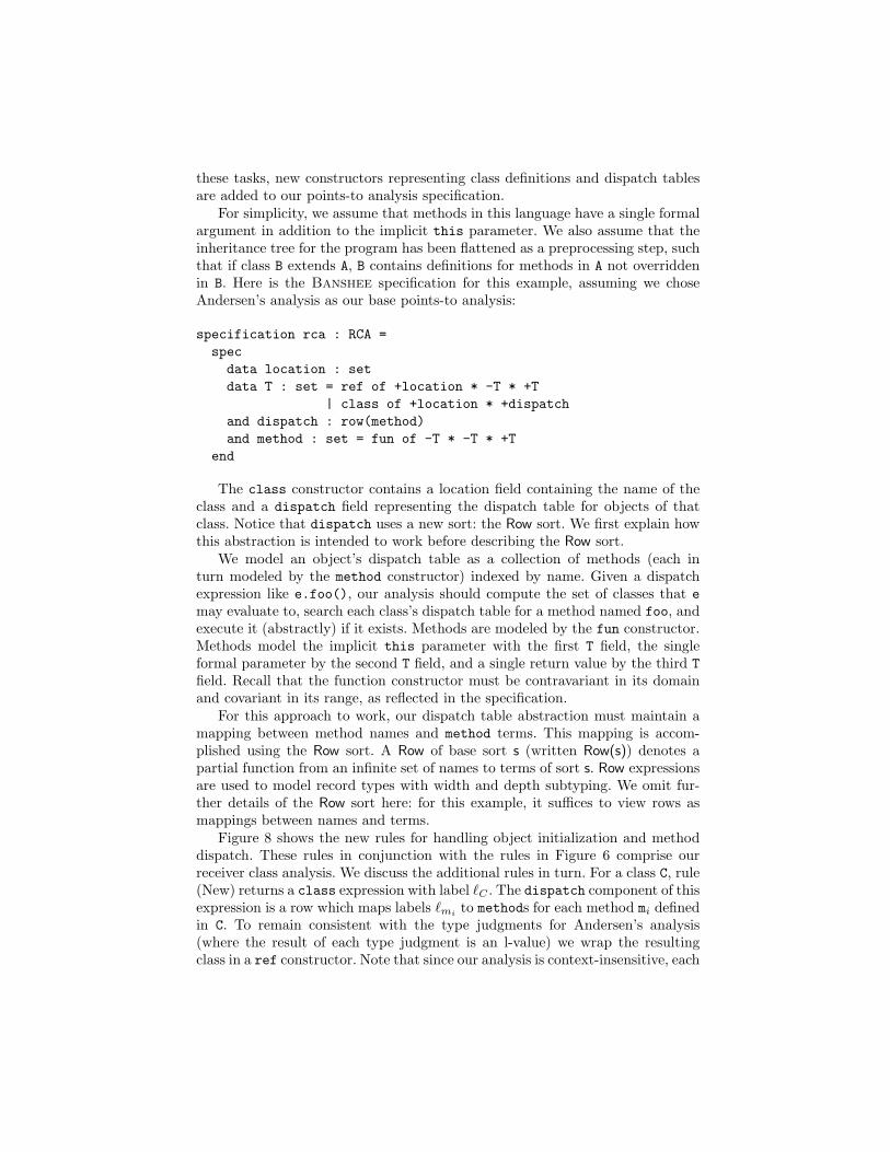
Figure 8 shows the new rules for handling object initialization and methoddispatch. These rules in conjunction with the rules in Figure 6 comprise ourreceiver class analysis. We discuss the additional rules in turn. For a class C, rule(New) returns a class expression with label `C . The dispatch component of thisexpression is a row which maps labels `mi

to methods for each method mi definedin C. To remain consistent with the type judgments for Andersen’s analysis(where the result of each type judgment is an l-value) we wrap the resultingclass in a ref constructor. Note that since our analysis is context-insensitive, each

Γ ` new C : ref(0, class(`C , < `mi : fun(Xthis,Xarg,Xret) . . . >), 1)(New)

Γ ` e1 : τ1 Γ ` e2 : τ2

τ1 ⊆ ref(1, T1, 0) τ2 ⊆ ref(1, T2, 0)T1 ⊆ class(1, < `m : fun(T1, T2, Tret) . . . >)

Γ ` e1.m(e2) : ref(0, Tret, 1)(Dispatch)

Fig. 8. Rules for receiver class analysis (add to the rules from Figure 6).

instance of new C occurring in the program yields the same class expression,which is created when the definition of C is analyzed. In (Dispatch), e1 is analyzedand assumed to contain a set of classes7. For each class which defines a methodnamed m (i.e. the associated dispatch row contains a mapping for label `m), thecorresponding method body is selected, and constrained such that the actualparameters flow into the formal parameters, and the return value of the function(lifted to an l-value) is the result of the entire expression.

This specification takes advantage of Banshee’s strong type system. WithBanshee’s compilation approach, the type of method expressions is incompat-ible with the type of T expressions, despite the fact that both are kinds of Setexpressions. Thus, Banshee eliminates the possibility of (e.g.) a class abstrac-tion appearing in a dispatch table.

6.5 Other Design Points

Points-to analyses can be classified by dimensions other than the degree of sub-typing. We note that it is possible to explore these additional dimensions andexpress other interesting analyses using Banshee. For example, field-sensitiveanalyses can be defined using Banshee’s Row sort to model structures. Poly-morphic recursive analyses can be implemented using a library for context-freelanguage reachability that has been built on top of Banshee [14].

7 Experiments

7.1 Scalability and Performance

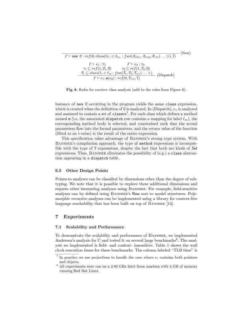
To demonstrate the scalability and performance of Banshee, we implementedAndersen’s analysis for C and tested it on several large benchmarks8. The anal-ysis we implemented is field- and context- insensitive. Table 1 shows the wallclock execution times for these benchmarks. The column labeled “TLB time” is7 In practice we use projections to handle the case where e1 contains both pointers

and objects.8 All experiments were run on a 2.80 GHz Intel Xeon machine with 4 GB of memory

running Red Hat Linux.

Benchmark Description Preproc LOC Analysis Time(s) TLB time(s)

gs Ghostscript 437211 3.3 3.6

spice Circuit simulation program 849258 1.5 1.5

pgsql PostgreSQL 1322420 5.3 .74

gimp Gnu Image Manipulation Program 7472553 18.0 2.2

linux Linux kernel v2.4 (default config) 3784959 41.1 13.4Table 1. Benchmark data for Andersen’s analysis

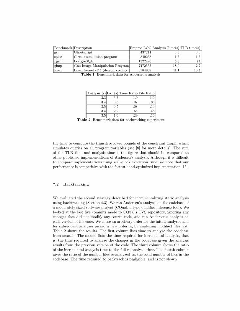
Analysis (s) Inc. (s) Time Ratio File Ratio

3.3 3.3 1.0 1.0

3.4 3.3 .97 .88

3.5 0.5 .08 .14

3.4 2.2 .65 .48

3.5 1.0 .29 .10Table 2. Benchmark data for backtracking experiment

the time to compute the transitive lower bounds of the constraint graph, whichsimulates queries on all program variables (see [8] for more details). The sumof the TLB time and analysis time is the figure that should be compared toother published implementations of Andersen’s analysis. Although it is difficultto compare implementations using wall-clock execution time, we note that ourperformance is competitive with the fastest hand-optimized implementation [15].

7.2 Backtracking

We evaluated the second strategy described for incrementalizing static analysisusing backtracking (Section 4.3). We ran Andersen’s analysis on the codebase ofa moderately sized software project (CQual, a type qualifier inference tool). Welooked at the last five commits made to CQual’s CVS repository, ignoring anychanges that did not modify any source code, and ran Andersen’s analysis oneach version of the code. We chose an arbitrary order for the initial analysis, andfor subsequent analyses picked a new ordering by analyzing modified files last.Table 2 shows the results. The first column lists time to analyze the codebasefrom scratch. The second lists the time required for incremental analysis, thatis, the time required to analyze the changes in the codebase given the analysisresults from the previous version of the code. The third column shows the ratioof the incremental analysis time to the full re-analysis time. The fourth columngives the ratio of the number files re-analyzed vs. the total number of files in thecodebase. The time required to backtrack is negligible, and is not shown.

8 Related Work

We discuss two threads of related work: frameworks and toolkits comparable toset constraints, and work related to incremental analysis.

There are several frameworks whose expressive power is similar to that ofthe mixed constraint framework presented here. Datalog is a database querylanguage based on logic programming [16]. Datalog has recently received someattention as a specification language for static analyses. We note that the subsetof pure set constraints implemented in Banshee is equivalent to chain data-log [17] and also context-free language reachability [18]. There are also obviousconnections to bottom-up logic [19].

Implementations of these frameworks have been applied to solve static anal-ysis problems. The bddbddb system is a deductive database that uses a binary-decision diagram library as its back-end [20]. Using Datalog as a high levellanguage, bddbddb hides low-level BDD operations from the analysis designer.Other toolkits that use BDD back-ends include CrocoPat [21] and Jedd [22]. Anefficient algorithm for Dyck context-free language reachability has been shownto be useful for solving various flow analysis problems [23]. A demand-drivenversion of the algorithm also exists [24], though we have not so far seen a fullyincremental algorithm described. We note that our description of an optimalincremental algorithm (as well as our backtracking algorithm) apply to Dyck-CFLR problems via a reduction described in previous work [14].

Ramalingam and Reps have compiled a categorized bibliography on incre-mental computation [25]. We are not aware of previous work on incrementalizingset constraints, though work on incrementalizing transitive closure is abundantand addresses some of the same issues [26, 27]. The CLA (compile, link, analyze)[15] approach to analyzing large codebases supports a form of file-granularityincrementality similar to traditional compilers: modified files can be re-compiledand linked to any unchanged object files. This approach has some advantages.For example, since CLA doesn’t save any analysis results, object file formatsare simpler, and there is no need to make the analysis persistent. However, CLAdefers all of its analysis work until after the link phase, so the only savings wouldbe the cost of parsing and producing the object files.

References

1. Aiken, A., Fahndrich, M., Foster, J., Su, Z.: A Toolkit for Constructing Type- andConstraint-Based Program Analyses. In: Proceedings of the Second InternationalWorkshop on Types in Compilation (TIC’98). (1998)

2. Ragan-Kelley, J.: Practical Interactive Lighting Design for RenderMan Scenes.Undergraduate Thesis (2004)

3. Ragan-Kelley, J. Personal communication (2004)

4. Fahndrich, M.: BANE: A Library for Scalable Constraint-Based Program Anal-ysis . PhD dissertation, University of California, Berkeley, 1999., Department ofComputer Science (1999)

5. Steensgaard, B.: Points-to Analysis in Almost Linear Time. In: Proceedings of the23th Annual ACM SIGPLAN-SIGACT Symposium on Principles of ProgrammingLanguages. (1996) 32–41

6. Su, Z., Fahndrich, M., Aiken, A.: Projection Merging: Reducing Redundancies inInclusion Constraint Graphs. In: Proceedings of the 27th ACM SIGPLAN-SIGACTSymposium on Principles of Programming Languages, ACM Press (2000) 81–95

7. Driscoll, J.R., Sarnak, N., Sleator, D.D., Tarjan, R.E.: Making Data StructuresPersistent. J. Comput. Syst. Sci. 38 (1989) 86–124

8. Fahndrich, M., Foster, J.S., Su, Z., Aiken, A.: Partial Online Cycle Elimination inInclusion Constraint Graphs. In: Proceedings of the 1998 ACM SIGPLAN Con-ference on Programming Language Design and Implementation, Montreal, Canada(1998) 85–96

9. Galil, Z., Italiano, G.F.: A Note on Set Union with Arbitrary Deunions. Inf.Process. Lett. 37 (1991) 331–335

10. Westbrook, J., Tarjan, R.E.: Amortized analysis of algorithms for set union withbacktracking. SIAM J. Comput. 18 (1989) 1–11

11. Shapiro, M., Horwitz, S.: Fast and Accurate Flow-Insensitive Points-To Analy-sis. In: Proceedings of the 24th Annual ACM SIGPLAN-SIGACT Symposium onPrinciples of Programming Languages. (1997)

12. Das, M.: Unification-based pointer analysis with directional assignments. In: SIG-PLAN Conference on Programming Language Design and Implementation. (2000)35–46

13. Abadi, M., Cardelli, L.: A Theory of Objects. Springer (1996)14. Kodumal, J., Aiken, A.: The Set Constraint/CFL Reachability Connection in

Practice. In: Proceedings of the ACM SIGPLAN 2004 conference on Programminglanguage design and implementation, ACM Press (2004) 207–218

15. Heintze, N., Tardieu, O.: Ultra-fast Aliasing Analysis Using CLA: A Million Linesof C Code in a Second. In: SIGPLAN Conference on Programming LanguageDesign and Implementation. (2001) 254–263

16. Ceri, S., Gottlob, G., Tanca, L.: What You Always Wanted to Know About Dat-alog (And Never Dared to Ask). IEEE Transactions on Knowledge and DataEngineering 1 (1989) 146–166

17. Yannakakis, M.: Graph-theoretic methods in database theory. In: Proceed-ings of the Ninth ACM SIGACT-SIGMOD-SIGART Symposium on Principles ofDatabase Systems, ACM Press (1990) 230–242

18. Melski, D., Reps, T.: Interconvertbility of Set Constraints and Context-Free Lan-guage Reachability. In: Proceedings of the 1997 ACM SIGPLAN Symposium onPartial Evaluation and Semantics-based Program Manipulation, ACM Press (1997)74–89

19. McAllester, D.: On the complexity analysis of static analyses. J. ACM 49 (2002)512–537

20. Whaley, J., Lam, M.S.: Cloning-Based Context-Sensitive Pointer Alias AnalysisUsing Binary Decision Diagrams. In: Proceedings of the Conference on Program-ming Language Design and Implementation, ACM Press (2004)

21. Beyer, D., Noack, A., Lewerentz, C.: Simple and Efficient Relational Querying ofSoftware Structures. In: Proceedings of the 10th Working Conference on ReverseEngineering, IEEE Computer Society (2003) 216

22. Lhotak, O., Hendren, L.: Jedd: A BDD-based relational extension of Java. In:Proceedings of the ACM SIGPLAN 2004 Conference on Programming LanguageDesign and Implementation, ACM Press (2004)

23. Reps, T., Horwitz, S., Sagiv, M.: Precise Interprocedural Dataflow Analysis viaGraph Reachability. In: Proceedings of the 22nd Annual ACM SIGPLAN-SIGACTSymposium on Principles of Programming Languages, San Francisco, California(1995) 49–61

24. Horwitz, S., Reps, T., Sagiv, M.: Demand Interprocedural Dataflow Analysis. In:Proceedings of the 3rd ACM SIGSOFT Symposium on Foundations of SoftwareEngineering, ACM Press (1995) 104–115

25. Ramalingam, G., Reps, T.: A categorized bibliography on incremental computa-tion. In: Proceedings of the 20th ACM SIGPLAN-SIGACT symposium on Princi-ples of programming languages, ACM Press (1993) 502–510

26. Demetrescu, C., Italiano, G.F.: Fully Dynamic Transitive Closure: BreakingThrough the O(n2) Barrier. In: Proceedings of the 41st Annual Symposium onFoundations of Computer Science, IEEE Computer Society (2000) 381

27. Roditty, L.: A Faster and Simpler Fully Dynamic Transitive Closure. In: Pro-ceedings of the fourteenth annual ACM-SIAM symposium on Discrete algorithms,Society for Industrial and Applied Mathematics (2003) 404–412