BEHAVIORAL MACROECONOMICS VIA

SPARSE DYNAMIC PROGRAMMING

Xavier GabaixNYU, CEPR and NBER

June 2016

INTRODUCTION

I Normally, (1) we economists use a simplified model of theworld, knowing that the model is not literally the true world

I (2) But agents in our models are assumed to comprehend thefull complexity of their world.

I In this paper: (1) applies, but (2) is replaced by (2’): Agentsalso have a simplified sub-model of their world.

I I model and explore the consequences of that.I One payoff: do economics without the rational high-frequencyEuler equation, which anyway typically fails.

I PrinciplesI A vector m ∈ R1,000,000 is sparse if most entries are 0I The agent is like an economist, building a simplified — sparse— representation of the world

I The “vector”of attention will be sparse —people don’t thinkabout most things

LINK WITH HIGH-DIMENSIONAL ECONOMIES

I “High-dimensional economy”: with a large (but finite) numberof firms and sectors. Or with networks.

I “Granular”: you can’t analyze it with just the median firm.I If the economy is high-dimensional, then agents will find itdiffi cult to solve it in their head

I N firms: agents need to think about impact of each firm, ateach round, for each date.

I Decision-making in networks: if I re-link up with Thomas, Ishould evaluate the benefits down the road, including all thehigher-order impact in Thomas’network

I Clearly , we need to simplify that.I This sparsity framework might be useful.

RELATED LITERATURE

I Behavioral economics and financeI A lot of the literature is about modeling tastes or beliefsI There is less on the modeling of rationality itself: O’DonoghueRabin, k−level models, Crawford et al., Camerer Ho andChuong, Jéhiel et al., MacLeod, Hong and Stein, Koszegi andSzeidl, Schwartzstein, Fuster, Hébert and Laibson, Bordalo,Gennaioli and Shleifer...

I Finance / Macro:I Inattention: Sims 03, Gabaix and Laibson 02, 06, Mankiw Reis02, Reis 06, Chetty, Kroft Looney 09, Angeletos La’O 10,Mackowiak and Wiederholt 10, 16, Masatlioglu and Ok 10,Veldkamp 11, Matejka and Sims 11, Caplin, Dean and Martin11, Woodford 12, Alvarez Lippi, Paciello 13, Koszegi Szeidl 13,Abel, Eberly and Panageas 13, Greenwood Hanson 14, Croce,Lettau Ludvigson 15

I Early behavioral models: Campbell Mankiw 89

I Learning: Sargent 93, Evans and Honkapohja 01I Approximation: Krusell Smith 98, Judd 98

RELATED LITERATURE

I High-Dimensional economics and networks: Long Plosser ’83,Gabaix ’11, Acemoglu, Carvalho, Ozdaglar, Tahbaz-Salehi ’12,Carvalho and Gabaix ’13, Carvalho and Grassi ’16

I in particular in trade: Melitz ’03, Chaney ’08, ’16, di Giovanni,Levchenko, Mejean ’14

I Sparsity in statistics and OR: Tibshirani 96 (Lasso), Candès andTao 06, Donoho 06...

I Hansen-SargentI Bounded Rationality: Radner, Sargent 93, Rubinstein 98,Al-Najjar 09, Bolton and Faure-Grimaud 10, Tirole 11, Gul,Pesendorder Strzalecki 12...

I Behavioral Public Finance: Chetty, Kroft Looney 09, CongdonMullainathan Schwartzstein 12, Bernheim Rangel 09, Farhi Gabaix15.

PRIOR WORK

I Prior paper, “A sparsity-based model of bounded rationality”(QJE 2014)

smaxau (a, x) subject to b (a, x) ≥ 0

I Gives a behavioral version of basic micro:I Basic consumer theory:

maxc∈Rn

u (c1, ..., cn) subject ton

∑i=1

pi ci ≤ w

Marshallian and Hicksian demand, Slutsky matrix, expenditurefunction, Roy identity...

I Competitive equilibrium theory: Arrow-Debreu, welfaretheorems, Edgeworth boxes,...

INTRODUCTIONROADMAP

I The static smax operator

smaxau (a, x) subject to b (a, x) ≥ 0

I Sparse dynamic programming: definitionI Consumption-savings problemI Dynamic General equilibrium models

ATTENTION-AUGMENTED DECISION UTILITY

I Primitive u (a, x)I Form attention-augmented decision utility : u (a, x ,m), e.g.

u (a, x ,m) := u (a,m1x1, ...,mnxn) = u (a,m x)

with m x := (mixi )i=1...nI This gives a (x ,m) := argmaxa u (a, x ,m).I Sensitivity of action to attention:

ami :=∂a (m, x)

∂mi= −u−1aa · uami

evaluated at m = md , ad = a(x ,md

).

I Example 1: if u (a, x) = − 12 (a−∑i bixi )2, then

u (a, x ,m) = − 12 (a−∑i bimixi )2,

a (x ,m) = ∑ibimixi , ami = bixi

SPARSE MAX: QUICK VERSION

I Proposition: One solves smaxa;m u (a, x ,m) as follows.Step 1: Choose attention:

m∗i = Aα(−E[a′miuaaami

]/κ)

Step 2: Choose action: as = argmaxa u (a, x ,m∗).I ami = −u−1aa uami , and uaa evaluated at (a,m) =

(ad ,md

)with ad = argmaxa u

(a,md , x

)I Aα (v) := argminm 1

2 (1−m)2 |v |+ κmα

APPLICATION

I Quadratic example: u (a, x ,m) = − 12 (a−∑i bimixi )2,

ar =106

∑i=1bixi : Non-Sparse Action

as = ∑ibimixi : Sparse action

mi = Aα

(b2i σ2xi /κ

)I Sims ’03: aSims = m∑i bixi + η: no source-dependentinattention.

I Others (Woodford, Mackowiak and Wiederholt) havesource-dependent inattention.

I smaxa;m u (a, x ,m) applies easily beyond the linear-quadraticframework

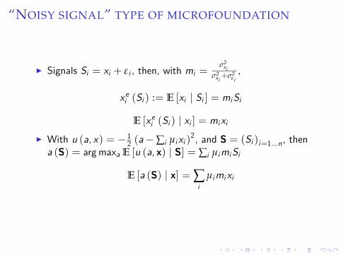
“NOISY SIGNAL” TYPE OF MICROFOUNDATION

I Signals Si = xi + ε i , then, with mi =σ2xi

σ2xi+σ2εi,

xei (Si ) := E [xi | Si ] = miSi

E [xei (Si ) | xi ] = mixiI With u (a, x) = − 12 (a−∑i µixi )

2, and S = (Si )i=1...n, thena (S) = argmaxa E [u (a, x) | S] = ∑i µimiSi

E [a (S) | x] = ∑i

µimixi

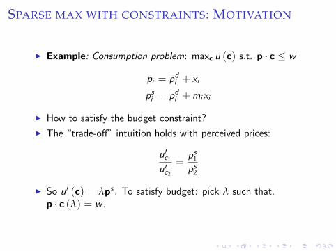
SPARSE MAX WITH CONSTRAINTS: MOTIVATION

I Example: Consumption problem: maxc u (c) s.t. p · c ≤ w

pi = pdi + xi

psi = pdi +mixi

I How to satisfy the budget constraint?I The “trade-off” intuition holds with perceived prices:

u′c1u′c2

=ps1ps2

I So u′ (c) = λps . To satisfy budget: pick λ such that.p · c (λ) = w .

SPARSE MAX WITH CONSTRAINTS

smaxau (a, x) subject to b (a, x) ≥ 0

Define u (a, x ,m) := u (a,m x), b (a, x ,m) := b (a,m x),L (a, x ,m) := u (a, x ,m) + λd · b (a, x ,m), with λd multiplierwhen m = 0.Definition (Sparse max with constraints)Step 1. Allocate attention: with ami := −L−1aa Lami

mi = A(−E [amiLaaami ] /κ)

Step 2: Find action. Solve in a,λ:

ua (a, x ,m∗) + λba (a, x ,m∗) = 0 (perceived model m for FOC)

b (a, x , ι) = 0 (actual model ι for budget)

with ι = (1, ..., 1) =full rationality.

BASIC CONSUMPTION PROBLEM: MARSHALLIAN

DEMANDI I use s for sparse, r for rational / traditional.I Proposition. Demand is:

cs (p,w) = cr(ps ,w ′

)where w ′ solves p · cr (ps ,w ′) = w .

I Quasi-linear utility: Take u (c) = v (c1, ..., cn−1) + cn, with vconcave. Demand for good i < n is independent of wealthand is:

csi (p) = cri (p

s ) .

I If traditional demand is linear in wealth:

cs (p,w) =cr (ps ,w)p · cr (ps , 1)

I Budget is w = $100. I have $105 in my supermarket cart.I Demand linear in wealth: So, I lower my consumption by 5%.I General case: I lower it by −dc = ∂cs

∂w (ps ,w)× $5

SPARSITY MODEL WITH BUDGET CONSTRAINT

I Cobb-Douglas preferences: u (c) = ∑ni=1 αi ln ci ,

csi (p,w) =αipsi

w

∑j αjpjpsj

I CES demand: u (c) = ∑i c1−1/ηi / (1− 1/η)

csi (p,w) = (psi )−η w

∑j pj(psj)−η

CONSUMER AND EQUILIBRIUM THEORY

I From this Marshallian demand, can re-do consumer theory,equilibrium theory

1. Slutsky matrices: non-symmetry, not negative-semi definite2. Expenditure function, Hicksian demand3. Roy’s identity, Shephard’s lemma, WARP4. Nominal illusion5. Producer theory6. Equilibrium theory: Arrow-Debreu, 1st and 2nd welfaretheorems

7. Edgeworth boxes: Phillips curve in each Edgeworth box

I Get a theory of what predictions of basic micro are robust toBR (e.g. sign predictions: “if the price goes up, demand goesdown”), and what are not (like symmetry of Slutsky matrix;absence of nominal illusion).

SPARSE DYNAMIC PROGRAMMINGMOTIVATING EXAMPLE: PERMANENT-INCOME PROBLEM

I max(ct )t≥0 E ∑t βtc1−γt / (1− γ) s.t.:

wt+1 = (1+ r + rt ) (wt − ct ) + y + ytrt+1 = ρr rt + εrt+1, yt+1 = ρy yt + εyt+1

I What’s c (zt ), zt := (wt , rt , yt )?I Want to capture: people “do not think”about the interest rt .I We anchor on the default model:

wt+1 = (1+ r) (wt − ct ) + y

with policy cdt =r wt+yR , value function V d (wt ).

I Call R := 1+ r

SPARSE DYNAMIC PROGRAMMINGMOTIVATING EXAMPLE: PERMANENT-INCOME PROBLEM

I Agent has a “simplifiable subjective model”:

wt+1 = Fw (ct , zt ,m) = (1+ r +mr rt ) (wt − ct ) + y +my ytyt+1 = F y (ct , zt ,m) := ρy (m) yt +mσy εyt+1,

ρy (m) := mρy ρy +(1−mρy

)ρdy

and same for rt+1 as for yt+1: F r := ρr (m) rt +mεr εrt+1,

I The agent allocates attention:

m =(my ,mρy ,mσy ,mr ,mρr ,mσr

)I More generally F z = (Fw ,F r ,F y ), mental model is:

zt+1 = F z (at , zt ,m)

I Often, use

F zi(a, z ,m) = mρi F z

i(a,mi z +

(1−mi

) z i ,d

)+(1−mρi

)z i ,d

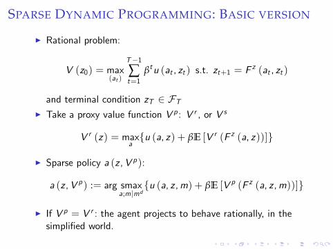
SPARSE DYNAMIC PROGRAMMING: BASIC VERSION

I Rational problem:

V (z0) = max(at )

T−1∑t=1

βtu (at , zt ) s.t. zt+1 = F z (at , zt )

and terminal condition zT ∈ FTI Take a proxy value function V p : V r , or V s

V r (z) = maxau (a, z) + βE [V r (F z (a, z))]

I Sparse policy a (z ,V p):

a (z ,V p) := arg smaxa;m|md

u (a, z ,m) + βE [V p (F z (a, z ,m))]

I If V p = V r : the agent projects to behave rationally, in thesimplified world.

SOME TOOLS

I Proposition: To derive as (w , x) up to second order terms,one can do a Taylor expansion of V d (w) (around the simplemodel), and get the mi . One does not need to solve the fullmodel V r (w , x).

I Proposition: If we have

ar (w , x) = ad (w) +∑ibi (w) xi +O

(‖x‖2

)then the sparse policy is

as (w , x) = ad (w) +∑ibi (w)mixi +O

(‖x‖2

)mi = A

(vaabi (w)

2 σ2xi /κ)

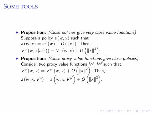
SOME TOOLS

I Proposition: (Close policies give very close value functions)Suppose a policy a (w , x) such thata (w , x) = ad (w) +O (‖x‖). Then,V o (w , x |a (·)) = V r (w , x) +O

(‖x‖2

).

I Proposition: (Close proxy value functions give close policies)Consider two proxy value functions V p ,V p

′such that,

V p (w , x) = V p′(w , x) +O

(‖x‖2

). Then,

a (w , x ,V p) = a(w , x ,V p

′)+O

(‖x‖2

).

SPARSE DYNAMIC PROGRAMMING: OBJECTIVE VALUE

FUNCTION

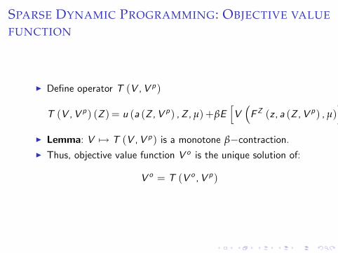
I Define operator T (V ,V p)

T (V ,V p) (Z ) = u (a (Z ,V p) ,Z , µ) +βE[V(FZ (z , a (Z ,V p) , µ)

)]I Lemma: V 7→ T (V ,V p) is a monotone β−contraction.I Thus, objective value function V o is the unique solution of:

V o = T (V o ,V p)

SPARSE DYNAMIC PROGRAMMING: ITERATED

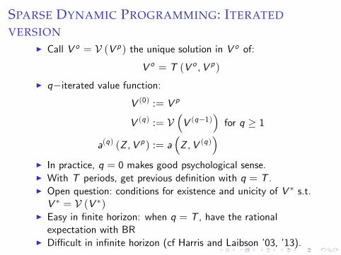
VERSIONI Call V o = V (V p) the unique solution in V o of:

V o = T (V o ,V p)

I q−iterated value function:V (0) := V p

V (q) := V(V (q−1)

)for q ≥ 1

a(q) (Z ,V p) := a(Z ,V (q)

)I In practice, q = 0 makes good psychological sense.I With T periods, get previous definition with q = T .I Open question: conditions for existence and unicity of V ∗ s.t.V ∗ = V (V ∗)

I Easy in finite horizon: when q = T , have the rationalexpectation with BR

I Diffi cult in infinite horizon (cf Harris and Laibson ’03, ’13).

BR PERMANENT INCOME

I Lemma: in the rational policy ct = cdt + ct , with cdt =rwt+yR

c rt = Et

[∑τ≥t

br (wt ) rτ + by yτ

Rτ−t+1

]

br (wt ) :=rR (wt − y)− ψcd

R, by :=

rR

I Proposition: In the sparse model:

cst = Est

[∑τ≥t

br (wt )mr rτ + bymy yτ

Rτ−t+1

]where Es

t is transition function under the subjective model.I AR(1) case:

cs = cd (wt ) + Bsr (wt ) rt + Bsy yt

Bsr (wt ) =br (wt )mrR − ρr (m)

, Bsy =bymy

R − ρy (m)

CALIBRATION

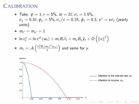
I Take: ψ = 1, r = 5%, w = 2c, σr = 1.5%,σy = 0.3c , φy = 5%, σc/c = 0.15, φr = 0.3, κc = κσc (yearlyunits)

I mr ′ = my ′ = 1

I ln cst = ln cd (wt ) +mrBr rt +myBy yt +O

(‖x‖2

)I mr = A

(σ2r Br (wt )

2 |vcc |κ

)and same for y .

APPLICATION TO LIFECYCLE: FOR THE COMPUTER

I More generally, to solve sparse dynamic programmingI Rational problem:

V (z0) = max(at )t<T

∑0≤t<T

βtu (at , zt ) s.t. zt+1 = F z (at , zt )

1. Decide “default” variables wt in zt = (wt , xt ), u (a, z ,m),F z (a, z ,m)

Use F zi(a, z ,m) = mρi F z

i (a,mi z

)+(1−mρi

)z i ,d

2. Calculate V d (w)3. Calculate some V p (w , x) = V r (w , x) +O

(‖x‖2

)(e.g.

Taylor-expand V (w , x) = V d (w) +∑i Bi (w) xi +O(‖x‖2

)to no need to calculate the whole V r (w , x))

4. Do

a (z ,V p) := arg smaxa;m|md

u (a, z ,m) + βE [V p (F z (a, z ,m))]

5. This way, you can similate the whole policy / life forward.

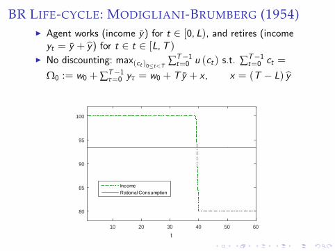
BR LIFE-CYCLE: MODIGLIANI-BRUMBERG (1954)I Agent works (income y) for t ∈ [0, L), and retires (incomeyt = y + y) for t ∈ t ∈ [L,T )

I No discounting: max(ct )0≤t<T ∑T−1t=0 u (ct ) s.t. ∑T−1

t=0 ct =

Ω0 := w0 +∑T−1τ=0 yτ = w0 + Ty + x , x = (T − L) y

t10 20 30 40 50 60

80

85

90

95

100

IncomeRational Consumption

BR LIFE-CYCLE: MODIGLIANI-BRUMBERG (1954)

I Rational agent. Plans ct = Ω0T ,

c0 =w0 + xT

+ y

I Same at future dates t ≤ L

ct =wt + xT − t + y

I Value function:

V r (wt , x , t) = (T − t) u(wt + xT − t + y

)

BR LIFE-CYCLE: BEHAVIORAL

v (ct ,wt , x , t) := u (ct ) + V r (wt + y − ct , x , t + 1)

I Rational agent:

ct = argmaxctv (ct ,wt , x , t)

I Behavioral agent:

ct = arg smaxct ;mt

v (ct ,wt ,mtx , t)

i.e.ct (mt ) =

wt +mtxT − t + y

and evaluated at mt = 0

mt = A(−v tcc

(∂ct∂m

)2|m=0

1κt

)I Calibration: take κt =

∣∣u′′ (cdt )∣∣ κ2.

BR LIFE-CYCLE

t10 20 30 40 50 60

c t

80

85

90

95

100

Consumption

Fully RationalModerately BehavioralVery Behavioral

t10 20 30 40 50 60

wt

0

50

100

150

200

250

Wealth

EVIDENCE

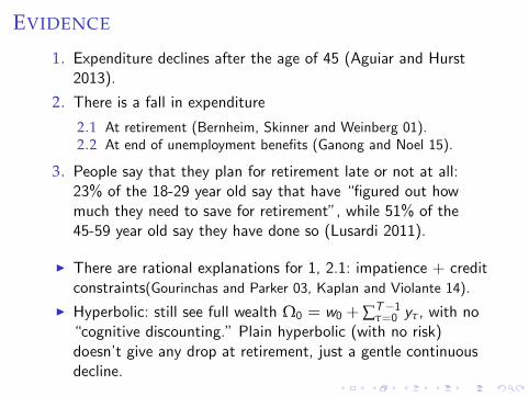
1. Expenditure declines after the age of 45 (Aguiar and Hurst2013).

2. There is a fall in expenditure

2.1 At retirement (Bernheim, Skinner and Weinberg 01).2.2 At end of unemployment benefits (Ganong and Noel 15).

3. People say that they plan for retirement late or not at all:23% of the 18-29 year old say that have “figured out howmuch they need to save for retirement”, while 51% of the45-59 year old say they have done so (Lusardi 2011).

I There are rational explanations for 1, 2.1: impatience + creditconstraints(Gourinchas and Parker 03, Kaplan and Violante 14).

I Hyperbolic: still see full wealth Ω0 = w0 +∑T−1τ=0 yτ, with no

“cognitive discounting.”Plain hyperbolic (with no risk)doesn’t give any drop at retirement, just a gentle continuousdecline.

MORALE FROM LIFECYCLE EXAMPLE

I Sparse agents consume their wealth patiently, like patientrational agents, but are myopic for small things.

I Agents consume wealth w patiently, as a rational agent.I They’re myopic about the future small shocksI The deterministic steady state is rational, it’s the deviationfrom it that’s behavioral

I ...contra models with credit constraints or, hand-to-mouthbehavior.

I The Euler equation fails. The Euler equation holds under theBR-perceived world, but not under the actual world.

I Agents react more to “near” shocks than to “distant” shocks

DEGREES OF FREEDOM AND PSYCHOLOGY

I Psychological considerations determine the “default value”I E.g. in the life-cycle model, ydt = y after retirement: that’s“projection bias”: agents’s default model of the future is thepresent.

I The model does add value:I In lifecycle, generate progressive realization of retirementI Gives a way to handle: self t thinking about self t + 7 thinkingabout self t + 15...

I Likewise, the “frame” is in the basis vector x .I For instance, if the frame is made of nominal prices (plusinflation), the agent will exhibit some nominal illusion

I General rule:I Typically: xdi = E [xi | I ]: replace interest rate by its average...I However what’s the conditioning set I?, e.g. in retirement:ydretirement = E [yt ] = y

A 3-PERIOD MODEL

2

∑t=0u (ct ) .

I Agent receives w0 at time 0, and x at time 2I Will the agent think about x in advance?I Rational: ct = w0+x

3 , c1 = w1+x2 , w1 = w0 − c0

I Proposition:

c0 =w0 +m0x

3, c1 =

w1 +m1x2

, c2 = w2 + x .

with m0 ≤ m1.I m0 = A

( 16κu′′ (w0

3

)σ2x), m1 = A

( 12κu′′ (w1

2

)σ2x).

I People save “too little, too late” for retirement

DERIVATION OF 3-PERIOD PROBLEM: TIMES 2 AND 1I Time 2: V 2 (w2, x) = u (w2 + x)I Time 1: smaxc1;m1 v

1 (c1, x ,m1) with

v1 (c1, x ,m1) = u (c1) + V 2 (w1 − c1,m1x)

c1 =w1 +m1x

2I Attention: ∂m1c1 =

x2 , v

1cc = 2u

′′ (cd1 )m1 = A

(1κv2cc (c)|m1=0 var (∂m1c1)

)= A

(12κu′′(w12

)σ2x

)I Value functions:

V r1 (w1, x) = 2u(w1 + x2

)V RE1 (w1, x) = u(

w1 +m1 (w1) x2

) + u(w1 + (2−m1 (w1)) x

2)

= V r1 (w1, x) +O(x2)

DERIVATION OF 3-PERIOD PROBLEM

I Take V 1,p (w1, x) := V 1,r (w1, x) = 2u(w1+x

2

)=rational

value functionI Time 0: smaxc0;m0 v

0 (c0, x ,m0) with

v0 (c0, x ,m0) := u (c0) + V 1,p (w0 − c0,m0x)

= u (c0) + 2u(w0 − c0 +m0x

2

)

c0 =w0 +m0x

3

m0 = A(1κv0cc |m0=0var (∂m0c0)

)= A

(16κu′′(w03

)σ2x

)

DEVIATIONS FROM RICARDIAN EQUIVALENCE

I Extend previous formula with Tt =government transfer toagent:

cst = by(wt− + Tt

)+ ∑

τ>tmT by

1Rτ−t Tτ

I If the gvt gives T at t, and −RT T in k periods, a BRconsumer increases consumption by

ct = by (1−mT ) T

I A rational consumer wouldn’t change consumption (Barro ’74)I As a result, the government multiplier can easily be greaterthan 1.

I The agents are a mix between Old Keynesian andRicardian-New Keynesian agents.

THE LUCAS CRITIQUE IS LESS POTENT WITH SPARSE

AGENTS

I Lucas: if you change the parameters of the world (e.g. tax),people’s reactions functions will change

I That’s true here for big (or very persistent) deviationsI But it’s not true for small deviations. Then, people keep theirdefault “policy function”.

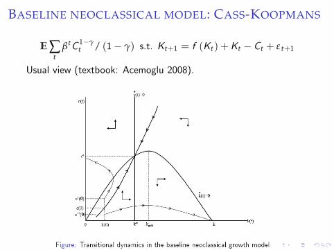
BASELINE NEOCLASSICAL MODEL: CASS-KOOPMANS

E ∑t

βtC 1−γt / (1− γ) s.t. Kt+1 = f (Kt ) +Kt − Ct + εt+1

Usual view (textbook: Acemoglu 2008).

CASS-KOOPMANS: AGENT’S POLICYI Call kt =individual capital, Kt =aggregate.

kt+1 = (1+ r + rt ) kt + y + yt − ctrt = F ′′ (K ∗) Kt , yt = −K ∗F ′′ (K ∗) Kt

I Perceived law of motion:

Kt+1 = (1− φs ) Kt

φs =(1−mφ

)φd +mφφ. Here φd exogenous, or could come

from rational expectations.I Hence policy is, with ξ := u ′(C∗)

u ′′(C∗)F ′′ (K∗) > 0.

ct = r kt +r

r + φsmK yt +

rk∗ − c∗ψr + φs

mK rt

= r kt +ξ

r + φsmK Kt =

(r +

ξmKr + φs

)Kt = (r + φ) Kt

φ = φ0mK , φ0 :=ξ

r + φs

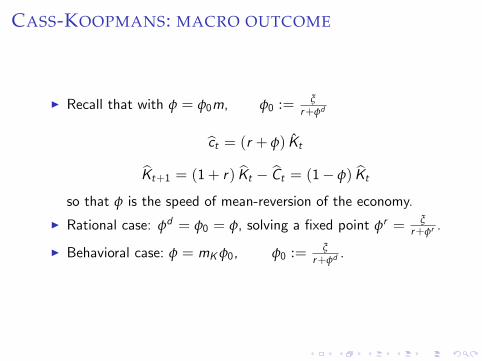
CASS-KOOPMANS: MACRO OUTCOME

I Recall that with φ = φ0m, φ0 := ξr+φd

ct = (r + φ) Kt

Kt+1 = (1+ r) Kt − Ct = (1− φ) Kt

so that φ is the speed of mean-reversion of the economy.

I Rational case: φd = φ0 = φ, solving a fixed point φr = ξr+φr .

I Behavioral case: φ = mKφ0, φ0 := ξr+φd

.

CASS-KOOPMANS: FLUCTUATIONSI Proposition. Suppose that φd ≥ min (φ, φr ). Then

φ ≤ φr

in the sparse economy, GDP fluctuations have slowermean-reversion and higher variance than in the rationaleconomy.

I The speed of mean-reversion of the economy is: φ = φ01+ B

φ0

with φ0 := ξr+φd

, B := 2κ|ucc |σ2ε

. It is lower (and aggregate

fluctuations are larger) when agents’bounded rationality κ isstronger.

I As Kt = (1− φ) Kt−1 + εt , we have

E[K 2t]=

var (εt )

1− (1− φ)2

so low φ means high E[K 2t]

I The speed of mean reversion in the sparse economy will beless than in the rational economy

I With full rat, people should consume more. Then depletes theexcess capital stock, so capital mean-reverts fast.

I With sparsity, there’s a slower depletion of the excess capitalstocks → capital mean-reverts more slowly

I In general: agents have simplifed view of macro dynamics, andact on those

I Quite different from trad. view: “let find the unique path thatdoesn’t lead to an explosion”.

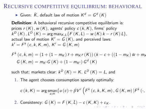
RECURSIVE COMPETITIVE EQUILIBRIUM: BEHAVIORAL

I Given: K , default law of motion K d = G d (K )

Definition: A behavioral recursive competitive equilibrium is:prices r (K ) ,w (K ), agents’policy c (k ,K ), firms’policykD (K ) , LD (K ) = argmaxK ,LF (K , L)− w (K ) k − r (K ) L,actual law of motion K ′ = G (K ), and perceived laws:k ′ = F k (c , k,K ,m), K ′ = G (K ,m)

F k (c, k,m) = (1+ (1−mK ) r +mK r (K )) (k − c + ((1−mK ) w +mKw (K )) L)G (K ,m) = mK ′G (K ) + (1−mK ′)G d (K )

such that: markets clear: kD (K ) = K , LD (K ) = L, and

1. The agent chooses consumption sparsely optimally:

c (k,K ) = arg smaxa;mu (c)+ βV r

(F k (c , k,K ,m) ,G (K ,m) |F k (·,m) ,G (·,m)

)

2. Consistency: G (K ) = F (K , L)− c (K ,K ) + εK .

OTHER APPROACHES

BR in Rep. Determ. Source Bayes Txtbook

static agent actions depdt micro?

contexts allowed attention

Rule-of-thumbs No No Yes Yes No No

Hyperbolics No Yes Yes No Yes No

Credit constraints No No Yes No Yes No

Sticky info. No No Yes Yes Yes No

Noisy info Yes No No Yes Yes No

Entropy penalty Yes No No No Yes No

BGS salience Yes Yes Yes Yes No No

Sparsity Yes Yes Yes Yes No YesNotes: all those models get the higher MPC for current income(except hyperbolic with no credit constraints)Rule-of-thumb consumers: Campbell-Mankiw (1989): a fraction λjust consume current income, ct = yt .Almost all models cannot handleA fortiori, maxa u (a, z) + V (F (a, z))

COMPARISON WITH SIM’S ENTROPY-BASED RATIONAL

INATTENTIONI Very useful, fecund movementI Still, the entropy-based approach is often very complicated

I Cannot (now) do smaxa u (a, x) in closed form, even less

smaxau (a, x) s.t. b (a, x) ≥ 0

I Cannot (now) tractably do

maxc∈Rn

u (c1, ..., cn) s.t.n

∑i=1

pi ci ≤ w .

I A fortiori, dynamic lifecycle is complicatedI The entropy penalty has a nice pedigree, but doesn’t generate(in its strict form) source-dependent inattention

I The sparsity approach is more psychological, a bit more adhoc, very tractable.

I The entropy approach is Bayesian, sparsity explores anon-Bayesian modelling

I Let 1000 flowers bloom

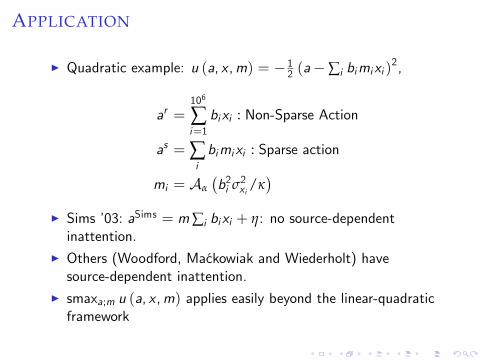
APPLICATION

I Quadratic example: u (a, x ,m) = − 12 (a−∑i bimixi )2,

ar =106

∑i=1bixi : Non-Sparse Action

as = ∑ibimixi : Sparse action

mi = Aα

(b2i σ2xi /κ

)I Sims ’03: aSims = m∑i bixi + η: no source-dependentinattention.

I Others (Woodford, Mackowiak and Wiederholt) havesource-dependent inattention.

I smaxa;m u (a, x ,m) applies easily beyond the linear-quadraticframework

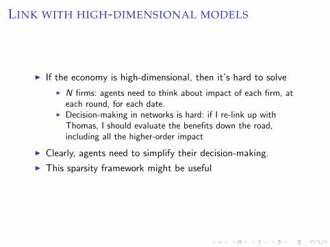
LINK WITH HIGH-DIMENSIONAL MODELS

I If the economy is high-dimensional, then it’s hard to solveI N firms: agents need to think about impact of each firm, ateach round, for each date.

I Decision-making in networks is hard: if I re-link up withThomas, I should evaluate the benefits down the road,including all the higher-order impact

I Clearly, agents need to simplify their decision-making.I This sparsity framework might be useful

POTENTIAL PAYOFFS FOR HIGH-DIMENSIONAL

MODELS

I BR may be useful

1. To model agents who simplify the decision problem (a bit likeKrusell-Smith): for instance, think of just the top 5 firms. Or,the 1st and 2nd round of effect in network effects

2. To analyze the specific impact of bounded rationality.2.1 E.g. perhaps too high (relative) weight on direct impact rather

than indirect impacts? (cf Cohen and Frazzini 08)

I 1. 1.1 over reaction to large firms? e.g. Newspapers spend a lot timetalking about Apple, Walmart...

I It’s hard to have “conscious”decisions (investment...) with inhigh-dimensional economies (but see Carvalho and Grassi(’15) for progress)

I Perhaps this framework will help the development of suchmodels.

CONCLUSION: MICRO BEHAVIOR FOR MACRO

1. Agents react more to near, rather than future, shocks.2. Pervasive failure of the high-frequency Euler equation3. High MPC to tax rebates, especially amongst misoptimizinghouseholds (Parker 15).

4. Agents accumulate a too small buffer of savings, as they’re(partially) myopic to the risk of income fluctuations (Lusardi11)

5. Agents start saving “too late” for retirement (falls at age 45;controversial)

6. Very low sensitivity to interest rates (Hall 88) (so rat IESshould be low). However, people seem OK with non-smoothconsumption profiles (so rat IES should be high).

7. When choosing their portfolio, agents are pay less attention tothe hedging demand motive.

8. Plain introspection: we don’t solve the full macro equilibriumin our head

CONCLUSION: AGGREGATE MACRO

1. Fiscal policy is more powerful, because Ricardian equivalencepartly fails.

2. The Zero Lower Bound is much less costly.3. The Lucas critique has less (or zero) bite4. High fluctuations despite smallish shocks5. The agent is a hybrid of neoclassical agent and old Keynesianagent: partially forward looking.

6. In monetary policy, forward guidance is less powerful.

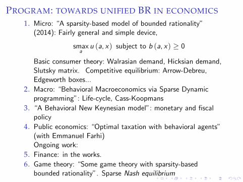
PROGRAM: TOWARDS UNIFIED BR IN ECONOMICS

1. Micro: “A sparsity-based model of bounded rationality”(2014): Fairly general and simple device,

smaxau (a, x) subject to b (a, x) ≥ 0

Basic consumer theory: Walrasian demand, Hicksian demand,Slutsky matrix. Competitive equilibrium: Arrow-Debreu,Edgeworth boxes...

2. Macro: “Behavioral Macroeconomics via Sparse Dynamicprogramming”: Life-cycle, Cass-Koopmans

3. “A Behavioral New Keynesian model”: monetary and fiscalpolicy

4. Public economics: “Optimal taxation with behavioral agents”(with Emmanuel Farhi)Ongoing work:

5. Finance: in the works.6. Game theory: “Some game theory with sparsity-basedbounded rationality”. Sparse Nash equilibrium

CONCLUSION

I Fairly general and simple device, smaxI Prior paper: Gives a behavioral version of the 2 basic chaptersof micro:

I Basic consumer theory: maxc∈Rn u (c) s.t.p · c ≤ w : Marshallian and Hicksian demand, Slutsky matrix,expenditure function, Roy identity...

I Competitive equilibrium theory: Arrow-Debreu, Edgeworthboxes,...

I Here: Sparse dynamic programmingI Applications: Sparse versions of:

I Life-cycle modelI Dynamic macro equilibriumI New Keynesian modelI Basic portfolio choice problem, and hedging demandI Deviations from Ricardian equivalence

I Monetary policy is less powerful; Fiscal policy is morepowerful.