Finance and Economics Discussion SeriesDivisions of Research & Statistics and Monetary Affairs

Federal Reserve Board, Washington, D.C.

Banking Consolidation and Small Firm Financing for Researchand Development

Andrew C. Chang

2016-029

Please cite this paper as:Chang, Andrew C. (2016). “Banking Consolidation and Small Firm Financing for Researchand Development,” Finance and Economics Discussion Series 2016-029. Washington: Boardof Governors of the Federal Reserve System, http://dx.doi.org/10.17016/FEDS.2016.029.

NOTE: Staff working papers in the Finance and Economics Discussion Series (FEDS) are preliminarymaterials circulated to stimulate discussion and critical comment. The analysis and conclusions set forthare those of the authors and do not indicate concurrence by other members of the research staff or theBoard of Governors. References in publications to the Finance and Economics Discussion Series (other thanacknowledgement) should be cleared with the author(s) to protect the tentative character of these papers.

Banking Consolidation and Small Firm Financing for

Research and Development

Andrew C. Chang∗

April 8, 2016

Abstract

This paper examines the effect of increased market concentration of the banking industrycaused by the Riegle-Neal Interstate Banking and Branching Efficiency Act (IBBEA) on theavailability of finance for small firms engaged in research and development (R&D). I measurethe financing decisions of these small firms using a balanced panel of Small Business Innova-tion Research (SBIR) applications. Using difference-in-differences, I find IBBEA decreasedthe supply of finance for small R&D firms. This effect is larger for late adopters of IBBEA,which tended to be states with stronger small banking sectors pre-IBBEA.

JEL Classification Codes: G21, G28, G39, O30Keywords: Banking Deregulation; IBBEA; Interstate Bank Branching Deregulation; Mar-

ket Concentration; Riegle-Neal; Research and Development; R&D; Small Business InnovationResearch; SBIR

∗Board of Governors of the Federal Reserve System. 20th St. NW and Constitution Ave., Washington DC 20551USA. +1 (657) 464-3286. a.christopher.chang@gmail.com. https://sites.google.com/site/andrewchristopherchang/.This research was supported by separate grants from the Department of Economics and the Graduate Division at theUniversity of California - Irvine. However, the opinions expressed in this paper are mine and do not necessarilyreflect those of the university or the Board of Governors of the Federal Reserve System. I thank anonymous referees,Stephanie Aaronson, Volodymyr Bilotkach, Marianne P. Bitler, Nick Bloom, William A. Branch, Jiawei Chen, LindaR. Cohen, Amihai Glazer, Ivan Jeliazkov, David Jenkins, Jakub Kastl, David Neumark, Gary Richardson, George C.Saioc, Matthew Shum, and Don Walls for helpful comments. I also thank Clara C. Asmail, Nicholas Cormier, KayEtzler, and Leslie A. Jensen for help with SBIR data; Daniel J. Wilson for graciously providing state-level data on theuser cost of R&D; and Tyler J. Hanson for valuable research assistance. Any errors are mine.

1

1 Introduction

This paper examines how the deregulation and subsequent consolidation of the U.S. banking in-

dustry affected financing for small firms engaged in research and development (R&D). Because

technological development drives economic growth (Solow, 1957), and because small firms are a

significant driver of innovation (Acs and Audretsch, 1987), understanding the link between small

firm finance and their R&D expenditures is an important issue.

I analyze the effect of the Riegle-Neal Interstate Banking and Branching Efficiency Act of

1994 (IBBEA) on the propensity for small firms to apply for external R&D funding through the

U.S. government’s Small Business Innovation Research (SBIR) program, an award program for

R&D projects at both private and public small firms.1 Prior to IBBEA, there were geographic

restrictions on interstate bank branching, which dated back to the beginning of the U.S. banking

system. Implemented on a state-by-state basis, IBBEA removed geographic restrictions on inter-

state bank branching and consolidated the banking industry. Figure 1, which plots the Herfindahl

Index of the U.S. banking sector from fiscal year (FY) 1987 to FY 2000, shows an increase in

market concentration after IBBEA passed.

With a negative binomial model and difference-in-differences, I estimate the effect of IBBEA

on SBIR applications with a balanced panel of state-year SBIR application counts. I find IBBEA

increased SBIR applications between 10 to 50 percent. This effect is present for all states, but

I find larger effects for states that adopted IBBEA later. Later adopters of IBBEA had stronger

small banking sectors, more potential targets for interstate bank mergers, and the potential to have

a larger change in banking structure due to the deregulation caused by IBBEA (Kroszner and

Strahan, 1999).

The key identification assumption for relating changes in SBIR applications to implications

about small R&D firm finance is that SBIR awards and bank finance are substitutes. Under this

assumption, if IBBEA made it more difficult for firms to secure funding for R&D projects, then

1For a review of U.S. banking deregulation, including IBBEA, see Johnson and Rice (2008). For a summary ofSBIR, see Lerner (1999).

2

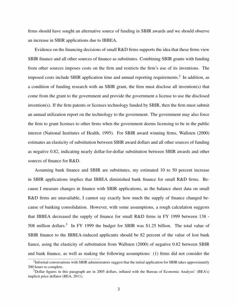
firms should have sought an alternative source of funding in SBIR awards and we should observe

an increase in SBIR applications due to IBBEA.

Evidence on the financing decisions of small R&D firms supports the idea that these firms view

SBIR finance and all other sources of finance as substitutes. Combining SBIR grants with funding

from other sources imposes costs on the firm and restricts the firm’s use of its inventions. The

imposed costs include SBIR application time and annual reporting requirements.2 In addition, as

a condition of funding research with an SBIR grant, the firm must disclose all invention(s) that

come from the grant to the government and provide the government a license to use the disclosed

invention(s). If the firm patents or licenses technology funded by SBIR, then the firm must submit

an annual utilization report on the technology to the government. The government may also force

the firm to grant licenses to other firms when the government deems licensing to be in the public

interest (National Institutes of Health, 1995). For SBIR award winning firms, Wallsten (2000)

estimates an elasticity of substitution between SBIR award dollars and all other sources of funding

as negative 0.82, indicating nearly dollar-for-dollar substitution between SBIR awards and other

sources of finance for R&D.

Assuming bank finance and SBIR are substitutes, my estimated 10 to 50 percent increase

in SBIR applications implies that IBBEA diminished bank finance for small R&D firms. Be-

cause I measure changes in finance with SBIR applications, as the balance sheet data on small

R&D firms are unavailable, I cannot say exactly how much the supply of finance changed be-

cause of banking consolidation. However, with some assumptions, a rough calculation suggests

that IBBEA decreased the supply of finance for small R&D firms in FY 1999 between 138 -

508 million dollars.3 In FY 1999 the budget for SBIR was $1.25 billion. The total value of

SBIR finance to the IBBEA-induced applicants should be 82 percent of the value of lost bank

fiance, using the elasticity of substitution from Wallsten (2000) of negative 0.82 between SBIR

and bank finance, as well as making the following assumptions: (1) firms did not consider the

2Informal conversations with SBIR administrators suggest that the initial application for SBIR takes approximately200 hours to complete.

3Dollar figures in this paragraph are in 2005 dollars, inflated with the Bureau of Economic Analysis’ (BEA’s)implicit price deflator (BEA, 2011).

3

fact that their award chances changed because of banking consolidation and (2) firms that were

induced into applying for SBIR subsequent to IBBEA had an equal expected value of an SBIR

application as a firm that would have applied without IBBEA. Because the estimates indicate that

SBIR applications increased 10 to 50 percent, the lower bound on the change in finance should be

(1− 11+0.1)∗1.25 billion = 0.82∗bank f inance lowerbound, or 1

0.82 ∗ (1−1

1+0.1)∗1.25 billion =

138 million = bank f inance lowerbound. A similar calculation for the upper bound is 10.82 ∗ (1−

11+0.5)∗1.25 billion = 508 million = bank f inance upperbound.

My panel of state-year SBIR application counts is a data set that offers three advantages for

this study. First, because the data set comes from administrative records, it is free of the self-

reporting bias present in survey data.4 Second, the data set is a balanced panel of SBIR application

counts that is free of the survivorship bias usually present in bank or firm-level data. Third, the

panel of SBIR application counts represents both public and private companies as opposed to just

public companies (for example, companies in Compustat). This last advantage allows an analysis

of small private companies, which are important to the conduct of R&D and for which little data

are available. Previous research on banking deregulation looks at the effect of deregulation on the

average small firm or the effect on lending for small firms at the state level, finding mixed results

on how deregulation affected the supply of credit (Jayaratne and Wolken, 1999; Vera and Onji,

2010). To my knowledge, this paper is the first that examines the effects of IBBEA specifically on

small, private R&D firms.

2 Institutional Details of IBBEA and SBIR

This section reviews IBBEA and SBIR. I discuss how IBBEA led to the consolidation of the bank-

ing industry. For SBIR, I describe how the program is structured and present summary statistics of

small R&D firms that are eligible for SBIR.

4See, for example, Berger and Udell (1995) and Peek and Rosengren (1996) for evidence of errors in survey data.

4

2.1 IBBEA

Passed on September 29, 1994, IBBEA set a default opt-in trigger date of June 1, 1997. However,

states could opt into IBBEA early or opt out of IBBEA entirely by the default opt-in date. Approx-

imately one-third of states waited until the trigger date to opt into IBBEA’s provisions, and several

states had active debates on opting out of IBBEA (Kane, 1996; Johnson and Rice, 2008). Texas

and Montana initially opted out, although both states later opted in. Table 1 shows the initial opt-in

dates for each state. Subject to certain conditions, IBBEA allowed several new types of banking

activity: (1) interstate bank acquisitions, (2) interstate agency operations, (3) interstate branching,

and (4) de novo branching (Johnson and Rice, 2008).

IBBEA changed the structure of the banking industry. Prior to IBBEA, in 1994 there were

only 62 out-of-state bank branches — less than 1 percent of the total number of branches. With the

removal of the restrictions on interstate branching, by 1999 there were more than 10,000 out-of-

state bank branches — approximately 20 percent of the total number of bank branches (Johnson

and Rice, 2008).

In addition to allowing interstate bank branches, IBBEA increased interstate bank mergers,

which contributed to the consolidation of the banking industry documented in Figure 1. Figure

2 plots interstate bank mergers during the 1990s and shows a significant increase in interstate

mergers subsequent to IBBEA.

IBBEA fueled research on the relationship between banking consolidation, deregulation, and

finance.5 This research may have been encouraged by suspicions that IBBEA was detrimental for

small firm finance, which was also a chief concern in Congress when IBBEA was debated (U.S.

Congress, 1993).

5Examples include Berger, Saunders, Scalise, and Udell (1998); Cole and Walraven (1998); Peek and Rosengren(1998); Strahan and Weston (1998); Jayaratne and Wolken (1999); Craig and Hardee (2007); Rice and Strahan (2010);Vera and Onji (2010); and Cornaggia, Mao, Tian, and Wolfe (2015).

5

2.2 SBIR

Congress created the SBIR program in 1982 in part to combat market failures associated with

R&D.6 Public Laws 97-219, 99-443, and 102-564 require each federal agency with an extramural

research program greater than $100 million to set aside a fixed percentage of the agency’s ex-

tramural research budget for SBIR. Certain characteristics of the SBIR program are mandatory

(for example, the set-aside percentage), and the Small Business Administration (SBA) oversees

the general SBIR program. However, each agency administers its own SBIR program separately,

which gives the individual agencies some flexibility to meet SBIR’s congressional mandates.7

Qualified businesses that can receive an SBIR award are located in the U.S., are for-profit, are

at least 51 percent owned by U.S. citizens or permanent residents, and employ a maximum of 500

employees. Financial data on firms that applied for SBIR are not available. However, the 1993

National Survey of Small Business Finances (NSSBF) contains financial and other demographic

data on small firms that employed R&D workers, which are the types of firms that would have

applied for SBIR grants (Board of Governors of the Federal Reserve System, 1993).8 Most of the

survey describes characteristics of firms in 1993, although some questions reference either 1992 or

1994.

Table 2 displays characteristics of firms that employed R&D workers from the 1993 NSSBF.

Column (1) describes all firms that employed R&D workers in 1992. Column (2) restricts the

sample to only firms with R&D workers in 1992 that also applied for venture capital from 1992 to

1994. The table inflates all dollar figures to 2005 dollars with the BEA’s implicit price deflator.

Column (1) shows that in 1992, the average small R&D firm had 12 workers, almost a quarter

million dollars in payroll, and more than $1.6 million in sales. Importantly for this paper, 38.9

6For market failures, in addition to the liquidity constraint problem arising from uncertainty and asymmetric infor-mation (Arrow, 1962; Hall and Lerner, 2009), R&D also suffers from an appropriation issue (Griliches, 1992).

7As of FY 1999, the participating agencies were the Departments of Agriculture, Commerce, Defense, Educa-tion, Energy, Health and Human Services, and Transportation; the Environmental Protection Agency; the NationalAeronautics and Space Administration; and the National Science Foundation.

8The NSSBF defines a small firm as one with fewer than 500 employees, which is the same definition that SBIRuses. The NSSBF has data available for 1987, 1993, 1998, and 2003. However, the 1998 edition did not collectinformation on R&D employees, and the 1987 and 2003 editions are outside of this paper’s sample period.

6

percent of these firms applied for a loan from 1993 to 1994 and, on average, were approved for

more than half a million dollars. These data show that loans are an important source of finance for

these firms. Firms that also applied for venture capital were larger, on average, than those that did

not. In addition, firms that applied for venture capital also secured loans as a source of finance.

Agencies divide their SBIR awards into either two or three phases. A Phase I award is for a firm

to explore the technical and commercial feasibility of the R&D project. If the results of the Phase

I project are promising, the firm may be invited to apply for a Phase II award to further develop

and commercialize the idea. Firms cannot undertake a Phase II project without first completing

Phase I. Some agencies also have a Phase III program, which involves partnering the firm with a

collaborator; this phase does not provide additional government SBIR money.

For the empirical analysis, I use the total state by FY SBIR Phase I applications for the agencies

with the largest SBIR budgets: the Departments of Defense, Energy, and Heath and Human Ser-

vices; the National Aviation and Space Administration (NASA); and the National Science Foun-

dation (NSF). These five agencies compose more than 96 percent of the SBIR budget in each FY

(National Science Board, 2008). I use Phase I applications as the dependent variable because these

give the strongest indicator of the effort small R&D firms expend to seek external finance.9 Phase

II and Phase III applications represent a mixture of firm effort and agency politics, as they are

conditional on good progress in earlier SBIR phase(s) and can require an invitation by the SBIR

agency to even apply.

3 Model and Data

3.1 Model

Two features of IBBEA’s deregulation are important for this study. First, the removal of banking

restrictions consolidated the banking industry and potentially affected the cost of credit (Cole and

Walraven, 1998; Peek and Rosengren, 1998; Strahan and Weston, 1998; Jayaratne and Wolken,

9Unfortunately, I do not observe the total dollar amount applied for, only the application count.

7

1999; Craig and Hardee, 2007; Rice and Strahan, 2010; Vera and Onji, 2010). Second, because

there is between-state variation in deregulation dates, I can identify the effect of IBBEA on small

R&D firm finance in a treatment-control setup.

Because the dependent variable, SBIR applications, is a count variable, I estimate a negative

binomial model (Cameron and Trivedi, 1998, 2005). The negative binomial model is

f (yi,t |λi,t) =exp(−λi,t)λ

yi,ti,t

yi,t!, λi,t = µi,tν (1)

where

µi,t = exp(X ′i,tβ ) (2)

νiid∼ g(ν |α) (3)

E(yi,t |µ,α) = µi,t (4)

Var(yi,t |µi,t ,α) = µi,t +αµ2i,t (5)

In equations (1) to (5), i is a state, t is the FY, exp(•) is the exponential function, E(•) is

the expectations operator, Var(•) is the variance, X is a matrix of covariates, and α, β and δ are

parameters to be estimated.

In addition to the fact that the negative binomial model only predicts non-negative outcomes,

the negative binomial model’s estimated marginal effects account for heterogeneous state sizes.

Differentiating the conditional mean in equation (4) with respect to a single covariate x j, the ex-

pected marginal effect for y with respect to x j is

dE(y| X)

dx j= β j× exp(X ′β ) (6)

8

which depends on the parameter for covariate x j, β j, the entire matrix of covariates X , and their

associated parameters β through the term exp(X ′β ).10

3.2 Policy Variable

A standard policy variable is an indicator for post-deregulation that assumes a uniform effect of

deregulation over time. I instead construct the policy variable to allow for time-varying effects of

deregulation.

I divide states into three cohorts, one for each FY from the passage of IBBEA to the IBBEA

trigger date: (1) deregulators by FY 1995, (2) deregulators in FY 1996, and (3) deregulators in FY

1997. For each cohort, I model the policy implementation as a series of time dummies beginning

in the year immediately after the cohort passes IBBEA.11 For example, for the earliest deregulation

cohort (by FY 1995), there are four time dummies: FY 1996, FY 1997, FY 1998, and FY 1999.

For the FY 1996 deregulators, there are three dummies: FY 1997, FY 1998, and FY 1999. The

same pattern holds for the last cohort. This type of policy variable allows heterogeneous effects of

IBBEA by deregulation cohort as well as through time.

Formally, let Dt be a year dummy for FY t and Di,τ be a dummy for state i if it deregulated in

FY τ . The conditional mean for state i in FY t with the policy variable is:

µi,t = exp(1999

∑t=1996

ζtDtDi,1995 +1999

∑t=1997

ηtDtDi,1996 +1999

∑t=1998

θtDtDi,1997 +X ′i,tβ ) (7)

In equation (7), ζt represents the effect of IBBEA on SBIR applications in FY t for the group

of states that deregulated by FY 1995, ηt represents the effect of IBBEA on SBIR applications in

FY t for the group of states that deregulated in FY 1996, and θt represents the effect of IBBEA on

SBIR applications in FY t for the group of states that deregulated in FY 1997.

I model the policy variable using equation (7) instead of the standard policy indicator vari-

able to be completely flexible for allowing time-varying effects of IBBEA by deregulation cohort.

10Tests for overdispersion consistently reject H0 : α = 0. vs. HA : α 6= 0.11Section 5 considers alternate timings of the policy variable that produce similar results.

9

There are at least three reasons to expect that IBBEA had different effects both over time and by

deregulation cohort. One reason is that when states deregulated, it affected the banking industry

in states that had already deregulated. For example, when states deregulated in 1995, banks could

conduct interstate mergers but only between banks in the deregulated states. When the next wave

of states deregulated in 1996, the banks in these states could merge with other banks in the newly

deregulated states and also with banks in states that were already deregulated. Similarly, states that

were already deregulated had a new influx of banks with which they could merge. Therefore, each

new wave of deregulation affected the banking industry in both the newly deregulated states and

the states that had already deregulated, which implies that IBBEA had time-varying effects and

makes the standard indicator policy variable unsatisfactory.

A second reason to expect different effects of IBBEA by deregulation cohort is that later

adopters of IBBEA had stronger small banking sectors than early adopters (Kroszner and Stra-

han, 1999). Therefore, for later adopters there was a potential for a greater amount of change

post-IBBEA.

A third reason is a timing and learning story. Suppose that when the first wave of deregula-

tion passed in 1995, banks were unfamiliar with the procedures needed to instigate the now-legal

mergers. Therefore, some banks in the states that deregulated in 1995 may have delayed merging.

However, by 1997, banks may have been familiar with these procedural hurdles and could execute

mergers more quickly than when IBBEA was first passed. In this scenario, we can expect the effect

of deregulation on market concentration to vary over time. I model IBBEA’s time-varying effect

as the flexible form in equation (7) to be completely agnostic on the mechanism behind changes in

banking concentration.12

12An even more flexible policy variable would be able to take into account the degree of deregulation, as stateshad some latitude to restrict interstate branching (Johnson and Rice, 2008). However, there is not a clear way toparametrize the dimensions to which states were allowed to deregulate. As a robustness check, I create an alternatepolicy variable that takes into account the restrictions on interstate branching based on the indicator from Rice andStrahan (2010) with the same time-series form as equation (7). This alternate policy variable indicates that SBIRapplications increased between 7 to 15 percent by FY 1999, calculated for the mean deregulator, but the estimatesare less precise (significant at the 10 percent level to insignificant), which suggests that the dimensions by whichstates were allowed to restrict interstate branching might not be important factors in determining the effect of bankingconsolidation on SBIR applications.

10

3.3 Dependent Variable and Controls

The dependent variable is state-FY SBIR Phase I applications that come from a balanced panel

from FY 1990 to FY 1999. SBIR programs at participating federal agencies are independently

operated and funded. I aggregate SBIR applications from the five largest SBIR agencies to create

the panel: the Departments of Defense, Energy, and Health and Human Services - National Insti-

tutes of Health; NASA; and the NSF. The SBIR programs for these five agencies compose more

than 96 percent of the budget for SBIR in each FY (National Science Board, 2008). For NASA,

the data are available on NASA’s website (National Aviation and Space Administration, 2010).

For the remaining agencies, I query the relevant SBIR officials to obtain the data sets.13 Except

for the applications from Hawaii in FY 1993 and North Dakota in FY 1994 to the Department of

Defense, the data set contains data for all five agencies in each state and FY. The results are robust

to excluding Hawaii and North Dakota.

The key identification assumption relating changes in SBIR applications caused by IBBEA

to IBBEA’s effect on small R&D firm finance is that SBIR applications and bank finance are

substitutes (Wallsten, 2000). Therefore, if we observe an increase in SBIR applications, then the

implication is that IBBEA decreased the supply of bank finance. In this situation, firms switched

from bank finance to trying to receive an SBIR award, which increased SBIR applications. The

opposite holds for a decrease in SBIR applications.

To identify the effect of IBBEA on SBIR application rates, I use a variety of additional covari-

ates that control for other factors that can influence a state’s SBIR applications. I use state fixed

effects to remove time-invariant characteristics of states that could affect SBIR applications. I also

include state-specific time trends and time dummies to control for the trend of SBIR applications

prior to IBBEA.

I remove the effects of the business cycle on SBIR applications using gross state product from

the BEA (BEA, 2011). R&D expenditures are correlated with the business cycle, which implies

13Specifically, I use the Freedom of Information Act (Department of Defense, 2010; Department of Energy, 2010;National Science Foundation, 2010a; National Institutes of Health, 2010).

11

that the financing patterns for R&D, including SBIR applications, should also be correlated with

the business cycle regardless of the state of banking deregulation (Barlevy, 2007; Chang, 2013).

Changes in the number of SBIR applicants may be affected by changing demand for the funds

for SBIR, as opposed to the supply-side effects this paper investigates. For example, if the number

of small electronics firms in a state increases, then the number of SBIR applications to agencies that

fund R&D projects in electronics should also increase. Because firms that receive SBIR awards

are primarily from the North American Industry Classification System (NAICS) industry R&D in

the Physical Sciences (NAICS 541710), to control for the universe of potential applicants I add the

number of employees and the total establishment count of firms in R&D in the Physical Sciences

into the regressions.14,15 Total employee counts by state, six-digit NAICS industry, and FY come

from the Bureau of Labor Statistics’ Quarterly Census of Employment and Wages (QCEW) (BLS,

2011). I also estimate specifications with total employment and establishment counts in the top-10

six-digit NAICS codes that give similar results.16

The propensity for a firm to seek funding may also be a function of other state-specific fac-

tors. For example, if a state adopts policies that are more friendly to innovative activities, then it

could alter the SBIR application rate for that state. Alternatively, through the fertile technology

hypothesis, if a large amount of innovation occurs in a particular state, then it can create additional

14To determine the industry composition of SBIR-award-winning firms, I use data on SBIR award winners fromthe SBA’s TECH-Net database (SBA, 2010). The database records details on SBIR awards: characteristics of winningfirms, the abstracts of the SBIR proposals, amount of the award, etc. I take a random sample of 1000 SBIR awardsfrom FY 1990 to FY 2000, divided evenly over each of the five largest SBIR agencies by budget, and use TECH-Net’s information to assign each award-winning firm to either one or two NAICS codes. I match the sampled firmsfrom TECH-Net to publicly available databases that contain information on firms and their product lines (Dun andBradstreet, 2010; Federal Government Bid Intelligence Company, 2011; Gale Group, 2010) as well as crosscheck theinformation from these databases against available public reports, company websites, published articles, and patentapplications to accurately assign the SBIR awardees to NAICS codes.

15For this control to be valid, the industry distribution of the SBIR-award-winning firms needs to be similar to theindustry distribution of all SBIR applicants. Although there are no data available to analyze this relationship directly,the most common industry classification for all SBIR applicants is likely R&D in the Physical Sciences (NAICS541710). SBIR agencies typically solicit proposals for technologies to fulfill a specific agency research requirement,and there is no reason to suspect applicants from outside R&D-intensive industries would apply for SBIR awards.

16The other top NAICS codes are: 325414 (biological product, excluding diagnostic, manufacturing), 334413 (semi-conductor and related device manufacturing), 334511 (search, detection, navigation, guidance, aeronautical, and nau-tical system and instrument manufacturing), 339112 (surgical and medical instrument manufacturing), 541330 (engi-neering services), 541380 (testing laboratories), 541511 (custom computer programming services), 541512 (computersystem design services), and 541690 (other scientific and technical consulting services).

12

opportunities for innovative activities, which would alter the SBIR application rate through a chan-

nel other than IBBEA (Kortum and Lerner, 1998). I add three controls to the model to proxy for

the innovative climate in a state.

First, I add total state academic R&D expenditures. Academic R&D expenditures should be

correlated with the degree of innovative atmosphere in a state, particularly where basic research

is concerned. Data on academic R&D expenditures come from the NSF’s WebCASPAR database

National Science Foundation (2010b). Second, I use Wilson (2009)’s estimate of the state-level

cost of R&D capital, which is a function of a state’s corporate tax and R&D tax policies. A change

in the cost of R&D should induce firms to change their R&D project portfolio and therefore affect

their demand for R&D financing.17 Third, I use utility patent applications, conditional on eventual

patent approval.18 Although noisy, patent counts offer one measurement of the amount of inventive

activity in a state. Data on utility patents come from the National Bureau of Economic Research

(NBER) patent database, documented in Hall, Jaffe, and Trajtenberg (2001) and available from

NBER (2011).

Firms may also decide to apply for SBIR as a function of agency-specific investment in the

state. For example, suppose the Department of Defense increases its R&D funding in Alabama.

Firms in Alabama would then begin to acquire knowledge of and familiarity with the Department

of Defense’s technological and R&D demands. This familiarity could induce firms in the state to

apply for SBIR awards, as they would have garnered additional information on the department or

have revised estimates of the expected value of an SBIR award. To control for agency-specific

investment, I add total R&D obligations for U.S. performers by the five SBIR agencies into the

model. Data on R&D obligations come from the NSF’s WebCASPAR database (?).

17Other examples of research into R&D tax incentives include Chang (2014) and Guceri and Liu (2015).18To determine which types of patents to include in this measure, I sample the largest SBIR agency’s (Department

of Defense) award winners from the SBA Tech-Net Database. I present results where the patent count control variableincludes total patent applications for the following two-digit Hall, Jaffe, and Trajtenberg (2001) technology categories:gas (13), communications (21), computer hardware and software (22), computer peripherals (23), information stor-age (24), electrical devices (41), electrical lighting (42), measuring and testing (43), nuclear and x-rays (44), powersystems (45), semiconductor devices (46), miscellaneous electronics (49), materials processing and handling (51),metalworking (52), motors (53), optics (54), transportation (55), miscellaneous mechanical (59), and heating (66). Ialso check the results using all patent applications, and the results are nearly identical.

13

Table 3 displays summary statistics of the dependent variable and controls.19

4 Results

Table 4 presents the estimated average marginal effects from the baseline model.20 Column (1)

presents a parsimonious specification with only aggregate time dummies, state time trends, and

state fixed effects. The marginal effects reported indicate the average change in SBIR applications

by cohort for each FY subsequent to deregulation relative to the pre-IBBEA period. Column (2)

presents the same specification as column (1) in percent changes. For example, in the first row

of results, for the states that deregulated by FY 1995, column (1) estimates deregulation to have

an average effect of increasing SBIR applications by 35.8 per state in the FY immediately after

deregulation. From the same row in column (2), this average marginal effect translates to a 6.71

percent increase over the pre-IBBEA period. Adding additional state controls in column (3) yields

similar effects for all IBBEA cohorts. Column (4) displays the results of column (3) in percent

terms.21

From Table 4, for almost all treatment periods, the model indicates that IBBEA increased

SBIR applications. Under the assumption of constant substitutability between bank finance and

SBIR awards, this increase in applications implies IBBEA decreased the supply of bank finance

for small R&D firms. In addition, for all cohorts this decrease in finance is exacerbated over time.

For the FY 1995 cohort, immediately after deregulation (FY 1996) there is a small effect (6.71

percent) of IBBEA on SBIR applications. However, the estimates for four years after deregula-

tion (FY 1999) indicate a 25.2 percent increase in SBIR applications. A similar upward trend

in applications holds for the FY 1996 and FY 1997 cohorts, implying a downward trend in the

19I also experiment with specifications that include the state-level unemployment rate and the state-level unemploy-ment rate interacted with the fed funds rate, which is a covariate that could capture heterogeneous effects of monetarypolicy on SBIR applications. These specifications give similar results, and I omit them for brevity.

20For state i’s regressor j, xi, j, the average marginal effect is 1N ∑

Ni=1

dyidxi, j

, where N is the total number of states.21Removing the time effects generates estimates close to zero for all cohort years. The time dummies and state time

trends account for the pre-IBBEA trend in SBIR applications.

14

supply of finance.22 For the FY 1995 and FY 1996 cohorts, the effect of IBBEA on SBIR appli-

cations is statistically significant at the 5 percent level in 1999; for the FY 1997 cohort the effect

is significant in 1998. Late adopters of IBBEA had stronger small banking sectors, more possible

targets for interstate bank mergers, and the potential to have a larger change in banking structure

subsequent to deregulation (Kroszner and Strahan, 1999). One possible explanation for the up-

ward trend in SBIR applications is the successive waves of consolidation caused by IBBEA, which

caused steadily increasing market concentration.

Of the control variables in Table 4, patent counts and agency R&D obligations are individually

significant, and the joint F-test of all control variables indicates the controls are jointly significant.

In unreported specifications that include additional lags of the control variables or differences of

the controls, the effect of IBBEA on SBIR applications is similar to the baseline.23

The tendency for SBIR applications to rise from FY 1997 to FY 1999 corresponds with the

large increase in market concentration of the commercial banking sector, suggesting the increased

concentration of the banking industry decreased small firm finance for R&D. The estimation is

consistent with the hypothesis that the relationship lending channel of small banks is more impor-

tant than the geographic diversification potential of large banks for small R&D firm financing.24

5 Robustness Checks

In this section, I present additional robustness checks on the main results from section 4.

22Weighting states by gross state product still shows an upward trend in applications for all cohorts. The weightedestimates are similar to the unweighted estimates for the FY 1995 and FY 1996 cohorts. For the FY 1997 cohort,the weighted estimates are about half of the unweighted estimates. For all cohorts, the coefficients for IBBEA arestatistically significant at standard levels.

23To check for stationarity of covariates, I run the Harris and Tzavalis (1999) small-T adjusted panel unit root test.The test indicates that academic R&D, the user cost of R&D, patent count, gross state product, and the establishmentcount are non-stationary. To address the potential effect of non-stationary covariates on my results, I conduct twoexercises: (1) I reestimate the model with only the stationary covariates from the baseline specification, and (2) I first-difference the non-stationary covariates and reestimate the model with these differenced covariates (the Harris andTzavalis (1999) test indicates that all of the first-differenced covariates are stationary). In both of these specifications,the estimates of the effect of IBBEA on SBIR applications are similar to the baseline, with IBBEA increasing SBIRapplications by 22 to 36 percent, depending on the deregulation cohort.

24Evidence on the causes and consequences of relationship lending is mixed. See, for example, Elsas (2005),Presbitero and Zazzaro (2011), and Mudd (2013).

15

5.1 Policy Variable Timing

The first robustness check I consider is the timing of the policy variable. The policy variable

in section 4 models IBBEA as taking effect the year after deregulation. However, banks could

potentially respond to deregulation either faster or slower than with a one year lag. Therefore, I

adjust the timing of the policy variable to start either in the year IBBEA was passed or two years

after, as opposed to one year after.

Table 5 shows the results for changing the timing of the policy variable. Columns (1) and (2)

show the results of modeling IBBEA as having an effect the year it was passed. Columns (3)

and (4) model IBBEA’s effect as two years after it was passed. Columns (1) and (3) report the

average marginal effect in levels, and columns (2) and (4) report the effects of columns (1) and (3)

in percents.25

The treatment patterns when shifting the timing of the policy variable in Table 5 are similar to

the baseline model in Table 4. From columns (1) and (2) of Table 5, modeling the treatment as

having an effect the year IBBEA was passed still suggests that IBBEA increased SBIR applications

and therefore decreased the supply of finance for small R&D firms. As with the baseline model,

there is an upward trend in SBIR applications. From column (2) of Table 5, for the FY 1995

deregulation cohort there is a mere 2.95 percent increase in SBIR applications in FY 1995, but

this number grows monotonically to 41.5 percent by FY 1999. The same upward patterns of SBIR

applications hold for the other two deregulation cohorts.

Changing the treatment to have an effect two years after deregulation (columns 3 and 4) at-

tenuates the estimated increases in SBIR applications, but the point estimates are generally still

positive and increase with time as in the previous specifications. In FY 1999, relative to the base-

line (Table 4, column 4), the estimated increase in SBIR applications due to IBBEA disappears for

the FY 1995 cohort, changes from a 30.5 percent increase to a 17.4 percent increase for the FY

1996 cohort, and changes from a 37.7 percent increase to a 23.1 percent increase for the FY 1997

25Table 5 does not report the control variables to save space, but the signs and magnitudes of the control variablesare similar to the baseline in Table 4. The F-test for significance of all controls is significant for at least the 5 percentlevel.

16

cohort.

5.2 Specific States

An additional concern is whether certain states drive the results in Table 4. Specifically, I consider

North Dakota (ND), Montana (MT), and Texas (TX) by individually excluding each of these states

from the estimation. Table 6 shows the results. Column (1) presents the baseline results (Table 4,

column 4) for comparison.

The Bank of North Dakota anchors North Dakota’s banking system as the only state-owned

bank in the United States. State law tasks the bank with “promot[ing] agriculture, commerce, and

industry in North Dakota” (Bank of North Dakota, 2011). Because of the presence of a state-

owned bank, the effect of IBBEA on North Dakota could have been different from the average

effect across states. Therefore, I re-estimate Table 4 without North Dakota, which yields similar

results as shown in Table 6, column (2).

Next, I turn my attention to the control group, which varies over time. For example, in FY

1995, identification of the effect of IBBEA uses states that deregulated later than FY 1995 as a

control group. In FY 1996, the model identifies the effect of IBBEA on deregulators in FY 1995

and FY 1996 using the control group of all states that deregulated later than FY 1996. Finally,

identifying the effect of IBBEA in FY 1997 to FY 1999 for deregulators from FY 1995 to FY 1997

uses the two states that opted out of IBBEA, Montana and Texas, as a control group. Identification

of the parameters in all regressions requires the control group to be unaffected by region-specific

shocks. Because Montana and Texas are in the control group for the entire time period, and the

model identifies the effect of IBBEA from FY 1997 to FY 1999 using these two states as a control

group, I check to see whether a state-specific shock to either Montana or Texas drives the results.

To do so, I individually exclude Montana and Texas from the estimation. If, for example,

Montana experienced a shock to SBIR applications but Texas did not, then the estimates using just

Montana as a control group should be different than when using just Texas as a control group and

both estimates should be different than when using both states as a control group, as in Table 4.

17

Similarly, I can rule out a state-specific shock driving the results when the estimates using either

Montana or Texas or both Montana and Texas are all similar.

When sequentially excluding the control states, the results are similar to using both control

states. IBBEA continues to increase SBIR applications and decrease the supply of finance for

small R&D firms. Using just Texas as a control state in column (4) generates larger estimates of

this effect than either using both Montana and Texas or just Montana, but all of the qualitative

results from the baseline model continue to hold.

6 Conclusion

The deregulation of interstate bank branching and relaxed restrictions on interstate bank mergers by

IBBEA increased market concentration in the U.S. banking industry. This paper uses a balanced

panel to investigate how the increase in market concentration by IBBEA affected the supply of

finance for small R&D firms. The applicants to SBIR are small R&D firms, both private and

public.

Economic theory gives an ambiguous prediction of the effect of banking consolidation on small

firm financing. Large banks benefit from geographic diversification. Because large banks are

involved in multiple, geographically distinct product markets, they are able to distribute risk over

different regions and shield themselves against adverse regional capital or business shocks (Peek

and Rosengren, 1996). The diversification potential of large banks gives them an advantage over

small banks when offering financing terms for small R&D firms.

However, when trying to obtain a source of finance, the firm will generally have superior in-

formation about the value of the firm relative to a prospective financier. This information disparity

is particularly true of small R&D firms, which have little collateral or other hard information to

signal their worth to financiers. Small banks, by forming long-term relationships with and collect-

ing soft information on clients (for example, a firm owner’s work ethic), can reduce informational

asymmetries and therefore offer superior financing terms to large banks, which rely on transaction

18

lending (for example, credit histories) to make investment decisions (Petersen and Rajan, 1994;

Stein, 2002).

I find that IBBEA decreased the supply of finance for small R&D firms. This result implies

that the relationship lending channel of small banks, in which small banks develop long-term

relationships with potential clients to overcome information asymmetries associated with finance,

might be more important than the geographic diversity advantage of large banks for small R&D

firm finance (Petersen and Rajan, 1994; Peek and Rosengren, 1996).

Government support for R&D is justified by the presence of market failures for R&D. These

market failures stem from at least two characteristics of R&D: (1) the social return to R&D is

higher than the private return to R&D, as innovators are unable to capture profits from the positive

spillovers associated with their inventions (Griliches, 1992; Samuelson, 1954), and (2) asymmetric

information between firms and potential financiers complicates the financing of R&D and gives

rise to market failures due to moral hazard and adverse selection problems (Arrow, 1962). This

paper suggests banking consolidation worsened these market failures.

References

Acs, Zoltan J., and David B. Audretsch, “Innovation, Market Structure, and Firm Size,” Review of

Economics and Statistics 69:4 (1987), 567-574.

Arrow, Kenneth J., “Economic Welfare and the Allocation of Resources for Invention” (pp. 609-

626), in Richard R. Nelson (Ed.), The Rate and Direction of Inventive Activity: Economic and

Social Factors (Princeton: Princeton University Press, 1962).

Bank of North Dakota, Bank of North Dakota. http://www.banknd.nd.gov/. Accessed March 10,

2011.

19

Barlevy, Gadi, “On the Cyclicality of Research and Development,” American Economic Review

97:4 (2007), 1131-1164.

Berger, Allen N., Anthony Saunders, Joseph M. Scalise, and Gregory F. Udell, “The Effects of

Bank Mergers and Acquisitions on Small Business Lending,” Journal of Financial Economics

50:2 (1998), 187-229.

Berger, Allen N., and Gregory F. Udell, “Universal Banking and the Future of Small Business

Lending,” New York University Working Paper FIN-95-009 (1995).

Bureau of Economic Analysis (BEA), Regional Economic Accounts.

http://www.bea.gov/regional/gsp/action.cfm. Accessed February 7, 2011.

Bureau of Labor Statistics (BLS), Quarterly Census of Employment and Wages.

http://www.bls.gov/cew/. Accessed February 12, 2011.

Board of Governors of the Federal Reserve System, 1993 National Survey of Small Business

Finances. http://www.federalreserve.gov/pubs/oss/oss3/nssbf93/nssbf93home.html#nssbf93dat.

(1993). Accessed April 30, 2013.

Cameron, A. Colin, and Pravin K. Trivedi, Regression Analysis of Count Data (New York: Cam-

bridge University Press, 1998).

Cameron, A. Colin, and Pravin K. Trivedi, Microeconometrics: Methods and Applications (New

York: Cambridge University Press, 2005).

Chang, Andrew C., “Inter-Industry Strategic R&D and Supplier-Demander Relationships,” Review

of Economics and Statistics 95:2 (2013), 491-499.

Chang, Andrew C., “Tax Policy Endogeneity: Evidence from R&D Tax Credits,” Board of Gover-

nors of the Federal Reserve System Finance and Economics Discussion Series 2014-101 (2014).

Cole, Rebel A., and Nicholas Walraven, “Banking Consolidation and the Availability of Credit to

Small Businesses,” Board of Governors of the Federal Reserve System Working Paper (1998).

20

Cornaggia, Jess, Yifei Mao, Xuan Tian, and Brian Wolfe, “Does Banking Competition Affect

Innovation?” Journal of Financial Economics 115:1 (2015), 189-209.

Craig, Steven G., and Pauline Hardee, “The Impact of Bank Consolidation on Small Business

Credit Availability,” Journal of Banking and Finance 31 (2007), 1237-1263.

Den Haan, Wouter J., Steven W. Sumner, and Guy M. Yamashiro, “Construction of Aggregate and

Regional Bank Data Using the Call Reports,” Data Manual (2002).

Department of Defense (DoD), SBIR Awards by State, Arlington, VA: Department of Defense

(2010), obtained by the author through a Freedom of Information Act request.

Department of Defense (DoD), DoD’s SBIR and STTR Programs.

http://www.acq.osd.mil/osbp/sbir/overview/index.htm. Accessed March 13, 2011.

Department of Energy (DoE), Phase I by DOE Program, Washington DC: Department of Energy

(2010), obtained by the author through a Freedom of Information Act request.

Dun and Bradstreet, Manta. http://www.manta.com/. Accessed December 15, 2010.

Elsas, Ralf, “Empirical Determinants of Relationship Lending,” Journal of Financial Intermedia-

tion 14:1 (2005), 32-57.

Federal Government Bid Intelligence Company, Fedvendor. http://www.fedvendor.com/. Accessed

January 1, 2011.

Federal Reserve Bank of Chicago, Commercial Bank Data. http://www.chicagofed.org/web

pages/banking/financial_institution_reports/commercial_bank_data.cfm. Accessed March 6,

2011.

Gale Group, Goliath. http://goliath.ecnext.com/. Accessed December 15, 2010.

Griliches, Zvi, “The Search for R&D Spillovers,” Scandinavian Journal of Economics 94 (1992),

S29-S47.

21

Guceri, Irem, and Li Liu, “Effectiveness of Fiscal Incentives for R&D: Quasi-Experimental Evi-

dence,” Oxford Centre for Business Taxation Working Paper 15/12 (2015).

Hall, Bronwyn H., Adam B. Jaffe, and Manuel Trajtenberg, “The NBER Patent Citations Data

File: Lessons, Insights and Methodological Tools,” NBER Working Paper 8498 (2001).

Hall, Bronwyn H., and Josh Lerner, “The Financing of R&D and Innovation,” NBER Working

Paper 15325 (2009).

Harris, Richard D. F., and Elias Tzavalis, “Inference for Unit Roots in Dynamic Panels Where the

Time Dimension is Fixed,” Journal of Econometrics 91:2 (1999), 201-226.

Jayaratne, Jith, and John Wolken, “How Important Are Small Banks to Small Business Lending?

New Evidence from a Survey of Small Firms,” Journal of Banking and Finance 23 (1999),

427-458.

Johnson, Christian A., and Tara Rice, “Assessing a Decade of Interstate Bank Branching,” Federal

Reserve Bank of Chicago Working Paper 2007-03 (2007), published in Washington and Lee Law

Review 65:1 (2008), 73-127.

Kane, Edward J., “De Jure Interstate Banking: Why Only Now?” Journal of Money, Credit and

Banking 28:2 (1996), 141-161.

Kashyap, Anil K., and Jeremy C. Stein, “The Impact of Monetary Policy on Bank Balance Sheets,”

Carnegie-Rochester Conference Series on Public Policy 42 (1995), 151-195.

Kashyap, Anil K., and Jeremy C. Stein, “What Do a Million Observations on Banks Say About the

Transmission of Monetary Policy?” American Economic Review 90:3 (2000), 407-428.

Kortum, Samuel, and Josh Lerner, “Stronger Protection or Technological Revolution: What Is

Behind the Recent Surge in Patenting?” Carnegie-Rochester Conference Series on Public Policy

48 (1998), 247-304.

22

Kroszner, Randall S., and Philip E. Strahan, “What Drives Deregulation? Economics and Poli-

tics of the Relaxation of Bank Branching Restrictions,” Quarterly Journal of Economics 114:4

(1999), 1437-1467.

Lerner, Josh, “The Government as a Venture Capitalist: The Long-Run Impact of the SBIR Pro-

gram,” Journal of Business 72:3 (1999), 285-318.

Mudd, Shannon, “Bank Structure, Relationship Lending and Small Firm Access to Finance: A

Cross-Country Investigation,” Journal of Financial Services Research 44:2 (2013), 149-174.

National Aviation and Space Administration (NASA), State-Based SBIR/STTR Statistics.

http://sbir.gsfc.nasa.gov/sbirweb/search/stateStats.jsp. Accessed December 5, 2010.

National Bureau of Economic Research (NBER), Patent Data Project.

https://sites.google.com/site/patentdataproject/Home. Accessed February 14, 2011.

National Institutes of Health, “A “20-20” View of Invention Reporting to the National Institutes of

Health,” NIH Guide 24:33 (1995), NOT-95-003.

National Institutes of Health, NIH Small Business Innovation Research (SBIR) and Small Busi-

ness Technology Transfer (STTR) Grants, Bethesda, MD: National Institutes of Health (2010),

obtained by the author through a Freedom of Information Act request.

National Science Board, Science and Engineering Indicators 2008 Volume 2 Appendix Tables (Ar-

lington, VA: National Science Foundation, 2008).

National Science Foundation (NSF), Small Business Phase I, Arlington, VA: National Science

Foundation (2010a), obtained by the author through a Freedom of Information Act request.

National Science Foundation (NSF), WebCASPAR Integrated Science and Engineering Resources

Data System. https://webcaspar.nsf.gov/. Accessed December 14, 2010b.

23

Peek, Joe, and Eric S. Rosengren, “Small Business Credit Availability: How Important Is the Size

of the Lender?” (pp. 628-655), in Anthony Saunders and Ingo Walter (Eds.), Universal Banking:

Financial System Design Reconsidered (Burr Ridge: Irwin, 1996).

Peek, Joe, and Eric S. Rosengren, “Bank Consolidation and Small Business Lending: It’s Not Just

Bank Size that Matters,” Journal of Banking and Finance 22 (1998), 799-819.

Petersen, Mitchell A., and Raghuram G. Rajan, “The Benefits of Lending Relationships: Evidence

From Small Business Data,” Journal of Finance 49:1 (1994), 3-37.

Presbitero, Andrea F., and Alberto Zazzaro, “Competition and Relationship Lending: Friends or

Foes?” Journal of Financial Intermediation 20:3 (2011), 387-413.

Rice, Tara, and Philip E. Strahan, “Does Credit Competition Affect Small-Firm Finance?” Journal

of Finance 65:3 (2010), 861-889.

Samuelson, Paul A., “The Pure Theory of Public Expenditure,” Review of Economics and Statistics

36:4 (1954), 387-389.

Small Business Administration (SBA), SBA TECH-Net. http://web.sba.gov/tech-

net/docrootpages/index.cfm. Accessed December 5, 2010.

Solow, Robert M., “Technical Change and the Aggregate Production Function,” Review of Eco-

nomics and Statistics 39:3 (1957), 312-320.

Stein, Jeremy C., “Information Production and Capital Allocation: Decentralized Versus Hierar-

chical Firms,” Journal of Finance 57:5 (2002), 1891-1921.

Strahan, Philip E., and James P. Weston, “Small Business Lending and the Changing Structure of

the Banking Industry,” Journal of Banking and Finance 22 (1998), 821-845.

United States Congress, House Committee on Banking, Finance, and Urban Affairs, Subcommit-

tee on Financial Institutions Supervision, Regulation, and Deposit Insurance. 1993 Costs and

24

Benefits of Interstate Banking and Branching: Hearings before the Subcommittee on Finan-

cial Institutions Supervision, Regulation, and Deposit Insurance of the Committee on Banking,

Finance, and Urban Affairs, House of Representatives, One Hundred Third Congress, first ses-

sion, June 22, 1993 U.S. G.P.O.: For sale by the U.S. G.P.O., Supt. of Docs., Congressional

Sales Office, Washington.

Vera, David, and Kazuki Onji, “Changes in the Banking System and Small Business Lending,”

Small Business Economics 34 (2010), 293-308.

Wallsten, Scott J., “The Effects of Government-Industry R&D Programs on Private R&D: The

Case of the Small Business Innovation Research Program,” RAND Journal of Economics 31:1

(2000), 82-100.

Wilson, Daniel J., “Beggar Thy Neighbor? The In-State, Out-of-State, and Aggregate Effects of

R&D Tax Credits,” Review of Economics and Statistics 91:2 (2009), 431-436.

25

Figure 1: Herfindahl Index For U.S. Bank Holding Companies By Total Assets: FY 1987–2000

0

0.005

0.01

0.015

0.02

0.025

0.03

0.035

0.04

1987 1989 1991 1993 1995 1997 1999

Herfindahl Index

Fiscal Year

Pre-IBBEA IBBEA Phase-In Post-IBBEA

This figure measures market concentration using data from the first quarter of each FY. Source:Call Reports, (Kashyap and Stein, 1995, 2000; Den Haan, Sumner, and Yamashiro, 2002; FederalReserve Bank of Chicago, 2011).

26

Figure 2: Interstate Bank Mergers: 1990–1999

0

50

100

150

200

250

1990 1991 1992 1993 1994 1995 1996 1997 1998 1999

Interstate Mergers

Year

Pre-IBBEA IBBEA Phase-In Post-IBBEA

Source: Vera and Onji (2010).

27

Table 1: Initial IBBEA Opt-In DatesState Date State (Continued) Date (Continued)Alabama 5/31/1997 Montana 10/1/2001Alaska 1/1/1994 Nebraska 5/31/1997Arizona 9/1/1996 Nevada 9/29/1995Arkansas 6/1/1997 New Hampshire 6/1/1997California 9/28/1995 New Jersey 4/17/1996Colorado 6/1/1997 New Mexico 6/1/1996Connecticut 6/27/1995 New York 6/1/1997Delaware 9/29/1995 North Carolina 7/1/1995District of Columbia 6/13/1996 North Dakota 5/31/1997Florida 6/1/1997 Ohio 5/21/1997Georgia 6/1/1997 Oklahoma 5/31/1997Hawaii 6/1/1997 Oregon 2/27/1995Idaho 9/29/1995 Pennsylvania 7/6/1995Illinois 6/1/1997 Rhode Island 6/20/1995Indiana 6/1/1997 South Carolina 7/1/1996Iowa 4/4/1996 South Dakota 3/9/1996Kansas 9/29/1995 Tennessee 6/1/1997Kentucky 6/1/1997 Texas 9/1/1999Louisiana 6/1/1997 Utah 6/1/1995Maine 1/1/1997 Vermont 5/30/1996Maryland 9/29/1995 Virginia 9/29/1995Massachusetts 8/2/1996 Washington 6/6/1996Michigan 11/29/1995 West Virginia 5/31/1997Minnesota 6/1/1997 Wisconsin 5/1/1996Mississippi 6/1/1997 Wyoming 5/31/1997Missouri 9/29/1995

Source: Johnson and Rice (2008).

28

Table 2: Means and Standard Deviations for Characteristics of Small R&D FirmsSmall R&D Firms Small R&D Firms that Applied

for Venture Capital(1) (2)

Total employment in 1992 12.10 24.23(33.29) (40.61)

Wage expenses in 1992 233,839 805,622(1,381,430) (1,814,489)

Sales in 1992 1,635,006 2,675,071(6,673,610) (6,419,629)

Percentage applied for loan 38.9 67.1from 1993 to 1994Size of most recent 504,388 4,040,527approved loan in 1993–1994 (3,060,744) (6,447,936)

Means with standard deviations in parentheses. Total employment indicates FTE employment.Loan size calculated for firms that were granted loans and includes all loans applied for from 1993to 1994. Dollar amounts inflated to 2005 dollars using the BEA’s implicit price deflator (BEA,2011). Sample size is 1191 for R&D firms and 31 for R&D firms that also applied for venturecapital. Source: 1993 National Survey of Small Business Finances (Board of Governors of theFederal Reserve System, 1993).

29

Table 3: Descriptive Statistics of Controls and SBIR CountAcademic R&D expenditures 492.7(Tens of millions) (599.7)User cost of R&D 1.21

(0.06)Patent count 0.74(Thousands) (1.60)Agency R&D obligations 303.2(Tens of Millions) (976.4)R&D employees 7.61(Thousands) (12.0)Gross state product 168.9(Billions) (2.01)R&D establishment count 216.5

(346.4)SBIR application count 354.6

(650.1)Means with standard deviations in parentheses. R&D employees and R&D establishment count areNAICS industry 541710 from the QCEW. The user cost is the implicit rental rate of R&D capitalfrom Wilson (2009). Dollar figures in 2005 dollars deflated with the BEA’s implicit price deflator.Sources: Wilson (2009), ?, BEA (2011), and NBER (2011).

30

Table 4: Baseline RegressionsUnits

Deregulation Years Since Raw Count Percent Raw Count PercentCohort Deregulation (1) (2) (3) (4)FY 1995 1 year 35.8 6.71 36.6 6.68

(32.2) (6.04) (33.6) (6.30)2 years 6.92 1.29 8.56 1.60

(45.5) (8.51) (47.9) (8.98)3 years 98.2 18.3 102.1 19.1

(76.1) (14.2) (76.4) (14.3)4 years 135.2 25.2 142.3 26.6

(65.2)** (12.2)** (63.5)** (11.9)**FY 1996 1 year -1.25 -0.32 0.60 0.15

(22.3) (5.74) (21.5) (5.53)2 years 70.3 18.1 78.2 20.1

(50.0) (12.8) (48.1)* (12.3)*3 years 106.2 27.3 118.6 30.5

(42.1)** (10.8)** (40.4)*** (10.4)***FY 1997 1 year 52.6 25.3 55.4 26.6

(23.1)** (11.1)** (22.1)*** (10.5)***2 years 75.1 36.0 78.6 37.7

(22.1)*** (10.6)*** (20.8)*** (10.0)***Academic R&D expenditures 0.03 0.01

(0.10) (0.02)User cost of R&D 66.7 18.7

(166.1) (46.7)Patent count -20.9 -5.88

(10.7)** (3.03)**Agency R&D obligations -0.004 -0.001

(0.003)* (0.0008)*R&D employees -0.12 -0.03

(1.80) (0.50)Gross state product 0.63 0.17

(0.43) (0.12)R&D establishment count -0.10 -0.02

(0.13) (0.04)F-test for all controls 0.02**(p-value)State FE Yes Yes Yes YesTime effects Yes Yes Yes Yes

Average marginal effects reported. Columns (1) and (3) report the effect in levels (dydx ), and columns

(2) and (4) report the effects of columns (1) and (3) as semielasticities converted to percents (dy/ydx ×

100%). Gross state product is in real 2005 billions, all other dollar figures are in real tens of2005 millions, patent count and employee count are in thousands. Number of observations is 510.Standard errors clustered by state in parentheses. *, **, ***: significant at the 10%, 5%, 1% level,respectively. 31

Table 5: Alternate Timing of Policy VariableUnits

Deregulation Years Since Raw Count Percent Raw Count PercentCohort Deregulation (1) (2) (3) (4)FY 1995 0 years 15.7 2.95

(42.3) (7.93)1 year 57.9 10.8

(50.5) (9.47)2 years 105.1 19.6 -15.3 -2.87

(76.4) (14.3) (31.0) (5.81)3 years 175.4 32.8 -47.5 -8.89

(116.6) (21.8) (45.5) (8.85)4 years 221.9 41.5 39.0 7.29

(107.0)** (20.1)** (45.5) (8.85)FY 1996 0 years 20.7 5.33

(23.1) (5.96)1 year 69.5 17.9

(44.8) (11.5)2 years 128.7 33.1 -12.1 -3.11

(75.1)* (19.3)* (20.3) (6.07)3 years 173.7 44.6 67.6 17.4

(67.7)*** (17.4)*** (23.6)*** (6.07)***FY 1997 0 years 34.7 16.6

(17.7)** (8.53)**1 year 77.1 36.9

(33.0)** (15.8)**2 years 101.8 48.8 48.3 23.1

(30.9)*** (14.8)*** (11.2)*** (5.41)***Average marginal effects reported. Columns (1) and (3) report the effect in levels (dy

dx ). Columns (2)and (4) report the effects of columns (1) and (3) as semielasticities converted to percents (dy/y

dx ×100%). Number of observations is 510. All regressions include control variables from Table4, aggregate time dummies, state time trends, and state time-invariant effects. Standard errorsclustered by state in parentheses. *, **, ***: significant at the 10%, 5%, 1% level, respectively.

32

Table 6: Specific State RobustnessDeregulation Years SinceCohort Deregulation (1) (2) (3) (4)FY 1995 1 year 6.68 7.88 6.75 6.75

(6.30) (6.17) (6.34) (6.33)2 years 1.60 2.98 0.56 1.25

(8.98) (8.79) (9.05) (9.12)3 years 19.1 20.3 16.2 34.6

(14.3) (14.3) (15.5) (13.5)***4 years 26.6 28.1 26.2 39.3

(11.9)** (11.9)*** (12.9)** (18.1)**FY 1996 1 year 0.15 0.90 -0.78 0.06

(5.53) (5.58) (5.47) (5.66)2 years 20.1 20.5 17.3 36.5

(12.3)* (12.4)* (13.8) (11.4)***3 years 30.5 30.9 30.2 43.6

(10.4)*** (10.4)*** (11.9)*** (18.0)**FY 1997 1 year 26.6 27.1 24.1 42.9

(10.5)*** (10.6)*** (12.3)** (9.74)***2 years 37.7 38.1 38.0 50.9

(10.0)*** (10.1)*** (11.7)*** (17.8)***Academic R&D expenditures 0.01 0.01 0.01 0.01

(0.02) (0.02) (0.02) (0.03)User cost of R&D 18.7 20.7 19.0 15.5

(46.7) (45.7) (47.7) (46.7)Patent count -5.88 -5.63 -6.09 -5.71

(3.03)** (3.01)* (3.06)** (3.49)*Agency R&D obligations -0.001 -0.001 -0.001 -0.001

(0.0008)* (0.0008)* (0.0008) (0.0008)*R&D employees -0.03 -0.06 -0.002 0.06

(0.50) (0.50) (0.50) (0.56)Gross state product 0.17 0.19 0.16 0.15

(0.12) (0.12) (0.12) (0.14)R&D establishment count -0.02 -0.03 -0.03 -0.02

(0.04) (0.03) (0.03) (0.04)F-test for all controls 0.02** 0.02** 0.03** 0.02**(p-value)No. obs. 510 500 500 500Excluded state ND MT TX

Average marginal effects reported as semielasticities converted to percents (dy/ydx × 100%). All

regressions include aggregate time dummies, state time trends, and state time-invariant effects.Gross state product is in real 2005 billions, all other dollar figures are in real tens of 2005 millions,patent count and employee count are in thousands. For excluded states, “ND” = North Dakota,“MT” = Montana, and “TX” = Texas. Standard errors clustered by state in parentheses. *, **, ***:significant at the 10%, 5%, 1% level, respectively.

33