DEPARTMENT OF ECONOMICS

Banking Competition in Africa: Sub-regional Comparative Studies

Samuel Fosu, University of Leicester, UK

Working Paper No. 13/12 May 2013

Banking competition in Africa: Subregional comparative

studies

Samuel Fosu∗

University of Leicester, Department of Economics, University Road, Leicester, LE1 7RH, UnitedKingdom

Abstract

This paper examines the extent of banking competition in African subregional mar-kets. A dynamic version of the Panzar-Rosse model is adopted beside the static modelto assess the overall extent of banking competition in each subregional banking mar-ket over the period 2002 to 2009. Consistent with other emerging economies, theresults suggest that African banks generally demonstrate monopolistic competitivebehaviour. Although the evidence suggests that the static Panzar-Rosse H-statisticis downward biased compared to the dynamic version, the competitive nature iden-tified remains robust to alternative estimators.

JEL classification: G21 L10 L13 D40

Keywords: Market structure, African banking, Competition, Panzar-Rosse model

1. Introduction

African banking sectors have witnessed significant reforms over the last threedecades following a long period of underperformance. Recent reforms have led to theliberalisation of interest rates and credit markets. For instance, interest rate controls,particularly in Kenya, Ghana and Tanzania, and directed lending in Uganda, havebeen replaced with open market operations. Another area of development withineach subregion is the significant privatisation of state-owned banks, predominantlyin Kenya, Uganda, Rwanda, Tanzania and Zambia, as a step to minimising ineffi-ciencies.1 Also, by opening up the banking markets, the growth of foreign banks

∗Tel.: +447930600874Email address: sf147@leicester.ac.uk (Samuel Fosu)

1See Allen et al. (2011) for detailed review of the African financial system.

in each subregion has been significantly high, especially in East and West Africansubregions in recent times.2 Moreover, in response to increased regional integrationand advances in information technology, there has been a significant upward trendin cross-border banking particularly within the East African subregion, allowing cus-tomers to operate their accounts outside their home country. These developmentshave implications for banking sector competition.

Whilst the number of banks has undoubtedly increased across Africa, attempts togain financial stability have also fostered recapitalisation programmes in a number ofcountries. Hence, African banking sectors remain highly concentrated even thoughthe trend is generally downward. The downward trend in banking sector concen-tration may suggest an improvement in competition as, theoretically, banks’ marketpower may have been diminishing in line with the structural-conduct-performanceparadigm. However, this may not be the case if market concentration does notnecessarily imply undesirable exercise of market power.

In view of the above, this study seeks to address the following questions: first,how competitive are African banks after years of banking sector reforms? Second,to what extent do competitive outcomes differ across subregional banking sectors inAfrica? Finally, how does competition differ across interest-generating activities andoverall banking activities? The answers to these questions are particularly significantas they help us compare banking sector competitiveness across Africa with otheremerging markets. This should help ascertain the effectiveness and possible impactof continued reforms on African banking. The outcome may also shed light on thepossible link between competition and concentration inferred from the structural-conduct performance paradigm.

The study employs the Panzar-Rosse model to assess the degree of competitionin African banking sectors at the subregional level, assuming common banking mar-kets.3 The Panzar-Rosse model has been extensively applied to the study of bankingcompetition, particularly in respect of banking sectors in advanced countries (e.g.,Bikker & Haaf, 2002; Coccorese, 2004; De Bandt & Davis, 2000; Molyneux et al.,1994, 1996; Nathan & Neave, 1989; Shaffer, 1982; Vesala, 1995), with recent interestin emerging markets’ banking sectors (e.g., Al-Muharrami et al., 2006; Gunalp &Celik, 2006; Mamatzakis et al., 2005; Perera et al., 2006). However, less attentionhas been paid to banking competition in Africa. Selected African countries have of-

2For the purpose of this study Africa is divided into four subregions, namely, Southern Africa,West Africa, North Africa and East Africa. For a list of countries in each subregion see Table 1.

3This assumption is consistent with the similarities of characteristics and increased regionalintegration among the relevant countries.

2

ten been considered as part of major studies where their competitive conditions arenot highlighted (e.g., Bikker et al., 2009; Claessens & Laeven, 2004; Schaeck et al.,2009). Single country studies have been conducted by Biekpe (2011) and Simpasa(2011) in respect of Ghanaian and Tanzanian banking sectors, respectively. A criti-cal assumption of the Panzar-Rosse model, which is often verified, is that banks areobserved under long-run equilibrium. However, Goddard & Wilson (2009) convinc-ingly highlight the fact that adjustment towards market equilibrium may be gradualrather than instantaneous, thus requiring a dynamic approach to the Panzar-Rossemodel.

Employing both the static and dynamic versions of the Panzar-Rosse model, thefindings of this paper show that banks in African subregional markets can be charac-terised as monopolistically competitive. The paper finds H-statistics ranging between0.312 and 0.810, depending on the choice of estimator and model specification. Inparticular, the findings suggest that, with the exception of North Africa, Africanbanks exhibit higher competition at interest-generating activities compared to totalbanking activities. Further, it is found that the degree of competition in Africanbanking markets is comparable to that existing in other emerging markets. Finally,the paper finds consistent results for both the static and dynamic versions as it doesfor the scaled and unscaled versions of the Panzar-Rosse model, even though thestatic version is biased downwards, as documented in Goddard & Wilson (2009).

The paper contributes to the extant literature in banking competition in severalways. First, the paper attempts a broader empirical investigation of African bankingcompetition. To the author’s knowledge, this has not been previously addressed.Whilst banking competition has attracted much research interest in several countriesand regions, little has been done to assess the competitive conditions in Africanbanking markets. Second, the regional or common banking market approach adoptedin this paper provides a useful way to assess the overall effectiveness of the recentwave of financial sector reforms in Africa. Third, by combining both static anddynamic estimation methods, the paper is less likely to misidentify the competitivenature of the African banking markets. In particular, a dynamic two-step systemGMM estimator employed to estimate the dynamic Panzar-Rosse model in this paperis an improvement, in terms of efficiency, on the difference GMM estimator used inprevious studies. The dynamic approach is profoundly important given the dramaticchanging environment within banking markets. Finally, the paper provides first-handevidence in support of Goddard & Wilson (2009) that the static H-statistic could bedownward biased

The rest of the paper is organised as follows: Section 2 presents some backgroundinformation about African banking sectors. Section 3 outlines the Panzar-Rosse

3

model and discusses the related literature. Section 4 details the econometric esti-mation methods; while Section 5 presents the empirical results. Finally, Section 6summarises the findings and concludes the paper.

2. African banking sectors

The study of banking sector competition has attracted much empirical attentionin recent times in response to the possible link between competition and bankingstability. Whilst a significant amount of studies have been carried out in respect ofdeveloped countries, attention has just recently been drawn to African banking sec-tors. Recent structural changes across African financial sectors, particularly bankingmarkets, and increased regional integration, which extends banking markets beyondgeographic boundaries, underscore the need for a broader study of banking sectorcompetition. In what follows, recent reforms and the response of banking sectorsacross Africa are discussed.

African banking sectors are generally well below the standards of developed coun-tries, notwithstanding recent reforms across the continent. With domestic credit tothe private sector averaging about 32% of GDP, financial intermediation remains rel-atively low in a number of African countries. This feature of the banking sectors iscoupled with strong government ownership and traditional banking activities. Theunfavourable performance, particularly record high levels of problem loans in the1980s, led to significant financial sector reforms. As discussed in Senbet & Otchere(2006), financial sector reforms in Africa have been aimed at deregulating the finan-cial sector, opening it up to foreign entry, liberalising interest rates and exchangerates, removing credit ceilings, restructuring and privatising banks, and promotingthe capital markets.

Whilst there is still strong government presence in African banking sectors (e.g.,Algeria and Tunisia), a significant amount of success has been achieved in privatis-ing banks in a number of countries including Morocco, Kenya, Tanzania, Uganda,Rwanda and Zambia (Allen et al., 2011). These reforms have not only led to sig-nificant growth in the number of banks in many African countries but also to anoticeable increase in the degree of cross-border banking.4

As noted in Allen et al. (2011), banking sector reforms have led many banksto increase their capital base. The significant growth in the number of small bankswith relatively less capital base, as a by-product of reforms, attracted recapitalisation

4Recapitalisation programmes have, however, led to significant decrease in the number of banksin Nigeria in particular.

4

programmes (e.g., Ghana, Sierra Leone and Nigeria) in order to address any possiblethreat to financial stability. Over the period under study, the subregional average ofthe ratio of equity to total assets was as high as approximately 15% in Southern andWest Africa and 16% in North and East Africa.

Whilst some level of success has been recorded across all the African subregions,there is still more to be achieved. Savings mobilisation and credit allocation havegenerally not improved by as much as expected (Senbet & Otchere, 2006). The ratioof loans to total assets is just about 48% on average for the whole African region.At a subregional level, this ratio is approximately 45% and 46% in the Southern andWest African subregions, respectively. Meanwhile, the Southern African subregionboasts of the top largest banks on the African continent (mainly in South Africa),with generally well-developed and sophisticated banking systems (e.g., South Africa,Botswana, Namibia, Seychelles and Malawi). There are many countries in this sub-region with total banking sector assets exceeding US$500 million (e.g., South Africa,Angola, Mauritius, Namibia and Botswana) compared to the West African subre-gion (e.g., Nigeria and Togo). For example, over the period under study, the averagetotal banking assets is approximately US$5.6 billion for the Southern African sub-region. This compares favourably to an average of approximately US$667 millionfor the West African subregion. In the North and East African subregions, however,the ratio of loans to total assets are relatively higher; the North African subregionwith average total banking assets of approximately US$2.6 billion commands 55%,whilst the East African subregion with average total banking assets of US$287 millionboasts 50%.

Problem loans and investment in relatively riskless government securities stillremain obstacles in African banking. Over the period under study, the averageimpaired loans are 7%, 12%, 18% and 19% of total loans in the Southern, North,West and East African subregions, respectively. This problem is worsened by poorcredit information. The average depth of credit information index is approximately1 in the West and East African subregions, 2 for the North African subregion, and 3for the Southern African subregion.5 Moreover, the degree of contract enforcementis very low; the average regulatory quality index in each subregion falls below theworld average. As a result, many banks are compelled to invest disproportionatelyin liquid government assets.

The ratio of liquid assets to total assets is approximately 34% in the Southern,West and East African subregions, and 26% in North Africa over the same period,

5Depth of credit information is an index that measures the quality of credit information. Itranges between 0 and 6.

5

with consequences for private sector credit. Worryingly, the credit to private sector asa percentage of gross domestic product (GDP) stands at 16% and 19% respectivelyin the West and East African subregions, whilst the Southern and North Africansubregions record approximately 55% and 45% respectively. This is unsurprising asthe banking system remains the major constituent of the African financial system;debt markets are as yet generally under-developed (Allen et al., 2011).

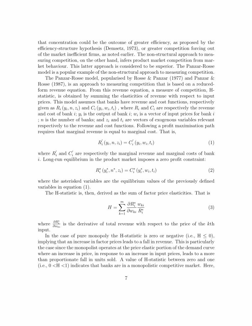
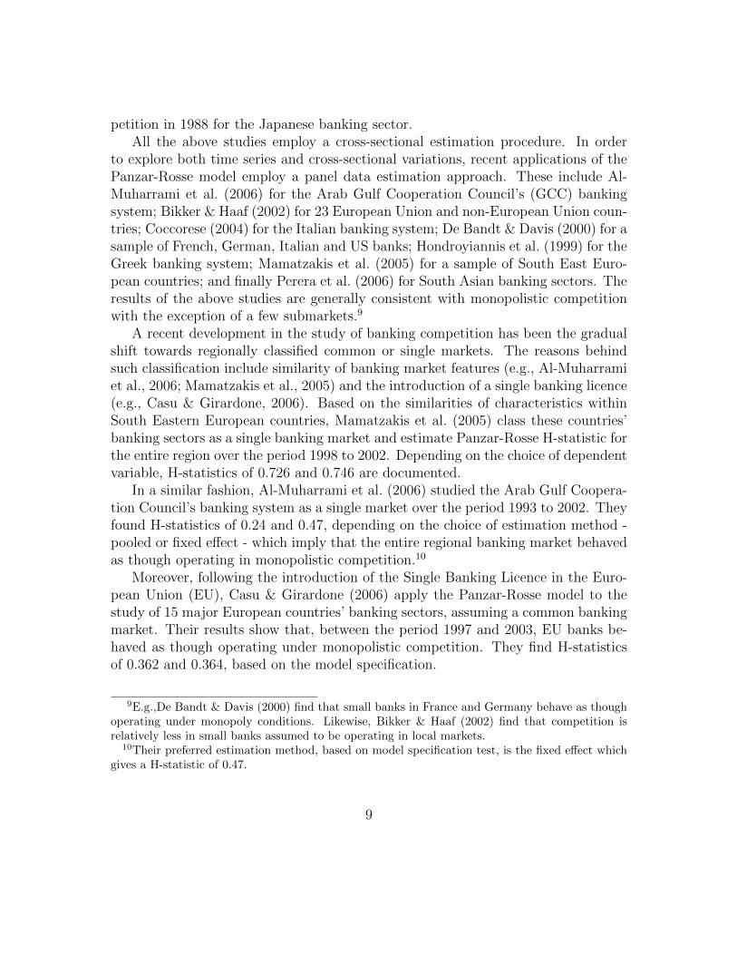
Despite record levels of new entry and foreign penetration, very high levels ofconcentration characterise African banking sectors. Over the period under consider-ation, the average Herfindahl-Hirschman Index (HHI) is as high as 2059, whilst thefive-bank concentration ratio stands at 77.29% for the whole African region.6 Onthe positive side, concentration assumed a downward trend across all the subregionsover the past few years, as can be seen in Figure 1. The Herfindahl-Hirschman In-dex (HHI) shows dramatic and consistent downward trend in all subregional bankingsectors except West Africa, where the trend is moderate. A similar trend is indicatedby five-bank concentration ratios,7 as shown in Figure 2.

As indicated earlier, banking sector concentration may not necessarily suggestless competition. As argued by Boone et al. (2005), fierce competition may drive outof the market the less efficient banks, with a resultant increase in banking marketconcentration. Hence, a non-structural measure of competition such as the Panzar-Rosse model which is based on reduced form revenue equation may be a superiormeasure of competition.

3. Panzar and Rosse model and related literature

Measurement of competition can take two approaches: the structural and thenon-structural. The structural approach to measuring competition, which under-pins the structural-conduct-performance paradigm, associates market power withthe degree of market concentration. The structural approach, thus, assumes lowercompetition in concentrated markets; more competition is associated with less con-centrated markets. The Herfindahl-Hirschman Index (HHI) plays a major role here.Concentration-based measures of competition have been criticised on the grounds

6HHI is measured as the sum of the squared market share of each bank in a given country foreach year. Market shares are measured in percentages. Hence, the HHI has an upper limit of10,000 where one firm commands 100% market share (i.e., monopoly) and a lower bound of zerofor perfect competition. HHI less than 1000 implies a highly competitive market. For a moderatelyconcentrated market HHI ranges between 1000 and 1800, whilst a concentrated market has HHIabove 1800.

7The only exception is West Africa where the trend is fairly upwards.

6

that concentration could be the outcome of greater efficiency, as proposed by theefficiency-structure hypothesis (Demsetz, 1973), or greater competition forcing outof the market inefficient firms, as noted earlier. The non-structural approach to mea-suring competition, on the other hand, infers product market competition from mar-ket behaviour. This latter approach is considered to be superior. The Panzar-Rossemodel is a popular example of the non-structural approach to measuring competition.

The Panzar-Rosse model, popularised by Rosse & Panzar (1977) and Panzar &Rosse (1987), is an approach to measuring competition that is based on a reduced-form revenue equation. From this revenue equation, a measure of competition, H-statistic, is obtained by summing the elasticities of revenue with respect to inputprices. This model assumes that banks have revenue and cost functions, respectivelygiven as Ri (yi, n, zi) and Ci (yi, wi, ti) , where Ri and Ci are respectively the revenueand cost of bank i; yi is the output of bank i; wi is a vector of input prices for bank i; n is the number of banks; and zi and ti are vectors of exogenous variables relevantrespectively to the revenue and cost functions. Following a profit maximisation pathrequires that marginal revenue is equal to marginal cost. That is,

R′

i (yi, n, zi) = C′

i (yi, wi, ti) (1)

where R′i and C

′i are respectively the marginal revenue and marginal costs of bank

i. Long-run equilibrium in the product market imposes a zero profit constraint:

R∗i (y∗i , n

∗, zi) = C∗i (y∗i , wi, ti) (2)

where the asterisked variables are the equilibrium values of the previously definedvariables in equation (1).

The H-statistic is, then, derived as the sum of factor price elasticities. That is

H =m∑k=1

∂R∗i

∂wki

wki

R∗i

(3)

where∂R∗i∂wki

is the derivative of total revenue with respect to the price of the kthinput.

In the case of pure monopoly the H-statistic is zero or negative (i.e., H ≤ 0),implying that an increase in factor prices leads to a fall in revenue. This is particularlythe case since the monopolist operates at the price elastic portion of the demand curvewhere an increase in price, in response to an increase in input prices, leads to a morethan proportionate fall in units sold. A value of H-statistic between zero and one(i.e., 0 <H <1) indicates that banks are in a monopolistic competitive market. Here,

7

an increase in factor prices increases average and marginal costs. This leads to theexit of loss-making banks and subsequent increase in revenue. In the extreme caseof perfect competition, with free entry and exit, an increase in factor prices causesrevenue to increase proportionally. Thus, H = 1 implies perfect competition.

The Panzar-Rosse model is theoretically consistent with the Lerner index, L, asit is shown to generalise to the following:

L =H

H − 1; (4)

Thus, the magnitude of H could be an indication of the level of the monopoly power(hence, competition) in the product market (see Vesala, 1995).

It must be emphasised that the Panzar-Rosse model relies on the assumptionthat banks are observed under long-run equilibrium.8 Long-run equilibrium requiresthat (risk-adjusted) returns are not statistically significantly correlated with inputprices (Shaffer, 1982). The application of the model to the banking sector furtherassumes that banks can be treated as single-product firms offering intermediationservices (De Bandt & Davis, 2000).

Starting from Shaffer (1982), the Panzar-Rosse model has been extensively ap-plied to the study of banking competition. Using a sample of US banking data forthe period 1979, Shaffer (1982) identifies a monopolistic competitive banking be-haviour. Other earlier applications of the model are in respect of Canadian banks(Nathan & Neave, 1989), European banks (Molyneux et al., 1994; Vesala, 1995) andJapanese banks (Molyneux et al., 1996). Nathan & Neave (1989) find monopolisticcompetition in the Canadian banking sector for the period 1983 and 1984 but perfectcompetition in the period 1982.

For a sample of European countries over the period 1986 to 1989, Molyneux et al.(1994) find that banks in France, Germany, Spain and the United Kingdom (UK)behave as though operating under monopolistic competitive conditions whilst thosein Italy are classed as though operating under monopoly or conjectural variationshort-run oligopoly conditions. Also, Vesala (1995) examines the Finnish bankingsystem over the period 1985 to 1992. He finds monopolistic competitive conditionsfor all years except 1989 and 1990 where the banking conditions are consistent withperfect competition. Finally, Molyneux et al. (1996) find conditions consistent withmonopoly or conjectural variation short-run oligopoly in 1986 and monopolistic com-

8This assumption is crucial for perfect competition and monopolistic competition conclusions tobe accurate (Panzar & Rosse, 1987).

8

petition in 1988 for the Japanese banking sector.All the above studies employ a cross-sectional estimation procedure. In order

to explore both time series and cross-sectional variations, recent applications of thePanzar-Rosse model employ a panel data estimation approach. These include Al-Muharrami et al. (2006) for the Arab Gulf Cooperation Council’s (GCC) bankingsystem; Bikker & Haaf (2002) for 23 European Union and non-European Union coun-tries; Coccorese (2004) for the Italian banking system; De Bandt & Davis (2000) for asample of French, German, Italian and US banks; Hondroyiannis et al. (1999) for theGreek banking system; Mamatzakis et al. (2005) for a sample of South East Euro-pean countries; and finally Perera et al. (2006) for South Asian banking sectors. Theresults of the above studies are generally consistent with monopolistic competitionwith the exception of a few submarkets.9

A recent development in the study of banking competition has been the gradualshift towards regionally classified common or single markets. The reasons behindsuch classification include similarity of banking market features (e.g., Al-Muharramiet al., 2006; Mamatzakis et al., 2005) and the introduction of a single banking licence(e.g., Casu & Girardone, 2006). Based on the similarities of characteristics withinSouth Eastern European countries, Mamatzakis et al. (2005) class these countries’banking sectors as a single banking market and estimate Panzar-Rosse H-statistic forthe entire region over the period 1998 to 2002. Depending on the choice of dependentvariable, H-statistics of 0.726 and 0.746 are documented.

In a similar fashion, Al-Muharrami et al. (2006) studied the Arab Gulf Coopera-tion Council’s banking system as a single market over the period 1993 to 2002. Theyfound H-statistics of 0.24 and 0.47, depending on the choice of estimation method -pooled or fixed effect - which imply that the entire regional banking market behavedas though operating in monopolistic competition.10

Moreover, following the introduction of the Single Banking Licence in the Euro-pean Union (EU), Casu & Girardone (2006) apply the Panzar-Rosse model to thestudy of 15 major European countries’ banking sectors, assuming a common bankingmarket. Their results show that, between the period 1997 and 2003, EU banks be-haved as though operating under monopolistic competition. They find H-statisticsof 0.362 and 0.364, based on the model specification.

9E.g.,De Bandt & Davis (2000) find that small banks in France and Germany behave as thoughoperating under monopoly conditions. Likewise, Bikker & Haaf (2002) find that competition isrelatively less in small banks assumed to be operating in local markets.

10Their preferred estimation method, based on model specification test, is the fixed effect whichgives a H-statistic of 0.47.

9

A further development worth noting is the proposition by Goddard & Wilson(2009) in relation to modifying the static Panzar-Rosse model to allow for partialadjustment towards equilibrium. This disequilibrium approach, in their view, isjustified because markets are not always in equilibrium. Hence, failure to take thisdynamic adjustment into account may render the Panzar-Rosse model misspecified.Using both simulated and real data for the banking sectors in the Group Seven (G7)countries, they find that the static H-statistic is severely biased towards zero whenthe adjustment towards equilibrium is partial rather than instantaneous. Similarly,Bikker et al. (2009) suggest that the H-statistics could be biased when scaled ratherthan unscaled revenue equation is estimated. Scaling revenue by total assets makesthe Panzar-Rosse model a price rather than a revenue equation. They further suggestthat controlling for total assets in the revenue equation also biases the Panzar-Rossemodel since this amounts to holding bank output fixed. In this study, these concernsare taken into consideration as part of robustness checks.

The present paper takes the view that increased regional integration coupledwith advances in information technology and the banking sector reforms justify theassumption of single banking markets within African subregions. Besides, the paperembraces recent development by applying a dynamic approach to the Panzar-Rossemodel.

4. Estimation method and data

Following from equations (1) and (2) and consistent with Bikker & Haaf (2002),the Panzar-Rosse model is implemented by formulating the marginal cost and marginalrevenue functions, imposing an equilibrium condition, and solving for the equilibriumoutput as a function of input prices and exogenous control variables. Assuming aCobb-Douglas technology, the marginal cost and revenue functions can be writtenas:

MCit = α0 + α1lnOutit +m∑k=1

βklnInpk,i,t +

p∑k=1

γklnXck,i,t (5)

and

MRit = φ0 + φ1lnOutit +

q∑h=1

ϕhXrh,i,t, (6)

where MCit and MRit are respectively the marginal costs and marginal revenueof bank i at time t; lnOutit and lnInpk,i,t are respectively the natural logarithmsof output and factor input k of bank i at time t; and lnXck,i,t and lnXrh,i,t arerespectively the natural logarithms of exogenous control variables k and h.

10

Imposing a zero profit constraint in equilibrium yields

lnOutit =(α0 − φ0 +

∑mk=1 βklnInpk,i,t + γkXck,i,t − ϕhXrh,i,t)

α1 − φ1

. (7)

Equation (7) translates into the following reduced form revenue empirical model:

lnRevit = α +J∑

j=1

βjlnWj,i,t +K∑k=1

γklnXk,i,t +N∑

n=1

ξnlnZn,t + εi,t, (8)

where subscripts i and t refer to bank i at time t; Rev is either total revenue orinterest revenue or the ratios of these to total assets; Wj is a three-dimensionalvector of input prices, namely, the unit price of fund(PF), unit price of labour(PL)and the unit price of capital(PC); Xk is a vector of bank-specific explanatory factorswhich may shift the revenue and cost functions; Zn is a vector of macroeconomicvariables; and εit is a composite error term including bank-fixed effects:

εi,t = µi + νi,t (9)

where µi is bank-fixed effects and νi,t, by assumption, is an independently and iden-tically distributed component with zero mean and variance σ2

v .Following the extant literature, PF is measured as the ratio of total interest

expenses to total deposits; PL is measured as the ratio of personnel expenses to totalasset; and PC is proxied by the ratio of other operating expenses to fixed assets.Bank-specific explanatory factors popular in the literature include total assets (TA)to control for size;11 the ratio of equity capital to total assets (EQTA), a proxy ofbanks’ leverage; the ratio of loans to total assets (NLTA) to account for credit riskexposure; the ratio of loan loss provisions to total loans (LLPL), which controls fordefault risk; and the ratio of other operating income to total assets (OITA).12

The H-statistic is then obtained as the sum of the coefficients of factor prices asfollows:

H =3∑

i=1

βi. (10)

11Following the literature (e.g., Mamatzakis et al., 2005) the natural log of total assets are ex-cluded from the models with scaled dependent variable.

12Other operating income is used as additional control variable only when interest income is usedas the dependent variable.

11

Consistent with the extant literature (e.g., Gunalp & Celik, 2006; Molyneux et al.,1996), a long-run equilibrium test is performed by replacing the dependent variablein equation (8) with the natural logarithm of return on assets (lnROA) as shownbelow:

lnROAit = α +J∑

j=1

βjlnWj,i,t +K∑k=1

γklnXk,i,t +N∑

n=1

ξnlnZn,t + εi,t. (11)

The sum of the elasticity of returns with respect to input prices, henceforth calledE-statistic, is obtained in a similar fashion as in equation (10).

Equations (8) and (11) are estimated using the panel fixed effect approach tocontrol for heterogeneity across banks whilst controlling for country level factorssuch as GDP growth and inflation.

In view of the criticism raised against the static Panzar & Rosse (1987) H-statistic,equation (11) is modified to take the suggested dynamics into account. Specifically,lagged dependent variable is included in the model as follows:

lnRevit = αlnRevi,t−1 +J∑

j=1

βjlnWj,i,t, +K∑k=1

γklnXk,i,t +N∑

n=1

ξnlnZn,t

+ εit. (12)

In this regard, it is possible to wipe out the unobserved firm specific effect by firstdifferencing equation (12) as follows:

∆lnRevit = α∆lnRevi,t−1 +J∑

j=1

βj∆lnWj,i,t +K∑k=1

γkln∆Xk,i,t +N∑

n=1

ξn∆lnZn,t

+ ∆εi,t, (13)

in which case a dynamic H-statistic can then be obtained as:

H =

∑3i=1 βi

1 − α. (14)

12

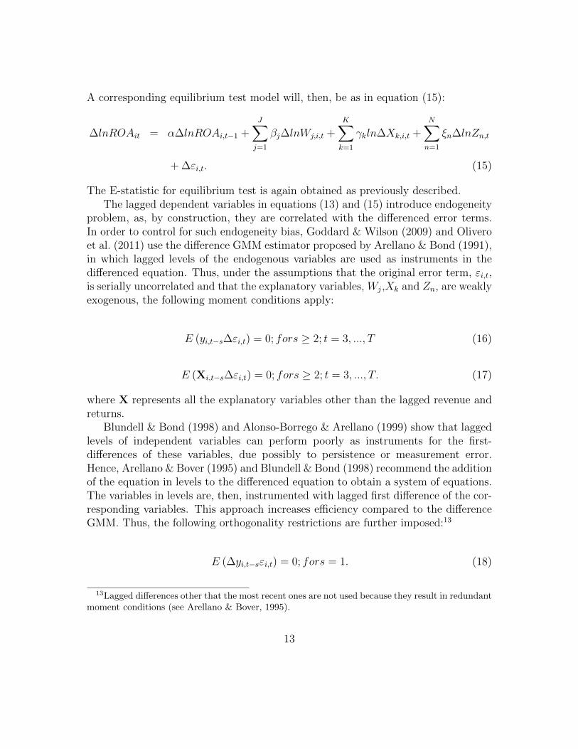
A corresponding equilibrium test model will, then, be as in equation (15):

∆lnROAit = α∆lnROAi,t−1 +J∑

j=1

βj∆lnWj,i,t +K∑k=1

γkln∆Xk,i,t +N∑

n=1

ξn∆lnZn,t

+ ∆εi,t. (15)

The E-statistic for equilibrium test is again obtained as previously described.The lagged dependent variables in equations (13) and (15) introduce endogeneity

problem, as, by construction, they are correlated with the differenced error terms.In order to control for such endogeneity bias, Goddard & Wilson (2009) and Oliveroet al. (2011) use the difference GMM estimator proposed by Arellano & Bond (1991),in which lagged levels of the endogenous variables are used as instruments in thedifferenced equation. Thus, under the assumptions that the original error term, εi,t,is serially uncorrelated and that the explanatory variables, Wj,Xk and Zn, are weaklyexogenous, the following moment conditions apply:

E (yi,t−s∆εi,t) = 0; fors ≥ 2; t = 3, ..., T (16)

E (Xi,t−s∆εi,t) = 0; fors ≥ 2; t = 3, ..., T. (17)

where X represents all the explanatory variables other than the lagged revenue andreturns.

Blundell & Bond (1998) and Alonso-Borrego & Arellano (1999) show that laggedlevels of independent variables can perform poorly as instruments for the first-differences of these variables, due possibly to persistence or measurement error.Hence, Arellano & Bover (1995) and Blundell & Bond (1998) recommend the additionof the equation in levels to the differenced equation to obtain a system of equations.The variables in levels are, then, instrumented with lagged first difference of the cor-responding variables. This approach increases efficiency compared to the differenceGMM. Thus, the following orthogonality restrictions are further imposed:13

E (∆yi,t−sεi,t) = 0; fors = 1. (18)

13Lagged differences other that the most recent ones are not used because they result in redundantmoment conditions (see Arellano & Bover, 1995).

13

E (∆Xi,t−sεi,t) = 0; fors = 1. (19)

By construct, first order serial correlation is expected in the first differencedequation. Hence, in order to rule out first order serial correlation in levels, a test ofsecond order serial correlation in the differenced equation is performed (Roodman,2009).Next, a Hansen test of over-identifying restrictions is employed to test thevalidity of the over-identification restrictions. As a final step, standard errors arecorrected for small sample bias based on the two-step covariance matrix attributedto Windmeijer (2005).

In view of the above, the study first estimates the static Panzar-Rosse model andthe corresponding equilibrium test model (equations (8) and (11), respectively) usingthe panel fixed effect estimation method. This approach helps to control for unob-served heterogeneity. Second, the dynamic models (equations (12), (13) and (15))are estimated using the dynamic system GMM estimator as robustness checks. Timedummies are included in all models to control for time-specific effects including thepossibility of linear association between input prices and time (Perera et al., 2006).For all estimations, a Wald test is performed to ascertain whether the H-statistics aresignificantly different from zero and one. Next, a similar test is conducted to verifyif the E-statistics are significantly not different from zero - a necessary condition forlong-run equilibrium.

Bank-level data over the period 2003 to 2009 is obtained from the BankScopedatabase. A few data exclusion criteria are applied. First, all bank observations withnegative values of equity are dropped from the data. Second, a few bank observationswith interest expenses exceeding 100% of total deposits are dropped.14 The finalsample contains 845 observations of Southern African banks, 832 observations ofWest African banks, 484 observations of North African banks and 603 observationsof East African banks. Full country-year observations and subregional totals aregiven in Table 1. Macroeconomic variables are sourced from World Bank (2011)World Development Indicators. Sample descriptive statistics and correlation matrixare shown in Tables 2 and 3, respectively.

5. Results

This section presents the estimations results of the static and dynamic Panzar-Rosse models for all the subregions. From these estimation results, the static and

14The subsequent results, however, do not significantly change when these exclusion criteria arerelaxed.

14

dynamic H-statistics and their corresponding E-statistics are computed. Alternativedependent variables (total revenue and interest revenue) are employed as robustnesschecks and a series of diagnostic tests carried out.

5.1. Static H-statistic

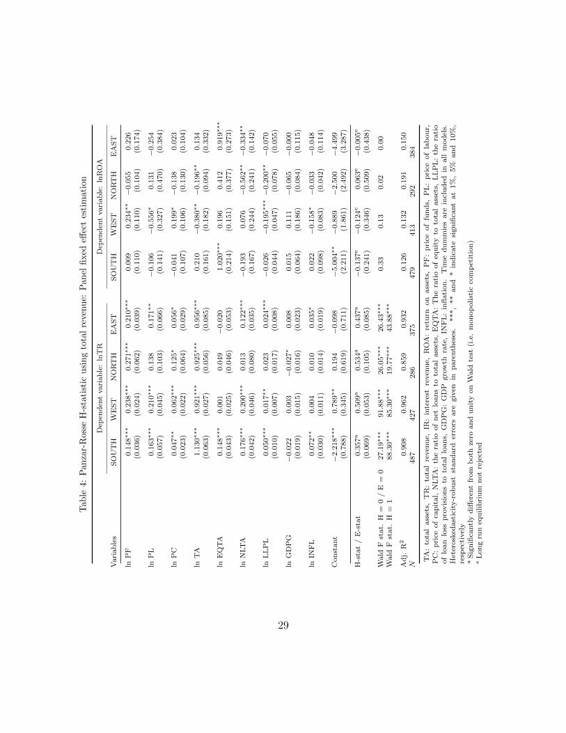
First, the static Panzar-Rosse model is estimated using the panel fixed effect es-timation technique. Columns 1-4 of Table 4 show that the H-statistics are positiveand statistically significant for all the subregional banking markets. North Africahas the highest H-statistic (0.534), followed by West Africa (0.509), East Africa(0.437) and Southern Africa (0.357). The Wald test confirms that the H-statisticsare significantly different from both zero and unity for all subregions. The findingssuggest that the subregional banking markets are characterised by monopolistic com-petitive behaviour. Thus, competition coexists with high levels of banking marketconcentration, suggesting contestable market behaviour.

Following Vesala (1995), the H-statistic can be employed as a continuous measureof competition. In this regard, banking sector competition in Africa in recent timesis somehow comparable to that existing in other single banking markets in emergingeconomies. However, a fair amount of caution is recommended due to cross-marketdifferences not captured by the model. With the exception of Southern Africa, the H-statistic is higher for all subregions compared to those documented in Al-Muharramiet al. (2006) for the GCC banking system (see Section 3). However, for all subregions,the H-statistic is significantly lower than that documented in Mamatzakis et al.(2005) for South Eastern European countries. The findings reported here are notdirectly comparable to Casu & Girardone (2006) due to significant differences inmodel specification.15

Given that most of the studies on banking competition (cited above) report resultsthat are consistent with monopolistic competition, the findings of this study suggestthat recent financial sector reforms in Africa may have had some beneficial effects interms of market discipline.

In line with previous studies (e.g., Bikker & Haaf, 2002; Coccorese, 2004; Molyneuxet al., 1994; Yeyati & Micco, 2007), the coefficient of unit price of funds is positiveand statistically significant as expected for all subregions. Likewise, the unit price oflabour is positive and statistically significant for all subregions except North Africa.Also, the unit price of capital (other operating expenses) is positive and statistically

15Although the H-statistics reported here are larger than those reported in Casu & Girardone(2006) for 15 major European countries’ banking market, their control variables somehow differfrom those used in this paper.

15

significant for all subregions. Price of funds seems to be the biggest contributor to theH-statistic for all subregions except Southern Africa, where the biggest contributoris the price of labour. This highlights the strong effect of interest rate liberalisation.

In relation to the control variables, it is observed that bank size (proxied bytotal assets) is positive and statistically significant for all subregions, suggesting theexistence of economies of scale. The ratio of equity to total assets is mostly positive(the exception is East Africa) but significant only for Southern Africa. Consistentwith Mamatzakis et al. (2005) and Bikker & Haaf (2002), the ratio of loans to totalassets is always positive as expected and significant for all subregions except forNorth Africa. Also, in line with Mamatzakis et al. (2005) and Al-Muharrami et al.(2006), the ratio of loan loss provisions to total assets is positive for all subregionsand statistically significant except for North Africa. This is consistent with the viewthat higher default risk is matched with higher reward (e.g., Al-Muharrami et al.,2006).

As regards the macroeconomic environment, the impact of GDP growth is mixed:it is negative for the Southern and North African subregions but positive for Westand East Africa. However, it is statistically significant only for the North Africansubregion. The coefficient of inflation is positive as in Mamatzakis et al. (2005), andsignificant only for the Southern and East African subregions.

As the validity of the H-statistics depends on the assumption of long-run equi-librium, Table 4 also provides the results of the equilibrium test in columns 4-8,obtained from equation (11) where ROA is the dependent variable. The Wald testsresults show that the E-statistics are not statistically different from zero, suggestingthat the banks are observed under long long-run equilibrium.

The results presented above are subjected to a series of robustness checks. First,given that a significant number of studies do scale revenue by total assets (e.g.,Al-Muharrami et al., 2006; Claessens & Laeven, 2004; Hondroyiannis et al., 1999;Mamatzakis et al., 2005; Perera et al., 2006), whilst several others do not (e.g.,Bikker & Haaf, 2002; Coccorese, 2004; Gunalp & Celik, 2006), and the concernsraised in Bikker et al. (2009) about possible bias arising from misspecification ofthe model, the paper compares the results above with the models using the ratioof revenue to total assets as the dependent variables. The results are presented inTable 5

As noted in Table 5, the main findings are qualitatively similar to those presentedearlier, notwithstanding some apparent slight differences in the magnitude of the H-statistics; The H-statistics are all statistically significantly different from both zeroand unity. In addition, similar results are obtained when total assets are dropped

16

from the above estimations.16 The existence of long-run equilibrium is also notrejected, as indicated in columns 4-8 of the table.

As interest-generating activities have been the tradition in African banking sec-tors for many years, results for interest income as a dependent variable are alsoprovided in Table 6. The results show that the H-statistic is highest (0.638) for theWest African subregional banking market, followed by North African (0.514), South-ern African (0.490) and East African (0.444). Thus, the East African banking marketis the least competitive in terms of interest income, while Southern Africa is the leastcompetitive in terms of total banking activity. In comparison with Al-Muharramiet al. (2006) the estimates of the level of banking market competition are found to behigher for all African subregions, but lower when compared with Mamatzakis et al.(2005). Columns 4-8 of the table confirm that the banks are observed under long-runequilibrium.

As for input prices, unit prices of funds and labour are positive and significant forall subregions. However, the unit price of capital, though positive for all subregions,is significant only in the case of West Africa. Also, the coefficient of the unit price offunds is significantly higher in magnitude compared to the results for the total rev-enue equation and remains the biggest contributor to the H-statistic. This, coupledwith the fact that the H-statistic is higher for all subregions except North Africa,suggests a higher degree of competition in interest-generating activities relative tototal banking activities.

As far as the control variables are concerned, Table 6 shows that the ratio of equityto total assets, though always positive, is statistically insignificant for all subregions.Also, the coefficients of the ratio of loans to total assets are relatively higher inmagnitude compared to the previous results. The ratio of other income to totalassets has the expected negative sign for all subregions but is statistically significantonly for Southern and West African banking markets. Thus, the engagement in otherincome-generating activities constrains banks’ ability to generate interest income(Bikker & Haaf, 2002). The sign of the coefficient of GDP growth is again mixedbut insignificant for all subregions, whilst inflation is positive and significant only forSouthern Africa.

The E-statistics reported in columns 4-8 of Table 6 do not reject long-run equi-

16These estimations control for capacity indicators such as total fixed assets or equity (e.g.,De Bandt & Davis, 2000; Gischer & Stiele, 2009; Murjan & Ruza, 2002; Vesala, 1995; Yildirim &Philippatos, 2007). Controlling for fixed assets rather than total assets does not hold banks’ outputconstant, and it is therefore appropriate. The results are not presented here, for brevity, and areavailable upon request.

17

librium. As shown by the Wald test, the E-statistics are all not statistically differentfrom zero.

The results presented so far suggest that banking competition in Africa is gen-erally comparable to regional markets in other emerging economies. As in the totalrevenue model, the findings are robust to using the ratio of interest revenue to totalassets as the dependent variable. Furthermore, the findings are robust to droppingtotal assets from the model.

5.2. Dynamic H-statistic

In this section, the dynamic version of the results presented above is discussed.The estimation results for the models using total revenue as the dependent variableare shown in Table 7. The maximum lag dependent variable is restricted to one inall models in order to restrain the number of moment conditions. The lag dependentvariable is positive and significant; the Hansen test p-values are all well above 0.1,justifying the validity of the over-identification restriction; and, finally, the absenceof second-order serial correlation is not rejected. Thus, the diagnostic tests justifythe use of a dynamic model.

Table 7 shows that the H-statistic is positive and significantly different fromboth zero and one for all subregions, suggesting a monopolistic competitive marketstructure in all the banking markets. It is worth noting that the H-statistics are muchlarger in magnitude compared to the results in Table 4. This finding lends supportto the view of Goddard & Wilson (2009) that the static H-statistic is downwardbiased if the adjustment towards equilibrium is partial rather than instantaneous.The results further show that, when dynamics are taken into account, H-statistic ishighest (0.605) in East Africa; and it is least (0.517) in Southern Africa. The resultfor East Africa is not surprising given the extent of recent reforms and cross-borderbanking. Even after taking partial adjustment to equilibrium into account, the H-statistics for all subregions are slightly lower than those reported in Mamatzakiset al. (2005), except when interest revenue is considered.

Consistent with the previous results (Table 4), the price of funds is positive andsignificant for all subregions. Similarly, the price of labour is positive and significantfor all subregions, whilst the price of capital is significantly positive for only theNorth and East African subregional banking markets. As in previous results, theprice of funds seems to be the biggest contributor to the H-statistic.

As far as the control variables are concerned, the noticeable changes are that theratio of net loans to total assets is now significant only for East Africa. GDP growthis positive and significant only for East Africa and inflation is significantly positiveonly for Southern Africa. The ratio of loan loss provisions to total assets is now not

18

significant for West AfricaThe results of the equilibrium test (equation (15)) are also presented in columns

4-8 (Table 7). The diagnostic tests are satisfactory, and long-run equilibrium is notrejected.17

As in the estimation of the static models, the robustness of these results is as-sessed. First, similar results are obtained when total revenue is replaced with theratio of total revenue to total assets as the dependent variable, as shown in Table 8.Compared to the preceding results, the H-statistics are slightly larger. Also, the H-statistic for West Africa is significantly different from one only at the margin. Thesenotwithstanding, the main findings remain unchanged.

Finally, results of the dynamic models in which interest revenue is the dependentvariable are also provided in Table 9. The results are not qualitatively different fromthe above except that the West and East African subregional banking markets nowhave higher H-statistics compared with the findings of Mamatzakis et al. (2005). Allthe diagnostic tests are, again, satisfactory. The H-statistics are, as before, higher inmagnitude compared to those shown in Table 6. Consistent with the results in Table6, the H-statistic is highest in West Africa (0.810). However, East Africa also has ahigh H-statistic of 0.780. Similar results are obtained when the dependent variableis the ratio of interest revenue to total assets.

6. Conclusion

This study examines banking competition across subregional banking markets inAfrica. Assuming common markets within each subregion due to increased regionalintegration and cross-border banking, the non-structural approach to measuring com-petition, proposed by Rosse & Panzar (1977) and Panzar & Rosse (1987), is used toestimate the degree of competition in each of the subregional banking market. Theresults suggest the existence of monopolistic competition across African subregionalbanking markets. These results are consistent with several recent studies for otherparts of the world, particularly in emerging economies, suggesting that recent struc-tural reforms within Africa may have had significant effects as far as banking sectorcompetition is concerned.

The results are robust to alternative views of banking activities (i.e., interest-generating activities versus total banking activities) as well as alternative specifi-cations and estimators. In particular, whilst the existence of long-run equilibrium,

17The lagged dependent variable for the equilibrium test model is, however, not significant forNorth Africa. Thus, a fair amount of caution is to be exercised in interpreting the results.

19

as a necessary condition, is verified for all model specifications, the robustness ofthe results in relation to the possibility of partial adjustment towards equilibrium isfurther assessed. In the empirical implementation, therefore, a dynamic approach isalso used to estimate the Panzar-Rosse model to obtain a dynamic H-statistic forcomparison with the static H-statistic. Whilst the results confirm the downwardsbias of the static H-statistic, monopolistic competition cannot be ruled out.

The findings of this paper have policy significance because of the possible linkbetween banking competition and efficient financial intermediation, bank profitabilityand stability. The results also offer a yardstick against which to measure the successof several years of regional integration and cross-border banking in Africa.

Acknowledgement

I would like to thank Barbara Roberts for her support and helpful comment. I amalso thankful to the editor, Jonathan A. Batten, Emerging Markets Review, and ananonymous referee for their constructive comments. All errors, logically, are mine.

References

Al-Muharrami, S., Matthews, K., & Khabari, Y. (2006). Market structure andcompetitive conditions in the Arab GCC banking system. Journal of Banking &Finance, 30 , 3487–3501.

Allen, F., Otchere, I., & Senbet, L. W. (2011). African financial systems: A review.Review of Development Finance, 1 , 79 – 113.

Alonso-Borrego, C., & Arellano, M. (1999). Symmetrically normalized instrumental-variable estimation using panel data. Journal of Business & Economic Statistics ,17 , 36–49.

Arellano, M., & Bond, S. (1991). Some tests of specification for panel data: MonteCarlo evidence and an application to employment equations. Review of EconomicStudies , 58 , 277–97.

Arellano, M., & Bover, O. (1995). Another look at the instrumental variable estima-tion of error-components models. Journal of Econometrics , 68 , 29–51.

Biekpe, N. (2011). The competitiveness of commercial banks in Ghana. AfricanDevelopment Review , 23 , 75–87.

20

Bikker, J., & Haaf, K. (2002). Competition, concentration and their relationship:An empirical analysis of the banking industry. Journal of Banking and Finance,26 , 1291–2214.

Bikker, J. A., Shaffer, S., & Spierdijk, L. (2009). Assessing competition with thePanzar-Rosse Model: The role of scale, costs, and equilibrium. Working Papers09-27 Utrecht School of Economics.

Blundell, R., & Bond, S. (1998). Initial conditions and moment restrictions in dy-namic panel data models. Journal of Econometrics , 87 , 115–143.

Boone, J., Griffith, R., & Harrison, R. (2005). Measuring competition. WorkingPaper No. 022, Advanced Institute of Management Research.

Casu, B., & Girardone, C. (2006). Bank competition, concentration and efficiencyin the single European market. The Manchester School , 74 , 441–468.

Claessens, S., & Laeven, L. (2004). What drives bank competition? Some interna-tional evidence. Journal of Money, Credit and Banking , 36 , pp. 563–583.

Coccorese, P. (2004). Banking competition and macroeconomic conditions: A dis-aggregate analysis. Journal of International Financial Markets, Institutions andMoney , 14 , 203–219.

De Bandt, O., & Davis, E. P. (2000). Competition, contestability and market struc-ture in European banking sectors on the eve of EMU. Journal of Banking &Finance, 24 , 1045–1066.

Demsetz, H. (1973). Industry structure, market rivalry, and public policy. Journalof Law and Economics , 16 , 1–9.

Gischer, H., & Stiele, M. (2009). Competition tests with a non-structural model:The Panzar-Rosse method applied to Germany’s savings banks. German EconomicReview , 10 , 50–70.

Goddard, J., & Wilson, J. O. (2009). Competition in banking: A disequilibriumapproach. Journal of Banking & Finance, 33 , 2282–2292.

Gunalp, B., & Celik, T. (2006). Competition in the Turkish banking industry.Applied Economics , 38 , 1335–1342.

21

Hondroyiannis, G., Lolos, S., & Papapetrou, E. (1999). Assessing competitive con-ditions in the Greek banking system. Journal of International Financial Markets,Institutions and Money , 9 , 377–391.

Mamatzakis, E., Staikouras, C., & Koutsomanoli-Fillipaki, N. (2005). Competitionand concentration in the banking sector of the South Eastern European region.Emerging Markets Review , 6 , 192–209.

Molyneux, P., Lloyd-Williams, D. M., & Thornton, J. (1994). Competitive conditionsin European banking. Journal of Banking & Finance, 18 , 445–459.

Molyneux, P., Thornton, J., & Michael Llyod-Williams, D. (1996). Competition andmarket contestability in Japanese commercial banking. Journal of Economics andBusiness , 48 , 33–45.

Murjan, W., & Ruza, C. (2002). The competitive nature of the Arab Middle Easternbanking markets. International Advances in Economic Research, 8 , 267–274.

Nathan, A., & Neave, E. H. (1989). Competition and contestability in Canada’sfinancial system: Empirical results. The Canadian Journal of Economics / Revuecanadienne d’Economique, 22 , pp. 576–594.

Olivero, M. P., Li, Y., & Jeon, B. N. (2011). Competition in banking and the lendingchannel: Evidence from bank-level data in Asia and Latin America. Journal ofBanking & Finance, 35 , 560–571.

Panzar, J. C., & Rosse, J. N. (1987). Testing for “monopoly” equilibrium. TheJournal of Industrial Economics , 35 , 443–456.

Perera, S., Skully, M., & Wickramanayake, J. (2006). Competition and structureof South Asian banking: A revenue behaviour approach. Applied Financial Eco-nomics , 16 , 789–801.

Roodman, D. (2009). How to do xtabond2: An introduction to difference and systemGMM in Stata. Stata Journal , 9 , 86–136.

Rosse, J. N., & Panzar, J. C. (1977). Chamberlin vs. Robinson: An empirical studyof monopoly rents. Bell Laboratories Economic Discussion Paper 90.

Schaeck, K., Cihak, M., & Wolfe, S. (2009). Are competitive banking systems morestable? Journal of Money, Credit and Banking , 41 , 711–734.

22

Senbet, L. W., & Otchere, I. (2006). Financial sector reforms in Africa: Perspectiveson issues and policies. In F. Bourguignon, & B. Pleskovic (Eds.), Annual WorldBank conference on development economics: Growth and integration (pp. 81 –119). Washington, D.C.: The World Bank.

Shaffer, S. (1982). A nonstructural test of competition in financial markets. InBank structure and competition. Conference proceedings, Federal Reserve Bank ofChicago (pp. 225–243).

Simpasa, A. M. (2011). Competitive conditions in Tanzanian commercial bankingindustry. African Development Review , 23 , 88–98.

Vesala, J. (1995). Testing for competition in banking: Behavioral evidence fromFinland. Bank of Finland Studies, E:1, Helsinki.

Windmeijer, F. (2005). A finite sample correction for the variance of linear efficienttwo-step GMM estimators. Journal of Econometrics , 126 , 25–51.

World Bank (2011). World development indicators (edition: April 2011). ESDSInternational, University of Manchester , .

Yeyati, E. L., & Micco, A. (2007). Concentration and foreign penetration in LatinAmerican banking sectors: Impact on competition and risk. Journal of Banking& Finance, 31 , 1633–1647.

Yildirim, H. S., & Philippatos, G. C. (2007). Restructuring, consolidation and com-petition in Latin American banking markets. Journal of Banking & Finance, 31 ,629–639.

23

Figure 1: Evolution of banking sector concentration (HHI) by subregion.

1000

2000

3000

4000

5000

Her

finda

hl-H

irsch

man

Inde

x (H

HI)

2002 2004 2006 2008 2010Year

South WestNorth East

24

Figure 2: Evolution of banking sector concentration (CR5) by subregion.

6070

8090

100

Five

-ban

k co

ncen

tratio

n ra

tio(C

R5)

2002 2004 2006 2008 2010Year

South WestNorth East

25

Table 1: Sample number of banks by country, year and subregion

Year

Country 2002 2003 2004 2005 2006 2007 2008 2009 Total

Panel 1: Southern AfricaAngola 5 9 10 11 13 12 13 12 85Botswana 1 4 6 7 9 9 11 10 57Congo, D.R. OF 1 3 5 9 9 7 9 6 49Lesotho 2 3 3 2 3 3 3 2 21Madagascar 3 5 5 5 5 4 5 5 37Malawi 7 10 10 9 9 8 11 11 75Mauritius 2 11 13 13 14 15 16 12 96Mozambique 2 4 4 6 6 9 11 11 53Namibia 1 1 2 7 8 7 8 7 41Seychelles 0 1 2 4 4 4 3 2 20South Africa 2 3 11 25 30 34 41 37 183Swaziland 2 5 6 6 5 5 5 5 39Zambia 5 12 12 12 12 14 12 10 89

Regional total 33 71 89 116 127 131 148 130 845

Panel 2: West AfricaBenin 4 6 4 6 6 6 6 5 43Burkina Faso 3 5 7 7 8 7 6 5 48Cameroon 5 9 10 11 12 9 6 5 67Cape Verde 2 2 2 3 2 2 2 1 16Gabon 1 1 1 2 2 2 2 2 13Gambia 2 3 3 4 5 4 4 3 28Ghana 4 4 5 9 9 21 23 22 97Ivory Coast 8 11 11 13 12 11 10 6 82Mali 5 5 6 6 7 7 7 6 49Mauritania 5 7 7 8 6 5 4 5 47Nigeria 22 28 36 26 22 23 19 17 193Senegal 9 10 10 8 8 8 7 7 67Sierra Leone 4 5 6 5 8 8 8 7 51Togo 1 3 4 4 5 5 5 4 31

Regional total 75 99 112 112 112 118 109 95 832

Panel 3: North AfricaAlgeria 8 9 14 12 15 15 15 12 100Morocco 3 5 7 7 10 17 17 15 81Niger 1 3 4 4 5 5 4 4 30Sudan 8 10 7 9 13 17 18 17 99Tunisia 10 19 20 21 25 27 29 23 174

Regional total 30 46 52 53 68 81 83 71 484

Panel 4: East AfricaBurundi 5 5 5 5 4 4 3 3 34Ethiopia 1 8 8 9 9 10 8 9 62Kenya 12 26 27 30 30 35 35 34 229Rwanda 1 3 4 4 5 4 3 3 27Tanzania 1 2 7 21 25 24 23 22 125Uganda 9 15 16 16 17 16 18 19 126

Regional Regional total 29 59 67 85 90 93 90 90 603

Source: Fitch-IBCA’s Bankscope database and own calculation

26

Tab

le2:

Des

crip

tive

Sta

tist

ics

Cou

ntr

yT

AT

RIR

RO

AP

FP

LP

CN

LT

AE

QT

AL

LP

LG

DP

GIN

FL

Pan

el1:

Sou

ther

nA

fric

aA

ngola

1329.5

4135.8

081.8

71.2

52.1

31.7

967.6

129.1

714.7

08.3

713.0

232.5

1B

ots

wan

a563.6

785.9

968.1

22.9

011.6

42.1

3256.0

446.6

313.2

31.4

62.9

69.3

8C

on

go

D.R

.112.4

216.8

59.1

31.4

01.5

62.6

1184.3

031.6

411.4

26.9

85.5

915.6

7L

esoth

o207.1

526.7

618.4

41.7

83.5

82.6

0125.3

619.5

57.7

31.5

63.1

49.4

4M

ad

agasc

ar

232.3

122.1

117.3

32.6

52.9

81.1

8166.8

947.0

510.5

12.0

53.4

510.5

2M

ala

wi

91.7

718.7

211.4

92.2

36.3

45.3

6107.4

335.4

216.7

41.3

75.8

611.0

6M

au

riti

us

1033.2

490.1

558.1

21.0

84.8

90.8

8417.6

951.2

813.6

00.7

13.9

66.5

1M

oza

mb

iqu

e361.9

651.4

633.1

40.1

43.8

74.7

4129.6

835.3

718.1

82.2

87.2

69.1

2N

am

ibia

996.5

0139.7

9110.8

71.9

58.2

12.3

0142.5

581.2

119.0

80.9

84.2

56.5

8S

eych

elle

s222.1

320.8

311.8

11.9

01.2

20.6

7250.5

328.8

16.2

20.5

83.6

210.4

5S

ou

thA

fric

a23689.3

72663.1

81961.8

82.5

411.7

82.8

7779.3

657.9

517.3

82.0

53.4

96.8

5S

wazi

lan

d158.4

622.5

615.3

62.8

88.3

63.3

4223.7

564.1

119.3

80.1

42.6

07.3

7Z

am

bia

202.5

131.3

219.5

21.1

85.2

84.8

7220.7

729.7

514.7

63.7

05.6

215.1

0

Aver

age

5554.4

5611.6

7445.0

21.8

56.5

92.8

9325.2

844.7

815.1

42.6

95.2

511.7

6

Pan

el2:

Wes

tA

fric

aB

enin

247.5

023.1

815.3

7−

0.2

72.5

51.8

6133.1

256.1

99.2

12.3

74.0

23.3

4B

urk

ina

Faso

221.7

823.3

015.6

50.6

82.6

01.9

694.3

460.2

98.1

72.6

35.1

73.1

8C

am

eroon

377.2

439.4

522.2

21.1

43.2

51.9

3104.3

950.7

711.4

71.8

23.2

32.4

1C

ap

eV

erd

e82.0

37.2

65.2

02.2

72.3

42.9

8139.3

344.7

316.0

41.7

36.8

22.3

6G

ab

on

93.6

311.1

38.6

01.2

86.9

24.4

491.6

256.4

541.4

4−

0.4

51.9

82.4

3G

am

bia

61.8

711.2

56.8

22.9

53.9

32.7

791.7

729.5

514.2

82.6

05.4

26.9

1G

han

a283.6

148.4

535.5

91.7

98.7

04.3

4134.5

542.1

215.3

73.1

16.2

815.3

8Iv

ory

Coast

378.2

543.7

324.6

6−

0.1

73.9

13.7

7184.0

859.5

810.2

30.8

40.9

53.0

2M

ali

271.7

023.2

715.2

11.2

31.5

51.9

169.1

257.2

510.7

71.9

54.7

92.7

8M

au

rita

nia

119.6

911.6

46.5

81.8

72.5

81.8

9117.3

950.8

723.8

74.1

24.7

27.2

2N

iger

ia1893.1

9243.7

6160.7

92.0

37.7

02.7

2160.0

232.4

917.0

81.4

26.9

312.4

4S

eneg

al

336.0

934.6

125.6

10.8

82.3

01.6

2138.2

957.7

98.9

81.3

84.1

02.0

2S

ierr

aL

eon

e37.8

57.3

74.3

32.6

23.6

03.9

3105.3

222.9

420.2

38.7

18.2

212.0

3T

ogo

1180.0

5148.4

991.7

82.0

02.2

32.6

794.3

252.5

914.1

9−

1.8

42.4

93.1

0

Aver

age

666.7

185.2

756.4

91.4

24.7

42.7

8130.9

146.0

614.5

42.1

85.0

27.2

7

Pan

el3:

Nort

hA

fric

aA

lger

ia4125.8

5215.0

4148.4

51.0

62.8

20.8

069.5

941.8

714.0

33.3

63.7

03.3

1M

oro

cco

7261.7

7466.9

0382.0

01.7

43.8

31.8

587.6

767.8

312.1

11.0

64.8

02.1

9N

iger

119.5

312.4

97.6

90.4

51.7

12.0

1118.1

856.7

09.6

20.4

94.1

63.1

0S

ud

an

953.3

778.0

745.1

01.8

45.0

92.2

584.8

631.4

017.1

54.1

07.3

49.6

7T

un

isia

1012.0

573.5

453.0

60.8

812.0

71.3

790.7

868.5

820.2

82.5

14.8

63.5

8

Aver

age

2634.0

0162.7

2123.2

61.2

36.7

11.5

486.4

154.7

316.3

22.5

25.0

74.5

0

Pan

el4:

East

Afr

ica

Bu

nru

nd

i52.7

57.2

84.8

42.0

24.8

02.6

266.4

754.6

313.7

24.1

43.0

58.9

3E

thio

pia

721.8

947.3

326.9

02.4

52.2

01.0

289.3

254.0

312.3

21.3

99.2

915.9

5K

enya

340.5

545.7

030.6

61.5

14.7

73.1

1127.4

953.4

718.9

92.3

74.2

612.7

1R

wan

da

90.1

110.4

27.5

41.2

74.7

42.6

0116.4

743.0

110.0

93.1

47.3

49.9

1T

an

zan

ia202.1

125.3

418.1

51.5

04.6

93.4

6318.8

145.8

513.1

11.8

86.9

98.0

7U

gan

da

167.0

626.2

421.0

32.5

35.0

36.0

8241.2

047.4

616.4

42.0

87.9

08.0

2

Aver

age

287.3

734.6

523.3

11.8

34.5

43.2

2182.6

650.2

615.8

62.2

36.1

710.7

6

Valu

esare

inm

illion

sof

US

$fo

rT

A,

TR

an

dIR

an

dp

erce

nta

ges

for

all

oth

ervari

ab

les.

TA

:to

tal

ass

ets,

TR

:to

tal

reven

ue,

IR:

inte

rest

reven

ue,

RO

A:

retu

rnon

ass

ets,

PF

:p

rice

of

fun

ds,

PL

:p

rice

of

lab

our,

PC

:p

rice

of

cap

ital,

NLT

A:

the

rati

oof

net

loan

sto

tota

lass

ets,

EQ

TA

:T

he

rati

oof

equ

ity

toto

tal

ass

ets,

LL

PL

:th

era

tio

of

loan

loss

pro

vis

ion

sto

tota

llo

an

s,G

DP

G:

GD

Pgro

wth

rate

,IN

FL

:in

flati

on

.

27

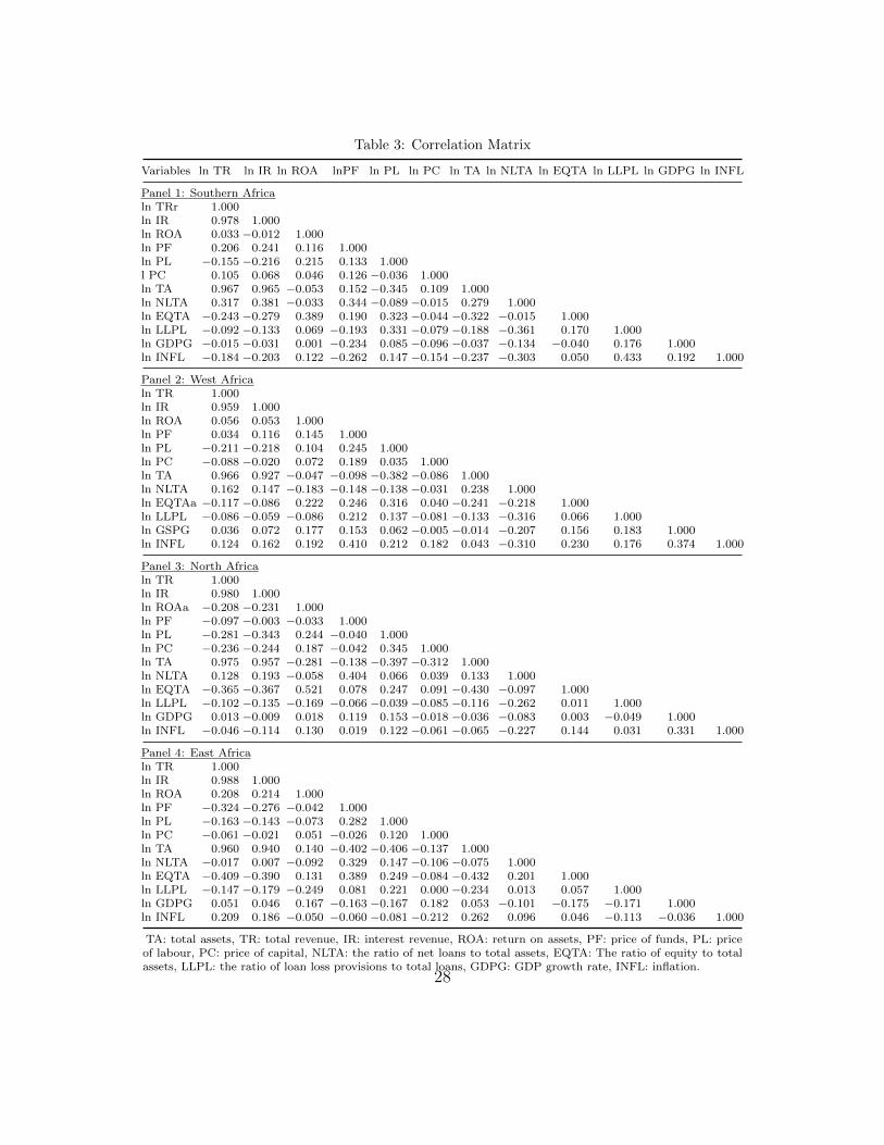
Table 3: Correlation Matrix

Variables ln TR ln IR ln ROA lnPF ln PL ln PC ln TA ln NLTA ln EQTA ln LLPL ln GDPG ln INFL

Panel 1: Southern Africaln TRr 1.000ln IR 0.978 1.000ln ROA 0.033 −0.012 1.000ln PF 0.206 0.241 0.116 1.000ln PL −0.155 −0.216 0.215 0.133 1.000l PC 0.105 0.068 0.046 0.126 −0.036 1.000ln TA 0.967 0.965 −0.053 0.152 −0.345 0.109 1.000ln NLTA 0.317 0.381 −0.033 0.344 −0.089 −0.015 0.279 1.000ln EQTA −0.243 −0.279 0.389 0.190 0.323 −0.044 −0.322 −0.015 1.000ln LLPL −0.092 −0.133 0.069 −0.193 0.331 −0.079 −0.188 −0.361 0.170 1.000ln GDPG −0.015 −0.031 0.001 −0.234 0.085 −0.096 −0.037 −0.134 −0.040 0.176 1.000ln INFL −0.184 −0.203 0.122 −0.262 0.147 −0.154 −0.237 −0.303 0.050 0.433 0.192 1.000

Panel 2: West Africaln TR 1.000ln IR 0.959 1.000ln ROA 0.056 0.053 1.000ln PF 0.034 0.116 0.145 1.000ln PL −0.211 −0.218 0.104 0.245 1.000ln PC −0.088 −0.020 0.072 0.189 0.035 1.000ln TA 0.966 0.927 −0.047 −0.098 −0.382 −0.086 1.000ln NLTA 0.162 0.147 −0.183 −0.148 −0.138 −0.031 0.238 1.000ln EQTAa −0.117 −0.086 0.222 0.246 0.316 0.040 −0.241 −0.218 1.000ln LLPL −0.086 −0.059 −0.086 0.212 0.137 −0.081 −0.133 −0.316 0.066 1.000ln GSPG 0.036 0.072 0.177 0.153 0.062 −0.005 −0.014 −0.207 0.156 0.183 1.000ln INFL 0.124 0.162 0.192 0.410 0.212 0.182 0.043 −0.310 0.230 0.176 0.374 1.000

Panel 3: North Africaln TR 1.000ln IR 0.980 1.000ln ROAa −0.208 −0.231 1.000ln PF −0.097 −0.003 −0.033 1.000ln PL −0.281 −0.343 0.244 −0.040 1.000ln PC −0.236 −0.244 0.187 −0.042 0.345 1.000ln TA 0.975 0.957 −0.281 −0.138 −0.397 −0.312 1.000ln NLTA 0.128 0.193 −0.058 0.404 0.066 0.039 0.133 1.000ln EQTA −0.365 −0.367 0.521 0.078 0.247 0.091 −0.430 −0.097 1.000ln LLPL −0.102 −0.135 −0.169 −0.066 −0.039 −0.085 −0.116 −0.262 0.011 1.000ln GDPG 0.013 −0.009 0.018 0.119 0.153 −0.018 −0.036 −0.083 0.003 −0.049 1.000ln INFL −0.046 −0.114 0.130 0.019 0.122 −0.061 −0.065 −0.227 0.144 0.031 0.331 1.000

Panel 4: East Africaln TR 1.000ln IR 0.988 1.000ln ROA 0.208 0.214 1.000ln PF −0.324 −0.276 −0.042 1.000ln PL −0.163 −0.143 −0.073 0.282 1.000ln PC −0.061 −0.021 0.051 −0.026 0.120 1.000ln TA 0.960 0.940 0.140 −0.402 −0.406 −0.137 1.000ln NLTA −0.017 0.007 −0.092 0.329 0.147 −0.106 −0.075 1.000ln EQTA −0.409 −0.390 0.131 0.389 0.249 −0.084 −0.432 0.201 1.000ln LLPL −0.147 −0.179 −0.249 0.081 0.221 0.000 −0.234 0.013 0.057 1.000ln GDPG 0.051 0.046 0.167 −0.163 −0.167 0.182 0.053 −0.101 −0.175 −0.171 1.000ln INFL 0.209 0.186 −0.050 −0.060 −0.081 −0.212 0.262 0.096 0.046 −0.113 −0.036 1.000

TA: total assets, TR: total revenue, IR: interest revenue, ROA: return on assets, PF: price of funds, PL: priceof labour, PC: price of capital, NLTA: the ratio of net loans to total assets, EQTA: The ratio of equity to totalassets, LLPL: the ratio of loan loss provisions to total loans, GDPG: GDP growth rate, INFL: inflation.

28

Tab

le4:

Pan

zar-

Ros

seH

-sta

tist

icu

sing

tota

lre

venu

e:P

an

elfixed

effec

tes

tim

ati

on

Dep

end

ent

vari

ab

le:

lnT

RD

epen

den

tvari

ab

le:

lnR

OA

Vari

ab

les

SO

UT

HW

ES

TN

OR

TH

EA

ST

SO

UT

HW

ES

TN

OR

TH

EA

ST

lnP

F0.1

48∗∗∗

0.2

38∗∗∗

0.2

71∗∗∗

0.2

10∗∗∗

0.0

09

0.2

34∗∗

−0.0

55

0.2

26

(0.0

36)

(0.0

24)

(0.0

62)

(0.0

39)

(0.1

10)

(0.1

10)

(0.1

04)

(0.1

74)

lnP

L0.1

63∗∗∗

0.2

10∗∗∗

0.1

38

0.1

71∗∗

−0.1

06

−0.5

56∗

0.1

31

−0.2

54

(0.0

57)

(0.0

45)

(0.1

03)

(0.0

66)

(0.1

41)

(0.3

27)

(0.4

70)

(0.3

84)

lnP

C0.0

47∗∗

0.0

62∗∗∗

0.1

25∗

0.0

56∗

−0.0

41

0.1

99∗

−0.1

38

0.0

23

(0.0

23)

(0.0

22)

(0.0

64)

(0.0

29)

(0.1

07)

(0.1

06)

(0.1

30)

(0.1

04)

lnT

A1.1

30∗∗∗

0.9

21∗∗∗

0.9

25∗∗∗

0.9

56∗∗∗

0.2

10

−0.3

80∗∗

−0.1

96∗∗

0.1

34

(0.0

63)

(0.0

27)

(0.0

56)

(0.0

85)

(0.1

61)

(0.1

82)

(0.0

94)

(0.3

32)

lnE

QT

A0.1

48∗∗∗

0.0

01

0.0

49

−0.0

20

1.0

20∗∗∗

0.1

96

0.4

12

0.9

19∗∗∗

(0.0

43)

(0.0

25)

(0.0

46)

(0.0

53)

(0.2

14)

(0.1

51)

(0.3

77)

(0.2

73)

lnN

LT

A0.1

76∗∗∗

0.2

00∗∗∗

0.0

13

0.1

22∗∗∗

−0.1

93

0.0

76

−0.5

62∗∗

−0.3

34∗∗

(0.0

42)

(0.0

46)

(0.0

80)

(0.0

35)

(0.1

67)

(0.2

44)

(0.2

41)

(0.1

42)

lnL

LP

L0.0

50∗∗∗

0.0

17∗∗

0.0

23

0.0

24∗∗∗

−0.0

26

−0.1

95∗∗∗

−0.2

00∗∗

−0.0

70

(0.0

10)

(0.0

07)

(0.0

17)

(0.0

08)

(0.0

44)

(0.0

47)

(0.0

78)

(0.0

55)

lnG

DP

G−

0.0

22

0.0

03

−0.0

27∗

0.0

08

0.0

15

0.1

11

−0.0

65

−0.0

00

(0.0

19)

(0.0

15)

(0.0

16)

(0.0

23)

(0.0

64)

(0.1

86)

(0.0

84)

(0.1

15)

lnIN

FL

0.0

72∗∗

0.0

04

0.0

10

0.0

35∗

0.0

22

−0.1

58∗

−0.0

33

−0.0

48

(0.0

30)

(0.0

11)

(0.0

14)

(0.0

19)

(0.0

98)

(0.0

83)

(0.0

42)

(0.1

14)

Con

stant

−2.2

18∗∗∗

0.7

89∗∗

0.1

94

−0.0

98

−5.0

04∗∗

−0.8

89

−2.5

00

−4.4

99

(0.7

88)

(0.3

45)

(0.6

19)

(0.7

11)

(2.2

11)

(1.8

61)

(2.4

92)

(3.2

87)

H-s

tat

/E

-sta

t0.3

57a

0.5

09a

0.5

34a

0.4

37a

−0.1

37e

−0.1

24e

0.0

63e

−0.0

05e

(0.0

69)

(0.0

53)

(0.1

05)

(0.0

85)

(0.2

41)

(0.3

46)

(0.5

09)

(0.4

38)

Wald

Fst

at.

H=

0/

E=

027.1

9∗∗∗

91.8

8∗∗∗

26.0

5∗∗∗

26.4

3∗∗∗

0.3

30.1

30.0

20.0

0W

ald

Fst

at.

H=

188.3

0∗∗∗

85.3

0∗∗∗

19.7

7∗∗∗

43.8

8∗∗∗

Ad

j.R

20.9

08

0.9

62

0.8

59

0.9

32

0.1

26

0.1

32

0.1

91

0.1

50

N487

427

286

375

479

413

292

384

TA

:to

tal

ass

ets,

TR

:to

tal

reven

ue,

IR:

inte

rest

reven

ue,

RO

A:

retu

rnon

ass

ets,

PF

:p

rice

of

fun

ds,

PL

:p

rice

of

lab

ou

r,P

C:

pri

ceof

cap

ital,

NLT

A:

the

rati

oof

net

loan

sto

tota

lass

ets,

EQ

TA

:T

he

rati

oof

equ

ity

toto

tal

ass

ets,

LL

PL

:th

era

tio

of

loan

loss

pro

vis

ion

sto

tota

llo

an

s,G

DP

G:

GD

Pgro

wth

rate

,IN

FL

:in

flati

on

.T

ime

du

mm

ies

are

incl

ud

edin

all

mod

els.

Het

erosk

edast

icit

y-r

ob

ust

stan

dard

erro

rsare

giv

enin

pare

nth

eses

.***,

**

an

d*

ind

icate

sign

ifica

nt

at

1%

,5%

an

d10%

,re

spec

tivel

ya

Sig

nifi

cantl

yd

iffer

ent

from

both

zero

an

du

nit

yon

Wald

test

(i.e

.m

on

op

olist

icco

mp

etit

ion

)e

Lon

gru

neq

uilib

riu

mn

ot

reje

cted

29

Tab

le5:

Pan

zar-

Ros

seH

-sta

tist

icu

sin

gth

era

tio

of

tota

lre

venu

eto

tota

lass

ets:

Pan

elfi

xed

effec

tes

tim

ati

on

Dep

end

ent

vari

ab

le:

ln(T

R/T

A)

Dep

end

ent

vari

ab

le:

lnR

OA

Vari

ab

les

SO

UT

HW

ES

TN

OR

TH

EA

ST

SO

UT

HW

ES

TN

OR

TH

EA

ST

lnP

F0.1

59∗∗∗

0.2

53∗∗∗

0.2

72∗∗∗

0.2

09∗∗∗

0.0

25

0.2

65∗∗

−0.0

61

0.2

34

(0.0

33)

(0.0

26)

(0.0

64)

(0.0

39)

(0.1

07)

(0.1

24)

(0.1

07)

(0.1

65)

lnP

L0.1

16∗∗

0.2

38∗∗∗

0.1

90∗∗

0.1

85∗∗∗

−0.1

54

−0.3

87

0.2

85

−0.3

05

(0.0

46)

(0.0

44)

(0.0

75)

(0.0

50)

(0.1

44)

(0.2

79)

(0.4

69)

(0.3

49)

lnP

C0.0

37

0.0

69∗∗∗

0.1

27∗

0.0

61∗∗

−0.0

55

0.2

50∗∗

−0.1

49

0.0

07

(0.0

25)

(0.0

20)

(0.0

66)

(0.0

24)

(0.1

10)

(0.1

05)

(0.1

28)

(0.1

09)

lnE

QT

A0.1

21∗∗∗

−0.0

05

0.0

57

−0.0

04

0.9

45∗∗∗

0.1

76

0.4

24

0.8

63∗∗∗

(0.0

44)

(0.0

26)

(0.0

46)

(0.0

55)

(0.2

05)

(0.1

44)

(0.3

77)

(0.1

99)

lnN

LT

A0.1

86∗∗∗

0.1

97∗∗∗

0.0

01

0.1

23∗∗∗

−0.1

53

0.0

74

−0.5

92∗∗

−0.3

46∗∗

(0.0

44)

(0.0

48)

(0.0

79)

(0.0

33)

(0.1

58)

(0.2

52)

(0.2

65)

(0.1

41)

lnL

LP

L0.0

48∗∗∗

0.0

15∗∗

0.0

23

0.0

25∗∗∗

−0.0

31

−0.2

02∗∗∗

−0.2

00∗∗

−0.0

70

(0.0

11)

(0.0

07)

(0.0

17)

(0.0

07)

(0.0

45)

(0.0

46)

(0.0

79)

(0.0

54)

lnG

DP

G−

0.0

33

0.0

09

−0.0

24

0.0

05

−0.0

04

0.1

42

−0.0

40

0.0

09

(0.0

22)

(0.0

16)

(0.0

15)

(0.0

21)

(0.0

66)

(0.1

99)

(0.0

87)

(0.1

15)

lnIN

FL

0.0

44

0.0

12

0.0

07

0.0

31∗

−0.0

19

−0.1

15

−0.0

42

−0.0

37

(0.0

36)

(0.0

12)

(0.0

13)

(0.0

18)

(0.0

97)

(0.0

76)

(0.0

39)

(0.1

05)

Conta

nt

−0.7

60∗∗

−0.0

21

−0.5

19

−0.5

07

−2.5

51∗∗∗

−4.7

85∗∗∗

−4.4

05∗

−3.2

92∗∗

(0.3

25)

(0.1

92)

(0.3

89)

(0.2

47)

(0.9

46)

(1.0

38)

(2.4

31)

(1.6

08)

N487

427

286

375

479

413

292

384

H-s

tat

/E

-sta

t0.3

12a

0.5

61a

0.5

90a

0.4

55a

−0.1

83e

0.1

28e

0.0

76e

−0.0

64e

(0.0

69)

(0.0

50)

(0.1

05)

(0.0

67)

(0.2

49)

(0.2

85)

(0.5

03)

(0.4

24)

Wald

Fst

at.

H=

0/

E=

020.2

4∗∗∗

123.9

1∗∗∗

31.7

3∗∗∗

28.4

3∗∗∗

0.5

40.2

00.0

20.0

2W

ald

Fst

at.

H=

198.8

5∗∗∗

75.8

5∗∗∗

15.2

8∗∗∗

43.8

3∗∗∗

Ad

j.R

20.3

04

0.6

22

0.3

89

0.3

96

0.1

23

0.1

14

0.1

86

0.1

51

N487

427

286

375

479

413

292

384

TA

:to

tal

ass

ets,

TR

:to

tal

reven

ue,

IR:

inte

rest

reven

ue,

RO

A:

retu

rnon

ass

ets,

PF

:p

rice

of

fun

ds,

PL

:p

rice

of

lab

ou

r,P

C:

pri

ceof

cap

ital,

NLT

A:

the

rati

oof

net

loan

sto

tota

lass

ets,

EQ

TA

:T

he

rati

oof

equ

ity

toto

tal

ass

ets,

LL

PL

:th

era

tio

of

loan

loss

pro

vis

ion

sto

tota

llo

an

s,G

DP

G:G

DP

gro

wth

rate

,IN

FL

:in

flati

on

.T

ime

du

mm

ies

are

incl

ud

edin

all

mod

els.

Het

erosk

edast

icit

y-

rob

ust

stan

dard

erro

rsare

giv

enin

pare

nth

eses

.***,

**

an

d*

ind

icate

sign

ifica

nt

at

1%

,5%

an

d10%

,re

spec

tivel

ya

Sig

nifi

cantl

yd

iffer

ent

from

both

zero

an

du

nit

yon

Wald

test

(i.e

.m

on

op

olist

icco

mp

etit

ion

)e

Lon

gru

neq

uilib

riu

mn

ot

reje

cted

30

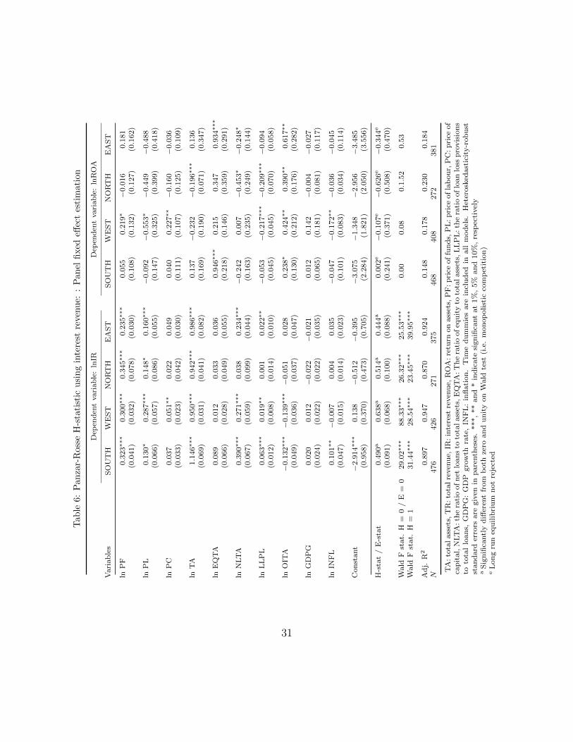
Tab

le6:

Pan

zar-

Ros

seH

-sta

tist

icu

sing

inte

rest

reven

ue:

:P

an

elfi

xed

effec

tes

tim

ati

on

Dep

end

ent

vari

ab

le:

lnIR

Dep

end

ent

vari

ab

le:

lnR

OA

Vari

ab

les

SO

UT

HW

ES

TN

OR

TH

EA

ST

SO

UT

HW

ES

TN

OR

TH

EA

ST

lnP

F0.3

23∗∗∗

0.3

00∗∗∗

0.3

45∗∗∗

0.2

35∗∗∗

0.0

55

0.2

19∗

−0.0

16

0.1

81

(0.0

41)

(0.0

32)

(0.0

78)

(0.0

30)

(0.1

08)

(0.1

32)

(0.1

27)

(0.1

62)

lnP

L0.1

30∗

0.2

87∗∗∗

0.1

48∗

0.1

60∗∗∗

−0.0

92

−0.5

53∗

−0.4

49

−0.4

88

(0.0

66)

(0.0

57)

(0.0

86)

(0.0

55)

(0.1

47)

(0.3

25)

(0.3

99)

(0.4

18)

lnP

C0.0

37

0.0

51∗∗

0.0

22

0.0

49

0.0

40

0.2

27∗∗

−0.1

60

−0.0

36

(0.0

33)

(0.0

23)

(0.0

42)

(0.0

30)

(0.1

11)

(0.1

07)

(0.1

25)

(0.1

09)

lnT

A1.1

46∗∗∗

0.9

50∗∗∗

0.9

42∗∗∗

0.9

86∗∗∗

0.1

37

−0.2

32

−0.1

96∗∗∗

0.1

36

(0.0

69)

(0.0

31)

(0.0

41)

(0.0

82)

(0.1

69)

(0.1

90)

(0.0

71)

(0.3

47)

lnE

QT

A0.0

89

0.0

12

0.0

33

0.0

36

0.9

46∗∗∗

0.2

15

0.3

47

0.9

34∗∗∗

(0.0

66)

(0.0

28)

(0.0

49)

(0.0

55)

(0.2

18)

(0.1

46)

(0.3

59)

(0.2

91)

lnN

LT

A0.3

90∗∗∗

0.2

71∗∗∗

0.0

38

0.2

34∗∗∗

−0.2

42

0.0

07

−0.4

53∗

−0.2

48∗

(0.0

67)

(0.0

59)

(0.0

99)

(0.0

44)

(0.1

63)

(0.2

35)

(0.2

49)

(0.1

44)

lnL

LP

L0.0

63∗∗∗

0.0

19∗∗

0.0

01

0.0

22∗∗

−0.0

53

−0.2

17∗∗∗

−0.2

09∗∗∗

−0.0

94

(0.0

12)

(0.0

08)

(0.0

14)

(0.0

10)

(0.0

45)

(0.0

45)

(0.0

70)

(0.0

58)

lnO

ITA

−0.1

32∗∗∗

−0.1

39∗∗∗

−0.0

51

0.0

28

0.2

38∗

0.4

24∗∗

0.3

90∗∗

0.6

17∗∗

(0.0

49)

(0.0

36)

(0.0

37)

(0.0

47)

(0.1

30)

(0.2

12)

(0.1

76)

(0.2

82)

lnG

DP

G0.0

20

0.0

12

−0.0

22

−0.0

21

0.0

12

0.1

42

−0.0

04

−0.0

27

(0.0

24)

(0.0

22)

(0.0

22)

(0.0

35)

(0.0

65)

(0.1

81)

(0.0

81)

(0.1

17)

lnIN

FL

0.1

01∗∗

−0.0

07

0.0

04

0.0

35

−0.0

47

−0.1

72∗∗

−0.0

36

−0.0

45

(0.0

47)

(0.0

15)

(0.0

14)

(0.0

23)

(0.1

01)

(0.0

83)

(0.0

34)

(0.1

14)

Con

stant

−2.9

14∗∗∗

0.1

38

−0.5

12

−0.3

95

−3.0

75

−1.3

48

−2.9

56

−3.4

85

(0.9

58)

(0.3

70)

(0.4

73)

(0.7

05)

(2.2

84)

(1.8

21)

(2.0

50)

(3.5

56)

H-s

tat

/E

-sta

t0.4

90a

0.6

38a

0.5

14a

0.4

44a

0.0

02e

−0.1

07e

−0.6

26e

−0.3

44e

(0.0

91)

(0.0

68)

(0.1

00)

(0.0

88)

(0.2

41)

(0.3

71)

(0.5

08)

(0.4

70)

Wald

Fst

at.

H=

0/

E=

029.0

2∗∗∗

88.3

3∗∗∗

26.3

2∗∗∗

25.5

3∗∗∗

0.0

00.0

80.1.5

20.5

3W

ald

Fst

at.

H=

131.4

4∗∗∗

28.5

4∗∗∗

23.4

5∗∗∗

39.9

5∗∗∗

Ad

j.R

20.8

97

0.9

47

0.8

70

0.9

24

0.1

48

0.1

78

0.2

30

0.1

84

N476

426

271

375

468

408

272

381

TA

:to

talass

ets,

TR

:to

talre

ven

ue,

IR:in

tere

stre

ven

ue,

RO

A:re

turn

on

ass

ets,

PF

:p

rice

of

fun

ds,

PL

:p

rice

of

lab

ou

r,P

C:p

rice

of

cap

ital,

NLT

A:th

era

tio

of

net

loan

sto

tota

lass

ets,

EQ

TA

:T

he

rati

oof

equ

ity

toto

talass

ets,

LL

PL

:th

era

tio

of

loan

loss

pro

vis

ion

sto

tota

llo

an

s,G

DP

G:

GD

Pgro

wth

rate

,IN

FL

:in

flati

on

.T

ime

du

mm

ies

are

incl

ud

edin

all

mod

els.

Het

erosk

edast

icit

y-r

ob

ust

stan

dard

erro

rsare

giv

enin

pare

nth

eses

.***,

**

an

d*

ind

icate

signifi

cant

at

1%

,5%

an

d10%

,re

spec

tivel

ya

Sig

nifi

cantl

yd

iffer

ent

from

both

zero

an

du

nit

yon

Wald

test

(i.e

.m

on

op

olist

icco

mp

etit

ion

)e

Lon

gru

neq

uilib

riu

mn

ot

reje

cted

31

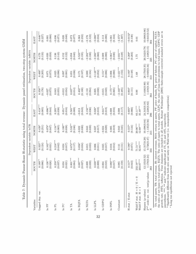
Tab

le7:

Dyn

amic

Pan

zar-

Ros

seH

-sta

tist

icu

sin

gto

tal

reven

ue:

Dyn

am

icp

an

eles

tim

ati

on

,tw

o-s

tep

syst

emG

MM

Dep

end

ent

vari

ab

le:

lnT

RD

epen

den

tvari

ab

le:

lnR

OA

Vari

ab

les

SO

UT

HW

ES

TN

OR

TH

EA

ST

SO

UT

HW

ES

TN

OR

TH

EA

ST

Lagged

dep

.var.

0.1

89∗∗

0.3

23∗∗

0.4

39∗

0.4

18∗∗∗

0.3

50∗∗

0.4

00∗

0.1

70

0.6

46∗∗∗

(0.0

86)

(0.1

24)

(0.2

51)

(0.0

85)

(0.1

76)

(0.2

05)

(0.1

33)

(0.2

27)

lnP

F0.1

26∗∗∗

0.1

62∗∗∗

0.0

79∗

0.0

96∗∗

−0.0

27

0.0

71

−0.0

20

0.0

01

(0.0

26)

(0.0

31)

(0.0

47)

(0.0

44)

(0.0

75)

(0.0

75)

(0.0

59)

(0.0

88)

lnP

L0.2

59∗∗∗

0.2

18∗∗∗

0.1

34∗∗

0.2

05∗∗∗

0.0

43

0.0

25

0.1

36

−0.0

36

(0.0

37)

(0.0

42)

(0.0

65)

(0.0

38)

(0.0

55)

(0.0

96)

(0.1

43)

(0.0

71)

lnP

C0.0

34

0.0

24

0.1

00∗∗

0.0

51∗∗∗

−0.0

12

0.0

97

0.1

52

0.0

20

(0.0

21)

(0.0

17)

(0.0

38)

(0.0

16)

(0.0

34)

(0.0

81)

(0.1

22)

(0.0

48)

lnT

A0.8

01∗∗∗

0.6

72∗∗∗

0.5

32∗∗

0.5

85∗∗∗

0.0

37∗∗∗

0.0

51

−0.0

58

0.0

72

(0.0

84)

(0.1

17)

(0.2

46)

(0.0

89)

(0.0

14)

(0.0

36)

(0.0

40)

(0.0

77)

lnE

QT

A0.0

87∗∗∗

0.0

56∗

−0.0

22

−0.0

13

0.4

02∗∗∗

0.1

71

0.5

23∗∗∗

0.3

63

(0.0

27)

(0.0

34)

(0.0

30)

(0.0

43)

(0.1

00)

(0.1

07)

(0.1

95)

(0.2

32)

lnN

LT

A−

0.0

09

0.0

15

0.0

43

0.1

50∗∗∗

−0.1

10

0.0

89

−0.2

82∗∗∗

−0.1

76

(0.0

39)

(0.0

33)

(0.0

39)

(0.0

36)

(0.0

94)

(0.1

04)

(0.1

00)

(0.1

22)

lnL

LP

L0.0

39∗∗∗

0.0

06

0.0

27

0.0

20∗

0.0

05

−0.1

48∗∗∗

−0.2

00∗∗∗

−0.0

80∗∗

(0.0

09)

(0.0

11)

(0.0

17)

(0.0

10)

(0.0

30)

(0.0

52)

(0.0

60)

(0.0

34)

lnG

DP

G−

0.0

04

0.0

25

−0.0

24

0.0

41∗∗

−0.0

15

0.1

51∗

−0.0

09

0.1

13

(0.0

18)

(0.0

17)

(0.0

29)

(0.0

18)

(0.0

49)

(0.0

86)

(0.0

80)

(0.0

80)

lnIN

FL

0.0

80∗∗∗

0.0

16

0.0

05

−0.0

08

0.1

75∗∗∗

−0.0

06

−0.0

61∗∗

−0.0

61

(0.0

17)

(0.0

12)

(0.0

19)

(0.0

16)

(0.0

65)

(0.0

80)

(0.0

30)

(0.1

04)

Con

stant

0.0

85

0.1

41

0.0

43

0.0

08

−2.4

40∗∗∗

−3.4

21∗∗∗

−2.0

31∗∗∗

−2.3

75∗

(0.1

59)

(0.1

51)

(0.3

45)

(0.1

17)

(0.4

85)

(1.1

53)

(0.4

49)

(1.3

07)

H-s

tat

/E

-sta

t0.5

17a

0.5

96a

0.5

57a

0.6

05a

0.0

04e

0.1

93e

0.2

69e

−0.0

152e

(0.0

43)

(0.0

71)

(0.1

24)

(0.0

66)

(0.1

11)

(0.1

49)

(0.2

03)

(0.1

30)

Wald

Fst

at.

H=

0/

E=

0232.1

9∗∗∗

71.5

1∗∗∗

20.0

6∗∗∗

83.1

1∗∗∗

0.0

01.6

81.7

50.0

1W

ald

Fst

at.

H=

1203.0

7∗∗∗

32.8

1∗∗∗

12.6

8∗∗∗

35.4

9∗∗∗

Han

sen

(p-v

alu

es)

12.1

35(0.5

2)

15.3

17(0.2

9)

10.4

98(0.8

4)

24.3

43(0.1

8)

11.6

46(0.9

0)

28.1

70(0.3

5)

20.3

42(0.7

8)

10.0

88(0.8

6)

2nd

ord

erse

r.co

r.te

st(p

-valu

es1.1

78(0.2

4)

0.7

26(0.4

7)

−1.1

35(0.5

6)

0.2

28(0.8

2)

1.4

18(0.1

6)

−0.9

49(0.3

4)

1.4

48(0.1

5)

−0.6

41(0.5

2)

N383

334

215

296

364

313

225

304

TA

:to

tal

ass

ets,

TR

:to

tal

reven

ue,

IR:

inte

rest

reven

ue,

RO

A:

retu

rnon

ass

ets,

PF

:p

rice

of

fun

ds,

PL

:p

rice

of

lab

ou

r,P

C:

pri

ceof

cap

ital,

NLT

A:

the

rati

oof

net

loan

sto

tota

lass

ets,

EQ

TA

:T

he

rati

oof

equ

ity

toto

tal

ass

ets,

LL

PL

:th

era

tio

of

loan

loss

pro

vis

ion

sto

tota

llo

an

s,G

DP

G:

GD

Pgro

wth

rate

,IN

FL

:in

flati

on

.T

ime

du

mm

ies

are

incl

ud

edin

all

mod

els.

Rob

ust

Win

dm

eije

r(2

005)

fin

ite-

sam

ple

corr

ecte

dst

an

dard

erro

rsare

inp

are

nth

esis

.***,

**

an

d*

ind

icate

sign

ifica

nt

at

1%

,5%

an

d10%

,re

spec

tivel

ya

Sig

nifi

cantl

yd

iffer

ent

from

both

zero

an

du

nit

yon

Wald

test

(i.e

.m

on

op

olist

icco

mp

etit

ion

)e

Lon

gru

neq

uilib

riu

mn

ot

reje

cted

32

Tab

le8:

Dyn

amic

Pan

zar-

Ros

seH

-sta

tist

icu

sin

gth

era

tio

of

tota

lre

ven

ue

toto

tal

ass

ets:

Dyn

am

icp

anel

esti

mati

on

,tw

o-s

tep

syst

emG

MM

Dep

end

ent

vari

ab

le:

ln(T

R/T

A)

Dep

end

ent

vari

ab

le:

lnR

OA

Vari

ab

les

SO

UT

HW

ES

TN

OR

TH

EA

ST

SO

UT

HW

ES

TN

OR

TH

EA

ST

Lagged

dep

.var.

0.5

43∗∗

0.5

15∗∗

0.4

65∗

0.4

25∗∗∗

0.3

30∗∗

0.4

17∗∗

0.8

79∗∗∗

0.6

49∗∗

(0.2

22)

(0.2

53)

(0.2

46)

(0.1

10)

(0.1

47)

(0.2

10)

(0.1

75)

(0.2

48)

lnP

F0.0

86∗∗∗

0.1

32∗∗∗

0.1

03∗∗∗

0.0

73∗∗∗

−0.0

07

0.0

81

−0.0

57

−0.0

52

(0.0

29)

(0.0

43)

(0.0

33)

(0.0

25)

(0.0

75)

(0.0

73)

(0.0

83)

(0.0

94)

lnP

L0.1

61∗

0.1

89∗∗∗

0.1

37∗

0.2

19∗∗∗

0.0

33

−0.0

29

−0.0

60

−0.0

69

(0.0

86)

(0.0

65)

(0.0

74)

(0.0

51)

(0.0

54)

(0.0

84)

(0.1

20)

(0.0

90)

lnP

C0.0

25

0.0

17

0.1

14∗∗∗

0.0

61∗∗∗

−0.0

14

0.0

83

−0.0

84

−0.0

02

(0.0

19)

(0.0

17)

(0.0

35)

(0.0

18)

(0.0

35)

(0.0

77)

(0.0

97)

(0.0

50)

lnE

QT

A0.0

74∗∗

0.0

48

0.0

19

−0.0

09

0.3

66∗∗∗

0.1

70

0.1

49

0.2

90

(0.0

36)

(0.0

34)

(0.0

28)

(0.0

28)

(0.0

87)

(0.1

09)

(0.1

51)

(0.1

85)

lnN

LT

A0.0

44

0.1

31∗∗

0.0

19

0.1

60∗∗∗

−0.0

75

0.0

65

−0.1

26

−0.1

70

(0.0

32)

(0.0

57)

(0.0

43)

(0.0

35)

(0.0

88)

(0.1

04)

(0.1

01)

(0.1

19)

lnL

LP

L0.0

40∗∗∗

0.0

13

0.0

43∗∗∗

0.0

28∗∗∗

0.0

15

−0.1

51∗∗∗

−0.1

25∗

−0.0

80∗∗

(0.0

11)

(0.0

10)

(0.0

15)

(0.0

08)

(0.0

31)

(0.0

52)

(0.0

71)

(0.0

38)

lnG

DP

G−

0.0

23

0.0

32∗

−0.0

31

0.0

44∗∗

−0.0

11

0.1

52∗

0.2

18

0.1

06

(0.0

17)

(0.0

17)

(0.0

21)

(0.0

18)

(0.0

50)

(0.0

86)

(0.2

26)

(0.0

85)

lnIN

FL

0.0

82∗∗∗

0.0

09

0.0

01

0.0

01

0.1

72∗∗∗

−0.0

05

−0.1

07

−0.0

34

(0.0

24)

(0.0

14)

(0.0

12)

(0.0

18)

(0.0

64)

(0.0

84)

(0.0

70)

(0.0

96)

Con

stant

0.2

06∗

0.3

52∗∗

−0.0

63

−0.0

02

−2.0

10∗∗∗

−2.8

90∗∗∗

−1.4

26∗∗

−1.9

56∗

(0.1

08)

(0.1

75)

(0.2

51)

(0.1

13)

(0.3

59)

(1.0

38)

(0.6

40)

(1.0

49)

H-s

tat

/E

-sta

t0.5

95a

0.6

95a

0.6

61a

0.6

15a

0.0

12e

0.1

35e

−0.2

02e

−0.1

22e

(0.0

43)

(0.1

62)

(0.1

30)

(0.0

47)

(0.1

11)

(0.1

31)

(0.2

32)

(0.1

66)

Wald

Fst

at.

H=

0/

E=

057.0

5∗∗∗

18.2

9∗∗∗

25.9

5∗∗∗

172.1

8∗∗∗

0.0

11.0

60.7

50.5

4W

ald

Fst

at.

H=

126.4

2∗∗∗

3.5

2∗

6.8

0∗∗

67.4

3∗∗∗

Han

sen

Jte

st(p

-valu

es)

16.5

84(0.2

2)

12.2

26(0.5

1)

0.1

15(0.7

3)

0.0

81(0.7

8)

11.6

69(0.9

0)

28.2

36(0.3

5)

0.1

36(0.7

1)

11.0

59(0.8

1)

2nd

ord

erse

r.co

r.te

st(p

-valu

es)

0.9

36(0.3

5)

1.4

58(0.1

5)

−0.4

38(0.6

6)

0.3

35(0.7

4)

1.4

18(0.1

6)

−1.0

02(0.3

2)

1.5

58(0.1

2)

−0.5

37(0.5

9)

N383

334

215

296

364

313

225

304

TA

:to

tal

ass

ets,

TR

:to

tal

reven

ue,

IR:

inte

rest

reven

ue,

RO

A:

retu

rnon

ass

ets,

PF

:pri

ceof

fun

ds,

PL

:p

rice

of

lab

ou

r,P

C:

pri

ceof

cap

ital,

NLT

A:

the

rati

oof

net

loan

sto

tota

lass

ets,

EQ

TA

:T

he

rati

oof

equ

ity

toto

tal

ass

ets,

LL

PL

:th

era

tio

of

loan

loss

pro

vis

ion

sto

tota

llo

an

s,G

DP

G:

GD

Pgro

wth

rate

,IN

FL

:in

flati

on

.T

ime

du

mm

ies

are

incl

ud

edin

all

mod

els.

Rob

ust

Win

dm

eije

r(2

005)

fin

ite-

sam

ple

corr

ecte

dst

an

dard

erro

rsare

inp

are

nth

esis

.***,

**

an

d*

ind

icate

sign

ifica

nt

at

1%

,5%

an

d10%

,re

spec

tivel

ya

Sig

nifi

cantl

yd

iffer

ent

from

both

zero

an

du

nit

yon

Wald

test

(i.e

.m

on

op

olist

icco

mp

etit

ion

)e

Lon

gru

neq

uilib

riu

mn

ot

reje

cted

33

Tab

le9:

Dyn

amic

Pan

zar-

Ros

seH

-sta

tist

icu

sin

gto

tal

reven

ue:

Dyn

am

icp

an

eles

tim

ati

on

,tw

o-s

tep

syst

emG

MM

Dep

end

ent

vari

ab

le:

lnIR

Dep

end

ent

vari

ab

le:

lnR

OA

Vari

ab

les

SO

UT

HW

ES

TN

OR

TH

EA

ST

SO

UT

HW

ES

TN

OR

TH

EA

ST

Lagged

dep

.var.

0.2

37∗∗

0.3

25∗∗∗

0.5

81∗∗∗

0.5

61∗∗∗

0.3

62

0.4

23∗∗

0.3

03∗

0.5

58∗∗

(0.1

02)

(0.0

99)

(0.1

92)

(0.1

78)

(0.2

22)

(0.1

70)

(0.1

62)

(0.2

38)

lnP

F0.2

20∗∗∗

0.2

67∗∗∗

0.0

68

0.1

33∗∗∗

0.0

03

0.1

01

0.0

21

0.0

70

(0.0

37)

(0.0

29)

(0.0

50)

(0.0

44)

(0.0

82)

(0.0

62)

(0.0

41)

(0.1

06)

lnP

L0.2

05∗∗∗

0.2

43∗∗∗

0.1

43∗

0.1

60∗∗

−0.1

37∗

−0.0

55

−0.0

77

−0.1

00

(0.0

39)

(0.0

44)

(0.0

76)

(0.0

79)

(0.0

80)

(0.1

17)

(0.1

37)

(0.1

07)

lnP

C−

0.0

06

0.0

37∗∗∗

0.0

12

0.0

49∗∗

−0.0

01

0.1

79∗∗

−0.0

41

0.0

30

(0.0

25)

(0.0

13)

(0.0

38)

(0.0

20)

(0.0

35)

(0.0

79)

(0.0

80)

(0.0

55)

lnT

A0.7

51∗∗∗

0.6

80∗∗∗

0.3

83∗∗

0.4

50∗∗∗

0.0

22

0.0

40

−0.0

90∗∗

0.1

21

(0.1

01)

(0.0

89)

(0.1

89)

(0.1

71)

(0.0

15)

(0.0

36)

(0.0

37)

(0.0

78)

lnE

QT

A0.0

48

0.0

23

−0.0

54

−0.0

27

0.3

97∗∗∗

0.1

51

0.3

78∗∗∗

0.4

71∗

(0.0

42)

(0.0

24)

(0.0

43)

(0.0

48)

(0.1

10)

(0.0

92)

(0.1

30)

(0.2

50)

lnN

LT

A0.0

12

0.0

87

0.0

42

0.2

24∗∗∗

−0.0

55

0.0

98

−0.1

43∗

−0.1

67

(0.0

53)

(0.0

64)

(0.0

53)

(0.0

43)

(0.0

74)

(0.1

04)

(0.0

73)

(0.1

44)

lnL

LP

L0.0

16

0.0

05

0.0

05

0.0

08

−0.0

08

−0.1

07∗∗

−0.1

61∗∗∗

−0.1

02∗∗

(0.0

12)

(0.0

12)

(0.0

18)

(0.0

14)

(0.0

37)

(0.0

46)

(0.0

44)

(0.0

42)

lnO

ITA

−0.0

51∗

−0.0

79∗

−0.0

45∗

−0.0

46

0.1

99∗

0.3

53∗∗

0.0

60

0.1

43

(0.0

29)

(0.0

40)

(0.0

25)

(0.0

30)

(0.1

00)

(0.1

71)

(0.0

44)

(0.1

41)

lnG

DP

G0.0

51∗

0.0

86∗∗∗

−0.0

24

0.0

42

0.0

23

0.1

22

−0.0

15

0.0

87

(0.0

26)

(0.0

24)

(0.0

22)

(0.0

28)

(0.0

55)

(0.0

96)

(0.0

74)

(0.0

86)

lnIN

FL

0.0

99∗∗∗

0.0

14

−0.0

07

−0.0

18

0.1

50∗

−0.0

39

−0.0

46

−0.0

42

(0.0

29)

(0.0

14)

(0.0

14)

(0.0

25)

(0.0

76)

(0.0

69)

(0.0

30)

(0.0

89)

Con

stant

−0.4

23∗∗

−0.1

41

−0.0

43

−0.1

18

−2.1

46∗∗∗

−2.0

80∗

−1.7

29∗∗∗

−2.6

50∗

(0.1

88)

(0.2

60)

(0.4

30)

(0.1

62)

(0.4

61)

(1.1

48)

(0.5

59)

(1.3

41)

H-s

tat

/E

-sta

t0.5

50a

0.8

10a

0.5

34a

0.7

80a

−0.1

35e

0.2

25e

−0.0

97e

0.0

01e

(0.0

58)

(0.0

78)

(0.1

93)

(0.1

00)

(0.1

20)

(0.1

42)

(0.1

68)

(0.1

57)

Wald

Fst

at.

H=

0/

E=

090.9

1∗∗∗

108.8

3∗∗∗

7.6

7∗∗∗

61.2

3∗∗∗

1.2

52.4

90.3

30.0

0W

ald

Fst

at.

H=

160.7

2∗∗∗

5.9

5∗∗

5.8

5∗∗

4.8

8∗∗

Han

sen

test

(p-v

alu

es)

21.5

86(0.1

6)

12.2

95(0.5

0)

32.0

98(0.1

9)

27.6

07(0.1

2)

7.7

26(0.8

6)

16.3

15(0.4

39.2

74(0.9

0)

19.5

34(0.4

8)

Sec

on

dord

erse

r.co

r.te

st(p

-valu

es)

0.1

93(0.8

5)

0.5

61(0.5

8)

1.3

73(0.1

7)

0.2

54(0.8

0)

0.9

71(0.3

3)

−0.6

77(0.5

0)

1.2

56(0.2

1)

−0.5

41(0.5

9)

N374

334

206

297

354

311

212

301

TA

:to

tal

ass

ets,

TR

:to

tal

reven

ue,

IR:

inte

rest

reven

ue,

RO

A:

retu

rnon

ass

ets,

PF

:p

rice

of

fun

ds,

PL

:p

rice

of

lab

ou

r,P

C:

pri

ceof

cap

ital,

NLT

A:

the

rati

oof

net

loan

sto

tota

lass

ets,

EQ

TA

:T

he

rati

oof

equ

ity

toto

tal

ass

ets,

LL

PL

:th

era

tio

of

loan

loss

pro

vis

ion

sto

tota

llo

an

s,G

DP

G:

GD

Pgro

wth

rate

,IN

FL

:in

flati

on

.T

ime

du

mm

ies

are

incl

ud

edin

all

mod

els.

Rob

ust

Win

dm

eije

r(2

005)

fin

ite-

sam

ple

corr

ecte

dst

an

dard

erro

rsare

inp

are

nth

esis

.***,

**

an

d*

ind

icate

sign

ifica

nt

at

1%

,5%

an

d10%

,re

spec

tivel

ya

Sig

nifi

cantl

yd

iffer

ent

from

both

zero

an

du

nit

yon

Wald

test

(i.e

.m

on

op

olist

icco

mp

etit

ion

)e

Lon

gru

neq

uilib

riu

mn

ot

reje

cted

34