
Bank risk taking, efficiency, and legal environment: from Chinese
36
1 Bank risk taking, efficiency, and legal environment: Evidence from Chinese banks Jianhua Zhang Peng Wang People’s Bank of China China Baozhi Qu Department of Economics and Finance City University of Hong Kong Hong Kong E-mail: [email protected] Phone: 00-852-3442-7312 Fax: 00-852-3442-0284 This version: September 10, 2010
Transcript of Bank risk taking, efficiency, and legal environment: from Chinese

1
Bank risk taking, efficiency, and legal environment:
Evidence from Chinese banks
Jianhua Zhang Peng Wang
People’s Bank of China China
Baozhi Qu Department of Economics and Finance
City University of Hong Kong Hong Kong
E-mail: [email protected] Phone: 00-852-3442-7312
Fax: 00-852-3442-0284
This version: September 10, 2010
2
Bank risk taking, efficiency, and legal environment:
Evidence from Chinese banks
Abstract
We investigate bank risk taking, efficiency and their relation to legal environment using a unique sample of 133 Chinese banks across 31 regions for the 1999-2008 period. We find that stronger legal protection tends to promote greater bank risk taking in the region. Furthermore, employing a stochastic distance function approach, our analysis shows that the performance of Chinese banks, as measured by bank efficiency, is heavily influenced by the legal environment in the region. More developed market intermediaries, higher efficiency in the legal system, and better protection of intellectual property right are associated with a higher level of efficiency among these banks.
JEL Classification:G01, G21, G28 Keywords: Bank risk taking; Bank efficiency; Legal environment; Stochastic frontier
analysis; China

3
1. Introduction
The growing law and finance literature (pioneered by La Porta et al., 1998) has
documented that a well-developed legal environment enhance the enforcement of financial
contracts. Since banks are usually in the center of a country’s financial system and their
operation and performance depend heavily on the contract enforcement (e.g., a loan contract),
legal environment may have a significant impact on banking. Previous research has reported
evidence of such influences. For instance, Cole and Turk-Ariss (2008) find that banks have
higher loan ratios in countries with English legal origin and weaker creditor rights. Houston et
al. (2010) document that stronger creditor rights tend to promote greater bank risk taking. The
legal environment may also influence the operation and performance of a country’s
banking sector through other channels, such as by enhancing lending technology
(Berger and Udell, 2006), increased availability of loans (Qian and Strahan, 2007), or
reduced rigidity of regulations (Demirguc-Kunt et al., 2003).
Noticeably absent in this area is a direct examination of the potential effects of the legal
environment on bank performance (Berger and Mester, 1997; Hasan et al., 2009). In addition,
most of the abovementioned studies use a standard cross-country setting. However, various
studies have found a significant degree of variation in the institutional and legal environment
within a particular country and such variation may be important in affecting economic
outcomes.1 Micro data analysis at the bank level that takes into consideration the variation in
1For instance, corruption in some regions may be more pervasive than that in other regions, and a country may have strong rules and regulations on the books but weak law enforcement in some regions and for some firms. Berkowitz and Clay (2006) show that the quality of state courts varies significantly across U.S. states and is greatly affected by the initial conditions of a state. Laeven and Woodruff (2007) find significant variation in the quality of the Mexican legal system. Acemoglu and Dell (2009) argue that both de jure and de facto institutions vary greatly within countries. Using World Bank enterprise survey data, Ma et al. (2009) find that the average within-country variation in judicial quality is much greater than the cross-country variation in judicial quality.

4
institutional quality within a country can therefore provide valuable empirical evidence that
complements and extends the existing country-level research. As Acemoglu (2005) correctly
points out, questions related to the importance of legal institutions “will be almost impossible
to answer with cross-country data alone, and micro data investigations, for example,
exploiting differences in regulations across markets and regions appear to be a most
promising avenue” (p. 1045).
Our study contributes to the literature by providing bank-level evidence of a link between
bank risk taking, bank performance (measured by bank efficiency), and the legal environment
using a within-country setting. We focus on within-country effects of regional institutions on
bank risk taking and performance by taking into account the striking heterogeneity of
bank-level characteristics. We take advantage of a unique data set which has extensive
information on 133 Chinese city commercial banks (CCBs) from 1999-2008. Such a rich data
set of Chinese CCBs serves our purpose particularly well because China is a big country with
great regional variation. Although China is a centralized country so that the laws on
book are highly uniform across regions, the quality of law enforcement varies
significantly across provinces. CCBs usually conduct their business only within the
boundaries of a city or province, which provides us with a unique opportunity to study how
regional institutional environment affect bank risk taking and performance while controlling
for a large set of bank-level characteristics and country-level variables2.
We examine two questions about Chinese banks: First, how does the legal
environment affect bank risk taking? Second, how is bank efficiency associated with the
2 This empirical setting distances our paper from similar research (e.g., Hasan et al. 2009) that focuses on Chinese banks that have country-wide banking operation. If a bank is allowed to operate across different provinces, then it will be difficult to isolate the effect of regional institutional environment on its efficiency.
5
legal environment of the region? In China, significant market-oriented reforms took
place during the past decade and these reforms led to important changes in the legal
environment of Chinese banks.3 These changes developed in a very unbalanced way
across different provinces, especially in terms of the effectiveness of law enforcement.
According to Fan and Wong’s (2010) measures, the necessary market intermediaries
that are essential for the effective law enforcement are more developed in some
provinces (such as Zhejiang) than others (such as Qinghai). Similarly, the efficiency
of the regional legal system and the protection of the intellectual property rights also
have great variations across provinces. Such difference in law enforcement could
affect bank risk taking and the efficiency of banks in the region both directly and
indirectly. For instance, more effective law enforcement reduces credit risk by
providing more protection to banks when the loan contract is defaulted, thus
encourage banks to take more risks and make more loans (Houston et al., 2010). In
addition, better legal protection (such as protection of the intellectual rights) creates a
better market environment for firms thus may improve the performance of borrowers.
This will in turn affect banks indirectly by reducing the credit risk of banks’ loan
portfolio and encourage banks to take more risk by lending to more risky borrowers
such as new startups of IT companies.
Our empirical results show that stronger legal protection encourages risk taking among
Chinese banks, which is consistent with the cross-country research by Houston et al. (2010).
In addition, using a stochastic function approach, our study shows that better developed
3 Given that the banking sector in China has been under heavy regulation of the government and most of the reforms related to this sector followed a “top-down” procedure, we expect that the causality goes from market development and institutional changes to banks’ profit efficiency and not the other way around.

6
market intermediaries, more efficient law enforcement and better protection of intellectual
property rights are significantly related to greater bank efficiency.
The rest of the paper is organized as follows. The next section explains the institutional
background of the Chinese banking sector and the development of CCBs. Section 3 describes
the estimation procedure and data. Section 4 reports the empirical results, and section 5
concludes the paper.
2. The development of CCBs in China
The Chinese banking system has gone through significant transformation since 1978.
The all-in-one mono-bank system under the planned was replaced by a banking sector
dominated by the four state-owned specialized banks (the Big Four, i.e., the Agricultural Bank
of China, Bank of China, China Construction Bank and Industrial and Commercial Bank of
China) during 1979-1993. The Big Four were further transformed into state-owned
commercial banks during 1994-97 and partially privatized by getting listed on the Shanghai
and Hong Kong stock exchanges during 2005-2010 after receiving several rounds of capital
injection since 1997. In addition to the Big Four who dominated China’s financial landscape,
there are quite a number of joint-stock commercial banks (JSCBs), CCBs and other types of
financial institutions operating in the banking sector. In addition, a number of foreign banks
have been allowed to operate in China with full banking licenses since 2006. As of the end of
2008, the total assets of the Chinese banking sector amounted to RMB62.4 trillion. The Big
Four, the JSCBs, and the CCBs held 71.8% of the total assets (51% by the Big Four,
13.1% by the JSCBs, and 6.6% by CCBs).

7
CCBs emerged in China only in 1995. On 7 September 1995, the State Council issued
Guidelines of the Establishment of the City Cooperative Bank. City cooperative banks (the
precursors of CCBs) were set up in 35 medium- and large-sized cities. The first generation of
CCBs were formed through the merging of 2194 urban credit cooperatives, rural credit
cooperatives and local financial service institutions. Hence, CCBs were also regarded as
JSCBs at the time. Similar banks were later established in other cities. By 2008, the number
of CCBs had increased, with at least one CCB in almost every major city. However, these
banks are unevenly distributed, with more branches in the economically more developed
eastern provinces (such as Guangdong) than in the less developed western provinces (such as
Qinghai). By regulation, CCBs can provide financial services only in their own administrative
region. Therefore, a typical CCB is much smaller than a Big Four bank. For instance, the
amount of total loans per CCB was RMB6,219 million in 2008 (2000 price level), compared
to RMB1,841,047 million for a Big Four bank and RMB173,869 million for a JSCB. Table 1
presents the summary statistics of the basic financial ratios for CCBs used in our analysis.
[Table 1 here]
In addition, CCBs differ from the Big Four in that the former have more diversified
shareholders from different classes in society, including individuals, private enterprises,
institutional investors, state-owned enterprises and the treasury of local governments. On
average, only about one-fourth of CCB shares are held directly by SOEs. Hence, CCBs are
subject to less state intervention and may have relatively better corporate governance
compared to the Big Four (Ferri, 2009). Using survey data on 20 CCBs from three provinces,
Ferri (2009) studies the performance of these banks, finding that they outperform the Big

8
Four and that geographic location significantly affects CCB performance and business. It is
also found that the degree of state intervention influences CCB corporate governance and
performance levels. Our study differs from that of Ferri (2009) in several ways: our data set
covers a much larger sample of CCBs across 31 provinces of the country, and we use a
distance function approach to study the efficiency of CCBs, which may better capture the
quality of banking institutions and their functions in the economy (Hasan et al., 2009). We
also pinpoint regional factors that affect the risk-taking and efficiency of CCBs and focus on
the difference in institutional quality across regions.
By focusing on CCBs in China, our paper makes a contribution to the efficiency study of
Chinese banks. A number of studies have examined bank efficiency in China (e.g., Jiang et al.,
2009; Hasan et al., 2009; Berger et al., 2009; Chen, 2005). Most of these studies focus on the
the Big Four and JSCBs that are relatively large with nationwide business operations,
probably because the financial information of these banks is publicly available and thus easily
obtained. However, one of the most important changes in the Chinese banking sector in the
past decade or so is the emergence and rapid development of a new breed of dynamic regional
banks – CCBs. In contrast to the traditional Big Four, these banks are recent entities, have a
lower level of state ownership and operate mainly in the regional market of a city or province.
As of 2008, there were more than 136 CCBs in China, with at least one in almost every major
city. Most of them, however, are unlisted. This constraint on data availability makes CCBs
significantly underrepresented in previous efficiency studies of Chinese banks. The very few
studies of CCBs have had to rely mainly on survey data, and their sample size is significantly
limited (e.g., Ferri, 2009). The rich data set of Chinese CCBs in our study thus allows us to

9
fill the gap by providing empirical evidence on the efficiency of CCBs and its determinants.
3. Data and model
3.1 Sample and measure of legal environment
Our data set was obtained from the PBC. It includes extensive information on 133
Chinese CCBs, including listed and unlisted banks, over 10 years (1999-2008). After deleting
some observations with incomplete data, we have a sample of 1083 observations. Table 2
shows the sample distribution over time.
[Table 2 here]
We rely on the various issues of the Market Development Report of Fan and Wang (2000,
2004, 2006 and 2010) to obtain measures of legal environment in 31 provinces. The reports
publish annual information about an index that measures the development of market
intermediaries and legal environment across different provinces from 1998-2007 and are
widely used in the literature. The development of market intermediaries measures the number
of lawyers and certified public accountants in relative to the population in the region. Higher
ratio of these professionals to the population indicates more effective law enforcement in the
region. We also look at two other variables that measure different aspects of law enforcement
in a province. The first variable concerns the efficiency of law enforcement, and it is based on
survey results of firms. A high value in this variable indicates higher efficiency level of local
law authority, as perceived by surveyed firms in the region. The second variable involves the
protection of intellectual property rights. A high value in this variable implies stronger legal

10
protection of intellectual property rights. In China, laws to protect intellectual property rights
are often insufficiently enforced deliberately by local governments to promote the regional
economy, and thus a strong protection of intellectual property rights can be taken as a symbol
of whether the region has a legal system that is less subject to interventions of local
government and local interest groups.
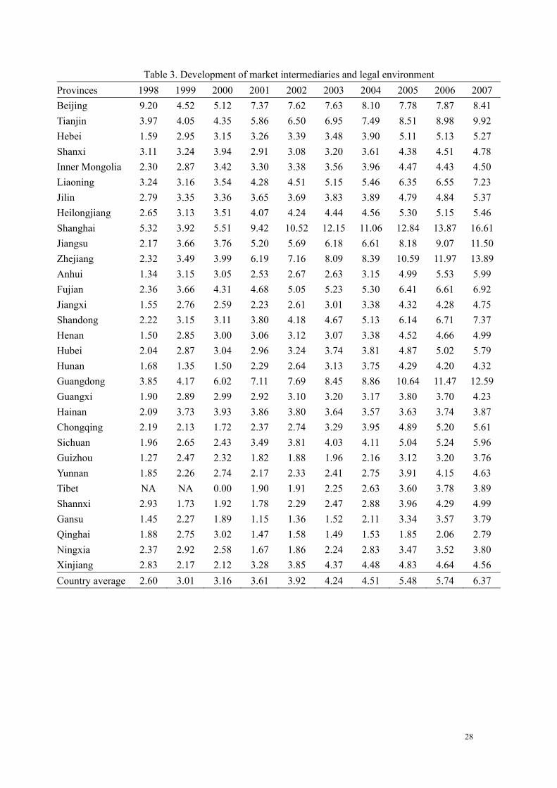
Table 3 presents the index of the development of market intermediaries and the legal
environment. The index shows significant variation both across regions and over time. The
effects of legal protection on bank risk taking and efficiency are likely to be lagged.
Consequently, we use the value of the measures of legal protection of the previous year in the
analysis. Our results are not sensitive to how the lagged effects are taken into account in the
regressions.
[Table 3 here]
3.2 Bank risk taking
As a measure of bank risk taking, we use the natural logarithm of the Z-score which is
the number of standard deviations that a bank’s rate return of assets has to fall for the bank to
become insolvent. The Z-score has been widely used in the recent literature (e.g., Laeven and
Levine, 2009; Demirguc-Kunt and Huizinga, 2009; Houston et al., 2010). Specifically,
Z-score = (ROA+CAR)/σ(ROA), where ROA is the mean rate of return on assets and CAR is
the mean equity-to-assets ratio. σ(ROA) is the standard deviation of ROA. Higher Z-score
implies more stability. We calculate a Z-score for a bank over time based on annual
accounting data for the past five years. Following Laeven and Levine (2009) and Houston et

11
al. (2010), we use the natural logarithm of the Z-score in the regressions to smooth out the
skewness of the Z-score.
To examine the impact that legal environment has on bank risk taking, we implement the
following fixed-effects estimation model:
Zijt = α + β1Legal Environment Measuresjt + β2Macro Controlsjt + β3Bank Controlsit +
β4Bank Fixed Effecti + β5Time Variablet + ε (1)
The dependent variable is the log Z-score, and the key independent variable is the
measure for the legal environment in the region. We also control for other macro variables at
the provincial level: the degree of financial deepening, measured by the ratio of total loans to
GDP of the province; scale of the economy, measured by the natural logarithm of gross
domestic product (GDP) at the beginning of the year (the GDP value is adjusted to the 2000
price level using the GDP deflator); and economic growth, measured by the annual GDP
growth rate. Following previous literature (e.g., Houston et al., 2010), we include a large set
of bank level control variables in the regressions: bank size and its quadratic form, growth
rate of the operating income, non-interest income to operating income ratio, equity to assets
ratio, interbank funds to interbank funds plus deposits ratio, non-performing loans (NPLs)
ratio, ratio of securities to total earnings assets, and a dummy variable for dynamic
governance change in the bank (IPO or the introduction of foreign investors). In addition, we
control for firm-fixed effects and time effect in the regressions. The measure of legal
environment and other macro variables are both time (t) and region (j) variables while the
bank control variables are bank specific variables (i) that vary over time.

12
3.3 Bank efficiency: the distance function approach
A stochastic frontier approach is commonly employed for efficiency analysis. Fries and
Taci (2005) argue that such an approach is appropriate in efficiency studies of transition
economies, in which problems related to measurement error and an uncertain economic
environment are more likely to prevail. Following previous studies (e.g., Wang and Schmidt,
2002; Jiang et al., 2009), we adopt the estimation procedure proposed by Battese and Coelli
(1995). The output distance function4 is defined as: { }0 ( , ) min : ( / ) ( )D x y y P xθ θ= ∈ .
Following Lovell et al. (1994), 0 ( , )D x y is non-decreasing, positively homogeneous and
convex in the output vector y and non-increasing in the input vector x . If y falls inside
the production possibility set ( )P x , then 0 ( , )D x y is less than one. If y falls on the
boundary of the production possibility set, then 0 ( , )D x y is equal to one. More specifically,
for a firm producing m outputs using n inputs, an output distance function in a
translog form is usually given by (e.g., Jiang et al., 2009):
01 1 1 1 1 1
1 1ln ( , , ) ln ln ln ln ln ln2 2
n m n n m mt t t t t t t t
o k k j j kh k h jl j lk j k h j l
D x y t x y x x y yα α β α β= = = = = =
= + + + +∑ ∑ ∑∑ ∑∑
2
1 1 1 1
1ln ln ln ln2
n m n mt t t t
kj k j t tt kt k jt jk j k j
x y t t x t y tγ ϕ ϕ ξ τ= = = =
+ + + + +∑∑ ∑ ∑ , (2)
where x is input, y is output (multiple inputs, multiple outputs) and t is time. As
( , , )t toD x y t is homogeneous of degree 1 in y , we obtain the following constraints:
11
m
jjβ
=
=∑ , 1
0( 1,2,.... )m
jll
j Mβ=
= =∑ , 1
0( 1, 2,.... )m
kjj
k Nγ=
= =∑ ,
10( 1, 2,.... )
m
jtj
j Mτ=
= =∑ , jl ljβ β= and kh hkα α= .
4A major advantage of the distance function approach is that it can be applied in the case of multiple inputs, multiple outputs or absence of price information when the traditional dual approach is inapplicable (Jiang et al., 2009).

13
Under these constraints, we can derive the following equation for individual firm i :
1*
01 1 1 1
1ln ln ln ln( ) ln ln2oi
n m n nt t t t t t
mi k ki j ji kh ki hik j k h
D y x y x xα α β α−
= = = =
− = + + +∑ ∑ ∑∑
1 1 1
* * * 2
1 1 1 1
1 1ln( ) ln( ) ln ln( )2 2
m m n mt t t t
jl ji li kj ki ji t ttj l k j
y y x y t tβ γ ϕ ϕ− − −
= = = =
+ + + +∑∑ ∑∑
1*
1 1ln ln( )
n mt t t
kt ki jt ji ik j
x t y t vξ τ−
= =
+ + +∑ ∑ , (3)
where *( ) / ( 1, 2,... 1)t t tji ji miy y y j m= = − . By definition, ln 0
oi
tD ≤ . We further define
lnoi
t tiu D= − : i.e., t
iu follows a non-negative truncated normal distribution. In addition,
2~ (0, )ti vv N σ : i.e., t
iv follows a standard normal distribution. tiu and t
iv are
independent. This is the standard setting of a stochastic frontier model.5
Following Battese and Coelli (1995), we further analyze the determinants of tiu . The
inefficiencies ( tiu ) can be further decomposed as t t t
i i iu z eδ= + , where tiz denotes the
exogenous factors that affect the technical inefficiency term, δ denotes the coefficients of
these factors and tie is a random variable, which is independently distributed as truncations
of a normal distribution 2(0, )uN σ (here, t ti ie z δ≥ − ). This means that t
iu is independently
distributed as non-negative truncations of a normal distribution 2( , )ti uN μ σ , in which
t ti izμ δ= , indicating that t
iμ , the expected value of tiu , is influenced by different factors
with a constant variance.
How to define and measure the inputs and outputs of a bank is an important issue in the
bank efficiency research. The two basic methods are the production and the intermediation
approach. Following the previous literature (e.g., Jiang et al. 2009), we use the latter6 and
5Simultaneous equation bias may exist when both inputs and outputs are included in the distance function as regressors. After the normalization procedure, output ratios may be treated as exogenous (Coelli and Perelman, 1996). 6Berger and Humphrey (1997) argue that under the production approach, financial institutions are thought of as
14
implement two different models: the first is an income-based model and the second is an
earning assets-based model. The definitions of the input and output factors included in these
two models are presented in Table 4.
[Table 4 here]
Following previous studies (e.g., Fu and Heffernan, 2007; Jiang et al., 2009), factors in
the analysis of technical efficiency are divided into macro factors and bank-level
characteristics as listed below. The main macro factor of interest is the measure of legal
environment of the region. Other macro factors include: the degree of financial deepening,
measured by the ratio of total loans to GDP of the province; scale of the economy, measured
by the natural logarithm of gross domestic product (GDP) at the beginning of the year (the
GDP value is adjusted to the 2000 price level using the GDP deflator); and economic growth,
measured by the annual GDP growth rate of the previous year. In addition, we consider a
large set of bank characteristics in the inefficiency analysis.
Governance variables. First, we include a dummy variable that measures the
selection governance of a bank (Berger et al., 2005), which takes the value of one if
the bank has foreign investors as big shareholders or is listed in a financial market
(including both domestic and oversea stock exchanges) during the sample period, and
primarily carrying out services for account holders. These institutions perform transactions and process documents for customers, including loan applications, credit reports, checks and other payment services, and insurance services. Under this approach, output is best measured by the number and type of transactions or documents processed over a given period. Unfortunately, such detailed transaction flow data are typically proprietary and not publically available. As a result, data on the stock of the number of deposit or loan accounts serviced or insurance policies outstanding are used instead. Also, only physical inputs such as physical capital, labor and their cost as well as operating expenses (excluding interest expenses) are used. In contrast, under the intermediation approach, financial institutions are thought of as primarily intermediating funds between savers and investors. Because service flow data are not usually available, the flows are typically assumed to be proportional to the financial value of the accounts, such as the dollar amount of loans, deposits or insurance policy premiums as well as the value of other earning assets. The input of funds and their interest costs should also be included in the analysis together with physical inputs. As service flows to depositors are proportional to the value of deposits, if we treat deposits as both input and output, then interest expenses are usually used as costs. In addition, the interest expense-to-deposit ratio is used as the price of the input and the value of deposits as the output.

15
zero otherwise. The coefficient on this variable indicates whether the change in
governance resulting from the introduction of foreign investors or being listed has an
impact on bank efficiency. In our sample, 16.3% of banks (three among the Bing Four,
11 JSCBs, and 13 CCBs, 27 banks in total) have been selected for such governance
change. Second, we include a dummy variable that measures the dynamic governance
of a bank. The dynamic governance variable takes the value “zero” prior to the
aforementioned governance changes in a bank and “one” after the governance
changes to capture short-term effects of such changes. If a bank does not experience
these governance changes during the sample period, the value of this variable will
always be zero. The coefficient on this variable measures whether a bank’s efficiency
is significantly different before and after these governance changes. The mean value
of this variable in our sample is 0.08.
Risk factors. These include the ratio of non-performing loans (NPLs) to total loans,
which measures the credit risk of the loan portfolio; ratio of loan loss reserves to total loans,
which also measures the bank’s exposure to credit risk; leverage ratio (equity/total assets),
which measures the bank’s bankruptcy risk; total loans-to-deposits ratio, which measures the
bank’s liquidity risk and operating efficiency; and ratio of interbank funds (including
borrowing from the central bank, interbank loans from other commercial banks and funds
from the repo markets) to the sum of interbank funds and total deposits, which measures the
bank’s reliance on short-term funds from the interbank loan market and is an indicator of the
bank’s liquidity position.
Asset structure. Asset structure variables include the ratio of securities to total earning
16
assets (including cash and deposits, reserves at the central bank, deposits at other financial
institutions, reverse repurchase agreements and total loans and securities) and the ratio of
long-term loans to total loans.
In addition, a time variable is included to control for the time effect, using 1999 as the
base year. Table 1 reports the summary statistics of these bank characteristics for CCBs. The
variable values are converted to the 2000 price level with the GDP deflator and measured in
million RMB.7 Our data set mainly covers the RMB transactions of the Chinese domestic
commercial banks.8
4. Empirical results
4.1 Legal environment and bank risk taking
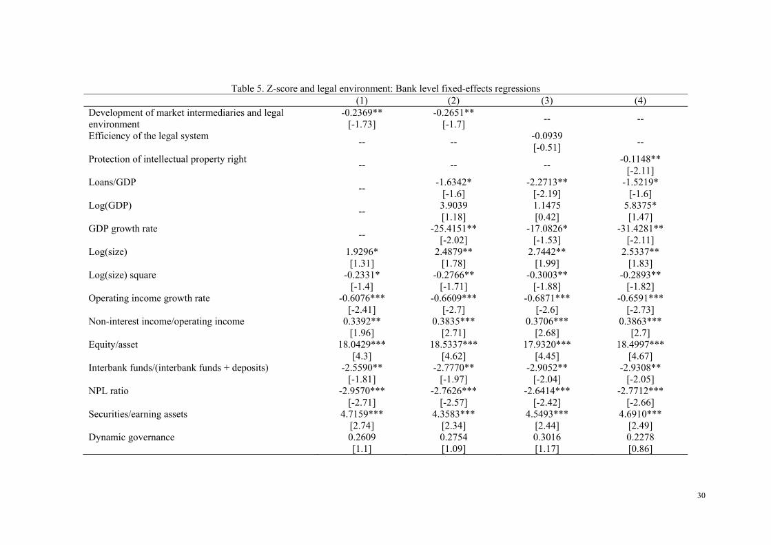
Table 5 reports the fixed effect regression results of the Z-score (log value) on the legal
environment variables and various control variables. The calculation of standard variation and
t values is clustered at the bank level. We find that measures of the legal environment are in
general negatively associated with the Z-score (again, higher value of Z-score indicates more
7In our analysis, we need to take the logarithm of both input and output factors. To avoid taking the logarithm of zero or a negative number, it is a common practice in the literature to find the minimum value for each factor (usually a negative number), calculate its absolute value plus one (∣y∣+ 1) and then add this number to the initial variable value before taking the logarithm. However, if the quantitative level of ∣y∣ is exceptionally large, then the input-output relationship may change significantly for some banks. In this paper, we adopt the following procedure to tackle this issue. We use negative one million as the benchmark and add 1.01 million to the initial value of the variable. If the result is less than 1, then we treat the logarithm value of this observation as zero. For the rest, we directly take the logarithm. Although this approach effectively imposes some “penalty” on negative values and sacrifices some information by smoothing out the variation in some variables with negative and large absolute values, it allows us better control of the potential distortion of the estimation results resulting from exceptionally large negative values. Our main results are not sensitive to the choice of the benchmark value or following the common practice to obtain the logarithm values. 8Given the difference in domestic and foreign currency transactions among banks and because RMB transactions account for the majority of the banking business in Chinese domestic financial institutions, we focus on the RMB business of banks in this paper. Foreign banks own only a small share of the total assets in the Chinese banking sector and thus are excluded from our analysis.

17
stability). This shows that better legal environment in a region encourages banks to take more
risk. Specifically, the development of market intermediaries (more lawyers and certified
accountants relative to the population) has a significantly negative coefficient (regression 2).
The coefficient on the efficiency of the regional legal system has the expected sign but the
result is insignificant (regression 3). The coefficient estimate on the protection of intellectual
property right has a negative sign as expected and is significant (at the 5% level), indicating
that better law enforcement as represented by the stronger protection of intellectual property
rights in the region increases bank risk taking (regression 3). These results are not sensitive to
the inclusion or exclusion of other macro variables in the regressions (regression 1).
[Table 5]
Examination of the coefficients on the various control variables shows interesting results
that are generally consistent with previous research (e.g. Houston et al., 2010). We find an
inverse U-shape relation between bank size and bank risk taking. In addition, banks with
higher growth rate of operating income, greater NPL ratio and higher ratio of interbank
borrowing engage in more risk taking. In contrast, banks that rely more on non-interest
income, hold more security assets, and have a greater capital ratio tend to take less risk.
4.2 Legal environment and bank efficiency: Results of the income-based model
In this section, we investigate how regional legal environment affect bank efficiency.
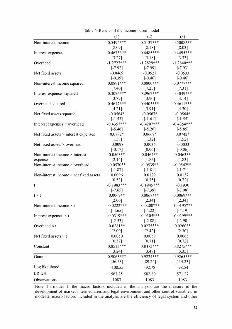
Tables 6 and 7 present the one-step maximum-likelihood estimation results using the
income-based model. All the regression models have a high γ value, indicating a high
overall significance level (at the 1% level). The signs of first-order coefficients in all the
18
regression models are as expected (Table 6) and most of the coefficient estimates are
significant (at least at the 10% level).
[Table 6]
[Table 7]
We find strong effects of regional legal environment on the efficiency of CCBs. The
comprehensive index of the development of market intermediaries and legal environment,
efficiency of the legal system, and the protection of intellectual property right are all
negatively related to the technical inefficiency of CCBs as expected (regressions 1-3 in Table
7), and the coefficients are highly significant (at the 5% level and above). In other words, a
well-developed legal environment significantly improves the efficiency level of CCBs in the
region. In addition, GDP of the region is positively correlated with the technical inefficiency
of CCBs. This finding is consistent with that of Hasan et al. (2009): when the local market is
big, more banks are attracted to the market and thus local banks (CCBs) face greater
competition, which results in a low level of efficiency among CCBs in the region. In contrast,
high growth rate of the size of the local market (as measured by GDP) will benefit all banks
in the region and result in higher bank efficiency.
The risk factors all have the expected relation with bank efficiency. We find that the
profit efficiency level among banks with a high NPL ratio is low. The equity-to-assets ratio
has a negative coefficient, indicating that a strict constraint on the capital requirement of
banks actually improves bank efficiency. Not surprisingly, the loan-to-deposit ratio has a
positive impact on bank efficiency as a greater ability to offer loans enhances bank
profitability. Similarly, the interbank fund-to-total borrowings ratio is positively related to

19
bank inefficiency, showing that banks that rely more on deposits than on short-term
borrowing are more efficient probably due to the low funding cost associated with deposits.
As for asset structure, the ratio of securities to total assets has a negative relation with bank
inefficiency, which shows that the greater allocation of bank assets to securities improves the
ability of banks to generate profit. This result can be taken as evidence that the risk-adjusted
return on securities is higher than that on other assets such as loans and cash-type assets in
China. In addition, we detect a strong effect of selection governance variable on bank
efficiency. Banks which have been selected for IPOs and foreign investment are significantly
more efficient than other.
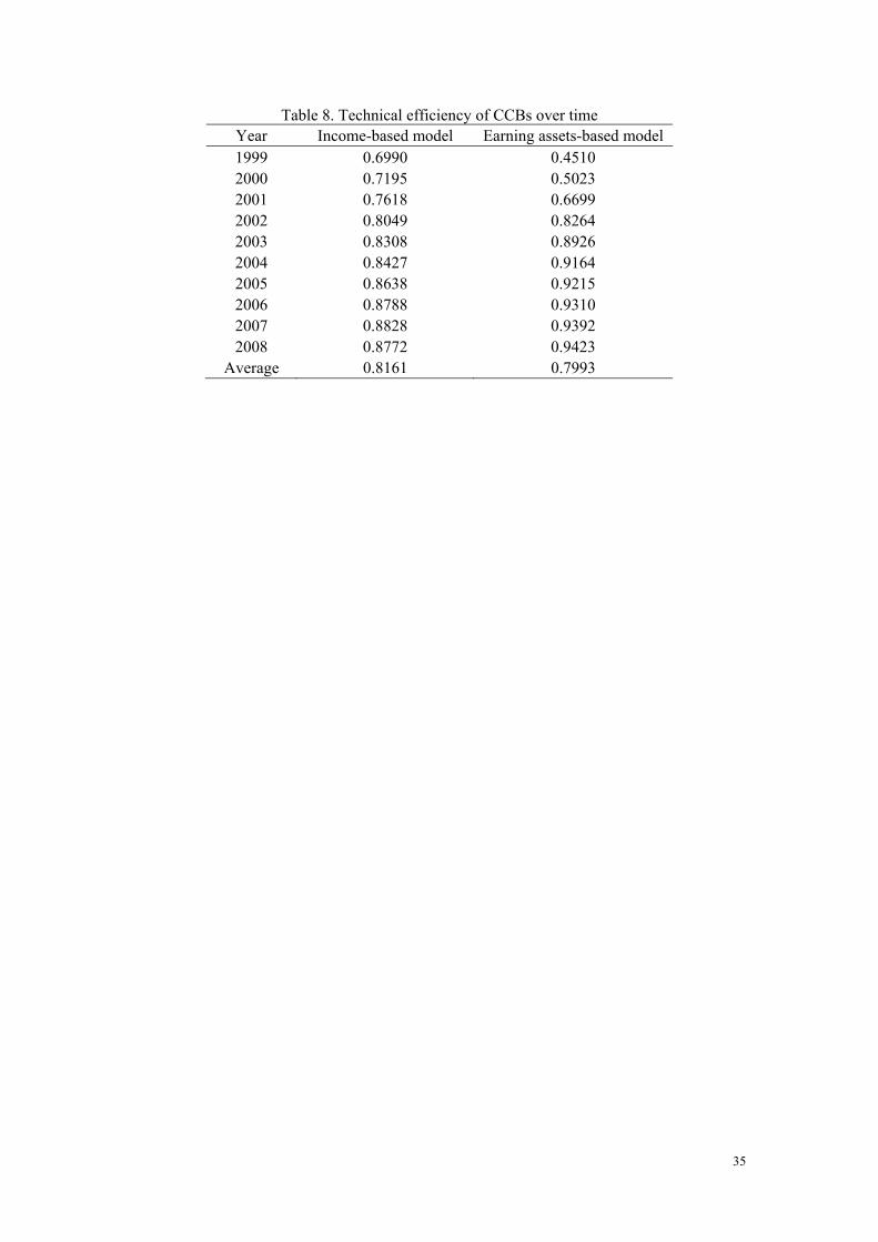
Table 8 (second column) presents the time trend of the efficiency score of CCBs using
the income-based model.9 The efficiency scores of Chinese banks show a rising trend,
especially before 2003.
[Table 8 here]
4.3 Legal environment and bank efficiency: Results of the earnings assets-based
model
An alternative model to study bank efficiency is based on the earning assets of a bank.
Table 4 lists the main differences between this model and the income-based model. Besides
the different input and output factors included, there are a few minor differences in the
variable definitions. For example, in the income-based model, net interest income is my in
equation (2), whereas in the earning assets-based model, it is measured by total deposits.
9In Tables 8, only the results of model 1 in Tables 6, 7 and 9 are reported. Efficiency scores using other models are similar and the untabulated results are available from the authors upon request.

20
Table 9 presents the maximum-likelihood estimation results using the full sample. Only
the inefficiency analysis results are reported to save space. The income-based model has a γ
value greater than that of the earning assets-based model, indicating the better model fit of the
former. Their estimation results, however, are generally similar. For example, all of the
coefficients on the legal environment variables are negative (regressions 1-3) and most of
them are significant (except the efficiency of the legal system), which indicates that a good
legal environment enhances bank efficiency. The size of the regional market also has a
negative impact on bank efficiency while its growth rate has a positive effect. The
loan-to-GDP ratio has a significantly positive coefficient in the inefficiency analysis. The
possible explanation is that in regions with a high level of financial deepening, CCBs face
more competition from the JSCBs and Big Four, which constrains the ability of the former to
expand their business. As for bank characteristics, the selection governance variable is
negatively related to technical inefficiency, a result that is similar to that of the income-based
model. Unsurprisingly, the loan to deposit ratio has a negative coefficient as a greater ability
to offer loans enhances the bank’s ability to expand business. In addition, more reliance on the
interbank borrowing reduces a bank’s efficiency.
[Table 9 here]
There are a few differences in the estimation results for bank characteristics. The
coefficient on NPL ratio is insignificant in the earning assets-based model, indicating that
NPLs have a greater effect on the profitability of banks than on the ability of banks to expand
their business. The equity-to-assets ratio has a positive sign in the earning assets-based model,
consistent with the argument that when the capital requirement is soft, banks have a greater

21
incentive to expand than to focus on capital returns (Jiang et al., 2009). As for the asset
structure of banks, the ratio of securities to total assets becomes insignificant in the earning
assets-based model. The ratio of long-term to total loans has no significant impact on the
efficiency of banks in the income-based model but is positively related to bank efficiency in
the earning assets-based model.
Table 8 (right panel) presents the efficiency scores of banks using the earning
assets-based model. The time trend of the CCBs’ efficiency using the earning assets-based
model is similar to that of the income-based model (Table 8).
5. Conclusion
We investigate bank risk taking, efficiency and their relation to legal environment using a
unique sample of 133 Chinese banks for the 1999-2008 period. We find that stronger legal
protection tends to promote greater bank risk taking in the region. Employing a stochastic
function approach, our analysis shows that the performance of Chinese banks, as measured by
bank efficiency, is heavily influenced by the legal environment in the region. More developed
market intermediaries, higher efficiency in the legal system, and better protection of
intellectual property right are associated with a higher level of efficiency among these banks.
These results are robust to alternative estimation models.

22
References
Acemoglu, D. (2005) Constitutions, politics and economics: A review essay on Persson and
Tabellini's "The Economic effects of constitutions", Journal of Economic Literature,
43, pp. 1025-1048.
Acemoglu, D., Dell, M., 2010. Productivity differences between and within countries,
American Economic Journal: Macroeconomics 2 (1), 169-188.
Allen, F., Qian, J., Qian, M., 2005. Law, finance, and economic growth in China, Journal of
Financial Economics 77 (1), 57-116.
Battese, G.E., Coelli, T.J., 1995. A model for technical inefficiency effects in a stochastic
frontier production function for panel data, Empirical Economics 120, 325-332.
Berger, A.N., Clarke, G.R.G., Cull, R., Klapper, L., Udell, G.F., 2005. Corporate governance
and bank performance: a joint analysis of the static, selection, and dynamic effects of
domestic, foreign, and state ownership, Journal of Banking and Finance 29, 2179-2221.
Berger, A.N., Hasan, I., Zhou, M., 2009. Bank ownership and efficiency in China: what will
happen in the world’s largest nation? Journal of Banking and Finance 33, 113-130.
Berger, A.N., Humphrey, D.B., 1997. Efficiency of financial institutions: international survey
and directions for future research, European Journal of Operational Research 98 (2),
175-212.
Berger, A.N., Mester, L.J., 1997. Inside the black box: what explains differences in the
efficiencies of financial institutions? Journal of Banking and Finance 21, 895-947.
Berger, A.N., Udell, G.F., 2006. A more complete conceptual framework for SME finance,
Journal of Banking and Finance 30, 2945-66.
23
Berkowitz, D., Clay, K., 2006. The effect of judicial independence on courts: evidence from
the American states, Journal of Legal Studies 35 (2), 399-400.
Chen, X., Skully, M., Brown, K., 2005. Banking efficiency in China: application of DEA to
pre- and post-deregulations era: 1993-2000, China Economic Review 16, 229-245.
Coelli, T., Perelman, S., 1996. Efficiency measurement, multi-output technologies and
distance functions: with application to European railways, CREPP Working Paper 96
(05), University of Liege.
Cole, R., Turk-Ariss, R., 2008. Legal origin, creditor protection and bank risk-taking:
evidence from emerging markets. Unpublished working paper, DePaul University,
Lebanese American University.
Demirguc-Kunt, A., Laeven, L., Levine, R., 2003. Regulations, market structure, institutions,
and the cost of financial intermediation, Journal of Money, Credit and Banking 36,
593-622.
Fan, G., Wang, X. (ed.), 2000, 2004, 2006, 2010 (in Chinese). Zhongguo shi chang hua zhi
shu: ge di qu shi chang hua xiang dui jin cheng du bao gao. Beijing: Jing ji ke xue chu
ban she.
Ferri, G., 2009. Are new tigers supplanting old mammoths in China’s banking system?
Evidence from a sample of city commercial banks, Journal of Banking and Finance 33,
131-140.
Fries, S., Taci, A., 2005. Cost efficiency of banks in transition: evidence from 289 banks in 15
post-communist countries, Journal of Banking and Finance 29, 55-81.
Fu, X., Heffernan, S.A., 2007. Cost X-efficiency in China’s banking sector, China Economic

24
Review 18, 35-53.
Hasan, I., Wang H., Zhou, M., 2009. Do better institutions improve bank efficiency? Evidence
from a transitional economy, Managerial Finance 35 (2), 107-127.
Houston, J., Lin, C., Lin, P., Ma Y., 2010. Creditor rights, information sharing, and bank risk
taking, Journal of Financial Economics 96, 485-512.
Jiang, C., Yao, S., Zhang, Z., 2009. The effects of governance changes on bank efficiency in
China: a stochastic distance function approach, China Economic Review 20, 717-731.
Laeven, L., Woodruff, C., 2007. The quality of the legal system, firm ownership, and firm
size, Review of Economics and Statistics 89 (4), 601-614.
La Porta, R., Lopez-de-Silanes, F., Shleifer, A., Vishny, R., 1998. Law and finance, Journal
of Political Economy, 106, 1113-1155.
Lovell, C.A.K., Richardson, S., Travers, P., Wood, L.L., 1994. Resources and functionings: a
new view of inequality in Australia, in W. Eichhorn (ed.), Models and Measurement of
Welfare and Inequality, Springer Verlag, Berlin, 787-807.
Ma, Y., Qu, B., Zhang, Y., 2010. Judicial quality, contract intensity and trade: firm-level
evidence from developing and transition countries, Journal of Comparative
Economics 38 (2), 146-159.
Orea, L., 2002. Parametric decomposition of a generalized Malmquist productivity index,
Journal of Productivity Analysis 18, 5-22.
Qian, J., Strahan, P.E., 2007. How laws and institutions shape financial contracts: the case of
bank loans, Journal of Finance 62, 2803-34.
Wang, H., Schmidt, P., 2002. One-step and two-step estimation of the effects of exogenous

25
variables on technical efficiency levels, Journal of Productivity Analysis 18, 129-144.
26
Table 1. Summary statistics of bank characteristics (CCBs, 1999-2008) Mean Std. Dev. Min. Max. Obs. Net interest income 323.68 644.86 -101.04 8418.23 1083 Non-interest income 15.23 52.66 -14.54 973.10 1083 Total loans 6219.47 12269.37 76.55 130384.40 1083 Deposits 10220.21 20319.47 387.73 211077.70 1083 Other earning assets 5691.75 12991.87 124.70 156363.50 1083 Interest expenses 158.89 346.65 1.90 4027.82 1083 Overhead 182.32 302.00 3.80 2907.11 1083 Net fixed assets 165.61 205.08 9.08 2064.14 1083 Equity/assets 0.0435 0.0361 -0.1273 0.3741 1083 NPL ratio 0.1588 0.1735 0.0000 0.8177 1083 Loan loss reserves/total loans 0.0139 0.0154 -0.0115 0.1147 1083 Loans/deposits 0.6143 0.1679 0.0670 1.2543 1083 Interbank funds/ (interbank funds + deposits)
0.1015 0.0947 0.0000 0.4959 1083
Long-term loans/total loans 0.3007 0.1886 0.0000 0.8431 1083 Securities/earning assets 0.1701 0.1118 0.0000 0.5185 1083
Note: Input and output factors are measured in million RMB at the 2000 price level.
27
Table 2. Sample distribution Year Number of banks 1999 84 2000 89 2001 102 2002 107 2003 108 2004 108 2005 112 2006 120 2007 120 2008 133 Total 1083
Note: In January 2007, ten CCBs (including the Wuxi Commercial Bank) merged to form the Jiangsu Commercial Bank; therefore, the number of CCBs did not greatly increase from 2006.
28
Table 3. Development of market intermediaries and legal environment Provinces 1998 1999 2000 2001 2002 2003 2004 2005 2006 2007 Beijing 9.20 4.52 5.12 7.37 7.62 7.63 8.10 7.78 7.87 8.41 Tianjin 3.97 4.05 4.35 5.86 6.50 6.95 7.49 8.51 8.98 9.92 Hebei 1.59 2.95 3.15 3.26 3.39 3.48 3.90 5.11 5.13 5.27 Shanxi 3.11 3.24 3.94 2.91 3.08 3.20 3.61 4.38 4.51 4.78 Inner Mongolia 2.30 2.87 3.42 3.30 3.38 3.56 3.96 4.47 4.43 4.50 Liaoning 3.24 3.16 3.54 4.28 4.51 5.15 5.46 6.35 6.55 7.23 Jilin 2.79 3.35 3.36 3.65 3.69 3.83 3.89 4.79 4.84 5.37 Heilongjiang 2.65 3.13 3.51 4.07 4.24 4.44 4.56 5.30 5.15 5.46 Shanghai 5.32 3.92 5.51 9.42 10.52 12.15 11.06 12.84 13.87 16.61 Jiangsu 2.17 3.66 3.76 5.20 5.69 6.18 6.61 8.18 9.07 11.50 Zhejiang 2.32 3.49 3.99 6.19 7.16 8.09 8.39 10.59 11.97 13.89 Anhui 1.34 3.15 3.05 2.53 2.67 2.63 3.15 4.99 5.53 5.99 Fujian 2.36 3.66 4.31 4.68 5.05 5.23 5.30 6.41 6.61 6.92 Jiangxi 1.55 2.76 2.59 2.23 2.61 3.01 3.38 4.32 4.28 4.75 Shandong 2.22 3.15 3.11 3.80 4.18 4.67 5.13 6.14 6.71 7.37 Henan 1.50 2.85 3.00 3.06 3.12 3.07 3.38 4.52 4.66 4.99 Hubei 2.04 2.87 3.04 2.96 3.24 3.74 3.81 4.87 5.02 5.79 Hunan 1.68 1.35 1.50 2.29 2.64 3.13 3.75 4.29 4.20 4.32 Guangdong 3.85 4.17 6.02 7.11 7.69 8.45 8.86 10.64 11.47 12.59 Guangxi 1.90 2.89 2.99 2.92 3.10 3.20 3.17 3.80 3.70 4.23 Hainan 2.09 3.73 3.93 3.86 3.80 3.64 3.57 3.63 3.74 3.87 Chongqing 2.19 2.13 1.72 2.37 2.74 3.29 3.95 4.89 5.20 5.61 Sichuan 1.96 2.65 2.43 3.49 3.81 4.03 4.11 5.04 5.24 5.96 Guizhou 1.27 2.47 2.32 1.82 1.88 1.96 2.16 3.12 3.20 3.76 Yunnan 1.85 2.26 2.74 2.17 2.33 2.41 2.75 3.91 4.15 4.63 Tibet NA NA 0.00 1.90 1.91 2.25 2.63 3.60 3.78 3.89 Shannxi 2.93 1.73 1.92 1.78 2.29 2.47 2.88 3.96 4.29 4.99 Gansu 1.45 2.27 1.89 1.15 1.36 1.52 2.11 3.34 3.57 3.79 Qinghai 1.88 2.75 3.02 1.47 1.58 1.49 1.53 1.85 2.06 2.79 Ningxia 2.37 2.92 2.58 1.67 1.86 2.24 2.83 3.47 3.52 3.80 Xinjiang 2.83 2.17 2.12 3.28 3.85 4.37 4.48 4.83 4.64 4.56 Country average 2.60 3.01 3.16 3.61 3.92 4.24 4.51 5.48 5.74 6.37

29
Table 4. Comparison of the income-based model and the earning assets-based model Income-based model Earning assets-based model
Input factors
Interest expenses, non-interest expenses (operating expenses), net value of fixed assets
Output factors
Net interest income, non-interest income
Total loans, total deposits, other earning assets, non-interest income
Note
1. Interest expenses: costs on deposits and other earning assets. 2. Non-interest expenses (operating expenses) include employee expenses,
business expenses, depreciation and amortization, business taxes and other expenses.
3. Net value of fixed assets measures the input factor of fixed assets. 4. Non-interest income includes net commission income, net exchange
income, other operating income, net income from property leasing, investment income and so forth.
5. Non-interest income is included in the earning assets-based model as an output factor to control for the impact of off-balance-sheet activities (see Orea, 2002; Fu and Heffernan, 2007; Jiang et al., 2009).
6. Deposits are regarded as both input and output, because the service provided to the depositors is closely associated with the amount of deposits.
7. Other earning assets are the remaining assets after loans and fixed assets are deducted from the total assets, including cash, deposits in the central bank and other financial institutions, reverse repurchase agreements, securities and so forth (see Orea, 2002; Fu and Heffernan, 2007; Jiang et al., 2009).
30
Table 5. Z-score and legal environment: Bank level fixed-effects regressions (1) (2) (3) (4) Development of market intermediaries and legal environment
-0.2369** [-1.73]
-0.2651** [-1.7] -- --
Efficiency of the legal system -- -- -0.0939 [-0.51] --
Protection of intellectual property right -- -- -- -0.1148** [-2.11]
Loans/GDP -- -1.6342* [-1.6]
-2.2713** [-2.19]
-1.5219* [-1.6]
Log(GDP) -- 3.9039 [1.18]
1.1475 [0.42]
5.8375* [1.47]
GDP growth rate -- -25.4151** [-2.02]
-17.0826* [-1.53]
-31.4281** [-2.11]
Log(size) 1.9296* [1.31]
2.4879** [1.78]
2.7442** [1.99]
2.5337** [1.83]
Log(size) square -0.2331* [-1.4]
-0.2766** [-1.71]
-0.3003** [-1.88]
-0.2893** [-1.82]
Operating income growth rate -0.6076*** [-2.41]
-0.6609*** [-2.7]
-0.6871*** [-2.6]
-0.6591*** [-2.73]
Non-interest income/operating income 0.3392** [1.96]
0.3835*** [2.71]
0.3706*** [2.68]
0.3863*** [2.7]
Equity/asset 18.0429*** [4.3]
18.5337*** [4.62]
17.9320*** [4.45]
18.4997*** [4.67]
Interbank funds/(interbank funds + deposits) -2.5590** [-1.81]
-2.7770** [-1.97]
-2.9052** [-2.04]
-2.9308** [-2.05]
NPL ratio -2.9570*** [-2.71]
-2.7626*** [-2.57]
-2.6414*** [-2.42]
-2.7712*** [-2.66]
Securities/earning assets 4.7159*** [2.74]
4.3583*** [2.34]
4.5493*** [2.44]
4.6910*** [2.49]
Dynamic governance 0.2609 [1.1]
0.2754 [1.09]
0.3016 [1.17]
0.2278 [0.86]

31
Constant -4.7448 [-0.66]
-54.2537 [-1.25]
-20.7348 [-0.56]
-79.4752* [-1.54]
Year yes yes yes yes Observations 559 559 559 559 Cluster 108 108 108 108 R-square (within group) 0.3462 0.3659 0.3605 0.3736
Note: The dependent variable is the natural logarithm of the Z-score. Z-score = (ROA+CAR)/σ(ROA), where ROA is the return on assets and CAR is the capital-asset ratio, both averaged over the past five years. σ(ROA) is the standard deviation of ROA over the past five years. Higher Z-score implies more stability. Operating income = interest income + non-interest income. Values of macro variables are from the previous year. t-values are computed by the robust standard errors clustered for individual banks and are presented in brackets. ***, ** and * indicate significance at the 1%, 5% and 10% levels, respectively.
32
Table 6. Results of the income-based model (1) (2) (3) Non-interest income 0.5496***
[8.09] 0.5137***
[8.18] 0.5008***
[8.03] Interest expenses 0.4673***
[3.27] 0.4485***
[3.18] 0.4495***
[3.33] Overhead -1.2727***
[-7.92] -1.2829***
[-7.99] -1.2840***
[-7.93] Net fixed assets -0.0469
[-0.39] -0.0527 [-0.46]
-0.0533 [-0.46]
Non-interest income squared 0.0891*** [7.40]
0.0800*** [7.25]
0.0777*** [7.31]
Interest expenses squared 0.3076*** [3.87]
0.2967*** [3.90]
0.3049*** [4.14]
Overhead squared 0.4617*** [4.21]
0.4405*** [3.91]
0.4611*** [4.30]
Net fixed assets squared -0.0564* [-1.53]
-0.0567* [-1.61]
-0.0564* [-1.55]
Interest expenses × overhead -0.4357*** [-5.46]
-0.4207*** [-5.26]
-0.4354*** [-5.85]
Net fixed assets × interest expenses 0.0782* [1.58]
0.0669* [1.32]
0.0742* [1.52]
Net fixed assets × overhead -0.0098 [-0.17]
0.0036 [0.06]
-0.0033 [-0.06]
Non-interest income × interest expenses
0.0563** [2.14]
0.0464** [1.85]
0.0463** [1.83]
Non-interest income × overhead -0.0570** [-1.87]
-0.0539** [-1.81]
-0.0542** [-1.71]
Non-interest income × net fixed assets 0.0096 [0.53]
0.0129 [0.75]
0.0137 [0.72]
t -0.1983*** [-7.65]
-0.1945*** [-7.39]
-0.1930 [-7.08]
t × t 0.0069** [2.06]
0.0067*** [2.34]
0.0069*** [2.34]
Non-interest income × t -0.0222*** [-4.65]
-0.0200*** [-4.22]
-0.0195*** [-4.19]
Interest expenses × t -0.0319*** [-2.53]
-0.0305*** [-2.88]
-0.0299*** [-2.90]
Overhead × t 0.0281** [2.09]
0.0275*** [2.42]
0.0260** [2.30]
Net fixed assets × t 0.0050 [0.57]
0.0059 [0.71]
0.0065 [0.72]
Constant 0.8513*** [3.24]
0.8473*** [3.48]
0.8275*** [3.35]
Gamma 0.9063*** [56.53]
0.9224*** [89.24]
0.9265*** [114.23]
Log likelihood -100.55 -92.78 -98.54 LR test 567.25 582.80 571.27 Observations 1083 1083 1083 Note: In model 1, the macro factors included in the analysis are the measure of the development of market intermediaries and legal environment and other control variables; in model 2, macro factors included in the analysis are the efficiency of legal system and other

33
control variables; in model 3, the macro factors included in the analysis are the protection of intellectual property rights and other control variables. ***, ** and * indicate significance at the 1%, 5% and 10% levels, respectively; t-values are in parentheses.

34
Table 7. Inefficiency analysis: results of the income-based model (1) (2) (3)
Development of Market Intermediaries and Legal Environment
-0.0790*** [-4.33] -- --
Efficiency of the legal system -- -0.1769*** [-8.10]
--
Protection of intellectual property right -- -- -0.0230** [-2.12]
Loans/GDP -0.1073 [-0.73]
-0.3658*** [-3.01]
-0.4781** [-2.24]
Ln (GDP) 0.4999*** [8.61]
0.6760*** [12.63]
0.4962*** [9.90]
GDP growth rate -0.0209** [-2.05]
-0.0191** [-2.00]
-0.0355* [-1.35]
Selection governance -1.5023*** [-7.42]
-1.1770*** [-5.76]
-1.3868*** [-6.80]
Dynamic governance 0.2535 [0.74]
0.4978*** [3.98]
0.5011*** [2.62]
Equity/assets -7.0936*** [-8.32]
-8.0675*** [-10.53]
-8.2276*** [-8.93]
NPL ratio 4.6967*** [9.90]
5.1799*** [11.57]
5.4355*** [12.82]
Loan loss reserves/loans -2.1652** [-2.06]
-0.3348 [-0.31]
0.5101 [0.41]
Loans/deposits -2.8358*** [-9.61]
-3.0953*** [-11.94]
-3.3164*** [-10.26]
Interbank funds/(interbank funds + deposits)
1.2132*** [4.96]
1.0359*** [3.76]
1.1492*** [3.93]
Long-term loans/loans 0.1637 [1.25]
-0.1726 [-1.10]
-0.0878 [-0.51]
Securities/earning assets -3.5277*** [-9.30]
-4.3132*** [-11.71]
-4.0642*** [-9.18]
Constant -3.9565*** [-3.88]
-5.8261*** [-5.09]
-2.2807 [-0.83]
Note: see Table 6.
35
Table 8. Technical efficiency of CCBs over time Year Income-based model Earning assets-based model 1999 0.6990 0.4510 2000 0.7195 0.5023 2001 0.7618 0.6699 2002 0.8049 0.8264 2003 0.8308 0.8926 2004 0.8427 0.9164 2005 0.8638 0.9215 2006 0.8788 0.9310 2007 0.8828 0.9392 2008 0.8772 0.9423
Average 0.8161 0.7993

36
Table 9. Inefficiency analysis: results of the earning assets-based model (1) (2) (3) Development of Market Intermediaries and Legal Environment
-0.0469*** [-4.87]
-- --
Efficiency of the legal system -- -0.0068 [-1.17]
--
Protection of intellectual property right -- -- -0.0166*** [-4.04]
Loans/GDP 0.1280** [2.18]
0.0266 [0.47]
0.1398*** [2.61]
Ln (GDP) 0.1274*** [5.82]
0.0716*** [3.29]
0.1088*** [5.22]
GDP growth rate -0.8313 [-0.97]
-2.4417** [-2.02]
-1.1726* [-1.46]
Selection governance -0.0933*** [-2.57]
-0.0558* [-1.59]
-0.0767** [-2.23]
Dynamic governance 0.0637 [0.90]
0.0689 [1.07]
0.0418 [0.74]
Equity/assets 0.3481* [1.29]
0.2915 [1.02]
0.3066 [1.15]
NPL ratio 0.0266 [0.37]
0.0156 [0.21]
0.0419 [0.59]
Loan loss reserves/loans 0.9348* [1.57]
0.8652* [1.47]
0.6869 [1.17]
Loans/deposits -1.2231*** [-5.37]
-1.2149*** [-5.49]
-1.3681*** [-7.52]
Interbank funds/(interbank funds + deposits)
0.3916*** [2.96]
0.5151*** [4.05]
0.4673*** [3.85]
Long-term loans/loans -0.2940*** [-4.99]
-0.2776*** [-4.51]
-0.2445*** [-3.92]
Securities/earning assets -0.1039 [-1.13]
-0.1258 [-1.19]
-0.1032 [-1.12]
Constant -0.2140 [-0.65]
0.5393** [1.81]
0.0308 [0.10]
Gamma 0.3180*** [4.10]
0.2709*** [3.08]
0.2831*** [3.39]
Log likelihood 395.67 383.60 392.87 LR test 147.53 123.40 141.94 Observations 1083 1083 1083
Note: ***, ** and * indicate significance at the 1%, 5% and 10% levels, respectively; t-values are in parentheses.