Bank of England Staff Working Paper No. 612

C CO CO C CO COD

C CO C CO CO CO C CO COD





























Staff Working Paper No. 612Finance and SynchronizationAmbrogio Cesa-Bianchi, Jean Imbs and Jumana Saleheen

August 2016

Staff Working Papers describe research in progress by the author(s) and are published to elicit comments and to further debate. Any views expressed are solely those of the author(s) and so cannot be taken to represent those of the Bank of England or to stateBank of England policy. This paper should therefore not be reported as representing the views of the Bank of England or members ofthe Monetary Policy Committee, Financial Policy Committee or Prudential Regulation Authority Board.

Staff Working Paper No. 612Finance and SynchronizationAmbrogio Cesa-Bianchi,(1) Jean Imbs(2) and Jumana Saleheen(3)

Abstract

In the workhorse model of international real business cycles, financial integration exacerbates the cycle asymmetry created by country-specific supply shocks. The prediction is identical in response topurely common shocks in the same model augmented with simple country heterogeneity (eg, wheredepreciation rates or factor shares are different across countries). This happens because common shockshave heterogeneous consequences on the marginal products of capital across countries, which triggersinternational investment. In the data, filtering out common shocks requires therefore allowing forcountry-specific loadings. We show that finance and synchronization correlate negatively in response tosuch common shocks, consistent with previous findings. But finance and synchronization correlate non-negatively, almost always positively, in response to purely country-specific shocks.

Key words: Financial linkages, business cycles synchronization, contagion, common shocks,idiosyncratic shocks.

JEL classification: E32, F15, F36, G21, G28.

(1) Bank of England and CfM. Email: [email protected](2) Paris School of Economics (CNRS) and CEPR. Email: [email protected](3) Bank of England. Email: [email protected]

We would like to thank Michael Binder, Giancarlo Corsetti, Richard Harrison, Sujit Kapadia, Robert Kollmann, Eric Monnet,Jose-Luis Peydro, Franck Portier, Daniele Siena, Konstantinos Theodoridis and Gregory Thwaites for helpful comments andsuggestions. We are also grateful for comments from attendants to the 10th Annual Workshop on ‘The Macroeconomics ofGlobal Interdependence’ in Dublin, the IAAE 2016 Annual Meetings, the ‘Workshop on International Business Cycles’ atBanque de France, and seminar participants at the ECB and the Bank of England. Financial support from the Chaire Banque de France at the Paris School of Economics is gratefully acknowledged. The views expressed in this paper are solely those ofthe authors and should not be taken to represent those of the Bank of England.

Information on the Bank’s working paper series can be found atwww.bankofengland.co.uk/research/Pages/workingpapers/default.aspx

Publications Team, Bank of England, Threadneedle Street, London, EC2R 8AH Telephone +44 (0)20 7601 4030 Fax +44 (0)20 7601 3298 email [email protected]

© Bank of England 2016ISSN 1749-9135 (on-line)

1 Introduction

Understanding how disturbances propagate across countries is of first-order impor-

tance. Openness in general is often singled out as a plausible and significant propa-

gation channel. Historically openness to goods trade came first, and there is robust

evidence that trade partners display correlated business cycles.1 The global con-

sequences of the 2007-2008 recession have contributed to shifting the focus on the

importance of financial linkages. While it was always important to assess how fi-

nancial integration affects the international synchronization of business cycles, the

question has become of paramount importance since 2008, for policy-makers and

researchers alike.

In the canonical two-country real business cycles model with country-specific

productivity shocks (Backus, Kehoe, and Kydland, 1992, BKK henceforth) capital

flows to wherever returns are higher. Therefore, greater financial linkages lower

the international synchronization of business cycles in response to country-specific

shocks. But in a similar two-country model, augmented with credit or collateral

constraints, a country-specific shock that makes the constraint binding at home is

contagious abroad as domestic agents recall foreign assets to meet the constraint.2

There is no reason for the constraint to become binding in response to a specific

kind of shock: demand, supply, or even financial shocks may all create a binding

constraint, and so trigger contagion. Here, therefore, greater financial linkages can

increase synchronization in response to country-specific shocks. The common fea-

ture of these models is that they analyze the consequences of purely idiosyncratic,

country-specific shocks, with ambiguous predictions.

It is not difficult to see that similar predictions arise from the canonical interna-

tional RBC model in response to common shocks, provided that some mild hetero-

geneity exists across countries. For instance, countries with different depreciation

rates or different capital shares react to the same technology shock with different

magnitudes, driving a gap between the marginal products of capital on impact. As a

result, international investment rises, and the international synchronization of cycles

falls. In fact, the predictions of BKK with homogeneous countries and idiosyncratic

1Among many others, see Frankel and Rose (1998) or Baxter and Kouparitsas (2005).2See Devereux and Yetman (2010), Dedola and Lombardo (2012), Kalemli-Ozcan, Papaioan-

nou, and Perri (2013), or Allen and Gale (2000) offer different versions of the mechanism, whereconstraints are at bank or firm level.

1

Staff Working Paper No. 612 August 2016

shocks are observationally equivalent to its predictions with heterogeneous countries

and common shocks, for plausible parametrization of heterogeneity.

Figure 1 Impulse Response Functions in Variants of BKK

5 10 15 20

-0.2

0

0.2

0.4

0.6

0.8

1

1.2

1.4

(A) Idiosyncratic shock to Home

productivity (identical economies)

5 10 15 20

0

0.2

0.4

0.6

0.8

1

(B) Common shock to Home and Foreign

productivity (heterogeneous economies)

Home

Foreign

Note. Panel (A) reports the impulse response functions to a producivity shock in theHome country, in the case where the Home and Foreign economies are identical. Thechart reports the response of Output in the Home (solid line) and Foreign (dashed line)economies. Panel (B) reports the same impulse response functions for a common shock(i.e., a shock that raises productivity by the same amount in the Home and Foreigneconomy) when the two economies are heterogeneous. The source of heterogeneity is theshare of capital in the production function (θ). While in Panel (A), as in BKK, we setθH = θF = 0.36, in Panel (B) we set θH = 0.44 and θF = 0.32. All remaining parametersare identical to BKK (except for the time to build, set to 1). The size of the shock hasbeen normalized so that it increases Home output by 1 percent.

Figure 1 plots the responses of output to a technology shock as implied by two

versions of BKK. Panel (A) reproduces the well known results in BKK in response

to a shock to productivity in the Home country, under the conventional symmetric

calibration. Panel (B) introduces a version of BKK that deviates from the original in

two dimensions: (i) the productivity shock is common, i.e. is perfectly synchronized

across countries; and (ii) the share of capital is heterogeneous across countries,

taking values of 0.44 in the Home country, and 0.32 in the Foreign country (a

dispersion consistent with the values for Portugal and Japan reported in the Penn

World Tables, version 8.1, see Appendix A1). On impact, the responses of Output

in Figure 1 are virtually indistinguishable across Panels.

To investigate the ambiguous link between finance and synchronization in re-

2


sponse to country-specific shocks, it is therefore important to control for common

shocks that are allowed to have different effects across countries. The conventional

approach consists in including time effects or trends in an estimation where the

dependent variable is a measure of synchronization. This does eliminate the ef-

fects of those shocks that by construction have identical effects on both economies.

But it does not eliminate common shocks with heterogeneous effects, that are likely

to exist in a world where countries display fundamental differences, if only in the

parametrization of their production function.

To eliminate common shocks with heterogeneous effects, alternative approaches

are necessary. This paper follows the simplest possible approach: we perform a

principal component analysis on the panel of GDP growth rates, which allows us

to separate common shocks with heterogeneous effects (i.e., the country-specific

loadings on the principal components) and idiosyncratic shocks. In the main text,

the loadings are assumed constant, but for robustness we also repeat the analysis

estimating a factor model that allows for time-varying loadings using Bayesian tech-

niques. Both decompositions have the advantage of simplicity and an established

place in the literature. There are of course many alternatives, which we leave for

further work. However, we also provide analytically a general intuition for the re-

sults of the paper, that is not conditioned on one specific way to isolate common

shocks with heterogeneous effects.

Conditional on common shocks, we find that finance and synchronization cor-

relate negatively. The result supports Kalemli-Ozcan, Papaioannou, and Peydro

(2013) (KPP henceforth), who show that an increase in financial integration causes

a fall in business cycle synchronization in 18 OECD countries. But our interpreta-

tion differs from theirs. According to KPP, the data support the view that financial

flows are efficient in their quest for high returns, behaving exactly as the canonical

international RBC model predicts in response to idiosyncratic shocks. We conclude

instead that the finding arises in response to common shocks with heterogeneous

effects. Now these effects are given parametrically: they represent the response of

country i to a common shock, which differs from the response of country j be-

cause, say, the countries have different capital shares. The difference in responses

is therefore a constant, given by the differences in deep parameters of the model.

Empirically, the response of a given country to the common shock is given by the

loading in the principal component estimation: we call it the country’s “elasticity of

3


GDP”.3 Our results show that, in the cross-section, these elasticities are systemat-

ically related to capital flows. An interpretation of this finding is that capital flows

are procyclical: that is, countries with elastic GDP are net recipients of international

capital in years of global boom, but net contributors in years of global recession.4

We document this correlation in OECD data. In years of positive common shocks,

net capital holdings increase in countries with elastic GDP, and fall in countries with

inelastic GDP. The opposite tends to occur in years of negative common shocks.

In contrast, there is no systematic time pattern in the response of interna-

tional investment to purely country-specific shocks: source and destination countries

change randomly over time, depending on the realization of the shocks. Interestingly,

increases in financial linkages are almost always associated with more synchronized

business cycles in response to country-specific shocks. The coefficient estimates are

never negative, and significantly positive in 10 out of the 12 specifications we con-

sider.5 This stands in contrast with common shocks, and suggests financial links may

in fact foster the contagious propagation of country-specific shocks across borders.

In theory, the result supports the existence of (endogenously binding) constraints: in

response to country-specific shocks, financial flows may serve to alleviate collateral

or balance sheet constraints, rather than to take advantage of attractive differentials

between returns across countries.

Can we easily interpret common and idiosyncratic shocks in terms of changes

in technology, in demand, or in financial health? This is an important question in

light of the Great Recession of 2008, often understood as a financial shock that was

fundamentally different from the preceding history. For instance, Kalemli-Ozcan,

Papaioannou, and Perri (2013) construct a simple model that implies financial con-

tagion via financial shocks, and show empirically that finance and synchronization

moved in the same direction during the Great Recession. They interpret the shock

in 2008 as fundamentally different from the preceding history during which finance

and synchronization went in opposite directions. We emphasize that our decompo-

sition is just a generalization of the conventional empirical approach that controls

3Even when we allow for it, we find little time variation in the estimated factor loadings. Seethe robustness exercise in section 4.

4(See, among others, Kaminsky, Reinhart, and Vegh, 2005, Rey, 2013, Broner, Didier, Erce, andSchmukler, 2013, Bruno and Shin, 2015).

5The two non-positive estimates arise when synchronization is measured by Pearson correlationcoefficients, which are known to be problematic when the variance of the underlying shocks isvarying over time. See Forbes and Rigobon (2002).

4


for common shocks using year effects: our common shocks are more general, and of

course they nest the special case of common shocks with similar effects across coun-

tries. What we identify as “idiosyncratic shocks” is merely a subset of the shocks

considered, among others, in Kalemli-Ozcan, Papaioannou, and Perri (2013), one

that controls for common shocks with heterogeneous effects. There is neither more

nor less reason to call these shocks “demand”, “supply” or “financial” in this paper

than there are elsewhere in this literature. We argue it is only idiosyncratic shocks

that have ambiguous consequences on the link between finance and synchronization,

not common ones. The claim is true irrespective whether these shocks are to the

supply, the demand, or the financial side of the economy.

Recent Literature. Unsurprisingly, the recent years have witnessed a plethora of

models where financial integration results in contagion. Early contributions include

Devereux and Yetman (2010) where contagion is triggered by leverage-constrained

investors, whose constraint becomes binding in response to a country-specific shock

(to supply, demand, or otherwise). As portfolios are modified accordingly, the lever-

age constraint becomes binding elsewhere, with contagious consequences. Devereux

and Yu (2014) extend the model to investigate the welfare consequences of financial

integration. Dedola and Lombardo (2012) emphasize the importance of globally cor-

related borrowing costs in creating contagious finance between leveraged investors.

The common feature of these theories is the presence of financial frictions, which

result in contagious country-specific shocks (to supply, demand, or otherwise) pro-

vided that they result in endogenously binding constraints.

The empirical literature is equally replete with analyses of whether financial

linkages are contagious or not. In an early contribution, Morgan, Rime, and Strahan

(2004) investigate how bank ownership across US states affect fluctuations in Gross

State Products. They find the lifting of branching regulations between 1976 and 1994

resulted in synchronized states’ business cycles. Imbs (2006) finds a similar result

in a cross-section of countries, using alternative measures of international financial

integration. Kalemli-Ozcan, Papaioannou, and Peydro (2013) argue the finding is

driven by permanent features of country pairs, which result in both synchronized

cycles and financial linkages. In 18 OECD countries, they show the link between

finance and synchronization becomes negative once country-pair specific intercepts

are accounted for. The results are confirmed by Duval, Li, Saraf, and Seneviratne

(2016) in 63 advanced and emerging countries between 1995 and 2013. Monnet and

5


Puy (2016) show that the share of the variance of GDP explained by global shocks

is lowest during periods of financial integration, which suggests idiosyncratic shocks

are more prevalent in those periods.

It is well known that the bulk of the volatility in GDP across countries can be

explained by common shocks. In a series of influential papers, Kose, Otrok, and

Whiteman (2003, 2008), Crucini, Kose, and Otrok (2011), or Hirata, Kose, and

Otrok (2013) identify the contribution of common shocks (global or regional) to

individual countries’ business cycles. A key result is that shocks common to two or

more countries constitute the main driver of business cycles in both the developed

and developing worlds. The details of the decompositions depend on the sample

of countries and time coverage; but common shocks rarely explain less than half of

GDP growth volatility, and often more than 75 percent.

The possibility that common shocks have heterogeneous loadings is an old tra-

dition in empirical macroeconomics. Forni and Reichlin (1998) identify sector-level

effects of aggregate shocks in the US. Bernanke, Boivin, and Eliasz (2005) aug-

ment standard Vector Auto-Regressions with unobserved factors to identify their

potentially heterogeneous consequences on economic activity. Mumtaz, Simonelli,

and Surico (2011) extend the approach to an international context. Peersman and

Smets (2005) identify heterogeneous effects of monetary shocks at sector level. Kil-

ian (2008) shows the consequences of exogenous oil shocks are heterogeneous across

G7 countries.

The rest of the paper is structured as followed. Section 2 presents the conven-

tional estimation of the effects of finance on synchronization. Common shocks are

discussed in terms of their theoretical impact on the correlation between finance and

synchronization. Section 3 introduces the data that we use in the empirical analy-

sis, and discusses the relevance of common vs. idiosyncratic shocks in GDP data.

The decomposition is then used to discuss the effects of finance on synchronization.

Section 4 discusses some extensions. Section 5 concludes.

6


2 Finance and Synchronization: Why Common Shocks

Matter

This section first discusses the consequences of common shocks on business cycle

synchronization, and then turns to the consequences of common shocks on the esti-

mated effect of finance on synchronization.

2.1 Synchronization

It has become standard to measure the synchronization between two economies i

and j on the basis of the absolute differential in GDP growth Sij,t given by:

Sij,t = − |yi,t − yj,t| , (1)

where yi,t and yj,t are the growth rates of GDP in country i and j at time t. The def-

inition is such that Sij,t increases with the degree of synchronization, with negative

values close to zero between synchronized countries.

The variable Sij,t presents two key advantages. First, it is readily observable

at high frequencies, yearly or quarterly. Second, unlike the Pearson correlation

coefficient, it is invariant to the volatility of the underlying shock (see Forbes and

Rigobon (2002) and Corsetti, Pericoli, and Sbracia (2005)). However, its properties

are ambivalent. Even if two countries respond in the same direction to a shock,

i.e. co-movement is high, Sij,t can fall if the magnitude of the responses is different

across countries. In other words, Sij,t conflates a measure of co-movement and a

measure of dispersion. The same is of course not true of the more conventional

Pearson correlation coefficient.6

The measure in equation (1) is now used widely, for example by Giannone, Lenza,

and Reichlin (2010), Kalemli-Ozcan, Papaioannou, and Perri (2013), Kalemli-Ozcan,

Papaioannou, and Peydro (2013), or IMF (2013) among others. Morgan, Rime, and

Strahan (2004), Kalemli-Ozcan, Papaioannou, and Perri (2013), or Kalemli-Ozcan,

Papaioannou, and Peydro (2013) introduce an alternative that controls for common

shocks, given by:

Seij,t = − |ei,t − ej,t| , (2)

6Nor is it of the quasi-correlation coefficient in Duval, Li, Saraf, and Seneviratne (2016).

7


where ei,t is a residual of a panel growth regression:

yi,t = αi + γt + ei,t. (3)

As is clear, Seij,t controls for shocks that are common across the panel of GDP growth

rates, but that are constrained to have homogeneous effects across countries.

This paper argues the existence of common shocks with country-specific effects

alters the interpretation of Sij,t (or Seij,t). To see this, assume the true model for

GDP growth involves a vector of common shocks Fyt with heterogeneous country

loadings, i.e.:

yi,t = ayi + byiFyt + εyi,t. (4)

where ayi is the average growth of GDP in country i, εyi,t denotes the response of

GDP growth to an idiosyncratic shock, and byi is the vector of country i’s loading

on a f × 1 vector of common (to at least two countries) factors Fyt .7 By definition,

the synchronization measure in equation (1) can be re-written as:

Sij,t = −∣∣∣ayi − ayj +

(byi − b

yj

)Fyt + εyi,t − ε

yj,t

∣∣∣ . (5)

The equilibrium response of synchronization to idiosyncratic shocks is given by:

Sεij,t = −∣∣∣εyi,t − εyj,t∣∣∣ , (6)

which differs from Sij,t because of the equilibrium response of GDP in both countries

to the common shocks summarized in Fyt . Denote the guilty term by:

SFij,t = −∣∣∣(byi − byj)Fyt ∣∣∣ . (7)

By definition, SFij,t varies with both dimensions of the panel, and so has the potential

to affect the behaviour of Sij,t meaningfully, even in a regression controlling for

country-pair fixed and for year effects. Inasmuch as it only controls for common

shocks with a single loading, Seij,t suffers from the same potential issue.

Figure 2 reports the behaviour of the synchronization measure Sij,t (solid line)

in the cross-section of 18 advanced economies from 1980 to 2012, together with its

7This is a very standard assumption in the factor models literature. See Forni and Reichlin(1998) or Bernanke, Boivin, and Eliasz (2005).

8


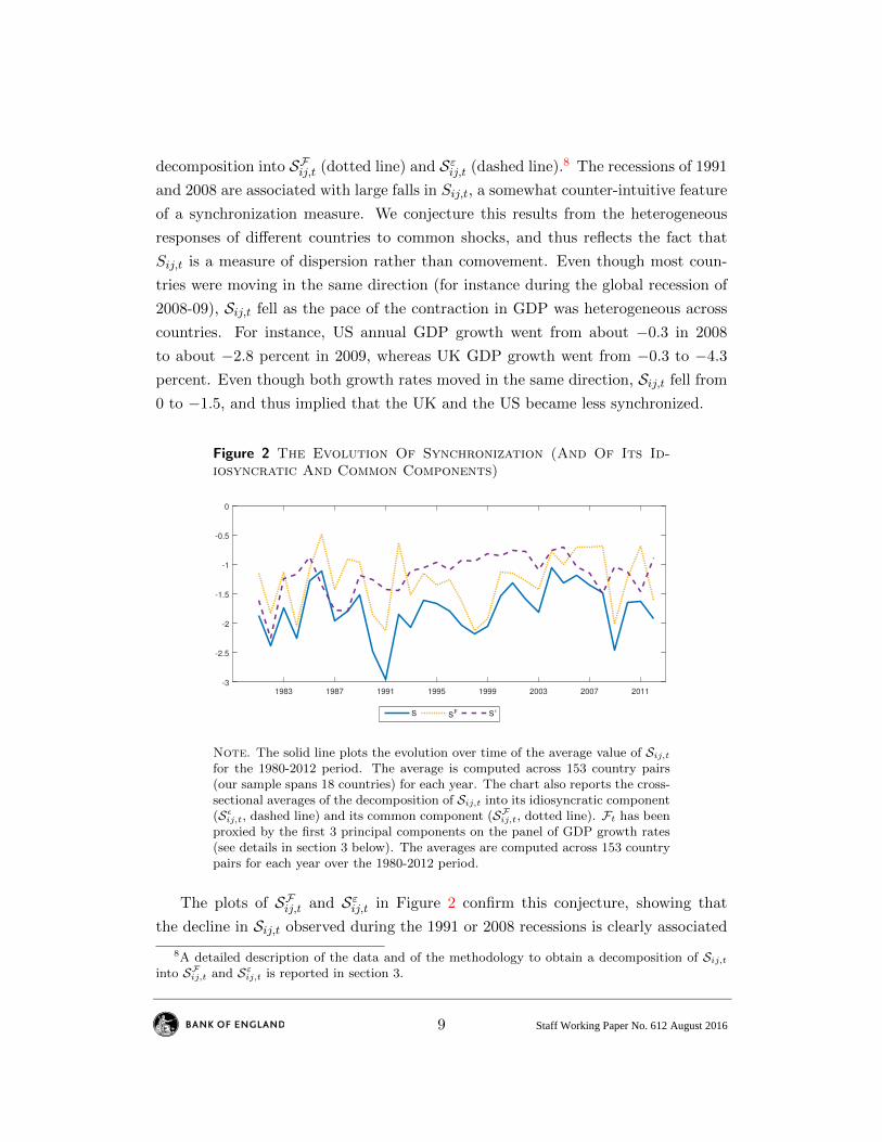
decomposition into SFij,t (dotted line) and Sεij,t (dashed line).8 The recessions of 1991

and 2008 are associated with large falls in Sij,t, a somewhat counter-intuitive feature

of a synchronization measure. We conjecture this results from the heterogeneous

responses of different countries to common shocks, and thus reflects the fact that

Sij,t is a measure of dispersion rather than comovement. Even though most coun-

tries were moving in the same direction (for instance during the global recession of

2008-09), Sij,t fell as the pace of the contraction in GDP was heterogeneous across

countries. For instance, US annual GDP growth went from about −0.3 in 2008

to about −2.8 percent in 2009, whereas UK GDP growth went from −0.3 to −4.3

percent. Even though both growth rates moved in the same direction, Sij,t fell from

0 to −1.5, and thus implied that the UK and the US became less synchronized.

Figure 2 The Evolution Of Synchronization (And Of Its Id-iosyncratic And Common Components)

1983 1987 1991 1995 1999 2003 2007 2011-3

-2.5

-2

-1.5

-1

-0.5

0

S SF S

ǫ

Note. The solid line plots the evolution over time of the average value of Sij,tfor the 1980-2012 period. The average is computed across 153 country pairs(our sample spans 18 countries) for each year. The chart also reports the cross-sectional averages of the decomposition of Sij,t into its idiosyncratic component(Sεij,t, dashed line) and its common component (SFij,t, dotted line). Ft has beenproxied by the first 3 principal components on the panel of GDP growth rates(see details in section 3 below). The averages are computed across 153 countrypairs for each year over the 1980-2012 period.

The plots of SFij,t and Sεij,t in Figure 2 confirm this conjecture, showing that

the decline in Sij,t observed during the 1991 or 2008 recessions is clearly associated

8A detailed description of the data and of the methodology to obtain a decomposition of Sij,tinto SFij,t and Sεij,t is reported in section 3.

9


with common shocks and their heterogeneous impact, as SFij,t drops substantially

in both cases. We emphasize this does not have to be the case: Sij,t does not

have to systematically take low values during recessions. The facts that it does in

OECD data, and that Sij,t is highly positively correlated with SFij,t both suggest that

common shocks with heterogeneous effects are relevant in the sample at hand. In

contrast, Sεij,t increases in 2008, and does not fall in 1991. In fact, Sεij,t reflects what

is expected of an average of idiosyncratic shocks: low volatility over the period, with

average values much closer to zero than Sij,t or SFij,t, and no systematic association

with a specific episode or a specific kind of shock (financial, oil, or monetary).

This suggests that the measure Sij,t conflates two mechanisms: the international

propagation of idiosyncratic shocks, Sεij,t, and the international equilibrium response

to common shocks, SFij,t. The former is a measure of synchronization in response

to country-specific shocks; the latter is a measure of the dispersion in GDP growth

rates in response to common shocks. This distinction complicates the estimated

effect of financial integration on synchronization.

2.2 The Effects of Finance on Synchronization

The conventional panel regression that investigates the impact of financial integra-

tion on synchronization is due to KPP. It writes:

Sij,t = αij + γt + β ·Kij,t + δ · Zij,t + ηij,t, (8)

where Kij,t measures bilateral financial linkages between i and j, and Zij,t denotes

a vector of controls, for instance bilateral goods trade. The year effects γt account

for global shocks that affect all countries homogeneously. The country-pair specific

effect αij ensures β is estimated over time, in deviations from country-pair averages,

which constitutes a substantial improvement relative to earlier estimations typically

obtained in cross-section. See for instance Frankel and Rose (1998), Doyle and Faust

(2005), Imbs (2006) or Baxter and Kouparitsas (2005), among many others. While

estimates of β are positive and significant in cross-section regressions, KPP show

they switch signs and become significantly negative within country-pairs. Since the

theory that underpins equation (8) models the propagation of shocks over time,

the estimation should include country-pair fixed effects. The resulting negative

10


estimates of β are suggestive that financial integration exacerbates the asymmetry

caused by country-specific shocks. This is the interpretation espoused by KPP.

This paper argues the existence of common shocks in equation (8) can affect the

estimates of β. The previous section argues common shocks are mechanically em-

bedded in Sij,t, provided they have heterogeneous country-specific effects. Consider

now the possibility that common shocks also affect bilateral capital linkages. This

is a well charted area. For instance Forbes and Warnock (2012) document that a

key driving force of gross capital flows are changes in global risk. Rey (2013) argues

capital flows worldwide obey global factors. Bruno and Shin (2014) document that

changes in the VIX affect the cyclicality in capital flows worldwide. For simplicity,

we posit a straightforward relation between capital cross-holdings and (common or

idiosyncratic) shocks, i.e.:

Kij,t = aKij + bKijFKt + εKij,t. (9)

This specification allows for permanent differences in capital cross-holdings, aKij , for

idiosyncratic shocks to bilateral capital εKij,t, and for a vector of common shocks

FKt . Common shocks can have heterogeneous consequences across country pairs,

captured by bKij . The specification is general, in that it can account for global

cycles in financial integration, or for a potential trend in Kij,t. If financial flows are

procyclical (as in Kaminsky, Reinhart, and Vegh, 2005, Rey, 2013, Broner, Didier,

Erce, and Schmukler, 2013, Bruno and Shin, 2015, for example), we should have

bKij ≥ 0. If Kij,t displays an upward trend, FKt takes positive and rising values in t.

In order to bring into focus the role of common shocks, consider a version of

equation (8) where the dependent variable is SFij,t. The equation becomes:

− |byi − byj | · |F

yt | = αij + γt + βF ·

[aKij + bKijFKt + εKij,t

]+ δ · Zij,t + ηFij,t. (10)

where we used the fact that:

SFij,t = −∣∣∣(byi − byj)Fyt ∣∣∣ = −

∣∣∣byi − byj ∣∣∣ · |Fyt | . (11)

Clearly, the sign of βF is given by:

Cov[−∣∣∣byi − byj ∣∣∣ · |Fyt | , bKijFKt ] = −

∣∣∣byi − byj ∣∣∣ · bKij Cov [|Fyt | ,FKt ] . (12)

11


where Cov[·] denotes the covariance operator. According to equation (12), a negative

estimate of βF requires, for example, a positive covariance between |byi − byj | and bKij

and a positive covariance between |Fyt | and FKt .

In what follows, we show that |byi − byj | and bKij display a positive correlation in

OECD data, i.e. GDP growth and capital flows happen to be responsive to common

shocks in the same countries. One possible interpretation is that this finding arise

because of the procyclicality of capital flows: countries with elastic GDP are the

systematic destination of capital flows during global (or regional) booms, but their

source in global (or regional) recessions. We show that this pattern holds in our

data. We also show that |Fyt | and FKt correlate positively, which in turn implies

that Fyt and FKt do not correlate perfectly.9 In our data, Cov[|Fyt |,FKt ] ranges from

0.20 to 0.50.

We emphasize these results are driven by permanent features of GDP growth

and of capital flows, that prevail systematically in response to common shocks.

They reflect the fact that permanent differences exist across countries in terms of

how GDP growth and capital flows respond to common shocks. But they are silent

on the response of financial flows to country-specific developments, and its conse-

quence on synchronization. The issues just discussed are absent when the measure

of synchronization is conditioned on idiosyncratic shocks. By definition, idiosyn-

cratic shocks do not display any permanent cross-sectional pattern, and therefore

Sεij,t = −∣∣∣εyi,t − εyj,t∣∣∣ cannot correlate systematically with bKij .

3 Results

This section first introduces the various data sources that have now become standard

in this literature. It then moves to a description of the paper’s key results.

3.1 Data

Annual data on GDP at constant prices are collected from the OECD National

Accounts. GDP is measured using the expenditure approach, and deflated with

each country’s GDP deflator. Bilateral financial linkages are obtained from the

9If Fyt and FKt were perfectly correlated, then cov[|Fyt |,FKt ] would be zero.

12


“International Locational Banking Statistics” released by the Bank for International

Settlements (BIS). The data collect information on international financial claims

and liabilities of banks resident in a BIS reporting country, vis-a-vis counterparty

countries. The data are in USD, and deflated using the US GDP deflator. They focus

on bank linkages, and are therefore of somewhat limited scope. But few alternatives

exist that measure bilateral financial linkages over time for other classes of assets.

The only option are the surveys collected by the International Monetary Fund as

part of the Coordinated Portfolio Investment Survey, which collect information on

all classes of financial assets. But the time coverage is limited to the 2000’s, and is

very sparse for the early years.

Data coverage is best for reporting countries, which include most developed

economies. It is much more incomplete for counterparty countries that include

many developing economies, where a lot of data points are missing. The practice

has been to combine information about claims and liabilities in both directions. For

instance, information on liabilities due by counterparty country j towards country

i is completed by data on claims held by reporting country i in country j. In

addition, given the recent globalization in financial flows, the data are normalized,

by population or GDP. In particular, consider two measures for Kij,t:

Kpopij,t =

1

4

[ln

(Aij,t

Pi,t + Pj,t

)+ ln

(Lij,t

Pi,t + Pj,t

)+ ln

(Aji,t

Pi,t + Pj,t

)+ ln

(Lji,t

Pi,t + Pj,t

)],

(13)

and:

Kgdpij,t =

1

4

[ln

(Aij,t

Yi,t + Yj,t

)+ ln

(Lij,t

Yi,t + Yj,t

)+ ln

(Aji,t

Yi,t + Yj,t

)+ ln

(Lji,t

Yi,t + Yj,t

)],

(14)

where Aij,t (Lij,t) denotes the claims (liabilities) on country j held by banks located

in country i, Yi,t is GDP in country i and time t, and Pi,t is population in country i

at time t. Both measures are bilateral; they contain no information on the direction

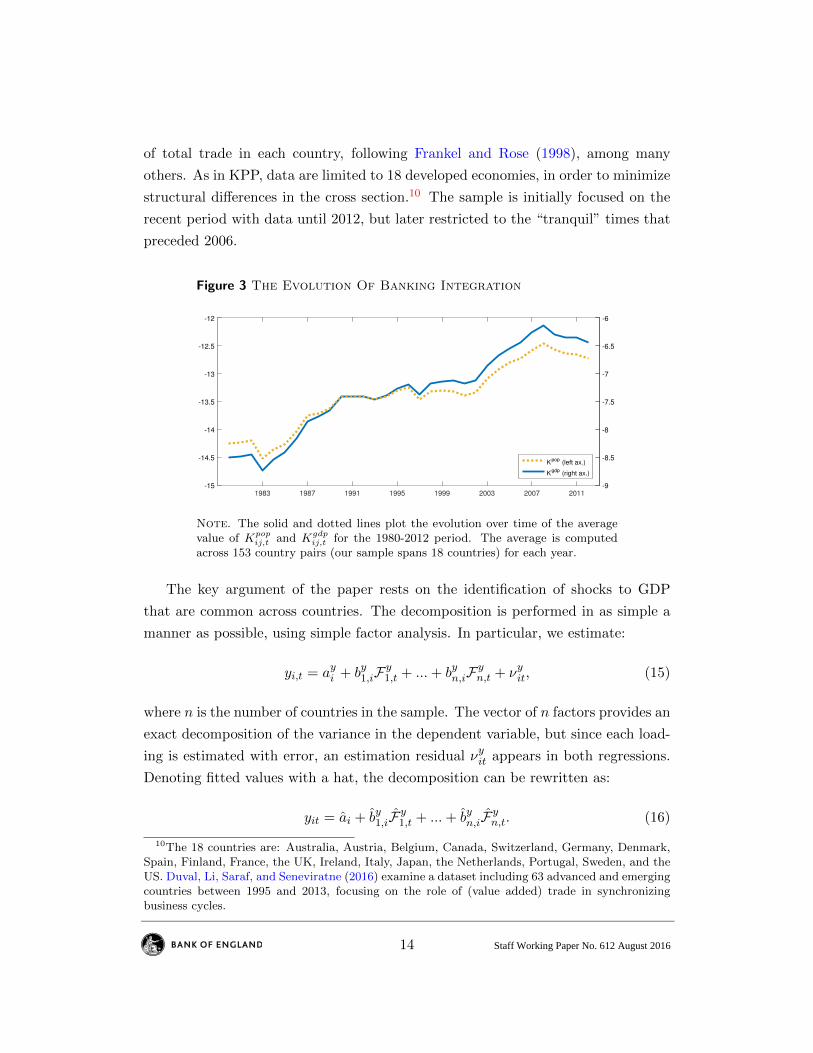
of capital holdings. Figure 3 reports the average value of Kpopij,t and Kgdp

ij,t across

country pairs. Even though both variables are normalized, an upward trend clearly

survives in both measures.

Bilateral goods trade data are collected from the IMF’s Direction of Trade data

set. The data are expressed in USD, and deflated using the US GDP deflator. Trade

intensity is measured as the ratio of bilateral exports and imports, as a proportion

13


of total trade in each country, following Frankel and Rose (1998), among many

others. As in KPP, data are limited to 18 developed economies, in order to minimize

structural differences in the cross section.10 The sample is initially focused on the

recent period with data until 2012, but later restricted to the “tranquil” times that

preceded 2006.

Figure 3 The Evolution Of Banking Integration

1983 1987 1991 1995 1999 2003 2007 2011-15

-14.5

-14

-13.5

-13

-12.5

-12

-9

-8.5

-8

-7.5

-7

-6.5

-6

Kpop

(left ax.)

Kgdp

(right ax.)

Note. The solid and dotted lines plot the evolution over time of the averagevalue of Kpop

ij,t and Kgdpij,t for the 1980-2012 period. The average is computed

across 153 country pairs (our sample spans 18 countries) for each year.

The key argument of the paper rests on the identification of shocks to GDP

that are common across countries. The decomposition is performed in as simple a

manner as possible, using simple factor analysis. In particular, we estimate:

yi,t = ayi + by1,iFy1,t + ...+ byn,iF

yn,t + νyit, (15)

where n is the number of countries in the sample. The vector of n factors provides an

exact decomposition of the variance in the dependent variable, but since each load-

ing is estimated with error, an estimation residual νyit appears in both regressions.

Denoting fitted values with a hat, the decomposition can be rewritten as:

yit = ai + by1,iFy1,t + ...+ byn,iF

yn,t. (16)

10The 18 countries are: Australia, Austria, Belgium, Canada, Switzerland, Germany, Denmark,Spain, Finland, France, the UK, Ireland, Italy, Japan, the Netherlands, Portugal, Sweden, and theUS. Duval, Li, Saraf, and Seneviratne (2016) examine a dataset including 63 advanced and emergingcountries between 1995 and 2013, focusing on the role of (value added) trade in synchronizingbusiness cycles.

14


The decomposition defines factors that may or may not be common to two or more

countries. A conventional approach to distinguish common from idiosyncratic fac-

tors is to consider the eigenvalues associated with each factor: idiosyncratic shocks

display eigenvalues strictly below one, while they are above one for shocks that affect

two countries or more. Since by construction, the eigenvalues associated with Fyk,tdecrease in k, this provides a decomposition of factors into ones that are common

to two countries or more, and ones that are specific to one single economy.

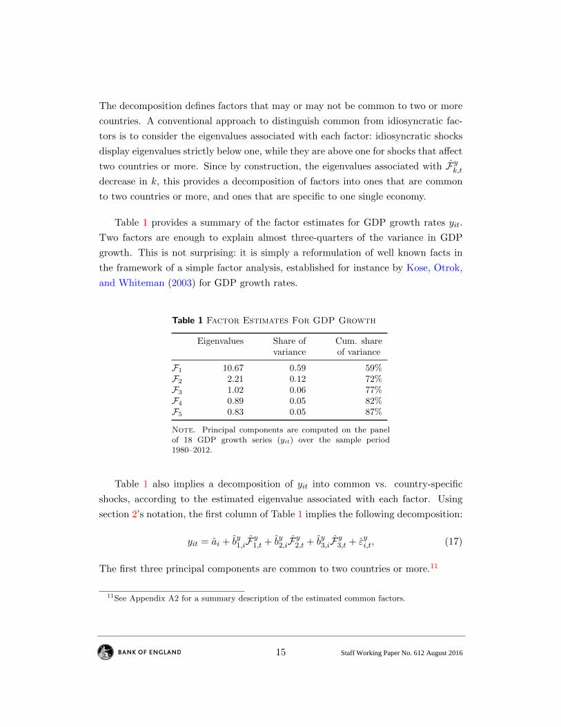
Table 1 provides a summary of the factor estimates for GDP growth rates yit.

Two factors are enough to explain almost three-quarters of the variance in GDP

growth. This is not surprising: it is simply a reformulation of well known facts in

the framework of a simple factor analysis, established for instance by Kose, Otrok,

and Whiteman (2003) for GDP growth rates.

Table 1 Factor Estimates For GDP Growth

Eigenvalues Share of Cum. sharevariance of variance

F1 10.67 0.59 59%F2 2.21 0.12 72%F3 1.02 0.06 77%F4 0.89 0.05 82%F5 0.83 0.05 87%

Note. Principal components are computed on the panelof 18 GDP growth series (yit) over the sample period1980–2012.

Table 1 also implies a decomposition of yit into common vs. country-specific

shocks, according to the estimated eigenvalue associated with each factor. Using

section 2’s notation, the first column of Table 1 implies the following decomposition:

yit = ai + by1,iFy1,t + by2,iF

y2,t + by3,iF

y3,t + εyi,t, (17)

The first three principal components are common to two countries or more.11

11See Appendix A2 for a summary description of the estimated common factors.

15


3.2 Estimation results

Equation (8) is the paper’s key panel regression. We use the principal component

decomposition just described to run three versions of the estimation. The first

simply reproduces known results, where the dependent variable is given by Sij,t that

embeds both common and idiosyncratic shocks. The two alternative specifications

condition the estimation on one kind of shock only: on common shocks only, with

SFij,t as the dependent variable, and on idiosyncratic shocks only, with Sεij,t as the

dependent variable. All three estimations are performed for the two variants of Kij,t,

normalized by population or by GDP.

Table 2 abstracts from country-pair fixed effects, and estimates β on the cross-

sectional dimension of the data, between country pairs.

Table 2 Banking Integration and Business Cycle Synchronization:Cross-sectional (“Between”) Estimates

S SF Sε S SF Sε

(1) (2) (3) (4) (5) (6)

Banking / Pop. (Kpop) 0.095 0.106 0.038(0.011) (0.008) (0.007)

[8.70] [12.85] [5.43]Banking / GDP (Kgdp) 0.091 0.082 0.049

(0.010) (0.007) (0.006)[9.52] [11.31] [7.98]

Observations 4863 4863 4863 4863 4863 4863R2 0.092 0.176 0.121 0.095 0.170 0.127Country Pairs 153 153 153 153 153 153

Note. All regression specifications include a vector of year fixed effects. Estimation isperformed over the 1980-2012 period.

The estimates are systematically positive, confirming the positive association

between finance and synchronization on average. As argued by KPP, caution is in

order in interpreting this result if there exist permanent reasons why country pairs

display high cycle synchronization and high financial integration, such as the prac-

tice of a common language, geographic proximity, or common institutions. Hence

allowances for country pair effects, αij , are of the essence.

16


Table 3 reports the panel estimates of equation (8) allowing for fixed effects. Ta-

ble 4 includes a control for the intensity of bilateral trade. In both tables, columns

(1) and (4) reproduce the significantly negative estimates of β within country pair,

as in KPP. There are permanent reasons why financial links are intense between syn-

chronized economies, captured by αij in equation (8); but once these are accounted

for, a change in financial integration tends to be associated with lower values of

Sij,t.12

Table 3 Banking Integration and Business Cycle Synchronization:Panel (“Within”) Estimates

S SF Sε S SF Sε

(1) (2) (3) (4) (5) (6)

Banking / Pop. (Kpop) -0.144 -0.154 0.075(0.040) (0.030) (0.021)[-3.63] [-5.05] [3.54]

Banking / GDP (Kgdp) -0.148 -0.159 0.072(0.042) (0.032) (0.022)[-3.56] [-4.98] [3.28]


Note. All regression specifications include a vector of country-pair fixed effects and avector of year fixed effects. Estimation is performed over the 1980-2012 period. Standarderrors are adjusted for country-pair-level heteroskedasticity and autocorrelation.

However, as this paper has argued, Sij,t embeds the heterogeneous responses of

GDP to common shocks. Inasmuch as common shocks also affect Kij,t, negative

estimates of β in columns (1) and (4) could still arise because of features specific

to each country pair: the responses of Sij,t and Kij,t to common shocks. Columns

(2) and (5) in both tables confirm that negative estimates of β arise when synchro-

nization is conditioned on common shocks only, as in equation (10). As argued in

section 2, this result could be driven by a systematic correlation between byi − byj

and bKij .

Columns (3) and (6) of Tables 3 and 4 show that the estimates of β are signif-

icantly positive when synchronization is measured by Sεij,t as in equation (6). The

12Estimates of β continue to be significantly negative if the dependent variable is SFij,t+ Sεij,tinstead of Sij,t. These results are available upon request.

17


Table 4 Banking Integration and Business Cycle Synchronization:Panel (“Within”) Estimates With Controls

S SF Sε S SF Sε

(1) (2) (3) (4) (5) (6)

Banking / Pop. (Kpop) -0.102 -0.132 0.060(0.040) (0.028) (0.024)[-2.57] [-4.71] [2.55]

Banking / GDP (Kgdp) -0.106 -0.137 0.056(0.041) (0.029) (0.024)[-2.55] [-4.65] [2.32]

Trade -0.382 -0.198 0.132 -0.386 -0.203 0.141(0.134) (0.114) (0.078) (0.133) (0.113) (0.078)[-2.86] [-1.75] [1.69] [-2.90] [-1.79] [1.81]



synchronization measure captures the equilibrium response of GDP in countries i

and j to a country-specific shock: this is the object that models of the international

business cycle have ambiguous predictions about. The contagious consequences of fi-

nance mirrored by positive estimates of β are consistent with models where financial

flows serve to alleviate binding constraints, rather than to chase high returns.

In the previous section we showed analytically that negative estimates of β and

βF arise when the elasticities of GDP and capital to common shocks are system-

atically related. This means that high byi countries should also display high bKij .

Figure 4 plots the estimates of by1,i against bK1,i, where bK1,i is the first factor load-

ing of country i’s capital, computed as Ki,t =∑

jKij,t. The correlation is positive

and significant, with inelastic countries on both counts like Australia, Japan, and

Portugal, and elastic countries on both counts, like the US and most of continental

Europe.13

13Elasticities of GDP correlate negatively with a measure of remoteness: byi tend to take signif-icantly lower values for countries that are far from the gravity center of world trade, a measureborrowed from Bravo-Ortega and di Giovanni (2006). The coefficient estimate is −1.14, with at-statistic of −4.00.

18


Figure 4 Correlation Between Factor Loadings On GDP AndCapital

USA

GBR

AUT BEL

DNK FRA

DEU ITA

NLD

SWE

CHE

CAN JPN

FIN

IRL

PRT

ESP

AUS

0.00

0.05

0.10

0.15

0.20

0.25

0.30

0.10 0.15 0.20 0.25 0.30

Capital L

oadin

g

GDP Loading

y = 0.04 + 0.78 x [0.4] [1.9]

Note. On the horizontal axis is the loading on GDP (by1,i). On the vertical axis

is the loading on capital bK1,i, where bK1,i is the first factor loading of country i’scapital, computed as Ki,t =

∑j

Kij,t. The slope and the constant of the fitted

line are reported together with t-statistics in square brackets.

One possible interpretation of such a positive correlation between by1,i and bK1,i is

that capital should go from countries with inelastic GDP to countries with elastic

GDP in periods of global (or regional) booms, and the other way round for negative

common shocks. That is: capital flows are procyclical, as it is well documented in

the literature (see, among others, Kaminsky, Reinhart, and Vegh, 2005, Rey, 2013,

Broner, Didier, Erce, and Schmukler, 2013, Bruno and Shin, 2015).. This would

account for the positive correlation between GDP and capital loadings in Figure 4.

Figure 5 explores the empirical validity of this interpretation by plotting the

cross-section of by1,i against measures of the changes in net bank holdings as per

the BIS data. We compute the average change in net bank holdings, computed for

positive or negative values of Fyt . Define:

KNET+i =

∑Fyt >0

∆t

∑j

ln (Aji,t + Lij,t)− ln (Aij,t + Lji,t)

, (18)

and:

KNET−i =∑Fyt <0

∆t

∑j

ln (Aji,t + Lij,t)− ln (Aij,t + Lji,t)

, (19)

19


where ∆t[X] denotes the first difference of variable X.

Panel (a) of Figure 5 plots the estimates of by1,i against the average change in

net bank holdings computed for positive values of Fyt (i.e., KNET+i ).

Figure 5 Correlation Between Loadings On GDP And Average ChangesIn Net Bank Holdings

USA

GBR

AUT BEL

DNK FRA

DEU

ITA

NLD

SWE

CHE

CAN

JPN

FIN

IRL

PRT

ESP

AUS

-0.08

-0.06

-0.04

-0.02

0.00

0.02

0.04

0.06

0.10 0.15 0.20 0.25 0.30

Avera

ge c

hange in n

et

bank h

old

ing

GDP Loading

(a) Ft > 0

y = -0.08 + 0.33 x [-2.3] [2.0]

USA

GBR

AUT

BEL

DNK FRA

DEU ITA NLD

SWE

CHE

CAN

JPN

FIN IRL

PRT

ESP

AUS

-0.05

-0.04

-0.03

-0.02

-0.01

0.00

0.01

0.02

0.03

0.04

0.05

0.10 0.15 0.20 0.25 0.30

Avera

ge c

hange in n

et

bank h

old

ing

GDP Loading

(b) Ft < 0

y = 0.03 - 0.18 x [1.4] [-1.7]

Note. On the horizontal axis is the loading on GDP (by1,i). On the vertical axis is the

change in net bank holdings averaged over periods when Ft > 0 (KNET+i ), in panel (a);

and when Ft < 0 (KNET−i ), in panel (b). The slope and the constant of the fitted lineare reported together with t-statistics in square brackets.

A significantly positive correlation exists, which means that on average net cap-

ital increases in countries whose GDP is responsive to common shocks in times of

global (or regional) booms. Panel (b) of Figure 5 plots the estimates of by1,i against

KNET−i . A negative relation exists, though it is only weakly significant. There

is some tendency for net capital to fall in countries with elastic GDP in times of

global (or regional) recessions, but it is less clear cut than the opposite in booms.

Taken together, Figure 5 suggests that (bank) capital tends to flow between coun-

tries with different loadings on GDP: from low byi to high byj in times of booms, and,

to a smaller extent, the opposite in times of recessions. This drives a systematic

correlation between by1,i and bK1,i, creates negative estimates of βF , and ultimately of

β. But this tends to always happen between the same countries.14

14Of course, all the results here depend on the empirical heterogeneity in byi and bKi , and theirempirical correlation across countries. Nothing guarantees that what this paper uncovers shouldhold universally. For instance, Morgan, Rime, and Strahan (2004) find estimates of β are positivein a similar estimation performed across US states between 1976 and 1994. That could reflect therelative homogeneity of US States, so that Sεij,t is well captured by Sij,t. A contrario, the negative

20


The panel of GDP growth rates used until now include the Great Recession years,

until 2012. Arguably, the most recent period includes years when financial linkages

may have been especially contagious. For instance Kalemli-Ozcan, Papaioannou,

and Perri (2013) show that estimates of β become less negative if the crisis years are

included. They explain the instability in coefficient estimates with the prevalence

of credit shocks during the Great Recession. Given the magnitude and globality of

the Great Recession, it is likely to affect estimates of common shocks, and thus the

estimated elasticities of GDP and capital to common shocks.

Table 5 repeats the previous three estimations, but on a sample that now stops

in 2006.15 Estimates of β continue to be negative when the dependent variable

is Sij,t or SFij,t; and to be positive when it is Sεij,t, consistent with the prevalence

of contagious shocks, and perhaps of credit constraints, in the years preceding the

Great Recession.

Table 5 Banking Integration and Business Cycle Synchronization:Panel (“Within”) Estimates Excluding The Great Recession Years

S SF Sε S SF Sε

(1) (2) (3) (4) (5) (6)

Banking / Pop. (Kpop) -0.280 -0.314 0.091(0.063) (0.052) (0.028)[-4.46] [-6.04] [3.22]

Banking / GDP (Kgdp) -0.284 -0.321 0.085(0.066) (0.054) (0.029)[-4.33] [-5.91] [2.91]



Endogeneity is an obvious concern for OLS estimates of equation (8). There is

every reason to expect that financial linkages, especially bank linkages, are governed

by a diversification motive. Then Kij,t tends to take high values between countries

estimates of β in Duval, Li, Saraf, and Seneviratne (2016) could arise from the large heterogeneityin a sample formed by 63 countries at various levels of development.

15Appendix A3 provides the detailed factor estimates for the 1980-2006 sample.

21


that are out of sync, i.e., where Sij,t takes large negative values. This endogeneity

bias results in estimates of β that are biased downwards: (negative) OLS estimates in

columns (1)-(2) and (3)-(5) are biased away from zero, and (positive) OLS estimates

in columns (3) and (6) are biased towards zero.

An important contribution of KPP is the introduction of an instrument for Kij,t

that is time-varying, and country pair specific. The instrument builds from the

existence of European directives, issued by the European Commission at a certain

date, and implemented later in member countries, with lags that vary with each

country. KPP focus on the 27 directives that pertain to financial regulation, as

part of the Financial Services Action Plan launched in 1998 to remove barriers

across Europe. At each point in time, and for each country pair they consider the

overlap in directives that happen to be implemented in both countries i and j. They

argue implementation dates are exogenous to current economic conditions, so that

the instrument satisfies standard excludability constraints. The index constitutes a

novel and powerful instrument for financial integration Kij,t.16

Table 6 Banking Integration and Business Cycle Synchronization:Panel (“Within”) IV Estimates Excluding The Great Recession Years

S SF Sε S SF Sε

(1) (2) (3) (4) (5) (6)

Banking / Pop. (Kpop) -0.487 -0.367 0.237(0.132) (0.084) (0.089)[-3.69] [-4.35] [2.66]

Banking / GDP (Kgdp) -0.519 -0.391 0.253(0.141) (0.090) (0.095)[-3.69] [-4.35] [2.66]



Table 6 presents Instrumental Variable estimations of equation (8), once again

for the three considered measures of cycle synchronization, Sij,t, SFij,t, and Sεij,t.16Following KPP, the instrument takes value zero for non EU member countries, and for all years

before 1998.

22


Estimates of β are still significantly negative for the measures of synchronization that

embed common shocks, Sij,t and SFij,t. As in Table 5, when synchronization focuses

on idiosyncratic shocks (i.e., when using Sεij,t as a dependent variable) estimates of

β are positive and significant.

4 Extensions

This section discusses two extensions to our baseline specification. First, we con-

sider an alternative measure of synchronization, namely the Pearson correlation

coefficient. Second, we consider the possibility that our estimated factor loadings

vary over time.

4.1 Correlation Coefficients

The measure of cycle synchronization used in most of the literature until recently is

the Pearson correlation coefficient. It is problematic in panel regressions, because

it is measured with error and because it responds to changes in the variance of

the underlying shocks. Still, KPP show that the negative estimates in equation (8)

survive this alternative measurement of synchronization.

Consider the consequences of equation (4) on the Pearson correlation ρij between

the GDP growth rates of countries i and j. By definition:

ρij =(wFi) 1

2(wFj) 1

2 +(1− wFi

) 12(1− wFj

) 12 ρεij , (20)

where wFi =b2i V (Fyt )V (yi,t)

is the share of the variance of GDP growth in country i that

corresponds to common shocks, and ρεij is the Pearson correlation coefficient that

captures cycle synchronization conditional on idiosyncratic shocks. As is evident, in

the presence of common shocks, the Pearson correlation between GDP growth is an

imperfect measure of the actual correlation coefficient implied by country-specific

shocks, even if underlying risk is held constant. A corrective term drives a wedge

between the two coefficients. Its magnitude depends on the share of the variance in

GDP growth that can be explained by common shocks in both countries i and j.

Correlation coefficients were traditionally used in cross-section, since they are

computed in the time dimension. But it is also possible to compute them over

23


successive sub-periods, and use the resulting panel as the dependent variable in

equation (8). Then the corrective term in equation (20) involving wFi and wFj can

also be time-varying. With an intuition that is analogous to Forbes and Rigobon

(2002), changes in the variance of the underlying shocks affect the panel properties

of ρij . The empirical question posed by this possibility is whether the estimates of

β in equation (8) depend on how synchronization is measured, by ρij or by ρεij .

Table 7 shows that it does: the estimates of β are negative and borderline signifi-

cant in columns (1) and (4), when the dependent variable in equation (8) is given by

ρij,t, computed over five-year windows. It becomes strongly negative and significant

when the correlation coefficient is computed on common shocks only, in columns (2)

and (5). But it is essentially zero when the dependent variable is replaced by ρεij,t.

We note that Pearson correlation coefficients are estimated over five-year windows

in table 7, and constitute therefore measures of synchronization that are estimated

with considerable error. We note furthermore that changes over time in both ρij,t

and ρεij,t continue to be affected by changes in the variances of the underlying shocks.

While it is reassuring that the Pearson correlation coefficient conditioned on common

shocks continues to be negatively related with financial integration, it is not overly

worrisome that the relation between ρεij,t and financial integration is essentially zero:

there are many well known reasons why this may happen.

Table 7 Banking Integration and Business Cycle Synchronization:Panel (“Within”) Estimates – Pearson Correlation Coefficient

ρ ρF ρε ρ ρF ρε

(1) (2) (3) (4) (5) (6)

Banking / Pop. (Kpop) -0.102 -0.031 -0.017(0.061) (0.015) (0.020)[-1.67] [-2.07] [-0.83]

Banking / GDP (Kgdp) -0.110 -0.033 -0.018(0.064) (0.016) (0.021)[-1.74] [-2.11] [-0.85]



24


4.2 Time-Varying Factor Loadings

During the estimation period we consider (1980-2012) global goods and financial

markets have grown at fast pace as countries integrated. One would think the

responsiveness of countries to global developments is likely to have changed, as well.

In this section we address this possibility, by estimating a model where country-

specific factor loadings are allowed to vary over time.

Consider a version of equation (4) where factor loadings are allowed to be time-

varying:

yt = ayt + bytFyt + eyt , (21)

where, for ease of notation, the country subscripts i are ignored. Assume that the

coefficients ayt and byt evolve as random walks. In state-space form this model can

be expressed as:

yt = Xtβt + eyt . (22)

βt = βt−1 + vt (23)

where Xt = (1,Fyt ), βt = (ayt , byt )′, and V ar(eyt ) = R and V ar(vt) = Q.

The model (22)-(23) can be easily estimated via Gibbs sampling (see Blake and

Mumtaz, 2012). Specifically, if the time-varying coefficients βt are known, then the

conditional posterior distribution of R is inverse Gamma, and the distribution of Q

is inverse Wishart. Conditional on R and Q the model (22)-(23) is a linear Gaussian

state space model. Since the conditional posterior of βt is normal, the mean and

the variance of βt can be derived with the Kalman filter.17

Figure 6 compares time-varying estimates to their static equivalent for the 18

countries in the sample. While some variation is apparent, time-varying estimates

of factor loadings are rarely significantly different from their constant counterparts.

17Appendix B provides the details on the Gibbs sampling algorithm, initial conditions and priors.

25


Figure 6 Time-varying Estimates Of The Loadings On The First Prin-cipal Component

United States

1986 1992 1998 2004 2010

0.1

0.15

0.2

0.25

United Kingdom

1986 1992 1998 2004 2010

0.1

0.2

0.3

Austria

1986 1992 1998 2004 2010

0.1

0.2

0.3

Belgium

1986 1992 1998 2004 2010

0.2

0.3

0.4

Denmark

1986 1992 1998 2004 2010

0

0.2

0.4France

1986 1992 1998 2004 2010

0.1

0.2

0.3

0.4

Germany

1986 1992 1998 2004 2010

0.1

0.2

0.3

Italy

1986 1992 1998 2004 2010

0.1

0.2

0.3

Netherlands

1986 1992 1998 2004 2010

0.1

0.2

0.3

Sweden

1986 1992 1998 2004 2010

0.1

0.2

0.3

0.4

Switzerland

1986 1992 1998 2004 2010

0.1

0.2

0.3

0.4Canada

1986 1992 1998 2004 2010

0.1

0.2

0.3

Japan

1986 1992 1998 2004 2010

0

0.2

0.4

Finland

1986 1992 1998 2004 20100

0.2

0.4

Ireland

1986 1992 1998 2004 2010

0.1

0.2

0.3

Portugal

1986 1992 1998 2004 2010

0.1

0.2

0.3

0.4

Spain

1986 1992 1998 2004 2010

0.1

0.2

0.3

Australia

1986 1992 1998 2004 2010

0

0.1

0.2

Time-varying 16/84 Percentile Fixed (OLS)

Note. Median estimates of the time-varying parameters (solid line) in model (22)-(23).Shaded areas display the 68 percent credible intervals. The dashed line reports the OLSfixed estimates.

26


Table 8 reports the results implied when the time-varying estimates of byt are used

to decompose Sij,t into SFij,t, and Sεij,t. The estimates of β continue to switch signs

as in the results presented above: negative when Sij,t or SFij,t are the dependent

variable, but positive and significant when Sεij,t is. This provides an alternative

decomposition where the existence of common shocks obscures the effect of finance

on synchronization.

Table 8 Banking Integration and Business Cycle Synchronization:Panel (“Within”) Time-Varying Parameter Estimates

S SF Sε S SF Sε

(1) (2) (3) (4) (5) (6)

Banking / Pop. -0.144 -0.195 0.033(0.040) (0.037) (0.012)[-3.63] [-5.21] [2.68]

Banking / GDP -0.148 -0.199 0.031(0.042) (0.040) (0.013)[-3.56] [-5.03] [2.46]



5 Conclusion

In the workhorse model of international real business cycles with complete markets,

financial flows exacerbate asymmetries in business cycles as they relocate efficiently

to the country with highest marginal product of capital. Under mild heterogeneity

(e.g., in factor shares) the same model has observationally equivalent predictions

in response to a common shock: while productivity changes are identical in both

countries, the marginal products of capital respond differently, and so do GDP

growth rates. The key difference is interpretation: with common shocks, capital

flows respond to countries’ fundamental heterogeneity, rather than an efficient quest

for high returns.

27


To establish whether international capital flows are fundamentally efficient, it is

therefore imperative to control for common shocks of a specific kind: those that are

allowed to have heterogeneous effects across countries. Conditional on such common

shocks, we find that financial linkages tend to result in less synchronized business

cycles in 18 OECD countries. We show this finding is driven by a permanent fea-

ture of cross-country heterogeneity (i.e., a systematic correlation between capital

flows and countries’ GDP elasticity to common shocks), rather than by random,

country-specific shocks. In contrast, conditional on well identified idiosyncratic,

country-specific shocks we show that financial flows result in more synchronized

business cycles in the vast majority of specifications. This finding provides sup-

port for the possibility that international financial flows serve to alleviate binding

financial constraints, thus fostering contagion.

28


References

Allen, F., and D. Gale (2000): “Financial Contagion,” Journal of Political Economy,108(1), 1–33.

Backus, D. K., P. J. Kehoe, and F. E. Kydland (1992): “International Real BusinessCycles,” Journal of Political Economy, 100(4), 745–75.

Baxter, M., and M. A. Kouparitsas (2005): “Determinants of business cycle comove-ment: a robust analysis,” Journal of Monetary Economics, 52(1), 113–157.

Bernanke, B., J. Boivin, and P. S. Eliasz (2005): “Measuring the Effects of MonetaryPolicy: A Factor-augmented Vector Autoregressive (FAVAR) Approach,” The QuarterlyJournal of Economics, 120(1), 387–422.

Blake, A., and H. Mumtaz (2012): Applied Bayesian econometrics for central bankers,no. 4 in Technical Books. Centre for Central Banking Studies, Bank of England.

Bravo-Ortega, C., and J. di Giovanni (2006): “Remoteness and Real Exchange RateVolatility,” IMF Staff Papers, 53(si), 6.

Broner, F., T. Didier, A. Erce, and S. L. Schmukler (2013): “Gross capital flows:Dynamics and crises,” Journal of Monetary Economics, 60(1), 113–133.

Bruno, V., and H. S. Shin (2014): “Cross-border banking and global liquidity,” BISWorking Papers 458, Bank for International Settlements.

(2015): “Cross-Border Banking and Global Liquidity,” Review of Economic Stud-ies, 82(2), 535–564.

Caselli, F. (2005): “Accounting for Cross-Country Income Differences,” in Handbook ofEconomic Growth, ed. by P. Aghion, and S. Durlauf, vol. 1 of Handbook of EconomicGrowth, chap. 9, pp. 679–741. Elsevier.

Corsetti, G., M. Pericoli, and M. Sbracia (2005): “’Some contagion, some interde-pendence’: More pitfalls in tests of financial contagion,” Journal of International Moneyand Finance, 24(8), 1177–1199.

Crucini, M., A. Kose, and C. Otrok (2011): “What are the driving forces of interna-tional business cycles?,” Review of Economic Dynamics, 14(1), 156–175.

Dedola, L., and G. Lombardo (2012): “Financial frictions, financial integration and theinternational propagation of shocks,” Economic Policy, 27(70), 319–359.

Devereux, M. B., and J. Yetman (2010): “Leverage Constraints and the InternationalTransmission of Shocks,” Journal of Money, Credit and Banking, 42(s1), 71–105.

Devereux, M. B., and C. Yu (2014): “International Financial Integration and CrisisContagion,” NBER Working Papers 20526, National Bureau of Economic Research, Inc.

Doyle, B. M., and J. Faust (2005): “Breaks in the Variability and Comovement of G-7Economic Growth,” The Review of Economics and Statistics, 87(4), 721–740.

29


Duval, R., N. Li, R. Saraf, and D. Seneviratne (2016): “Value-added trade andbusiness cycle synchronization,” Journal of International Economics, 99(C), 251–262.

Forbes, K. J., and R. Rigobon (2002): “No Contagion, Only Interdependence: Measur-ing Stock Market Comovements,” Journal of Finance, 57(5), 2223–2261.

Forbes, K. J., and F. E. Warnock (2012): “Capital flow waves: Surges, stops, flight,and retrenchment,” Journal of International Economics, 88(2), 235–251.

Forni, M., and L. Reichlin (1998): “Let’s Get Real: A Factor Analytical Approach toDisaggregated Business Cycle Dynamics,” Review of Economic Studies, 65(3), 453–73.

Frankel, J. A., and A. K. Rose (1998): “The Endogeneity of the Optimum CurrencyArea Criteria,” Economic Journal, 108(449), 1009–25.

Giannone, D., M. Lenza, and L. Reichlin (2010): “Business Cycles in the Euro Area,”in Europe and the Euro, NBER Chapters, pp. 141–167. National Bureau of EconomicResearch, Inc.

Hirata, H., M. A. Kose, and C. Otrok (2013): “Regionalization vs. Globalization,” inGlobal Interdependence, Decoupling, and Recoupling, pp. 87–130. MIT Press.

Imbs, J. (2006): “The real effects of financial integration,” Journal of International Eco-nomics, 68(2), 296–324.

IMF (2013): “Dancing Together? Spillovers, Common Shocks, and the Role of Financial andTrade Linkages,” in World Economic Outlook, October 2013, world economic outlook 3.Washington: International Monetary Fund.

Kalemli-Ozcan, S., E. Papaioannou, and F. Perri (2013): “Global banks and crisistransmission,” Journal of International Economics, 89(2), 495–510.

Kalemli-Ozcan, S., E. Papaioannou, and J.-L. Peydro (2013): “Financial Regula-tion, Financial Globalization, and the Synchronization of Economic Activity,” Journal ofFinance, 68(3), 1179–1228.

Kaminsky, G. L., C. M. Reinhart, and C. A. Vegh (2005): “When It Rains, It Pours:Procyclical Capital Flows and Macroeconomic Policies,” in NBER Macroeconomics An-nual 2004, Volume 19, NBER Chapters, pp. 11–82. National Bureau of Economic Re-search, Inc.

Kilian, L. (2008): “A Comparison of the Effects of Exogenous Oil Supply Shocks on Outputand Inflation in the G7 Countries,” Journal of the European Economic Association, 6(1),78–121.

Kose, M. A., C. Otrok, and C. H. Whiteman (2003): “International Business Cycles:World, Region, and Country-Specific Factors,” American Economic Review, 93(4), 1216–1239.

(2008): “Understanding the evolution of world business cycles,” Journal of Inter-national Economics, 75(1), 110–130.

30


Monnet, E., and D. Puy (2016): “Has Globalization Really Increased Business CycleSynchronization?,” IMF Working Papers 16/54, International Monetary Fund.

Morgan, D., B. Rime, and P. E. Strahan (2004): “Bank Integration and State BusinessCycles,” The Quarterly Journal of Economics, 119(4), 1555–1584.

Mumtaz, H., S. Simonelli, and P. Surico (2011): “International Comovements, Busi-ness Cycle and Inflation: a Historical Perspective,” Review of Economic Dynamics, 14(1),176–198.

Peersman, G., and F. Smets (2005): “The Industry Effects of Monetary Policy in theEuro Area,” Economic Journal, 115(503), 319–342.

Rey, H. (2013): “Dilemma not trilemma: the global cycle and monetary policy indepen-dence,” Proceedings - Economic Policy Symposium - Jackson Hole, pp. 1–2.

31


A Additional results

A.1 Heterogeneity in OECD Economies

Table A.1 provides the values of capital shares and depreciation rates for the coun-tries considered in our main empirical analysis. The data (from Penn World Table,version 8.1) show a high degree of heterogeneity across countries. The share ofcapital ranges from 0.28 to 0.52 and the depreciation rates from 0.34 to 0.48. Foradditional evidence on cross-country heterogeneity see Caselli (2005).

Table A.1 Cross-country Heterogeneity in CapitalShares and Depreciation Rates

Capital share (θ) Depreciation (δ)

Australia 0.37 0.040Austria 0.36 0.042Belgium 0.38 0.042Canada 0.40 0.039Denmark 0.34 0.040Finland 0.37 0.037France 0.35 0.034Germany 0.34 0.038Ireland 0.52 0.041Italy 0.42 0.041Japan 0.44 0.044Netherlands 0.36 0.038Portugal 0.32 0.046Spain 0.35 0.036Sweden 0.33 0.048Switzerland 0.28 0.048United Kingdom 0.36 0.043United States 0.36 0.039

Note. Data from Penn World Table (version 8.1). Capital share(θ) is 1 minus the share of labour compensation in GDP at currentnational prices; Depreciation (δ) is the average depreciation rate ofthe capital stock.

A.2 Principal components

We compute principal components using the pca command in Stata. In order tobe able to use the eigenvalue criterion to select the appropriate number of principalcomponents (as described in the main text), we normalize the data — so that eachcountry-specific growth rate (yit) has unit variance. Therefore we can interpret all

32


principal component with associated eigenvalues greater than 1 as common to atleast two countries.

Figure A.1 reports the estimated first three principal components (from the panelof GDP growth rates yit) that are common to 2 or more countries, together withthe annual growth rate of World GDP from IMF IFS. The principal componentapproach is a purely statistical process. While trying to understand what the first,second, or third factors capture is outside of the scope of this paper, we providesome evidence that they are all economically relevant as they are all related withglobal output growth (correlation coefficients range from 0.16 to 0.69).

Figure A.1 Estimated Principal Components and World GDPGrowth

1983 1987 1991 1995 1999 2003 2007 2011-15

-10

-5

0

5

10

PC1

PC2

PC3 World GDP

Note. Principal components are computed on the panel of 18 GDP growthseries (yit). Annual World GDP growth is from IMF International FinancialStatistics.

A.3 Factor estimates for the 1980-2006 period

Table A.2 provides a summary of the factor estimates for GDP growth rates yitover the period 1980–2006. As in the baseline sample period (that runs from 1980to 2012), the first three factors explain about 70 percent of the variance of yit.According to the eigenvalue criterion, we retain the same number of factors as inthe baseline.

33


Table A.2 Factor Estimates For GDP Growth Excluding TheGreat Recession Years

Eigenvalues Share of Cum. sharevariance of variance

F1 5.27 0.42 42%F2 2.61 0.21 63%F3 1.09 0.09 71%F4 0.91 0.07 78%F5 0.84 0.07 85%

Note. Principal components are computed on the panel of 18 GDP growthseries (yit) over the sample period 1980–2006.

B Estimation of time-varying parameters model

Consider the time-varying parameters model in (22)-(23). The Gibbs samplingalgorithm consists of the following steps:

1. Set starting values (i.e., β0, V ar (β0) , R0, Q0) and priors

P(R) ∼ IG(T02,θR

2) (B.1)

P(Q) ∼ IW(T02,θQ

2) (B.2)

2. Sample the state variable βt conditional on R and Q from its conditionalposterior distribution using the Kalman filter

3. Using β0 and V ar (β0) run Kalman Filter to get mean and variance of βt ateach point in time

4. Conditional on βt, sample Q and R from their posterior distributions.

5. Repeat steps 1 to 3 until convergence is detected.

Below we describe how we proceed in detail.

Setting β0,i, V ar(β0,i), and R0,i.

We compute a fixed parameter version of model (21) on the full sample for allcountries. Therefore, for each country i, we get an estimate of β0,i, V ar

(β0,i), and

34


R0,i:

β0 =(X ′tXt

)−1 (X ′tYt

)(B.3)

V ar (β0) = R0 ⊗(X ′tXt

)−1(B.4)

R0 =(yt −Xtβt) (yt −Xtβt)

′

(T −K)(B.5)

where T denotes the number of observations.

Setting Q0,i.Since Q0 is unobserved, one could do a rolling window OLS estimation of the

fixed parameter model to get a time-varying estimate of β0. Then, an estimate ofQ0 can be obtained by running an VAR(1) model on the rolling estimates of β0:

β0,t = Φβ0,t−1 + ξτ . (B.6)

and recovering the covariance matrix of ξt in equation (B.6) as:

Q0 =

(β0,t − Φβ0,t−1

) (β0,t − Φβ0,t−1

)′(T −K)

. (B.7)

For the above procedure to work we clearly need a large number of observations.The sample has to be large enough to allow for a rolling window estimation. Theannual frequency of our data set creates a limitation for the implementation of thestrategy. We increase the number of available observations using a quarterly dataset that is comparable to our annual data set (quarterly real GDP data from theOECD from 1980:Q1 to 2012:Q4).

We then estimate a fixed parameter version of model (21) using a rolling window.To do that, we use a window of 40 quarters.

We then estimate a VAR(1) model as in (B.6) on the rolling estimates andcompute variance-covariance Q0,i for each country.

Setting the priorsConditional on βt the posterior distribution of R is inverse Gamma and the

posterior distribution of Q is inverse Wishart:

P(R) ∼ IG(T0, θR) and P(Q) ∼ IW(T0, θ

Q). (B.8)

We set T0 = 32, i.e. the number of observations in our (annual) sample. We

then set θR so that the mean of IG(T02 ,θR

2 ) matches V ar(et) ≡ R0 and the mean

of IW(T02 ,θQ

2 ) matches V ar(vt) ≡ Q0. Therefore, for P(Ri) ∼ IG(T0,i, θRi ) we

35


set θRi = R0,i(T0,i − 1). For P(Qi) ∼ IW(T0, θQi ) we set the diagonal element

θQnn,i = Q0,i(T0 − n− 1).

ImplementationWe run 100,000 replications, discard the first 99,000, and use the remaining 1,000

draws to form the empirical distribution of the parameters of (22)-(23)

36


Bank of England Staff Working Paper No. 612

Documents

Transcript of Bank of England Staff Working Paper No. 612