Bank Branch Supply and the Unbanked Phenomenon∗

Claire Celerier † Adrien Matray ‡

First draft: March 2013

Current draft: October 17, 2016

Abstract

An exogenous increase in the density of bank branches reduces the share of unbankedhouseholds among low income populations. This finding is established using US interstatebranching deregulation between 1994 and 2010 as an exogenous shock to the entry of newbranches in poor counties. We rule out demand-based explanations for the entry of newbranches showing that branching deregulation has no effect either on a placebo sample ofnon-deregulated institutions, or on overall county economic prosperity. Using householdlevel data, we find that this exogenous supply-shock on branch density increases thelikelihood for low-income households to hold a bank account. The effect is even strongerfor populations that are more likely to be rationed by banks, such as black householdsliving in ”high racial bias” states, or for households living in rural areas where branchdensity is initially low.

Keywords : Banks, Unbanked Households, Household Finance, Discrimination

JEL codes : G21, G28, D14, D43, J15

∗We would like to thanks Giorgia Barboni, Martin Brown, Olivier Dessaint, Ralph de Haas, JeanImbs, Augustin Landier, Steven Ongena, Thomas Piketty, Jerome Pouyet, Robert Seamans, Boris Vallee,Neeltje Van Horen, Ernesto Villanueva Lopez and various seminar participants at the Banque de France,Paris School of Economics, Einaudi EIEF and the Swiss Conference on Financial Intermediation for theircomments. This paper was previously circulated under the title: “Mainstream Finance: Why don’t thePoor Participate? Evidence from Bank Branching Deregulation in the United States”.†Claire Celerier - University of Zurich, E-mail: claire.celerier@bf.uzh.ch. Claire Celerier ac-

knowledges financial support from the Swiss Finance Institute and URPP Finreg‡Adrien Matray - Princeton University

1

The fact that poor families often rely on informal means to manage their fi-

nancial lives suggests that the formal sector is not meeting their needs.

National Poverty Center, 2008

1 Introduction

There is a large debate about the reasons why so many low-income households - 35 to

45% in the United States - are unbanked, i.e., possess neither a checking nor a savings

account. One question is whether being unbanked is driven by supply- or demand-side

factors (see, for instance, Bertrand et al. (2004) or Barr and Blank (2008)). The “demand-

side” view attributes the unbanked phenomenon to cultural determinants (the poor may

distrust financial institutions or may not have a culture of saving) or to a lack of financial

literacy. Alternatively, the “supply-side” view suggests that standard bank practices

create hurdles for the poor. Minimum account balances, overdraft fees, a large distance

between branches and the proliferation of formal steps to open an account result in costs

that may be too high for poor households to manage (Washington (2006), Barr and

Blank (2008)). Furthermore, bank financial services may not be tailored to low-income

households. These two polar explanations have different policy implications. Whereas the

demand-side view predicts interventions at the household level through financial literacy

programs, for example, the supply-side view suggests that banking regulation, by giving

banks incentives to change their behavior, may reduce the share of unbanked households.

This paper shows that an exogenous increase in the density of bank offices in poor

counties has a positive impact on the share of low-income households with a bank ac-

count. To do so, we exploit interstate branching deregulation in the U.S. after 1994 as

an exogenous shock on branch entry. While the passage of the Interstate Banking and

Branching Efficiency Act (IBBEA) in 1994 made interstate branching fully legal, states

kept the right to erect barriers to the entry of interstate branches, and partially lifted

these barriers over the following years. Rice and Strahan (2010) construct a time-varying

2

index to capture these state-level differences in regulatory constraints. We combine this

index with bank office location data from the FDIC to study bank coverage and micro

data on households from the Survey of Income and Program Participation (SIPP) from

1993 to 2010 to identify low-income households with or without a bank account (Wash-

ington (2006)). The SIPP unique focus on low-income American households, coupled

with its yearly frequency, make the data particularly well suited for our analysis

We first establish the positive effect of interstate branching deregulations on the den-

sity of bank branches in poor counties. We find that the density of bank branches increases

by around 30% in poor counties after a state fully deregulates. We then ensure that this

increase is not driven by demand for credit and banking services by looking at 1) the den-

sity of credit union branches that were unaffected by the deregulation because of their

legal status and, 2) the effect of deregulations on economic activity in poor counties. We

find that branching deregulations have no effect either on the coverage of credit unions or

on personal income growth, unemployment and household leverage. The absence of effect

on the placebo sample of credit unions confirms that branching deregulation constitutes

a supply shock that does not reflect contemporaneous or expected changes in the demand

for banking services. This absence of effect of branching deregulation on county economic

prosperity makes it an ideal laboratory for our research question by allowing us to isolate

supply effects (Favara and Imbs (2015)).1

Second, we show that interstate branching deregulation is associated with a significant

drop in the rate of unbanked households among low-income populations. Figure 2 plots

the change in the likelihood of holding a bank account in the years before and after

deregulation relative to a control group of states that do not deregulate. We observe

a significant increase in the share of banked households following deregulation. Our

regressions confirm this result. The share of low income households with a bank account

increases by 4 percentage points after a state fully deregulates, which corresponds to a

1This absence of effect on county economic activity could seem surprising given the large literatureon the real effects of previous banking deregulations (Jayaratne and Strahan (1996) among others).However, all these papers explore different deregulation episodes that preceded and were completedbefore the interstate branching deregulation we are looking at. There is no reason why the real effectsobserved in earlier periods in response to different shocks would have the same effect in 1994.

3

15% increase in relative term. In all of our specifications, we control for a large number

of household covariates that capture several dimensions of income, skills and labor status

and for main state macroeconomic variables to further control for demand effects.

Third, we show that the effect of intensified bank competition is stronger for popula-

tions that are ex ante more likely to be rationed by banks, which reinforces the identifica-

tion of supply effects. First, we find that black households benefit more from branching

deregulations than do non-black households only in states with a history of discrimina-

tion. For the same level of income, black households are indeed 20% less likely than white

households to hold a bank account in states with a history of discrimination, but this gap

narrows to only 15% after deregulation, to the level observed in states with no history

of discrimination. Second, the effect of branching deregulations increases when the level

of income decreases. Whereas branching deregulations have no significant impact for

middle-income households, whose income is above twice the poverty line, deregulating

results on average in a 4 percentage points increase in the probability of holding a bank

account among low-income households, and the effect increases up to 6 percentage points

for poor households, whose income is below the poverty line. Third, the magnitude of the

effect is significantly larger for households living in rural areas, where branch coverage is

lower ex ante. Finally, we differentiate between households with lower and higher levels

of education. We find that the effect of deregulation is stronger for more educated house-

holds. For these households, being unbanked is less likely to be driven by sophistication

because they have relatively higher financial literacy (Lusardi and Mitchell (2007)).

Finally, we show that having access to bank accounts improves wealth accumulation

but does not translate into higher levels of indebtedness. First, deregulation increases

the share of low-income households with interest-earning assets in both banks and other

financial institutions. Second, we show that deregulation impacts neither the probability

to own debt nor the debt to income ratio of low income households, which mitigates the

fear that banking competition fosters “predatory lending”.

Our paper contributes to the literature on the determinants of being unbanked. This

literature has been scarce mainly as a result of the challenge of disentangling demand-side

4

from supply-side factors (see Barr and Blank (2008) for a broad survey of the literature).

Socio-economic characteristics, which may capture both demand- or supply-side effects,

are often noted as the most influential determinants of holding a bank account (Rhine

et al. (2006), Barr (2005), Barr et al. (2011), Hogarth and O’Donnell (1999)). On the

demand side, Kearney et al. (2010) and Cole et al. (2016) show that by offering a savings

account with lottery-like features, banks can motivate the opening of savings accounts.

This paper provides evidence consistent with the literature showing that geographic prox-

imity matters, even more for low income households (Nguyen (2014)). The debate on

the determinants of being unbanked also raises the question of the role played by the de-

velopment of alternative financial services (see, for instance, Morgan and Strain (2008),

Melzer (2011), Bertrand and Morse (2011), Morse (2011), Morgan et al. (2012), Carrell

and Zinman (2014)).

More generally, our paper relates to the literature that shows the large and positive

effect of access to banking accounts on savings rates (Ashraf et al. (2006), Schaner (2013)),

on investment in preventative health (Dupas and Robinson (2013b)) and in education

(Prina (2014)), and on starting a business (Dupas and Robinson (2013a)). Holding a

bank account can also protect households from predatory lending.

Finally, our paper adds to the literature that evaluates the effect of intensified compe-

tition on racial or gender discrimination. Increased competition has been found to reduce

the black-white wage gap in the trucking industry (Peoples and Talley (2001)), in the

economy overall (Levine et al. (2013)) and between genders (Black and Strahan (2001)).

Our results are also in line with Chatterji and Seamans (2012), who shows that credit

card deregulation expanded access to credit, particularly among blacks.2

The rest of the paper proceeds as follows. Section 2 explains the data and the empirical

strategy. Section 3 presents the empirical strategy and the results on branch entry.

Section 4 presents the results on household-level data. Section 5 runs various robustness

checks. Section 6 concludes.

2However, as shown by Ouazad and Ranciere (2013), the relaxation of credit standards can also leadto more black segregation by giving white households the opportunity to relocate in white neighborhoods.

5

2 Data

2.1 Banking Deregulation

Restrictions on interstate banking and branching have their historical roots in the 1789

Constitution (Johnson and Rice (2008)).3 Although the Constitution prevented states

from issuing fiat money and taxing interstate commerce, it gave them the right to char-

ter and regulate banks. Since then, states have used banks as a source of revenue by

charging fees for granting charters, levying taxes and owning shares. These revenues

have given states incentives to restrict competition from out-of-state banks and to create

local monopolies. In 1927, the McFadden Act implicitly prohibited interstate branching

by commercial banks. In the following years, however, bank holding companies were

created to circumvent the law and they acquired branches across states. In 1956, the

Bank Holding Company Act ended this development, preventing banks from acquiring

banks or branches outside their state unless the state of the targeted bank permitted such

acquisitions. The first step toward interstate banking came in 1978 when Maine began to

allow out-of-state bank holding companies to acquire banks on a reciprocal basis. Other

states followed beginning in 1982, but interstate branching was still not allowed until

1994.

In 1994, the Interstate Banking and Branching Efficiency Act (IBBEA), also known as

the Riegel-Neal Act, effectively permitted bank holding companies to enter other states

and operate branches. However, it also allowed states to erect barriers to out-of-state

entry with regard to four dimensions: (i) the minimum age of the targeted bank (5 years,

3 years or less), (ii) de-novo branching without an explicit agreement by state authorities,

(iii) the acquisition of individual branches without acquiring the entire bank and (iv) a

statewide deposit cap, that is, the total amount of statewide deposits controlled by a

single bank or bank holding company. Following the passage of the IBBEA in 1997,

states had the opportunity to modify each of these provisions, and many states did so.

3Interstate banking refers to the control by bank holding companies of banks across state lines,whereas interstate branching means that a single bank may operate branches in more than one statewithout requiring separate capital and corporate structures for each state.

6

In fact, 43 states have relaxed the protection of their banking market since then.

Following Rice and Strahan (2010), we construct a deregulation index that ranges

from 0 to 4 to capture each dimension of state-level branching restrictions: 0 for fully

regulated and 4 for fully deregulated states. Therefore, an increase in the index value

implies greater competition.4

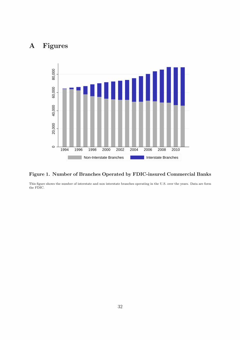
Interstate branching deregulation has fostered the development of multi-state banking.

As Figure 1 shows, not only has the total number of branches increased since 1994, but

each local market has also experienced a strong penetration of “out-of-state” branches,

which have challenged local incumbents. Analyzing the other dimension of IBBEA, the

interstate banking deregulation, Dick (2006) finds that it has translated into a dramatic

decrease in the number of regional dominant banks and a slight increase in the number

of small banks, resulting in a strong appreciation of bank density.

INSERT FIGURE 1

2.2 Household Data

Data on households comes from the SIPP and covers the 1993-2010 period. The SIPP

is a running panel that collects detailed information about income and demographics

for 20,000 to 30,000 households over 2 to 3 years. Most importantly, the SIPP includes

topical modules focusing on household asset allocation and the use of banking services.

We exploit the data from these topical modules to create a dummy variable BankAccount

that takes the value 1 if at least one member in the household holds either a free checking

or savings account, and 0 otherwise. The large size of the sample allows us to focus on

low-income households, i.e., those below 200% of the poverty threshold, which is key for

our analysis because low-income households are more likely to be rationed by banks.5

We work at the household rather than the individual level because households often pool

4We reverse Rice and Strahan (2010)’s index to facilitate the description of our results. The indextakes the value 4 before the deregulation year.

5The poverty threshold is defined in the SIPP and varies with the number of adults and children inthe household and, for some household types, the age of the household head.

7

resources; a bank account in one member’s name can provide access to banking services

to other members of the same household. We collapse each household observation at the

year level. This leaves us with a total sample of 135,524 low-income households living in

45 states plus the District of Columbia over the 1993-2010 period.6

Finally, we exploit the very detailed information on socio-demographics that the SIPP

provides to control for a large set of variables in our identification strategy. These controls

include family type (size of the households, whether the household head is single and

female, and whether the head is married), the socio-demographic characteristics of the

head of household (age, race, three dummies for education: elementary, high school or

college degree, employment status) and the household’s economic characteristics (monthly

income, dummy for receiving social security, dummy for transfer income).

Based on the SIPP data, we find that 36.3% of low-income households are unbanked

in 1993. This rate increases up to more than 40% in 2002. We observe the same in-

creasing trend in the Panel Study of Income Dynamics data (Table A.3). One potential

explanation would be the rapid development of alternative financial services over this

period. The 2011 National Survey of Unbanked and Underbanked Households from the

FDIC indicates that the proportion of unbanked households has also increased slightly

during the recent financial crisis.7

Table 1 shows the summary statistics for banked and unbanked households in our

sample. On average, banked households are less likely to be black and to receive transfer

income and are richer than unbanked households.

INSERT TABLE 1

2.3 County-Level Data

Bank and Credit Union Location Data

6To ensure the confidentiality of the data, the SIPP aggregates five states in two groups. These statesare: Maine and Vermont (first group) and North Dakota, South Dakota and Wyoming (second group),this explains why we do not have 50 +1 states. Unfortunately, there is a gap in the data between 2006and 2008 because no topical module on asset allocation was administered during these years.

7http://www.fdic.gov/householdsurvey/

8

Both data on bank branch location and deposit holdings come from the Sum of De-

posits (SOD) maintained by the Federal Deposit Insurance Fund (FDIC). The FDIC

provides annual branch-level data on total deposits outstanding from June 1994 to June

2014. The data set has also information on branch characteristics such as the branch

ownership, the branch address at the zipcode level and the total amount of deposits in

the branch. The data covers the universe of bank branches in the U.S. and contains a

unique office identifier, branch identifier, bank identifier, and county identifier.

Data on credit union location and deposit holdings come from the National Credit

Union Administration. The data provides annual information on total deposits and

branch location at the county level for the years 1994 to 2014.8

County Characteristics

We collect data on county characteristics from several sources. The data on total

population and statistics about communities come from the population estimates pro-

duced by the Census Bureau. Both poverty and urbanization rates are obtained from the

decennial census.9 Information on unemployment rate is from the Bureau of Labor and

Statistics. Finally, information on personal income comes from the Bureau of Economic

Analysis (BEA) Regional Tables.

Based on these data, we identify poor and black counties as counties where the poverty

rate and the fraction of black households are both at the top quartiles of the distribution

in 1993.

2.4 Identifying states with a history of discrimination

We want to test whether the effect of deregulations on black households is higher in states

with a history of discrimination. Following Chatterji and Seamans (2012), we build four

discrimination dummies to indicate states with a history of discrimination.

The first index, “slave state”, is equal to one if states allowed slavery before the civil

war of 1861-1865. The second index, “banning interracial marriages”, comes from Fryer

8data can be downloaded here: http://www.ncua.gov/DataApps/QCallRptData/Pages/CallRptData.aspx9data can be accessible via the National Historical Geographic Information System (NHGIS)

9

(2007) and identifies states that still banned interracial marriage before 1967, the date

when the US Supreme Court’s 1967 decision in Loving v. Virginia repealed such anti-

miscegenation laws. The third index, “fair housing law”, is based on Collins (2004) and

identifies states that did not curb discriminatory practices by sellers, renters, real estate

agents, builders, and lenders until the federal Fair Housing Act of 1968. Finally, for the

fourth index, “interracial marriage bias”, we use the racial bias index reported in Levine

et al. (2013), which measures the difference between actual and predicted interracial

marriage rates in 1970 and classifies states as above or below the median for interracial

marriage bias. Not surprisingly, the correlation between these four measures is fairly high

and ranges from 40% to more than 90%.

3 The Effects of Deregulation on Branch Density

This section establishes the positive effect of deregulation on the density of bank branches

in poor counties and in black counties in states with a history of discrimination. We then

show that branching deregulations have no effect on the density of the placebo sample of

financial institutions that are not affected by the change in regulation, i.e credit unions,

and on county economic prosperity.

3.1 Bank Branch Density in Poor Counties

We start by showing that branching deregulation has a positive impact on the number

of branches per inhabitant in poor counties. We define poor counties as counties where

the fraction of households living below the poverty line is in the top quartile of the

distribution.

To estimate the effect of deregulation, we run the following model:

Log(BranchDensitycst) = α+ βDeregulationst + λCountyControlct + δt + ηc + εct (1)

where BranchDensitycst is the ratio of the number of bank branches in a county to the

10

number of inhabitants in this county (in thousands), Deregulationst is the deregulation

index in state s at time t, CountyControlct are county time-varying characteristics and δt

and ηc are year and county fixed effects, respectively. Controls at the county level include

personal income in level and growth, unemployment rate and total population. Standard

errors are clustered at the state level to account for serial correlation within states.

Panel A of Table 2 presents the results. Column (1) shows that bank branch density

increases significantly following deregulation. The coefficient of ourDeregulation variable

implies that states where all branching restrictions were lifted experienced a 30% increase

in the density of bank branches.

In a second step of our analysis, we also use the log of total deposits in banks within the

county as a dependent variable. Results in columns (4) confirm that bank branches have

collected more deposits following deregulation. Because we control for personal income

in the county, this result implies that following branching deregulation, each dollar in the

county translates into more deposits. However, this result is in aggregate, and therefore

the paper’s further investigation at the individual level is needed to conclude on household

access to bank accounts (Section 4).

INSERT TABLE 2

3.2 Bank Branch Density in Black Counties

We now test if branching deregulation has a stronger impact on bank branch density

in states where populations are more likely to be rationed by banks, which would be

consistent with supply effects driving the increase in the density of bank branches. We

make the assumption that black households are more likely to be rationed by banks, and

even more in states with a history of discrimination. We know indeed from the literature

that norms and institutions have a long-term impact.

We first identify black counties as counties where the fraction of black households is

in the top quartile of the distribution. We then use the first of our four discrimination

dummies (“former slavery state”) to identify states with a history of discrimination. Table

11

2 presents our results.10 Columns (2) and (5) indicate that the effect of deregulation on

density is almost the same in “Black counties” in states without a history of discrimination

as in “Poor counties”. However, the effect of deregulation is more than twice higher

in states with a history of deregulation (columns (3) and (6)). The coefficient of our

Deregulation variable indicates that branch density would have increased by 40% after

a state fully deregulated.

3.3 Ruling-out Demand-based Explanations

Effect on Credit Union Branch Density

To mitigate endogeneity concerns, we investigate whether deregulation had any impact

on financial institutions that were not subject to the deregulation. More specifically, we

look at credit unions, and estimate the same models as before on this “placebo sample”.

Panel B of Table 2 shows that deregulation has not effect on the density of credit unions

and the total volume of deposits they collected. As such, interstate branching deregulation

seems to provide a valid exogenous shock to the supply of bank accounts to low-income

households.

Effect on Overall Economic Activity

The absence of any significant consequence of deregulation in our placebo sample al-

ready suggests that the positive effect we find for bank branches is not driven by the

deregulation improving overall economic activity and so, the demand for banking ser-

vices. We now test directly this assertion and estimate the effect of our deregulation on

various dimension of local economic prosperity: income per capita, unemployment rate

and poverty rate. We also study household leverage for the subsample period where data

from the Consumer Credit Panel/Equifax at the NewYork FED are available (1999-2010).

For each dimension of economic prosperity, we run our regression on the sample of all

counties, poor counties and counties with a high fraction of black households and control

for the log of total population.

10Table A.9 in online appendix indicates that the results are the same for the four indexes.

12

Table A.4 in the appendix reports the results of the regressions. The coefficient of the

Deregulation variable is always insignificant for all the proxies of economic prosperity we

consider: income per capita (columns (1) to (3)), unemployment rate (columns (4) to (6)),

poverty rate (columns (7) to (9)) and household leverage (columns (10 to 12)). While

these results may seem at odds in the light of the literature that argues that banking

deregulation affects the real economy directly (e.g. Jayaratne and Strahan (1996)), it

should be reminded that the deregulation episodes considered in this paper have little

connection with those that were previously studied. These deregulations episodes indeed

cover the period 1975-1994. In fact, Rice and Strahan (2010) studying our deregulation

shows that while the increase in banking competition leads to a decrease in interest rates

for small firms, they find no effect on the amount that small firms borrow, which is

consistent with the fact that this deregulation has no macroeconomic effect.

4 The Effect of Deregulation on the Share of Un-

banked Households: Household level Data

We now turn to micro-data from the SIPP to estimate at the household level whether

the effect of deregulation on bank branch density converts into a better household access

to bank accounts.

4.1 Specification

The baseline model estimates the effect of deregulation on the probability of holding a

bank account:

P (BankAccountist) = α+βDeregulationst +θXist +λStateControlst + δt +ηs + εist (2)

where BankAccountist equals 1 if household i in state s holds a bank account at

time t, Deregulationst is the deregulation index in state s at time t, Xist is a vector of

13

household characteristics, StateControlst are state characteristics and δt and ηs are year

and state fixed effects, respectively. The controls at the state level come from data from

the Bureau of Economic Analysis and include state-level GDP growth, unemployment

and a log of the total population. Although our dependent variable is binary, the use of

a non-linear model such as probit or logit is not suitable given the numerous fixed effects

we are using. Therefore, following Angrist and Pischke (2008) we use a linear probability

model.1112 Standard errors are clustered at the state level to account for serial correlation

within states.

The parameter of interest is β, which measures the incremental effect of one step

of deregulation out of four possible steps on the likelihood of holding a bank account.

State fixed effects capture time-invariant determinants of access to banking services in

each U.S. state, such as the size of the state, the initial structure of the local banking

market and the level of education. Year fixed effects control for aggregate shocks and

common trends in access to banking services. The identification of β therefore relies on

comparing the probability of a household holding a bank account in a state before and

after deregulation relative to a control group of states that do not experience a change

in regulation. All the other regressions rely on the same identification strategy.

Table A.5 in the appendix reports the estimated coefficients when we regress the

BankAccount dummy on both the household and state-level control variables. The co-

efficients have the expected signs. Holding a diploma, whether it is from elementary

school, high school or college, increases the likelihood of holding a bank account, whereas

being poor decreases it. The coefficient on the Black dummy is -0.16, which implies that

being black decreases the likelihood of holding a bank account by 16 percentage points.

Given that we control for many socio-economic determinants, this result may suggest that

black households suffer from discrimination (see Blanchflower et al. (2003) for evidence of

racial discrimination on the credit market). Finally, the coefficients of state-level controls

11In addition, Angrist and Pischke (2008) argue that once raw coefficients from non-linear estimatorsare converted to marginal effects, they offer little efficiency or precision gains over linear specifications.The other main advantage of linear probability models is that the coefficient can be interpreted directlyin term of percentage points.

12Our results still hold in logit regressions

14

are not significant, which may be explained by the fact that macroeconomic factors do

not matter once we control for socio-economic variables at the household level. To save

space and facilitate the reading of the results, the coefficients of the control variables are

reported only in Table A.5.

One concern with our identification strategy is that we may capture the effect of the

Community Reinvestment Act (CRA) on unbanked households rather than the effect of

banking deregulation. The IBBEA stipulates that meeting the credit needs of commu-

nities, as defined by the CRA, is a condition for the operation of interstate branches.13

However, the CRA’s focus on access to credit rather than on access to basic bank accounts

alleviates this concern. In addition, even if the CRA had an effect through the IBBEA,

our results on the impact of banking deregulation would be even stronger than reported.

Indeed, a bank that wants to operate interstate branches in a newly deregulated state

must meet the requirements of the CRA in its home state. Therefore, the bank may

increase the supply of bank accounts to low-income households in its home state (the

control state) before entering the newly deregulated state (the treated state).

4.2 Results

We begin by investigating whether and to what extent banking deregulation affects the

share of unbanked households.

Table 3 reports four versions of our baseline regression, which all indicate a large

and positive impact of banking deregulation on the share of banked households. The

first column does not include any control. The coefficient on Deregulation index is 0.012

and significant at the 1% level. That is, when a state fully deregulates, we observe

an increase in the share of households with a bank account of 4.8 percentage points.

The second column introduces household controls and the third column introduces time-

varying state controls. The coefficient on Deregulation index subsequently remains stable.

13The CRA was enacted in 1977 to fight the problem of “redlining” namely, the existence of discrimina-tion in loans and access to banking services to individuals and businesses from low- and moderate-incomeneighborhoods (see, for instance, Barr (2005) for a review of the CRA and Agarwal et al. (2012) for arecent application on the effect of CRA on bank lending).

15

INSERT TABLE 3

To further address endogeneity concerns we first introduce a large set of household

and state level controls in the second and third columns of Table 3. These controls aim to

capture factors that would foster the demand for banking services at the household level

and the economic conditions that may drive deregulation. We observe that the coefficient

of our deregulation index is even slightly reinforced.

Second, we analyze the dynamics of the share of banked households around deregu-

lation. Figure 2 plots the change in the likelihood of holding a bank account in the years

before and after a state deregulates (i.e., it relaxes at least two out of the four restrictions

to out-of-state entry). The figure shows that the probability of holding a bank account is

relatively high after deregulation and, most importantly, that there is no discernible pat-

tern before the deregulation date. The fourth column of Table 3 confirms this result. We

interact four dummy variables indicating four periods around the deregulation date with

our deregulation index: more than 3 years before, less than 3 years before, 0 to 3 years

after, and more than 3 years after. We observe that only the interaction terms with the

dummies indicating years after deregulation have a positive and significant coefficient.

Therefore, we observe no pre-deregulation trend, and the share of banked households

increases only after deregulation takes place. These findings suggest that deregulation is

not endogenous to the share of unbanked households but causes an increase in the share

of banked households.

INSERT FIGURE 2

Finally, in section 5.1, we investigate the timing of deregulation following the method

of Krozner and Strahan (1999) and find that deregulation does not seem to be driven

by variables that also affect access to banking services. As such, interstate branching

deregulation seems to provide a valid exogenous shock to the supply of bank accounts to

low-income households.

16

4.3 Heterogeneous Treatment Effects

In this section, we investigate whether the effect of banking deregulation is higher for

households that are more likely to be rationed by banks.

Table 4 examines the impact of banking deregulation among black households. We

make the assumption that black households are more likely to be rationed by banks in

states with a history of discrimination, because we know from the literature that norms

and institutions have a long-term impact. Thus, following Chatterji and Seamans (2012),

we build four discrimination dummies that indicate states with a history of discrimination.

The first index, “slave state”, is equal to one if states allowed slavery before the civil war of

1861-1865. The second index, “banning interracial marriages”, comes from Fryer (2007)

and identifies states that still banned interracial marriage before 1967, the date when the

US Supreme Court’s 1967 decision in Loving v. Virginia repealed such anti-miscegenation

laws. The third index, “fair housing law”, is based on Collins (2004) and identifies states

that did not curb discriminatory practices by sellers, renters, real estate agents, builders,

and lenders until the federal Fair Housing Act of 1968. Finally, for the fourth index,

“interracial marriage bias”, we use the racial bias index reported in Levine et al. (2013),

which measures the difference between actual and predicted interracial marriage rates in

1970 and classifies states as above or below the median for interracial marriage bias. Not

surprisingly, the correlation between these four measures is fairly high and ranges from

40% to more than 90%.

Table 4 reports the result of the basic model after introducing the double interac-

tion Deregulation ×Black in the first column, plus the triple interaction Deregulation

×Black × Discrimination for our four discrimination dummies in the final four columns.

The coefficient of the double interaction Deregulation ×Black in the first column indicates

whether the effect of deregulation is larger for black households than for non-black house-

holds. The coefficient of the triple interaction Deregulation ×Black × Discrimination in

the other columns indicates whether the gap between black and non-black households

reduces more in states with a history of discrimination.

17

INSERT TABLE 4

We find that the effect of deregulation on the share of banked households is larger

among black households than among non-black households, but only in states with a

history of discrimination. The first column of Table 4 shows no significant difference in the

impact of deregulation between black and non-black households, because the coefficient

of the Deregulation ×Black interaction is positive but not significant. However, the

second, third, fourth and fifth columns suggest that the effect of deregulation is larger for

black households in states with a history of discrimination. The coefficient of the triple

interaction Deregulation ×Black × Discrimination is always positive and significant for

our four discrimination dummies. Furthermore, the coefficient of Deregulation Index,

which measures the effect of banking deregulation on non-black households, does not

decrease and is still highly significant in all the specifications of the table. This result

suggests that the large effect of deregulation on black households does not drive our main

result alone and that the entire population of low-income households also benefits from

the reform. Table A.7 in the Appendix reports the results when we split our sample along

our four measures of discrimination. We find again that the impact of deregulation is

larger for black households in states with a history of discrimination.

Next, the first three columns of Table 5 present the impact of deregulation along

income distribution and test whether the poorest households, which are more likely to

be rationed by banks’ standard practices (e.g., minimum account balance), are more

impacted by deregulation. We split our sample into three groups: poor households (below

the poverty line), low-income households (between one and two times the poverty line)

and middle income households (between two and three times the poverty line). Table 5

shows that the effect of deregulation is higher for poor households than for low income

households and that there is no effect for middle-income households. More specifically,

each step in the deregulation index induces a 2% increase in the probability of holding

a bank account among poor households (column (1)) against a 0.9% increase among

low-income households (column (2)). By contrast, deregulation has no significant impact

on middle-income households (column (3)), which seems logical because middle-income

18

households are less likely to face hurdles or entry barriers to opening a bank account.

The absence of a significant effect on middle-income households also confirms that our

main result does not simply capture a general decreasing trend in the share of unbanked

households in the deregulated states.

INSERT TABLE 5

Columns (4) and (5) in Table 5 focus on the heterogeneous impact of deregulation

across geographical areas. We assume here that the effect of deregulation is higher in rural

areas, where households are more likely to be rationed due to lower bank competition ex-

ante. To test this hypothesis, we split our sample into “rural” (column (4)) and “urban”

households (column (5)). We find that the coefficient of our deregulation index is twice

as large for households living in rural areas. This result is consistent with the idea that

since rural areas are more likely to be dominated by few local banks, they experience the

strongest competitive shocks.

Finally, the last two columns in Table 5 investigate whether the impact of deregulation

is larger for more educated household. Being unbanked is less likely to be driven by

sophistication for these households because they have a higher level of financial literacy

(Lusardi and Mitchell, 2011). To do so, we split our sample between households with low

education in column (6) (none or only elementary) and households with at least a high

school degree in column (7). We find that the effect of deregulation appears mostly for

more educated households (column (6)).

5 Banking Deregulation and Asset

• Effect on interest earning accounts

• Assets on Checking accounts

• Car and Home Equity

19

• Total wealth= sum of home equity, car equity, business equity, stocks and mutual

fund, real estate, retirement account

• Net worth= Total wealth minus unsecured debt

This section investigates the impact of banking deregulation on households’ debt and

savings. If banking deregulation results in an increase in the likelihood of holding a

bank account among low-income households, we could expect the latter not only to accu-

mulate more interest-earning savings given the key role of transaction accounts in asset

accumulation (Carney and Gale, 2001), but also to have easier access to debt financing.

Table 6 examines the detailed impact of banking deregulation on households’ sav-

ings. The table shows estimates of the baseline model, where the dependent variables

include the two components of our BankAccount dummy. Checking, in columns (1), (3)

and (4), and Savings, in columns (2), (5) and (6), indicate whether the household holds

a non-interest bearing checking account and a savings account, respectively. The pos-

itive and significant coefficients of the deregulation index in columns (1) and (2) show

that deregulation significantly increases the likelihood of holding both a checking and a

savings account to a similar degree. Banking deregulation may therefore foster savings

accumulation on interest bearing accounts.

When splitting the sample between poor households and low-income households in

columns (3) to (6), the coefficient of our deregulation index indicates that poor households

are much more likely to open a checking account (column (3)) than a savings account

(column (4)) following deregulation, whereas the opposite result is found for low-income

households (column (5) and (6)). This finding is consistent with the intuition that house-

holds that are below the poverty line do not have sufficient income to accumulate savings

and that savings accounts may better meet the needs of low-income households.

The final columns of Table 6 reports estimates of our basic model on the log of

household total net worth, which is the sum of financial assets, home equity, vehicle equity,

and business equity, net of unsecured debt holding. The coefficient of our deregulation

index is again positive and significant. Because we control for several income variables

20

in our regression, as well as state macroeconomic conditions, this result implies that for

an equal amount of income, low-income households are more likely to accumulate wealth

when they have access to bank accounts, which confirms the considerable role of bank

accounts in fostering asset accumulation. The result is robust to excluding bank assets

to total net worth (column (8)).

INSERT TABLE 6

Next, Table 7 turns to the relationship between deregulation, bank accounts and

households’ access to debt and investigates whether the increased probability of holding

a bank account following deregulation translates into increased access to debt. We begin

by mitigating the risk of reverse causality in columns (1) to (3). It may be the case that

intensified bank competition provides banks with incentives to increase the credit supply

for low-income households and to subsequently offer them the opportunity to open bank

accounts. Column (1) focuses on the subsample of banked households and estimates the

baseline model in which where the dependent variable is a dummy indicating whether

the household holds debt. The coefficient of the deregulation index is not significant

and close to zero, which indicates that the credit supply does not appear to increase

after deregulation for low-income households with a bank account. Columns (2) and (3)

estimate the baseline model in which the dependent variable is our dummy BankAccount,

but the sample is split into households without debt (in column (2)) and households with

debt (in column (3)). The positive and significant coefficient of our deregulation index

in both columns (2) and (3) suggests that deregulation strongly increases access to bank

accounts regardless of whether the household takes a loan.

Finally, the last column of Table 7 estimates our basic model, where the dependent

variable is the debt to income ratio. The negative but not significant coefficient of the

deregulation index indicates that deregulation has no impact on the debt-to-income ratio.

This result mitigates the fear that deregulation increases the risk of over-indebtedness.

INSERT TABLE 7

21

6 Robustness

6.1 Evidence of Racial Discrimination across Income Groups

Given that the impact of banking deregulation on the poorest households is relatively

large and given that black households are poorer on average, our results for racial discrim-

ination may only reflect an income distributional effect. However, there are two reasons

why this should not be the case.

First, we find that banking competition has an impact on the racial gap in access to

banking services only in states with a history of discrimination. This finding contradicts

the view that we simply capture a reduction in the gap between poor and middle-income

households.

Second, we show that deregulation has a larger impact on black households than on

non-black households at each point of the income distribution. We split our initial sample

into very poor (below half the poverty line), poor (between half the poverty line and the

poverty line), low-income (between one and two times the poverty line) and middle-

income households (between two and three times the poverty line). Columns (2) to (5)

in Table A.6 report the results of this decomposition and show that deregulation has an

impact on the racial gap in each income group in states with a history of discrimination.

In addition, we find no significant effect on the racial gap in the rest of the sample. These

results suggest that banking competition reduces the gap between black and non-black

households in states with a history of discrimination.

6.2 The Effect of Deregulation across Periods and States

In this section, we run a set of standard robustness checks.

First, we show that our result does not capture a general trend in the share of un-

banked households in states that deregulate. To do so, we perform a placebo test and

randomly change the date of each state deregulation in column (1) in Table 9. If the effect

we are measuring simply results from a trend, by randomly changing the deregulation

22

date we should still observe a positive and significant impact of deregulation. Column

(1) in Table 9 shows that the coefficient of the deregulation index is no longer significant

and that the point estimate equals 0. In column (2) we re-run our baseline regression and

directly add State x Trend control variables, such that the effect of the reform is identified

purely by a deviation from a trend that differs for each state. Column (2) indicates that

such a variable does not affect our results.

We then run two other types of robustness checks. First, we check that our results are

robust to the sample period. Column (3) starts the sample in 1997 (the date at which the

IBBEA becomes effective), and column (4) ends it in 2006 (the date before our gap in the

data). Second, we consider what happens when we use different control groups. Because

our dependent variable is an index, the identification comes both from the comparison

between states that never deregulate with states that deregulate and from the comparison

between states that deregulate more than others (for instance the comparison between

states that move from an index of 1 to 2 as opposed to a state that stays at 1). In

column (5) we replace our index with a simple dummy variable that takes the value 1 if

a state has adopted at least one of the four deregulations. By contrast, in column (6),

we restrict our sample to states that have already deregulated at least once and use our

index variable such that the identification comes purely from the increment of the index

and the control group is always composed of states that have deregulated at least once.

Reassuringly, our results hold in both cases.

Finally, in column 7, we restrict the sample to the largest 11 states (California, Florida,

Georgia, Illinois, Michigan, Missouri, New York, North Carolina, Ohio, Pennsylvania and

Texas) to ensure that our results are not driven only by small states. We find that our

results still hold.

INSERT TABLE 9

23

6.3 The Timing of Bank Deregulation

This section strengthen the robustness of our results to several potentially confounding

influences resulting from the timing of deregulation. First, one might be concerned that

the causal link between deregulation and the share of banked households is reversed.

States may have more incentives to deregulate when the share of banked households is

low. Following deregulation, the share of banked households would then mechanically

increase. Another plausible explanation for our results is that states deregulate when

their economies are doing well and therefore when the demand for bank accounts is

high, because banks are less vulnerable to deregulation during these periods . This

phenomenon would translate into a subsequent increase in the share of banked households

after deregulation.

We test whether the share of banked households or the macro-economic conditions

at the state-level drive the timing of deregulation with a Weibull proportional hazards

model (Kroszner and Strahan (1999)). The hazard rate function takes the following form:

h(t,Xt, β) = h0(t) exp[X ′tβ], (3)

where Xt is a vector of covariates; β is a vector of unknown parameters; and the baseline

hazard rate, h0(t), is ptp−1 with shape parameter p. The parameters β and p are estimated

with maximum likelihood. Because we consider four steps of deregulation (the amount

of bank deposits, de novo branching, the acquisition of a single branch and the minimum

age of a targeted bank), the covariates vector includes an indicator variable for each type

of deregulation. We include all state-deregulation step pairs in the analysis . We keep

state-deregulation step pairs even when the state has still not deregulated in 2010, in

which case the duration is right-censored. We are left with 204 state-deregulation step

pairs of which 172 are not censored (i.e., deregulation is observed during the sample

period).14 For each state-deregulation step pair we have one observation for each year up

to and including the year of deregulation, which gives us a total of 1,773 observations.

14Excluding the right-censored state-deregulation step pairs from the analysis yields similar results.

24

First, to investigate whether the initial level of the share of banked households in-

fluences the timing of deregulation, we introduce three new variables: the share of un-

banked households, the share of low-income unbanked households and the share of black

unbanked households at the beginning of the period (1994). Second, to estimate the ef-

fect of macro-economic conditions on the deregulation date we include three broad state

variables: the share of black people in the state population, the unemployment rate and

real GDP per capita. Third, we include the main variables that are used by Kroszner

and Strahan (1999) and Rice and Strahan (2010): the share of small banks in the state,

their relative capital ratio, the size of the insurance sector and the share of small firms in

total employment of the state.15 Finally, we include a proxy for political ideology with a

dummy “Republican” that equals one if the majority of the voters chose the Republican

candidate in the last presidential election.

Table A.8 in the Appendix reports the results of the analysis. Reassuringly, the first

three columns indicate that the different measures of the share of unbanked households

have no significant impact on the timing of deregulation. The fourth column shows that

among the macro-economic variables, only GDP per capita has a positive and significant

coefficient, suggesting that richer states tend to deregulate earlier. The fifth column re-

ports the coefficients of the Krozner-Strahan variables and shows that the factors that

had an impact on the timing of intrastate deregulation in the 1970s and 1980s (Kroszner

and Strahan (1999)) also affect interstate deregulation. For instance, a larger share of

small banks delays deregulation,whereas a large insurance sector leads to earlier dereg-

ulation. However, contrary to the first waves of deregulation, the share of small firms

appears to have no effect. Finally, column (6) shows the results when we include all of the

variables and confirms that overall, the timing of deregulation does not seem to be related

to the share of unbanked households, the share of black households, state unemployment

15Data for the share of small banks and their relative capital ratio comes from the Call Reports. Theshare of small banks is the fraction of total assets held by banks with assets below the state median, andthe relative capital ratio is the difference in the capital-to-asset ratio of small banks that of large ones.The size of the insurance sector is defined as the ratio of value added from insurance to value added frominsurance plus banking. The share of small firms is defined as the fraction of employees in firms withfewer than 20 employees. Data for value added come from the Bureau of Economic Analysis and datafor employment by state-firm size come from the Bureau of Dynamic Statistics.

25

or GDP per capita.

7 Conclusion

In this paper, we investigate whether intensified bank competition can have a positive

impact on the share of banked households among low-income populations. We exploit

interstate bank branching deregulation in the U.S. after 1994 as an exogenous shock on

branch entry. We find that the share of unbanked households decreases in the years

following deregulation. This result is consistent with the hypothesis that supply-side

factors contribute to the unbanked phenomenon.

By examining at the impact of bank competition on access to bank accounts across

household types, we confirm the robustness of our results. We find that the effect of inten-

sified bank competition is stronger for populations that are more likely to be restricted by

banks. Hence, black households benefit more from deregulation than do non-black house-

holds in states with a history of discrimination. The effect of deregulation is also higher

for households below the poverty threshold that are more likely to face entry barriers,

such as minimum account balances for opening a bank account.

We also find that the increase in the likelihood of holding a bank account resulting

from intensified bank competition improves savings for low-income households but not

debt to income ratios, which suggests that having access to the formal banking sector

plays a role in asset accumulation.

Finally, we rule out the alternative interpretation of our result that bank competition

decreases the share of unbanked households by fostering demand for bank accounts. First,

deregulation has no impact either on the sample of non deregulated institutions or on

county prosperity. Second, in all of our specifications, we control for a large set of

covariates that capture demand effects at both the household and state levels.

Our paper shows that an intensification of bank competition promotes access to bank-

ing services for low-income households. It suggests that changes in banking regulation

could impact minorities access to financial services. Because households with no bank

26

accounts turn to alternative financial services, this raises the question of how bank com-

petition interacts with this sector. We leave this question for future research.

27

References

Agarwal, S., E. Benmelech, N. Bergman, and A. Seru (2012). Did the Community Rein-

vestment Act ( CRA ) Lead to Risky Lending ? Working Paper .

Angrist, J. D. and J.-S. Pischke (2008). Mostly Harmless Econometrics: An Empiricist’s

Companion. Princeton university press.

Ashraf, N., D. Karlan, and W. Yin (2006). Tying Odysseus to the Mast: Evidence

from a Commitment Savings Product in the Philippines. Quarterly Journal of Eco-

nomics 121 (2), 635–672.

Barr, M. S. (2005). Credit Where it Counts : The Community Reinvestment Act and its

Critics. New York University Law Review 80, 101–233.

Barr, M. S. and R. Blank (2008). Access to Financial Services, Savings, and Assets

Among the Poor. National Poverty Center Policy Brief (13).

Barr, M. S., J. Dokko, and E. Feit (2011). Preferences for banking and payment services

among low-and moderate-income households. FEDS Working Paper (2011-13).

Bertrand, M. and A. Morse (2011). Information Disclosure, Cognitive Biases, and Payday

Borrowing. Journal of Finance 66 (6), 1865–1893.

Bertrand, M., S. Mullainathan, and E. Shafir (2004). A Behavioral-Economics View of

Poverty. American Economic Review Papers and Proceedings 94 (2), 419–423.

Black, S. E. and P. E. Strahan (2001). The Division of Spoils: Rent-Sharing and Dis-

crimination in a Regulated Industry. American Economic Review 91 (4), 814–831.

Blanchflower, D. G., P. B. Levine, and D. J. Zimmerman (2003). Discrimination in the

Small Business Credit Market. Review of Economics and Statistics 85 (4), 930–943.

Carrell, S. and J. Zinman (2014). In Harm’s Way? Payday Loan Access and Military

Personnel Performance. Review of Financial Studies 27 (4), 165–205.

28

Chatterji, A. K. and R. C. Seamans (2012). Entrepreneurial Finance, Credit Cards, and

Race. Journal of Financial Economics 106 (1), 182–195.

Cole, S. A., B. C. Iverson, and P. Tufano (2016). Can Gambling Increase Savings?

Empirical Evidence on Prize-Linked Savings Accounts. Working Paper .

Collins, W. J. (2004). The housing market impact of state-level anti-discrimination laws,

1960-1970. Journal of Urban Economics 55 (3), 534–564.

Dick, A. A. (2006). Nationwide Branching and Its Impact on Market Structure, Quality,

and Bank Performance. Journal of Business 79 (2), 567–592.

Dupas, P. and J. Robinson (2013a). Savings Constraints and Microenterprise Devel-

opment: Evidence from a Field Experiment in Kenya. American Economic Journal:

Applied Economics 5 (1), 163–192.

Dupas, P. and J. Robinson (2013b). Why Don’t the Poor Save More? Evidence from

Health Savings Experiments. American Economic Review 103 (4), 1138–1171.

Fryer, R. G. (2007). Guess Who’s Been Coming to Dinner? Trends in Interracial Marriage

over the 20th Century. Journal of Economic Perspectives 21 (2), 71–90.

Hogarth, J. and K. O’Donnell (1999). Banking Relationships of Lower-Income Fami-

lies and the Governmental Trend toward Electronic Payment. Federal Reserve Bul-

letin 85 (7), 459–473.

Jayaratne, J. and P. E. Strahan (1996). The Finance-Growth Nexus: Evidence from

Bank Branch Deregulation. The Quarterly Journal of Economics 111 (3), 639–670.

Johnson, C. A. and T. Rice (2008). Assessing a Decade of Interstate Bank Branching.

Washington and Lee Law Review 65, 73–127.

Kearney, M. S., P. Tufano, J. Guryan, and E. Hurst (2010). Making Savers Winners: An

Overview of Prize-Linked Savings Products. NBER Working Paper Series (16433).

29

Kroszner, R. S. and P. E. Strahan (1999). What Drives Deregulation? Economics and

Politics of the Relaxation of Bank Branching Restrictions. Quarterly Journal of Eco-

nomics 114, 1437–1467.

Levine, R., A. Levkov, and Y. Rubinstein (2013). Bank Deregulation and Racial Inequal-

ity in America. Critical Finance Review 3 (1), 1–48.

Melzer, B. T. (2011). The Real Costs of Credit Access: Evidence from the Payday

Lending Market. Quarterly Journal of Economics 126 (1), 517–555.

Morgan, D. P. and M. R. Strain (2008). Payday Holiday: How Households Fare After

Payday Credit Bans. Federal Reserve Bank of New York Staff Reports (309).

Morgan, D. P., M. R. Strain, and I. Seblani (2012). How Payday Credit Access Affects

Overdrafts and Other Outcomes. Journal of Money, Credit and Banking 44 (2-3),

519–531.

Morse, A. (2011). Payday Lenders: Heroes or Villains? Journal of Financial Eco-

nomics 102 (1), 28–44.

Nguyen, H.-L. Q. (2014). Do Bank Branches still Matter? The Effect of Closings on

Local Economic Outcomes. Working paper .

Ouazad, A. and R. Ranciere (2013). Credit Standards and Segregation. Working Paper .

Peoples, J. J. and W. K. Talley (2001). Black-White Earnings Differentials: Privatization

versus Deregulation. American Economic Review 91 (2), 164–168.

Prina, S. (2014). Banking the Poor via Savings Accounts: Evidence from a Field Exper-

iment. Unpublished .

Rhine, S. L., W. H. Greene, and M. Toussaint-Comeau (2006). The Importance of Check-

cashing Businesses to the Unbanked: Racial/Ethnic Differences. Review of Economics

and Statistics 88 (1), 146–157.

30

Rice, T. and P. E. Strahan (2010). Does Credit Competition Affect Small-Firm Finance?

Journal of Finance 65 (3), 861–889.

Schaner, S. (2013). The Persistent Power of Behavioral Change: Long-Run Impacts of

Temporary Savings Subsidies for the Poor. Working Paper .

Washington, E. (2006). The Impact of Banking and Fringe Banking Regulation on the

Number of Unbanked Americans. Journal of Human Resources 41 (1), 106–137.

31

A Figures0

20,0

0040

,000

60,0

0080

,000

1994 1996 1998 2000 2002 2004 2006 2008 2010

Non-Interstate Branches Interstate Branches

Figure 1. Number of Branches Operated by FDIC-insured Commercial Banks

This figure shows the number of interstate and non interstate branches operating in the U.S. over the years. Data are formthe FDIC.

32

-10

12

3

Pro

babi

lity

of h

oldi

ng a

ban

k ac

coun

t(in

%)

<-2 -2 -1 1 2 3 4 >4

Year relative to Deregulation

95% Conf. Interval Point Estimate Point Estimate

Figure 2. The Impact of Banking Deregulation on the Share of Banked House-holds

This figure shows the relative change in odd ratios of holding a bank account around deregulation dates among low-income households , where deregulation is defined as a state removal of at least two interstate branching restriction. Thespecification is the same as equation (1) except that the deregulation index is replaced by dummy variables I(k) equal toone exactly k years after (or before if k is negative) interstate branching deregulation. The point estimates of the dummyvariables I(k) and the 95% confidence intervals are plotted. Standard errors are clustered at the state-level.

33

B Tables

Table 1. Summary Statistics

Sample Banked Unbanked TestHouseholds Households

Black (%) 13 30 ***

Married Couple (%) 42 32 ***

Single Female-Headed (%) 43 50 ***

Household Size 2.5 2.7 ***

Age (year) 53 48 ***

Elementary Education (%) 22 38 ***

High School Education (%) 35 36 ***

College Education (%) 42 26 ***

Monthly Household Income 1,403 1,297 ***

Recepients of Social Security (%) 47 45 ***

Recepients of Transfer Income (%) 25 34 ***

Unemployed Head of Household (%) 7.7 9 ***

Observations 83,856 51,668 -

This table contains summary statistics on banked and unbanked low-income household socio-demographiccharacteristics, SIPP (1993 - 2010). The first column displays the mean value of these characteristics for thesample of banked households, whereas the second column displays the mean value of these characteristicsfor the sample of unbanked households. The test column displays the level of statistical significance ofa t-test between the mean values of the right column minus the left column. *, **, and *** representstatistical significance at the 10%, 5%, and 1% confidence levels, respectively.

34

Table 2. Interstate Branching Deregulation and Bank Branch Coverage

A. Commercial Banks

Dependent Variable Branch Density Total Deposits

Counties Poor Black Poor Black

Sample Non-discr. Discr. Non-discr. Discr.(1) (2) (3) (4) (5) (6)

Deregulation 0.077*** 0.068** 0.150*** 0.091** 0.100** 0.130**(0.027) (0.029) (0.037) (0.042) (0.043) (0.049)

County-Year Yes Yes Yes Yes Yes Yes

Year FE Yes Yes Yes Yes Yes Yes

County FE Yes Yes Yes Yes Yes Yes

Obs. 15,170 6,528 9,148 15,091 6,520 9,120

B. Credit Unions

Dependent Variable Branch Density Total Deposits

Counties Poor Black Poor Black

Sample Non-discr. Discr. Non-discr. Discr.(1) (2) (3) (4) (5) (6)

Deregulation 0.000 -0.001 -0.001 0.027 -0.008 0.003(0.001) (0.001) (0.001) (0.053) (0.005) (0.021)

County-Year Yes Yes Yes Yes Yes Yes

Year FE Yes Yes Yes Yes Yes Yes

County FE Yes Yes Yes Yes Yes Yes

Obs. 11,325 4,904 6,836 11,325 4,904 6,836

This table reports linear probability regressions of the Interstate Branching Deregulation Index on accessto bank accounts. The dependent variable equals 1 if the household holds a checking or a savings account(SIPP 1993 - 2010). The deregulation index ranges from 0 to 4, 0 is least, 4 is most deregulated. Column(1) does not include any controls whereas columns (2), (3) and (4) include household controls, plus state-year controls in columns (3) and (4). All regressions include state and year fixed effects. In column (4)the deregulation index is split into four sub-periods: more than 3 years before deregulation, less than 3years before deregulation, 0 to 3 years after deregulation, and more than 3 years after deregulation, wherederegulation corresponds to the removal of at least two out of the four possible restrictions. Householdand state-year controls include controls for family type, race, age, size of the household, education, receiptof Social Security income or transfer income, monthly income and state unemployment, population (log),GDP growth and a republican dummy. Standard errors are clustered by state.

35

Table 3. The Impact of Bank Deregulation on the Share of Banked Households

Dependent variable =1 if the household holds a bank account

(1) (2) (3) (4)

Deregulation Index 0.012*** 0.012*** 0.012***(0.004) (0.004) (0.004)

Deregulation (≤ t-4) -0.012(0.016)

Deregulation (t-3,t-1) -0.012(0.012)

Deregulation (t+1,t+3) 0.033***(0.012)

Deregulation (≥ t+4) 0.037**(0.017)

Household Controls - Yes Yes Yes

State-Year Controls

Year Fixed Effects

State Fixed Effects

Observations 136,176 136,176 136,176 136,176

This table reports linear probability regressions of the Interstate Branching Deregulation Index on accessto bank accounts. The dependent variable equals 1 if the household holds a checking or a savings account(SIPP 1993 - 2010). The deregulation index ranges from 0 to 4, 0 is least, 4 is most deregulated. Column(1) does not include any controls whereas columns (2), (3) and (4) include household controls, plus state-year controls in columns (3) and (4). All regressions include state and year fixed effects. In column (4)the deregulation index is split into four sub-periods: more than 3 years before deregulation, less than 3years before deregulation, 0 to 3 years after deregulation, and more than 3 years after deregulation, wherederegulation corresponds to the removal of at least two out of the four possible restrictions. Householdand state-year controls include controls for family type, race, age, size of the household, education, receiptof Social Security income or transfer income, monthly income and state unemployment, population (log),GDP growth and a republican dummy. Standard errors are clustered by state.

36

Table 4. The Impact of Bank Deregulation on the Share of Banked House-holds: Evidence on Racial Discrimination

Dependent Variable =1 if the household holds a bank account

Discrimination Dummy - Former Antimiscegenation No Fair Share ofSlave Law Housing interacialState Law marriage

(1) (2) (3) (4) (5)

Deregulation Index 0.010** 0.014** 0.012** 0.014** 0.013***(0.004) (0.005) (0.005) (0.005) (0.005)

Index x Black 0.009 -0.002 0.003 -0.005 -0.001(0.006) (0.008) (0.008) (0.007) (0.006)

Index x Black x Discr. 0.024** 0.019* 0.028*** 0.023***(0.010) (0.010) (0.009) (0.008)

Household Controls Yes Yes Yes Yes Yes

State-Year Controls

Year Fixed Effects

State Fixed Effects

Observations 136,176 135,934 134,718 136,176 136,176

This table reports linear probability regressions of the Interstate Branching Deregulation Index on access tobank accounts, its interaction with a black dummy not interacted and interacted with racial discriminationdummy. The dependent variable equals 1 if the household holds a checking or savings account (SIPP 1993 -2010). The deregulation index ranges from 0 to 4, 0 is least, 4 is most deregulated. From column (2) to (5)four racial discrimination dummies are interacted first, with black, second, with black and the deregulationindex: slaves state in the year immediately prior to Civil war (1 if yes, 0 if not), anti-miscegenation law notrepealed until after the US Supreme Court’s 1967 decision in Loving v.Virginia (1 if yes, 0 if no), no fairhousing law until federally mandated by the Fair Housing Act of 1968 (1 if yes, 0 if no), racial bias index, asmeasured by the interracial marriage rate (1 if below median). All regressions include black*discrimination,index*deregulation, black*deregulation controls as well as state and year fixed effects. Household and statecontrols include controls for family type, race, age, size of the household, education, receipt of SocialSecurity income or transfer income, monthly income, unemployed status and state unemployment rate,population (log), GDP growth and a republican dummy. Standard errors are clustered by state.

37

Table 5. Heterogenous Effect of Bank Deregulation across Household Types

Dependent Variable =1 if the household holds a bank account

Income Group Residence Education

Sample Poor Low Middle Rural Urban High Low

(1) (2) (3) (4) (5) (6) (7)

Deregulation Index 0.016*** 0.010** 0.003 0.018*** 0.010* 0.012** 0.007(0.004) (0.004) (0.003) (0.007) (0.005) (0.005) (0.006)

Household Controls Yes Yes Yes Yes Yes Yes Yes

State-Year Controls

Year Fixed Effects

State Fixed Effects

Observations 52,470 83,706 48,343 37,550 98,626 97,873 38,303

This table investigates the effect of banking deregulation on access to bank accounts across various typesof households. In columns (1) to (3) we split the sample into three groups based on income level: “Poor” isbelow the poverty line, “Low” is between once and twice the poverty line and “Middle” is between two andthree times the poverty line. Columns (4) and (5) split between households living in rural and urban areas.Columns (6) and (7) split the sample between low educated (less than high school) and highly educated(high school or higher) households. Household and state controls are the same as previously described.Standard errors are clustered by state.

38

Table 6. The Effect of Bank Deregulation on Asset Accumulation

Dependent variable =1 if the household holds Household Net Worth

Checking Savings Checking Savings Total ExcludingAccount Account Account (only) Account Banking Assets

Sample All All Poor Low Inc. Poor Low Inc. All

(1) (2) (3) (4) (5) (6) (7) (8)

This table reports the effect of the Interstate Branching Deregulation Index on asset accumulation. In columns (1)to (6) the dependent variable is dichotomous and takes the value 1 if the household owns a non interest bearingchecking account (columns (1) and (3)-(4)), a savings account (columns (2) and (5)-(6)) and interest earning assetsin financial institutions other than a bank in column (columns (7)). We also split the effect of owning a checkingand savings account across income groups. “Poor” is below the poverty line and “Low” is between once and twicethe poverty line. Household and state controls are the same as previously described. Standard errors are clusteredby state.

39

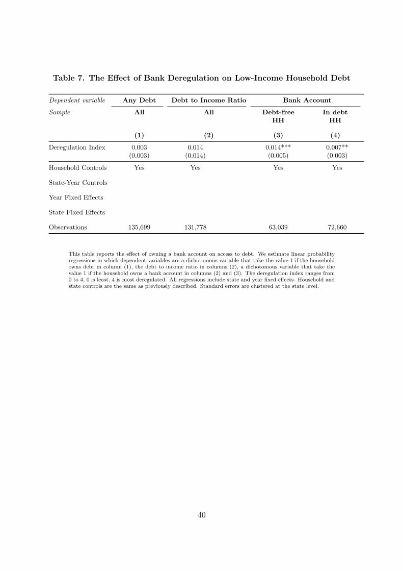
Table 7. The Effect of Bank Deregulation on Low-Income Household Debt

Dependent variable Any Debt Debt to Income Ratio Bank Account

Sample All All Debt-free In debtHH HH

(1) (2) (3) (4)

Deregulation Index 0.003 0.014 0.014*** 0.007**(0.003) (0.014) (0.005) (0.003)

Household Controls Yes Yes Yes Yes

State-Year Controls

Year Fixed Effects

State Fixed Effects

Observations 135,699 131,778 63,039 72,660

This table reports the effect of owning a bank account on access to debt. We estimate linear probabilityregressions in which dependent variables are a dichotomous variable that take the value 1 if the householdowns debt in column (1), the debt to income ratio in columns (2), a dichotomous variable that take thevalue 1 if the household owns a bank account in columns (2) and (3). The deregulation index ranges from0 to 4, 0 is least, 4 is most deregulated. All regressions include state and year fixed effects. Household andstate controls are the same as previously described. Standard errors are clustered at the state level.

40

Table 8. Ruling Out Demand Factors

Dependent variable =1 if the household holds a bank account

Sample All Likely unemployed Not likely unemployed

(1) (2) (3) (4) (5) (6)

Deregulation Index 0.012*** 0.012*** 0.012*** 0.010*** 0.013*** 0.011***(0.004) (0.004) (0.004) (0.004) (0.005) (0.004)

Unemployed HH Head 0.012*** 0.012*** 0.012***(0.004) (0.004) (0.004)

Any HH Member Unemployed 0.017***(0.004)

UE rate - Poor -0.085(0.051)

UE rate - Low Inc. -0.037(0.095)

UE rate - Other -0.056(0.311)

UE rate - Poor & Black 0.015(0.013)

UE rate -Low Income & Black 0.031(0.023)

UE rate - Poor & White -0.143**(0.058)

UE rate - Low Income & Black -0.105(0.106)

UE rate - Other & Black -0.005(0.041)

UE rate - Other & White 0.000(0.345)

Household Controls Yes Yes Yes Yes Yes Yes

State-Year Controls Yes Yes Yes Yes Yes Yes

Year Fixed Effects Yes Yes Yes Yes Yes Yes

State Fixed Effects Yes Yes Yes Yes Yes Yes

Observations 136,176 136,176 136,176 136,176 67,455 68,721

This table reports the effect of Interstate Branching Deregulation Index on the likelihood to have a bankaccount depending on various measure of the unemployment rate in the the state of location. In column(5) and (6), we estimate the probability to be unemployed based on household and state characteristics andsplit the sample between households with a probability below the median sample (column (5)) and abovemedian sample (column (6)). Standard errors are clustered by state.

41

Table 9. Robustness Checks

Dependent Variable =1 if the household holds a bank account

All Periods States

Sample After Before All Only Largest1997 2005 Deregulated

(1) (2) (3) (4) (5) (6) (7)

Deregulation Index 0.011** 0.015*** 0.013*** 0.011** 0.014**(0.005) (0.005) (0.004) (0.005) (0.005)

Placebo Index -0.002(0.004)

Deregulation Dummy 0.020*(0.011)

Household Controls Yes Yes Yes Yes Yes Yes Yes

State-Year Controls Yes Yes Yes Yes Yes Yes Yes

Year Fixed Effects Yes Yes Yes Yes Yes Yes Yes

State Fixed Effects Yes Yes Yes Yes Yes Yes Yes

State × Year Trend - Yes - - - - -

Observations 136,176 136,176 108,116 112,339 136,176 122,005 72,716

This table reports results from linear probability model regressions on access to bank accounts. Columns(1) and (2) and (5) include the whole sample. In columns (3) and (4) data are split into two sub-periods:(1997-2010) and (1993-2006). In column (6) the sample is restricted to states with at least one deregulationover the 1993-2010 period, and in column (7) to the largest 10 states. The dependent variable is 1 ifthe household holds a checking or a savings account (SIPP 1993 - 2010). The explanatory variable is thederegulation index in each column, except in column (1) and in column (5). In column (1) the dependantvariable is a placebo index. In column (5) the dependant variable is a dummy with value 1 if the deregulationindex is strictly higher than 0. All regressions include state and year fixed effects. Column (2) also includesstate*trend effects. Household and state controls include controls for family type, race, age, size of thehousehold, education, receipt of Social Security income or transfer income, monthly income, unemployedstatus and state unemployment, population (log) and unemployment rate. Standard errors are clusteredby state.

42

Appendix A Tables

Table A.1. State Interstate Branching Laws: 1994-2010

This table shows for every state the year in which the deregulation reforms came into effect and gives thederegulation index resulting from these changes. The index ranges from 0 to 4, 4 indicating maximumopenness to out-of-state branching.

State Effective No Allows Allows Deposit IndexYear Minimum Age De Novo Single Branch cap higher

on target Branching Acquisition than 30%Alabama 1997 0 0 0 1 1Alaska 1994 0 0 1 1 2Arizona 1996 0 0 0 1 1Arizona 2001 0 0 1 1 2Arkansas 1997 0 0 0 0 0California 1995 0 0 0 1 1Colorado 1997 0 0 0 0 0Connecticut 1995 0 1 1 1 3Delaware 1995 0 0 0 1 1DC 1996 1 1 1 1 4Florida 1997 0 0 0 1 1Georgia 1997 0 0 0 1 1Georgia 2002 0 0 0 1 1Hawaii 1997 0 0 0 1 1Hawaii 2001 1 1 1 1 4Idaho 1995 0 0 0 1 1Illinois 1997 0 0 0 1 1Illinois 2004 1 1 1 1 4Indiana 1997 1 1 1 1 4Indiana 1998 0 1 1 1 3Iowa 1996 0 0 0 0 0Kansas 1995 0 0 0 0 0Kentucky 1997 0 0 0 0 0Kentucky 2000 1 0 0 0 1Kentucky 2004 1 0 0 0 1Louisiana 1997 0 0 0 1 1Maine 1997 1 1 1 1 4Maryland 1995 1 1 1 1 4Massachussets 1996 1 0 0 1 2Michigan 1995 1 1 1 1 4Minnesota 1997 0 0 0 1 1Mississipi 1997 0 0 0 0 0Missouri 1995 0 0 0 0 0Montana 2001 0 0 0 0 0

43

Table A.2. State Interstate Branching Laws: 1994-2010 (End)

This table shows for every state the year in which the deregulation reforms came into effect and gives thederegulation index resulting from these changes. The index ranges from 0 to 4, 4 indicating maximumopenness to out-of-state branching.

State Effective No Allows Allows Deposit IndexYear Minimum Age De Novo Single Branch cap higher

on target Branching Acquisition than 30%Nebraska 1997 0 0 0 0 0Nevada 1995 0 1 1 1 3New Hampshire 1997 0 0 0 0 0New Hampshire 2000 0 1 1 1 3New Hampshire 2002 1 1 1 1 4New Jersey 1996 1 0 1 1 3New Mexico 1996 1 0 0 0 1News York 1997 0 0 1 1 2North Carolina 1995 1 1 1 1 4North Dakota 1997 1 0 0 0 1North Dakota 2003 1 1 1 0 3Ohio 1997 1 1 1 1 4Oklahoma 1997 0 0 0 0 0Oklahoma 2000 1 1 1 0 3Oregon 1997 0 0 0 0 1Pennsylvania 1995 1 1 1 1 4Rhode Island 1995 1 1 1 1 4South Carolina 1996 0 0 0 1 1South Dakota 1996 0 0 0 1 1Tennessee 1997 0 0 0 1 1Tennessee 1998 0 0 1 1 2Tennessee 2001 0 1 1 1 3Tennessee 2003 0 1 1 1 3Texas 1995 0 1 1 0 2Texas 1995 0 0 0 0 0Texas 1999 1 1 1 0 3Utah 1995 0 0 1 1 2Utah 2001 0 1 1 1 3Vermont 1996 0 0 1 1 2Vermont 2001 0 1 1 1 3Virginia 1995 1 1 1 1 4Washington 1996 0 0 0 0 1Washington 2005 0 1 1 1 3West Virginia 1997 0 1 1 0 2Wisconsin 1996 0 0 0 1 1Wyoming 1997 0 0 0 1 1

44

Table A.3. Percent of Unbanked Households by Data Source and Year

Year Survey of Panel Study SIPPIncome and of Income (low-income

Program Participation Dynamics Households)

1993 16.4 36.3

1994 16.5 22 35.5

1995 16.8 35.6

1996 17.8 36.8

1997 19.2 39.2

1998 19.1 38.6

1999 19.4 23.3 38.8

2000 19.5 38.5

2001 20.1 24.8 38.6

2002 21.4 40.6

2003 22.4 25.7 40.6

2004 19.0 38.6

2005 18.6 25.8 36.7

2009 19.0 26.9 36.7

2010 20.6 38.4

This table reports the share of unbanked households. Percentages are authors’ calculations except for the1994 Panel Study and Income Dynamics one, which is from Hogarth and O’Donnell (1999).

45

Table

A.4

.T

he

Impact

of

Bank

Dere

gula

tion

on

County

Pro

speri

ty

Depen

den

tvariable

Pers

on

al

Incom

eU

nem

plo

ym

ent

Rate

Povert

yR

ate

Hou

seh

old

Levera

ge

Counties

All

Bla

ckP

oor

All

Bla

ckP

oor

All

Bla

ckP

oor

All

Bla

ckP

oor

(1)

(2)

(3)

(4)

(5)

(6)

(7)

(8)

(9)

(10)

(11)

(12)

Der

egu

lati

on0.

001

0.00

50.

012

0.0

00

-0.0

00

-0.0

02

-0.0

00

0.0

02

-0.0

03

-0.0

08

-0.0

05

-0.0

07

(0.0

06)

(0.0

06)

(0.0

07)

(0.0

01)

(0.0

01)

(0.0

02)

(0.0

02)

(0.0

02)

(0.0

03)

(0.0

11)

(0.0

11)

(0.0

23)

Cou

nty

-Yea

rY

esY

esY

esY

esY

esY

esY

esY

esY

esY

esY

esY

es

Yea

rF

EY

esY

esY

esY

esY

esY

esY

esY

esY

esY

esY

esY

es

Cou

nty

FE

Yes

Yes

Yes

Yes

Yes

Yes

Yes

Yes

Yes

Yes

Yes

Yes

Ob

s.59

,742

14,9

2014

,920

59,7

00

14,9

06

14,9

18

59,6

85

14,9

14

14,9

14

27,3

75

8,0

73

6,5

78

Th

ista

ble

rep

ort

slin

ear

pro

bab

ilit

yre

gre

ssio

ns

of

the

Inte

rsta

teB

ran

chin

gD

ereg

ula

tion

Ind

exon

acc

ess

tob

an

kacc

ou

nts

.T

he

dep

end

ent

vari

ab

leeq

uals

1if

the

hou

seh

old

hold

sa

chec

kin

gor

asa

vin

gs

acc

ou

nt

(SIP

P1993

-2010).

Th

ed

ereg

ula

tion

ind

exra

nges

from

0to

4,

0is

least

,4

ism

ost

der

egu

late

d.

Colu

mn

(1)

does

not

incl

ud

eany

contr

ols

wh

erea

sco

lum

ns

(2),

(3)

an

d(4

)in

clu

de

hou

seh

old

contr

ols

,p

lus

state

-yea

rco

ntr

ols

inco

lum

ns

(3)

an

d(4

).A

llre

gre

ssio

ns

incl

ud

est

ate

an

dyea

rfi

xed

effec

ts.

Inco

lum

n(4

)th

ed

ereg

ula

tion

ind

exis

split

into

fou

rsu

b-p

erio

ds:

more

than

3yea

rsb

efore

der

egu

lati

on

,le

ssth

an

3yea

rsb

efore

der

egu

lati

on

,0

to3

yea

rsaft

erd

ereg

ula

tion

,an

dm

ore

than

3yea

rsaft

erd

ereg

ula

tion

,w

her

ed

ereg

ula

tion

corr

esp

on

ds

toth

ere

moval

of

at

least

two

ou

tof

the

fou

rp

oss

ible

rest

rict

ion

s.H

ou

seh

old

an

dst

ate

-yea

rco

ntr

ols

incl

ud

eco

ntr

ols

for

fam

ily

typ

e,ra

ce,

age,

size

of

the

hou

seh

old

,ed

uca

tion

,re

ceip

tof

Soci

al

Sec

uri

tyin

com

eor

tran

sfer

inco

me,

month

lyin

com

ean

dst

ate

un

emp

loym

ent,

pop

ula

tion

(log),

GD

Pgro

wth

an

da

rep

ub

lica

nd

um

my.

Sta

nd

ard

erro

rsare

clu

ster

edby

state

.

46

Table A.5. Standard Determinants of Banked Households

Dependent Variable =1 if the household holds a bank account

Household Controls

Black -0.162*** (0.010)

Married Couple 0.091*** (0.006)

Single Female-Headed 0.035*** (0.006)

Household Size -0.020*** (0.002)

Age 0.004*** (0.000)

Elementary Education 0.091 (0.080)

High School Education 0.193** (0.080)

College Education 0.308*** (0.082)

Monthly Household Income 0.00*** (0.00)

Income < Poverty Threshold -0.059*** (0.005)

Receive Social Security 0.013* (0.007)

Receive transfer income -0.139*** (0.007)

Head unemployed 0.012** (0.004)

State-Year Controls

GDP Growth -0.103 (0.129)

Population -0.037 (0.132)

State Unemployment -0.003 (0.006)

Year Fixed Effects Yes

State Fixed Effects Yes

Observations 136,176

This table reports a linear probability regression of household and state-year controls on access to bankaccounts. The dependent variable equals 1 if the household holds either a checking or savings account(SIPP 1993 - 2010). The regression includes state and year fixed effects. Standard errors are clustered bystate.

47

Table A.6. The Impact of Bank Deregulation on the Share of Banked House-holds: Evidence on Racial Discrimination (2)

Slave Antimisce No Fair Share ofTerritory -genation Housing Law interacial

Law marriage

No Yes No Yes No Yes >Median <Median

(1) (2) (3) (4) (5) (6) (7) (8)

Deregulation Index 0.005 0.009 0.007 0.008 0.002 0.013** 0.008 0.011*(0.006) (0.006) (0.005) (0.007) (0.007) (0.006) (0.005) (0.007)

Index x Black -0.002 0.022*** 0.003 0.022*** -0.005 0.023*** -0.001 0.022***(0.008) (0.005) (0.008) (0.006) (0.007) (0.005) (0.006) (0.006)

Household Controls Yes Yes Yes Yes Yes Yes Yes Yes

State-Year Controls Yes Yes Yes Yes Yes Yes Yes Yes

Year Fixed Effects Yes Yes Yes Yes Yes Yes Yes Yes

State Fixed Effects Yes Yes Yes Yes Yes Yes Yes Yes

Observations 66,017 69,917 76,913 57,805 66,779 69,397 77,960 58,216

This table reports linear probability regressions of the Interstate Branching Deregulation Index on accessto bank accounts and its interaction with a black dummy. The dependent variable equals 1 if the householdholds a checking or savings account (SIPP 1993 - 2010). The deregulation index ranges from 0 to 4, 0is least, 4 is most deregulated. For each set of regressions, the data are split into two mutually exclusivesamples: slave state in the year immediately prior to the Civil War (yes or no), anti-miscegenation lawnot repealed until after the US Supreme Court’s 1967 decision in Loving v.Virginia (yes or no), no fairhousing law until federally mandated by the Fair Housing Act of 1968 (yes or no), racial bias rate, asmeasured by the interracial marriage rate (below or above median). All regressions include state andyear fixed effects. Household and state controls include controls for family type, race, age, size of thehousehold, education, receipt of Social Security income or transfer income, monthly income, unemployedstatus and state unemployment, population (log), GDP growth and a republican dummy. Standard Errorsare clustered by state.

48

Table A.7. Racial Discrimination Across Income Groups

Very Poor Poor Low Income Middle IncomeHH HH HH HH

(1) (2) (3) (4)

Deregulation Index 0.019*** 0.015* 0.012** 0.006(0.007) (0.008) (0.006) (0.004)

Index x Black x Discr. 0.023* 0.029*** 0.030*** 0.023**(0.012) (0.010) (0.011) (0.012)

Household Controls Yes Yes Yes Yes

State-Year Controls Yes Yes Yes Yes

Year Fixed Effects Yes Yes Yes Yes

State Fixed Effects Yes Yes Yes Yes

Observations 18,069 34,401 83,706 48,343

This table reports linear probability regressions of the Interstate Branching Deregulation Index on accessto bank accounts and its interaction with a black dummy. The dependent variable equals 1 if the householdholds a checking or savings account (SIPP 1993 - 2010). The deregulation index ranges from 0 to 4, 0is least, 4 is most deregulated. Data are split into four exclusive samples of households based on theirannual income: very poor (below half the poverty line), poor (between half and once the poverty line),low-income (between once and twice the poverty line) and middle income households (between twice andthree times the poverty line). In column (1) we estimate linear probability regressions of the InterstateBranching Deregulation Index on access to banking and its interaction with a poor household (includingvery poor households) dummy and with a low-income household dummy. Regressions also include blackx discrimination, index x deregulation, black*deregulation controls. Household and State controls includecontrols for family type, race, age, size of the household, education, receipt of Social Security incomeor transfer income, monthly income, unemployed status and state unemployment, population (log) andunemployment rate. Standard Errors are clustered by state.

49

Table A.8. Addressing Endogeneity Concerns

Duration Model for the Time until Deregulation

(1) (2) (3) (4) (5) (6)

Unbanked HH (%) -1.85 -4.14(1.916) (3.033)

Unbanked Low income HH (%)) -3.98(2.778)

Unbanked Black HH (%) 0.38(3.524)

Black HH (%) -0.26 2.64(1.496) (2.380)

UE rate (%) 0.12 0.21(0.121) (0.186)

GDP per capita 0.03** 0.01(0.014) (0.019)

Republican dummy -0.18 0.22(0.372) (0.439)

Share of small banks -19.57*** -18.97***(5.134) (6.172)

Relative capital ratio of small banks 0.00 0.00(0.000) (0.000)

Relative size of insurance 1.01*** 1.17***(0.369) (0.323)

Observations 1,773 1,773 1,773 1,773 1,773 1,773

The hazard model is Weibull, where the dependent variable is the log expected time to deregulation.All variables are measured for each state in each year. The share of unbanked households, low-incomeunbanked households or black unbanked households are measured at the state level in 1994. The shareof black people in the state population, unemployment rate and real GDP per capita is at the state-yearlevel. Share of small banks is the percent of banking assets in the state held by banks below the mediansize of banks in each state in each year. Relative capital ratio of small banks is the capital to assets ratioof small banks minus that of large banks. Relative size of insurance relative to banking plus insurance inthe state is measured as gross state product from insurance divided by gross state product from insuranceplus banking. Republican is equal to one if the majority of the voters chose the Republican candidate inthe latest presidential election.

50

Table A.9. Deregulation and Branch Density: Alternative Proxies of Discrim-ination

Dependent variable Branch Density

Proxy Discrimination Antimiscegenation Law No Fair Housing Interracial MarriageDiscrimination Discrimination Discrimination

No Yes No Yes No Yes

Deregulation 0.073** 0.180*** 0.012*** 0.089*** 0.078** 0.128**(0.030) (0.043) (0.004) (0.032) (0.031) (0.056)

County-Year Yes Yes Yes Yes Yes Yes

Year FE Yes Yes Yes Yes Yes Yes

County FE Yes Yes Yes Yes Yes Yes

Obs. 5,032 6,692 4,154 7,602 5,095 6,661

51

Appendix B Variables Definitions

State-level variables

State GDP Growth: annual growth rate in gross state product (GSP) using data obtainedfrom the U.S. Bureau of Economic Analysis Region Tables.

Population: log of total state population from the U.S. Bureau of Economic AnalysisRegion Tables.

State Unemployment: the state unemployment rate, obtained from the U.S. Bureau ofLabor Statistics.

CPS Data

To construct unemployment rate by racial and income categories, we use publicly-availablemicrodata from IPUMS-CPS (Ruggles et al. 2010) for the years 1994 to 2010. We selectthe sample as follow. We drop the population not in the labor force (labforce = 13) andin military (empstat=13) and keep persons between the age of 16 and 64. We identifyfamilies below the poverty line if their total family income ftotval is below the thresholdgiven by the CPS (variable cutoff). Finally, we collapse the data at the state-year levelusing population weight wtsupp.

52