Bank behavior based on internal credit ratings of … behavior based on internal credit ratings of...

CFS Working Paper No. 98/08

Bank behavior based on internal

credit ratings of borrowers*

Achim Machauer, Martin Weber**

March 20, 1998

Abstract: This study examines the relation of bank loan terms like interest rates, collateral,

and lines of credit to borrower risk defined by the banks’ internal credit rating. The analysis

is not restricted to a static view. It also incorporates rating transition and its implications on

the relation. Money illusion and phenomena linked with relationship banking are discovered

as important factors. The results show that riskier borrowers pay higher loan rate premiums

and rely more on bank finance. Housebanks obtain more collateral and provide more

finance. Caused by money illusion in times of high market interest rates loan rate premiums

are relatively small whereas in times of low market interest rates they are relatively high.

There was no evidence for an appropriate adjustment of loan terms to rating changes. But

bank market power represented by a weighted average of credit rating before and after a

rating transition serves to compensate for low earlier profits caused by phenomena of

interest rate smoothing.

Keywords: Bank loan terms; Internal borrower rating; Relationship banking; Money Illusion

JEL classification: G 21

Fields: banking

* This paper is the result of a research project on Credit Management at the Center for Financial Studies,

Frankfurt. See also the acknowledgements at the end of the text.** Lehrstuhl für Allgemeine Betriebswirtschaftslehre und Finanzwirtschaft, insbesondere

Bankbetriebslehre, Universität Mannheim, L 5,2, 68131 Mannheim, Germany, Email:

[email protected], [email protected].

-1-

1. Introduction

In credit risk management a usual goal is to price loans according to their risk exposure.1

The purpose of this tactic is obvious. Lenders should be compensated for the risk that

borrowers do not repay their loans. Additionally, if loans are priced according to the

involved risk, modern approaches of bank controlling allow a profound management of

bank capital. Thus the question arises whether or not risk-adjusted loan pricing really exists

as a phenomenon. A contradictory explanation could be that cross-selling cause banks to

provide cheap loans in order to attract customers for other profitable business. Volume

oriented wages might induce bank employees to increase volume by undertaking business

with borrowers of bad quality. Another factor might be the phenomena of interest rate

smoothing during a bank-borrower relationship. Petersen and Rajan (1995) and Fried and

Howitt (1980) have shown that smoothing of interest rates in relation to borrower risk and

in relation to market interest rates enhance welfare. Furthermore, Money illusion is a

phenomenon of interest rate smoothing which relies more on a bias of the borrowers’

evaluation of loan rates.

In this paper, we study the relation between terms of lending and borrower risk with

respect to the opposing phenomena mentioned above. Furthermore we are interested in the

adaptation of terms of lending by banks when borrower risk changes over time. The

questions that arise are:

(1) is there a relation between terms of lending and borrower risk and which

factors oppose such a relation,

(2) does this relation hold or deteriorate when borrower ratings change ?

Our analysis is based on data from five leading German banks. We obtained randomly

chosen credit files of two hundred small and medium-sized firms from the years 1992 to

1996. Using regression analysis we identify factors which explain

- interest rate premiums firms have to pay

- the amount of collateral relative to the firms’ overall credit line

- the credit line relative to their balance-sheet total and

- the changes of interest rate premiums from one credit analysis of the bank to the

next.

1 See e.g. Saunders (1997), p. 583.

-2-

Following Berger and Udell (1995) and Blackwell and Winters (1997), we restrict our

analysis of interest rate premiums to current accounts. This kind of loan is relationship

driven and its short-term character allows us to compare interest rates easily. The analyses

of collateral and lines of credit refer to the bank-borrower relationship as a whole. We

consider small and medium-sized firms because these firms usually do not use capital

markets as an alternative source of finance.

Our results show that riskier borrowers pay higher loan rate premiums and rely more on

bank loans. There is no significant relation between collateralization and borrower risk. We

found strong effects of money illusion with relatively small loan rate premiums in times of

high market interest rates and relatively high ones in times of low market interest rates.

Housebank relationships have no influence on premiums but banks within such a

relationship obtain more collateral in relation to the borrowers credit line and provide more

finance relative to the balance-sheet total of the borrower. The analysis of rating changes

over time provides no evidence for an appropriate adjustment of loan terms.

The remainder of this paper is organized in the following manner. In Section 2 we

discuss in detail arguments for and against a relation of loan terms and borrower risk. Then,

in Section 3, we describe the relevant data set. In Section 4 we analyze the relation of loan

rates, collateralization and lines of credit to borrower risk and other important factors. The

adaptation of these terms of lending (bank behavior) on changes of borrower risk (rating

transition) is studied in Section 5. In Section 6 we discuss implications of the results and

make suggestions for future research.

2. Recent literature

2.1. Loan pricing and borrower risk

Loan pricing according to risk exposure serves to compensate lenders for the risk that

borrowers do not repay. Cross-selling provides an obvious explanation of the phenomenon

that loan prices do not reflect credit risk accordingly. In negotiating terms of lending, banks

often make concessions because they are involved in other profitable business with the

customer. In this case the entire yield of the customer relationship must be taken into

account. However, this poses a difficulty due to the unavailability of data.

Besides this intuitive argument on the missing link between loan interest rates and

borrower risk there are models in banking theory, especially on debt renegotiation, that

come to the conclusion that no monotonous relation between loan rates and credit risk

-3-

should be expected. Gorton and Kahn (1996), for example, show that it is rational for the

bank to lower loan rates for special classes of bad borrowers during the credit period in

order to give them the incentive not to add risk inefficiently.

There is not much empirical evidence on the relation of loan interest rates and borrower

risk. Blackwell and Winters (1997) use a rather rough classification of medium risk and low

risk borrowers2 which they deduced from the monitoring frequency of the lending banks.

They found significant higher loan rate premiums for medium risk borrowers than for low

risk borrowers.

2.2. Loan pricing and relationship banking

The literature on relationship banking contributes opposing theoretical arguments and

empirical results which can be employed to explain why terms of lending should not be risk-

adjusted. All arguments depend more or less on the possibility of the bank to bind their

customers, that is to commit them implicitly to future business with the bank. In this context

banks can smooth interest rates over time in response to changes of borrower risk or in

response to changes of market interest rates (see Berlin and Mester (1997)). The aim is to

enhance welfare which can be shared between the two contracting parties. In section 2.6 we

will discuss research showing that inefficient credit rationing can be overcome by such

smoothing behavior.3

A binding relationship is obviously achieved in a monopoly situation, e.g. when the bank

is the only financier of borrowers in a certain region. Another way of achieving a binding

relationship is to build up an information advantage during a relationship which enables the

bank to assess borrower risk more accurately than competing banks and thus to offer lower

loan prices to low risk companies than any other competitor (see Fischer (1990), Sharpe

(1990) and Greenbaum, Kanatas and Venezia (1989)). Since the assessment of competitors

more often deviates from the exact borrower risk, these competitors must require higher

loan rates to compensate for a possible bad borrower selection. Thus in this relationship the

bank has considerable leeway to compensate for lower interest rates accrued in earlier

stages of the relationship.

Theoretical conclusions on relationship banking are worthless if a relationship does not

exist. Mayer (1988) attributes close relationships between bank and customers to Japan and

2 Blackwell and Winters do not have a category of high risk borrowers in their study.3 See the passage on credit lines below.

-4-

Germany.4 However, Edwards and Fischer (1994) and Fischer (1990) concluded that this is

not true for Germany. In the case of Japan, Hoshi, Kashyab and Scharfstein (1990, 1991)

provide empirical evidence for the existence of lively main bank relationships especially in

firm conglomerates called keiretsu. Based on our results below we can state that so called

housebank relationships exist and have influence on the banks’ decision making.

2.3. Loan rate smoothing in response to changes of borrower risk

Assuming binding relationships between borrowers and lenders, Petersen and Rajan

(1995) show positive effects of interest rate smoothing in response to credit risk changes.

At the beginning of the relationship, as in Stiglitz and Weiss (1981), there is no possibility to

select borrowers according to their quality. Hence, problems of adverse selection and moral

hazard have to be considered. These problems can be solved by charging low interest rates

at the beginning. In later stages of the relationship, borrower selection problems are

resolved by having monitored former successful projects of surviving borrowers. With these

borrowers high interest rates can be achieved. These high interest interest rates are still low

compared to interest rate offers of competing banks with no earlier relationship to these

customers. These competing banks have to rely on an assessment of the average default

probability of possible new borrowers, which is higher because no pre-selection of borrower

quality has taken place.

Similar smoothing effects can be found when banks offer cheap loans to customers in

times of financial distress or in times of big investment efforts in expectation of future

compensation. The underlying presumption is again that borrowers can be committed to

stay in relation with the bank and thus give it the possibility to make profitable business later

when they are of a better quality.

Petersen and Rajan (1994) provide empirical evidence on the effects of bank-borrower

relationships on loan pricing for small firms in the United States. Their results suggest no

significant influence. Contrarily, Berger and Udell (1995) who analyzed the same data set

obtained significant results. They discovered that small firms with longer banking

relationships borrow at lower rates.

2.4. Loan rate smoothing in response to market rate changes and money illusion

Interest rate insurance is a second phenomenon of interest rate smoothing. It is caused by

the response of the contracting parties to changes in market interest rates, and is based on

4 See Mayer (1988), p. 1180.

-5-

the desire of risk averse borrowers to insure against interest rate risk. On average they

would pay higher loan rates if the bank was willing to keep the rates less variable than

capital market interest rates. Fried and Howitt (1980) model this possibility of risk sharing.

Money illusion on the part of the borrowers is another phenomenon which causes

interest rate smoothing in response to changes in market interest rates over time. In contrast

to interest rate insurance it does not assume a binding relationship. Money illusion is a bias

in the assessment of the real value of economic transactions, induced by a nominal

evaluation.5 In the context of firms that evaluate bank loans it is expected that, in times of

high capital market interest rates, offered loan rates seem too high to them. These firms do

not consider the banks’ profit margins, i.e. the nominal loan rate less the prime rate – what

they should do. As a consequence, in times of high capital market rates banks realize smaller

profit margins compared to times of low capital market rates. In times of low market rates

they require higher margins. In contrast to interest rate insurance which depends on

personal risk aversion we see money illusion in this context as an overall bias in decision

making of borrowers. Thus it is not necessary for the bank to bind single customers for

profit compensation. If this bias really exists even new borrowers will accept higher

premiums in times of low market rates as a result of their orientation on nominal values.

Berger and Udell (1992) were the first who conducted a study on loan rate smoothing or

loan rate stickiness in response to changes in market interest rates using individual loan

data. In contrast to earlier studies which relied on macroeconomic data they suggest that

most of the stickiness does not reflect rationing which would be consistent with the model

of Petersen and Rajan (1995). They also suggest that interest rate insurance is achieved

through fixed-rate agreements rather than through floating-rate agreements. As we study

floating-rate agreements, money illusion should be a more important factor for interest rate

smoothing.

2.5. Collateral

So far we have only considered loan rates. The following analysis includes collateral and

lines of credit as well. Intuitively one would think that riskier borrowers have to provide

more collateral and obtain less credit because banks try to reduce their exposure to such

borrowers. On the other hand good borrowers are more likely to pledge collateral because

5 Shafir, Diamond and Tversky (1997) review experimental studies concerning money illusion. See also

Fisher (1928) for an early discussion.

-6-

in general they should have more assets available. This second view is supported by Bester

(1985) and Besanko and Thakor (1987) in their models of borrower selection at the

beginning of a bank-borrower relationship. Additionally, Boot and Thakor (1994)

demonstrate that the duration of a bank-borrower relationship has effects on collateral as

well as on interest rates. They show that borrowers have to pay high interest rates and

pledge collateral in early stages of the relationship, whereas they get lower rates and do not

need to pledge collateral later on, when successful projects and thus good borrowers are

identified.

The empirical literature on the relation of collateral and borrower risk is not very broad.

In an early study Berger and Udell (1990) found that high risk borrowers pledge more

collateral but nevertheless their credits stay riskier than those of low risk borrowers.

However, these results seem problematic because their proxy of borrower risk, loan rate

minus prime rate, is a rather rough indicator. The results of Berger and Udell (1995)

suggest that older firms with greater experience and longer banking relationships pledge

collateral less often.

2.6. Credit lines

Stiglitz and Weiss (1981) explain restrictive lending policies of banks as a consequence

of asymmetric information on borrower quality. Models as of Bester (1985) and Besanko

and Thakor (1987) solve this problem by introducing collateral as a sorting device to

identify borrower quality. Petersen and Rajan (1995,1994) show theoretically and

empirically that another key to overcoming this phenomenon is the possibility of learning

about borrower quality through time. As a consequence borrowers with a strong bank-

borrower relationship receive more credit on average. This conclusion is sustained by

evidence from Japan provided by Hoshi, Kashyab and Scharfstein (1990, 1991).

3. Data

Our data on bank-borrower relationships was drawn from a set of credit files coming

from five major German banks: Bayerische Vereinbsbank, Deutsche Bank, DG Bank,

Dresdner Bank, and WestLB.6 The data covers the period from January 1992 to December

1996. Since the analysis focusses on small and medium-sized firms the set of feasible

relationships is limited to firms with an annual turnover between DM 50 and 500 million.

6 These banks represent five of the nine biggest banks in Germany at the end of the year 1996.

-7-

Furthermore the minimum loan size should not be under DM 3 million.7 No relationships

with firms of the eastern part of Germany, the former German Democratic Republic, were

involved because the nature of such relationships is dominated by industrial restructuring

with a specific risk structure in credit portfolios that is expected to differ substantially from

that of customers in the western part of Germany.8

The data consists of two samples. Sample A has 125 customer relationships, 25 of each

bank, taken randomly from the population of ”all” the borrowers described above. Usually

the whole credit history of these relationships is available for the period of 1992 to 1996.

The second sample, called Sample P, was drawn from a subset of the population of all

borrowers described above, with the special characteristic that they are ”problematic” or

"potentially distressed". Of each bank 15 customers are part of this sample, i.e. 75

altogether. The characteristic ”problematic” or ”potentially distressed” was defined as a

borrower being of category 5 or 6 on a calibrated credit rating scale of 1 to 6 (described

below) once between 1992 and 1996. Sample P was drawn to strengthen the number of

customers with poor credit ratings which otherwise would be too small to generate

statistically significant results.

The rating scale from 1 to 6 was created by Elsas, Henke, Machauer, Rott and Schenk

(1997) to make the internal ratings of the five banks in this study comparable. In order to

achieve this calibration the rating subcategories on certain borrower characteristics were

matched to get the new six rating classes with 1 being very good, 2 being good or above

average, 3 being average, 4 being below average, 5 being problematic and 6 being very

much in danger of default.

4. Terms of lending and borrower risk

In the following, terms of lending (interest rates, collateral and lines of credit) are

studied separately with respect to their relation to borrower risk. We do not look at

covenants because, in Germany, they are typically standardized with no variations according

to borrower risk, especially in small firm finance. For each of the three terms of lending we

give an impression of the relation to borrower risk via a boxplot and then present results of

a regression analysis. But first, we want to describe the variables that were used.

7 The exchange rate of the Deutschmark in US-Dollars at the end of 1996 was: .64 DM/US$.8 For a detailed description of the data set see Elsas, Henke, Machauer, Rott and Schenk (1997).

-8-

4.1. Variables

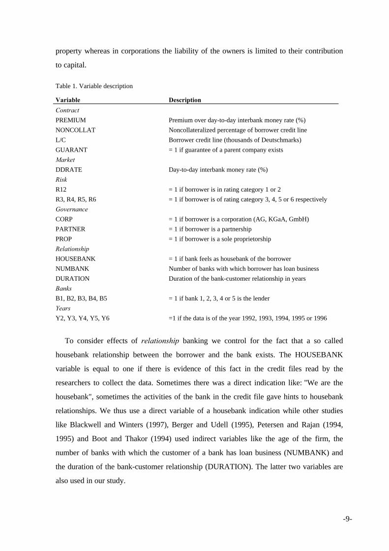
The variables used for this analysis are shown in Table 1. Some of them are also involved

in the analysis of bank behavior on rating transition (Section 5).

We begin by explaining variables of the debt contract. The loan premium (PREM) is

defined as the difference between the loan interest rate for withdrawals on current accounts

and the capital market interest rate for the same duration of lending. We used the interbank

rate for day-to-day money (DDRATE) as our reference because we consider it as the

appropriate market rate for banks to refinance this kind of lending. The premiums on

current account lending or more exactly the underlying nominal interest rates can be

adjusted permanently.

To define the noncollateralized percentage of the lines of credit (NONCOLLAT), we

used the internal evaluation of the liquidation value on which banks base their decision

making. Lines of credit (L/C) include all forms of credit that a bank grants to its customer,

i.e. lines of credit for cash loans, discounted bills, guarantees and margins of derivatives.

They were measured in thousands of deutschmarks (TDM). Banks consider these overall

lines when making decisions about an increase or decrease of their loan business with the

customer.

The variable GUARANT was added to the class of contractual variables. It is a dummy

variable that equals one if the borrower’s liabilities are backed by a guarantee of a parent

company and zero otherwise. In a contract such a clause should very much serve to reduce

credit risk for the bank.

Variables on risk characterize borrower risk, i.e. default risk of borrowers, without

taking collateral into account. Thus dummy variable R12 equals one if a borrower is of

rating category 1 or 2 and zero otherwise. R3 is one if a borrower is of rating category 3

and so on. We combined rating categories 1 and 2 into one variable because only a few

borrowers in our sample were of rating category 1.

Variables on governance characterize the legal form of the firms. The dummy variable

CORP indicates whether the firm is a corporation, i.e. Aktiengesellschaft, Kommandit-

gesellschaft auf Aktien or a Gesellschaft mit beschränkter Haftung in Germany. PARTNER

indicates whether the firm is a partnership like Offene Handelsgesellschaft or

Kommanditgesellschaft and PROP indicates whether there is a sole proprietor of the firm

who usually manages its business like an Einzelunternehmung in Germany. In partnerships

and in proprietorships the owners are liable for the firm’s debt with their whole private

-9-

property whereas in corporations the liability of the owners is limited to their contribution

to capital.

Table 1. Variable description

Variable Description

Contract

PREMIUM Premium over day-to-day interbank money rate (%)

NONCOLLAT Noncollateralized percentage of borrower credit line

L/C Borrower credit line (thousands of Deutschmarks)

GUARANT = 1 if guarantee of a parent company exists

Market

DDRATE Day-to-day interbank money rate (%)

Risk

R12 = 1 if borrower is in rating category 1 or 2

R3, R4, R5, R6 = 1 if borrower is of rating category 3, 4, 5 or 6 respectively

Governance

CORP = 1 if borrower is a corporation (AG, KGaA, GmbH)

PARTNER = 1 if borrower is a partnership

PROP = 1 if borrower is a sole proprietorship

Relationship

HOUSEBANK = 1 if bank feels as housebank of the borrower

NUMBANK Number of banks with which borrower has loan business

DURATION Duration of the bank-customer relationship in years

Banks

B1, B2, B3, B4, B5 = 1 if bank 1, 2, 3, 4 or 5 is the lender

Years

Y2, Y3, Y4, Y5, Y6 =1 if the data is of the year 1992, 1993, 1994, 1995 or 1996

To consider effects of relationship banking we control for the fact that a so called

housebank relationship between the borrower and the bank exists. The HOUSEBANK

variable is equal to one if there is evidence of this fact in the credit files read by the

researchers to collect the data. Sometimes there was a direct indication like: "We are the

housebank", sometimes the activities of the bank in the credit file gave hints to housebank

relationships. We thus use a direct variable of a housebank indication while other studies

like Blackwell and Winters (1997), Berger and Udell (1995), Petersen and Rajan (1994,

1995) and Boot and Thakor (1994) used indirect variables like the age of the firm, the

number of banks with which the customer of a bank has loan business (NUMBANK) and

the duration of the bank-customer relationship (DURATION). The latter two variables are

also used in our study.

-10-

The dummy variables on banks help to control for bank specific effects. B1 to B5 are

equal to one when the credit file which was analyzed came from the related bank. We use

B1 to B5 instead of the banks’ names in order to maintain confidentiality.

Y2 to Y6 are control variables for the years 1992 to 1996. As mentioned above we have

credit file data of borrowers in this period. Each monitoring process was recorded.

Sometimes we had more than one monitoring process per year and sometimes we had only

one in two years time. But generally we have one monitoring process per year.

4.2. Interest rate premiums

Loan interest rate premiums as defined here are rather rough indicators for bank profits

on loans. To get net profits out of it, one has to additionally adjust for other cost

components like fees, administration costs and, most importantly, expected default losses.

The latter component was the variable focussed upon by the analysis in this study. As far as

administration costs and fees are concerned, we assume that they do not vary too much

within a bank over the observed period and likewise between different banks. We cannot

control for these components of the interest rate premium, as there was no (reliable) data

available on that aspect.

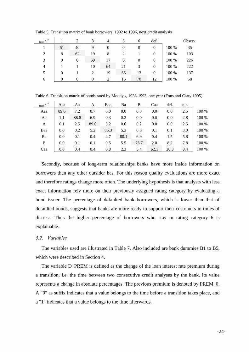
Descriptive analysis

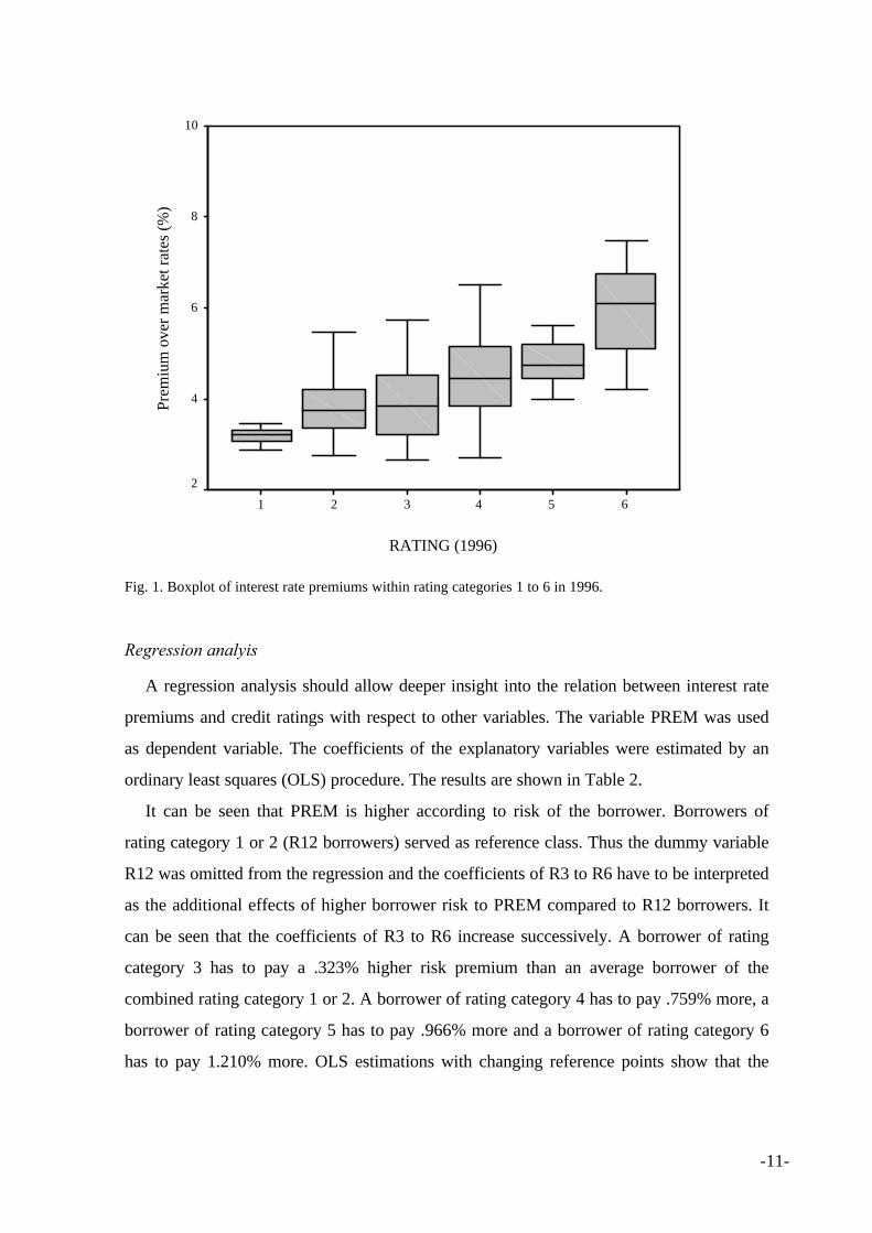
Figure 1 illustrates the distributions of interest rate premiums within each of the six

rating categories in 1996. For this purpose sample A and P were combined to have more

observations in rating categories 5 and 6.

The boxplot indicates that the medians of interest rate premiums are higher when

borrowers are of worse quality. In Figure 1 these medians are represented by the lines

within the boxes. These boxes contain fifty percent of the distribution of premiums. The

bottom line of a box indicates a 25 percentile and the top line indicates a 75 percentile. To

give a more exact impression, the whiskers which lie above the top line of the box and

below the bottom line indicate the 90 and the 10 percentile according to assumptions of

normally distributed premiums.

-11-

RATING (1996)

654321

Prem

ium

ove

r m

arke

t rat

es (

%)

10

8

6

4

2

Fig. 1. Boxplot of interest rate premiums within rating categories 1 to 6 in 1996.

Regression analyis

A regression analysis should allow deeper insight into the relation between interest rate

premiums and credit ratings with respect to other variables. The variable PREM was used

as dependent variable. The coefficients of the explanatory variables were estimated by an

ordinary least squares (OLS) procedure. The results are shown in Table 2.

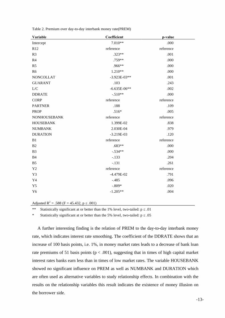
It can be seen that PREM is higher according to risk of the borrower. Borrowers of

rating category 1 or 2 (R12 borrowers) served as reference class. Thus the dummy variable

R12 was omitted from the regression and the coefficients of R3 to R6 have to be interpreted

as the additional effects of higher borrower risk to PREM compared to R12 borrowers. It

can be seen that the coefficients of R3 to R6 increase successively. A borrower of rating

category 3 has to pay a .323% higher risk premium than an average borrower of the

combined rating category 1 or 2. A borrower of rating category 4 has to pay .759% more, a

borrower of rating category 5 has to pay .966% more and a borrower of rating category 6

has to pay 1.210% more. OLS estimations with changing reference points show that the

-12-

differences between neighboring risk classes are significant.9 For these differences we have:

R12 better than R3 (p = .001), R3 better than R4 (p < 001), R4 better than R5 (p = .065).

R5 and R6 do not differ much, the p-value equals .168. But the difference between R4 and

R6 is again significant (p = .008). Thus, we found that there is evidence for a monotonous

relation between borrower quality and interest rate premiums that is statistically and

economically significant.

9 p-values in brackets indicate the significance level.

-13-

Table 2. Premium over day-to-day interbank money rate(PREM)

Variable Coefficient p-value

Intercept 7.010** .000

R12 reference reference

R3 .323** .001

R4 .759** .000

R5 .966** .000

R6 1.210** .000

NONCOLLAT -3.923E-03** .001

GUARANT .103 .243

L/C -6.635E-06** .002

DDRATE -.510** .000

CORP reference reference

PARTNER .188 .109

PROP .516* .005

NONHOUSEBANK reference reference

HOUSEBANK 1.399E-02 .838

NUMBANK 2.030E-04 .979

DURATION -3.219E-03 .120

B1 reference reference

B2 .683** .000

B3 -.534** .000

B4 -.133 .204

B5 -.131 .261

Y2 reference reference

Y3 -4.479E-02 .791

Y4 -.485 .096

Y5 -.809* .020

Y6 -1.205** .004

Adjusted R2 = .588 (F = 45.432, p ≤ .001)

** Statistically significant at or better than the 1% level, two-tailed: p ≤ .01

* Statistically significant at or better than the 5% level, two-tailed: p ≤ .05

A further interesting finding is the relation of PREM to the day-to-day interbank money

rate, which indicates interest rate smoothing. The coefficient of the DDRATE shows that an

increase of 100 basis points, i.e. 1%, in money market rates leads to a decrease of bank loan

rate premiums of 51 basis points (p < .001), suggesting that in times of high capital market

interest rates banks earn less than in times of low market rates. The variable HOUSEBANK

showed no significant influence on PREM as well as NUMBANK and DURATION which

are often used as alternative variables to study relationship effects. In combination with the

results on the relationship variables this result indicates the existence of money illusion on

the borrower side.

-14-

Petersen and Rajan (1994) and Blackwell and Winters (1997) (unlike us) did find

statistically significant influence of NUMBANK and DURATION on PREM but they did

not find any economically significant influence either. Only Berger and Udell (1995) who,

unlike Petersen and Rajan, restricted their analysis to lines of credit found some evidence of

the influence of DURATION on PREM. But all these studies did not use a HOUSEBANK

variable which contains the evaluation of the relationship by the bank. Only Elsas and

Krahnen (1998), who used the same data set as ours, included a HOUSEBANK variable in

their analysis and obtained results similar to ours.

Collateral is a biasing factor in the relation between borrower risk and loan premiums. Of

course risk-adjustment is needless if there is enough collateral involved because only the

unsecured part of a loan is exposed to borrower risk. In our study we could not assign the

appropriate loan interest rate to a specific amount of money exposed to risk because the

different types of loans that sum up to the overall line of credit have interest rates of a

different nature. We therefore did separate analyses of the relation of interest rate

premiums, collateral and lines of credit to borrower risk, and included the rest of the terms

of lending as exogenous variables. In the analysis of PREM the coefficient of

NONCOLLAT, the unsecured percentage of the lines of credit, was statistically significant

(p = .001) suggesting that there is a positive relation between interest rates and collateral.

This finding is in accord with Berger and Udell (1990) and Blackwell and Winters (1997).

However, an additional collateralization of another ten percent of the borrower’s line of

credit only induces an increase of the premium of 3 basis points, i.e. .03 percent, which is

not economically significant. A guarantee of a superior part of the group of firms to which

the borrower belongs to (GUARANT) has no statistically significant effect at all on PREM.

Contrarily, the size of the line of credit is significant at better than the 1% level. A borrower

with a credit line (L/C) that is 10 million DM higher has to pay nearly seven basis points less

of interest. Thus the recognition here is that the larger borrowers pay less. The coefficient

of PROP, which is also significant at better than the 1% level, sustains this conclusion.

Proprietorships which are usually smaller than corporations pay 51.6 basis points more on

average than these. Similar results were found by Berger and Udell (1995).

Special effects due to the belonging of credit files to certain banks are considered by

control variables B1 to B5. It can be seen that Bank No. 2 achieves significantly higher

premiums than the reference Bank No. 1. The average difference is 68.3 basis points which

is significant from an economic point of view. Bank No. 3 has significantly lower margins,

-15-

with a negative coefficient of 53.4 basis points of interest. Banks No. 4 and No. 5 are not

significantly different from Bank No. 1. In reviewing these figures, it is apparent that the

managers of bank No. 2 would agree they were the most successful.

Variables Y2 to Y6 were put into the regression model to control for the effects of time.

The reference point was 1992. As time proceeds to 1996 the effect on PREM becomes

more and more significant. In 1994 there is a negative coefficient of 48.5 basis points

compared to 1992 (p =.096). In 1995 the difference widens to -80.9 basis points (p = .02)

and in 1996 the difference becomes even more obvious with -120.5 basis points (p = .004).

The reason for decreasing margins over time can be explained by increasing competition

between banks as it takes place in Germany and in Europe as a whole. Due to the decrease

in day-to-day money rates from 1992 to 1996, from a level of nearly 10% to a level of about

3%, there is a money illusion effect indicated by the coefficient on DDRATE which

increases premiums from 1992 to 1996. In this respect, the time or competition effect

discovered here is an opposing effect. A link between DDRATE and Y2 to Y6 was detected

by an analysis of multicollinearity. However, another regression of PREM leaving out Y3 to

Y6 shows that the coefficients of the other variables remain robust. Hence we see no biasing

correlation between DDRATE and Y2 to Y6 here.

Further analysis concerning the assumptions necessary to use OLS-estimations like

homoscedasticity, no autocorrelation and normality of residuals showed no significant

opposition to the defined regression model. The adjusted R2 is equal to .588, supporting the

explanatory power of the model (F-value = 45.432 with a p-value below the .001 level).

4.3. Collateral

The unsecured percentage of the credit line in this study refers to the whole loan business

of the borrower with the bank. Since the credit decision of the bank refers to the whole

credit line it would not have made sense to restrict the analysis to the credit line for the

current account.

Descriptive analysis

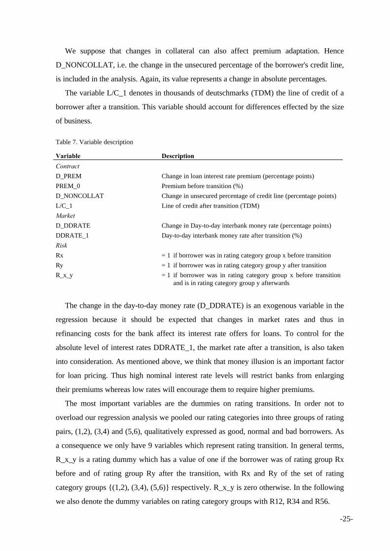
Our goal is to make statements about the relation of terms of lending and risk, especially

borrower risk. Figure 2 illustrates the distributions of the unsecured part of the credit lines

of borrowers within each of the six rating categories. As can be seen, the medians lie around

and above the 60 percent level. The average collateralized percentage of all borrowers in

sample A is 68.6%, with 8.8% of the borrowers fully collateralized and 33.8% not

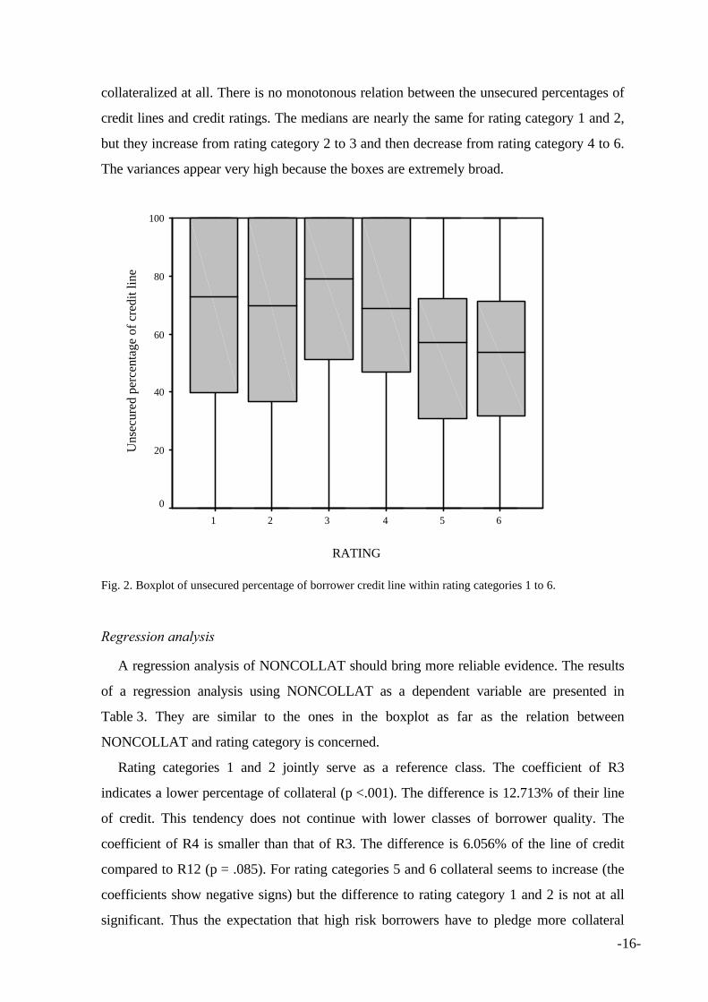
-16-

collateralized at all. There is no monotonous relation between the unsecured percentages of

credit lines and credit ratings. The medians are nearly the same for rating category 1 and 2,

but they increase from rating category 2 to 3 and then decrease from rating category 4 to 6.

The variances appear very high because the boxes are extremely broad.

RATING

654321

Uns

ecur

ed p

erce

ntag

e of

cre

dit l

ine

100

80

60

40

20

0

Fig. 2. Boxplot of unsecured percentage of borrower credit line within rating categories 1 to 6.

Regression analysis

A regression analysis of NONCOLLAT should bring more reliable evidence. The results

of a regression analysis using NONCOLLAT as a dependent variable are presented in

Table 3. They are similar to the ones in the boxplot as far as the relation between

NONCOLLAT and rating category is concerned.

Rating categories 1 and 2 jointly serve as a reference class. The coefficient of R3

indicates a lower percentage of collateral (p <.001). The difference is 12.713% of their line

of credit. This tendency does not continue with lower classes of borrower quality. The

coefficient of R4 is smaller than that of R3. The difference is 6.056% of the line of credit

compared to R12 (p = .085). For rating categories 5 and 6 collateral seems to increase (the

coefficients show negative signs) but the difference to rating category 1 and 2 is not at all

significant. Thus the expectation that high risk borrowers have to pledge more collateral

-17-

than low risk borrowers is not supported throughout the rating categories. Rather, the

opposite is suggested which is in line with Besanko and Thakor (1987). They model that

low risk borrowers tend to offer more collateral and low loan rates instead of less collateral

and high loan rates because their probability of loosing collateral in a default is lower. An

opposite opinion on the relation between collateral and borrower risk could be that good

borrowers, such as those in rating category 1 and 2, need not pledge collateral either

because banks do not require it or the negotiation power of these borrowers is strong.

Contrarily, worse borrowers would have to pledge relatively more collateral at least in order

to reach better loan interest rates if not to get credit at all. The problem of distressed

borrowers is that they can not offer more collateral. On the other side, banks can not reduce

lines of credit without risking that these borrowers go bankrupt. However these

considerations are not at all supported by the regression results.

The coefficient of PREM (-4.817) indicates that collateral and interest rates are not

substitutes (p = .001). But, in accordance with the results of Section 4.2 the coefficient of

PREM in the regression of NONCOLLAT is too small indicating that a borrower must pay

1% more of interest to avoid collateral requirements of 4.817% of his credit line.

A guarantee from the parent company seems to have more influence on the borrower’s

provision of collateral, but in a surprising manner. The coefficient of the variable

GUARANT suggests that such a borrower provides additional collateral which amounts

10.568% of his credit line (p = .001). It is difficult to interpret this result, because the value

should have the opposite sign. We suppose that such a guarantee is just an additional

collateral requirement on borrowers who are otherwise well endowed with collateral.

-18-

Table 3. Unsecured percentage of borrower credit line (NONCOLLAT)


Intercept 81.013** .001


R3 12.713** .000

R4 6.056 .085

R5 -1.987 .627

R6 -7.196 .234

PREM -4.817** .001

GUARANT -10.568** .001

L/C 2.479E-04** .001

DDRATE -.894 .715


PARTNER -10.894** .008

PROP -15.562* .016


HOUSEBANK -9.468** .000

NUMBANK .618* .022

DURATION -.132 .069


B2 20.203** .000

B3 7.023 .084

B4 -9.307* .011

B5 -6.838 .093


Y3 -1.381 .816

Y4 1.217 .905

Y5 .633 .959

Y6 -.620 .967

Adjusted R2 = .204 (F = 8.984, p ≤ .001)



Another factor of collateral requirements by banks is the borrower’s legal form. The

coefficient of the variable PARTNER suggests that compared to a corporation a borrower

of this kind has to provide an additional 10.894% of his credit line as collateral (p = .008).

For a propriety the requirements seem similar with a coefficient of PROP that is nearly

significant at the 1% level (p = .016). The coefficient related to NONCOLLAT has a value

of -15.562%, i.e. a proprietorship as defined here has to pledge additional collateral of

15.562% of its credit line on average. The question is, why do firms that provide unlimited

access to private assets of the proprietors have to provide more collateral than firms with

limited liability ? As corporations are typically larger than partnerships and proprietorships

-19-

they provide more business to the bank, which in turn leads to the stronger market power of

such firms.

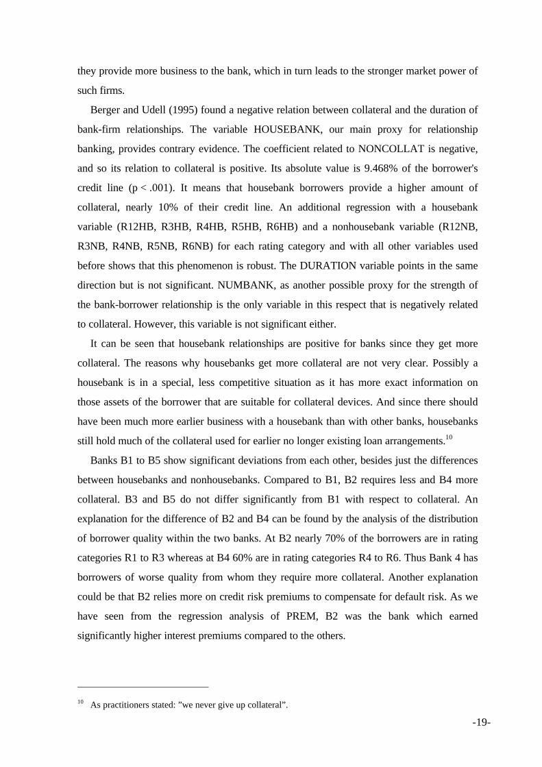
Berger and Udell (1995) found a negative relation between collateral and the duration of

bank-firm relationships. The variable HOUSEBANK, our main proxy for relationship

banking, provides contrary evidence. The coefficient related to NONCOLLAT is negative,

and so its relation to collateral is positive. Its absolute value is 9.468% of the borrower's

credit line (p < .001). It means that housebank borrowers provide a higher amount of

collateral, nearly 10% of their credit line. An additional regression with a housebank

variable (R12HB, R3HB, R4HB, R5HB, R6HB) and a nonhousebank variable (R12NB,

R3NB, R4NB, R5NB, R6NB) for each rating category and with all other variables used

before shows that this phenomenon is robust. The DURATION variable points in the same

direction but is not significant. NUMBANK, as another possible proxy for the strength of

the bank-borrower relationship is the only variable in this respect that is negatively related

to collateral. However, this variable is not significant either.

It can be seen that housebank relationships are positive for banks since they get more

collateral. The reasons why housebanks get more collateral are not very clear. Possibly a

housebank is in a special, less competitive situation as it has more exact information on

those assets of the borrower that are suitable for collateral devices. And since there should

have been much more earlier business with a housebank than with other banks, housebanks

still hold much of the collateral used for earlier no longer existing loan arrangements.10

Banks B1 to B5 show significant deviations from each other, besides just the differences

between housebanks and nonhousebanks. Compared to B1, B2 requires less and B4 more

collateral. B3 and B5 do not differ significantly from B1 with respect to collateral. An

explanation for the difference of B2 and B4 can be found by the analysis of the distribution

of borrower quality within the two banks. At B2 nearly 70% of the borrowers are in rating

categories R1 to R3 whereas at B4 60% are in rating categories R4 to R6. Thus Bank 4 has

borrowers of worse quality from whom they require more collateral. Another explanation

could be that B2 relies more on credit risk premiums to compensate for default risk. As we

have seen from the regression analysis of PREM, B2 was the bank which earned

significantly higher interest premiums compared to the others.

10 As practitioners stated: ”we never give up collateral”.

-20-

Other variables in this regression, such as the dummies for the certain years and the

variable on the day-to-day money rate, showed no significance. The adjusted R2 equals .204

which, though not as good as in the regression of premiums, but obviously significant

(F-value = 8.984 with a p-value below the .001 level). The other assumptions necessary to

allow appropriate OLS-estimations were again fulfilled.

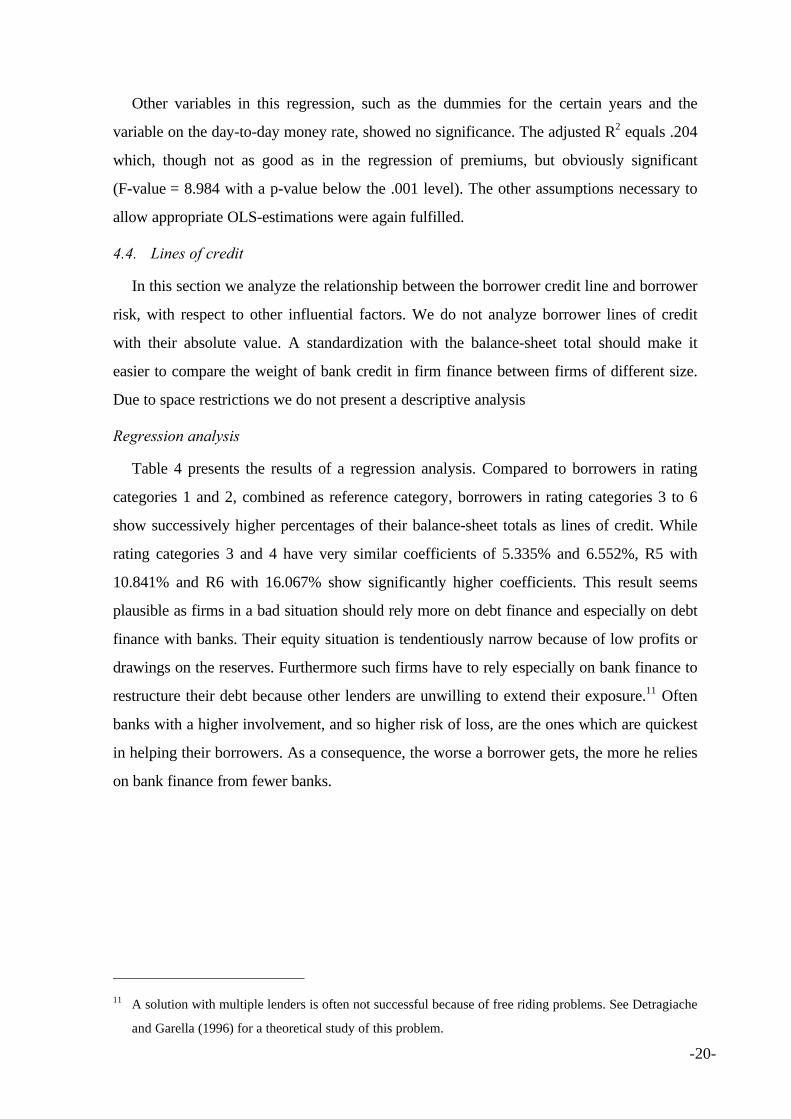
4.4. Lines of credit

In this section we analyze the relationship between the borrower credit line and borrower

risk, with respect to other influential factors. We do not analyze borrower lines of credit

with their absolute value. A standardization with the balance-sheet total should make it

easier to compare the weight of bank credit in firm finance between firms of different size.

Due to space restrictions we do not present a descriptive analysis

Regression analysis

Table 4 presents the results of a regression analysis. Compared to borrowers in rating

categories 1 and 2, combined as reference category, borrowers in rating categories 3 to 6

show successively higher percentages of their balance-sheet totals as lines of credit. While

rating categories 3 and 4 have very similar coefficients of 5.335% and 6.552%, R5 with

10.841% and R6 with 16.067% show significantly higher coefficients. This result seems

plausible as firms in a bad situation should rely more on debt finance and especially on debt

finance with banks. Their equity situation is tendentiously narrow because of low profits or

drawings on the reserves. Furthermore such firms have to rely especially on bank finance to

restructure their debt because other lenders are unwilling to extend their exposure.11 Often

banks with a higher involvement, and so higher risk of loss, are the ones which are quickest

in helping their borrowers. As a consequence, the worse a borrower gets, the more he relies

on bank finance from fewer banks.

11 A solution with multiple lenders is often not successful because of free riding problems. See Detragiache

and Garella (1996) for a theoretical study of this problem.

-21-

Table 4. Lines of credit as percentages of balance-sheet total


Intercept 20.335 .209


R3 5.335 .015

R4 6.552 .006

R5 10.841 .000

R6 16.067 .000

PREM .540 .565

NONCOLLAT -.025 .328

GUARANT -2.772 .184

DDRATE .313 .846


PARTNER 13.175 .000

PROP 14.471 .002


HOUSEBANK 12.206 .000

NUMBANK -.418 .020

DURATION -.079 .096


B2 1.727 .503

B3 -8.061 .003

B4 -3.939 .103

B5 -1.769 .514


Y3 -3.381 .393

Y4 -2.818 .677

Y5 -2.306 .775

Y6 -3.240 .741

BALANCE-SHEET TOTAL -2.872E-05 .000

Adjusted R2 = .259 (F = 10.894, p < .001)



A housebank should feel a special responsibility in such a situation. It has done a lot of

business with the borrower and intends to continue doing so in the future. The coefficient of

the HOUSEBANK variable supports this view. It indicates that a borrower with a

housebank relationship has a higher percentage of his balance-sheet total as credit line with

the housebank. An extended regression with a housebank variable and a nonhousebank

variable for each rating category shows that especially for borrowers in rating category 5

the housebank provides significantly more finance. The coefficient of R5HB has a value of

about 17% of the balance-sheet total which is a significant difference to nonhousebank-

-22-

borrowers of this category (p < .001). The coefficients of R3HB and R4HB are also

significant at this level but their values are only half of that of R5HB. For borrowers of

rating category 1 and 2 and for borrowers of rating category 6 there is no significant

difference between housebank-borrowers and nonhousebank-borrowers. In rating category

6 we find borrowers who move towards bankruptcy. In such a situation even the housebank

tries to cut lines and liquidate collateral. Thus no difference between housebank-borrowers

and nonhousebank-borrowers should be found. Contrarily, in rating category 5, the

housebank hopes to improve the situation with its help.

These results are consistent with the work of Hoshi, Kashyab and Scharfstein (1990, 1991).

They found that firms with close ties to a bank either in a keiretsu or in a relationship with a

main bank are less sensitive to liquidity in financing their investments, especially in times of

financial distress, because in contrast to capital markets banks are ready to provide more

debt.

There are also significant differences for borrowers with different legal forms.

Proprietorships and partnerships show a higher proportion of bank finance than

corporations. The coefficients of PROP and PARTNER have values of 14.471% (p = .002)

and 13.175% (p < .001).

Firm size is another factor which can explain differences in finance structure. In this

analysis the coefficient of the variable for the balance-sheet total of borrowers is significant

at better than the 1% level. Its value suggests that a borrower with a 200 million DM higher

balance-sheet total will have a credit line which is lower by 6% of its balance-sheet total.

Since the other variables in this analysis do not show significant values we do not discuss

them here.

The adjusted R2 of the regression model on lines of credit equals .259 which is a

significant value (F-value = 10.894, p-value below 001). The other assumptions necessary

to allow appropriate OLS-estimations were not violated.

5. Terms of lending and rating transition

In the previous Section we analyzed the relationship between terms of lending and

borrower risk. We found that the lower the borrower's quality, the higher the bank’s

premium. However, banks are ready to support the customers with whom they have a

housebank relationship when these customers have problems. What we are interested in

now is finding an answer to the question of how this behavior develops over time, especially

when borrower quality changes or, in formalized terms, when ratings migrate. We start by

-23-

describing rating transition. Then the variables used in the regression analysis will be

explained. The analysis is concentrated on the changes of interest rate premiums. Changes in

collateral and lines of credit do not show risk oriented behavior so the discussion of these

issues is rather narrow.

5.1. Rating transition

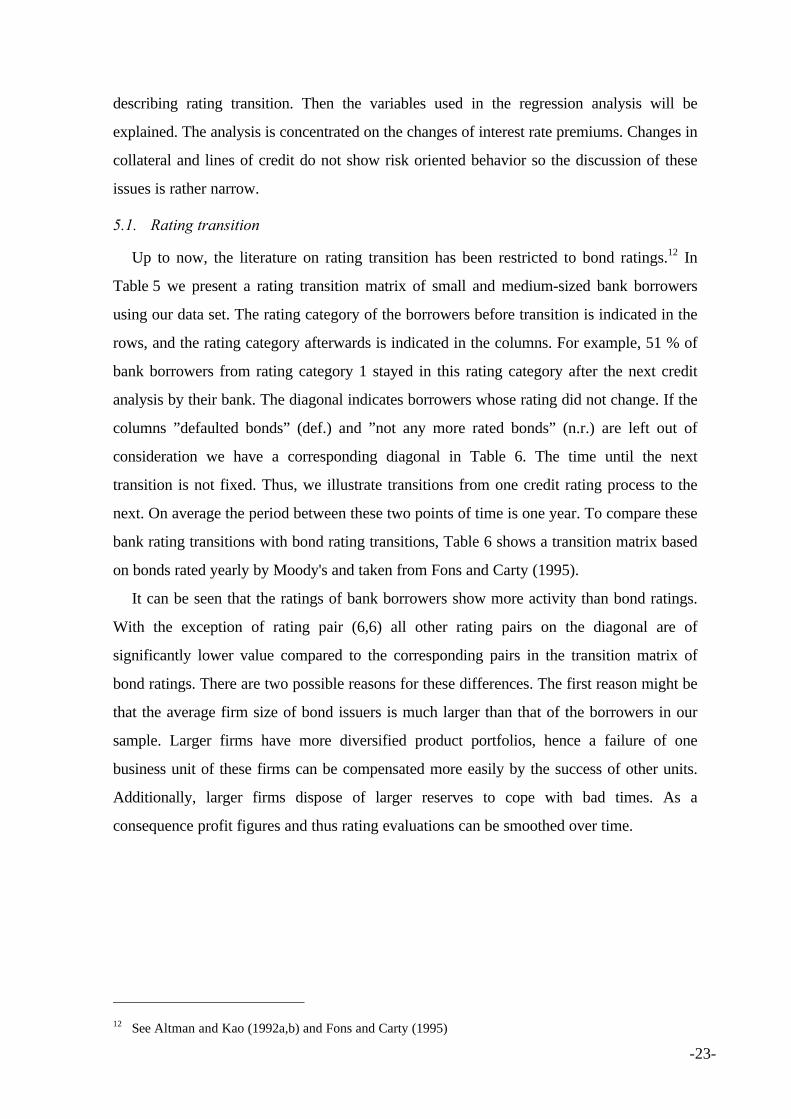
Up to now, the literature on rating transition has been restricted to bond ratings.12 In

Table 5 we present a rating transition matrix of small and medium-sized bank borrowers

using our data set. The rating category of the borrowers before transition is indicated in the

rows, and the rating category afterwards is indicated in the columns. For example, 51 % of

bank borrowers from rating category 1 stayed in this rating category after the next credit

analysis by their bank. The diagonal indicates borrowers whose rating did not change. If the

columns ”defaulted bonds” (def.) and ”not any more rated bonds” (n.r.) are left out of

consideration we have a corresponding diagonal in Table 6. The time until the next

transition is not fixed. Thus, we illustrate transitions from one credit rating process to the

next. On average the period between these two points of time is one year. To compare these

bank rating transitions with bond rating transitions, Table 6 shows a transition matrix based

on bonds rated yearly by Moody's and taken from Fons and Carty (1995).

It can be seen that the ratings of bank borrowers show more activity than bond ratings.

With the exception of rating pair (6,6) all other rating pairs on the diagonal are of

significantly lower value compared to the corresponding pairs in the transition matrix of

bond ratings. There are two possible reasons for these differences. The first reason might be

that the average firm size of bond issuers is much larger than that of the borrowers in our

sample. Larger firms have more diversified product portfolios, hence a failure of one

business unit of these firms can be compensated more easily by the success of other units.

Additionally, larger firms dispose of larger reserves to cope with bad times. As a

consequence profit figures and thus rating evaluations can be smoothed over time.

12 See Altman and Kao (1992a,b) and Fons and Carty (1995)

-24-

Table 5. Transition matrix of bank borrowers, 1992 to 1996, next credit analysis

from \ to 1 2 3 4 5 6 def. Observ.

1 51 40 9 0 0 0 0 100 % 35

2 8 62 19 8 2 1 0 100 % 103

3 0 8 69 17 6 0 0 100 % 226

4 1 1 10 64 21 3 0 100 % 222

5 0 1 2 19 66 12 0 100 % 137

6 0 0 0 2 16 70 12 100 % 58

Table 6. Transition matrix of bonds rated by Moody's, 1938-1993, one year (Fons and Carty 1995)

from \ to Aaa Aa A Baa Ba B Caa def. n.r.

Aaa 89.6 7.2 0.7 0.0 0.0 0.0 0.0 0.0 2.5 100 %

Aa 1.1 88.8 6.9 0.3 0.2 0.0 0.0 0.0 2.8 100 %

A 0.1 2.5 89.0 5.2 0.6 0.2 0.0 0.0 2.5 100 %

Baa 0.0 0.2 5.2 85.3 5.3 0.8 0.1 0.1 3.0 100 %

Ba 0.0 0.1 0.4 4.7 80.1 6.9 0.4 1.5 5.8 100 %

B 0.0 0.1 0.1 0.5 5.5 75.7 2.0 8.2 7.8 100 %

Caa 0.0 0.4 0.4 0.8 2.3 5.4 62.1 20.3 8.4 100 %

Secondly, because of long-term relationships banks have more inside information on

borrowers than any other outsider has. For this reason quality evaluations are more exact

and therefore ratings change more often. The underlying hypothesis is that analysts with less

exact information rely more on their previously assigned rating category by evaluating a

bond issuer. The percentage of defaulted bank borrowers, which is lower than that of

defaulted bonds, suggests that banks are more ready to support their customers in times of

distress. Thus the higher percentage of borrowers who stay in rating category 6 is

explainable.

5.2. Variables

The variables used are illustrated in Table 7. Also included are bank dummies B1 to B5,

which were described in Section 4.

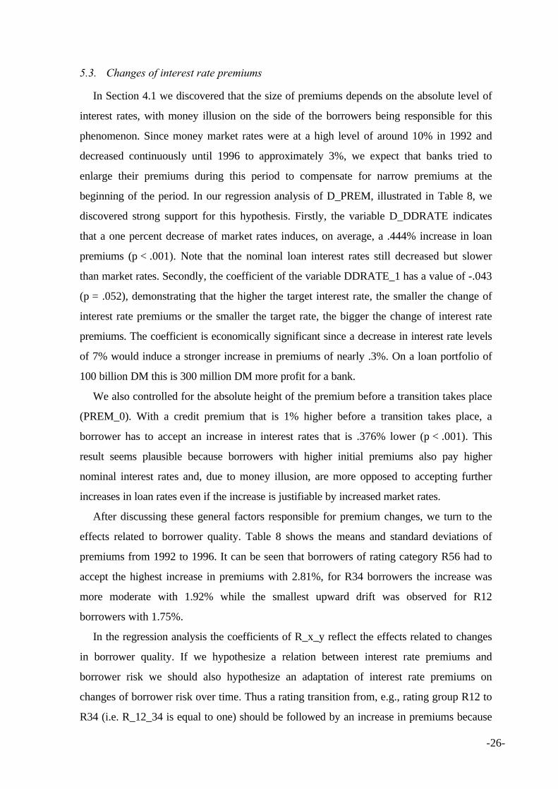
The variable D_PREM is defined as the change of the loan interest rate premium during

a transition, i.e. the time between two consecutive credit analyses by the bank. Its value

represents a change in absolute percentages. The previous premium is denoted by PREM_0.

A "0" as suffix indicates that a value belongs to the time before a transition takes place, and

a "1" indicates that a value belongs to the time afterwards.

-25-

We suppose that changes in collateral can also affect premium adaptation. Hence

D_NONCOLLAT, i.e. the change in the unsecured percentage of the borrower's credit line,

is included in the analysis. Again, its value represents a change in absolute percentages.

The variable L/C_1 denotes in thousands of deutschmarks (TDM) the line of credit of a

borrower after a transition. This variable should account for differences effected by the size

of business.

Table 7. Variable description

Variable Description

Contract

D_PREM Change in loan interest rate premium (percentage points)

PREM_0 Premium before transition (%)

D_NONCOLLAT Change in unsecured percentage of credit line (percentage points)

L/C_1 Line of credit after transition (TDM)

Market

D_DDRATE Change in Day-to-day interbank money rate (percentage points)

DDRATE_1 Day-to-day interbank money rate after transition (%)

Risk

Rx = 1 if borrower was in rating category group x before transition

Ry = 1 if borrower was in rating category group y after transition

R_x_y = 1 if borrower was in rating category group x before transitionand is in rating category group y afterwards

The change in the day-to-day money rate (D_DDRATE) is an exogenous variable in the

regression because it should be expected that changes in market rates and thus in

refinancing costs for the bank affect its interest rate offers for loans. To control for the

absolute level of interest rates DDRATE_1, the market rate after a transition, is also taken

into consideration. As mentioned above, we think that money illusion is an important factor

for loan pricing. Thus high nominal interest rate levels will restrict banks from enlarging

their premiums whereas low rates will encourage them to require higher premiums.

The most important variables are the dummies on rating transitions. In order not to

overload our regression analysis we pooled our rating categories into three groups of rating

pairs, (1,2), (3,4) and (5,6), qualitatively expressed as good, normal and bad borrowers. As

a consequence we only have 9 variables which represent rating transition. In general terms,

R_x_y is a rating dummy which has a value of one if the borrower was of rating group Rx

before and of rating group Ry after the transition, with Rx and Ry of the set of rating

category groups {(1,2), (3,4), (5,6)} respectively. R_x_y is zero otherwise. In the following

we also denote the dummy variables on rating category groups with R12, R34 and R56.

-26-

5.3. Changes of interest rate premiums

In Section 4.1 we discovered that the size of premiums depends on the absolute level of

interest rates, with money illusion on the side of the borrowers being responsible for this

phenomenon. Since money market rates were at a high level of around 10% in 1992 and

decreased continuously until 1996 to approximately 3%, we expect that banks tried to

enlarge their premiums during this period to compensate for narrow premiums at the

beginning of the period. In our regression analysis of D_PREM, illustrated in Table 8, we

discovered strong support for this hypothesis. Firstly, the variable D_DDRATE indicates

that a one percent decrease of market rates induces, on average, a .444% increase in loan

premiums (p < .001). Note that the nominal loan interest rates still decreased but slower

than market rates. Secondly, the coefficient of the variable DDRATE_1 has a value of -.043

(p = .052), demonstrating that the higher the target interest rate, the smaller the change of

interest rate premiums or the smaller the target rate, the bigger the change of interest rate

premiums. The coefficient is economically significant since a decrease in interest rate levels

of 7% would induce a stronger increase in premiums of nearly .3%. On a loan portfolio of

100 billion DM this is 300 million DM more profit for a bank.

We also controlled for the absolute height of the premium before a transition takes place

(PREM_0). With a credit premium that is 1% higher before a transition takes place, a

borrower has to accept an increase in interest rates that is .376% lower (p < .001). This

result seems plausible because borrowers with higher initial premiums also pay higher

nominal interest rates and, due to money illusion, are more opposed to accepting further

increases in loan rates even if the increase is justifiable by increased market rates.

After discussing these general factors responsible for premium changes, we turn to the

effects related to borrower quality. Table 8 shows the means and standard deviations of

premiums from 1992 to 1996. It can be seen that borrowers of rating category R56 had to

accept the highest increase in premiums with 2.81%, for R34 borrowers the increase was

more moderate with 1.92% while the smallest upward drift was observed for R12

borrowers with 1.75%.

In the regression analysis the coefficients of R_x_y reflect the effects related to changes

in borrower quality. If we hypothesize a relation between interest rate premiums and

borrower risk we should also hypothesize an adaptation of interest rate premiums on

changes of borrower risk over time. Thus a rating transition from, e.g., rating group R12 to

R34 (i.e. R_12_34 is equal to one) should be followed by an increase in premiums because

-27-

the default is more probable in R34 compared to R12. On the other hand, a rating transition

from R56 to R34 (i.e. R_56_34 is equal to one) should induce a decline in premiums, and

an affirmation of a rating category should be accompanied by stability of premiums. The

regression analysis (see Table 8) does not support the hypothesis of a relation between

changes of loan premiums and credit ratings. With R_12_12 as reference, the coefficientss

of R_12_34 and R_12_56 do not differ significantly from zero while the coefficients

R_34_y and R_56_y, y of {(1,2),(3,4),(5,6)}, do differ significantly. Additional tests on the

differences of the dummy coefficients show that there is no significant difference between

the variables within the group of R_56_y. Within the group R_34_y the coefficient of

R_34_56 indicates a significantly higher premium change (p = .069) compared to R_34_34,

while there is no significant deviation of R_34_56 from R_56_34. Thus it seems that

borrowers of the R34_56 group are rather treated as borrowers of the R_56_y group. In

general these results show that in the observed period of 1992 to 1996 there was no

accurate adjustment of premiums to borrower risk changes.

According to the above evidence we conclude that in the observed period banks

primarily intended to enlarge their premiums based on their negotiation power. This

negotiation power was high if the borrower was of bad quality and low if the borrower was

of good quality.

Table 8. Loan premiums within rating categories R12, R34 and R56 from 1992 to 1996

R12 R34 R56

Year Mean Std. dev. Mean Std. dev Mean Std. dev.

1992 2.14 .59 2.33 .75 2.48 1.18

1993 3.08 .57 3.42 .90 3.71 1.31

1994 3.72 .76 3.93 .90 4.56 .97

1995 3.59 .78 4.06 .95 4.79 1.10

1996 3.89 .92 4.25 1.08 5.29 1.11

Increase 1.75 1.92 2.81

To support the above conclusion, we ran another two regressions of changes in interest

rate premiums. In these regressions the dummies R_x_y were omitted. In the first regression

we introduced the dummies R_x_0 instead to test for possible relations of premium changes

solely on the adherence to a certain rating group, i.e. R12, R34 or R56, before a transition

takes place. In the second regression we introduced R_y_1 to test for the same relation but

after a transition has taken place. The results were significant (p < .01) suggesting that

banks define their negotiation power by the status of the borrower belonging to a certain

-28-

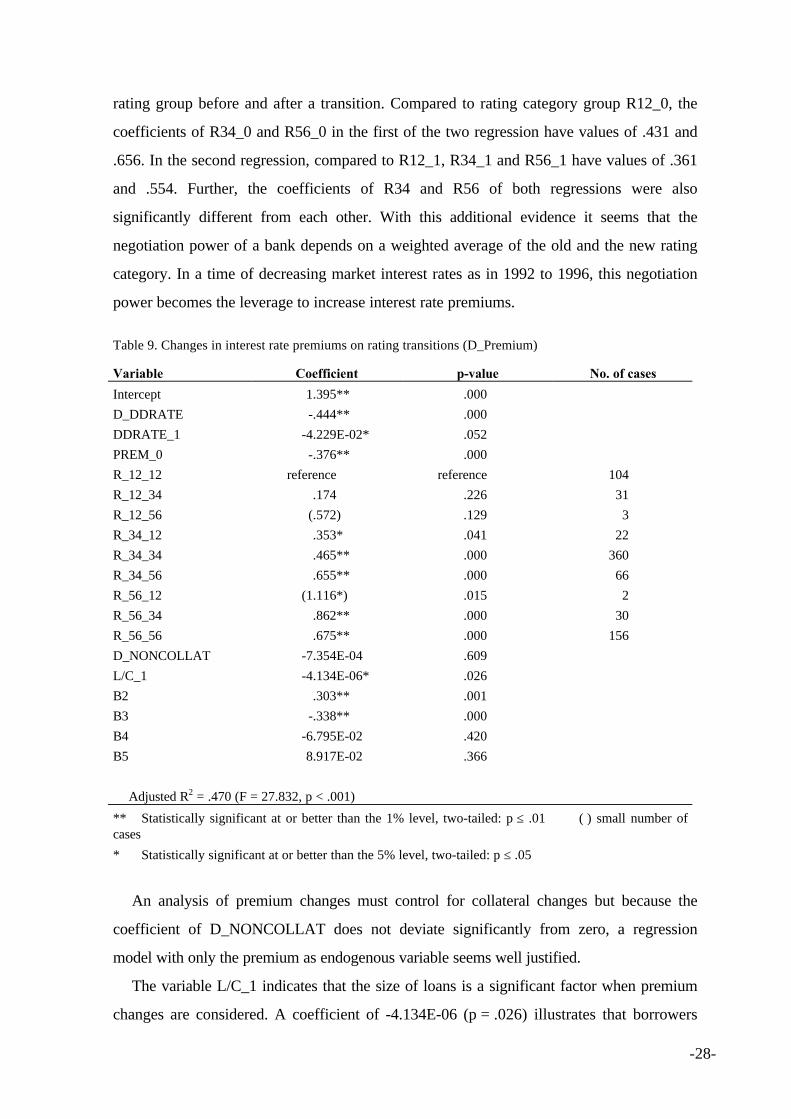
rating group before and after a transition. Compared to rating category group R12_0, the

coefficients of R34_0 and R56_0 in the first of the two regression have values of .431 and

.656. In the second regression, compared to R12_1, R34_1 and R56_1 have values of .361

and .554. Further, the coefficients of R34 and R56 of both regressions were also

significantly different from each other. With this additional evidence it seems that the

negotiation power of a bank depends on a weighted average of the old and the new rating

category. In a time of decreasing market interest rates as in 1992 to 1996, this negotiation

power becomes the leverage to increase interest rate premiums.

Table 9. Changes in interest rate premiums on rating transitions (D_Premium)

Variable Coefficient p-value No. of cases

Intercept 1.395** .000

D_DDRATE -.444** .000

DDRATE_1 -4.229E-02* .052

PREM_0 -.376** .000

R_12_12 reference reference 104

R_12_34 .174 .226 31

R_12_56 (.572) .129 3

R_34_12 .353* .041 22

R_34_34 .465** .000 360

R_34_56 .655** .000 66

R_56_12 (1.116*) .015 2

R_56_34 .862** .000 30

R_56_56 .675** .000 156

D_NONCOLLAT -7.354E-04 .609

L/C_1 -4.134E-06* .026

B2 .303** .001

B3 -.338** .000

B4 -6.795E-02 .420

B5 8.917E-02 .366

Adjusted R2 = .470 (F = 27.832, p < .001)

** Statistically significant at or better than the 1% level, two-tailed: p ≤ .01 ( ) small number ofcases


An analysis of premium changes must control for collateral changes but because the

coefficient of D_NONCOLLAT does not deviate significantly from zero, a regression

model with only the premium as endogenous variable seems well justified.

The variable L/C_1 indicates that the size of loans is a significant factor when premium

changes are considered. A coefficient of -4.134E-06 (p = .026) illustrates that borrowers

-29-

whose credit line is 50 million DM higher at the time after a transition have to accept an

increase in premiums that is 20 basis points weaker on average.

The analysis of the individual banks shows that, compared to B1, B2 was more able to

increase loan premiums, with a coefficient of the related dummy variable of .303 (p = .001).

Contrarily, B3 had to accept weaker increases, compared to B1, with a coefficient of -.338

(p < .001).

Extensions of the above regression model with other variables used in Section 4 showed

no significant results. In order not to overload the estimation procedure we left them out.

The regression model used here to explain premium changes seems well determined as the

multiple coefficient of determination R2 has a value of .470 (F-value = F = 27.832, p-value

below .001). The usual assumptions allowing for an OLS-estimation were fulfilled.

5.4. Changes of collateral and lines of credit

Two regressions, one with the change of the unsecured percentage of the borrower's

credit line (D_NONCOLLAT) and one with the change in the lines of credit (D_L/C) as

endogenous variable, show no link to levels or changes of borrower risk. The fact that there

is a negative relation of both kinds of changes to their basis value, i.e. the value before a

transition takes place, attributes a certain plausibility to the analysis.

Furthermore the coefficient of D_LC in the regression of D_NONCOLLAT is positive at

the better than 1% level, indicating that D_NONCOLLAT is significantly determined by

D_LC. Obviously, changes in the lines of credit change the unsecured percentage of credit

lines. This is plausible because collateral is the debt parameter which should be most

stagnant.

6. Conclusion

This paper provides evidence for the relation of loan terms to borrower risk. We found

that loan interest rate premiums and lines of credit are related to borrower credit ratings

while collateral showed no clear relation. An analysis of changes in loan interest rate

premiums, collateral and lines of credit gave no hint to an adjustment of loan terms on

rating transitions, suggesting that, in the period under study, there should be a deterioration

of the relation of loan terms to borrower ratings over time.

Money illusion was found as another important factor explaining levels and changes of

loan interest rate premiums. No evidence for the influence of relationship banking was

found. Yet, for collateral and lines of credit the HOUSEBANK variable as proxy of the

-30-

bank-borrower relationship was significant. Relative to granted lines of credit, housebanks

get a higher percentage of collateral and, in relation to their customers’ balance-sheet totals,

such banks provide higher credit lines. Compared to earlier results, the findings on lines of

credit are consistent with the existing literature. The findings on collateral are not.

Theoretical work such as that of Boot and Thakor (1994) and empirical work such as that

of Berger and Udell (1995) make opposing statements when collateral is considered. We

can explain this phenomenon only by the fact that a housebank, better than others, uses its

information advantage to more easily discover assets which may be used as collateral or that

it still has collateral in its portfolio which were used for earlier loan arrangements that are

not existent any more. Statements of different banks support the latter point.

Besides relationship banking the legal form of borrowers is another factor for the level of

collateral related to lines of credit and lines of credit related to borrowers' total assets.

Noncorporations have to provide more collateral but therefore lines of credit are a more

important source of finance for them.

An appropriate adjustment of loan terms on rating transitions could not be discovered.

While the analysis of changes in collateral and lines of credit do not indicate any link to

rating transitions, the analysis of changes in loan premiums suggests that banks define their

market power on a weighted average of the rating category just before and after a rating

transition. Based on that market power, they raised their premiums in a period from 1992 to

1996 when market interest rates fell from nearly 10% to 3%. Thus money illusion on the

side of the borrowers plays a key role. For a more detailed statement our data basis would

have to be broader. While there are many cases with stable ratings there are few with rating

changes. Additionally, our design only considers changes after one transition and therefore

could be too myopic. Again, to widen the horizon of the analysis more data would be

necessary. In particular, the period under study and jointly the number of transitions must be

increased. Furthermore, it should not be forgotten that within the period from 1992 to 1996

market interest rates fell continuously. A next study on premium changes should include

data of a period with increasing market rates.

-31-

Acknowledgements

This research is part of the project "Credit Management in Germany" at the Center for

Financial Studies in Frankfurt. We thank all the participating banks and research groups for

their support in gathering the data and for the intensive discussion on that project. In

particular we thank Herbert Hampl, Martin Hellendahl, Reinhard Kutscher, Hans-Jürgen

Oswald, Otto Steinmetz and Bernd Zugenbühler on the banks’ side. On the side of the

research groups we thank Peter Burghof, Ralf Elsas, Ralf Ewert, Sabine Henke, Jan Pieter

Krahnen, Bernd Rudolph and Gerald Schenk. We also appreciate helpful suggestions from

Thomas Langer, Gunter Löffler, Susanne Prantl and Frank Vossmann.

-32-

References

Altman, E.I., Kao, D.L., 1992a. Rating drift in high-yield bonds. The Journal of Fixed

Income, March issue, 15-20.

Altman, E.I., Kao, D.L.,1992b. The implications of corporate bond ratings drift. Financial

Analysts Journal, May-June issue, 64-75.

Berger, A.N., Udell, G.F., 1990. Collateral, Loan Quality, and Bank Risk. Journal of

Monetary Economics 25, 21-42.

Berger, A.N., Udell, G.F.,1992. Some evidence on the empirical significance of credit

rationing. Journal of Political Economy 100, 1047-1077.

Berger, A.N., Udell, G.F., 1995. Relationship lending and lines of credit in small firm

finance. Journal of Business 68, 351-381.

Berlin, M., Mester, L.J., 1997. On the profitability and cost of relationship lending,

Working Paper no. 97-3/R, Federal Reserve Bank of Philadelphia.

Besanko, D., Thakor, A.V., 1987. Collateral and Rationing: Sorting Equilibria in

Monopolistic and Competitve Credit Markets. International Economic Review 75, 850-

855.

Bester, H., 1985. Screening vs. rationing in credit markets with imperfect information.

American Economic Review 75, 850-855.

Blackwell, D.W., Winters, D.B., 1997. Banking relationships and the effect of monitoring in

loan pricing. The Journal of Financial Research 20, 275-289.

Boot, A.W.A., Thakor, A.V., 1994. Moral hazard and secured lending in an infinitely

repeated credit market game. International Economic Review 35, 899-920.

Detragiache, E., Garella, P.G., 1996. Debt restructuring with multiple creditors and the role

of exchange offers. Journal of Financial Intermediation 5, 305-336

Edwards, J.S.S., Fischer, K., 1994. Banks, finance and investment in Germany, University

Press, Camebridge.

Elsas, R., Henke, S., Machauer, A., Rott, R., Schenk, G., 1997. Empirische Untersuchung

von Kreditengagements mittelständischer Unternehmen - Samplingkonzeption und

deskriptive Statistik, Working Paper, Center for Financial Studies, Frankfurt.

Elsas, R., Krahnen, J.P., 1998. Is relationship lending special ? Evidence from credit-file

data in Germany, Working Paper no. 98/01, Center for Financial Studies, Frankfurt a.M.,

Germany.

-33-

Fischer, K., 1990. Hausbankbeziehungen als Instrument der Bindung zwischen Banken und

Unternehmen - Eine theoretische und empirische Analyse, Ph.D. thesis, Bonn, Germany.

Fisher, I., 1928. The Money Illusion, Adelphi, New York.

Fons, J.S., Carty, L.V., 1995. Probability of default: a derivatives perspective, in: Risk

Publications: Derivative credit risk - advances in measurement and management,

London, 35-47.

Fried, J., Howitt, P. 1980. Credit rationing and implicit contract theory. Journal of Money,

Credit, and Banking 12, 471-487.

Gorton, G., Kahn, J., 1996. The design of bank loan contracts, collateral, and renegotiation,

Working Paper no. 4273, National Bureau of Economic Research.

Greenbaum, S.I., Kanatas, G., Venezia, I., 1989. Equilibrium loan pricing under the bank-

client relationship. Journal of Banking and Finance 13, 221-235.

Hoshi,T., Kashyab, A., Scharfstein, D., 1990. The role of banks in reducing the costs of

financial distress in Japan. Journal of Financial Economics 27, 67-88.

Hoshi, T., Kashyab, A., Scharfstein, D., 1991. Corporate structure, liquidity, and

investment: evidence from japanese industrial groups. Quarterly Journal of Economics

106, 33-60.

Mayer, C., 1988. New issues in corporate finance. European Economic Review 32, 1167-

1189.

Petersen, M.A., Rajan, R.G., 1994. The benefits of lending relationships: evidence from

small business data. Journal of Finance 49, 3-37.

Petersen, M.A., Rajan, R.G., 1995. The effect of credit market competition on lending

relationships. Quarterly Journal of Economics 110, 407-443.

Saunders, A., 1997. Financial institutions management: a modern perspective, 2nd ed., Irwin,

Chicago.

Shafir, E., Diamond, P., Tversky, A., 1997. Money Illusion. Quarterly Journal of

Economics 112, 341-374.

Sharpe, S. A., 1990. Asymmetric Information, Bank Lending, and Implicit Contracts: A Stylized

Model of Customer Relationships. The Journal of Finance 45, 1069-1087.

Stiglitz, J.E., Weiss, A., 1981. Credit Rationing in markets with imperfect information.

American Economic Review 71, 393-410.

Thaler, R., 1992. The Winner’s Curse, The Free Press, New York.

Bank behavior based on internal credit ratings of … behavior based on internal credit ratings of...

Documents

Transcript of Bank behavior based on internal credit ratings of … behavior based on internal credit ratings of...