Bang-bang Control Design by Combing Pseudospectral

Method with a novel Homotopy Algorithm

Xiaoli Bai∗, James D. Turner†, John L. Junkins‡

Texas A&M University, College Station, Texas 77843

Abstract

The bang-bang type of control problem for spacecraft trajectory optimization is solved by

using a hybrid approach. First, a pseudospectral method is utilized to generate approximate

switching times, control structures, and initial co-states. Second, a homotopy method is used

to solve the two-point boundary value problems derived from the Euler-Lagrangian equations.

The unknown variables in the homotopy method include both switching times and the unknown

initial states and co-states. The homotopy algorithm is made robust to the nonlinearity of the

problems by enforcing the constraint satisfaction along the homotopy path. The optimization

variables are treated as continuous variables and the final solutions have the same accuracy as

the ordinary differential equation solvers. An orbit transfer problem is presented to show the

advantages of this hybrid methodology.

∗Current Affiliation:Graduate Research Assistant, Department of Aerospace Engineering, TAMU-3141; xi-aolibai@tamu.edu; phone: 979-862-3394; fax: 979-845-6051. Student Member AIAA.

†Research Professor, Department of Aerospace Engineering, TAMU-3141; Associate Fellow AIAA‡Regents Professor, Distinguished Professor of Aerospace Engineering, Holder of the Royce E. Wisenbaker ’39

Chair in Engineering, Department of Aerospace Engineering, TAMU-3141. Fellow AIAA.

1

1 Introduction

A classical subject in optimal control fields is the bang-bang type of control problems.1 These

problems often arise when the constrained control appears linearly in both the state differential

equations and the performance function while the final time can be either free or fixed. For ex-

ample, the solution of time optimal three-axis reorientation of a rigid body is usually a bang-bang

controller2,.3 The low thrust spacecraft trajectory design with the aim to minimize the fuel con-

sumption, which is equivalent to maximizing the final mass, also frequently leads to bang-bang

controls, or thrusting and coasting type of controls4,.5 The bang-bang control for low thrust trajec-

tory optimization is of particular interest in this paper.

The computational techniques to solve optimal control problems are either indirect shooting

or direct shooting.6 The direct methods introduce a parametric representation of the control vari-

ables (and frequently the state variables as well), and then resort to optimizers such as ‘fmincon’

in MATLAB, SNOPT,7 or SOCS8 to solve the resulting nonlinear programming problems.9 With

the increasing power of these optimizers, it is possible to discretize the continuous system by using

very small step. For example, Betts and Erb9 used a collocation or direct transcription method

to design an optimal low thrust trajectory to the moon through SOCS software.8 Their final non-

linear programs include 211031 variables and 146285 constraints. Usually the direct approach is

robust to the initial guess for the problem. Since there is no need to derive for the Euler-Lagrange

equations,1 it is easy to automate the direct transcription process so this direct method has special

interest in industry, leading to some example software such as POST and GTS.6 Although the di-

rect approaches have been very attractive to solve orbit transfer problems with impulses burns,10

for low thrust propulsion where the thrust level is low relative to the spacecraft mass, the inte-

2

grated trajectory using the interpolated control from the direct approach can drift from the optimal

trajectory and the optimality is difficult to guarantee.

Indirect approaches are based on the calculus of variations. Necessary conditions are derived

from Pontryagin’s principles.1 A simple shooting or multiple shooting method is usually used

to solve the resulting two-point value problems, with the goal to find the unknown initial states

and co-states. This method is not popular in industry because of the difficulty encountered in

automating the process to translate the original problem to a two-point boundary value problem.

However, mathematical programming languages such as AMPL and the automatic differentiation

techniques have made automation of this process possible11,12,.13 The solutions obtained from the

indirect approach assure the optimality and accuracy, which is the main reason why this method

has been very popular for low thrust trajectory design4,14,15,.16 The greatest difficulty encountered

with this approach is that it is very sensitive to the initial guess; this problem is because that for the

state equation and co-state equations resulting from the Euler-Lagrange equations, one of them is

stable to integrate forward while the other one is stable only if it is integrated backward from the

final time.17

The small convergence domain issue becomes even more difficult for solving bang-bang type of

control problems using the indirect approach for two reasons. First, the control is non-differentiable,

creating the possibility that the Jacobian matrix, which is required to compute when gradient or

Newton’s based methods18 are used to solve the two-point boundary values problems, may become

singular on a large domain. Second, discontinuous control makes it difficult for most available or-

dinary differential equation solvers to generate high accuracy solutions if the switching times are

not known at prior. Additionally, as mentioned Bai and Junkins3 and Bskens,19 the current knowl-

edge about the second order sufficient conditions for these bang-bang control problems is still

3

limited. Maurer and Osmolovskii20 provided a systematic numerical method to verify the second

order conditions. In the case of one or two switches, the tests are very easy to implement. The

authors precluded simultaneous switching bang-bang control structures when they derived the sec-

ond order conditions. However, simultaneous switching cases are found quite often for the three

axis rigid body maneuver.3 Bertrand and Epenoy5 used new smoothing techniques to solve bang-

bang optimal control problems. The authors studied different type of perturbation terms that can

be added to the objective function to improve the convergence domain of the Newton’s method to

solve such problems. For an Earth to Venus problem, where the possible global optimal trajectory

includes six switches, the authors showed that the convergence rate is less than 10% when using a

hundred different starting points.

Because of the pros and cons of both direct and indirect approaches, combing them to solve

complicated problems has been very successful3,21,.22 Usually, the co-states and control structure

information is first extracted from a nonlinear programming approach. The solutions are refined

by using an indirect shooting method. Although hybrid approaches are usually very effective

to expand the convergence domain for the indirect methods and increase the accuracy for the

direct methods, both efficient direct algorithm and quality indirect method are required to solve

complicated problems.

A Legendre pseudospectral method is chosen as the direct shooting algorithm in this paper.

Pseudospectral methods were initially used widely in fluid dynamics,23 and has become a very

active research field in recent years24,25,26,.27 Ross et al.26 claimed that the pseudospectral method

is able to solve low thrust trajectory optimization problems with high accuracy. However, we

believe there is no guarantee that the integrated trajectory using the control obtained from the

pseudospectral methods through interpolation is the real optimal solution. This issue is addressed

4

in the next section and further demonstrated in the application section.

The accuracy of the direct solutions is improved through an indirect approach, by introduc-

ing a novel homotopy method in the paper. To solve optimization problems when using homotopy

method , researchers either construct a continuation algorithm or use the probability-one homotopy

algorithm. 28,29,30 The probability-one homotopy algorithm parameterizes both the state variables

and the homotopy variable as functions of arc length such that the homotopy variable can both

increase and decrease. Previous published homotopy strategy translates the problem into a one-

parameter chain of problems. The starting reference problem is easy to solve, and its solution

serves as the initial guess for the next problem. By changing the marching parameter variable(the

homotopy variable), this process is continued until the objective problem is reached and solved.

This strategy is discussed in detail when Bulirsch, Montrone and Pesch used it to solve a compli-

cated control problem of abort landing of a passenger aircraft in the presence of windshear .31,32

The homotopy algorithm utilized in this paper was developed by Bai, Junkins, and Turner33,34

and is different from the traditional approaches. Instead of solving a chain of problems, the pro-

posed homotopy method solves just one problem. The algorithm starts from some initial guess

to the problem and ends at the final accurate local optimal solutions. The homotopy method was

demonstrated to solved several algebraic optimization problems which are beyond the capabilities

of ‘fmincon’33 first. They further designed unconstrained optimal thrust direction for an Earth to

Apophis rendezvous problem.34 For the cases that can not be solved using SNOPT, their homo-

topy algorithm encounters no problems. This current paper extends the pervious two papers to

solve bang-bang control problems using the homotopy methodology.

The organization of this paper is as follows. Section 2 briefly describes the pseudospectral

method and discusses the problems that may be encountered if the user only depends on pseu-

5

dospectral method to generate high accurate solutions, especially for low thrust problems. Sec-

tion 3 first presents the mathematical equations of the optimal control problems, which are formu-

lated for solutions by the homotopy method. The homotopy algorithm is presented for rigorously

tracking equality constraints. An orbit rendezvous problem is presented in Section 4. The pro-

cedures to solve the problem and simulation results are discussed. Conclusion remarks follow in

Section 5.

2 Approximate Solution by Using a Psedospectral Method

Psedospectral methods use Lagrange form of the interpolation polynomials to describe states.

For a given set of N +1 data points t0, t1, t2, · · · , tN , the Lagrangian basis polynomials are defined

as

φi(t) =k=N∏

k=0,k 6=i

t− tkti − tk

, i = 0, 1, · · · , N (1)

To overcome the Runge’s phenomenon and utilize the quadrature rules for integration, the roots

of orthogonal polynomials are usually chosen as the psedospectral nodes, leading to the methods

such as Chebyshev pseudospectral methods and Legendre pseudospectral methods. Comparing

with Chebyshev polynomial methods,24 Legendre pseudospectral method with Legendre-Gauss-

Lobatto (LGL) nodes27 are chosen in the paper since the well established co-vector mapping theo-

rem provides the proper connection to commute dualization with discretization.27 For LGL nodes,

ti, 1 ≤ i ≤ N are chosen as the zeros of the derivative of the Legendre polynomials of order N

with t0 = −1 and tN = 1. The state variables are approximated by using N th order interpolation

6

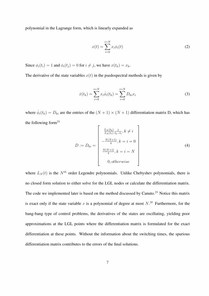
polynomial in the Lagrange form, which is linearly expanded as

x(t) =i=N∑i=0

xiφi(t) (2)

Since φi(ti) = 1 and φi(tj) = 0 for i 6= j, we have x(tk) = xk.

The derivative of the state variables x(t) in the psedospectral methods is given by

x(tk) =i=N∑i=0

xiφi(tk) =i=N∑i=0

Dkixi (3)

where φi(tk) = Dki are the entries of the (N + 1) × (N + 1) differentiation matrix D, which has

the following form23

D := Dki =

LN (tk)LN (ti)

1tk−ti

, k 6= i

−N(N+1)4

, k = i = 0

N(N+1)4

, k = i = N

0, otherwise

(4)

where LN(t) is the N th order Legendre polynomials. Unlike Chebyshev polynomials, there is

no closed form solution to either solve for the LGL nodes or calculate the differentiation matrix.

The code we implemented later is based on the method discussed by Canuto.23 Notice this matrix

is exact only if the state variable x is a polynomial of degree at most N .35 Furthermore, for the

bang-bang type of control problems, the derivatives of the states are oscillating, yielding poor

approximations at the LGL points where the differentiation matrix is formulated for the exact

differentiation at these points. Without the information about the switching times, the spurious

differentiation matrix contributes to the errors of the final solutions.

7

Although the mesh refinement techniques27 or removing the Gibbs phenomenon by some fil-

tering procedures23 can relieve these problems to some extend, to guarantee the accuracy and opti-

mality of the solutions, we utilize a robust homotopy method to find the optimal solution through

an indirect approach.

3 Indirect Solution by Using a Novel Homotopy Method

3.1 Problem Formulation

The mathematical equations of the optimal control problems are formulated for solutions by the

homotopy method. The equations of motion for a general dynamic system with control appearing

linearly can be written as

x = f(t) = A(x, t)x + B(x, t)u + C(f ∈ Rn,u ∈ Rm) (5)

where A and B can be both time-varying and dependent on x(t); C is a constant force vector.

Using perturbation methods,36 the solution of Eq. 5 is given by

x(t) = φ(t, 0)x(0) + φ(t, 0)

∫ t

0

φ−1(τ, 0)(AQ + Bu)dτ + Q (6)

with

Q = C (7)

8

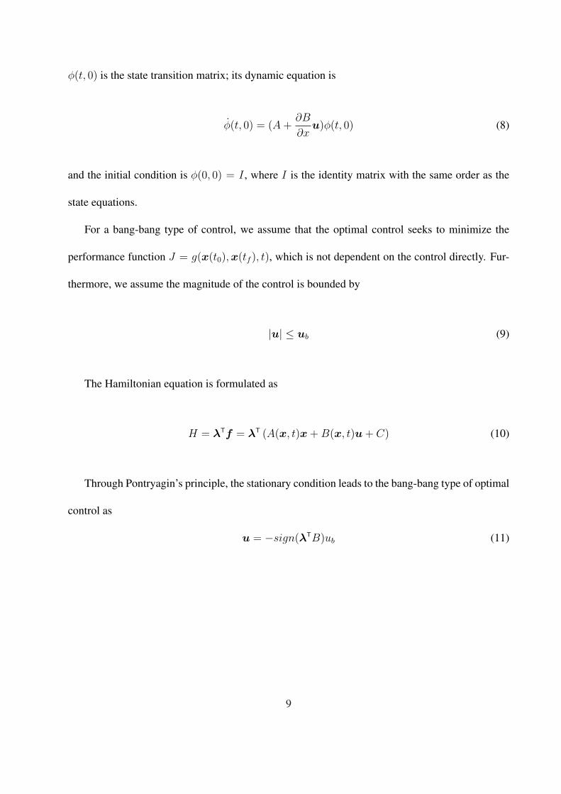
φ(t, 0) is the state transition matrix; its dynamic equation is

φ(t, 0) = (A +∂B

∂xu)φ(t, 0) (8)

and the initial condition is φ(0, 0) = I , where I is the identity matrix with the same order as the

state equations.

For a bang-bang type of control, we assume that the optimal control seeks to minimize the

performance function J = g(x(t0), x(tf ), t), which is not dependent on the control directly. Fur-

thermore, we assume the magnitude of the control is bounded by

|u| ≤ ub (9)

The Hamiltonian equation is formulated as

H = λTf = λT (A(x, t)x + B(x, t)u + C) (10)

Through Pontryagin’s principle, the stationary condition leads to the bang-bang type of optimal

control as

u = −sign(λTB)ub (11)

9

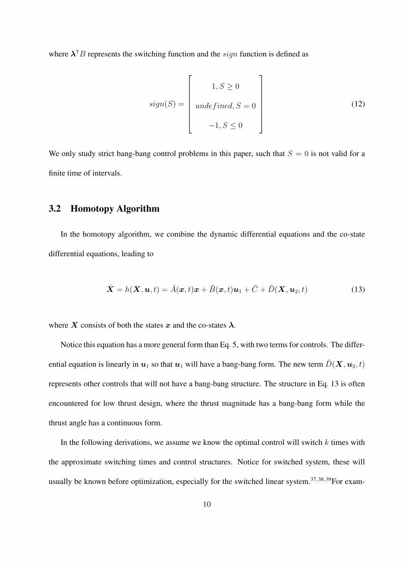
where λTB represents the switching function and the sign function is defined as

sign(S) =

1, S ≥ 0

undefined, S = 0

−1, S ≤ 0

(12)

We only study strict bang-bang control problems in this paper, such that S = 0 is not valid for a

finite time of intervals.

3.2 Homotopy Algorithm

In the homotopy algorithm, we combine the dynamic differential equations and the co-state

differential equations, leading to

X = h(X,u, t) = A(x, t)x + B(x, t)u1 + C + D(X,u2, t) (13)

where X consists of both the states x and the co-states λ.

Notice this equation has a more general form than Eq. 5, with two terms for controls. The differ-

ential equation is linearly in u1 so that u1 will have a bang-bang form. The new term D(X,u2, t)

represents other controls that will not have a bang-bang structure. The structure in Eq. 13 is often

encountered for low thrust design, where the thrust magnitude has a bang-bang form while the

thrust angle has a continuous form.

In the following derivations, we assume we know the optimal control will switch k times with

the approximate switching times and control structures. Notice for switched system, these will

usually be known before optimization, especially for the switched linear system.37,38,39For exam-

10

ple, the speeding up of an automobile power train requires switches from 1-4. The aim for this

case is to find the optimal switching times. For a more general dynamic system, direct methods

can always be used to provide a good initial guess for how many switches are required3,.21 A

pseudospectral method is used to provide an initial solution in the paper.

The boundary conditions are formulated as

Z =

λT(ti)B(ti,x)

κ(t0, tf ,xt0, xtf )

= 0, i = 1, 2, . . . , k (14)

where λT(ti)B(ti) consists of k switching conditions at the k switching times and κ(t0, tf ) are the

standard boundary conditions from the first order optimality conditions, which usually include the

boundary conditions for the states and co-states and possibly some conditions on the Hamiltonian.

The goal is to find the unknown variables χ, which consists of switching times ti and unknown

initial states xn(t0) and co-states λn(t0). Explicitly, we have

χ =

ti, i = 1, 2, · · · , n

xn(t0)

λn(t0)

(15)

The solution for χ is obtained by using the homotopy algorithm.

Notice the standard indirect approach does not shoot for the switching times since these times

are not independent but are implicitly dependent on the initial states and co-states with the optimal

control. However, since the control is discontinuous in this case, most ordinary differentiation

equation integration methods need to restart every time when the control switches to maintain the

11

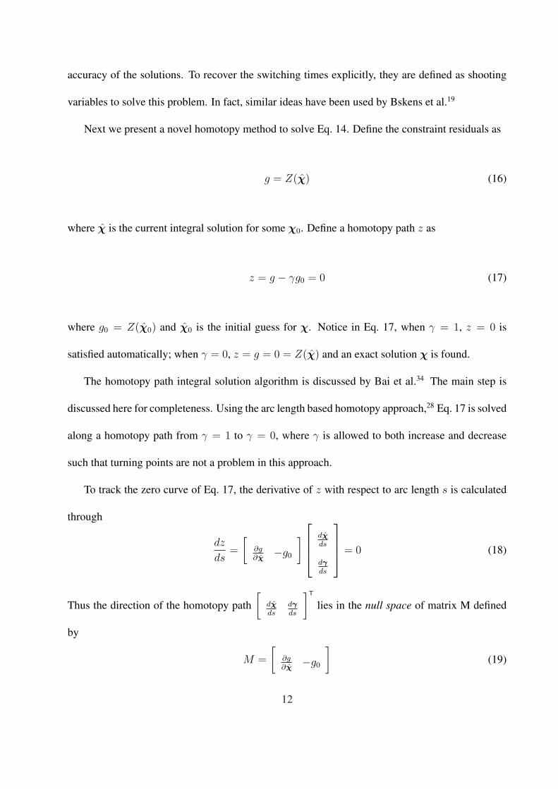
accuracy of the solutions. To recover the switching times explicitly, they are defined as shooting

variables to solve this problem. In fact, similar ideas have been used by Bskens et al.19

Next we present a novel homotopy method to solve Eq. 14. Define the constraint residuals as

g = Z(χ) (16)

where χ is the current integral solution for some χ0. Define a homotopy path z as

z = g − γg0 = 0 (17)

where g0 = Z(χ0) and χ0 is the initial guess for χ. Notice in Eq. 17, when γ = 1, z = 0 is

satisfied automatically; when γ = 0, z = g = 0 = Z(χ) and an exact solution χ is found.

The homotopy path integral solution algorithm is discussed by Bai et al.34 The main step is

discussed here for completeness. Using the arc length based homotopy approach,28 Eq. 17 is solved

along a homotopy path from γ = 1 to γ = 0, where γ is allowed to both increase and decrease

such that turning points are not a problem in this approach.

To track the zero curve of Eq. 17, the derivative of z with respect to arc length s is calculated

through

dz

ds=

[∂g∂χ

−g0

]

dχds

dγds

= 0 (18)

Thus the direction of the homotopy path[

dχds

dγds

]T

lies in the null space of matrix M defined

by

M =

[∂g∂χ

−g0

](19)

12

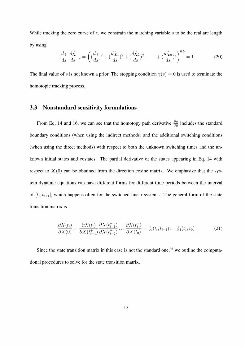
While tracking the zero curve of z, we constrain the marching variable s to be the real arc length

by using

‖dγ

ds,dχ

ds‖2 =

((dγ

ds)2 + (

dχ1

ds)2 + (

dχ2

ds)2 + . . . + (

dχn

ds)2

)0.5

= 1 (20)

The final value of s is not known a prior. The stopping condition γ(s) = 0 is used to terminate the

homotopic tracking process.

3.3 Nonstandard sensitivity formulations

From Eq. 14 and 16, we can see that the homotopy path derivative ∂g∂χ

includes the standard

boundary conditions (when using the indirect methods) and the additional switching conditions

(when using the direct methods) with respect to both the unknown switching times and the un-

known initial states and costates. The partial derivative of the states appearing in Eq. 14 with

respect to X(0) can be obtained from the direction cosine matrix. We emphasize that the sys-

tem dynamic equations can have different forms for different time periods between the interval

of [ti, ti+1], which happens often for the switched linear systems. The general form of the state

transition matrix is

∂X(ti)

∂X(0)=

∂X(ti)

∂X(t+i−1)

∂X(t−i−1)

∂X(t+i−2). . .

∂X(t−1 )

∂X(t0)= φi(ti, ti−1) . . . φ1(t1, t0) (21)

Since the state transition matrix in this case is not the standard one,36 we outline the computa-

tional procedures to solve for the state transition matrix.

13

We integrate Eq. 13 to obtain

X(t) = X(0) +

∫ t

0

h(X,u, t)dt (22)

where X(0) consists of both the known and the unknown initial states and co-states.

Taking the derivatives of Eq. 22 with respect to X(0)

∂X(t)

∂X(0)= I +

∫ t

0

(∂h

∂X(t)

∂X(t)

∂X(0)+

∂h

∂u2

∂u2

∂X(t)

∂X(t)

∂X(0)

)dt (23)

we obtain the differential equations for the state transition matrix by taking the time derivative,

yielding

d

dt(∂X(t)/∂X(0)) =

(∂h

∂X(t)+

∂h

∂u2

∂u2

∂X(t)

)∂X

∂X0

(24)

Notice since u1 has already been taken care of by the bang-bang form, the partial derivatives

we calculate here only involve the non-bang-bang controls. Additionally, in Eq. 24, we assume the

optimal control is an implicit function of the states. The numerical expression for ∂u2/∂X(t) is

obtained from the Hamiltonian. The stationary condition provides the form for the optimal control

as

Hu =∂H

∂u2

= 0 (25)

where H is the Hamiltonian function. Taking the derivative of Eq. 25 with respect to X(t), we

obtain

∂Hu

∂X(t)=

∂Hu

∂X(t)+

∂Hu

∂u2

∂u2

∂X(t)= 0 (26)

14

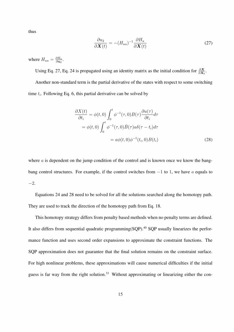
thus

∂u2

∂X(t)= −(Huu)

−1 ∂Hu

∂X(t)(27)

where Huu = ∂Hu

∂u2.

Using Eq. 27, Eq. 24 is propagated using an identity matrix as the initial condition for ∂X∂X0

.

Another non-standard term is the partial derivative of the states with respect to some switching

time ti. Following Eq. 6, this partial derivative can be solved by

∂X(t)

∂ti= φ(t, 0)

∫ t

0

φ−1(τ, 0)B(τ)∂u(τ)

∂tidτ

= φ(t, 0)

∫ t

0

φ−1(τ, 0)B(τ)aδ(τ − ti)dτ

= aφ(t, 0)φ−1(ti, 0)B(ti) (28)

where a is dependent on the jump condition of the control and is known once we know the bang-

bang control structures. For example, if the control switches from −1 to 1, we have a equals to

−2.

Equations 24 and 28 need to be solved for all the solutions searched along the homotopy path.

They are used to track the direction of the homotopy path from Eq. 18.

This homotopy strategy differs from penalty based methods when no penalty terms are defined.

It also differs from sequential quadratic programming(SQP).40 SQP usually linearizes the perfor-

mance function and uses second order expansions to approximate the constraint functions. The

SQP approximation does not guarantee that the final solution remains on the constraint surface.

For high nonlinear problems, these approximations will cause numerical difficulties if the initial

guess is far way from the right solution.33 Without approximating or linearizing either the con-

15

straints or performance function, the proposed algorithm achieves its robustness by enforcing the

satisfaction of the dynamic equation constraints along the homotopy path. In this way, we enlarge

the convergence domain of the initial guess for the two-point boundary value problems.

4 An Orbit Rendezvous Example Problem

This example is a simplified version of a subproblem from the 4th Global Trajectory Opti-

misation Competition.41 The problem is to design an planar optimal trajectory starting from one

asteroid and intercepting with another asteroid within a fixed time. We require the spacecraft on a

circular orbit at both the initial time and the final intercepting time.

4.1 Mathematical Formulations

The spacecraft is assumed to be a point mass with a variable mass m and only the gravity force

from the Sun is considered. The position of the spacecraft in a solar-centric polar coordinate is

(r, θ) as shown in Fig. 1, where r is the distance of the spacecraft to the Sun and θ is the phase

angle with respect to some inertial axis. u is the velocity along the radial direction and v is the

velocity along the local horizontal direction. The angle between the thrust direction and the local

horizontal is the control variable represented by β.

16

uv

x

y

r

θ

T

β

Sun

S/C

0

Fig. 1 Frame, State and Control Definition

The dynamic equations for the spacecraft are

r = u (29)

θ = v/r (30)

u = v2/r − µ/r2 + T/m sin β (31)

v = −uv/r + T/m cos β (32)

where the thrust magnitude is bounded

0 ≤ T ≤ 0.135N (33)

The mass equation is

m = − T

g0Isp

(34)

The spacecraft has a constant specific impulse Isp as 3000sec. The initial mass is 1500kg and

17

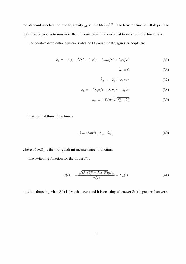
the standard acceleration due to gravity g0 is 9.80665m/s2. The transfer time is 240days. The

optimization goal is to minimize the fuel cost, which is equivalent to maximize the final mass.

The co-state differential equations obtained through Pontryagin’s principle are

λr = −λu(−v2/r2 + 2/r3)− λvuv/r2 + λθv/r2 (35)

λθ = 0 (36)

λu = −λr + λvv/r (37)

λv = −2λuv/r + λvu/r − λθ/r (38)

λm = −T/m2√

λ2u + λ2

v (39)

The optimal thrust direction is

β = atan2(−λu,−λv) (40)

where atan2() is the four-quadrant inverse tangent function.

The switching function for the thrust T is

S(t) = −√

(λu(t)2 + λv(t)2)gIsp

m(t)− λm(t) (41)

thus it is thrusting when S(t) is less than zero and it is coasting whenever S(t) is greater than zero.

18

The two-point boundary conditions are

r(0) = 1 (42)

θ(0) = 0 (43)

v(0) = 0 (44)

m(0) = 1 (45)

r(tf ) = 1.05242919219003 (46)

θ(tf ) = 3.99191781862267 (47)

u(f) = 0 (48)

v(f) = 0.97477314754443 (49)

λm(f) = −1 (50)

where all the distance variables have been non-dimensionalized by 1AU = 1.495978706910000×

1011m; all the variables involving time have been non-dimensionalized by 1TU = 5.022642890912782×

106sec; the mass is non-dimensionalized by the initial mass 1500kg. All these non-dimensionalizations

lead to that the maximum thrust magnitude is 0.01517685201253; the maximum mass flow rate is

m = 0.01536501116359; the transfer time is 4.12850374800020TU .

4.2 Approximate Solutions from Pseudospectral Method

Although the homotopy method is robust when compared with the standard gradient based

methods, for bang-bang type of problems, decent control structures, and switching times are re-

quired for its successes. We obtain these information from a pseudospectral method. The code is

19

implemented in MATLAB. SNOPT.7 is the nonlinear programming solver that provides the major

feasibility tolerance, minor feasibility tolerance, and major optimality tolerance as 1e− 6.

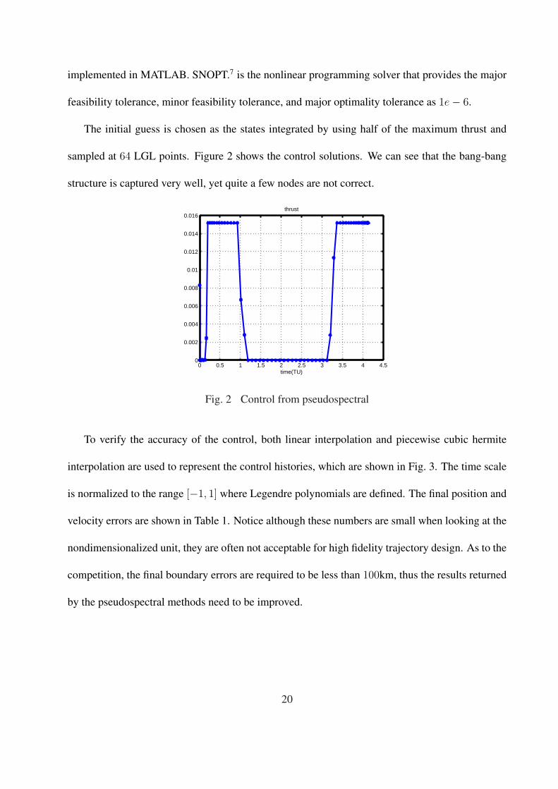
The initial guess is chosen as the states integrated by using half of the maximum thrust and

sampled at 64 LGL points. Figure 2 shows the control solutions. We can see that the bang-bang

structure is captured very well, yet quite a few nodes are not correct.

0 0.5 1 1.5 2 2.5 3 3.5 4 4.50

0.002

0.004

0.006

0.008

0.01

0.012

0.014

0.016

time(TU)

thrust

Fig. 2 Control from pseudospectral

To verify the accuracy of the control, both linear interpolation and piecewise cubic hermite

interpolation are used to represent the control histories, which are shown in Fig. 3. The time scale

is normalized to the range [−1, 1] where Legendre polynomials are defined. The final position and

velocity errors are shown in Table 1. Notice although these numbers are small when looking at the

nondimensionalized unit, they are often not acceptable for high fidelity trajectory design. As to the

competition, the final boundary errors are required to be less than 100km, thus the results returned

by the pseudospectral methods need to be improved.

20

−1 −0.5 0 0.5 10

0.002

0.004

0.006

0.008

0.01

0.012

0.014

0.016

Normalized time

Thr

ust

Interpolated thrust with PS solution

PSlinearPiecewise Cubic Hermite

Fig. 3 Interpolated thrust with PS solution

Final Errors Linear interpolation Piecewise Cubic hermite Interpolation4r(AU)

4u(AU/TU)4v(AU/TU)4θ(rad)

0.12583599381699× 10−3

0.18681358039823× 10−3

0.37652130891286× 10−3

0.01071562338772× 10−3

0.11586689900422× 10−3

0.16111720421912× 10−3

0.38315737654437× 10−3

−0.04031962569595× 10−3

Table 1 Final Errors

4.3 Optimal Solution from Homotopy Method

Using the initial co-states obtained from the pseudospectral methods and the approximate

switching times as the initial guess for the homotopy method, we find accurate switching times

and initial co-states with the optimal trajectory. The initial co-states and switching times from the

pseudospectral methods and the homotopy solutions are listed in Table 2.

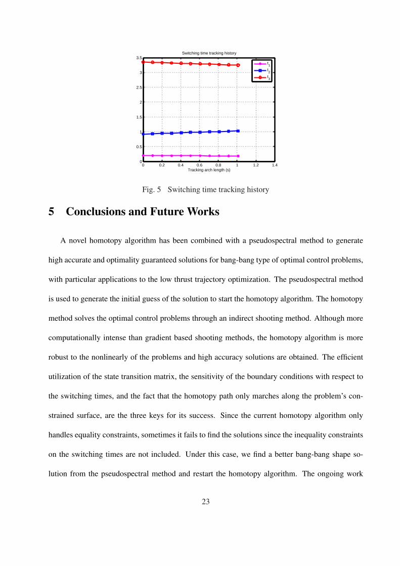
The homotopy tracking histories are shown in Figs. 4 and 5, which is the path the homotopy

method marches along, starting with the solutions from the psedospectral method and ending at

the accurate optimal solutions. The optimal trajectory is shown in Fig. 6. The optimal state history

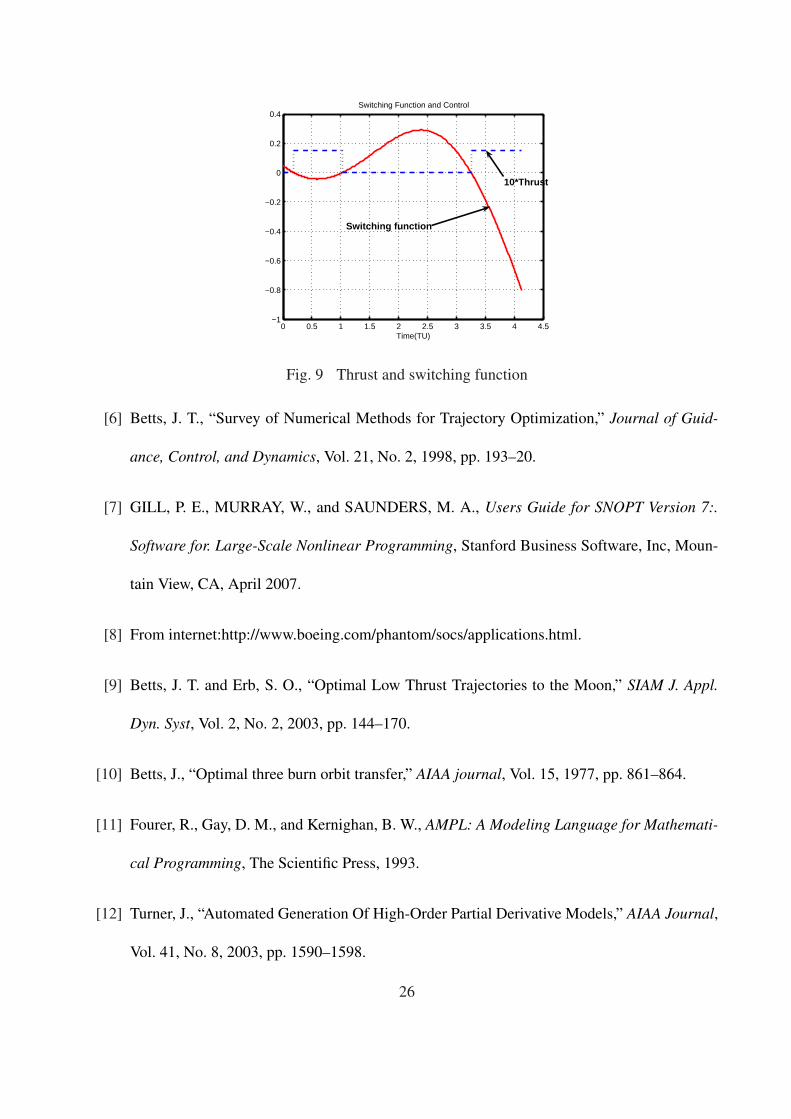
is shown in Fig. 7 with the mass history in Fig. 8. The switching function and the thrust magni-

tude are shown in Fig. 9, which clearly shows that the obtained control satisfies the Pontryagin’s

21

Initial conditions and switching times pseudospectral homotopyλr(t0)λφ(t0)λu(t0)λv(t0)λm(t0)

t1t2t3

−0.47908295213219−0.166437088621670.33263137092118−0.85778071767051−0.97740428340329

0.20.9253.35

−0.48433902798013−0.167544268854000.31568214760216−0.87711007733394−0.968202235384110.184361026651541.028309909099803.25065284139823

Table 2 Initial co-states and switching times

principles. Notice for illustration purpose the thrust magnitude has been multiplied by ten. The

final errors, which include the boundary condition in Eqs. from 46 to 50 and the three switching

functions S(ti) = 0, i = 1, 2, 3 in Eq. 41, are less than 10−11. The final mass is 0.9735, which

means 2.645547298022% mass was consumed during the transfer.

0 0.2 0.4 0.6 0.8 1 1.2 1.4−1

−0.8

−0.6

−0.4

−0.2

0

0.2

0.4

Tracking arch length (s)

Initial lambda tracking history

λr(0)

λφ(0)

λu(0)

λv(0)

λm

(0)

Fig. 4 Co-state tracking history

22

0 0.2 0.4 0.6 0.8 1 1.2 1.40

0.5

1

1.5

2

2.5

3

3.5

Tracking arch length (s)

Switching time tracking history

t1

t2

t3

Fig. 5 Switching time tracking history

5 Conclusions and Future Works

A novel homotopy algorithm has been combined with a pseudospectral method to generate

high accurate and optimality guaranteed solutions for bang-bang type of optimal control problems,

with particular applications to the low thrust trajectory optimization. The pseudospectral method

is used to generate the initial guess of the solution to start the homotopy algorithm. The homotopy

method solves the optimal control problems through an indirect shooting method. Although more

computationally intense than gradient based shooting methods, the homotopy algorithm is more

robust to the nonlinearly of the problems and high accuracy solutions are obtained. The efficient

utilization of the state transition matrix, the sensitivity of the boundary conditions with respect to

the switching times, and the fact that the homotopy path only marches along the problem’s con-

strained surface, are the three keys for its success. Since the current homotopy algorithm only

handles equality constraints, sometimes it fails to find the solutions since the inequality constraints

on the switching times are not included. Under this case, we find a better bang-bang shape so-

lution from the pseudospectral method and restart the homotopy algorithm. The ongoing work

23

0.5

1

1.5

30

210

60

240

90

270

120

300

150

330

180 0

Transfer orbit and thrust directionon

off

on

off

thrust direction

thrust direction

Fig. 6 Orbit transfer trajectory

includes extending the homotopy method to solve inequality constrained problems, thus both or-

dering switching times and state constrained problems are expected to be solved.

References

[1] Frank L. Lewis, V. L. S., Optimal control, Wiley-Interscience, 1995, pp.134, 284.

[2] D.BILIMORIA, K. and WIE, B., “Time-Optimal Three-Axis Reorientation of a Rigid Space-

craft,” Journal of Guidance, Control, and Dynamics, Vol. 16, No. 3, 1993, pp. 446–452.

[3] Bai, X. and Junkins, J. L., “New Results for Time-Optimal Three-Axis Reorientation of

a Rigid Spacecraft,” Journal of Guidance, Control, and Dynamics, Vol. 32, No. 4, 2009,

pp. 1071–1076.

24

0 2 4 60.95

1

1.05

1.1r

Time(TU)

r

0 2 4 60

1

2

3

4φ

Time(TU)

φ

0 2 4 6−0.01

0

0.01

0.02

0.03u

Time(TU)

u

0 2 4 60.96

0.98

1

1.02

1.04v

Time(TU)

v

offonoffon

Fig. 7 Optimal state history

0 0.5 1 1.5 2 2.5 3 3.5 4 4.50.97

0.975

0.98

0.985

0.99

0.995

1

1.005mass

Time(sec)

m(n

on−

dim

ensi

onal

ized

)

Fig. 8 Optimal mass history

[4] Oberle, H. J. and Taubert, K., “Existence and Multiple Solutions of the Minimum-Fuel Orbit

Transfer Problem,” Journal of Optimization Theory and Applications, Vol. 95, No. 2, Nov.

1997, pp. 243–262.

[5] Bertrand, R. and Epenoy, R., “New smoothing techniques for solving bang-bang optimal con-

trol problems - numerical results and statistical interpretation,” Optimal Control Applications

and Methods, Vol. 23, No. 4, 2002, pp. 171 – 197.

25

0 0.5 1 1.5 2 2.5 3 3.5 4 4.5−1

−0.8

−0.6

−0.4

−0.2

0

0.2

0.4Switching Function and Control

Time(TU)

10*Thrust

Switching function

Fig. 9 Thrust and switching function

[6] Betts, J. T., “Survey of Numerical Methods for Trajectory Optimization,” Journal of Guid-

ance, Control, and Dynamics, Vol. 21, No. 2, 1998, pp. 193–20.

[7] GILL, P. E., MURRAY, W., and SAUNDERS, M. A., Users Guide for SNOPT Version 7:.

Software for. Large-Scale Nonlinear Programming, Stanford Business Software, Inc, Moun-

tain View, CA, April 2007.

[8] From internet:http://www.boeing.com/phantom/socs/applications.html.

[9] Betts, J. T. and Erb, S. O., “Optimal Low Thrust Trajectories to the Moon,” SIAM J. Appl.

Dyn. Syst, Vol. 2, No. 2, 2003, pp. 144–170.

[10] Betts, J., “Optimal three burn orbit transfer,” AIAA journal, Vol. 15, 1977, pp. 861–864.

[11] Fourer, R., Gay, D. M., and Kernighan, B. W., AMPL: A Modeling Language for Mathemati-

cal Programming, The Scientific Press, 1993.

[12] Turner, J., “Automated Generation Of High-Order Partial Derivative Models,” AIAA Journal,

Vol. 41, No. 8, 2003, pp. 1590–1598.

26

[13] Bai, X., Turner, J. D., and Junkins, J. L., “Automatic Differentiation Based Dynamic Model

for a Mobile Stewart Platform,” 7th International Conference On Dynamics and Control of

Systems and Structures in Space, London, England, July 2006.

[14] Nah, R. S., Vadali, S. R., and Braden, E., “Fuel-Optimal, Low-Thrust, Three-Dimensional

EarthMars Trajectories,” Journal of Guidance, Control, and Dynamics, Vol. 24, No. 6, 2001,

pp. 1100–1107.

[15] Bulirsch, R. and R.Callies, “Optimal trajectories for a multiple rendezvous mission to aster-

oids,” Acta Astronautica, Vol. 26, No. 8-10, 1992, pp. 587–587.

[16] Ranieri, C. and Ocampo, C., “Optimization of Roundtrip, Time-Constrained, Finite Burn

Trajectories via an Indirect Method,” Journal of Guidance, Control, and Dynamics, Vol. 28,

No. 2, 2005, pp. 0731–5090.

[17] Jr., A., “Optimal control-1950 to 1985,” Control Systems Magazine, IEEE, Vol. 16, No. 3,

1966, pp. 26–33.

[18] Bryson, A. E. and Yu-Chi, H., Applied Optimal Control: Optimization, Estimation, and Con-

trol, Hemisphere Publishing Corporation, Washington D.C, 1975.

[19] C.Bskens, Pesch, H. J., and Winderl, S., Online Optimization of Large Scale Systems: State

of the Art, chap. Real-time solutions of bang-bang and singular optimal control problems,

Springer, 2001, pp. 129–142.

[20] Maurer, H. and Osmolovskii, N. P., “Second Order Sufficient Conditions for Time-Optimal

Bang-Bang Control,” SIAM Journal on Control and Optimization, Vol. 42, No. 6, 2004,

pp. 2239–2263.

27

[21] Stryk, O. V. and Bulirsch, R., “Direct and indirect methods for trajectory optimization,” An-

nals of Operations Research, Vol. 37, No. 1, 1992, pp. 357–373.

[22] Maurer, H. and Pesch, H. J., “Direct optimization methods for solving a complex state-

constrained optimal control problem in microeconomics,” Applied Mathematics and Com-

putation, Vol. 204, No. 2, 2008, pp. 568–579.

[23] Canuto, C., M.Y.Hussaini, A.Quarteroni, and Zang, T., SPECTRAL METHODS IN FLUID

DYNAMICS (Springer Series in Computational Physics), Springer-verlag, 1988.

[24] Fahroo, F. and Ross, I. M., “Direct Trajectory Optimization by a Chebyshev Pseudospec-

tral Method,” Journal of Guidance, Control, and Dynamics, Vol. 25, No. 1, Jan.-Feb. 2002,

pp. 160–166.

[25] Fahroo, F. and Ross, I. M., “A spectral patching method for direct trajectory optimization,”

Journal of the Astronautical Sciences, Vol. 48, No. 2/3, 2000, pp. 269–286.

[26] Ross, I., Gong, Q., and Sekhavat, P., “Low-thrust, high-accuracy trajectory optimization,”

Journal of Guidance Control and Dynamics,, Vol. 30, No. 4, 2007, pp. 921–933.

[27] Q Gong, F Fahroo, I. R., “Spectral Algorithm for Pseudospectral Methods in Optimal Con-

trol,” Journal of Guidance Control and Dynamics, Vol. 31, No. 3, 2008, pp. 460–471.

[28] Chow, S.-N., Mallet-Paret, J., and Yorke, J. A., “Finding Zeroes of Maps: Homotopy Methods

That are Constructive With Probability One,” Mathematics of Computation, Vol. 32, No. 143,

Jul. 1978, pp. 887–889.

28

[29] Watson, L. T. and Haftka, R. T., “Modern homotopy methods in optimization,” Computer

Methods in Applied Mechanics and Engineering, Vol. 74, No. 3, September 1989, pp. 289 –

305.

[30] Morgan, A., Solving Polynomial Systems Using Continuation for Engineering and Scientific

Problems, Prentice Hall, Englewood Cliffs, New Jersey, April 1987.

[31] Bulirsch, R., Montrone, F., and Pesch, H. J., “Abort landing in the presence of windshear as

a minimax optimal control problem, part 1: Necessary conditions,” Journal of Optimization

Theory and Applications, Vol. 70, No. 1, July 1991, pp. 1–23.

[32] Bulirsch, R., Montrone, F., and Pesch, H. J., “Abort landing in the presence of windshear

as a minimax optimal control problem, part 2: Multiple shooting and homotopy,” Journal of

Optimization Theory and Applications, Vol. 70, No. 2, August 1991, pp. 223–254.

[33] Bai, X., Turner, J. D., and Junkins, J. L., “A Robust Homotopy Method for Equality Con-

strained Nonlinear Optimization,” 2008 12th AIAA/ISSMO Multidisciplinary Analysis and

Optimization Conference.

[34] Bai, X., Turner, J. D., and Junkins, J. L., “Optimal Thrust Design of a Mission to Apophis

Based on a Homotopy Method,” 2009 AAS/AIAA Spaceflight Mechanics Meeting, February

9-12, 2009, Savannah, Georgia, Feb. 2009.

[35] Garg, D., Patterson, M., Darby, C., Francolin, C., Hager, W., and Ra, A., “Direct Trajec-

tory Optimization and Costate Estimation of Finite-Horizon and Infinite-Horizon Optimal

Control Problems Using a Radau Pseudospectral Method,” Computational Optimization and

Applications, conditionally accepted for publication.

29

[36] Schaub, H. and Junkins, J. L., Analytical Mechanics of Space Systems, AIAA Education

Series, AIAA, Reston, VA, 2003, pp. 492-495.

[37] Egerstedt, M., Wardi, Y., and Delmotte, F., “Optimal control of switching times in switched

dynamical systems,” Decision and Control, 2003. Proceedings. 42nd IEEE Conference on,

Vol. 3, Dec 2003, pp. 2138– 2143.

[38] Xu, X. and Antsaklis, P., “Optimal control of switched systems based on parameterization of

the switching instants,” Automatic Control, IEEE Transactions on, Vol. 49, No. 1, Jan. 2004,

pp. 2– 16.

[39] Sun, Z. and Geb, S., “Analysis and synthesis of switched linear control systemsstar, open,”

Automatica, Vol. 41, No. 2, Feb. 2005, pp. 181–195.

[40] Nocedal, J. and Wright, S. J., Numerical Optimization, Springer, Verlag New York, April

2000, pp. 425.

[41] From internet: http://cct.cnes.fr/cct02/gtoc4/index.htm.

30