Bandwidth selection for estimating the two-point

correlation function of a spatial point pattern using

AMSE

Ji Meng Loh⇤

Dept of Mathematical Sciences

New Jersey Institute of Technology

Newark, New Jersey

Woncheol Jang†

Dept of Statistics

Seoul National University

Republic of Korea

March 21, 2014

Abstract

We introduce an asymptotic mean squared error (AMSE) approach to obtain closed-

form expressions of the adaptive optimal bandwidths for estimating the two-point cor-

relation function of a homogeneous spatial point pattern. The two-point correlation

function is one of several second-order measures of clustering of a point pattern and is

commonly used in astronomy where cosmologists have found a relationship between the

clustering of galaxies and the evolution of the universe. The AMSE approach is adapted

from an AMISE approach that is well-known in density estimation and our approach

provides a simple and quick method for optimal bandwidth selection for estimating

the two-point correlation function. Using optimal bandwidths for estimation will allow

more information about clustering to be extracted from the data. Results from numer-

ical studies suggest that the mean squared error of estimates obtained using AMSE

optimal bandwidths is competitive with those obtained using more computationally

intensive methods and is close to the empirical optimal bandwidths. We illustrate its

use in an application to a galaxy cluster catalog from the Sloan Digital Sky Survey.

Keywords: Bandwidth selection, second-order clustering, spatial point patterns, two-point correlation function

⇤Email: loh@njit.edu; Tel: 973-596-2949; Fax: 973-596-5591

†Email: wcjang@stats.snu.ac.kr

1

1 Introduction

In the analysis of spatial point patterns, it is often of interest to quantify the clustering ofthe points, i.e. the degree of clumpiness or regularity observed in the point pattern. Theclustering in the points often reflect the underlying process driving the placement of points.For example, the clustering of galaxies is believed to be due to the e↵ects of gravitation overan extremely long period of time. In ecological studies, the presence of regularity of trees ina forest may be due to the competition for soil resources.

In this paper, we consider the problem of finding an optimal bin size or bandwidth forestimating the two-point correlation function (2PCF) of an observed spatial point pattern.The two-point correlation function is a measure of second-order clustering and is routinelyused by astronomers to quantify the clustering of astronomical objects such as galaxies andquasi-stellar objects (Martınez and Saar, 2001). We focus on estimators which astronomershave developed that empirically account for boundary e↵ects, and use an asymptotic meansquared error (AMSE) approach to find optimal bandwidths for these estimators.

Although third and higher-order measures of clustering have been studied in astronomyand in other areas (Kim et al., 2011; Szapudi et al., 2001), second-order measures andespecially the 2PCF in astronomy are still the norm. Our method for finding the optimalbandwidth can be extended to apply to third and higher-order measures.

Second-order measures relate to the behavior of point pairs and is quantified by thedistributions of inter-point distances. Various measures have been used to measure second-order clustering of a spatial point pattern, e.g. the second-order product density ⇢

(2), Ripley’sK function, the pair correlation function g and the two-point correlation function ⇠. Eachquantity is a function of the inter-point distance r.

Intuitively, the second-order product density ⇢

(2) is related to the probability of finding apair of points, one in each of two small volumes dS

1

and dS

2

separated by distance r. Moreformally, if N(dS) represents the number of points in the volume dS,

⇢

(2)(r) = lim|dS|!0

N(dS)N(dS + r)

|dS|2,

where |dS| represents the volume of dS and dS+ r is dS translated by r. If the spatial pointprocess is isotropic, ⇢(2)(r) = ⇢

(2)(r), where r = |r|. The various second-order measures arerelated to each other as follows:

K(r) =

Zr

0

4⇡u2g(u) du in R3

,

g(r) = ⇢

(2)(r)/�2, and

⇠(r) = g(r)� 1.

The 2PCF is popular in astronomy because the cosmological models describing the evo-lution of the universe link the two-point correlation of astronomical objects such as galaxiesto cosmological parameters that control the universe’s evolution. A well-known success story

2

in cosmological modeling is the prediction of a bump in the 2PCF due to an event called“recombination” that was subsequently observed in the empirical 2PCF estimated from data(Ryden, 2003).

Estimating quantities such as the two-point correlation function from data requires count-ing pairs of points that are distance r apart. This requires specifying a bandwidth, the focusof this paper. The e↵ects of the observation region boundary also has to be taken into ac-count, since the neighborhood of a point close to the boundary is not fully observed. Thereare several analytical methods for dealing with edge e↵ects (Baddeley et al., 1993; Illian etal, 2008). Probably due to the irregular boundaries of the observation regions, astronomerstend to use numerical methods. Specifically, suppose we use D and R to represent the dataand a randomly generated set of points, with N

D

and N

R

number of points respectively.Define

DD = DD(r0

) =X

x2D

X

y2D1{r

0

� h |x� y| r

0

+ h}/ND

(ND

� 1),

DR = DR(r0

) =X

x2D

X

y2R1{r

0

� h |x� y| r

0

+ h}/ND

N

R

,

RR = RR(r0

) =X

x2R

X

y2R1{r

0

� h |x� y| r

0

+ h}/NR

(NR

� 1).

Then the Landy-Szalay estimator (Landy and Szalay, 1993) of the two-point correlationfunction is given by

⇠

LS

(r0

) = (DD � 2DR +RR)/RR.

There are other estimators of ⇠, such as the Hamilton, the Peebles and the Hewitt estimators.See Kerscher et al. (2000) for a review of these estimators. The Landy-Szalay and Hamiltonestimators are generally considered to be the better estimators, with smaller standard errors,with the Landy-Szalay estimator being more commonly used. These two estimators aresimilar to the estimators constructed by Loh et al. (2001) for the purpose of reducing standarderrors.

We propose using an approach similar to the asymptotic mean integrated squared error(AMISE) in the density estimation literature to obtain optimal bandwidths for the estimationof the 2PCF. We describe the AMISE method for density estimation in the subsectionbelow. In Section 2 we describe the application of the AMISE approach to the 2PCF,removing the integration from the original AMISE approach to obtain an AMSE methodthat allows us to select adaptive bandwidths depending on r. Section 3 describes the resultsof a simulation study comparing the bandwidths obtained using AMSE with empiricallyoptimal bandwidths. In Section 4 we apply the AMSE method to a Sloan Digital SkySurvey dataset of galaxy clusters. Section 5 concludes this paper.

3

1.1 Bandwidth selection for density estimation

In this section, we give an overview of bandwidth selection in density estimation. Suppse wehave n independent identically distributed random variables, X

1

, . . . , X

n

with an unknowndensity function f . The kernel density estimator of f(x) is given by

f

h

(x) =1

nh

nX

i=1

K

✓x�X

i

h

◆

where h is the bandwidth and K is a kernel function. We assume that K satisfiesZ

K(x)dx = 1,

ZxK(x) = 0, and

Zx

2

K(x) < 1.

The most common criterion for measuring the global accuracy of f , an estimator of f , is themean integrated square error (MISE):

MISE(f) = E

Z ⇣f(x)� f(x)

⌘2

dx

It is well known that the choice of kernel K is not crucial in density estimation whereasthe choice of bandwidth h is important. Various data-driven bandwidth selectors have beenproposed and most of them are motivated by di↵erent ways of minimizing the MISE. To seehow the choice of the bandwidth make influence on the MISE, one considers the approxima-tion of MISE with leading variance and bias terms:

MISE(f) =

Z ⇣E(f(x))� f(x)

⌘2

dx+

ZV ar(f(x))dx

=1

nh

ZK(t)2dt+

1

4h

4

µ

2

(K)2Z

f

00(x)2dx+ o

✓1

nh

+ h

4

◆,

where µ

2

(K) =Rt

2

K

2(t)dt.See Silverman (1986) for details. We can then define the asymptotic mean integrated

square error as follows:

AMISE(f) =1

nh

ZK(t)2dt+

1

4h

4

µ

2

(K)2Z

f

00(x)2dx,

ignoring the smaller order terms. With simple algebra, the optimal bandwidth that minimizesthe AMISE is given by

h

opt

=

✓R(K)

µ

2

(K)2R(f 00)n

◆1/5

where R(g) =Rg

2(x)dx. However, R(f 00) is unknown so we cannot calculate the aboveoptimal bandwidth in practice. A easy way to address this issue is to assume f to be a

4

specific density function. For example, in the normal reference rule, f is assumed to be thenormal density with variance �

2, and one can easily show that h

normal

= 1.06�n�1/5. Amore sophisticated way of estimating R(f 00) is to use the kernel density estimator. This,however, requires the expectation of the 4th derivative of f . This latter quantity can also beobtained using a kernel estimator, but its optimal bandwidth depends on the expectation ofthe 6th derivative of f . Usually, at this point, one applies the normal reference rule to selectthe optimal bandwidth for the kernel estimator of the 6th derivative of f .

Other popular bandwidth selectors include least squares cross-validation and likelihoodcross-validation. See Silverman (1986). However, the aforementioned plug-in bandwidthselector provides a closed form of the optimal bandwidth and these plug-in methods have anadvantage in computation over cross-validation based bandwidth selectors.

2 AMSE for the 2PCF

To estimate the 2PCF, we need a bandwidth h for computing DD,DR and RR. Often anad-hoc approach is used to select the optimal bandwidth. For example, Stoyan et al. (1995)proposed using the bandwidth h = c�

�1/d for the Epanechnikov kernel where d representsthe dimension of the observational area and c is a constant. For planar point pattern of50-300 points, they suggested c 2 (0.1, 0.2) with c = .15 being a common choice (Guan,2007). Instead of the Epanechnikov kernel, Stoyan (2006) recommended the box kernel, butdid not provide guidelines on how to select the optimal bandwidth with the box kernel. For3 dimensions, Pons-Borderia et al . (1999) recommended c = 0.05 and 0.1 for clustered andPoisson point processes respectively. Their approach is similar to the normal reference rule.While these approaches provide a closed-form expression for the optimal bandwidth, theoptimal bandwidth is derived based on the strong assumption on the underlying process.Therefore, we develop a simple bandwidth selection method which is similar to the plug-in bandwidth in density estimation so the selection of bandwidth can be less sensitive tothe assumption on the underlying process. Furthermore, our approach allows for adaptivebandwidth selection depending of r.

Let the kernel Kh

(t) be defined as a boxcar kernel: K

h

(t) = 1

2h

1{|t| h}, so thatDD = DD(r

0

) = 2hP

x

Py

K

h

(r0

� |x � y|) and similarly for DR and RR. Note thatRh

�h

K

h

(t) dt = 1. We then have

E(RR) = 2h

Z

A

Z

A

K

h

(r0

� |x� y|)�2R

dy dx

= 2h�2R

Z

A

Z 1

0

Z

⇥

K

h

(r0

� r)1A

{x+ (r, ✓)} r2d✓ dr dx,

= 2h�2R

Z

A

Z 1

0

K

h

(r0

� r)

Z

⇥

1A

{x+ (r, ✓)} r2d✓�dr dx,

= 2h�2R

Z

A

Z 1

0

K

h

(r0

� r)C(r) dr dx,

5

where in the second line above we have expressed y in spherical coordinates: y = x+ (r, ✓),with r 2 (0,1), ✓ 2 ⇥, and included the indicator function 1

A

{x + (r, ✓)} to ensure thaty 2 A. The quantity C(r) represents the edge e↵ect due to the boundary of A. It is equalto 4⇡r2 in three dimensions if x is more than r away from the boundary of A. For small h,r ⇡ r

0

and therefore C(r) ⇡ C(r0

) ⌘ C

0

. Replacing C(r) with C(r0

) above helps simplifythe expression:

E(RR) ⇡ 2h�2R

C

0

Z

A

dx

Z 1

0

K

h

(r0

� r) dr

= 2h�2R

|A|C0

, if r0

> h.

sinceR10

K

h

(r0

� r) dr =Rr

0

+h

r

0

�h

1{|r0

� r| h}/2h dr = 1 if r0

> h. Similarly, we have

E(DR) ⇡ 2h�D

�

R

|A|C0

,

E(DD) ⇡ 2h�2D

|A|C0

Z 1

0

K

h

(r0

� r)g(r) dr.

Note that if we set �

R

= �

D

, then E(DR) = E(RR), and the di↵erence between E(DD)and E(RR) is the presence of g(r) in the integrand. Therefore,

E[⇠LS

(r0

)] ⇡ 1

h

Z 1

0

K

✓r

0

� r

h

◆g(r) dr � 1, when r

0

> h,

where K(t) = 1

2

1{|t| 1}. The approximation above is obtained by taking the ratio of theexpected values, and noting that K

h

(t) = K(t/h)/h. Using a Taylor expansion of g(r) aboutr

0

, we find that the bias is

Bias(⇠LS

(r0

)) = E[⇠LS

(r0

)]� 1� ⇠(r0

)

=1

h

Z 1

0

K

✓r

0

� r

h

◆g(r) dr � 1� ⇠(r

0

)

=

Z 1

�r

0

/h

K(t)g(r0

+ th) dt� 1� ⇠(r0

) (Here t ⌘ (r � r

0

)/h)

⇡Z 1

�r

0

/h

K(t)

g(r

0

) + g

0(r0

)th+1

2g

00(r0

)t2h2�dt� 1� ⇠(r

0

)

= g(r0

)

Z 1

�r

0

/h

K(t) dt� 1� ⇠(r0

) + g

0(r0

)h

Z 1

�r

0

/h

tK(t) dt

+g

00(r0

)h2

2

Z 1

�r

0

/h

t

2

K(t) dt

=g

00(r0

)h2

2µ

2

(K) + o(h2) because

ZK(t) dt = 1,

ZtK(t) dt = 0 when r

0

> h

=g

00(r0

)h2

6+ o(h2).

6

In the last line above, we have written µ

2

(K) =R1�r

0

/h

t

2

K(t) dt = 1/3 if r0

> h.

Landy and Szalay (1993) derived an approximation for the variance of ⇠LS

. Specifically,

Var[⇠LS

(r0

)] = E[1 + ⇠

LS

(r0

)]2/(2h�2|A|C0

),

so that its leading term is g(r0

)2/(2h�2|A|C0

). Together with the bias, we have,

MSE(r0

) ⇡ [g00(r0

)]2

36h

4 +

✓1

h

⇥ g(r0

)2

2�2|A|C0

◆. (1)

We can obtain an optimal bandwidth from (1) by minimizing the expression with respect toh. Di↵erentiating (1) with respect to h we get the optimal bandwidth as

h

opt

(r0

) =

9g(r

0

)2

2�2|A|C0

g

00(r0

)2

�1/5

. (2)

Note that the expression depends on the unknown function g = 1 + ⇠ as well as its secondderviative. A simple procedure to get an optimal bandwidth from the above is to use aplug-in approach and assume a specific form for g (or ⇠).

We choose as the expression for g that of the Thomas modified process (Thomas, 1949).The Thomas process is a Neyman-Scott process where the points are the o↵spring of parentpoints. The parent points follow a homogeneous Poisson process with intensity �. Eachparent point has a Poisson number of o↵spring points (with mean number µ) that, for themodifed Thomas process are distributed about the parents according to a Gaussian densitywith standard deviation �. For the modified Thomas process,

g(r) = 1 +µ

4⇡��2e

�r

2

/4�

2

.

Using the above expression for g, we get an optimal bandwidth h

opt

given by

h

opt

(r0

) =

0

@ 72�8

�

2|A|C0

"4⇡��2 + µe

�r

2

/4�

2

µ(r2 � 2�2)e�r

2

/4�

2

#2

1

A1/5

. (3)

Alternatively, in astronomy, a commonly used functional form for the 2PCF is the power-law model, ⇠(r) = (r/s

0

)�� , which is known to fit a wide range of empirical data well. If weuse this model in the expression (2), we get

h

opt

(r0

) =

9

2�2|A|C0

�

2(� + 1)2

1 +

✓r

0

s

0

◆�

�2

r

4

0

!1/5

. (4)

We note that this optimal bandwidth is an adaptive bandwidth, i.e. a value is obtainedfor every value of r

0

. This is in contrast to the plug-in optimal bandwidths in kernel density

7

estimation. We also note that since h is usually relatively small, the assumption of r0

> h

is not very restrictive.In an actual application, instead of �2|A|C

0

, we can replace it with the average of RR/2hevaluated over a range of values of h, where RR is as defined before, using �

R

= �

D

. Valuesof � and s

0

can be obtained from fits of the power-law model to the data.

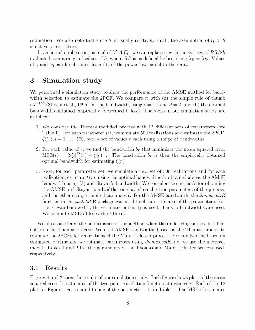
3 Simulation study

We performed a simulation study to show the performance of the AMSE method for band-width selection to estimate the 2PCF. We compare it with (a) the simple rule of thumbc�

�1/d (Stoyan et al., 1995) for the bandwidth, using c = .15 and d = 2, and (b) the optimalbandwidths obtained empirically (described below). The steps in our simulation study areas follows:

1. We consider the Thomas modified process with 12 di↵erent sets of parameters (seeTable 1). For each parameter set, we simulate 500 realizations and estimate the 2PCF,⇠

i

b

(r), i = 1, . . . , 500, over a set of values r each using a range of bandwidths.

2. For each value of r, we find the bandwidth b

r

that minimizes the mean squared errorMSE(r) =

Pi

[⇠ib

(r) � ⇠(r)]2. The bandwidth b

r

is then the empirically obtainedoptimal bandwidth for estimating ⇠(r).

3. Next, for each parameter set, we simulate a new set of 500 realizations and for eachrealization, estimate ⇠(r), using the optimal bandwidths b

r

obtained above, the AMSEbandwidth using (3) and Stoyan’s bandwidth. We consider two methods for obtainingthe AMSE and Stoyan bandwidths, one based on the true parameters of the process,and the other using estimated parameters. For the AMSE bandwidth, the thomas.estK

function in the spatstat R package was used to obtain estimates of the parameters. Forthe Stoyan bandwidth, the estimated intensity is used. Thus, 5 bandwidths are used.We compute MSE(r) for each of them.

We also considered the performance of the method when the underlying process is di↵er-ent from the Thomas process. We used AMSE bandwidths based on the Thomas process toestimate the 2PCFs for realizations of the Matern cluster process. For bandwidths based onestimated parameters, we estimate parameters using thomas.estK, i.e. we use the incorrectmodel. Tables 1 and 2 list the parameters of the Thomas and Matern cluster process used,respectively.

3.1 Results

Figures 1 and 2 show the results of our simulation study. Each figure shows plots of the meansquared error for estimates of the two-point correlation function at distance r. Each of the 12plots in Figure 1 correspond to one of the parameter sets in Table 1. The MSE of estimates

8

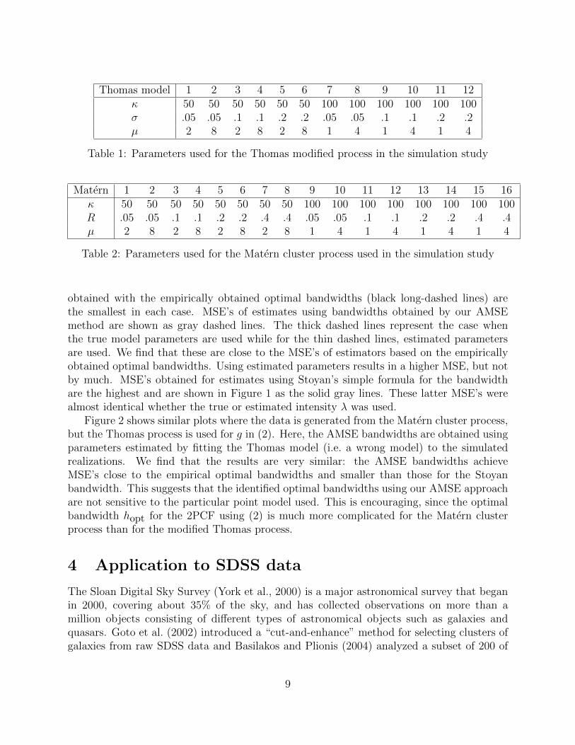
Thomas model 1 2 3 4 5 6 7 8 9 10 11 12 50 50 50 50 50 50 100 100 100 100 100 100� .05 .05 .1 .1 .2 .2 .05 .05 .1 .1 .2 .2µ 2 8 2 8 2 8 1 4 1 4 1 4

Table 1: Parameters used for the Thomas modified process in the simulation study

Matern 1 2 3 4 5 6 7 8 9 10 11 12 13 14 15 16 50 50 50 50 50 50 50 50 100 100 100 100 100 100 100 100R .05 .05 .1 .1 .2 .2 .4 .4 .05 .05 .1 .1 .2 .2 .4 .4µ 2 8 2 8 2 8 2 8 1 4 1 4 1 4 1 4

Table 2: Parameters used for the Matern cluster process used in the simulation study

obtained with the empirically obtained optimal bandwidths (black long-dashed lines) arethe smallest in each case. MSE’s of estimates using bandwidths obtained by our AMSEmethod are shown as gray dashed lines. The thick dashed lines represent the case whenthe true model parameters are used while for the thin dashed lines, estimated parametersare used. We find that these are close to the MSE’s of estimators based on the empiricallyobtained optimal bandwidths. Using estimated parameters results in a higher MSE, but notby much. MSE’s obtained for estimates using Stoyan’s simple formula for the bandwidthare the highest and are shown in Figure 1 as the solid gray lines. These latter MSE’s werealmost identical whether the true or estimated intensity � was used.

Figure 2 shows similar plots where the data is generated from the Matern cluster process,but the Thomas process is used for g in (2). Here, the AMSE bandwidths are obtained usingparameters estimated by fitting the Thomas model (i.e. a wrong model) to the simulatedrealizations. We find that the results are very similar: the AMSE bandwidths achieveMSE’s close to the empirical optimal bandwidths and smaller than those for the Stoyanbandwidth. This suggests that the identified optimal bandwidths using our AMSE approachare not sensitive to the particular point model used. This is encouraging, since the optimalbandwidth h

opt

for the 2PCF using (2) is much more complicated for the Matern clusterprocess than for the modified Thomas process.

4 Application to SDSS data

The Sloan Digital Sky Survey (York et al., 2000) is a major astronomical survey that beganin 2000, covering about 35% of the sky, and has collected observations on more than amillion objects consisting of di↵erent types of astronomical objects such as galaxies andquasars. Goto et al. (2002) introduced a “cut-and-enhance” method for selecting clusters ofgalaxies from raw SDSS data and Basilakos and Plionis (2004) analyzed a subset of 200 of

9

0.00 0.05 0.10 0.15 0.20

02

46

8

r

MSE

(κ, σ, µ) = (50, 0.05, 2)

0.00 0.05 0.10 0.15 0.20

02

46

8

r

MSE

(κ, σ, µ) = (50, 0.05, 8)

0.00 0.05 0.10 0.15 0.20

01

23

4

r

MSE

(κ, σ, µ) = (50, 0.1, 2)

0.00 0.05 0.10 0.15 0.20

01

23

4

r

MSE

(κ, σ, µ) = (50, 0.1, 8)

0.00 0.05 0.10 0.15 0.20

0.0

0.5

1.0

1.5

2.0

r

MSE

(κ, σ, µ) = (50, 0.2, 2)

0.00 0.05 0.10 0.15 0.20

0.0

0.5

1.0

1.5

2.0

r

MSE

(κ, σ, µ) = (50, 0.2, 8)

0.00 0.05 0.10 0.15 0.20

02

46

8

r

MSE

(κ, σ, µ) = (100, 0.05, 1)

0.00 0.05 0.10 0.15 0.20

02

46

8

r

MSE

(κ, σ, µ) = (100, 0.05, 4)

0.00 0.05 0.10 0.15 0.20

01

23

4

r

MSE

(κ, σ, µ) = (100, 0.1, 1)

0.00 0.05 0.10 0.15 0.20

01

23

4

r

MSE

(κ, σ, µ) = (100, 0.1, 4)

0.00 0.05 0.10 0.15 0.20

0.0

0.5

1.0

1.5

2.0

r

MSE

(κ, σ, µ) = (100, 0.2, 1)

0.00 0.05 0.10 0.15 0.20

0.0

0.5

1.0

1.5

2.0

r

MSE

(κ, σ, µ) = (100, 0.2, 4)

Figure 1: Plots showing the mean squared error (MSE) of estimates of the two-point cor-relation function of the Thomas process using empirically obtained optimal bandwidths(black long-dashed lines), bandwidths obtained using our AMSE method (gray thick andthin dashed lines) and using the Stoyan’s rule of thumb (gray solid lines). The thick andthin dashed lines represent MSE’s from using, respectively, the true and estimated modelparameters in the AMSE method.

10

0.00 0.10 0.20

05

1015

r

MSE

(κ, σ, µ) = (50, 0.05, 2)

0.00 0.10 0.200

510

15

r

MSE

(κ, σ, µ) = (50, 0.05, 8)

0.00 0.10 0.20

02

46

8

r

MSE

(κ, σ, µ) = (50, 0.1, 2)

0.00 0.10 0.20

02

46

8

r

MSE

(κ, σ, µ) = (50, 0.1, 8)

0.00 0.10 0.20

01

23

4

r

MSE

(κ, σ, µ) = (50, 0.2, 2)

0.00 0.10 0.20

01

23

4

r

MSE

(κ, σ, µ) = (50, 0.2, 8)

0.00 0.10 0.200.

00.

51.

01.

52.

0

r

MSE

(κ, σ, µ) = (50, 0.4, 2)

0.00 0.10 0.20

0.0

0.5

1.0

1.5

2.0

r

MSE

(κ, σ, µ) = (50, 0.4, 8)

0.00 0.10 0.20

05

1015

r

MSE

(κ, σ, µ) = (100, 0.05, 1)

0.00 0.10 0.20

05

1015

r

MSE

(κ, σ, µ) = (100, 0.05, 4)

0.00 0.10 0.20

02

46

8

r

MSE

(κ, σ, µ) = (100, 0.1, 1)

0.00 0.10 0.200

24

68

r

MSE

(κ, σ, µ) = (100, 0.1, 4)

0.00 0.10 0.20

01

23

4

r

MSE

(κ, σ, µ) = (100, 0.2, 1)

0.00 0.10 0.20

01

23

4

r

MSE

(κ, σ, µ) = (100, 0.2, 4)

0.00 0.10 0.20

0.0

0.5

1.0

1.5

2.0

r

MSE

(κ, σ, µ) = (100, 0.4, 1)

0.00 0.10 0.20

0.0

0.5

1.0

1.5

2.0

r

MSE

(κ, σ, µ) = (100, 0.4, 4)

Figure 2: Plots showing the mean squared error (MSE) of estimates of the two-point corre-lation function of the Matern cluster process using empirically obtained optimal bandwidths(black long-dashed lines), bandwidths obtained using our AMSE method based on the in-correct Thomas model (gray dashed lines) and using the Stoyan’s rule of thumb (gray solidlines).

11

these galaxies. Loh and Jang (2010) also used this data set in conjunction with a bootstrapbandwidth selection procedure. More detailed description of the galaxy catalog, such as theregions in the sky in which they are located, can be found in Goto et al. (2002); Basilakosand Plionis (2004); Loh and Jang (2010).

In this section, we obtain results from applying our AMSE bandwidth selection procedureto this galaxy catalog. Specifically, we use (4) to obtain adaptive bandwidths for obtainingthe Landy-Szalay estimator of ⇠. We considered distances from 5 to 100 h

�1 Mpc and usedvalues of 20.7 and 1.6 for s

0

and � respectively. These values were obtained as estimates ofs

0

and � by Basilakos and Plionis (2004) through fitting a power-law model for ⇠.Figure 3 shows the bandwidths found from (4) and from the bootstrap bandwidth pro-

cedure of Loh and Jang (2010), and estimates of ⇠ using these bandwidths. We find thatthe adaptive bootstrap bandwidths using the method in Loh and Jang (2010) (black dots inFigure 3) are more variable, but also tend to be larger, producing much smoother estimatesof ⇠. The overall bootstrap bandwidth, represented in the left plot of Figure 3 by a horizontaldashed line, is a single value applying to all values of r. Its value of 7 is on the lower end ofthe range of the adaptive bootstrap bandwidths and produces a more jagged curve for ⇠.

The AMSE bandwidths fall between these two. The bandwidths increase as r increase,with smaller bandwidths than both the overall and adaptive bootstrap bandwidths forr < 40h�1 Mpc. For r > 40h�1 Mpc, the AMSE bandwidths become larger than theoverall bootstrap bandwidth, having values comparable to those of the adaptive bootstrapbandwidths. This behavior in the values of the AMSE bandwidths is reflected in the result-ing estimate of ⇠, shown on the log scale in the right-hand plot of Figure 3. The estimateis slightly more jagged for r < 40h�1 Mpc, but still comparable with the estimate obtainedwith the overall bootstrap bandwidth. Its smoothness for r > 40h�1 Mpc lies betweenthe two bootstrap bandwidth versions, closer to the estimate obtained using the adaptivebootstrap bandwidths.

Hence, we find that the procedure performs reasonably well. Recall that the AMSEbandwidths are obtained using the closed-form expression in (4) and thus is very easy toobtain, unlike the bootstrap optimal bandwidths which require a more computationallyexpensive bootstrap procedure.

5 Conclusion

We introduced the use of the AMSE approach, common in density estimation, as a method forobtaining optimal bandwidths for estimating the 2PCF, which is widely used in astronomy.Loh and Jang (2010) introduced an optimal bandwidth selection method that uses bootstrap.However, this latter method is computationally intensive, and with the very large data sizesnow common in astronomy, a quick way to obtain optimal bandwidths for estimating the2PCF will be very useful. The AMSE method introduced here provides a closed form solutionthat is easily computed. It is not much more complicated than Stoyan’s rule of thumb forthe bandwidth, yet our simulation studies suggest that it can produce estimates of the 2PCFwith substantially smaller mean square errors. Also, the method naturally yields optimal

12

5 20 40 60 80 1000

10

20

30

40

r

bw

●●●●●

●●●●

●

●

●●●●●●

●

●●●

●●

●

●●

●●

●

●●●●●●●●●●●●

●

●●

●●

●●

●●●●

●

●●

●

●

●●●

●●

●●●●

●●●●●●●

●●●

●●

●

●●●

●●●●●●

●

●●●●●

●●

●

●●●

●●●●●

●●●●●●●●●●●

●●●●●●●●●●

●●●●●●●●●●

●●●●●●●●

●●●●●●●●●

●●●●●●●●

●●●●●●●

●●●●●●●●

●●●●●●●

●●●●●●●

●●●●●●●

●●●

5 10 20 50 100

0

2

4

6

8

10

r

ξ

AMSE bwadaptive bootstrap bwoverall bootstrap bw

Figure 3: Plots showing, on the left, the overall (dashed line) and adaptive bandwidths(clear dots) obtained by a bootstrap bandwidth procedure (Loh and Jang, 2010) and adaptivebandwidths using AMSE (solid dots), and, on the right, estimates of the two-point correlationfunction using these bandwidths, on the log scale.

adaptive bandwidths, i.e. optimal bandwidths are obtained for each distance r of interest.This can be useful in astronomy applications since the range of distances considered areoften very large.

References

Baddeley, A., Moyeed, R., Howard, C. and Boyde, A. (1993). Analysis of a three-dimensionalpoint pattern with replication. Journal of the Royal Statistical Society, Series C, 42, 641–668.

Basilakos, S. and Plionis, M. (2004). Modeling the two-point correlation function of galaxyclusters in the Sloan Digital Sky Survey. Monthly Notices of the Royal Astronomical Soci-

ety, 349, 882-888.

Goto, T., Sekiguchi, M., Nichol, R.C., Bahcall, N.A., Kim, R.S.J., Annis, J., Ivezic, Z.,Brinkmann, J., Hennessy, G.S., Szokoly, G.P. and Tucker, D.L. (2002). The cut-an-enhancemethod: selecting clusters of galaxies from the Sloan Digital Sky Survey commissioningdata. Astronomical Journal, 123, 1807–1825.

Guan, Y. (2007). A least squares cross-validation bandwidth selection approach in pair cor-relation measures. Statistics and Probability Letters, 77, 1722–1729.

Illian ,J., Penttinen, A., Stoyan, H. and Stoyan, D. (2008). Statistical analysis and modelling

of spatial point patterns. New York: John Wiley and Sons.

13

Kerscher, M., Szapudi, I., and Szalay, A. S. (2000). A comparison of estimators for the twopoint correlation function. Astrophysical Journal Letters, 535, 13–16.

Kim, S., Nowozin, S., Kohli, P., and Yoo, C. D. (2011). Higher-order correlation clustering forimage segmentation,” In Advances in Neural Information Processing Systems, 24, 1530–1538.

Landy, S. D. and Szalay, A. S. (1993). Bias and variance of angular correlation functions.Astrophysical Journal, 412, 64–71.

Loh, J. M. and Jang, W. (2008). Estimating a cosmological mass bias parameter with boot-strap bandwidth selection. Journal of the Royal Statistical Society, Series C, 59, 761–779.

Loh, J. K., Quashnock, J. M. and Stein, M. L. (2001). A Measurement of the Three-dimensional Clustering of C IV Absorption-Line Systems on Scales of 51000 h

�1 Mpc.Astrophysical Journal, 560, 606–616.

Martınez, V. J. and Saar, E. (2001). Statistics of the galaxy distribution. New York: Chapman& Hall/CRC Press.

Pons-Borderia, M.-J., Marinez, V. J., Stoyan, D., Stoyan, H. and Saar, E. (1999). Comparingestimators of the galaxy correlation function. Astrophysical Journal, 523, 480–491

Ryden, B. (2003). Introduction to Cosmology. Boston: Addison-Wesley.

Silverman, B. W. (1986). Density Estimation for Statistics and Data Analysis. New York:Chapman & Hall/CRC Press.

Stoyan, D. (2006). Fundamentals of point process statistics. In Case Studies in Spatial Point

Process Modeling (eds Baddeley, A., Gregori, P., Mateu, J., Stoica, R. and Stoyan, D.),3–22. New York: Springer.

Stoyan, D., Kendall, W. S. and Mecke, J. (1995). Stochastic Geometry and Its Applications,2nd edition, New York: Wiley

Szapudi, I., Postman, M., Lauer, T. R. and Oegerle, William (2001). Observational con-straints on higher order clustering up to z ' 1 Astrophysical Journal , 548, 114–126.

Thomas, M. (1949). A generalisation of Poisson’s binomial limit for use in ecology.Biometrika, 36, 18–25.

York, D.G., Adelman, J., Anderson, J.E., et al. (2000). The Sloan Digital Sky Survey:Technical summary. Astronomical Journal, 120, 1579–1587.

14