
BAND Manual - Software for Chemistry & Materials · The periodic DFT program BAND can be used for...
306
BAND Manual Amsterdam Modeling Suite 2019.3 www.scm.com Nov 08, 2019
Transcript of BAND Manual - Software for Chemistry & Materials · The periodic DFT program BAND can be used for...

BAND ManualAmsterdam Modeling Suite 2019.3
www.scm.com
Nov 08, 2019

CONTENTS
1 General 11.1 Introduction . . . . . . . . . . . . . . . . . . . . . . . . . . . . . . . . . . . . . . . . . . . . . . . 11.2 Feature List . . . . . . . . . . . . . . . . . . . . . . . . . . . . . . . . . . . . . . . . . . . . . . . . 1
1.2.1 Model Hamiltonians . . . . . . . . . . . . . . . . . . . . . . . . . . . . . . . . . . . . . . 11.2.2 Structure and Reactivity . . . . . . . . . . . . . . . . . . . . . . . . . . . . . . . . . . . . 21.2.3 Spectroscopy and Properties . . . . . . . . . . . . . . . . . . . . . . . . . . . . . . . . . . 21.2.4 Charge transport . . . . . . . . . . . . . . . . . . . . . . . . . . . . . . . . . . . . . . . . 21.2.5 Analysis . . . . . . . . . . . . . . . . . . . . . . . . . . . . . . . . . . . . . . . . . . . . . 2
1.3 What’s new in Band 2019 . . . . . . . . . . . . . . . . . . . . . . . . . . . . . . . . . . . . . . . . 31.3.1 New features in Band 2019.3 . . . . . . . . . . . . . . . . . . . . . . . . . . . . . . . . . . 31.3.2 New features in Band 2019.1 . . . . . . . . . . . . . . . . . . . . . . . . . . . . . . . . . . 3
1.4 Input . . . . . . . . . . . . . . . . . . . . . . . . . . . . . . . . . . . . . . . . . . . . . . . . . . . 31.4.1 General remarks on input structure and parsing . . . . . . . . . . . . . . . . . . . . . . . . 41.4.2 Keys . . . . . . . . . . . . . . . . . . . . . . . . . . . . . . . . . . . . . . . . . . . . . . . 51.4.3 Blocks . . . . . . . . . . . . . . . . . . . . . . . . . . . . . . . . . . . . . . . . . . . . . . 61.4.4 Units . . . . . . . . . . . . . . . . . . . . . . . . . . . . . . . . . . . . . . . . . . . . . . 7
2 Exploring the PES with AMS 92.1 Input Geometry . . . . . . . . . . . . . . . . . . . . . . . . . . . . . . . . . . . . . . . . . . . . . . 92.2 Single Point . . . . . . . . . . . . . . . . . . . . . . . . . . . . . . . . . . . . . . . . . . . . . . . 92.3 Geometry Optimization . . . . . . . . . . . . . . . . . . . . . . . . . . . . . . . . . . . . . . . . . 92.4 Transition State Search . . . . . . . . . . . . . . . . . . . . . . . . . . . . . . . . . . . . . . . . . . 92.5 Linear Transit and other PES Scan . . . . . . . . . . . . . . . . . . . . . . . . . . . . . . . . . . . . 92.6 Molecular Dynamics . . . . . . . . . . . . . . . . . . . . . . . . . . . . . . . . . . . . . . . . . . . 102.7 Nuclear Gradients and Stress Tensor . . . . . . . . . . . . . . . . . . . . . . . . . . . . . . . . . . . 10
3 Model Hamiltonians 113.1 Density Functional (XC) . . . . . . . . . . . . . . . . . . . . . . . . . . . . . . . . . . . . . . . . . 11
3.1.1 LDA/GGA/metaGGA . . . . . . . . . . . . . . . . . . . . . . . . . . . . . . . . . . . . . . 123.1.2 Dispersion Correction . . . . . . . . . . . . . . . . . . . . . . . . . . . . . . . . . . . . . . 143.1.3 Model Potentials . . . . . . . . . . . . . . . . . . . . . . . . . . . . . . . . . . . . . . . . 163.1.4 Non-Collinear Approach . . . . . . . . . . . . . . . . . . . . . . . . . . . . . . . . . . . . 173.1.5 LibXC Library Integration . . . . . . . . . . . . . . . . . . . . . . . . . . . . . . . . . . . 173.1.6 Range-separated hybrid functionals . . . . . . . . . . . . . . . . . . . . . . . . . . . . . . 183.1.7 Defaults and special cases . . . . . . . . . . . . . . . . . . . . . . . . . . . . . . . . . . . 193.1.8 GGA+U . . . . . . . . . . . . . . . . . . . . . . . . . . . . . . . . . . . . . . . . . . . . . 193.1.9 OEP . . . . . . . . . . . . . . . . . . . . . . . . . . . . . . . . . . . . . . . . . . . . . . . 203.1.10 DFT-1/2 . . . . . . . . . . . . . . . . . . . . . . . . . . . . . . . . . . . . . . . . . . . . . 21
3.2 Relativistic Effects and Spin . . . . . . . . . . . . . . . . . . . . . . . . . . . . . . . . . . . . . . . 243.2.1 Spin polarization . . . . . . . . . . . . . . . . . . . . . . . . . . . . . . . . . . . . . . . . 24
i
3.2.2 Relativistic Effects . . . . . . . . . . . . . . . . . . . . . . . . . . . . . . . . . . . . . . . 243.3 Solvation . . . . . . . . . . . . . . . . . . . . . . . . . . . . . . . . . . . . . . . . . . . . . . . . . 25
3.3.1 COSMO: Conductor like Screening Model and the Solvation-key . . . . . . . . . . . . . . . 253.3.2 Additional keys for periodic systems . . . . . . . . . . . . . . . . . . . . . . . . . . . . . . 303.3.3 SM12: Solvation Model 12 . . . . . . . . . . . . . . . . . . . . . . . . . . . . . . . . . . . 31
Input . . . . . . . . . . . . . . . . . . . . . . . . . . . . . . . . . . . . . . . . . . . . . . . 313.4 Electric and Magnetic Fields . . . . . . . . . . . . . . . . . . . . . . . . . . . . . . . . . . . . . . . 37
3.4.1 Electric Field . . . . . . . . . . . . . . . . . . . . . . . . . . . . . . . . . . . . . . . . . . 373.4.2 Magnetic Field . . . . . . . . . . . . . . . . . . . . . . . . . . . . . . . . . . . . . . . . . 373.4.3 Atoim-wise fuzzy potential . . . . . . . . . . . . . . . . . . . . . . . . . . . . . . . . . . . 39
3.5 Nuclear Model . . . . . . . . . . . . . . . . . . . . . . . . . . . . . . . . . . . . . . . . . . . . . . 39
4 Accuracy and Efficiency 414.1 Basis set . . . . . . . . . . . . . . . . . . . . . . . . . . . . . . . . . . . . . . . . . . . . . . . . . 41
4.1.1 Basis input block . . . . . . . . . . . . . . . . . . . . . . . . . . . . . . . . . . . . . . . . 424.1.2 Which basis set should I use? . . . . . . . . . . . . . . . . . . . . . . . . . . . . . . . . . . 424.1.3 Available Basis Sets . . . . . . . . . . . . . . . . . . . . . . . . . . . . . . . . . . . . . . . 454.1.4 More Basis input options . . . . . . . . . . . . . . . . . . . . . . . . . . . . . . . . . . . . 464.1.5 Confinement of basis functions . . . . . . . . . . . . . . . . . . . . . . . . . . . . . . . . . 464.1.6 Manually specifying AtomTypes (expert option) . . . . . . . . . . . . . . . . . . . . . . . . 474.1.7 Basis Set Superposition Error (BSSE) . . . . . . . . . . . . . . . . . . . . . . . . . . . . . 49
4.2 K-Space . . . . . . . . . . . . . . . . . . . . . . . . . . . . . . . . . . . . . . . . . . . . . . . . . 494.2.1 KSpace input block . . . . . . . . . . . . . . . . . . . . . . . . . . . . . . . . . . . . . . . 49
Regular K-Space grid . . . . . . . . . . . . . . . . . . . . . . . . . . . . . . . . . . . . . . . 50Symmetric K-Space grid (tetrahedron method) . . . . . . . . . . . . . . . . . . . . . . . . . 51
4.2.2 Recommendations for k-space . . . . . . . . . . . . . . . . . . . . . . . . . . . . . . . . . 524.3 Numerical Integration . . . . . . . . . . . . . . . . . . . . . . . . . . . . . . . . . . . . . . . . . . 52
4.3.1 Becke Grid . . . . . . . . . . . . . . . . . . . . . . . . . . . . . . . . . . . . . . . . . . . 524.3.2 Radial grid of NAOs . . . . . . . . . . . . . . . . . . . . . . . . . . . . . . . . . . . . . . 554.3.3 Voronoi grid (deprecated) . . . . . . . . . . . . . . . . . . . . . . . . . . . . . . . . . . . . 55
4.4 Density Fitting . . . . . . . . . . . . . . . . . . . . . . . . . . . . . . . . . . . . . . . . . . . . . . 564.4.1 Zlm Fit . . . . . . . . . . . . . . . . . . . . . . . . . . . . . . . . . . . . . . . . . . . . . 56
Expert options . . . . . . . . . . . . . . . . . . . . . . . . . . . . . . . . . . . . . . . . . . 574.4.2 STO Fit (Deprecated) . . . . . . . . . . . . . . . . . . . . . . . . . . . . . . . . . . . . . . 59
4.5 Hartree–Fock RI . . . . . . . . . . . . . . . . . . . . . . . . . . . . . . . . . . . . . . . . . . . . . 594.6 Self Consistent Field (SCF) . . . . . . . . . . . . . . . . . . . . . . . . . . . . . . . . . . . . . . . 60
4.6.1 SCF block . . . . . . . . . . . . . . . . . . . . . . . . . . . . . . . . . . . . . . . . . . . . 604.6.2 Convergence . . . . . . . . . . . . . . . . . . . . . . . . . . . . . . . . . . . . . . . . . . 624.6.3 DIIS . . . . . . . . . . . . . . . . . . . . . . . . . . . . . . . . . . . . . . . . . . . . . . . 634.6.4 Multi secant . . . . . . . . . . . . . . . . . . . . . . . . . . . . . . . . . . . . . . . . . . . 654.6.5 DIRIS . . . . . . . . . . . . . . . . . . . . . . . . . . . . . . . . . . . . . . . . . . . . . . 66
4.7 More Technical Settings . . . . . . . . . . . . . . . . . . . . . . . . . . . . . . . . . . . . . . . . . 664.7.1 Linear Scaling . . . . . . . . . . . . . . . . . . . . . . . . . . . . . . . . . . . . . . . . . . 664.7.2 Dependency . . . . . . . . . . . . . . . . . . . . . . . . . . . . . . . . . . . . . . . . . . . 674.7.3 Screening . . . . . . . . . . . . . . . . . . . . . . . . . . . . . . . . . . . . . . . . . . . . 674.7.4 Direct (on the fly) calculation of basis and fit . . . . . . . . . . . . . . . . . . . . . . . . . 684.7.5 Fermi energy search . . . . . . . . . . . . . . . . . . . . . . . . . . . . . . . . . . . . . . . 694.7.6 Block size . . . . . . . . . . . . . . . . . . . . . . . . . . . . . . . . . . . . . . . . . . . . 69
5 Spectroscopy and Properties 715.1 Frequencies and Phonons . . . . . . . . . . . . . . . . . . . . . . . . . . . . . . . . . . . . . . . . 715.2 Elastic Tensor . . . . . . . . . . . . . . . . . . . . . . . . . . . . . . . . . . . . . . . . . . . . . . 715.3 Optical Properties: Time-Dependent Current DFT . . . . . . . . . . . . . . . . . . . . . . . . . . . 71
5.3.1 Insulators, semiconductors and metals . . . . . . . . . . . . . . . . . . . . . . . . . . . . . 71
ii

5.3.2 Frequency dependent kernel . . . . . . . . . . . . . . . . . . . . . . . . . . . . . . . . . . 725.3.3 EELS . . . . . . . . . . . . . . . . . . . . . . . . . . . . . . . . . . . . . . . . . . . . . . 725.3.4 Input Options . . . . . . . . . . . . . . . . . . . . . . . . . . . . . . . . . . . . . . . . . . 73
NewResponse . . . . . . . . . . . . . . . . . . . . . . . . . . . . . . . . . . . . . . . . . . . 73OldResponse . . . . . . . . . . . . . . . . . . . . . . . . . . . . . . . . . . . . . . . . . . . 77
5.4 ESR/EPR . . . . . . . . . . . . . . . . . . . . . . . . . . . . . . . . . . . . . . . . . . . . . . . . . 795.5 Nuclear Quadrupole Interaction (EFG) . . . . . . . . . . . . . . . . . . . . . . . . . . . . . . . . . 815.6 NMR . . . . . . . . . . . . . . . . . . . . . . . . . . . . . . . . . . . . . . . . . . . . . . . . . . . 825.7 Effective Mass . . . . . . . . . . . . . . . . . . . . . . . . . . . . . . . . . . . . . . . . . . . . . . 825.8 Properties at Nuclei . . . . . . . . . . . . . . . . . . . . . . . . . . . . . . . . . . . . . . . . . . . 835.9 X-Ray Form Factors . . . . . . . . . . . . . . . . . . . . . . . . . . . . . . . . . . . . . . . . . . . 84
6 Analysis 856.1 Density of States (DOS) . . . . . . . . . . . . . . . . . . . . . . . . . . . . . . . . . . . . . . . . . 85
6.1.1 Gross populations . . . . . . . . . . . . . . . . . . . . . . . . . . . . . . . . . . . . . . . . 876.1.2 Overlap populations . . . . . . . . . . . . . . . . . . . . . . . . . . . . . . . . . . . . . . . 88
6.2 Band Structure . . . . . . . . . . . . . . . . . . . . . . . . . . . . . . . . . . . . . . . . . . . . . . 886.2.1 User-defined path in the Brillouin zone . . . . . . . . . . . . . . . . . . . . . . . . . . . . . 906.2.2 Definition of the Fat Bands . . . . . . . . . . . . . . . . . . . . . . . . . . . . . . . . . . . 916.2.3 Band Gap . . . . . . . . . . . . . . . . . . . . . . . . . . . . . . . . . . . . . . . . . . . . 91
6.3 Charges . . . . . . . . . . . . . . . . . . . . . . . . . . . . . . . . . . . . . . . . . . . . . . . . . . 916.3.1 Default Atomic Charge Analysis . . . . . . . . . . . . . . . . . . . . . . . . . . . . . . . . 916.3.2 Bader Analysis (AIM) . . . . . . . . . . . . . . . . . . . . . . . . . . . . . . . . . . . . . 92
6.4 Fragments . . . . . . . . . . . . . . . . . . . . . . . . . . . . . . . . . . . . . . . . . . . . . . . . 946.5 Energy Decomposition Analysis . . . . . . . . . . . . . . . . . . . . . . . . . . . . . . . . . . . . . 95
6.5.1 Periodic Energy Decomposition Analysis (PEDA) . . . . . . . . . . . . . . . . . . . . . . . 956.5.2 Periodic Energy Decomposition Analysis and natural orbitals of chemical valency (PEDA-
NOCV) . . . . . . . . . . . . . . . . . . . . . . . . . . . . . . . . . . . . . . . . . . . . . 966.6 3D field visualization with BAND . . . . . . . . . . . . . . . . . . . . . . . . . . . . . . . . . . . . 97
7 Electronic Transport (NEGF) 1037.1 Transport with NEGF in a nutshell . . . . . . . . . . . . . . . . . . . . . . . . . . . . . . . . . . . . 103
7.1.1 Self consistency . . . . . . . . . . . . . . . . . . . . . . . . . . . . . . . . . . . . . . . . . 1057.1.2 Contour integral . . . . . . . . . . . . . . . . . . . . . . . . . . . . . . . . . . . . . . . . . 1057.1.3 Gate potential . . . . . . . . . . . . . . . . . . . . . . . . . . . . . . . . . . . . . . . . . . 1067.1.4 Bias potential . . . . . . . . . . . . . . . . . . . . . . . . . . . . . . . . . . . . . . . . . . 106
7.2 Workflow . . . . . . . . . . . . . . . . . . . . . . . . . . . . . . . . . . . . . . . . . . . . . . . . . 1067.3 Input options . . . . . . . . . . . . . . . . . . . . . . . . . . . . . . . . . . . . . . . . . . . . . . . 107
7.3.1 SGF Input options . . . . . . . . . . . . . . . . . . . . . . . . . . . . . . . . . . . . . . . . 1077.3.2 NEGF Input options (no bias) . . . . . . . . . . . . . . . . . . . . . . . . . . . . . . . . . 1077.3.3 NEGF Input options (with bias) . . . . . . . . . . . . . . . . . . . . . . . . . . . . . . . . 1107.3.4 NEGF Input options (alignment) . . . . . . . . . . . . . . . . . . . . . . . . . . . . . . . . 112
7.4 Troubleshooting . . . . . . . . . . . . . . . . . . . . . . . . . . . . . . . . . . . . . . . . . . . . . 1137.5 Miscellaneous remarks on BAND-NEGF . . . . . . . . . . . . . . . . . . . . . . . . . . . . . . . . 113
7.5.1 Store tight-binding Hamiltonian . . . . . . . . . . . . . . . . . . . . . . . . . . . . . . . . 113
8 Expert Options 1158.1 Restarts . . . . . . . . . . . . . . . . . . . . . . . . . . . . . . . . . . . . . . . . . . . . . . . . . . 115
8.1.1 Restart key . . . . . . . . . . . . . . . . . . . . . . . . . . . . . . . . . . . . . . . . . . . 1158.1.2 Grid . . . . . . . . . . . . . . . . . . . . . . . . . . . . . . . . . . . . . . . . . . . . . . . 1168.1.3 Plots of the density, potential, and many more properties . . . . . . . . . . . . . . . . . . . 1188.1.4 Orbital plots . . . . . . . . . . . . . . . . . . . . . . . . . . . . . . . . . . . . . . . . . . . 1198.1.5 Induced Density Plots of Response Calculations . . . . . . . . . . . . . . . . . . . . . . . . 1198.1.6 NOCV Orbital Plots . . . . . . . . . . . . . . . . . . . . . . . . . . . . . . . . . . . . . . 120
iii

8.1.7 NOCV Deformation Density Plots . . . . . . . . . . . . . . . . . . . . . . . . . . . . . . . 1218.1.8 LDOS (STM) . . . . . . . . . . . . . . . . . . . . . . . . . . . . . . . . . . . . . . . . . . 1218.1.9 Save . . . . . . . . . . . . . . . . . . . . . . . . . . . . . . . . . . . . . . . . . . . . . . . 122
8.2 Symmetry . . . . . . . . . . . . . . . . . . . . . . . . . . . . . . . . . . . . . . . . . . . . . . . . 1238.2.1 Symmetry breaking for SCF . . . . . . . . . . . . . . . . . . . . . . . . . . . . . . . . . . 124
8.3 Advanced Occupation Options . . . . . . . . . . . . . . . . . . . . . . . . . . . . . . . . . . . . . . 124
9 Troubleshooting 1279.1 Recommendations . . . . . . . . . . . . . . . . . . . . . . . . . . . . . . . . . . . . . . . . . . . . 127
9.1.1 Model Hamiltonian . . . . . . . . . . . . . . . . . . . . . . . . . . . . . . . . . . . . . . . 127Relativistic model . . . . . . . . . . . . . . . . . . . . . . . . . . . . . . . . . . . . . . . . 127XC functional . . . . . . . . . . . . . . . . . . . . . . . . . . . . . . . . . . . . . . . . . . . 127
9.1.2 Technical Precision . . . . . . . . . . . . . . . . . . . . . . . . . . . . . . . . . . . . . . . 1279.1.3 Performance . . . . . . . . . . . . . . . . . . . . . . . . . . . . . . . . . . . . . . . . . . . 128
Reduced precision . . . . . . . . . . . . . . . . . . . . . . . . . . . . . . . . . . . . . . . . 128Memory usage . . . . . . . . . . . . . . . . . . . . . . . . . . . . . . . . . . . . . . . . . . 128Reduced basis set . . . . . . . . . . . . . . . . . . . . . . . . . . . . . . . . . . . . . . . . . 129Frozen core for 5d elements . . . . . . . . . . . . . . . . . . . . . . . . . . . . . . . . . . . 129
9.2 Troubleshooting . . . . . . . . . . . . . . . . . . . . . . . . . . . . . . . . . . . . . . . . . . . . . 1299.2.1 SCF does not converge . . . . . . . . . . . . . . . . . . . . . . . . . . . . . . . . . . . . . 1299.2.2 Geometry does not converge . . . . . . . . . . . . . . . . . . . . . . . . . . . . . . . . . . 1309.2.3 Negative frequencies in phonon spectra . . . . . . . . . . . . . . . . . . . . . . . . . . . . 1309.2.4 Basis set dependency . . . . . . . . . . . . . . . . . . . . . . . . . . . . . . . . . . . . . . 130
Using confinement . . . . . . . . . . . . . . . . . . . . . . . . . . . . . . . . . . . . . . . . 130Removing basis functions . . . . . . . . . . . . . . . . . . . . . . . . . . . . . . . . . . . . 131
9.2.5 Frozen core too large . . . . . . . . . . . . . . . . . . . . . . . . . . . . . . . . . . . . . . 1319.3 Various issues . . . . . . . . . . . . . . . . . . . . . . . . . . . . . . . . . . . . . . . . . . . . . . 132
9.3.1 Understanding the logfile . . . . . . . . . . . . . . . . . . . . . . . . . . . . . . . . . . . . 1329.3.2 Breaking the symmetry . . . . . . . . . . . . . . . . . . . . . . . . . . . . . . . . . . . . . 1339.3.3 Labels for the basis functions . . . . . . . . . . . . . . . . . . . . . . . . . . . . . . . . . . 1349.3.4 Reference and Startup Atoms . . . . . . . . . . . . . . . . . . . . . . . . . . . . . . . . . . 1349.3.5 Numerical Atoms and Basis functions . . . . . . . . . . . . . . . . . . . . . . . . . . . . . 135
9.4 Warnings . . . . . . . . . . . . . . . . . . . . . . . . . . . . . . . . . . . . . . . . . . . . . . . . . 1359.4.1 Warnings specific to periodic codes (BAND, DFTB) . . . . . . . . . . . . . . . . . . . . . 135
10 Examples 13710.1 Introduction . . . . . . . . . . . . . . . . . . . . . . . . . . . . . . . . . . . . . . . . . . . . . . . 13710.2 Model Hamiltonians . . . . . . . . . . . . . . . . . . . . . . . . . . . . . . . . . . . . . . . . . . . 139
10.2.1 Example: Spin polarization: antiferromagnetic iron . . . . . . . . . . . . . . . . . . . . . . 13910.2.2 Example: Applying a Magnetic Field . . . . . . . . . . . . . . . . . . . . . . . . . . . . . 14010.2.3 Example: Graphene sheet with dispersion correction . . . . . . . . . . . . . . . . . . . . . 14110.2.4 Example: H on perovskite with the COSMO solvation model . . . . . . . . . . . . . . . . . 14310.2.5 Example: Applying a homogeneous electric field . . . . . . . . . . . . . . . . . . . . . . . 14410.2.6 Example: Finite nucleus . . . . . . . . . . . . . . . . . . . . . . . . . . . . . . . . . . . . 14610.2.7 Example: Fixing the Band gap of NiO with GGA+U . . . . . . . . . . . . . . . . . . . . . 14810.2.8 Example: Fixing the band gap of ZnS with the TB-mBJ model potential . . . . . . . . . . . 14910.2.9 Example: DFT-1/2 method for Silicon . . . . . . . . . . . . . . . . . . . . . . . . . . . . . 151
10.3 Precision and performance . . . . . . . . . . . . . . . . . . . . . . . . . . . . . . . . . . . . . . . . 15210.3.1 Example: Convenient way to specify a basis set . . . . . . . . . . . . . . . . . . . . . . . . 15210.3.2 Example: Tuning precision and performance . . . . . . . . . . . . . . . . . . . . . . . . . 15210.3.3 Example: Multiresolution . . . . . . . . . . . . . . . . . . . . . . . . . . . . . . . . . . . . 15410.3.4 Example: BSSE correction . . . . . . . . . . . . . . . . . . . . . . . . . . . . . . . . . . . 156
10.4 Restarts . . . . . . . . . . . . . . . . . . . . . . . . . . . . . . . . . . . . . . . . . . . . . . . . . . 15910.4.1 Example: Restart the SCF . . . . . . . . . . . . . . . . . . . . . . . . . . . . . . . . . . . 159
iv
10.4.2 Example: Restart SCF for properties calculation . . . . . . . . . . . . . . . . . . . . . . . . 16310.4.3 Example: Properties on a grid . . . . . . . . . . . . . . . . . . . . . . . . . . . . . . . . . 165
10.5 NEGF . . . . . . . . . . . . . . . . . . . . . . . . . . . . . . . . . . . . . . . . . . . . . . . . . . . 16710.5.1 Example: Main NEGF flavors . . . . . . . . . . . . . . . . . . . . . . . . . . . . . . . . . 16710.5.2 Example: NEGF with bias . . . . . . . . . . . . . . . . . . . . . . . . . . . . . . . . . . . 17310.5.3 Example: NEGF using the non-self consistent method . . . . . . . . . . . . . . . . . . . . 176
10.6 Structure and Reactivity . . . . . . . . . . . . . . . . . . . . . . . . . . . . . . . . . . . . . . . . . 18110.6.1 Example: NaCl: Bulk Crystal . . . . . . . . . . . . . . . . . . . . . . . . . . . . . . . . . 18110.6.2 Example: Transition-State search using initial Hessian . . . . . . . . . . . . . . . . . . . . 18310.6.3 Example: Atomic energies . . . . . . . . . . . . . . . . . . . . . . . . . . . . . . . . . . . 18410.6.4 Example: Calculating the atomic forces . . . . . . . . . . . . . . . . . . . . . . . . . . . . 18910.6.5 Example: Optimizing the geometry . . . . . . . . . . . . . . . . . . . . . . . . . . . . . . 190
10.7 Time dependent DFT . . . . . . . . . . . . . . . . . . . . . . . . . . . . . . . . . . . . . . . . . . . 19110.7.1 Example: TD-CDFT for MoS2 Monolayer (NewResponse) . . . . . . . . . . . . . . . . . . 19110.7.2 Example: TD-CDFT for Copper (NewResponse) . . . . . . . . . . . . . . . . . . . . . . . 19510.7.3 Example: TDCDFT: Plot induced density (NewResponse) . . . . . . . . . . . . . . . . . . 19610.7.4 Example: TD-CDFT for bulk diamond (OldResponse) . . . . . . . . . . . . . . . . . . . . 198
10.8 Spectroscopy . . . . . . . . . . . . . . . . . . . . . . . . . . . . . . . . . . . . . . . . . . . . . . . 19910.8.1 Example: Hyperfine A-tensor . . . . . . . . . . . . . . . . . . . . . . . . . . . . . . . . . . 19910.8.2 Example: Zeeman g-tensor . . . . . . . . . . . . . . . . . . . . . . . . . . . . . . . . . . . 20010.8.3 Example: NMR . . . . . . . . . . . . . . . . . . . . . . . . . . . . . . . . . . . . . . . . . 20010.8.4 Example: EFG . . . . . . . . . . . . . . . . . . . . . . . . . . . . . . . . . . . . . . . . . 20110.8.5 Example: Phonons . . . . . . . . . . . . . . . . . . . . . . . . . . . . . . . . . . . . . . . 202
10.9 Analysis . . . . . . . . . . . . . . . . . . . . . . . . . . . . . . . . . . . . . . . . . . . . . . . . . 20410.9.1 Example: CO absorption on a Cu slab: fragment option and densityplot . . . . . . . . . . . 20410.9.2 Example: Grid key for plotting results . . . . . . . . . . . . . . . . . . . . . . . . . . . . . 21010.9.3 Example: H2 on [PtCl4]2-: charged molecules and PEDA . . . . . . . . . . . . . . . . . . 21310.9.4 Example: CO absorption on a MgO slab: fragment option and PEDA . . . . . . . . . . . . 21610.9.5 Example: CO absorption on a MgO slab: fragment option, PEDA and PEDANOCV . . . . . 21910.9.6 Example: Bader analysis . . . . . . . . . . . . . . . . . . . . . . . . . . . . . . . . . . . . 22510.9.7 Example: Properties at nuclei . . . . . . . . . . . . . . . . . . . . . . . . . . . . . . . . . . 22610.9.8 Example: Band structure plot . . . . . . . . . . . . . . . . . . . . . . . . . . . . . . . . . . 22710.9.9 Example: Effective Mass (electron mobility) . . . . . . . . . . . . . . . . . . . . . . . . . . 22810.9.10 Example: Generating an Excited State with and Electron Hole . . . . . . . . . . . . . . . . 231
10.10 List of Examples . . . . . . . . . . . . . . . . . . . . . . . . . . . . . . . . . . . . . . . . . . . . . 232
11 Required Citations 23511.1 General References . . . . . . . . . . . . . . . . . . . . . . . . . . . . . . . . . . . . . . . . . . . . 23511.2 Feature References . . . . . . . . . . . . . . . . . . . . . . . . . . . . . . . . . . . . . . . . . . . . 235
11.2.1 Geometry optimization . . . . . . . . . . . . . . . . . . . . . . . . . . . . . . . . . . . . . 23611.2.2 TDDFT . . . . . . . . . . . . . . . . . . . . . . . . . . . . . . . . . . . . . . . . . . . . . 23611.2.3 Relativistic TDDFT . . . . . . . . . . . . . . . . . . . . . . . . . . . . . . . . . . . . . . . 23611.2.4 Vignale Kohn . . . . . . . . . . . . . . . . . . . . . . . . . . . . . . . . . . . . . . . . . . 23611.2.5 NMR . . . . . . . . . . . . . . . . . . . . . . . . . . . . . . . . . . . . . . . . . . . . . . 23711.2.6 ESR . . . . . . . . . . . . . . . . . . . . . . . . . . . . . . . . . . . . . . . . . . . . . . . 23711.2.7 NEGF . . . . . . . . . . . . . . . . . . . . . . . . . . . . . . . . . . . . . . . . . . . . . . 237
11.3 External programs and Libraries . . . . . . . . . . . . . . . . . . . . . . . . . . . . . . . . . . . . . 237
12 Keywords 23912.1 Links to manual entries . . . . . . . . . . . . . . . . . . . . . . . . . . . . . . . . . . . . . . . . . 23912.2 Summary of all keywords . . . . . . . . . . . . . . . . . . . . . . . . . . . . . . . . . . . . . . . . 240
Index 297
v

vi
CHAPTER
ONE
GENERAL
1.1 Introduction
The periodic DFT program BAND can be used for calculations on periodic systems, i.e. polymers, slabs and crystals.It uses Density Functional Theory (DFT) in the Kohn-Sham approach. BAND shares many of the core algorithms withADF, although important differences remain (a noteworthy difference is that BAND uses numerical atomic orbitals asbasis functions).
This User’s Manual describes how to use the program, how input is structured, what files are produced, and so on. TheExamples section (page 137) explains the most popular features in detail, by commenting on the input and output filesin the $ADFHOME/examples/band directory.
Where references are made to the operating system (OS) and to the file system on your computer the terminology ofUNIX type OSs is used.
The installation of BAND is explained in the Installation manual. There you can also find information about thelicense file, which you need to run the program.
Graphical User Interface (GUI) tutorials: GUI overview tutorials, BAND-GUI tutorials
This manual and other documentation is available at http://www.scm.com. As mentioned in the license agreement, itis mandatory, for publications in which BAND has been used, to cite the lead references (page 235).
1.2 Feature List
1.2.1 Model Hamiltonians
• XC energy functionals and potentials (page 11)
– LDA (page 12), GGA (page 12), meta-GGA (page 13), Model potentials (page 16)
– Range-separated Hybrids (page 18)
– GGA+U (Hubbard) (page 19)
– LibXC library (page 17)
– Grimme dispersion corrections (page 14)
• Relativistic effects: ZORA and spin-orbit coupling (page 24) (including non-collinear magnetization)
• COSMO (page 25) solvation model
• Homogeneous electric (page 37) and magnetic (page 37) fields
1
BAND Manual, Amsterdam Modeling Suite 2019.3
1.2.2 Structure and Reactivity
• Geometry optimization, transition state search, linear transit, PES-scan, molecular dynamics via AMS. See theAMS Manual for details.
• Formation energy with respect to isolated atoms (which are computed with a fully numerical Herman-Skillmantype subprogram)
1.2.3 Spectroscopy and Properties
• Normal modes, phonon dispersion curves (and related thermodynamic properties) and elastic tensor via AMSSee the AMS Manual for details.
• Frequency-dependent dielectric function of systems periodic in one, two and three dimensions in the Time-dependent Current-DFT (page 71) (TD-CDFT) formalism
• ESR and EPR (page 79) (electron paramagnetic resonance) and EFG (page 81) (Nuclear Quadrupole Interaction)
• Form factors (page 84) (X-ray structures)
• NMR shielding tensor (page 82)
1.2.4 Charge transport
• Non-Equilibrium Green’s Function (page 103) (NEGF) for calculating transmission function and current
• Effective mass (page 82) for electrons and holes mobility
1.2.5 Analysis
• Various Atomic charges (page 91), including Mulliken, Hirshfeld, CM5 and Voronoi
• Mulliken populations for basis functions, overlap populations between atoms or between basis functions
• Densities-of-States (page 85): DOS, PDOS and OPWDOS/COOP (see also: Band Structure and COOP tutorial)
• Local Densities-of-States (page 121) LDOS (STM images)
• 3D filed plotting of various properties (page 97), such as orbitals (Bloch-waves), deformation densities,Coulomb potentials, ...
• Band Structure plot (page 88) along edges of the Brillouin zone
• Fragment (page 94) orbitals and a Mulliken type population analysis in terms of the fragment orbitals
• Quantum Theory of Atoms In Molecules (page 92) (QT-AIM, aka Bader Analysis). Atomic charges and criticalpoints
• Electron Localization Function (ELF (page 118))
• Fragment based Periodic Energy Decomposition Analysis (PEDA (page 95))
• PEDA combined with Natural Orbitals for Chemical Valency (NOCV) to decompose the orbital relaxation(PEDA-NOCV (page 96))
2 Chapter 1. General
BAND Manual, Amsterdam Modeling Suite 2019.3
1.3 What’s new in Band 2019
1.3.1 New features in Band 2019.3
• The D4(EEQ) (page 15) dispersion correction by Grimme and coworkers has been added. Note that it cannotcurrently not be used for periodic systems.
• TASK XC functional (page 13) by Aschebrock et al., for band gaps and charge transfer systems.
• Accuracy and performance: improved the fit set for quality GOOD in the RI-HartreeFock scheme (page 59)
• Various new applications in the AMS driver
1.3.2 New features in Band 2019.1
• DFT-1/2 (page 21) method for band gap prediction
• SM12 (page 31) solvation method (single point)
1.4 Input
The input options for Band are specified in a text file consisting of a series of key-value pairs, possibly nested inblocks. The input is usually embedded in an executable shell script. This is the content of a typical shell script forrunning a Band calculation:
#!/bin/sh
$ADFBIN/ams <<eor# This is the beginning of the input.# The input consists of key-value pairs and blocks.# Here we define the input option for the AMS driver:
Task GeometryOptimization
SystemAtoms
H 0.0 0.0 0.0H 0.9 0.0 0.0
EndEnd
# Next comes the Band "Engine" block. The input options for Band, which are# described in this manual, should be specified in this block:
Engine BandBasis
Type DZPEnd
XCGGA PBE
EndEndEngine
eor
1.3. What’s new in Band 2019 3

BAND Manual, Amsterdam Modeling Suite 2019.3
To run the calculation above from command-line you should:
1. Create a text file called, for example, test.run and copy-paste the content of the script above
2. Make the script executable by typing in your shell chmod u+x test.run
3. Execute the script and redirect the output to a file: ./test.run > out
The program will create a directory called ams.results. Inside it, you will find the logfile ams.log (which canbe used to monitor the progress of the calculation) and the binary results files ams.rkf and band.rkf. After thecalculation is completed, you can examine the output file out. For more details, see the AMS documentation.
See also:
The Examples (page 137) section contains a large number of input examples.
Important: All options described in this manual should be specified in the Band Engine block:
# All Band keywords should be specified inside the 'Engine Band' blockEngine Band
BasisType DZP
End
XCGGA PBE
EndEndEngine
1.4.1 General remarks on input structure and parsing
• Most keys are optionals. Defaults values will be used for keys that are not specified in the input
• Keys/blocks can either be unique (i.e. they can appear in the input only once) or non-unique. (i.e. they canappear multiple times in the input)
• The order in which keys or blocks are specified in the input does not matter. Possible exceptions to this rule area) the content of non-standard blocks b) some non-unique keys/blocks)
• Comments in the input file start with one of the following characters: #, !, :::
# this is a comment! this is also a comment:: yet another comment
• Empty lines are ignored
• The input parsing is case insensitive (except for string values):
# this:UseSymmetry false# is equivalent to this:USESYMMETRY FALSE
• Indentation does not matter and multiple spaces are treaded as a single space (except for string values):
4 Chapter 1. General

BAND Manual, Amsterdam Modeling Suite 2019.3
# this:UseSymmetry false
# is equivalent to this:UseSymmetry false
1.4.2 Keys
Key-value pairs have the following structure:
KeyName Value
Possible types of keys:
bool key The value is a single Boolean (logical) value. The value can be True (equivalently Yes) or False (equiv-alently No.). Not specifying any value is equivalent to specifying True. Example:
KeyName Yes
integer key The value is a single integer number. Example:
KeyName 3
float key The value is a single float number. For scientific notation, the E-notation is used (e.g. −2.5 × 10⁻³ can beexpressed as -2.5E-3). The decimal separator should be a dot (.), and not a comma (,). Example:
KeyName -2.5E-3
Note that fractions (of integers) can also be used:
KeyName 1/3 (equivalent to: 0.33333333333...)
string key The value is a string, which can include white spaces. Only ASCII characters are allowed. Example:
KeyName Lorem ipsum dolor sit amet
multiple_choice key The value should be a single word among the list options for that key (the options are listed inthe documentation of the key). Example:
KeyName SomeOption
integer_list key The value is list of integer numbers. Example:
KeyName 1 6 0 9 -10
Note that one can also specify ranges of integers by specifying the interval and (optionally) the step size sepa-rated by colons:
KeyName 1:5 (equivalent to: 1 2 3 4 5)KeyName 2:10:2 (equivalent to: 2 4 6 8 10)KeyName 20:10:-2 (equivalent to: 20 18 16 14 12 10)
Note also that ranges can be freely combined with individual numbers:
KeyName 1:5 10 20 (equivalent to: 1 2 3 4 5 10 20)
1.4. Input 5

BAND Manual, Amsterdam Modeling Suite 2019.3
float_list key The value is list of float numbers. The convention for float numbers is the same as for Float keys.Example:
KeyName 0.1 1.0E-2 1.3
Float lists can also be specified as a range with equidistant points, by specifying the interval’s boundaries (in-clusive) as well as the number of desired subintervals separated by colons:
KeyName 1.0:1.5:5 (equivalent to: 1.0 1.1 1.2 1.3 1.4 1.5)
Range specifications can be freely combined with each other and single numbers:
KeyName 0.0 1.0:1.5:5 2.0:3.0:10
1.4.3 Blocks
Blocks give a hierarchical structure to the input, grouping together related keys (and possibly sub-blocks). In the input,blocks generally span multiple lines, and have the following structure:
BlockNameKeyName1 value1KeyName2 value2...
End
Headers
For some blocks it is possible (or necessary) to specify a header next to the block name:
BlockName someHeaderKeyName1 value1KeyName2 value2...
End
Compact notation
It is possible to specify multiple key-value pairs of a block on a single line using the following notation:
# This:BlockName KeyName1=value1 KeyName2=value2
# is equivalent to this:BlockName
KeyName1 value1KeyName2 value2
End
Notes on compact notation:
• The compact notation cannot be used for blocks with headers.
• Spaces (blanks) between the key, the equal sign and the value are ignored. However, if a value itself needs tocontain spaces (e.g. because it is a list, or a number followed by a unit), the entire value must be put in eithersingle or double quotes:
6 Chapter 1. General

BAND Manual, Amsterdam Modeling Suite 2019.3
# This is OK:BlockName Key1=value Key2 = "5.6 [eV]" Key3='5 7 3 2'# ... and equivalent to:BlockName
Key1 valueKey2 5.6 [eV]Key3 5 7 3 2
End
# This is NOT OK:BlockName Key1=value Key2 = 5.6 [eV] Key3=5 7 3 2
Non-standard Blocks
A special type of block is the non-standard block. These blocks are used for parts of the input that do not follow theusual key-value paradigm.
A notable example of a non-standard block is the Atoms block (in which the atomic coordinates and atom types aredefined).
1.4.4 Units
Some keys have a default unit associated (not all keys have units). For such keys, the default unit is mention in the keydocumentation. One can specify a different unit within square brackets at the end of the line:
KeyName value [unit]
For example, assuming the key EnergyThreshold has as default unit Hartree, then the following definitions areequivalent:
# Use defaults unit:EnergyThreshold 1.0
# use eV as unit:EnergyThreshold 27.211 [eV]
# use kcal/mol as unit:EnergyThreshold 627.5 [kcal/mol]
# Hartree is the atomic unit of energy:EnergyThreshold 1.0 [Hartree]
Available units:
• Energy: Hartree, Joule, eV, kJ/mol, kcal/mol, cm1, MHz
• Length: Bohr, Angstrom, meter
• Angles: radian, degree
• Mass: el, proton, atomic, kg
• Pressure: atm, Pascal, GPa, a.u., bar, kbar
1.4. Input 7

BAND Manual, Amsterdam Modeling Suite 2019.3
8 Chapter 1. General

CHAPTER
TWO
EXPLORING THE PES WITH AMS
AMS is the new driver program introduced in the 2018 release of the Amsterdam Modeling Suite. The job of AMS isto handle all changes in the simulated system’s geometry, e.g. during a geometry optimization or molecular dynamicscalculation, using energy and forces calculated by BAND.
The input options for these tasks (including the definition of the input geometry) are described in the AMS UserManual.
Important: We recommend you to read the General section of the AMS Manual
2.1 Input Geometry
The atom-types, atomic coordinates, lattice vectors and total charge are defined in the AMS part of the input. See theSystem definition section of the AMS manual
2.2 Single Point
See the Tasks section of the AMS manual
2.3 Geometry Optimization
See the Geometry Optimization section of the AMS manual
For optimizations under pressure (see AMS manual) we recommend to disable symmetry (page 123), use a smallerfrozen core (page 42), more heavily confine basis functions (page 46) and use high K-Space integration (page 49).
2.4 Transition State Search
See the Transition State Search section of the AMS manual
2.5 Linear Transit and other PES Scan
See the Linear Transit and other PES Scan section of the AMS manual
9

BAND Manual, Amsterdam Modeling Suite 2019.3
2.6 Molecular Dynamics
See the Molecular Dynamics section of the AMS manual
2.7 Nuclear Gradients and Stress Tensor
See the Nuclear Gradients and Stress Tensor section of the AMS manual
10 Chapter 2. Exploring the PES with AMS
CHAPTER
THREE
MODEL HAMILTONIANS
3.1 Density Functional (XC)
The starting point for the XC functional is usually the result for the homogeneous electron gas, after which the socalled non-local or generalized gradient approximation (GGA) can be added.
The density functional approximation is controlled by the XC key.
Three classes of XC functionals are supported: LDA, GGA, meta-GGA, and range-separated hybrid functionals. Thereis also the option to add an empirical dispersion correction. The only ingredient of the LDA energy density is the (local)density, the GGA depends additionally on the gradient of the density, and the meta-GGA has an extra dependency onthe kinetic energy density. The range-separated hybrids are explained below in the section Range-Separated Hybrids(page 18).
In principle you may specify different functionals to be used for the potential, which determines the self-consistentcharge density, and for the energy expression that is used to evaluate the (XC part of the) energy of the charge density.The energy functional is used for the nuclear gradients (geometry optimization), too. To be consistent, one shouldgenerally apply the same functional to evaluate the potential and energy respectively. Two reasons, however, may leadone to do otherwise:
1. The evaluation of the GGA part (especially for meta-GGAs) in the potential is rather time-consuming. Theeffect of the GGA term in the potential on the self-consistent charge density is often not very large. From thepoint of view of computational efficiency it may, therefore, be attractive to solve the SCF equations at the LDAlevel (i.e. not including GGA terms in the potential), and to apply the full expression, including GGA terms, tothe energy evaluation a posteriori: post-SCF.
2. A particular XC functional may have only an implementation for the potential, but not for the energy (or viceversa). This is a rather special case, intended primarily for fundamental research of Density Functional Theory,rather than for run-of-the-mill production runs.
All subkeys of XC are optional and may occur twice in the data block: if one wants to specify different functionals forpotential and energy evaluations respectively, see above.
XCLDA Apply LDA StollGGA Apply GGADiracGGA GGAMetaGGA Apply GGADispersion s6scaling RSCALE=r0scaling Grimme3 BJDAMP PAR1=par1
→˓PAR2=par2 PAR3=par3 PAR4=par4Dispersion Grimme4 s6=... s8=... a1=... a2=...Model [LB94|TB-mBJ|KTB-mBJ|JTS-MTB-MBJ|GLLB-SC|BGLLB-VWN|BGLLB-LYP]SpinOrbitMagnetization [None|NonCollinear|CollinearX|CollinearY|CollinearZ]LibXC Functional
End
11

BAND Manual, Amsterdam Modeling Suite 2019.3
The common use is to specify either an LDA or a (meta)GGA line. (Technically it is possible to have an LDA line anda GGA line, in which case the LDA part of the GGA functional (if applicable) is replaced by what is specified by theLDA line.)
Apply States whether the functional defined on the pertaining line will be used self-consistently (in the SCF-potential), or only post-SCF, i.e. to evaluate the XC energy corresponding to the charge density. The valueof apply must be SCF or POSTSCF. (default=SCF)
3.1.1 LDA/GGA/metaGGA
LDA Defines the LDA part of the XC functional and can be any of the following:
Xonly: The pure-exchange electron gas formula. Technically this is identical to the Xalpha form with a value2/3 for the X-alpha parameter.
Xalpha: the scaled (parameterized) exchange-only formula. When this option is used you may (optionally)specify the X-alpha parameter by typing a numerical value after the string Xalpha (Default: 0.7).
VWN: the parametrization of electron gas data given by Vosko, Wilk and Nusair (ref1, formula version V).Among the available LDA options this is the more advanced one, including correlation effects to a fair extent.
Stoll: For the VWN or GL variety of the LDA form you may include Stoll’s correction2 by typing Stoll on thesame line, after the main LDA specification. You must not use Stoll’s correction in combination with the Xonlyor the Xalpha form for the Local Density functional.
GGA Specifies the GGA part of the XC Functional. It uses derivatives (gradients) of the charge density. Separatechoices can be made for the GGA exchange correction and the GGA correlation correction respectively. Bothspecifications must be typed (if at all) on the same line, after the GGA subkey.
For the exchange part the options are:
• Becke: the gradient correction proposed in 1988 by Becke3
• PW86x: the correction advocated in 1986 by Perdew-Wang4
• PW91x: the exchange correction proposed in 1991 by Perdew-Wang5
• mPWx: the modified PW91 exchange correction proposed in 1998 by Adamo-Barone6
• PBEx: the exchange correction proposed in 1996 by Perdew-Burke-Ernzerhof7
• HTBSx: the HTBS exchange functional8
• RPBEx: the revised PBE exchange correction proposed in 1999 by Hammer-Hansen-Norskov9
1 S.H. Vosko, L. Wilk and M. Nusair, Accurate spin-dependent electron liquid correlation energies for local spin density calculations: a criticalanalysis. Canadian Journal of Physics 58, 1200 (1980) (https://doi.org/10.1139/p80-159).
2 H. Stoll, C.M.E. Pavlidou and H. Preuß, On the calculation of correlation energies in the spin-density functional formalism. TheoreticaChimica Acta 49, 143 (1978) (https://doi.org/10.1007/PL00020511).
3 A.D. Becke, Density-functional exchange-energy approximation with correct asymptotic behavior. Physical Review A 38, 3098 (1988)(https://doi.org/10.1103/PhysRevA.38.3098).
4 J.P. Perdew and Y. Wang, Accurate and simple density functional for the electronic exchange energy: generalized gradient approximation.Physical Review B 33, 8800 (1986) (https://doi.org/10.1103/PhysRevB.33.8800).
5 J.P. Perdew, J.A. Chevary, S.H. Vosko, K.A. Jackson, M.R. Pederson, D.J. Singh and C. Fiolhais, Atoms, molecules, solids, andsurfaces: Applications of the generalized gradient approximation for exchange and correlation. Physical Review B 46, 6671 (1992)(https://doi.org/10.1103/PhysRevB.46.6671).
6 C. Adamo and V. Barone, Exchange functionals with improved long-range behavior and adiabatic connection methods without adjustableparameters: The mPW and mPW1PW models. Journal of Chemical Physics 108, 664 (1998) (https://doi.org/10.1063/1.475428).
7 J.P. Perdew, K. Burke and M. Ernzerhof, Generalized Gradient Approximation Made Simple. Physical Review Letters 77, 3865 (1996)(https://doi.org/10.1103/PhysRevLett.77.3865).
8 P. Haas, F. Tran, P. Blaha, and K. H. Schwarz, Construction of an optimal GGA functional for molecules and solids, Physical Review B 83,205117 (2011) (https://doi.org/10.1103/PhysRevB.83.205117).
9 B. Hammer, L.B. Hansen, and J.K.Nørskov, Improved adsorption energetics within density-functional theory using revised Perdew-Burke-Ernzerhof functionals. Physical Review B 59, 7413 (1999) (https://doi.org/10.1103/PhysRevB.59.7413).
12 Chapter 3. Model Hamiltonians
BAND Manual, Amsterdam Modeling Suite 2019.3
• revPBEx: the revised PBE exchange correction proposed in 1998 by Zhang-Yang10
• mPBEx: the modified PBE exchange correction proposed in 2002 by Adamo-Barone11
• OPTX: the OPTX exchange correction proposed in 2001 by Handy-Cohen12
For the correlation part the options are:
• Perdew: the correlation term presented in 1986 by Perdew13
• PBEc: the correlation term presented in 1996 by Perdew-Burke-Ernzerhof7
• PW91c: the correlation correction of Perdew-Wang (1991), see51415
• LYP: the Lee-Yang-Parr 1988 correlation correction16
Some GGA options define the exchange and correlation parts in one stroke. These are:
• BP86: this is equivalent to Becke + Perdew together
• PW91: this is equivalent to pw91x + pw91c together
• mPW: this is equivalent to mPWx + pw91c together
• PBE: this is equivalent to PBEx + PBEc together
• HTBS: this is equivalent to HTBSx + PBEc together
• RPBE: this is equivalent to RPBEx + PBEc together
• revPBE: this is equivalent to revPBEx + PBEc together
• mPBE: this is equivalent to mPBEx + PBEc together
• BLYP: this is equivalent to Becke (exchange) + LYP (correlation)
• OLYP: this is equivalent to OPTX (exchange) + LYP (correlation)
• OPBE: this is equivalent to OPTX (exchange) + PBEc (correlation)17
DiracGGA (Expert option!) This key handles which XC functional is used during the Dirac calculations of thereference atoms. A string is expected which is not restricted to names of GGAs but can be LDA-like functionals,too.
Note: In some cases using a GGA functional leads to slow convergence of matrix elements of the kinetic energyoperator w. r. t. the Accuracy parameter. Then one can use the LDA potential for the calculation of thereference atom instead.
MetaGGA Key to select the evaluation of a meta-GGA. A byproduct of this option is that the bonding energies ofall known functionals are printed (using the same density). Meta-GGA calculations can be time consuming,especially when active during the SCF.
10 Y. Zhang and W. Yang, Comment on “Generalized Gradient Approximation Made Simple”. Physical Review Letters 80, 890 (1998)(https://doi.org/10.1103/PhysRevLett.80.890).
11 C. Adamo and V. Barone, Physically motivated density functionals with improved performances: The modified Perdew.Burke.Ernzerhof model.Journal of Chemical Physics 116, 5933 (2002) (https://doi.org/10.1063/1.1458927).
12 N.C. Handy and A.J. Cohen, Left-right correlation energy. Molecular Physics 99, 403 (2001) (https://doi.org/10.1080/00268970010018431).13 J.P. Perdew, Density-functional approximation for the correlation energy of the inhomogeneous electron gas. Physical Review B 33, 8822
(1986) (https://doi.org/10.1103/PhysRevB.33.8822).14 B.G. Johnson, P.M.W. Gill and J.A. Pople, The performance of a family of density functional methods. Journal of Chemical Physics 98, 5612
(1993) (https://doi.org/10.1063/1.464906).15 T.V. Russo, R.L. Martin and P.J. Hay, Density Functional calculations on first-row transition metals. Journal of Chemical Physics 101, 7729
(1994) (https://doi.org/10.1063/1.468265).16 C. Lee, W. Yang and R.G. Parr, Development of the Colle-Salvetti correlation-energy formula into a functional of the electron density. Physical
Review B 37, 785 (1988) (https://doi.org/10.1103/PhysRevB.37.785).17 M. Swart, A.W. Ehlers and K. Lammertsma, Performance of the OPBE exchange-correlation functional. Molecular Physics 2004 102, 2467
(2004) (https://doi.org/10.1080/0026897042000275017).
3.1. Density Functional (XC) 13

BAND Manual, Amsterdam Modeling Suite 2019.3
Self consistency of the meta-GGA is implemented as suggested by Neuman, Nobes, and Handy18.
The available functionals of this type are:
• TPSS: The 2003 meta-GGA19
• M06L: The meta-GGA as developed by the Minesota group20
• revTPSS: The 2009 revised meta-GGA21
• MVS: Functional by Sun-Perdew-Ruzsinszky22
• MS0: Functional by Sun et al.23
• MS1: Functional by Sun et al.24
• MS2: Functional by Sun et al.24
• SCAN: Functional by Sun et al.25
• TASKxc: by Aschebrock et al (https://journals.aps.org/prresearch/abstract/10.1103/PhysRevResearch.1.033082).Intended for band gaps and charge transfer systems.
Note: For Meta-GGA XC functionals, it is recommended to use small or none frozen core (page 42) (thefrozen orbitals are computed using LDA and not the selected Meta-GGA)
3.1.2 Dispersion Correction
In BAND parameters for Grimme3 and Grimme3 BJDAMP can be used according to version 3.1 (Rev. 1) of the co-efficients, published on the Bonn Bonn website (https://www.chemie.uni-bonn.de/pctc/mulliken-center/software/dft-d3/dft-d3).
DISPERSION Grimme3 BJDAMP PAR1=par1 PAR2=par2 PAR3=par3 PAR4=par4 If this key ispresent a dispersion correction (DFT-D3-BJ) by Grimme27 will be added to the total bonding energy, gradi-ent and second derivatives, where applicable. Parametrizations are implemented e.g. for B3LYP, TPSS, BP86,BLYP, PBE, PBEsol26 , and RPBE. For SCAN parameters from Ref.28 are used. The parametrization has fourparameters. One can override these using PAR1=.. PAR2=.., etc. In the table the relation is shown between theparameters and the real parameters in the dispersion correction.
18 R. Neumann, R.H. Nobes and N.C. Handy, Exchange functionals and potentials. Molecular Physics 87, 1 (1996)(https://doi.org/10.1080/00268979600100011).
19 J. Tao, J.P. Perdew, V.N. Staroverov and G.E. Scuseria, Climbing the Density Functional Ladder: Nonempirical Meta-Generalized GradientApproximation Designed for Molecules and Solids. Physical Review Letters 91, 146401 (2003) (https://doi.org/10.1103/PhysRevLett.91.146401).
20 Y. Zhao, D.G. Truhlar, A new local density functional for main-group thermochemistry, transition metal bonding, thermochemical kinetics,and noncovalent interactions. Journal of Chemical Physics 125, 194101 (2006) (https://doi.org/10.1063/1.2370993).
21 J.P. Perdew, A. Ruzsinszky, G. I. Csonka, L. A. Constantin, and J. Sun, Workhorse Semilocal Density Functional for Condensed Matter Physicsand Quantum Chemistry., Physical Review Letters 103, 026403 (2009) (https://doi.org/10.1103/PhysRevLett.103.026403).
22 J. Sun, J.P. Perdew, and A. Ruzsinszky, Semilocal density functional obeying a strongly tightened bound for exchange, Proceedings of theNational Academy of Sciences 112, 685 (2015) (https://doi.org/10.1073/pnas.1423145112)
23 J. Sun, B. Xiao, A. Ruzsinszky, Communication: Effect of the orbital-overlap dependence in the meta generalized gradient approximation,Journal of Chemical Physics 137, 051101 (2012) (https://doi.org/10.1063/1.4742312).
24 J. Sun, R. Haunschild, B. Xiao, I.W. Bulik, G.E. Scuseria, J.P. Perdew, Semilocal and hybrid meta-generalized gradient ap-proximations based on the understanding of the kinetic-energy-density dependence, Journal of Chemical Physics 138, 044113 (2013)(https://doi.org/10.1063/1.4789414).
25 J. Sun, A. Ruzsinszky, J.P. Perdew, Strongly Constrained and Appropriately Normed Semilocal Density Functional, Physical Review Letters115, 036402 (2015) (https://doi.org/10.1103/PhysRevLett.115.036402).
27 S. Grimme, S. Ehrlich, and L. Goerigk, Effect of the Damping Function in Dispersion Corrected Density Functional Theory, Journal ofComputational Chemistry 32, 1456 (2011) (https://doi.org/10.1002/jcc.21759).
26 J.P. Perdew, A. Ruzsinszky, G.I. Csonka, O.A. Vydrov, G.E. Scuseria, L.A. Constantin, X. Zhou and K. Burke, Restoring the Density-GradientExpansion for Exchange in Solids and Surfaces. Physical Review Letters 100, 136406 (2008) (https://doi.org/10.1103/PhysRevLett.100.136406).
28 J.G. Brandenburg, J.E. Bates, J. Sun, and J.P. Perdew, Benchmark tests of a strongly constrained semilocal functional with a long-rangedispersion correction, Physical Review B 94, 115144 (2016) (https://doi.org/10.1103/PhysRevB.94.115144)
14 Chapter 3. Model Hamiltonians

BAND Manual, Amsterdam Modeling Suite 2019.3
vari-able
variable on Bonn website(https://www.chemie.uni-bonn.de/pctc/mulliken-center/software/dft-d3/dft-d3)
PAR1 s6PAR2 a1PAR3 s8PAR4 a2
DISPERSION Grimme3 PAR1=par1 PAR2=par2 PAR3=par3 If this key is present a dispersion correc-tion (DFT-D3) by Grimme29 will be added to the total bonding energy, gradient and second derivatives, whereapplicable. Parametrizations are available e.g. for B3LYP, TPSS, BP86, BLYP, revPBE, PBE, PBEsol26, andRPBE, and will be automatically set if one of these functionals is used. For SCAN parameters from Ref.28 areused. For all other functionals, PBE-D3 parameters are used as default. You can explicitly specify the threeparameters.
vari-able
variable on Bonn website(https://www.chemie.uni-bonn.de/pctc/mulliken-center/software/dft-d3/dft-d3)
PAR1 s6PAR2 sr,6PAR3 s8
Dispersion s6scaling RSCALE=r0scaling If the DISPERSION keyword is present a dispersion cor-rection will be added to the total bonding energy, where applicable. By default the correction of Grimme isapplied30. The term is added to the bonding energies of all printed functionals, here the LDA and a couple ofGGAs are meant. The global scaling factor, with which the correction is added, depends on the XC functionalused for SCF but it can be modified using the s6scaling parameter. The following scaling factors are used (withthe XC functional in parentheses): 1.20 (BLYP), 1.05 (BP), 0.75 (PBE), 1.05 (B3LYP). In all other cases afactor 1.0 is used unless modified via the s6scaling parameter. The van der Waals radii, used in this imple-mentation, are hard-coded. However, it is possible to modify the global scaling parameter for them using theRSCALE=r0scaling argument. The default value is 1.1 as proposed by Grimme30.
Dispersion Grimme4 s6=... s8=... a1=... a2=... If Dispersion Grimme4 ispresent in the XC block the D4(EEQ) dispersion correction (with the electronegativity equilibrium model)by the Grimme group31 will be added to the total bonding energy, gradient and second derivatives, whereapplicable.
However, the D4 dispersion correction cannot yet be used for periodic systems. We advise to use the D3(BJ)dispersion correction instead for systems with periodic boundary conditions.
The D4(EEQ) model has four parameters: 𝑠6, 𝑠8, 𝑎1 and 𝑎2 and their value should depend on the XC functionalused. For the following functionals the D4(EEQ) parameters are predefined: B1B95, B3LYP, B3PW91, B97-D, BLYP, BP86, CAM-B3LYP, HartreeFock, OLYP, OPBE, PBE, PBE0, PW6B95, REVPBE, RPBE, TPSS,TPSSH. For these functionals it is enough to specify Dispersion Grimme4 in the input block. E.g.:
XCGGA BLYPDispersion Grimme4
END
For all other functionals you should explicitly specify the D4(EEQ) parameters in the Dispersion key (oth-erwise the PBE parameters will be used). For example, for the PW91 functional you should use the followinginput:
29 S. Grimme, J. Anthony, S. Ehrlich, and H. Krieg, A consistent and accurate ab initio parametrization of density functional dispersion correction(DFT-D) for the 94 elements H-Pu, The Journal of Chemical Physics 132, 154104 (2010) (https://doi.org/10.1063/1.3382344).
30 S. Grimme, Semiempirical GGA-Type Density Functional Constructed with a Long-Range Dispersion Correction. Journal of ComputationalChemistry 27, 1787 (2006) (https://doi.org/10.1002/jcc.20495).
31 E. Caldeweyher, S. Ehlert, A. Hansen, H. Neugebauer, S. Spicher, C. Bannwarth, S. Grimme, A Generally Applicable Atomic-Charge Depen-dent London Dispersion Correction Scheme, ChemRxiv 7430216 v2 (https://doi.org/10.26434/chemrxiv.7430216)
3.1. Density Functional (XC) 15
BAND Manual, Amsterdam Modeling Suite 2019.3
XCGGA PW91Dispersion Grimme4 s6=1.0 s8=0.7728 a1=0.3958 a2=4.9341
END
The D4(EEQ) parameters for many functionals can be found in the supporting information of the followingpaper:31.
3.1.3 Model Potentials
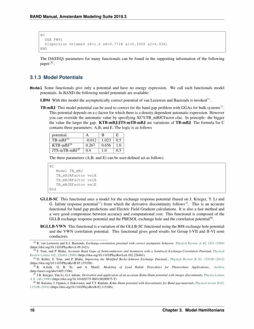
Model Some functionals give only a potential and have no energy expression. We call such functionals modelpotentials. In BAND the following model potentials are available:
LB94 With this model the asymptotically correct potential of van Leeuwen and Baerends is invoked32.
TB-mBJ This model potential can be used to correct for the band gap problem with GGAs for bulk systems33.This potential depends on a c-factor for which there is a density dependent automatic expression. Howeveryou can override the automatic value by specifying XC%TB_mBJCFactor cfac. In principle: the biggerthe value the larger the gap. KTB-mBJ/JTS-mTB-mBJ are variations of TB-mBJ. The formula for Ccontains three parameters: A,B, and E. The logic is as follows
potential A B ETB-mBJ33 -0.012 1.023 0.5KTB-mBJ34 0.267 0.656 1.0JTS-mTB-mBJ35 0.4 1.0 0.5
The three parameters (A,B, and E) can be user-defined set as follows:
XCModel TB_mBJTB_mBJAFactor valATB_mBJBFactor valBTB_mBJEFactor valE
End
GLLB-SC This functional uses a model for the exchange response potential (based on J. Krieger, Y. Li andG. Iafrate response potential37) from which the derivative discontinuity follows36. This is an accuratefunctional for band gap predictions and Electric Field Gradient calculations. It is also a fast method anda very good compromise between accuracy and computational cost. This functional is composed of theGLLB exchange response potential and the PBESOL exchange hole and the correlation potential36.
BGLLB-VWN This functional is a variation of the GLLB-SC functional using the B88 exchange hole potentialand the VWN correlation potential. This functional gives good results for Group I-VII and II-VI semiconductors.
32 R. van Leeuwen and E.J. Baerends, Exchange-correlation potential with correct asymptotic behavior. Physical Review A 49, 2421 (1994)(https://doi.org/10.1103/PhysRevA.49.2421).
33 F. Tran, and P. Blaha, Accurate Band Gaps of Semiconductors and Insulators with a Semilocal Exchange-Correlation Potential, PhysicalReview Letters 102, 226401 (2009) (https://doi.org/10.1103/PhysRevLett.102.226401).
34 D. Koller, F. Tran, and P. Blaha, Improving the Modified Becke-Johnson Exchange Potential., Physical Review B 83, 155109 (2012)(https://doi.org/10.1103/PhysRevB.85.155109).
35 R. A.Jishi, O. B. Ta, and A. Sharif, Modeling of Lead Halide Perovskites for Photovoltaic Applications., Archive(http://arxiv.org/abs/1405.1706).
37 J.B. Krieger, Yan Li, G.J. Iafrate, Derivation and application of an accurate Kohn-Sham potential with integer discontinuity, Physics LettersA 8, 146 (1990) (https://doi.org/10.1016/0375-9601(90)90975-T)
36 M. Kuisma, J. Ojanen, J. Enkovaara, and T.T. Rantala, Kohn-Sham potential with discontinuity for Band gap materials, Physical review B 82,115106 (2010) (https://doi.org/10.1103/PhysRevB.82.115106).
16 Chapter 3. Model Hamiltonians

BAND Manual, Amsterdam Modeling Suite 2019.3
BGLLB-LYP This functional is a variation of the GLLB-SC functional using the B88 exchange hole potentialand the LYP correlation potential. This functional gives good results for large band gap insulators.
One can change the K parameter for the GLLB functionals with the GLLBKParameter key:
XCModel [GLLB-SC|BGLLB-VWN|BGLLB-LYP]GLLBKParameter val
End
The default value is K=0.382 (value obtained from the electron gas model in the original publication).
3.1.4 Non-Collinear Approach
SpinOrbitMagnetization (Default=CollinearZ) Most XC functionals have as one ingredient the spin polar-ization. Normally the direction of the spin quantization axis is arbitrary and conveniently chosen to be the z-axis.However, in a spin-orbit (page 24) calculation the direction matters, and it is arbitrary to put the z-component ofthe magnetization vector into the XC functional. It is also possible to plug the size of the magnetization vectorinto the XC functional. This is called the non-collinear approach. There is also the exotic option to choosethe quantization axis along the x or y axis. To summarize, the value NonCollinear invokes the non-collinearmethod. The other three option CollinearX, CollinearY and CollinearZ causes either the x, y, or z componentto be used as spin polarization for the XC functional.
3.1.5 LibXC Library Integration
LibXC functional LibXC is a library of approximate XC functionals, see Ref.38. The development version 3of LibXC is used. See the LibXC website for the complete list of functionals: http://www.tddft.org/programs/Libxc.
The following functionals can be evaluated with LibXC (incomplete list):
• LDA: LDA, PW92, TETER93
• GGA: AM05, BGCP, B97-GGA1, B97-K, BLYP, BP86, EDF1, GAM, HCTH-93, HCTH-120, HCTH-147, HCTH-407, HCTH-407P, HCTH-P14, PBEINT, HTBS, KT2, MOHLYP, MOHLYP2, MPBE, MPW,N12, OLYP, PBE, PBEINT, PBESOL, PW91, Q2D, SOGGA, SOGGA11, TH-FL, TH-FC, TH-FCFO,TH-FCO, TH1, TH2, TH3, TH4, VV10, XLYP, XPBE, HLE16
• MetaGGA: B97M-V, M06-L, M11-L, MN12-L, MS0, MS1, MS2, MVS, PKZB, TPSS, HLE17
• Hybrids (only for non-periodic systems): B1LYP, B1PW91, B1WC, B3LYP, B3LYP*, B3LYP5,B3LYP5, B3P86, B3PW91, B97, B97-1 B97-2, B97-3, BHANDH, BHANDHLYP, EDF2, MB3LYP-RC04, MPW1K, MPW1PW, MPW3LYP, MPW3PW, MPWLYP1M, O3LYP, OPBE, PBE0, PBE0-13, REVB3LYP, REVPBE, RPBE, SB98-1A, SB98-1B, SB98-1C, SB98-2A, SB98-2B, SB98-2C,SOGGA11-X, SSB, SSB-D, X3LYP
• MetaHybrids (only for non-periodic systems): B86B95, B88B95, BB1K, M05, M05-2X, M06, M06-2X, M06-HF, M08-HX, M08-SO, MPW1B95, MPWB1K, MS2H, MVSH, PW6B95, PW86B95, PWB6K,REVTPSSH, TPSSH, X1B95, XB1K
• Range-separated (for periodic systems, only short range-separated functionals can be used, seeRange-separated hybrid functionals (page 18)): CAM-B3LYP, CAMY-B3LYP, HJS-PBE, HJS-PBESOL,HJS-B97X, HSE03, HSE06, LRC_WPBE, LRC_WPBEH, LC-VV10, LCY-BLYP, LCY-PBE, M11,MN12-SX, N12-SX, TUNED-CAM-B3LYP, WB97, WB97X, WB97X-V
38 M.A.L. Marques, M.J.T. Oliveira, and T. Burnus, Libxc: a library of exchange and correlation functionals for density functional theory,Computer Physics Communications 183, 2272 (2012) (https://doi.org/10.1016/j.cpc.2012.05.007).
3.1. Density Functional (XC) 17

BAND Manual, Amsterdam Modeling Suite 2019.3
Example usage for the MVS functional:
XCLibXC MVS
End
Notes:
• All electron basis sets should be used (see CORE NONE in section Basis set (page 41)).
• For periodic systems only short range-separated functionals can be used (see Range-separated hybridfunctionals (page 18))
• In case of LibXC the output of the BAND calculation will give the reference for the used functional, seealso the LibXC website http://www.tddft.org/programs/Libxc.
• Do not use any of the subkeys LDA, GGA, METAGGA, MODEL in combination with the subkey LIBXC.
• One can use the DISPERSION key icw LIBXC. For a selected number of functionals the optimized dis-persion parameters will be used automatically, please check the output in that case.
3.1.6 Range-separated hybrid functionals
Short range-separated hybrid functionals, like the HSE03 functional39, can be useful for prediction of more accurateband gaps compared to GGAs. These must be specified via the LibXC (page 17) key
XCLibXC functional omega=value
End
functional The functional to be used. (Incomplete) list of available functionals:HSE06, HSE03, HJS-B97X, HJS-PBE and HJS-PBESOL (See the LibXC website(http://www.tddft.org/programs/octopus/wiki/index.php/Libxc_functionals) for a complete list of availablefunctionals).
omega Optional. You can optionally specify the switching parameter omega of the range-separated hybrid. Onlypossible for the HSE03 and HSE06 functionals (See39).
Notes:
• Hybrid functionals can only be used in combination with all-electron basis sets (see CORE NONE in sectionBasis set (page 41)).
• The Hartree-Fock exchange matrix is calculated through a procedure known as Resolution of the Identity (RI).See RIHartreeFock (page 59) key.
• Regular hybrids (such as B3LYP) and long range-separated hybrids (such as CAM-B3LYP) cannot be used inperiodic boundary conditions calculations (they can only be used for non-periodic systems).
• There is some confusion in the scientific literature about the value of the switching parameter 𝜔 for the HSEfunctionals. In LibXC, and therefore in BAND, the HSE03 functional uses 𝜔 = 0.106066 while the HSE06functional uses 𝜔 = 0.11.
Usage example:
XCLibXC HSE06 omega=0.1
End
39 J. Heyd, G.E. Scuseria and M. Ernzerhof, Hybrid functionals based on a screened Coulomb potential, J. Chem. Phys. 118, 8207 (2003)(https://doi.org/10.1063/1.1564060).
18 Chapter 3. Model Hamiltonians

BAND Manual, Amsterdam Modeling Suite 2019.3
3.1.7 Defaults and special cases
• If the XC key is not used, the program will apply only the Local Density Approximation (no GGA terms). Thechosen LDA form is then VWN.
• If only a GGA part is specified, omitting the LDA subkey, the LDA part defaults to VWN, except when the LYPcorrelation correction is used: in that case the LDA default is Xonly: pure exchange.
• The reason for this is that the LYP formulas assume the pure-exchange LDA form, while for instance thePerdew-86 correlation correction is a correction to a correlated LDA form. The precise form of this correlatedLDA form assumed in the Perdew-86 correlation correction is not available as an option in ADF but the VWNformulas are fairly close to it.
• Be aware that typing only the subkey LDA, without an argument, will activate the VWN form (also if LYP isspecified in the GGA part).
3.1.8 GGA+U
A special way to treat correlation is with so-called LDA+U, or GGA+U calculations. It is intended to solve the bandgap problem of traditional DFT, the problem being an underestimation of band gaps for transition-metal complexes.A Hubbard like term is added to the normal Hamiltonian, to model on-site interactions. In its very simplest form itdepends on only one parameter, U, and this is the way it has been implemented in BAND. The energy expression isequation (11) in the work of Cococcioni41. See also the review article40.
HubbardUEnabled [True | False]LValue stringUValue stringPrintOccupations [True | False]
End
HubbardU
Type Block
Description Options for Hubbard-corrected DFT calculations.
Enabled
Type Bool
Default value False
Description Whether or not to apply the Hubbard Hamiltonian
LValue
Type String
Default value
Description For each atom type specify the l value (0 - s orbitals, 1 - p orbitals, 2 - d orbitals).A negative value is interpreted as no l-value.
UValue
Type String
41 M. Cococcioni, and S. de Gironcoli, Linear response approach to the calculation of the effective interaction parameters in the LDA+U method,Physical Review B 71, 035105 (2005) (https://doi.org/10.1103/PhysRevB.71.035105).
40 V.I. Anisimov, F. Aryasetiawan, and A.I. Lichtenstein, First-principles calculations of the electronic structure and spectra of strongly correlatedsystems: the LDA + U method, Journal Physics: Condensed Matter 9, 767 (1997) (https://doi.org/10.1088/0953-8984/9/4/002).
3.1. Density Functional (XC) 19

BAND Manual, Amsterdam Modeling Suite 2019.3
Default value
Description For each atom type specify the U value (in atomic units). A value of 0.0 is inter-preted as no U.
PrintOccupations
Type Bool
Default value True
Description Whether or not to print the occupations during the SCF.
An example to apply LDA+U to the d-orbitals of NiO looks like:
...Atoms
Ni 0.000 0.000 0.000O 2.085 2.085 2.085
End...
...HubbardU
printOccupations trueEnabled trueuvalue 0.3 0.0lvalue 2 -1
End...
3.1.9 OEP
(Expert options) When you are using a meta-GGA you are by default using a generalized Kohn-Sham method. How-ever, it is possible to calculate a local potential, as is required for a strict Kohn-Sham calculation, via OEP, (see42).
The main options are controlled with the MetaGGA subkey of the XC block if OEP is present.
XC[...]MetaGGA GGA OEP approximation Fit Potential[...]
End
GGA specifies the name of the used meta-GGA. In combination with OEP only PBE, TPSS, MVS, MS0, MS1, MS2,and SCAN can be used!
approximation (Default: KLI) There are three flavors to approximate the OEP: KLI, Slater, and ELP
Fit By adding the string Fit on this line, one uses the fitted density instead of the exact density for the evaluation.
Potential If not specified, only the tau-dependent part of the OEP is evaluated and used. By adding the stringPotential in addition the tau-independent part is added to the XC potential. (This is needed e.g. for plotting the‘vxc’)
With the following subkeys of the XC blockkey you have extra control over the iterative OEP evaluation:
MGGAOEPMaxIter (Default: 30) defines the maximum number of cycles for the iterative OEP evaluation.
42 Zeng-hui Yang, Haowei Peng, Jianwei Sun, and John P. Perdew, More realistic band gaps from meta-generalized gradient approximations:Only in a generalized Kohn-Sham scheme, Physical Review B 93, 205205 (2016) (https://doi.org/10.1103/PhysRevB.93.205205).
20 Chapter 3. Model Hamiltonians

BAND Manual, Amsterdam Modeling Suite 2019.3
MGGAOEPConvergence (Default: 1E-6) defines convergence criterion for OEP evaluation.
MGGAOEPWaitIter (Default: 0) defines the number of SCF cycles with the regular meta-GGA before switchingto the OEP scheme.
MGGAOEPMaxAbortIter (Default: 0) defines number of cycles for which the error is allowed to increase beforethe calculation is aborted. Here, zero means: do never abort.
MGGAOEPMaxErrorIncrease (Default: 0.0) defines the maximum rate of increasing error before the calculationis aborted. Here, zero means: do never abort.
An example for an OEP metaGGA calculation
XCMetaGGA MVS OEP
End
Note that a very fine Becke grid is needed.
BeckeGridQuality USERUserRadMulFactor 20.0UserCoreL 11UserInter1L 13UserInter2L 21UserExterL 31UserExterLBoost 35
End
Note also: the gaps are typically not closer to experiment, and the calculations are more expensive. This option ismainly about academic interest.
3.1.10 DFT-1/2
The DFT-1/2 method due to Slater has been extended by Ferreira (PRB,78,125116,2008(https://doi.org/10.1103/PhysRevB.78.125116)) to address the band gap problem. DFT-1/2 can be used incombination with any XC functional (this method is also referred to as LDA-1/2 or GGA-1/2, depending on thefunctional used).
The physical picture is that the hole is localized having substantial self energy. Adding an electron to the solid isassumed to go to a very delocalized state with little or no self energy. The method amounts to adding attractivespherical potentials at atomic sites and optimizing the screening parameter for maximal band gap, and can be used ontop of any functional, relativistic option and spin option. From this viewpoint the only freedom in the method is thelist of active atom types, the ones for which we will add the potential and optimize the gap. The l-dependent potentialoption from Ferreira is currently not supported.
The simplest approach is to optimize all the atom types. However, one can also look at the character of the top of thevalence band, and determine which atoms are contributing to the PDOS there. This can be done by hand by using thebandstructure GUI module. In band there is an option to analyze this automatically, see the Prepare=true sub option.
See also:
Example: DFT-1/2 method for Silicon (page 151)
XCDFTHalf
ActiveAtomTypeAtomType stringIonicCharge float
3.1. Density Functional (XC) 21

BAND Manual, Amsterdam Modeling Suite 2019.3
ScreeningCutOffs float_listEndEnabled [True | False]Prepare [True | False]SelfConsistent [True | False]
EndEnd
XC
DFTHalf
Type Block
Description DFT-1/2 method for band gaps. See PRB vol 78,125116 2008. This method can beused in combination with any functional. For each active atom type (see ActiveAtomType)Band will perform SCF calculations at different screening cut-off values (see ScreeningCut-Offs) and pick the cut-off value that maximizes the band gap. If multiple atom types areactive, the screening cut-off optimizations are done one type at the time (in the same orderas the ActiveAtomType blocks appear in the input).
ActiveAtomType
Type Block
Recurring True
Description Use the DFT-1/2 method for the atom-type specified in this block.
AtomType
Type String
Description Atom-type to use. You can activate all atom-types by specifying ‘All’.
IonicCharge
Type Float
Default value 0.5
Description The amount of charge to be removed from the atomic HOMO.
ScreeningCutOffs
Type Float List
Default value [0.0, 1.0, 2.0, 3.0, 4.0, 5.0]
Unit Bohr
Description List of screening cut-offs (to screen the asymptotic IonicCharge/r potential).Band will loop over these values and find the cut-off that maximizes the band-gap. If onlyone number is provided, Band will simply use that value.
Enabled
Type Bool
Default value False
GUI name Use method
Description Whether the DFT-1/2 method will be used.
Prepare
22 Chapter 3. Model Hamiltonians
BAND Manual, Amsterdam Modeling Suite 2019.3
Type Bool
Default value False
Description Analyze the band structure to determine reasonable settings for an DFT-1/2calculation. If this is possible the list of active atom types is written to the output. Thiscan be used in a next run as the values for ActiveAtomType. The DFTHalf%Enabled keyshould be set to false
SelfConsistent
Type Bool
Default value True
Description Apply the extra potential during the SCF, or only afterwards. Applying DFT-1/2only post SCF increases the band gap, compared to the self-consistent one.
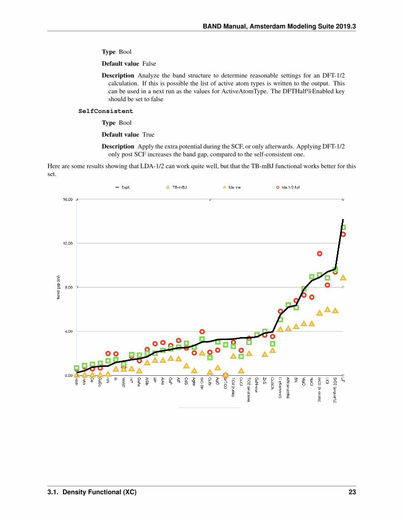
Here are some results showing that LDA-1/2 can work quite well, but that the TB-mBJ functional works better for thisset.
3.1. Density Functional (XC) 23

BAND Manual, Amsterdam Modeling Suite 2019.3
3.2 Relativistic Effects and Spin
3.2.1 Spin polarization
By default Band calculations are spin-restricted. You can instruct Band to perform a spin-unrestricted via theUnrestricted key:
Unrestricted [True | False]
Unrestricted
Type Bool
Default value False
Description Controls wheather Band should perform a spin-unrestricted calculation. Spin-unrestricted calculations are computationally roughly twice as expensive as spin-restricted.
The orbitals are occupied according to the aufbau principle.
If you want to enforce a specific spin-polarization (instead of occupying according to the aufbau principle) you canuse the EnforcedSpinPolarization key:
EnforcedSpinPolarization float
EnforcedSpinPolarization
Type Float
GUI name Spin polarization
Description Enforce a specific spin-polarization instead of occupying according to the aufbau prin-ciple. The spin-polarization is the difference between the number of alpha and beta electron.Thus, a value of 1 means that there is one more alpha electron than beta electrons. The numbermay be anything, including zero, which may be of interest when searching for a spin-flippedpair, that may otherwise end up in the (more stable) parallel solution.
3.2.2 Relativistic Effects
Relativistic effects are treated with the accurate and efficient ZORA approach12, controlled by the Relativistickeyword. Relativistic effects are negligible for light atoms, but grow to dramatic changes for heavy elements. A ruleof thumb is: Relativistic effects are quite small for elements of row 4, but very large for row 6 elements (and later).
RelativityLevel [None | Scalar | Spin-Orbit]
End
Relativity
Type Block
Description Options for relativistic effects.
Level1 P.H.T. Philipsen, E. van Lenthe, J.G. Snijders and E.J. Baerends, Relativistic calculations on the adsorption of CO on the (111) surfaces of Ni,
Pd, and Pt within the zeroth-order regular approximation. Physical Review B 56, 13556 (1997) (https://doi.org/10.1103/PhysRevB.56.13556).2 P.H.T. Philipsen, and E.J. Baerends, Relativistic calculations to assess the ability of the generalized gradient approximation to reproduce trends
in cohesive properties of solids. Physical Review B 61, 1773 (2000) (https://doi.org/10.1103/PhysRevB.61.1773).
24 Chapter 3. Model Hamiltonians

BAND Manual, Amsterdam Modeling Suite 2019.3
Type Multiple Choice
Default value None
Options [None, Scalar, Spin-Orbit]
GUI name Relativity (ZORA)
Description None: No relativistic effects. Scalar: Scalar relativistic ZORA. This option comesat very little cost. SpinOrbit: Spin-orbit coupled ZORA. This is the best level of theory, butit is (4-8 times) more expensive than a normal calculation. Spin-orbit effects are generallyquite small, unless there are very heavy atoms in your system, especially with p valenceelectrons (like Pb). See also the SpinOrbitMagnetization key.
See also the SpinOrbitMagnetization (page 17) key.
3.3 Solvation
Band offers two implicit solvent models, COSMO and SM12.
3.3.1 COSMO: Conductor like Screening Model and the Solvation-key
You can study chemistry in solution, as contrasted to the gas phase, with the implementation in BAND of the Conductorlike Screening Model (COSMO) of solvation1.
In the COSMO model all solvents are roughly the same, and approximated by an enveloping metal sheet. One explicitdependency on the solvent is that the solvation energy is scaled by
𝑓(𝜖) =𝜖− 1
𝜖 + 𝜒
and this depends on the dielectric constant of the solvent, and an empirical factor 𝜒. The other is that the shape of thesurface is influenced by the Rad parameter, see below.
The solvent information is specified in the solvent key of the solvation block. The simplest option is to use oneof the pre-defined solvents:
SolvationEnabled [True | False]Solvent
Name [...]End
End
Solvation
Type Block
Description Options for the COSMO (Conductor like Screening Model) solvation model.
Enabled
Type Bool
Default value False
GUI name Include COSMO solvation1 A. Klamt and G. Schüürmann, COSMO: a new approach to dielectric screening in solvents with explicit expressions for the screening energy
and its gradient. Journal of the Chemical Society: Perkin Transactions 2, 799 (1993) (https://doi.org/10.1039/P29930000799).
3.3. Solvation 25

BAND Manual, Amsterdam Modeling Suite 2019.3
Description Use the Conductor like Screening Model (COSMO) to include solvent effects.
Solvent
Type Block
Description Solvent details
Name
Type Multiple Choice
Default value Water
Options [AceticAcid, Acetone, Acetonitrile, Ammonia, Aniline, Benzene, BenzylAlco-hol, Bromoform, Butanol, isoButanol, tertButanol, CarbonDisulfide, CarbonTetrachlo-ride, Chloroform, Cyclohexane, Cyclohexanone, Dichlorobenzene, DiethylEther, Diox-ane, DMFA, DMSO, Ethanol, EthylAcetate, Dichloroethane, EthyleneGlycol, Formamide,FormicAcid, Glycerol, HexamethylPhosphoramide, Hexane, Hydrazine, Methanol,MethylEthylKetone, Dichloromethane, Methylformamide, Methypyrrolidinone, Nitroben-zene, Nitrogen, Nitromethane, PhosphorylChloride, IsoPropanol, Pyridine, Sulfolane,Tetrahydrofuran, Toluene, Triethylamine, TrifluoroaceticAcid, Water]
GUI name Solvent
Description Name of a pre-defined solvent. A solvent is characterized by the dielectricconstant (Eps) and the solvent radius (Rad).
This is the list of possible solvents and their corresponding Eps and Rad values:
Solvent Name Formula Eps RadAceticAcid CH3COOH 6.19 2.83Acetone CH3COCH3 20.7 3.08Acetonitrile CH3CN 37.5 2.76Ammonia NH3 16.9 2.24Aniline C6H5NH2 6.8 3.31Benzene C6H6 2.3 3.28BenzylAlcohol C6H5CH2OH 13.1 3.45Bromoform CHBr3 4.3 3.26Butanol C4H9OH 17.5 3.31isoButanol (CH3)2CHCH2OH 17.9 3.33tertButanol (CH3)3COH 12.4 3.35CarbonDisulfide CS2 2.6 2.88CarbonTetrachloride CCl4 2.2 3.37Chloroform CHCl3 4.8 3.17Cyclohexane C6H12 2 3.5Cyclohexanone C6H10O 15 3.46Dichlorobenzene C6H4Cl2 9.8 3.54DiethylEther (CH3CH2)2O 4.34 3.46Dioxane C4H8O2 2.2 3.24DMFA (CH3)2NCHO 37 3.13DMSO (CH3)2SO 46.7 3.04Ethanol CH3CH2OH 24.55 2.85EthylAcetate CH3COOCH2CH3 6.02 3.39Dichloroethane ClCH2CH2Cl 10.66 3.15EthyleneGlycol HOCH2CH2OH 37.7 2.81Formamide HCONH2 109.5 2.51
Continued on next page
26 Chapter 3. Model Hamiltonians

BAND Manual, Amsterdam Modeling Suite 2019.3
Table 3.1 – continued from previous pageFormicAcid HCOOH 58.5 2.47Glycerol C3H8O3 42.5 3.07HexamethylPhosphoramide C6H18N3OP 43.3 4.1Hexane C6H14 1.88 3.74Hydrazine N2H4 51.7 2.33Methanol CH3OH 32.6 2.53MethylEthylKetone CH3CH2COCH3 18.5 3.3Dichloromethane CH2Cl2 8.9 2.94Methylformamide HCONHCH3 182.4 2.86Methypyrrolidinone C5H9NO 33 3.36Nitrobenzene C6H5NO2 34.8 3.44Nitrogen N2 1.45 2.36Nitromethane CH3NO2 35.87 2.77PhosphorylChloride POCl3 13.9 3.33IsoPropanol (CH3)2CHOH 19.9 3.12Pyridine C5H5N 12.4 3.18Sulfolane C4H8SO2 43.3 3.35Tetrahydrofuran C4H8O 7.58 3.18Toluene C6H5CH3 2.38 3.48Triethylamine (CH3CH2)3N 2.44 3.81TrifluoroaceticAcid CF3COOH 8.55 3.12Water H2O 78.39 1.93
Several other options can be defined in the Solvation block:
SolvationCVec [EXACT | FITPOT]Charge
Conv floatCorr [True | False]Iter integerMethod [CONJ | INVER]
EndEnabled [True | False]Radii # Non-standard block. See details.
...EndSCF [VAR | PERT | NONE]Solvent
Del floatEmp floatEps floatName [...]Rad float
EndSurf [Delley | Wsurf | Asurf | Esurf | Klamt]
End
Solvation
Type Block
Description Options for the COSMO (Conductor like Screening Model) solvation model.
CVec
3.3. Solvation 27

BAND Manual, Amsterdam Modeling Suite 2019.3
Type Multiple Choice
Default value EXACT
Options [EXACT, FITPOT]
GUI name Calculate Coulomb interaction
Description Choose how to calculate the Coulomb interaction matrix between the molecule andthe point charges on the surface: - EXACT: use exact density, and integrate against thepotential of the point charges. This may have inaccuracies when integration points are closeto the point charges. - FITPOT: evaluate the molecular potential at the positions of the pointcharges, and multiply with these charges.
Charge
Type Block
Description Select the algorithm to determine the charges.
Conv
Type Float
Default value 1e-08
Description Charge convergence threshold in iterative COSMO solution.
Corr
Type Bool
Default value True
GUI name Correct for outlying charge
Description Correct for outlying charge.
Iter
Type Integer
Default value 1000
Description Maximum number of iterations to solve COSMO equations.
Method
Type Multiple Choice
Default value CONJ
Options [CONJ, INVER]
GUI name Charge determination method
Description INVER: matrix inversion, CONJ: biconjugate gradient method. The CONJmethod is guaranteed to converge with small memory requirements and is normally thepreferred method.
Enabled
Type Bool
Default value False
GUI name Include COSMO solvation
Description Use the Conductor like Screening Model (COSMO) to include solvent effects.
28 Chapter 3. Model Hamiltonians

BAND Manual, Amsterdam Modeling Suite 2019.3
Radii
Type Non-standard block
Description The values are the radii of the atomic spheres. If not specified the default values arethose by Allinge. Format: ‘AtomType value’. e.g.: ‘H 0.7’
SCF
Type Multiple Choice
Default value VAR
Options [VAR, PERT, NONE]
GUI name Handle charges
Description Determine the point charges either Variational (VAR) or after the SCF as a Pertur-bation (PERT).
Solvent
Type Block
Description Solvent details
Del
Type Float
Description Del is the value of Klamt’s delta_sol parameter, only relevant in case of Klamtsurface.
Emp
Type Float
Description Emp is the empirical scaling factor x for the energy scaling.
Eps
Type Float
Description User-defined dielectric constant of the solvent (overrides the Eps value of thesolvent defined in ‘Name’)
Name
Type Multiple Choice
Default value Water
Options [AceticAcid, Acetone, Acetonitrile, Ammonia, Aniline, Benzene, BenzylAlco-hol, Bromoform, Butanol, isoButanol, tertButanol, CarbonDisulfide, CarbonTetrachlo-ride, Chloroform, Cyclohexane, Cyclohexanone, Dichlorobenzene, DiethylEther, Diox-ane, DMFA, DMSO, Ethanol, EthylAcetate, Dichloroethane, EthyleneGlycol, Formamide,FormicAcid, Glycerol, HexamethylPhosphoramide, Hexane, Hydrazine, Methanol,MethylEthylKetone, Dichloromethane, Methylformamide, Methypyrrolidinone, Nitroben-zene, Nitrogen, Nitromethane, PhosphorylChloride, IsoPropanol, Pyridine, Sulfolane,Tetrahydrofuran, Toluene, Triethylamine, TrifluoroaceticAcid, Water]
GUI name Solvent
Description Name of a pre-defined solvent. A solvent is characterized by the dielectricconstant (Eps) and the solvent radius (Rad).
Rad
3.3. Solvation 29
BAND Manual, Amsterdam Modeling Suite 2019.3
Type Float
Unit Angstrom
Description User-defined radius of the solvent molecule (overrides the Rad value of thesolvent defined in ‘Name’).
Surf
Type Multiple Choice
Default value Delley
Options [Delley, Wsurf, Asurf, Esurf, Klamt]
GUI name Surface type
Description Within the COSMO model the molecule is contained in a molecule shaped cavity.Select one of the following surfaces to define the cavity: - Wsurf: Van der Waals surface -Asurf: solvent accessible surface - Esurf: solvent excluding surface - Klamt: Klamt surface- Delley: Delley surface.
3.3.2 Additional keys for periodic systems
For the simulation of periodic structures ICW solvation, you may specify the following options:
PeriodicSolvationRemovePointsWithNegativeZ [True | False]NStar integer
End
PeriodicSolvation
Type Block
Description Additional options for simulations of periodic structures with solvation.
RemovePointsWithNegativeZ
Type Bool
Default value False
GUI name Only above slab
Description Whether the COSMO surface is constructed on both sides of a surface. If one isonly interested in the solvation effect on the upper side of a surface (in the Z direction), thenthis option should be set to ‘True’
NStar
Type Integer
Default value 4
Description This option, expecting an integer number (>2), handles the accuracy for the con-struction of the COMSO surface. The larger the given number the more accurate the con-struction.
General remarks: The accuracy of the result and the calculation time is influenced by the screening radiusSCREENING%RMADEL (see Screening (page 67) block). If the calculation does take too long, defining a smallerradius does help. But: too small radii, especially smaller than the lattice constants, will give unphysical results.
30 Chapter 3. Model Hamiltonians
BAND Manual, Amsterdam Modeling Suite 2019.3
3.3.3 SM12: Solvation Model 12
Continuum solvation can be done with the Minnesota’s Solvation Model 12 (SM12) (JCTC,9,609,2013(https://pubs.acs.org/doi/10.1021/ct300900e)). Details on the implementation of SM12 in ADF can be found in Ref.(JCTC,12,4033,2016 (https://pubs.acs.org/doi/10.1021/acs.jctc.6b00410)). The energetics of solvation is calculatedusing:
∆𝐺⊗𝑆 = ∆𝐸𝐸 + 𝐺𝑃 + 𝐺𝐶𝐷𝑆 + ∆𝐺𝑁 + ∆𝐺⊗
𝑐𝑜𝑛𝑐
where the symbol ⊗ denotes an arbitrary choice of standard states, ∆𝐸𝐸 is the change in the solute’s internal electronicenergy in transferring from the gas phase to the liquid phase at the same geometry, 𝐺𝑃 is the polarization free energyof the solute–solvent system when the solute is inserted, 𝐺𝐶𝐷𝑆 is the component of the free energy that is nominallyassociated with cavitation, dispersion, and solvent structure, ∆𝐺𝑁 is the change in ∆𝐺0
𝑆 due to a change in nuclearcoordinates, and ∆𝐺⊗
𝑐𝑜𝑛𝑐 accounts for the difference in concentrations, if any, in the gas-phase standard state and thesolution-phase one. In case of 1 M concentration in both solution and gas, then ∆𝐺⊗
𝑆 = 0 kcal/mol, which yields∆𝐺*
𝑆 . If the same geometry is used in solution and gas phase calculation, then ∆𝐺𝑁 is zero.
SM12 makes use of the Generalized Born approximation to calculate the bulk electrostatic contribution. This iscomprised of several terms that are together known as the ENP (Electronic, Nuclear, and Polarization) term 𝐺𝑃 . TheSM12 model in Band uses CM5. CM5 is a class 4 charge model, making use of both empirical and density relatedterms. It is comprised of Hirshfeld charges, a simple bond order calculation, atomic distances, and atom specificparameters. The covalent radii utilized are based on the atomic covalent radius from the Handbook of Chemistry andPhysics. The Coulomb integral is described with the use of an approximation from Still et al.. Several parametersgo into describing this, which include: inter atomic distance, an empirical Born constant, and the Born area, whichis calculated with the Analytical Surface Area (ASA) algorithm. The Born area is calculated using Legendre-Gaussquadrature from the atomic radii to a sphere that encapsulates the entire molecule.
The ASA algorithm is also used to calculate the solvent accessible surface area (SASA), which is computed within theCDS (Cavitation, Dispersion, Solvation) term of SM12. The CDS term depends on three terms:
• SASA (ASA Algorithm)
• Atomic surface tension
• Macroscopic surface tension
Atomic surface tension is based on atom-atom distances and the solvent. Macroscopic surface tension is solventspecific. The SM12 implementation in Band reports energies in an atom specific way. You can attribute exact CDSand polarization energies to each atom in your solute. The parameters for SM12 are derived to explicitly incorporateorganic elements (N, C, O, F, Si, P, S, Cl, Br, I), with less emphasis on non-organics. Also, while most solvents havea generic atomic surface tension reliance for atoms, water has it’s own explicit set of parameters to better describe it.
Input
The minimal input for the SM12 method is the following:
SolvationSM12Enabled [True | False]Solv [...]
End
SolvationSM12
Type Block
Description Options for Solvation Model 12 (SM12).
Enabled
3.3. Solvation 31

BAND Manual, Amsterdam Modeling Suite 2019.3
Type Bool
Default value False
GUI name Include SM12 solvation
Description Whether to use the Solvation Model 12 (SM12) in the calculation.
Solv
Type Multiple Choice
Default value WATER
Options [ACETICACID, ACETONITRILE, ACETOPHENONE, ANILINE, ANISOLE,BENZENE, BENZONITRILE, BENZYLALCOHOL, BROMOBENZENE,BROMOETHANE, BROMOFORM, BROMOOCTANE, N-BUTANOL, SEC-BUTANOL, BUTANONE, BUTYLACETATE, N-BUTYLBENZENE, SEC-BUTYLBENZENE, T-BUTYLBENZENE, CARBONDISULFIDE, CARBON-TETRACHLORIDE, CHLOROBENZENE, CHLOROFORM, CHLOROHEX-ANE, M-CRESOL, CYCLOHEXANE, CYCLOHEXANONE, DECALIN,DECANE, DECANOL, 1-2-DIBROMOETHANE, DIBUTYLETHER, O-DICHLOROBENZENE, 1-2-DICHLOROETHANE, DIETHYLETHER, DIISO-PROPYLETHER, N-N-DIMETHYLACETAMIDE, N-N-DIMETHYLFORMAMIDE,2-6-DIMETHYLPYRIDINE, DIMETHYLSULFOXIDE, DODECANE, ETHANOL,ETHOXYBENZENE, ETHYLACETATE, ETHYLBENZENE, FLUOROBENZENE,1-FLUORO-N-OCTANE, HEPTANE, HEPTANOL, HEXADECANE, HEXADE-CYLIODIDE, HEXANE, HEXANOL, IODOBENZENE, ISOBUTANOL, ISOOC-TANE, ISOPROPANOL, ISOPROPYLBENZENE, P-ISOPROPYLTOLUENE,MESITYLENE, METHANOL, METHOXYETHANOL, METHYLENECHLORIDE,N-METHYLFORMAMIDE, 2-METHYLPYRIDINE, 4-METHYL-2-PENTANONE,NITROBENZENE, NITROETHANE, NITROMETHANE, O-NITROTOLUENE,NONANE, NONANOL, OCTANE, OCTANOL, PENTADECANE, PENTANE,PENTANOL, PERFLUOROBENZENE, PHENYLETHER, PROPANOL, PYRI-DINE, TETRACHLOROETHENE, TETRAHYDROFURAN, TETRAHYDROTHIO-PHENEDIOXIDE, TETRALIN, TOLUENE, TRIBUTYLPHOSPHATE, TRIETHY-LAMINE, 1-2-4-TRIMETHYLBENZENE, UNDECANE, WATER, XYLENE, 1-2-DIBROMOETHANE_WATER, 1-2-DICHLOROETHANE_WATER, BENZENE_WATER,CARBONTETRACHLORIDE_WATER, CHLOROBENZENE_WATER, CHLO-ROFORM_WATER, CYCLOHEXANE_WATER, DIBUTYLETHER_WATER, DI-ETHYLETHER_WATER, ETHYLACETATE_WATER, HEPTANE_WATER, HEX-ANE_WATER, NITROBENZENE_WATER, OCTANOL_WATER]
GUI name Solvent
Description List of predefined solvents
This is the full list of input options for the SM12 method:
SolvationSM12ARO floatAcid floatBase floatBornC floatBornRadiusConfig
MaxCellDistance floatPointsPerBohr integerUseLegendreGrid [True | False]
EndChgal float
32 Chapter 3. Model Hamiltonians

BAND Manual, Amsterdam Modeling Suite 2019.3
Cust stringDebug stringEPS floatEnabled [True | False]HALO floatKappa floatPostSCF [True | False]PrintSM12 [True | False]RadSolv floatRef floatSolv [...]Tens floatTopologicalExtrapolation
FirstCell integerLastCell integerOrder integer
EndEnd
SolvationSM12
Type Block
Description Options for Solvation Model 12 (SM12).
ARO
Type Float
Default value 0.0
Description Square of the fraction of non-hydrogen atoms in the solvent that are aromatic carbonatoms (carbon aromaticity)
Acid
Type Float
Default value 0.82
Description Abraham hydrogen bond acidity parameter
Base
Type Float
Default value 0.35
Description Abraham hydrogen bond bacicity parameter
BornC
Type Float
Default value 3.7
Description Coulomb constant for General Born Approximation
BornRadiusConfig
Type Block
Description
MaxCellDistance
3.3. Solvation 33

BAND Manual, Amsterdam Modeling Suite 2019.3
Type Float
Default value 30.0
Unit Bohr
Description Max distance from the centra cell used when computing the Born radii for pe-riodic systems
PointsPerBohr
Type Integer
Default value 10
Description
UseLegendreGrid
Type Bool
Default value True
Description
Chgal
Type Float
Default value 2.474
Description Exponential of Pauli’s bond order
Cust
Type String
Description Custom solvent input
Debug
Type String
Description Prints a lot of information about every pass on CDS and ENP code, keywords: ENP,CDS
EPS
Type Float
Default value 78.36
Description The dielectric constant
Enabled
Type Bool
Default value False
GUI name Include SM12 solvation
Description Whether to use the Solvation Model 12 (SM12) in the calculation.
HALO
Type Float
Default value 0.0
34 Chapter 3. Model Hamiltonians
BAND Manual, Amsterdam Modeling Suite 2019.3
Description Square of the fraction of non-hydrogen atoms in the solvent molecule that are F, Cl,or Br (electronegative halogenicity)
Kappa
Type Float
Default value 0.0
Description Factor for Debye screening
PostSCF
Type Bool
Default value False
Description Whether to apply the solvation potential during the SCF or only calculate the sol-vation energy after the SCF.
PrintSM12
Type Bool
Default value False
Description Prints out an in-depth breakdown of solvation energies
RadSolv
Type Float
Default value 0.4
Description The radius distance between the solute and solvent
Ref
Type Float
Default value 1.3328
Description Refractive index of solvent
Solv
Type Multiple Choice
Default value WATER
Options [ACETICACID, ACETONITRILE, ACETOPHENONE, ANILINE, ANISOLE,BENZENE, BENZONITRILE, BENZYLALCOHOL, BROMOBENZENE,BROMOETHANE, BROMOFORM, BROMOOCTANE, N-BUTANOL, SEC-BUTANOL, BUTANONE, BUTYLACETATE, N-BUTYLBENZENE, SEC-BUTYLBENZENE, T-BUTYLBENZENE, CARBONDISULFIDE, CARBON-TETRACHLORIDE, CHLOROBENZENE, CHLOROFORM, CHLOROHEX-ANE, M-CRESOL, CYCLOHEXANE, CYCLOHEXANONE, DECALIN,DECANE, DECANOL, 1-2-DIBROMOETHANE, DIBUTYLETHER, O-DICHLOROBENZENE, 1-2-DICHLOROETHANE, DIETHYLETHER, DIISO-PROPYLETHER, N-N-DIMETHYLACETAMIDE, N-N-DIMETHYLFORMAMIDE,2-6-DIMETHYLPYRIDINE, DIMETHYLSULFOXIDE, DODECANE, ETHANOL,ETHOXYBENZENE, ETHYLACETATE, ETHYLBENZENE, FLUOROBENZENE,1-FLUORO-N-OCTANE, HEPTANE, HEPTANOL, HEXADECANE, HEXADE-CYLIODIDE, HEXANE, HEXANOL, IODOBENZENE, ISOBUTANOL, ISOOC-TANE, ISOPROPANOL, ISOPROPYLBENZENE, P-ISOPROPYLTOLUENE,MESITYLENE, METHANOL, METHOXYETHANOL, METHYLENECHLORIDE,
3.3. Solvation 35

BAND Manual, Amsterdam Modeling Suite 2019.3
N-METHYLFORMAMIDE, 2-METHYLPYRIDINE, 4-METHYL-2-PENTANONE,NITROBENZENE, NITROETHANE, NITROMETHANE, O-NITROTOLUENE,NONANE, NONANOL, OCTANE, OCTANOL, PENTADECANE, PENTANE,PENTANOL, PERFLUOROBENZENE, PHENYLETHER, PROPANOL, PYRI-DINE, TETRACHLOROETHENE, TETRAHYDROFURAN, TETRAHYDROTHIO-PHENEDIOXIDE, TETRALIN, TOLUENE, TRIBUTYLPHOSPHATE, TRIETHY-LAMINE, 1-2-4-TRIMETHYLBENZENE, UNDECANE, WATER, XYLENE, 1-2-DIBROMOETHANE_WATER, 1-2-DICHLOROETHANE_WATER, BENZENE_WATER,CARBONTETRACHLORIDE_WATER, CHLOROBENZENE_WATER, CHLO-ROFORM_WATER, CYCLOHEXANE_WATER, DIBUTYLETHER_WATER, DI-ETHYLETHER_WATER, ETHYLACETATE_WATER, HEPTANE_WATER, HEX-ANE_WATER, NITROBENZENE_WATER, OCTANOL_WATER]
GUI name Solvent
Description List of predefined solvents
Tens
Type Float
Default value 103.62
Description Macroscopic surface tension of the solvent at the air/solvent interface at 298K(cal*mol^-1*Ang^-2)
TopologicalExtrapolation
Type Block
Description Method to extrapolate the long range Coulomb potential, needed for periodic cal-culations
FirstCell
Type Integer
Default value 5
Description First cell for the topological extrapolation of the long range part of the CoulombPotential.
LastCell
Type Integer
Default value 10
Description Last cell for the topological extrapolation of the long range part of the CoulombPotential.
Order
Type Integer
Default value 3
Description Order of the topological extrapolation of the long range part of the CoulombPotential.
36 Chapter 3. Model Hamiltonians

BAND Manual, Amsterdam Modeling Suite 2019.3
3.4 Electric and Magnetic Fields
3.4.1 Electric Field
EFieldEz floatunit [Volt/Angstrom | a.u. | Volt/Bohr | Volt/meter]
End
EField
Type Block
Description Include a homogeneous, static, electric field in the z-direction (only possible for 0D,1D or 2D periodic systems)
Ez
Type Float
Default value 0.0
GUI name Electric field - Z
Description Strength of the electric field, in units as selected with the EField unit key.
unit
Type Multiple Choice
Default value Volt/Angstrom
Options [Volt/Angstrom, a.u., Volt/Bohr, Volt/meter]
Description Unit of the electric field Ez
The static field is explicitly handled in the determination of the orbital coefficients, energy, and gradients. If you applyit to any other property, such as the NMR shielding tensor, dielectric function, solvation energy, etc., the result isprobably not entirely correct (that is, it might not include the effect of the external filed). In case of doubt contact theSCM staff.
The effect of a magnetic filed can be approximated by the following potential: 𝜇𝐵𝑖, where 𝜇𝐵 is the Bohrmagneton, 𝑖 are the Pauli matrices and is the magnetic field. For Spin-unrestricted collinear (page 24) calculations,the spin is assumed to be aligned with the z-axis.
3.4.2 Magnetic Field
BFieldBx floatBy floatBz floatDipole [True | False]DipoleAtom integerMethod [NR_SDOTB | NR_LDOTB | NR_SDOTB_LDOTB]Unit [tesla | a.u.]
End
BField
Type Block
3.4. Electric and Magnetic Fields 37

BAND Manual, Amsterdam Modeling Suite 2019.3
Description The effect of a magnetic filed can be approximated by the following potential: mu* sigma_i * B, where mu is the Bohr magneton, sigma_i are the Pauli matrices and B is themagnetic field
Bx
Type Float
Default value 0.0
Unit Tesla
Description Value of the x component of the BField
By
Type Float
Default value 0.0
Unit Tesla
Description Value of the y component of the BField
Bz
Type Float
Default value 0.0
Unit Tesla
Description Value of the z component of the BField
Dipole
Type Bool
Default value False
GUI name Bfield is: Atomic dipole
Description Use an atomic dipole as magnetic field instead of a uniform magnetic field.
DipoleAtom
Type Integer
Default value 1
GUI name on atom number
Description Atom on which the magnetic dipole should be centered (if using the dipole option)
Method
Type Multiple Choice
Default value NR_SDOTB
Options [NR_SDOTB, NR_LDOTB, NR_SDOTB_LDOTB]
Description There are two terms coupling to an external magnetic field. One is the intrinsic spinof the electron, called S-dot-B, the other one is the orbital momentum call L-dot-B. The L.Bis implemented non-relativistically, using GIAOs in the case of a homogeneous magneticfield (not for the dipole case).
Unit
Type Multiple Choice
38 Chapter 3. Model Hamiltonians
BAND Manual, Amsterdam Modeling Suite 2019.3
Default value tesla
Options [tesla, a.u.]
Description Unit of magnetic filed. The a.u. is the SI version of a.u.
3.4.3 Atoim-wise fuzzy potential
FuzzyPotential # Non-standard block. See details....
End
FuzzyPotential
Type Non-standard block
Description Atomic (fuzzy cell) based, external, electric potential. See example.
Example:
FuzzyPotentialscale $scalea1 v1 ! atom with index a1 gets potential coefficient v1 (a.u.)a2 v2 ! atom a2 gets potential v2...
End
scale Overall scaling factor to be applied.
If an atom is not in the list it gets a coefficient of zero. The potential of an atom is its number (𝑣𝑖) as specifiedon input times its fuzzy cell
𝑉 (𝑟) =
atoms∑𝑖
𝑣𝑖𝒫𝑖,𝑈 (𝑟)
using the same partition function 𝒫 as for the BeckeGrid (page 52). A partition function (or fuzzy cell) of anatom is close to one in the neighborhood of this atom.
The sign convention is: negative is favorable for electrons. (Unit: a.u.)
3.5 Nuclear Model
NuclearModel [PointCharge | Gaussian | Uniform]
NuclearModel
Type Multiple Choice
Default value PointCharge
Options [PointCharge, Gaussian, Uniform]
Description Specify what model to use for the nucleus. For the Gaussian model the nuclear radius iscalculated according to the work of Visscher and Dyall (L. Visscher, and K.G. Dyall, Dirac-Fockatomic electronic structure calculations using different nuclear charge distributions, Atomic Dataand Nuclear Data Tables 67, 207 (1997))
3.5. Nuclear Model 39

BAND Manual, Amsterdam Modeling Suite 2019.3
40 Chapter 3. Model Hamiltonians
CHAPTER
FOUR
ACCURACY AND EFFICIENCY
Given a Model Hamiltonian (page 11), the most important aspects determining the accuracy of a Band calculation are:
• Basis set (page 41)
• K-Space (page 49)
Also important, but to a lesser degree, are the following aspects:
• Numerical Integration (BeckeGrid) (page 52)
• Density fitting (ZlmFit) (page 56)
• Basis-set confinement (SoftConfinement) (page 46)
• SCF convergence (Convergence) (page 62)
• Hartree–Fock Resolution of the Identity (RIHartreeFock) (page 59) (only for hybrid functionals)
The CPU time and memory requirements strongly depends on these options, as does the accuracy of the results.
General NumericalQuality
A simple way of tweaking the accuracy of the calculation is via the NumericalQuality key. This sets the quality ofseveral technical aspects of a Band calculation (with the notable exception of the basis set (page 41))
NumericalQuality [Basic | Normal | Good | VeryGood | Excellent]
NumericalQuality
Type Multiple Choice
Default value Normal
Options [Basic, Normal, Good, VeryGood, Excellent]
Description Set the quality of several important technical aspects of a BAND calculation (with thenotable exception of the basis set). It sets the quality of: BeckeGrid (numerical integration),ZlmFit (density fitting), KSpace (reciprocal space integration), and SoftConfinement (basis setconfinement). Note: the quality defined in the block of a specific technical aspects supersedesthe value defined in NumericalQuality (e.g. if I specify ‘NumericalQuality Basic’ and ‘Beck-eGrid%Quality Good’, the quality of the BeckeGrid will be ‘Good’)
4.1 Basis set
Band represents the single-determinant electronic wave functions as a linear combinations of atom-centered basis func-tions (the basis set). See also: Wikipedia page on Basis Sets (https://en.wikipedia.org/wiki/Basis_set_(chemistry)).
41

BAND Manual, Amsterdam Modeling Suite 2019.3
The basis sets in Band consists of NAOs (Numerical Atomic Orbitals, obtained by solving numerically the Kohn-Shamequations for the isolated spherical atoms) augmented by a set of STOs (Slater Type Orbitals).
The choice of basis set is very important, as it influences heavily the accuracy, the CPU time and the memory usageof the calculation. Band comes with 6 predefined types of basis sets: SZ, DZ, DZP, TZP, TZ2P, QZ4P (SZ: SingleZeta, DZ: Double Zeta, DZP: Double Zeta + Polarization, TZP: Triple Zeta + Polarization, TZ2P: Triple Zeta +Double Polarization, QZ4P: Quadruple Zeta + Quadruple Polarization). See the sections Which basis set should I use?(page 42) and Available Basis Sets (page 45) for more details.
To speed up the calculation, Band can use the frozen core approximation in which core orbitals are kept frozenduring the SCF procedure (and the valence orbitals are orthogonalized against the frozen orbitals). One can run anall electron calculation by specifying Core None in the Basis input block. Note: some features, such as Hybridfunctionals (page 18), are incompatible with the frozen-core approximation, and require an all electron (i.e. CoreNone) basis set.
4.1.1 Basis input block
You can specify which basis set to use in the Basis input block.
BasisType [SZ | DZ | DZP | TZP | TZ2P | QZ4P]Core [None | Small | Medium | Large]
End
Basis
Type Block
Description Definition of the basis set
Type
Type Multiple Choice
Default value DZ
Options [SZ, DZ, DZP, TZP, TZ2P, QZ4P]
Description The basis sets to be used.
Core
Type Multiple Choice
Default value Large
Options [None, Small, Medium, Large]
Description Size of the frozen core.
4.1.2 Which basis set should I use?
The hierarchy of basis sets, from the smallest and least accurate (SZ) to the largest and most accurate (QZ4P), is SZ <DZ < DZP < TZP < TZ2P < QZ4P.
The choice of basis set is in general a trade off between accuracy and computation time: the more accurate the basisset, the more computationally demanding the calculation will be (both in term of CPU time and the memory usage).
42 Chapter 4. Accuracy and Efficiency

BAND Manual, Amsterdam Modeling Suite 2019.3
As an example, in the following table we compare accuracy v.s. CPU time for a (24,24) carbon nanotube usingdifferent basis sets. “Energy error” is defined as the absolute error in the formation energy per atom using the QZ4Presults as reference.1
Table 4.1: Accuracy and CPU time ratio for a (24,24) carbon nanotubeusing different basis sets
Basis Set Energy Error [eV] CPU time ratio (relative to SZ)SZ 1.8 1DZ 0.46 1.5DZP 0.16 2.5TZP 0.048 3.8TZ2P 0.016 6.1QZ4P reference 14.3
It is worthwhile noting that the error in formation energies are to some extend systematic, and they partially canceleach other out when taking energy differences. For example, if one considers the difference in energy between twocarbon nanotubes variants ((24,24) and (24-0)) with the same number of atoms, the basis set error is smaller than 1milli-eV/atom already with a DZP basis set, which is much smaller than the absolute error in the individual energies.The same consideration holds for reactions barriers: the error in the energy difference between different conformationsis much smaller than the error in the absolute energies themselves.
Band gaps:
The following figure shows the convergence WRT basis set of band gaps (XC:PBE). While DZ is often inaccurate(since DZ lacks any polarization function, the description of the virtual orbital space is very poor), TZP captures thetrends very well.
In general, since the basis set might have different effects on different properties, it is advisable to run a few simplecalculations to get an idea of the effect of the basis set with your property of interest.
A summary of the basis sets:
• SZ: Single Zeta, the minimal basis set (only NAOs), serves mostly a technical purpose. The results are ratherinaccurate, but it’s computationally efficient. It can be useful for running a very quick test calculation. See alsoSingle-Zeta-SCF-Restart link xxx.
• DZ: The Double Zeta basis set is computationally very efficient. It can be used for pre-optimization of structures(that should then be further optimized with a better basis set). Since it has no polarization functions, propertiesdepending on the virtual orbital space will be rather inaccurate.
• DZP: Double zeta plus polarization function. Only available for main group elements up to Krypton. Forother elements a TZP basis set will be used automatically. This is a reasonably good basis set for geometryoptimizations of organic systems.
• TZP: The Triple Zeta plus Polarization basis set offers the best balance between performance and accuracy.This is the basis set we would generally recommend.
• TZ2P: The Triple Zeta plus Double Polarization basis set is an accurate basis set. It is qualitatively similar toTZP but quantitatively better. It should be used when a good description of the virtual orbital space is needed.
• QZ4P: Quadruple zeta plus Quadruple Polarization. This is the biggest basis set available. It can be used forbenchmarking.
Frozen core:1 Computational details: Single Point calculation, ‘Good’ NumericalQuality, no frozen core, 7 k-points, XC functional: GGA:PBE. Calculation
performed on a 24 cores compute node. 96 atoms in the unit cell.
4.1. Basis set 43

BAND Manual, Amsterdam Modeling Suite 2019.3
Fig. 4.1: Convergence of Band Gaps WRT basis set for various system. (XC:PBE, K-Space Quality: Good)
44 Chapter 4. Accuracy and Efficiency

BAND Manual, Amsterdam Modeling Suite 2019.3
In general, the frozen core approximation does not influence the results significantly (especially if one uses a smallfrozen core). For accurate results on certain properties (like Properties at Nuclei (page 83)) all electron basis sets areneeded on the atoms of interest.
• For Meta-GGA XC functionals, it is recommended to use small or none frozen core (the frozen orbitals arecomputed using LDA and not the selected Meta-GGA)
• For optimizations under pressure, use small or none frozen core
4.1.3 Available Basis Sets
The basis set files, containing the definition of the basis set, are located in $ADFHOME/atomicdata/band.
The next table gives an indication frozen core (fc) standard basis sets are available for the different elements in BAND.Note that all electron (ae) basis set are available for all basis sets types.
Table 4.2: Available standard basis sets for non-relativistic and ZORA calculationsH-Uuo (Z=1-118)
Element frozen core SZ, DZ DZP TZP, TZ2P, QZ4PH-He (Z=1-2) ae Yes Yes YesLi-Ne (Z=3-10) ae .1s Yes Yes YesNa-Mg (Z=11-12) ae .1s .2p Yes Yes YesAl-Ar (Z=13-18) ae .2p Yes Yes YesK-Ca (Z=19-20) ae .2p .3p Yes Yes YesSc-Zn (Z=21-30) ae .2p .3p Yes YesGa-Kr (Z=31-36) ae .3p .3d Yes Yes YesRb-Sr (Z=37-38) ae .3p .3d .4p Yes YesY-Cd (Z=39-48) ae .3d .4p Yes YesIn-Ba (Z=49-56) ae .4p .4d Yes YesLa-Lu (Z=57-71) ae .4d .5p Yes YesHf-Hg (Z=72-80) ae .4d .4f Yes YesTl (Z=81) ae .4d .4f .5p Yes YesPb-Rn (Z=82-86) ae .4d .4f .5p .5d Yes YesFr-Ra (Z=87-88) ae .5p .5d Yes YesAc-Lr (Z=89-103) ae .5d .6p Yes YesRf-Uuo(Z=104-118) ae .5d .5f Yes Yes
• element name (without suffix): all electron (ae)
• .1s frozen: 1s
• .2p frozen: 1s 2s 2p
• .3p frozen: 1s 2s 2p 3s 3p
• .3d frozen: 1s 2s 2p 3s 3p 3d
• .4p frozen: 1s 2s 2p 3s 3p 3d 4s 4p
• .4d frozen: 1s 2s 2p 3s 3p 3d 4s 4p 4d
• .4f frozen: 1s 2s 2p 3s 3p 3d 4s 4p 4d 4f
• .5p frozen: 1s 2s 2p 3s 3p 3d 4s 4p 4d 5s 5p (La-Lu)
• .5p frozen: 1s 2s 2p 3s 3p 3d 4s 4p 4d 4f 5s 5p (other)
• .5d frozen: 1s 2s 2p 3s 3p 3d 4s 4p 4d 4f 5s 5p 5d
4.1. Basis set 45
BAND Manual, Amsterdam Modeling Suite 2019.3
• .6p frozen: 1s 2s 2p 3s 3p 3d 4s 4p 4d 4f 5s 5p 5d 6s 6p (Ac-Lr)
• .5f frozen: 1s 2s 2p 3s 3p 3d 4s 4p 4d 4f 5s 5p 5d 5f 6s 6p
Note: Not all combinations of basis set Type and Core are available for all elements. If a specific combination isnot available, Band will pick the first better basis set.
4.1.4 More Basis input options
BasisFolder stringByAtomType # Non-standard block. See details.
...End
End
Basis
Type Block
Description Definition of the basis set
Folder
Type String
Description Path to a folder containing the basis set files. This can be used for special use-defined basis sets. Cannot be used in combination with ‘Type’
ByAtomType
Type Non-standard block
Description Definition of the basis set for specific atom types (one definition per line). Format:‘AtomType Type=Type Core=Core’. Example: ‘C.large_basis Type=TZ2P Core=None’
See also: Example: Multiresolution (page 154).
4.1.5 Confinement of basis functions
It is possible to alter the radial part of the basis functions in order to make them more compact, which will in turnspeeds up the calculation.
SoftConfinementQuality [Auto | Basic | Normal | Good | VeryGood | Excellent]Radius floatDelta float
End
SoftConfinement
Type Block
Description In order to make the basis functions more compact, the radial part of the basis functionsis multiplied by a Fermi-Dirac (FD) function (this ‘confinement’ is done for efficiency and nu-merical stability reasons). A FD function goes from one to zero, controlled by two parameters.It has a value 0.5 at Radius, and the decay width is Delta.
46 Chapter 4. Accuracy and Efficiency

BAND Manual, Amsterdam Modeling Suite 2019.3
Quality
Type Multiple Choice
Default value Auto
Options [Auto, Basic, Normal, Good, VeryGood, Excellent]
GUI name Confinement
Description In order to make the basis functions more compact, the radial part of the basis func-tions is multiplied by a Fermi-Dirac (FD) function (this ‘confinement’ is done for efficiencyand numerical stability reasons). A FD function goes from one to zero, controlled by twoparameters. It has a value 0.5 at Radius, and the decay width is Delta. This key sets thetwo parameters ‘Radius’ and ‘Delta’. Basic: Radius=7.0, Delta=0.7; Normal: Radius=10.0,Delta=1.0; Good: Radius=20.0, Delta=2.0; VeryGood and Excellent: no confinement at all.If ‘Auto’, the quality defined in the ‘NumericalQuality’ will be used.
Radius
Type Float
Unit Bohr
Description Explicitely specify the radius parameter of the Fermi-Dirac function.
Delta
Type Float
Unit Bohr
Description Explicitely specify the delta parameter of the Fermi-Dirac function (if not specified,it will be 0.1*Radius).
• For geometry optimizations under pressure, Basic soft confinement is recommended.
4.1.6 Manually specifying AtomTypes (expert option)
AtomType (block-type) (Expert Option) Description of the atom type. Contains the block keys Dirac,BasisFunctions and FitFunctions. The key corresponds to one atom type. The ordering of theAtomType keys (in case of more than one atom type) is NOT arbitrary. It is interpreted as correspondingto the ordering of the Atoms keys. The n-th AtomType key supplies information for the numerical atom ofthe nth type, which in turn has atoms at positions defined by the nth Atoms key.
AtomType ElementSymbolDirac ChemSym
option...shells coresshell_specification occupation_number...
EndBasisFunctions
shell_specification STO_exponent...
EndFitFunctions
shell_specification STO_exponent...
4.1. Basis set 47
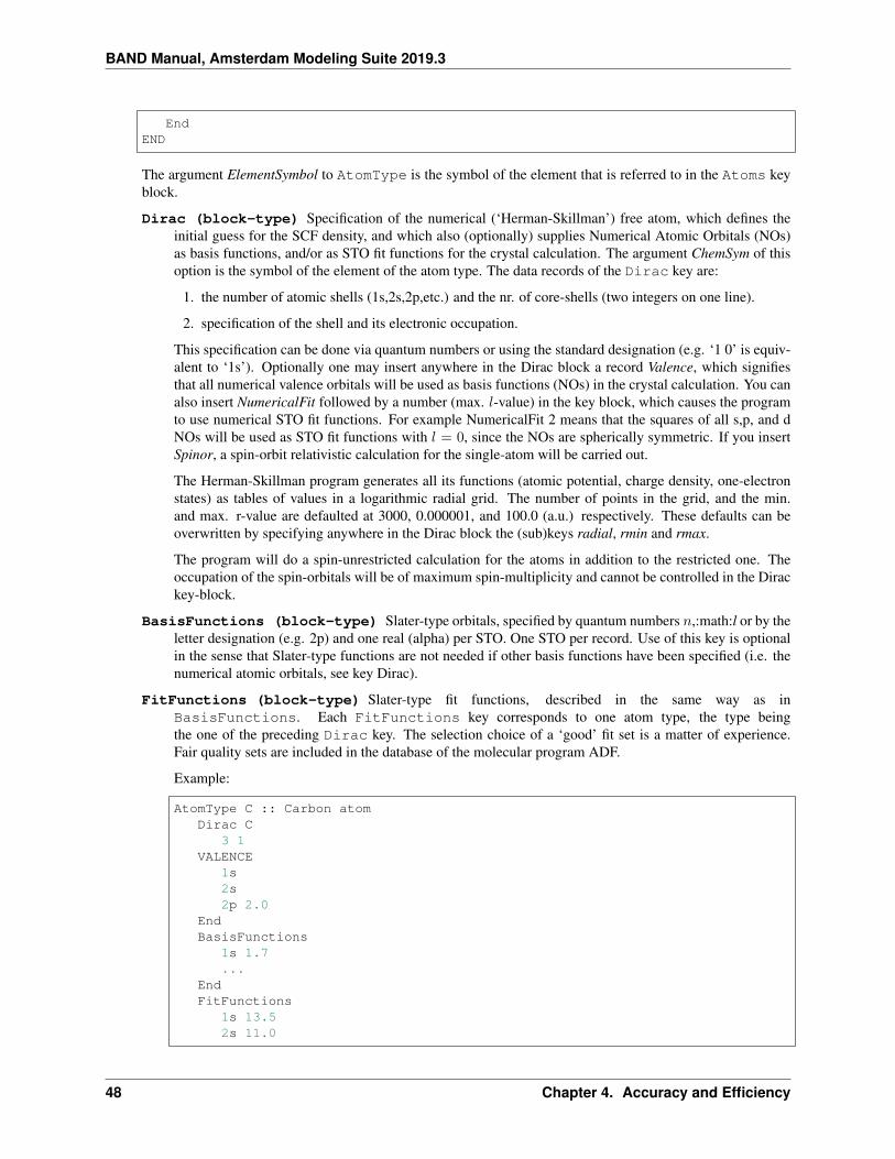
BAND Manual, Amsterdam Modeling Suite 2019.3
EndEND
The argument ElementSymbol to AtomType is the symbol of the element that is referred to in the Atoms keyblock.
Dirac (block-type) Specification of the numerical (‘Herman-Skillman’) free atom, which defines theinitial guess for the SCF density, and which also (optionally) supplies Numerical Atomic Orbitals (NOs)as basis functions, and/or as STO fit functions for the crystal calculation. The argument ChemSym of thisoption is the symbol of the element of the atom type. The data records of the Dirac key are:
1. the number of atomic shells (1s,2s,2p,etc.) and the nr. of core-shells (two integers on one line).
2. specification of the shell and its electronic occupation.
This specification can be done via quantum numbers or using the standard designation (e.g. ‘1 0’ is equiv-alent to ‘1s’). Optionally one may insert anywhere in the Dirac block a record Valence, which signifiesthat all numerical valence orbitals will be used as basis functions (NOs) in the crystal calculation. You canalso insert NumericalFit followed by a number (max. 𝑙-value) in the key block, which causes the programto use numerical STO fit functions. For example NumericalFit 2 means that the squares of all s,p, and dNOs will be used as STO fit functions with 𝑙 = 0, since the NOs are spherically symmetric. If you insertSpinor, a spin-orbit relativistic calculation for the single-atom will be carried out.
The Herman-Skillman program generates all its functions (atomic potential, charge density, one-electronstates) as tables of values in a logarithmic radial grid. The number of points in the grid, and the min.and max. r-value are defaulted at 3000, 0.000001, and 100.0 (a.u.) respectively. These defaults can beoverwritten by specifying anywhere in the Dirac block the (sub)keys radial, rmin and rmax.
The program will do a spin-unrestricted calculation for the atoms in addition to the restricted one. Theoccupation of the spin-orbitals will be of maximum spin-multiplicity and cannot be controlled in the Dirackey-block.
BasisFunctions (block-type) Slater-type orbitals, specified by quantum numbers 𝑛,:math:l or by theletter designation (e.g. 2p) and one real (alpha) per STO. One STO per record. Use of this key is optionalin the sense that Slater-type functions are not needed if other basis functions have been specified (i.e. thenumerical atomic orbitals, see key Dirac).
FitFunctions (block-type) Slater-type fit functions, described in the same way as inBasisFunctions. Each FitFunctions key corresponds to one atom type, the type beingthe one of the preceding Dirac key. The selection choice of a ‘good’ fit set is a matter of experience.Fair quality sets are included in the database of the molecular program ADF.
Example:
AtomType C :: Carbon atomDirac C
3 1VALENCE
1s2s2p 2.0
EndBasisFunctions
1s 1.7...
EndFitFunctions
1s 13.52s 11.0
48 Chapter 4. Accuracy and Efficiency

BAND Manual, Amsterdam Modeling Suite 2019.3
...End
End
TestFunctions (block-type) An optional subkey of the AtomType key block is TestFunctionswhich has the same format as the BasisFunctions and FitFunctions blocks. TheTestFunctions block specifies STOs to be used as test functions in the numerical integration package.For the time being the 𝑙 value is ignored. A possible application is to include a very tight function, toincrease the accuracy near a nucleus.
4.1.7 Basis Set Superposition Error (BSSE)
The Ghost Atom feature enables the calculation of Basis Set Superposition Errors (BSSE). Normally, if you want toknow the bonding energy of system A with system B you calculate three energies
1. 𝐸(𝐴 + 𝐵)
2. 𝐸(𝐴)
3. 𝐸(𝐵)
The bond energy is then 𝐸(𝐴 + 𝐵) − 𝐸(𝐴) − 𝐸(𝐵)
The BSSE correction is about the idea that we can also calculate E(A) including basis functions from molecule B.
You can make a ghost atom by simply adding “Gh.” in front of the element name, for instance “Gh.H” for a ghosthydrogen , “Gh.C” for a ghost Carbon atom.
You will get a better bonding energy, closer to the basis set limit by calculating
𝐸(𝐴 + 𝐵) − 𝐸(A with B as ghost) − 𝐸(B with A as ghost)
The BSSE correction is
𝐸(𝐴) − 𝐸(A with B as ghost) + 𝐸(𝐵) − 𝐸(B with A as ghost)
See also:
Example: BSSE correction (page 156)
4.2 K-Space
The K-Space sampling (i.e., the k-points used to sample the Brillouin Zone) is an important technical aspect of Band,as it influences heavily the accuracy, the CPU time and the memory usage of the calculation (see section Recommen-dations for k-space (page 52)).
4.2.1 KSpace input block
The K-Space can be controlled via the KSpace input block. Two different k-space integration methods are available:the Regular Grid (default) and the Symmetric Grid.
KSpaceType [Regular | Symmetric]Quality [Auto | GammaOnly | Basic | Normal | Good | VeryGood | Excellent]
End
KSpace
4.2. K-Space 49

BAND Manual, Amsterdam Modeling Suite 2019.3
Type Block
Description Options for the k-space integration (i.e. the grid used to sample the Brillouin zone)
Type
Type Multiple Choice
Default value Regular
Options [Regular, Symmetric]
GUI name K-space grid type
Description The type of k-space integration grid used to sample the Brillouin zone (BZ) used.‘Regular’: simple regular grid. ‘Symmetric’: symmetric grid for the irreducible wedge ofthe first BZ (useful when high-symmetry points in the BZ are needed to capture the correctphysics of the system, graphene being a notable example).
Quality
Type Multiple Choice
Default value Auto
Options [Auto, GammaOnly, Basic, Normal, Good, VeryGood, Excellent]
GUI name K-space
Description Select the quality of the K-space grid used to sample the Brillouin Zone. If ‘Auto’,the quality defined in the ‘NumericalQuality’ will be used. If ‘GammaOnly’, only one point(the gamma point) will be used. The actual number of K points generated depends on thisoption and on the size of the unit cell. The larger the real space cell, the fewer K points willbe generated. The CPU-time and accuracy strongly depend on this option.
Regular K-Space grid
By default, Band will look at the size of a lattice vectors and the KSpace quality to determine the number of k-points.The larger the lattice vector in real space, the smaller the reciprocal space vectors are, and as a result fewer k-pointsare needed. The following intervals will be distinguished: 0-5 Bohr, 5-10 Bohr, 10-20 Bohr, 20-50 Bohr, and beyond.Here is the table explaining how many k-points will be used along a lattice vector.
Lattice vector length Basic Normal Good VeryGood Excellent0-5 Bohr 5 9 13 17 215-10 Bohr 3 5 9 13 1710-20 Bohr 1 3 5 9 1320-50 Bohr 1 1 3 5 950- Bohr... 1 1 1 3 5
By preferring odd-numbered values we can use a quadratic interpolation method, and have the Γ point in the grid. Itis then reasonable to assume a decaying error when going to a better quality setting.
It is also possible to manually specify the number of k-space points along each reciprocal lattice vector
KSpaceRegular
NumberOfPoints integer_listEnd
End
KSpace
50 Chapter 4. Accuracy and Efficiency

BAND Manual, Amsterdam Modeling Suite 2019.3
Type Block
Description Options for the k-space integration (i.e. the grid used to sample the Brillouin zone)
Regular
Type Block
Description Options for the regular k-space integration grid.
NumberOfPoints
Type Integer List
Description Use a regular grid with the specified number of k-points along each recipro-cal lattice vector. For 1D periodic systems you should specify only one number, for 2Dsystems two numbers, and for 3D systems three numbers.
Symmetric K-Space grid (tetrahedron method)
The tetrahedron method can be useful when high symmetry points in the BZ are needed to capture the correct physicsof the system, graphene being a notable example.
The number of k-points in the symmetric grid depends on the KSpace quality and on the length of the shortest latticevector.
It is also possible to manually specify the symmetric k-space integration parameter:
KSpaceSymmetric
KInteg integerEnd
End
KSpace
Type Block
Description Options for the k-space integration (i.e. the grid used to sample the Brillouin zone)
Symmetric
Type Block
Description Options for the symmetric k-space integration grid.
KInteg
Type Integer
GUI name Accuracy
Description Specify the accuracy for the Symmetric method. 1: absolutely minimal (onlythe G-point is used) 2: linear tetrahedron method, coarsest spacing 3: quadratic tetrahedronmethod, coarsest spacing 4,6,... (even): linear tetrahedron method 5,7.... (odd): quadraticmethod The tetrahedron method is usually by far inferior.
General Remark: The tetrahedron method samples the irreducible wedge of the first BZ, whereas the regular gridsamples the whole, first BZ. As a rule of thumb you need to choose roughly twice the value for the regular grid. Forexample kspace 2 compares to grid 4 4 4, kspace 3 to grid 5 5 5, etc.. Sticking to this rule the number of uniquek-points will be roughly similar.
4.2. K-Space 51

BAND Manual, Amsterdam Modeling Suite 2019.3
4.2.2 Recommendations for k-space
Which K-Space quality to use depends very much a) the system you are studying and b) the property you are interestedin. We strongly recommend you to test the effect of different K-Space qualities on your system and properties ofinterest.
As an example, in the following table we list the errors on formation energy and band gap for diamond using regulark-space grids of different qualities (using Excellent kSpace quality as reference).
Table 4.3: Accuracy of formation energy for diamond (primitive unitcell) using different KSpace grids
KSpace quality Energy error / atom [eV] CPU time ratioGamma-Only 3.3 1Basic 0.6 2Normal 0.03 6Good 0.002 16VeryGood 0.0001 35Excellent reference 64
It is worthwhile noting that the errors due to finite k-space sampling in formation energies are to some extend system-atic, and they partially cancel each other out when taking energy differences.
In general, metals (or narrow-gap semiconductor) require higher K-Space sampling than insulators. For insulatorsand wide-gap semiconductors, Normal K-Space quality often suffices. For Narrow-gap semiconductor and metals,Good K-Space quality is highly recommended. For geometry optimizations under pressure, Good K-Space quality isrecommended.
Furthermore for certain properties, such as band gaps, Normal K-Space quality might not be enough to obtain reliableresults. For example, in following figure we see how Normal K-Space quality is often not enough for computing bandgaps (especially for the narrow-gap semiconductor of the top panel). For band gap prediction, it is recommended touse Good K-Space quality.
4.3 Numerical Integration
Many of the integrals needed by Band are computed via numerical integration. See also: Wikipedia page on NumericalIntegration (https://en.wikipedia.org/wiki/Numerical_integration).
4.3.1 Becke Grid
The numerical integration grid is a refined version of the fuzzy cells integration scheme developed by Becke1. Theimplementation in BAND is described in Ref.2.
The quality of the Becke integration grid can be changed within the BeckeGrid block:
BeckeGridQuality [Auto | Basic | Normal | Good | VeryGood | Excellent]RadialGridBoost floatAtomDepQuality # Non-standard block. See details.
...
1 A.D. Becke, A multicenter numerical integration scheme for polyatomic molecules, Journal of Chemical Physics 88, 2547 (1988)(https://doi.org/10.1063/1.454033).
2 M. Franchini, P.H.T. Philipsen, L. Visscher, The Becke Fuzzy Cells Integration Scheme in the Amsterdam Density Functional Program Suite,Journal of Computational Chemistry 34, 1818 (2013) (https://doi.org/10.1002/jcc.23323).
52 Chapter 4. Accuracy and Efficiency

BAND Manual, Amsterdam Modeling Suite 2019.3
Fig. 4.2: Convergence of band gaps WRT the k-space quality set for various system. (XC:PBE, Basis:TZP)
4.3. Numerical Integration 53

BAND Manual, Amsterdam Modeling Suite 2019.3
EndEnd
BeckeGrid
Type Block
Description Options for the numerical integration grid, which is a refined version of the fuzzy cellsintegration scheme developed by Becke.
Quality
Type Multiple Choice
Default value Auto
Options [Auto, Basic, Normal, Good, VeryGood, Excellent]
Description Quality of the integration grid. For a description of the various qualities and theassociated numerical accuracy see reference. If ‘Auto’, the quality defined in the ‘Numeri-calQuality’ will be used.
RadialGridBoost
Type Float
Default value 1.0
Description The number of radial grid points will be boosted by this factor. Some XC func-tionals require very accurate radial integration grids, so BAND will automatically boost theradial grid by a factor 3 for the following numerically sensitive functionals: LibXC M05,LibXC M05-2X, LibXC M06-2X, LibXC M06-HF, LibXC M06-L, LibXC M08-HX, LibXCM08-SO, LibXC M11-L, LibXC MS0, LibXC MS1, LibXC MS2, LibXC MS2H, LibXCMVS, LibXC MVSH, LibXC N12, LibXC N12-SX, LibXC SOGGA11, LibXC SOGGA11-X, LibXC TH1, LibXC TH2, LibXC WB97, LibXC WB97X, MetaGGA M06L, MetaHybridM06-2X, MetaHybrid M06-HF, MetaGGA MVS.
AtomDepQuality
Type Non-standard block
Description One can define a different grid quality for each atom (one definition per line). Lineformat: ‘AtomIndex Quality’, e.g. ‘3 Good’ means that a grid of Good quality will be usedfor the third atom in input order. If the index of an atom is not present in the AtomDepQualitysection, the quality defined in the Quality key will be used
Example: Multiresolution (page 154) illustrates how to use the AtomDepQuality option.
Notes:
• The space-partition function used in BAND differs from the one described in Ref.2. The unnormalized partitionfunction used in the program is defined as (Ω𝐼 is an element-dependent parameter: 0.1 Bohr for H, 0.3 Bohr forHe-Xe and 0.6 Bohr for Cs-Uuo):
𝒫𝑖,𝑈 =
⎧⎪⎨⎪⎩1 if 𝑟𝑖,𝑈 < Ω𝐼
0 if ∃𝑗 : 𝑟𝑗,𝑈 < Ω𝐽
𝜂𝑖𝑒−2(𝑟𝑖,𝑈−Ω𝐼 )/𝑎0
(𝑟𝑖,𝑈−Ω𝐼)2elsewhere
• The Becke grid is not very well suited to calculate Voronoi deformation density (VDD) charges. For accuratecalculation of VDD charges the Voronoi integration scheme is recommended.
54 Chapter 4. Accuracy and Efficiency

BAND Manual, Amsterdam Modeling Suite 2019.3
4.3.2 Radial grid of NAOs
RadialDefaultsNR integerRMax floatRMin float
End
RadialDefaults
Type Block
Description Options for the logarithmic radial grid of the basis functions used in the subprogramDirac
NR
Type Integer
Default value 3000
Description Number of radial points. With very high values (like 30000) the Dirac subprogrammay not converge.
RMax
Type Float
Default value 100.0
Unit Bohr
Description Upper bound of the logarithmic radial grid
RMin
Type Float
Default value 1e-06
Unit Bohr
Description Lower bound of the logarithmic radial grid
4.3.3 Voronoi grid (deprecated)
It is possible to use an alternative numerical integration scheme to the Becke Grid, namely the Voronoi Grid.
IntegrationMethod [Becke | Voronoi]
IntegrationMethod
Type Multiple Choice
Default value Becke
Options [Becke, Voronoi]
Description Choose the real-space numerical integration method. Note: the Voronoi integrationscheme is deprecated.
The options for the Voronoi Grid are specified in the Integration block:
4.3. Numerical Integration 55
BAND Manual, Amsterdam Modeling Suite 2019.3
IntegrationAccInt float
End
Integration
Type Block
Description Options for the Voronoi numerical integration scheme. Deprecated. Use BeckeGridinstead.
AccInt
Type Float
Default value 3.5
Description General parameter controlling the accuracy of the Voronoi integration grid. A valueof 3 would be basic quality and a value of 7 would be good quality.
4.4 Density Fitting
The Coulomb potential in Band is computed using a method called density fitting. The density fitting scheme in BANDis called Zlm Fit, and it is described in reference1. The ZlmFit is also used to compute (when needed) the gradientand hessian of the electron density.
4.4.1 Zlm Fit
The idea behind Zlm Fit can be summarized as follows: the total electron density is split into localized atomic densities(in a similar way as the volume is partitioned in the Becke grid). These atomic densities are then approximated by acombination of radial spline functions and real spherical harmonics (Zlm), for which the Coulomb potential can beeasily computed.
ZlmFitQuality [Auto | Basic | Normal | Good | VeryGood | Excellent]AtomDepQuality # Non-standard block. See details.
...End
End
ZlmFit
Type Block
Description Options for the density fitting scheme ‘ZlmFit’.
Quality
Type Multiple Choice
Default value Auto
Options [Auto, Basic, Normal, Good, VeryGood, Excellent]
GUI name Spline Zlm fit
1 M. Franchini, P.H.T. Philipsen, E. van Lenthe, L. Visscher, Accurate Coulomb Potentials for Periodic and Molecular Systems through DensityFitting, Journal of Chemical Theory and Computation 10, 1994 (2014) (https://doi.org/10.1021/ct500172n).
56 Chapter 4. Accuracy and Efficiency

BAND Manual, Amsterdam Modeling Suite 2019.3
Description Quality of the density-fitting approximation. For a description of the various quali-ties and the associated numerical accuracy see reference. If ‘Auto’, the quality defined in the‘NumericalQuality’ will be used.
AtomDepQuality
Type Non-standard block
Description One can specify different ZlmFit-quality for different atoms, The syntax for thisfree block is ‘iAtom quality’, where iAtom is the index of the atom in input order. Forthe atoms that are not present in the AtomDepQuality sub-block, the quality defined in theQuality key will be used.
Example: Multiresolution (page 154) illustrates how to use the AtomDepQuality option.
Expert options
ZlmFitLMargin integerAllowBoost [True | False]DensityThreshold floatPartitionFunThreshold floatFGaussianW floatFGridSpacing floatFKSpaceCutOff floatFirstTopoCell integerLastTopoCell integerOrderTopoTrick integerNumStarsPartitionFun integer
End
ZlmFit
Type Block
Description Options for the density fitting scheme ‘ZlmFit’.
LMargin
Type Integer
Default value 4
Description User-defined l-margin, i.e., l_max for fitting is max(lMargin +l_max_basis_function, 2*l_max_basis_function)
AllowBoost
Type Bool
Default value True
Description Allow automatic atom-dependent tuning of maximum l of spherical harmonics ex-pansion. Whether or not this boost is needed for a given atom is based on an heuristicestimate of how complex the density around that atom is.
DensityThreshold
Type Float
Default value 1e-07
Description Threshold below which the electron density is considered to be negligible.
4.4. Density Fitting 57

BAND Manual, Amsterdam Modeling Suite 2019.3
PartitionFunThreshold
Type Float
Default value 0.0
Description Threshold for the partition functions: if an integration point has a partition functionweight smaller than this threshold, it will be discarded.
FGaussianW
Type Float
Default value 1.0
Description Only for 3D periodic systems. Width of the Gaussian functions replacing the S andP Zlms for Fourier transform.
FGridSpacing
Type Float
Description Only for 3D periodic systems. Spacing for the Fourier grid. By default, this dependson the quality.
FKSpaceCutOff
Type Float
Description Only for 3D periodic systems. Cut-off of the grid in k-space for the Fourier trans-form.
FirstTopoCell
Type Integer
Default value 5
Description First cell for the topological extrapolation of the long range part of the CoulombPotential.
LastTopoCell
Type Integer
Default value 10
Description Last cell for the topological extrapolation of the long range part of the CoulombPotential.
OrderTopoTrick
Type Integer
Default value 3
Description Order of the topological extrapolation of the long range part of the Coulomb Poten-tial.
NumStarsPartitionFun
Type Integer
Default value 5
Description Number of cell stars to consider when computing the partition function.
58 Chapter 4. Accuracy and Efficiency

BAND Manual, Amsterdam Modeling Suite 2019.3
4.4.2 STO Fit (Deprecated)
In previous version of BAND (pre2014) this was the default option, which is now replaced by Zlm Fit. It is still usedin the context of NMR and OldResponse calculations.
4.5 Hartree–Fock RI
The Hartree-Fock exchange matrix is calculated through a procedure known as Resolution of the Identity (RI). Theimplementation of the RI scheme in BAND is loosely based on work by Ren et al.1. For more information on hybridfunctionals in BAND, see the XC section (page 11).
Technical aspects of the RI scheme can be tweaked in the RIHartreeFock block:
RIHartreeFockQuality [VeryBasic | Basic | Normal | Good | VeryGood | Excellent]FitSetQuality [VeryBasic | Basic | Normal | Good | VeryGood | Excellent]DependencyThreshold floatAtomDepQuality # Non-standard block. See details.
...End
End
RIHartreeFock
Type Block
Description The Hartree-Fock exchange matrix is calculated through a procedure known as Reso-lution of the Identity (RI). Here you can tweak various parameters of the procedure.
Quality
Type Multiple Choice
Default value Normal
Options [VeryBasic, Basic, Normal, Good, VeryGood, Excellent]
GUI name RI Hartree-Fock
Description Accuracy of numerical integration and thresholds of the RI procedure.
FitSetQuality
Type Multiple Choice
Default value Normal
Options [VeryBasic, Basic, Normal, Good, VeryGood, Excellent]
Description The auxiliary fit set employed in the RI scheme. This is an important aspect ofthe procedure, significantly affecting both accuracy and computation time. For SZ and DZbasis set a ‘basic’ FitSetQuality will suffice. For ‘DZP’ and ‘TZP’ a normal quality is rec-ommended. For larger basis set, use either ‘normal’ or better FitSetQuality.
DependencyThreshold
Type Float
1 X. Ren, P. Rinke, V. Blum, J. Wieferink, A. Tkatchenko, A. Sanfilippo, K. Reuter and M. Scheffler, Resolution-of-identity approach toHartree–Fock, hybrid density functionals, RPA, MP2 and GW with numeric atom-centered orbital basis functions, New J. Phys. 14 053020(https://doi.org/10.1088/1367-2630/14/5/053020).
4.5. Hartree–Fock RI 59

BAND Manual, Amsterdam Modeling Suite 2019.3
Default value 0.001
Description To improve numerical stability, almost linearly-dependent combination of basisfunctions are removed from the Hartree-Fock exchange matrix. If the SCF does not con-verge or you obtain unphysically large bond energy in an Hybrid calculation, you might trysetting the DependencyThreshold to a larger value (e.g. 3.0E-3).
AtomDepQuality
Type Non-standard block
Description One can define a different fit-set quality for each atom. The syntax for this freeblock is ‘iAtom quality’, where iAtom is the index of the atom in input order.
For efficiency and numerical stability reasons, it is advisable to include:
SoftConfinementQuality Basic
End
See the Confinement of basis functions (page 46) section for more info.
Notes: for periodic systems it is only possible to use short-range hybrid functionals (e.g. HSE06) and all-electronbasis sets.
Note:
• In AMS2019.3 the fit set for FitSetQuality Good has been improved.
4.6 Self Consistent Field (SCF)
The SCF procedure searches for a self-consistent density. The self-consistent error is the square root of the integralof the squared difference between the input and output density of the cycle operator. When the SCF error is below acertain criterion, controlled by subkey Criterion of block key Convergence, convergence is reached. In case ofbad convergence the SCF looks at the subkeys Mixing, and Degenerate, and the subkeys of block key DIIS.
See also:
Troubleshooting: SCF does not converge (page 129)
4.6.1 SCF block
SCFEigenstates [True | False]Iterations integerMethod [DIIS | MultiSecant]Mixing floatPMatrix [True | False]Rate floatVSplit float
End
SCF
Type Block
60 Chapter 4. Accuracy and Efficiency

BAND Manual, Amsterdam Modeling Suite 2019.3
Description Controls technical SCF parameters.
Eigenstates
Type Bool
Description The program knows two alternative ways to evaluate the charge density iterativelyin the SCF procedure: from the P-matrix, and directly from the squared occupied eigenstates.By default the program actually uses both at least one time and tries to take the most efficient.If present, Eigenstates turns off this comparison and lets the program stick to one method(from the eigenstates).
Iterations
Type Integer
Default value 300
GUI name Maximum number of cycles
Description The maximum number of SCF iterations to be performed.
Method
Type Multiple Choice
Default value DIIS
Options [DIIS, MultiSecant]
Description Choose the general scheme used to converge the density in the SCF. In case of scfproblems one can try the MultiSecant alternative at no extra cost per SCF cycle. For moredetails see the DIIS and MultiSecantConfig block.
Mixing
Type Float
Default value 0.075
Description Initial ‘damping’ parameter in the SCF procedure, for the iterative update of thepotential: new potential = old potential + mix (computed potential-old potential). Note: theprogram automatically adapts Mixing during the SCF iterations, in an attempt to find theoptimal mixing value.
PMatrix
Type Bool
Description If present, evaluate the charge density from the P-matrix. See also the key Eigen-states.
Rate
Type Float
Default value 0.99
Description Minimum rate of convergence for the SCF procedure. If progress is too slow theprogram will take measures (such as smearing out occupations around the Fermi level, seekey Degenerate of block Convergence) or, if everything seems to fail, it will stop
VSplit
Type Float
Default value 0.05
4.6. Self Consistent Field (SCF) 61
BAND Manual, Amsterdam Modeling Suite 2019.3
Description To disturb degeneracy of alpha and beta spin MOs the value of this key is added tothe beta spin potential at the startup.
4.6.2 Convergence
All options and parameters related to the convergence behavior of the SCF procedure are defined in theConvergence block key. Also the finite temperature distribution is part of this
ConvergenceCriterion floatDegenerate stringElectronicTemperature floatInitialDensity [rho | psi]LessDegenerate [True | False]NoDegenerate [True | False]SpinFlip integer_liststartwithmaxspin [True | False]
End
Convergence
Type Block
Description Options and parameters related to the convergence behavior of the SCF procedure.
Criterion
Type Float
Description Criterion for termination of the SCF procedure. The default depends on the Numer-icalQuality and on the number of atoms in the system.
Degenerate
Type String
Default value default
Description Smooths (slightly) occupation numbers around the Fermi level, so as to insure thatnearly-degenerate states get (nearly-) identical occupations. Be aware: In case of problematicSCF convergence the program will turn this key on automatically, unless the key ‘Nodegen-erate’ is set in input. The smoothing depends on the argument to this key, which can beconsidered a ‘degeneration width’. When the argument reads default, the program will usethe value 1e-4 a.u. for the energy width.
ElectronicTemperature
Type Float
Default value 0.0
Unit a.u.
Description Simulates a finite-temperature electronic distribution using the defined energy. Thismay be used to achieve convergence in an otherwise problematically converging system.The energy of a finite-T distribution is different from the T=0 value, but for small T a fairapproximation of the zero-T energy is obtained by extrapolation. The extrapolation energycorrection term is printed with the survey of the bonding energy in the output file. Check thatthis value is not too large. Build experience yourself how different settings may affect theoutcomes. Note: this key is meant to help you overcome convergence problems, not to do
62 Chapter 4. Accuracy and Efficiency

BAND Manual, Amsterdam Modeling Suite 2019.3
finite-temperature research! Only the electronic distribution is computed T-dependent, otheraspects are not accounted for!
InitialDensity
Type Multiple Choice
Default value rho
Options [rho, psi]
Description The SCF is started with a guess of the density. There are the following choicesRHO: the sum of atomic density. PSI: construct an initial eigensystem by occupying theatomic orbitals. The guessed eigensystem is orthonormalized, and from this the density iscalculated/
LessDegenerate
Type Bool
Default value False
Description If smoothing of occupations over nearly degenerate orbitals is applied (see Degen-erate key), then, if this key is set in the input file, the program will limit the smoothing energyrange to 1e-4 a.u. as soon as the SCF has converged ‘halfway’, i.e. when the SCF error hasdecreased to the square root of its convergence criterion.
NoDegenerate
Type Bool
Default value False
Description This key prevents any internal automatic setting of the key DEGENERATE.
SpinFlip
Type Integer List
GUI name Flip spin for atoms
Description List here the atoms for which you want the initial spin polarization to be flipped.This way you can distinguish between ferromagnetic and anti ferromagnetic states. Cur-rently, it is not allowed to give symmetry equivalent atoms a different spin orientation. Toachieve that you have to break the symmetry.
startwithmaxspin
Type Bool
Default value True
Description To break the initial perfect symmetry of up and down densities there are two strate-gies. One is to occupy the numerical orbitals in a maximum spin configuration. The alterna-tive is to add a constant to the potential. See also Vsplit key.
4.6.3 DIIS
The DIIS procedure to obtain the SCF solution depends on several parameters. Default values can be overruled withthis block.
4.6. Self Consistent Field (SCF) 63

BAND Manual, Amsterdam Modeling Suite 2019.3
DIISAdaptable [True | False]CHuge floatCLarge floatCondition floatDiMix floatNCycleDamp integerNVctrx integerVariant [DIIS | LISTi | LISTb | LISTd]
End
DIIS
Type Block
Description Parameters for the DIIS procedure to obtain the SCF solution
Adaptable
Type Bool
Default value True
Description Change automatically the value of dimix during the SCF.
CHuge
Type Float
Default value 20.0
GUI name No DIIS (but damping) when coefs >
Description When the largest coefficient in the DIIS expansion exceeds this value, damping isapplied
CLarge
Type Float
Default value 20.0
GUI name Reduce DIIS space when coefs >
Description When the largest DIIS coefficient exceeds this value, the oldest DIIS vector is re-moved and the procedure re-applied
Condition
Type Float
Default value 1000000.0
Description The condition number of the DIIS matrix, the largest eigenvalue divided by thesmallest, must not exceed this value. If this value is exceeded, this vector will be removed.
DiMix
Type Float
Default value 0.2
GUI name Bias DIIS towards latest vector with
Description Mixing parameter for the DIIS procedure
NCycleDamp
64 Chapter 4. Accuracy and Efficiency

BAND Manual, Amsterdam Modeling Suite 2019.3
Type Integer
Default value 1
GUI name Do not start DIIS before cycle
Description Number of initial iterations where damping is applied, before any DIIS is consid-ered
NVctrx
Type Integer
Default value 20
GUI name Size of DIIS space
Description Maximum number of DIIS expansion vectors
Variant
Type Multiple Choice
Default value DIIS
Options [DIIS, LISTi, LISTb, LISTd]
Description Which variant to use. In case of problematic SCF convergence, first try MultiSe-cant, and if that does not work the LISTi is the advised method. Note: LIST is computation-ally more expensive per SCF iteration than DIIS.
4.6.4 Multi secant
MultiSecantConfigCMax floatInitialSigmaN floatMaxSigmaN floatMaxVectors integerMinSigmaN float
End
MultiSecantConfig
Type Block
Description Parameters for the Multi-secant SCF convergence method.
CMax
Type Float
Default value 20.0
GUI name Max coeff
Description Maximum coefficient allowed in expansion
InitialSigmaN
Type Float
Default value 0.1
GUI name Initial
Description This is a lot like a mix factor: bigger means bolder
4.6. Self Consistent Field (SCF) 65

BAND Manual, Amsterdam Modeling Suite 2019.3
MaxSigmaN
Type Float
Default value 0.3
GUI name Max
Description Upper bound for the SigmaN parameter
MaxVectors
Type Integer
Default value 20
GUI name Number of cycles to use
Description Maximum number of previous cycles to be used
MinSigmaN
Type Float
Default value 0.01
GUI name Min
Description Lower bound for the SigmaN parameter
4.6.5 DIRIS
In the DIRIS block, which has the same options as the DIIS block, you can specify the DIIS options to be used in theDirac subprogram, for numerical single atom calculations, which constructs the radial tables for the NAOs.
4.7 More Technical Settings
There are of course many other settings influencing the precision and performance. Usually the user does not need tocare about them.
4.7.1 Linear Scaling
TailsBas float
End
Tails
Type Block
Description Ignore function tails.
Bas
Type Float
Default value 1e-06
GUI name Basis functions
Description Cut off the basis functions when smaller than the specified threshold.
66 Chapter 4. Accuracy and Efficiency

BAND Manual, Amsterdam Modeling Suite 2019.3
4.7.2 Dependency
DependencyBasis floatCore floatCoreValence floatFit float
End
Dependency
Type Block
Description Criteria for linear dependency of the basis and fit set
Basis
Type Float
Default value 1e-08
GUI name Dependency criterion
Description Criteria for linear dependency of the basis: smallest eigenvalue of the overlap ma-trix of normalized Bloch functions.
Core
Type Float
Default value 0.98
Description The program verifies that the frozen core approximation is reasonable, by checkingthe smallest value of the overlap matrix of the core (Bloch) orbitals against this criterion.
CoreValence
Type Float
Default value 1e-05
Description Criterion for dependency of the core functions on the valence basis. The maximumoverlap between any two normalized functions in the two respective function spaces shouldnot exceed 1.0-corevalence
Fit
Type Float
Default value 5e-06
Description Criterion for dependency of the total set of fit functions. The value monitored isthe smallest eigenvalue of the overlap matrix of normalized Bloch sums of symmetrized fitfunctions.
4.7.3 Screening
Band performs many lattice summations which are in practice truncated. The two prime examples are the constructionof the Bloch basis and the calculation of the solvation potential. The precision of the lattice summations is controlledby the Screening key
4.7. More Technical Settings 67

BAND Manual, Amsterdam Modeling Suite 2019.3
ScreeningCutOff floatDMadel floatNoDirectionalScreening [True | False]RCelx floatRMadel float
End
Screening
Type Block
Description For the periodic solvation potential and for the old (not default anymore) fitting method,BAND performs lattice summations which are in practice truncated. The precision of the latticesummations is controlled by the options in this block.
CutOff
Type Float
Description Criterion for negligibility of tails in the construction of Bloch sums. Default de-pends on Accuracy.
DMadel
Type Float
Description One of the parameters that define the screening of Coulomb-potentials in latticesums. Depends by default on Accuracy, rmadel, and rcelx. One should consult the literaturefor more information
NoDirectionalScreening
Type Bool
Description Real space lattice sums of slowly (or non-) convergent terms, such as the Coulombpotential, are computed by a screening technique. In previous releases, the screening wasapplied to all (long-range) Coulomb expressions. Screening is only applied in the periodicitydirections. This key restores the original situation: screening in all directions
RCelx
Type Float
Description Max. distance of lattice site from which tails of atomic functions will be taken intoaccount for the Bloch sums. Default depends on Accuracy.
RMadel
Type Float
Description One of the parameters that define screening of the Coulomb potentials in latticesummations. Depends by default on Accuracy, dmadel, rcelx. One should consult the litera-ture for more information.
4.7.4 Direct (on the fly) calculation of basis and fit
BAND usually calculates basis functions and theirs derivatives on the fly. However, for small bulk systems it can befaster to write the information to disk. Then one can set the DirectBas key to false. (Default = true)
68 Chapter 4. Accuracy and Efficiency

BAND Manual, Amsterdam Modeling Suite 2019.3
ProgrammerDirectBas bool
End
4.7.5 Fermi energy search
FermiDelta floatEps floatMaxTry integer
End
Fermi
Type Block
Description Technical parameter used in determining the Fermi energy, which is carried out at eachcycle of the SCF procedure.
Delta
Type Float
Default value 0.0001
Description Convergence criterion: upper and lower bounds for the Fermi energy and the cor-responding integrated charge volumes must be equal within delta.
Eps
Type Float
Default value 1e-10
Description After convergence of the Fermi energy search procedure, a final estimate is definedby interpolation and the corresponding integrated charge volume is tested. It should be exact,to machine precision. Tested is that it deviates not more than eps.
MaxTry
Type Integer
Default value 15
Description Maximum number of attempts to locate the Fermi energy. The procedure is itera-tive in nature, narrowing the energy band in which the Fermi energy must lie, between anupper and a lower bound. If the procedure has not converged sufficiently within MaxTryiterations, the program takes a reasonable value and constructs the charge density by interpo-lation between the functions corresponding to the last used upper and lower bounds for theFermi energy.
4.7.6 Block size
CPVector integer
CPVector
Type Integer
4.7. More Technical Settings 69

BAND Manual, Amsterdam Modeling Suite 2019.3
Default value 128
GUI name Vectorlength (blocksize)
Description The code is vectorized and this key can be used to set the vector length
KGrpX integer
KGrpX
Type Integer
Default value 5
GUI name Number of K-points at once
Description Absolute upper bound on the number of k-points processed together. This only affectsthe computational performance.
70 Chapter 4. Accuracy and Efficiency

CHAPTER
FIVE
SPECTROSCOPY AND PROPERTIES
5.1 Frequencies and Phonons
Frequencies and Phonons and can be computed via numerical differentiation by the AMS diver. See the Normal Modessection or the Phonon section of the AMS manual.
Several thermodynamic properties, such as Zero-point Energy, Internal Energy, Entropy, Free Energy and SpecificHeat are computed by default when calculating Phonons.
5.2 Elastic Tensor
The elastic tensor (and related elastic properties such as Bulk modulus, Shear modulus and Young modulus) can becomputed via numerical differentiation by AMS. See the Elastic Tensor section of the AMS manual.
When calculating the elastic tensors using Band one should disable Symmetry (page 123).
5.3 Optical Properties: Time-Dependent Current DFT
Time-Dependent Current Density Functional Theory (TD-CDFT) is a theoretical framework for computing opticalresponse properties, such as the frequency-dependent dielectric function.
In this section, the TD-CDFT implementation for extended systems (1D, 2D and 3D) in BAND is described. The inputkeys are described in NewResponse (page 73) or in OldResponse (page 77).
Some examples are available in the $ADFHOME/examples/band directory and are discussed in the Examplessection.
• Tutorial: Silicon (OldResponse)
• Tutorial: MoS2 Monolayer (NewResponse)
• Example: TD-CDFT for bulk diamond (OldResponse) (page 198)
5.3.1 Insulators, semiconductors and metals
The TD-CDFT module enables the calculation of real and imaginary parts of the material property tensor 𝜒𝑒(𝜔), calledthe electric susceptibility. The electric susceptibility is related to the macroscopic dielectric function, 𝜀𝑀 (𝜔).
71

BAND Manual, Amsterdam Modeling Suite 2019.3
For semi-conductors and insulator, for which the bands are either fully occupied or fully unoccupied, the dielectricfunction 𝜀𝑀 (𝜔) comprises only of the so called interband component:
𝜀𝑀 (𝜔) = 1 + 4𝜋𝜒𝑒(𝜔)
In general 𝜒𝑒(𝜔) and 𝜀𝑀 (𝜔) are tensors. They, however, simplify to scalars in isotropic systems.
For metals, for which partially-occupied bands exist, there is a so called intraband component arising due to transitionswithin a partially-occupied band:
𝜀𝑀 (𝜔) = 1 + 4𝜋𝜒𝑒(𝜔) − 4𝜋𝑖𝜎𝑒(𝜔)/𝜔
5.3.2 Frequency dependent kernel
It is known that the exact Vignale-Kohn (VK) kernel greatly improves the static polarizabilities of infinite polymers andnanotubes (see reference (https://doi.org/10.1063/1.2102899)), but gives bad results for the optical spectra of semicon-ductors and metals. For the low frequency part one needs a frequency dependent kernel, since Drude-like tails are com-pletely absent in the adiabatic local density approximation (ALDA). With a modified VK kernel, which neglects 𝜇𝑥𝑐
so that it reduces to the ALDA form in the static limit (see reference (https://doi.org/10.1103/PhysRevB.74.245117)),much better results can be obtained. BAND currently only supports the modified VK kernel in either the QV or CNTparametrization, and it should only be used for metals.
5.3.3 EELS
From the macroscopic dielectric function it is possible to calculate the electron energy loss function (EELS). In trans-mission EELS one studies the inelastic scattering of a beam of high energy electrons by a target. The scattering ratesobtained in these experiments are related to the dynamical structure factor 𝑆(𝑞, 𝜔) [A1]. In the special case withwavevector 𝑞 = 0, 𝑆(𝑞, 𝜔) is related to the longitudinal macroscopic dielectric function. This is the long-wave limitof EELS. For isotropic system the dielectric function is simply a scalar (1/3Tr(𝜀𝑀 (𝜔)) ). In this case the long-wavelimit of the electron energy loss function assumes the trivial form
lim𝑞→0
2𝜋𝑆(𝑞, 𝜔)
𝑞2𝑉=
𝜀2𝜀21 + 𝜀22
with 𝜀1 and 𝜀2 as real and imaginary part of the dielectric function.
References
The three related Ph.D. theses, due to F. Kootstra (on TD-DFT for insulators), P. Romaniello (on TD-CDFT for metals),and A. Berger (on the Vignale-Kohn functional in extended systems) contain much background information, and canbe downloaded from the SCM website (http://www.scm.com).
The most relevant publications on this topic due to the former “Groningen” group of P.L. de Boeij are1234.
[A1] S. E. Schnatterly, in Solid State Physics Vol.34, edited by H. Ehrenreich, F. Seitz, and D. Turnbull (AcademicPress, Inc., New York, 1979).
1 F. Kootstra, P.L. de Boeij and J.G. Snijders, Efficient real-space approach to time-dependent density functional theory for the dielectric responseof nonmetallic crystals. Journal of Chemical Physics 112, 6517 (2000). (https://doi.org/10.1063/1.481315)
2 P. Romaniello and P.L. de Boeij, Time-dependent current-density-functional theory for the metallic response of solids. Physical Review B 71,155108 (2005) (https://doi.org/10.1103/PhysRevB.71.155108).
3 J.A. Berger, P.L. de Boeij and R. van Leeuwen, Analysis of the viscoelastic coefficients in the Vignale-Kohn functional: The cases of one- andthree-dimensional polyacetylene., Physical Review B 71, 155104 (2005) (https://doi.org/10.1103/PhysRevB.71.155104).
4 P. Romaniello and P.L. de Boeij, Relativistic two-component formulation of time-dependent current-density functional theory: application tothe linear response of solids., Journal of Chemical Physics 127, 174111 (2007) (https://doi.org/10.1063/1.2780146).
72 Chapter 5. Spectroscopy and Properties

BAND Manual, Amsterdam Modeling Suite 2019.3
5.3.4 Input Options
In the 2017 release of BAND there are two implementations of the TD-CDFT formalism. The original implementation,relying on obsolete algorithms of BAND, is accessible via the OldResponse (page 77) key block. The new codesection, relying on more modern algorithms of BAND, is accessible via the NewResponse (page 73), NewResponseSCF(page 75) and NewResponseKSpace (page 76) key blocks. The differences between the two flavors are summarized inthe following table:
OldResponse NewResponse3D-systems yes yes2D-systems no yes1D-systems (yes) yesSemiconductors yes yesMetals yes (yes)ALDA yes yesVignale-Kohn yes noBerger2015 (3D) yes yesScalar ZORA yes yesSpin Orbit ZORA yes no
Besides these differences, one should not expect both flavors to give the exact same result, if the reciprocal space limitis not reached! This can be explained by different approaches to evaluate the integration weights of single-particletransitions in reciprocal space.
Attention: Response properties converge slowly with respect to k-space sampling (number of k-points). Alwayscheck the convergence of 𝜀𝑀 with respect to K-Space (page 49) options!!!
NewResponse
The dielectric function is computed when the key block NewResponse (page 73) is present in the input. Severalimportant settings can be defined in this key block.
Additional details can be specified via the NewResponseKSpace (page 76) and NewResponseSCF (page 75) blocks.
NewResponseNFreq integerFreqLow floatFreqHigh floatEShift floatActiveESpace floatDensityCutOff floatActiveXYZ string
End
NewResponse
Type Block
Description The TD-CDFT calculation to obtain the dielectric function is computed when this blockis present in the input. Several important settings can be defined here.
NFreq
Type Integer
Default value 5
5.3. Optical Properties: Time-Dependent Current DFT 73

BAND Manual, Amsterdam Modeling Suite 2019.3
Description Number of frequencies for which a linear response TD-CDFT calculation is per-formed.
FreqLow
Type Float
Default value 1.0
Unit eV
Description Lower limit of the frequency range for which response properties are calculated.(omega_low)
FreqHigh
Type Float
Default value 3.0
Unit eV
Description Upper limit of the frequency range for which response properties are calculated(omega_high).
EShift
Type Float
Default value 0.0
Unit eV
GUI name Shift
Description Energy shift of the virtual crystal orbitals.
ActiveESpace
Type Float
Default value 5.0
Unit eV
GUI name Active energy space
Description Modifies the energy threshold (DeltaE^max_thresh = omega_high + Ac-tiveESpace) for which single orbital transitions (DeltaEpsilon_ia = Epsilon_a^virtual- Epsilon_i^occupied) are taken into account.
DensityCutOff
Type Float
Default value 0.001
GUI name Volume cutoff
Description For 1D and 2D systems the unit cell volume is undefined. Here, the volume iscalculated as the volume bordered by the isosurface for the value DensityCutoff of the totaldensity.
ActiveXYZ
Type String
Default value t
74 Chapter 5. Spectroscopy and Properties
BAND Manual, Amsterdam Modeling Suite 2019.3
Description Expects a string consisting of three letters of either ‘T’ (for true) or ‘F’ (for false)where the first is for the X-, the second for the Y- and the third for the Z-component of theresponse properties. If true, then the response properties for this component will be evaluated.
NewResponseSCFBootstrap integerCOApproach [True | False]COApproachBoost [True | False]Criterion floatDIIS [True | False]LowFreqAlgo [True | False]Mixing floatNCycle integerXC integer
End
NewResponseSCF
Type Block
Description Details for the linear-response self-consistent optimization cycle. Only influencing theNewResponse code.
Bootstrap
Type Integer
Default value 0
Description defines if the Berger2015 kernel (Bootstrap 1) is used or not (Bootstrap 0). If youchose the Berger2015 kernel, you have to set NewResponseSCF%XC to ‘0’. Since it shall beused in combination with the bare Coulomb response only. Note: The evaluation of responseproperties using the Berger2015 is recommend for 3D systems only!
COApproach
Type Bool
Default value True
Description The program automatically decides to calculate the integrals and induced densi-ties via the Bloch expanded atomic orbitals (AO approach) or via the cyrstal orbitals (COapproach). The option COApproach overrules this decision.
COApproachBoost
Type Bool
Default value False
GUI name CO Approach Boost
Description Keeps the grid data of the Crystal Orbitals in memory. Requires significantly morememory for a speedup of the calculation. One might have to use multiple computing nodesto not run into memory problems.
Criterion
Type Float
Default value 0.001
Description For the SCF convergence the RMS of the induced density change is tested. If thisvalue is below the Criterion the SCF is finished. Furthermore, one can find the calculated
5.3. Optical Properties: Time-Dependent Current DFT 75
BAND Manual, Amsterdam Modeling Suite 2019.3
electric susceptibility for each SCF step in the output and can therefore decide if the defaultvalue is too loose or too strict.
DIIS
Type Bool
Default value True
Description In case the DIIS method is not working, one can switch to plain mixing by settingDIIS to false.
LowFreqAlgo
Type Bool
Default value True
GUI name Low Frequency Algorithm
Description Numerically more stable results for frequencies lower than 1.0 eV. Note: for agraphene monolayer the conical intersection results in a very small band gap (zero band gapsemi-conductor). This leads ta a failing low frequency algorithm. One can then chose to usethe algoritm as originally proposed by Kootstra by setting the input value to false. But, thiscan result in unreliable results for frequencies lower than 1.0 eV!
Mixing
Type Float
Default value 0.2
Description Mixing value for the SCF optimization.
NCycle
Type Integer
Default value 20
GUI name Cycles
Description Number of SCF cycles for each frequency to be evaluated.
XC
Type Integer
Default value 1
Description Influences if the bare induced Coulomb response (XC 0) is used for the effective,induced potential or the induced potential derived from the ALDA kernel as well (XC 1).
NewResponseKSpaceEta floatSubSimp integer
End
NewResponseKSpace
Type Block
Description Modify the details for the integration weights evaluation in reciprocal space for eachsingle-particle transition. Only influencing the NewResponse code.
Eta
76 Chapter 5. Spectroscopy and Properties
BAND Manual, Amsterdam Modeling Suite 2019.3
Type Float
Default value 1e-05
Description Defines the small, finite imaginary number i*eta which is necessary in the contextof integration weights for single-particle transitions in reciprocal space.
SubSimp
Type Integer
Default value 3
Description determines into how many sub-integrals each integration around a k point is split.This is only true for so-called quadratic integration grids. The larger the number the betterthe convergence behavior for the sampling in reciprocal space. Note: the computing time forthe weights is linear for 1D, quadratic for 2D and cubic for 3D!
OldResponse
OldResponseBerger2015 [True | False]CNT [True | False]CNVI floatCNVJ floatEbndtl floatEnabled [True | False]Endfr floatIsz integerIyxc integerNewVK [True | False]Nfreq integerQV [True | False]Shift floatStatic [True | False]Strtfr float
End
OldResponse
Type Block
Description Options for the old TD-CDFT implementation.
Berger2015
Type Bool
Default value False
Description Use the parameter-free polarization functional by A. Berger (Phys. Rev. Lett. 115,137402). This is possible for 3D insulators and metals. Note: The evaluation of responseproperties using the Berger2015 is recommend for 3D systems only!
CNT
Type Bool
Description Use the CNT parametrization for the longitudinal and transverse kernels of the XCkernel of the homogeneous electron gas. Use this in conjunction with the NewVK option.
CNVI
5.3. Optical Properties: Time-Dependent Current DFT 77

BAND Manual, Amsterdam Modeling Suite 2019.3
Type Float
Default value 0.001
Description The first convergence criterion for the change in the fit coefficients for the fit func-tions, when fitting the density.
CNVJ
Type Float
Default value 0.001
Description the second convergence criterion for the change in the fit coefficients for the fitfunctions, when fitting the density.
Ebndtl
Type Float
Default value 0.001
Unit Hartree
Description the energy band tolerance, for determination which routines to use for calculatingthe numerical integration weights, when the energy band posses no or to less dispersion.
Enabled
Type Bool
Default value False
Description If true, the response function will be calculated using the old TD-CDFT implemen-tation
Endfr
Type Float
Default value 3.0
Unit eV
Description The upper bound frequency of the frequency range over which the dielectric func-tion is calculated
Isz
Type Integer
Default value 0
Description Integer indicating whether or not scalar zeroth order relativistic effects are in-cluded in the TDCDFT calculation. 0 = relativistic effects are not included, 1 = rela-tivistic effects are included. The current implementation does NOT work with the optionXC%SpinOrbitMagnetization equal NonCollinear
Iyxc
Type Integer
Default value 0
Description integer for printing yxc-tensor (see http://aip.scitation.org/doi/10.1063/1.1385370).0 = not printed, 1 = printed.
NewVK
78 Chapter 5. Spectroscopy and Properties
BAND Manual, Amsterdam Modeling Suite 2019.3
Type Bool
Description Use the slightly modified version of the VK kernel (see https://aip.scitation.org/doi/10.1063/1.1385370). When using this option one uses effectively the static option, even formetals, so one should check carefully the convergence with the KSPACE parameter.
Nfreq
Type Integer
Default value 5
Description the number of frequencies for which a linear response TD-CDFT calculation isperformed.
QV
Type Bool
Description Use the QV parametrization for the longitudinal and transverse kernels of the XCkernel of the homogeneous electron gas. Use this in conjunction with the NewVK option.(see reference).
Shift
Type Float
Default value 0.0
Unit eV
Description energy shift for the virtual crystal orbitals.
Static
Type Bool
Description An alternative method that allows an analytic evaluation of the static response (nor-mally the static response is approximated by a finite small frequency value). This optionshould only be used for non-relativistic calculations on insulators, and it has no effect onmetals. Note: experience shows that KSPACE convergence can be slower.
Strtfr
Type Float
Default value 1.0
Unit eV
Description is the lower bound frequency of the frequency range over which the dielectric func-tion is calculated.
5.4 ESR/EPR
BAND is capable to calculate electron paramagnetic resonance (EPR) parameters for paramagnetic defects in solids:hyperfine A-tensor and the Zeeman g-tensor.
5.4. ESR/EPR 79
BAND Manual, Amsterdam Modeling Suite 2019.3
The implementation of EPR parameters in BAND is described in the publications by Kadantsev and co-workers1 and2.
Hyperfine A-tensor
The A-tensor is implemented within the non-relativistic and scalar relativistic, spin-polarized Kohn-Sham scheme.
ATensorEnabled [True | False]
End
ATensor
Type Block
Description Hyperfine A-tensor.
Enabled
Type Bool
Default value False
GUI name :A-tensor
Description Compute the hyperfine A-tensor. Note: Unrestricted calculation is required.
Two methods are used for A-tensor calculation:
• Method 1: involves the gradient of the spin-polarized density and integration by parts. The isotropic componentof the A-tensor obtained through integration, in a “non-local fashion”.
• Method 2: the A-tensor is computed from spin-polarized density and does not relies on the integration by parts.The isotropic component is obtained in a “local fashion” from the value of the spin-polarized density on the gridpoints near the nuclei.
The user should be aware that numerical integration in A- and g-tensor routines is carried out over the Wigner-Seitz(WS) cell, and, therefore, to obtain a meaningful result, the defect in question should lie at or very close to the WScell origin. This might require, on the user’s part, some modification of the input geometry.
It also might happen that the size of the WS cell is not large enough for the adequate description of the paramagneticdefect in question. In this case, Method 1 will fails, since it relies on the integration by parts and assumes that thespin-polarized density is localized inside the WS cell. For the same reason, we recommend that the user removesdiffuse basis set functions that describe the defect subsystem.
Finally, we note that the final result for A-tensor as presented by BAND is not scaled by the nuclear spin (as it is donein ADF) and the user is responsible for making necessary adjustments.
g-tensor
The calculation of the Zeeman g-tensor is invoked within the ESR block:
ESREnabled [True | False]
End
ESR
Type Block
1 E.S. Kadantsev and T. Ziegler, Implementation of a Density Functional Theory-Based Method for the Calculation of the Hyperfine A-tensor inPeriodic Systems with the Use of Numerical and Slater Type Atomic Orbitals: Application to Paramagnetic Defects. Journal of Physical ChemistryA 112, 4521 (2008) (https://doi.org/10.1021/jp800494m).
2 E.S. Kadantsev and T. Ziegler, Implementation of a DFT Based Method for the Calculation of Zeeman g-tensor in Periodic Systems with theuse of Numerical and Slater Type Atomic Orbitals. Journal of Physical Chemistry A 113, 1327 (2009) (https://doi.org/10.1021/jp805466c).
80 Chapter 5. Spectroscopy and Properties

BAND Manual, Amsterdam Modeling Suite 2019.3
Description Zeeman g-tensor. The Zeeman g-tensor is implemented using two-component approachof Van Lenthe and co-workers in which the g-tensor is computed from a pair of spinors relatedto each other by time-reversal symmetry. Note: the following options are necessary for ESR:‘Relativistic zora spin’ and ‘Kspace 1’
Enabled
Type Bool
Default value False
GUI name ESR: g-tensor
Description Compute Zeeman g-tensor. The Zeeman g-tensor is implemented using two-component approach of Van Lenthe and co-workers in which the g-tensor is computed from apair of spinors related to each other by time-reversal symmetry. Note: the following optionsare necessary for ESR: ‘Relativistic zora spin’ and ‘Kspace 1’
(Γ-only calculation). The g-tensor is then computed from the HOMO spinor at the Γ point. In the output, the usercan find two-contributions to the g-tensor: one that stems from the 𝐾𝜎 operator and a second one, that stems from theorbital angular momentum. By default, GIAO and spin-Zeeman corrections are not included. From our experience,these corrections are quite small.
5.5 Nuclear Quadrupole Interaction (EFG)
EFGEnabled [True | False]
End
EFG
Type Block
Description The electronic charge density causes an electric field, and the gradient of this field cou-ples with the nuclear quadrupole moment, that some (non-spherical) nuclei have and can bemeasured by several spectroscopic techniques. The EFG tensor is the second derivative of theCoulomb potential at the nuclei. For each atom it is a 3x3 symmetric and traceless matrix. Diag-onalization of this matrix gives three eigenvalues, which are usually ordered by their decreasingabsolute size and denoted as V_xx, V_yy, V_zz. The result is summarized by the largesteigenvalue and the asymmetry parameter.
Enabled
Type Bool
Default value False
GUI name EFG (electric field gradient): Calculate
Description Compute the EFG tensor (for nuclear quadrupole interaction).
This option honors the SelectedAtoms key, in which case only the EFG will be calculated for the selected atoms.
5.5. Nuclear Quadrupole Interaction (EFG) 81

BAND Manual, Amsterdam Modeling Suite 2019.3
5.6 NMR
Warning: The calculations of NMR shielding with BAND has not been thoroughly tested. One should beextra careful when running NMR calculation, and validate the results by using different super-cells and differenttechnical parameters.
With the NMR option the shielding tensor is calculated. There are two methods implemented: the super cell methodand the single-dipole method.
1. The super cell method is according to the implementation by Skachkov et al.1 The symmetry will be automati-cally disabled. The unit cell should not be chosen too small.
2. The other method is the single-dipole method. In principle one can now use the primitive cell2. In practice alsothis method needs to be converged with super cell size. However, depending on the system the required supercell may be much smaller. At a given super cell size this method is more expensive than the super cell method.
NMREnabled [True | False]SuperCell [True | False]
End
NMR
Type Block
Description Options for the calculations of the NMR shielding tensor.
Enabled
Type Bool
Default value False
Description Compute NMR shielding.
SuperCell
Type Bool
Default value True
Description This is the switch between the two methods, either the super cell (true), or thesingle-dipole method (false)
This option honors the SelectedAtoms key, in which case only the NMR properties will be calculated for theselected atoms only.
5.7 Effective Mass
EffectiveMassEnabled [True | False]KPointCoord float_list
1 D. Skachkov, M. Krykunov, E. Kadantsev, and T. Ziegler, The Calculation of NMR Chemical Shifts in Periodic Systems Basedon Gauge Including Atomic Orbitals and Density Functional Theory. Journal of Chemical Theory and Computation 6, 1650 (2010)(https://doi.org/10.1021/ct100046a).
2 D. Skachkov, M. Krykunov, and T. Ziegler, An improved scheme for the calculation of NMR chemical shifts in periodic systems based ongauge including atomic orbitals and density functional theory, Canadian Journal of Chemistry 89, 1150 (2011) (https://doi.org/10.1139/V11-050).
82 Chapter 5. Spectroscopy and Properties
BAND Manual, Amsterdam Modeling Suite 2019.3
NumAbove integerNumBelow integerStepSize float
End
EffectiveMass
Type Block
Description In a semi-conductor, the mobility of electrons and holes is related to the curvature of thebands at the top of the valence band and the bottom of the conduction band. With the effectivemass option, this curvature is obtained by numerical differentiation. The estimation is done withthe specified step size, and twice the specified step size, and both results are printed to give ahint on the accuracy. The easiest way to use this key is to enabled it without specifying any extraoptions.
Enabled
Type Bool
Default value False
GUI name Effective mass
Description Compute the EffectiveMass.
KPointCoord
Type Float List
Unit 1/Bohr
Recurring True
Description Coordinate of the k-points for which you would like to compute the effective mass.
NumAbove
Type Integer
Default value 1
Description Number of bands to take into account above the Fermi level.
NumBelow
Type Integer
Default value 1
Description Number of bands to take into account below the Fermi level.
StepSize
Type Float
Default value 0.001
Description Size of the step taken in reciprocal space to perform the numerical differentiation
5.8 Properties at Nuclei
PropertiesAtNuclei (block-type) A number of properties can be obtained near the nucleus. An averageis taken over a tiny sphere around the nucleus. The following properties are available.
5.8. Properties at Nuclei 83

BAND Manual, Amsterdam Modeling Suite 2019.3
PropertiesAtNucleivxc[rho(fit)]rho(fit)rho(scf)v(coulomb/scf)rho(deformation/fit)rho(deformation/scf)
End
The electron density, rho(scf), is physically the most relevant one.
5.9 X-Ray Form Factors
X-ray structure factors (Fourier analysis of the charge density) are computed by default after termination of the SCFprocedure.
Form factors options:
FormFactors integer
FormFactors
Type Integer
Default value 2
Description Number of stars of K-vectors for which the form factors are computed
84 Chapter 5. Spectroscopy and Properties
CHAPTER
SIX
ANALYSIS
6.1 Density of States (DOS)
DOSCalcPopulationAnalysis [True | False]DeltaE floatEnabled [True | False]Energies integerFile stringIntegrateDeltaE [True | False]Max floatMin floatStoreCoopPerBasPair [True | False]
End
DOS
Type Block
Description Density-Of-States (DOS) options
CalcPopulationAnalysis
Type Bool
Default value True
GUI name Calculate DOS
Description Whether or not to calculate the population analysis. If the DOS%Enabled is true,this will also be true. Population analysis can become very expensive when there are manysymmetry operators, such as in a super cell.
DeltaE
Type Float
Default value 0.005
Unit Hartree
Description Energy step for the DOS grid. Using a smaller value (e.g. half the default value)will result in a finer sampling of the DOS.
Enabled
Type Bool
Default value False
85

BAND Manual, Amsterdam Modeling Suite 2019.3
GUI name Calculate DOS
Description Whether or not to calculate the density of states.
Energies
Type Integer
Description Number of equidistant energy-values for the DOS grid. This keyword supersedesthe ‘DeltaE’ keyword.
File
Type String
Description Write the DOS (plain text format) to the specified file instead of writing it to thestandard output.
IntegrateDeltaE
Type Bool
Default value True
Description This subkey handles which algorithm is used to calculate the data-points in theplotted DOS. If true, the data-points represent an integral over the states in an energy interval.Here, the energy interval depends on the number of Energies and the user-defined upper andlower energy for the calculation of the DOS. The result has as unit [number of states / (energyinterval * unit cell)]. If false, the data-points do represent the number of states for a specificenergy and the resulting plot is equal to the DOS per unit cell (unit: [1/energy]). Since theresulting plot can be a wild function and one might miss features of the DOS due to the steplength between the energies, the default is set to the integration algorithm.
Max
Type Float
Unit Hartree
Description User defined upper bound energy (with respect to the Fermi energy)
Min
Type Float
Unit Hartree
Description User defined lower bound energy (with respect to the Fermi energy)
StoreCoopPerBasPair
Type Bool
Default value False
GUI name Calculate: COOP
Description Calculate the COOP (crystal orbital overlap population).
An example input:
DOSEnabled TrueEnergies 500Min -0.35Max 1.05
86 Chapter 6. Analysis
BAND Manual, Amsterdam Modeling Suite 2019.3
File plotfileEnd
According to this example, DOS values will be generated in an equidistant mesh of 500 energy values, ranging from0.35 a.u. below the Fermi level to 1.05 a.u. above it. All information will be written to a file plotfile. The informationon the plot file is a long list of pairs of values (energy and DOS), with some informative text-headers and generalinformation. DOS values are generated for the total DOS and optionally also for some partial DOS (see the keysGrossPopulations (page 87) and OverlapPopulations (page 88)).
In the DOS and Band Structure GUI modules, it is possible to visualize partial density of states (p-DOS). Thepartial contributions are obtained from the total DOS by following the Mulliken population analysis partitioningprescription (see wikipedia (https://en.wikipedia.org/wiki/Mulliken_population_analysis)).
Tip: The tutorial Calculation of Band Structure and COOP of CsPbBr3 with BAND contains some advanced usageof the DOS and BAND Structure GUI modules.
6.1.1 Gross populations
GrossPopulations # Non-standard block. See details....
End
GrossPopulations
Type Non-standard block
Description Partial DOS (pDOS) are generated for the gross populations listed under this key. Seeexample.
Syntax:
GrossPopulationsiat lqFragFun jat ifunFrag katSum...EndSum
End
iat pDOS is generated for atom lq.
FragFun pDOS is generated for atom jat with all real spherical harmonics belonging to 𝑙-value ifun.
Frag pDOS of the functions belonging to atom kat will be calculated.
Sum sum all pDOS, specified in this block.
Example:
GrossPopulationsFragFun 1 2:: Second function of first atomFrag 2 :: Sum of all functions from second atomSUM:: sum following PDOSes
Frag 1::Atom nr.1FragFun 2 1::First function of second atom5 1:: All pfunctions of fifth atom
6.1. Density of States (DOS) 87
BAND Manual, Amsterdam Modeling Suite 2019.3
EndSumEnd
6.1.2 Overlap populations
OverlapPopulations # Non-standard block. See details....
End
OverlapPopulations
Type Non-standard block
Description Overlap population weighted DOS (OPWDOS), also known as the crystal orbital over-lap population (COOP).
Overlap population weighted DOS are generated for the overlap populations listed:
OVERLAPPOPULATIONSLeft
iat lq FragFun jat ifun Frag kat
Right...
End
You can use this to get the OPWDOS of two functions, or, if you like, one bunch of functions with another bunch offunctions. The key-block should consist of left-right pairs. After a line with left you enter lines that specify one ormore functions (according to GrossPopulations (page 87)), followed by a similar structure beginning with right, whichwill produce the OPWDOS of the left functions with the right functions.
Example:
OVERLAPPOPULATIONSLEFT::First OPWDOS
Frag 1RIGHT
Frag 2LEFT:: Next OPWDOS
FragFun 1 1RIGHT
2 1FragFun 3 5
End
6.2 Band Structure
BAND can calculate the band structure for the standard k-path in the Brillouin zone1 and saves the corresponding datato the binary file RUNKF.
The band structure is best examined with the GUI module BandStructure see:1 W. Setyawan and S. Curtarolo, High-throughput electronic band structure calculations: Challenges and tools, Computational Materials Sci-
ence 49 (2010) 299–312 (https://doi.org/10.1016/j.commatsci.2010.05.010).
88 Chapter 6. Analysis

BAND Manual, Amsterdam Modeling Suite 2019.3
• BAND-GUI tutorial: Getting Started with BAND
• Advanced BAND tutorial: Calculation of Band Structure and COOP of CsPbBr3 with BAND
BandStructureEnabled [True | False]Automatic [True | False]DeltaK floatFatBands [True | False]UseSymmetry [True | False]EnergyAboveFermi floatEnergyBelowFermi float
End
BandStructure
Type Block
Description Options for the calculation of the band structure.
Enabled
Type Bool
Default value False
GUI name Calculate band structure
Description If True, Band will calculate the band structure and save it to file for visualization.
Automatic
Type Bool
Default value True
GUI name Automatic generate path
Description If True, BAND will automatically generate the standard path through the Brillouinzone. If False BAND will use the user-defined path in BZPath.
DeltaK
Type Float
Default value 0.1
Unit 1/Bohr
GUI name Interpolation delta-K
Description Step (in reciprocal space) for band structure interpolation. Using a smaller number(e.g. 0.03) will result in smoother band curves at the cost of an increased computation time.
FatBands
Type Bool
Default value True
GUI name Calculate fatbands
Description If True, BAND will compute the fat bands (only if BandStructure%Enabled isTrue). The Fat Bands are the periodic equivalent of the Mulliken population analysis.
UseSymmetry
Type Bool
6.2. Band Structure 89

BAND Manual, Amsterdam Modeling Suite 2019.3
Default value True
GUI name Use symmetry
Description If True, only the irreducible wedge of the Wigner-Seitz cell is sampled. If False,the whole (inversion-unique) Wigner-Seitz cell is sampled. Note: The Symmetry key doesnot influence the symmetry of the band structure sampling.
EnergyAboveFermi
Type Float
Default value 0.75
Unit Hartree
GUI name Energy above Fermi level
Description Bands with minimum energy larger then FermiEnergy + EnergyAboveFermi arenot saved to file. Increasing the value of EnergyAboveFermi will result in more unoccupiedbands to be saved to file for visualization.
EnergyBelowFermi
Type Float
Default value 10.0
Unit Hartree
GUI name Energy below Fermi level
Description Bands with maximum energy smaller then FermiEnergy - EnergyBelowFermi arenot saved to file. Increasing the value of EnergyBelowFermi will result in more occupiedcore bands to be saved to file for visualization. Note: EnergyBelowFermi should be a positivenumber!
Information on the k-path used for band structure plotting (including the fractional coordinates of high-symmetryk-points) can be found in the section KPath of the output file.
6.2.1 User-defined path in the Brillouin zone
If BZStruct%Automatic is False, BAND will compute the band structure for the user-defined path in theBZPath block.
BZPathpath # Non-standard block. See details.
...End
End
BZPath
Type Block
Description Definition of the user-defined path in the Brillouin zone for band structure plotting.
path
Type Non-standard block
Recurring True
90 Chapter 6. Analysis
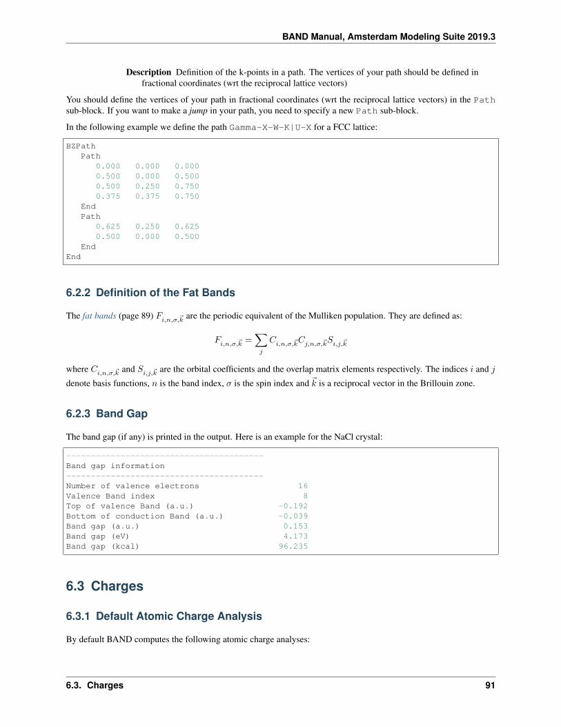
BAND Manual, Amsterdam Modeling Suite 2019.3
Description Definition of the k-points in a path. The vertices of your path should be defined infractional coordinates (wrt the reciprocal lattice vectors)
You should define the vertices of your path in fractional coordinates (wrt the reciprocal lattice vectors) in the Pathsub-block. If you want to make a jump in your path, you need to specify a new Path sub-block.
In the following example we define the path Gamma-X-W-K|U-X for a FCC lattice:
BZPathPath
0.000 0.000 0.0000.500 0.000 0.5000.500 0.250 0.7500.375 0.375 0.750
EndPath
0.625 0.250 0.6250.500 0.000 0.500
EndEnd
6.2.2 Definition of the Fat Bands
The fat bands (page 89) 𝐹𝑖,𝑛,𝜎,𝑘 are the periodic equivalent of the Mulliken population. They are defined as:
𝐹𝑖,𝑛,𝜎,𝑘 =∑𝑗
𝐶𝑖,𝑛,𝜎,𝑘𝐶𝑗,𝑛,𝜎,𝑘𝑆𝑖,𝑗,𝑘
where 𝐶𝑖,𝑛,𝜎,𝑘 and 𝑆𝑖,𝑗,𝑘 are the orbital coefficients and the overlap matrix elements respectively. The indices 𝑖 and 𝑗
denote basis functions, 𝑛 is the band index, 𝜎 is the spin index and is a reciprocal vector in the Brillouin zone.
6.2.3 Band Gap
The band gap (if any) is printed in the output. Here is an example for the NaCl crystal:
----------------------------------------Band gap information----------------------------------------Number of valence electrons 16Valence Band index 8Top of valence Band (a.u.) -0.192Bottom of conduction Band (a.u.) -0.039Band gap (a.u.) 0.153Band gap (eV) 4.173Band gap (kcal) 96.235
6.3 Charges
6.3.1 Default Atomic Charge Analysis
By default BAND computes the following atomic charge analyses:
6.3. Charges 91

BAND Manual, Amsterdam Modeling Suite 2019.3
• Hirshfeld Charges12
• Voronoi Deformation Charges (VDD, Voronoi Deformation Density)
• Mulliken Charges (note: not calculated for Spin-Orbit (page 24) calculations)
• CM5 (Charge Model 5)34
These atomic charges are printed to the output file and can be visualized using the ADFView GUI module.
A more detailed output of the atomic charges can be printed by specifying following print option (note: in Band 2017and previous versions this detailed output was printed by default):
Print AtomicChargesDetails
6.3.2 Bader Analysis (AIM)
The QTAIM (Quantum Theory of Atoms in Molecules), also known as Bader Analysis can be enabled in the Grid-BasedAIM input block:
GridBasedAIMEnabled [True | False]Iterations integerSmallDensity floatUseStartDensity [True | False]
End
GridBasedAIM
Type Block
Description Invoke the ultra fast grid based Bader analysis.
Enabled
Type Bool
Default value False
GUI name Bader (AIM): Atomic properties
Description Invoke the ultra fast grid based Bader analysis.
Iterations
Type Integer
Default value 40
Description The maximum number of steps that may be taken to find the nuclear attractor for agrid point.
SmallDensity
Type Float
1 F.L. Hirshfeld, Bonded-atom fragments for describing molecular charge densities, Theoretica Chimica Acta 44, 129 (1977)(https://doi.org/10.1007/BF00549096)
2 K.B. Wiberg and P.R. Rablen, Comparison of atomic charges derived via different procedures, Journal of Computational Chemistry 14, 1504(1993) (https://doi.org/10.1002/jcc.540141213)
3 A.V. Marenich, S.V. Jerome, C.J. Cramer, D.G. Truhlar, Charge Model 5: An Extension of Hirshfeld Population Analysis for the Accu-rate Description of Molecular Interactions in Gaseous and Condensed Phases, Journal of Chemical Theory and Computation 8, 527 (2012)(https://doi.org/10.1021/ct200866d)
4 C.A. Peeples and G. Schreckenbach, Implementation of the SM12 Solvation Model into ADF and Comparison with COSMO, Journal ofChemical Theory and Computation 12, 4033 (2016) (https://doi.org/10.1021/acs.jctc.6b00410)
92 Chapter 6. Analysis

BAND Manual, Amsterdam Modeling Suite 2019.3
Default value 1e-06
Description Value below which the density is ignored. This should not be chosen too smallbecause it may lead to unassignable grid points.
UseStartDensity
Type Bool
Default value False
Description Whether the analysis is performed on the startup density (True) or on the finaldensity (False).
AIMCriticalPointsEnabled [True | False]EqvPointsTol floatGridPadding floatGridSpacing float
End
AIMCriticalPoints
Type Block
Description Compute the critical points of the density (Atoms In Molecules). The algorithm startsfrom a regular mesh of points, and from each of these it walks towards its corresponding criticalpoint.
Enabled
Type Bool
Default value False
GUI name : Critical points and bond paths
Description Compute the critical points of the density (Atoms In Molecules). The algorithmstarts from a regular mesh of points, and from each of these it walks towards its correspondingcritical point.
EqvPointsTol
Type Float
Default value 0.27
Unit Bohr
Description If the distance between two critical points is smaller than this value, the two criticalpoints are considered to be the same point.
GridPadding
Type Float
Default value 0.7
Unit Bohr
Description How much extra space is added to the starting guess domain in the search for thecritical points
GridSpacing
Type Float
6.3. Charges 93

BAND Manual, Amsterdam Modeling Suite 2019.3
Default value 0.5
Unit Bohr
Description The distance between the initial trial points.
Note: The Bader (AIM) analysis is performed on the fitted density (see ZlmFit (page 56)). We advise to use a Good(or better) ZlmFit quality.
6.4 Fragments
A fragment feature is available albeit rather primitive. It allows for the analysis of the DOS in a fragment basis and forthe calculation of the deformation density with respect to fragment densities. A typical application is the periodicaladsorption of one or more molecules on a surface. For instance, consider periodic adsorption of hydrogen moleculesover a surface. First you calculate the free molecule in the same orientation as when adsorbed to the substrate. Sinceyou would like to use a molecular fragment, it makes sense to put the molecules far apart (large lattice spacing) andforce dispersion to be neglected (KSPACE 1). To use the fragment in the next run you need to rename the result file(“rkf”), to something like “frag.rkf”, see the example script discussed below or the example (page 204) covering thistopic.
FragmentAtomMapping # Non-standard block. See details.
...EndFilename stringLabels # Non-standard block. See details.
...End
End
Fragment
Type Block
Recurring True
Description Defines a fragment. You can define several fragments for a calculation.
AtomMapping
Type Non-standard block
Description Format ‘indexFragAt indexCurrentAt’. One has to associate the atoms of the frag-ment to the atoms of the current calculation. So, for each atom of the fragment the indexFra-gAt has to be associated uniquely to the indexCurrentAt for the current calculation.
Filename
Type String
Description Filename of the fragment. Absolute path or path relative to the executing directory.
Labels
Type Non-standard block
Description This gives the possibility to introduce labels for the fragment orbitals. See exam-ples.
94 Chapter 6. Analysis

BAND Manual, Amsterdam Modeling Suite 2019.3
Example:
Fragmentfilename test.rkfAtomMapping1 3 ! atom 1 of this fragment is assigned to third atom2 4 ! atom 2 of this fragment is assigned to fourth atom
EndLabelsSigmaSigma*Pi_xPi_yPi_x*Pi_y*
EndEnd
In this example the first six fragment orbitals will be labeled as stated in the body of this key. The remaining orbitalsare labeled by the default labeling system (e.g. 1/FO/5, etc.). The labels are used in combination with options likePrint Eigens and Print OrbPop. (See also Print OrbLabels). This key can be given once for eachfragment.
Tip: Specifying:
Print Eigens
for a calculation produces output concerning the eigen states, thereby providing a means to identify the eigen states(e.g. to be sigma, pi, et cetera). So, one can label the orbitals of a fragment according to this information.
6.5 Energy Decomposition Analysis
In BAND there are two fragment-based energy decomposition methods available: the periodic energy decompositionanalysis (PEDA)1 and the periodic energy decomposition analysis combined with the natural orbitals of chemicalvalency method (PEDA-NOCV)1.
6.5.1 Periodic Energy Decomposition Analysis (PEDA)
PEDA [True | False]
PEDA
Type Bool
Default value False
Description If present in combination with the fragment block, the decomposition of the interactionenergy between fragments is invoked.
1 M. Raupach and R. Tonner, A periodic energy decomposition analysis method for the investigation of chemical bonding in extended systems,The Journal of Chemical Physics 142, 194105 (2015) (https://doi.org/10.1063/1.4919943).
6.5. Energy Decomposition Analysis 95

BAND Manual, Amsterdam Modeling Suite 2019.3
If used in combination with the fragment keyblocks the decomposition of the interaction energy between fragmentsis invoked and the resulting energy terms (∆𝐸𝑖𝑛𝑡, ∆𝐸𝑑𝑖𝑠𝑝, ∆𝐸𝑃𝑎𝑢𝑙𝑖, ∆𝐸𝑒𝑙𝑠𝑡𝑎𝑡, ∆𝐸𝑜𝑟𝑏) presented in the output file.(See the example (page 216) or the tutorial)
Attention: In case of the error message “Fragments cannot be assigned by a simple translation!”, BAND doesonly allow for fragments which can be transformed to the structure in the PEDA calculation by a simple translation.So, a rotation is not allowed.
6.5.2 Periodic Energy Decomposition Analysis and natural orbitals of chemical va-lency (PEDA-NOCV)
PEDANOCV (block-type)
If present in combination with the fragment keyblocks and the PEDA key the decomposition of the orbital relaxationterm is performed. The binary result file will contain the information to plot NOCV Orbitals and NOCV deformationdensities (page 120).
See also:
• example (page 219)
• tutorial
• advanced tutorial
PEDANOCVEigvalThresh floatEnabled [True | False]
End
PEDANOCV
Type Block
Description Options for the decomposition of the orbital relaxation (pEDA).
EigvalThresh
Type Float
Default value 0.001
GUI name Use NOCVs with ev larger than
Description The threshold controls that for all NOCV deformation densities with NOCV eigen-values larger than EigvalThresh the energy contribution will be calculated and the respectivepEDA-NOCV results will be printed in the output
Enabled
Type Bool
Default value False
GUI name Perform PEDA-NOCV analysis
Description If true in combination with the fragment blocks and the pEDA key, the decomposi-tion of the orbital relaxation term is performed.
96 Chapter 6. Analysis

BAND Manual, Amsterdam Modeling Suite 2019.3
6.6 3D field visualization with BAND
With ADFView you can visualize three-dimensional fields from the results of a BAND Calculation (runkf file).
Following is a list of relevant fields, with a short explanation and illustrative pictures (from a simple non-periodic H2calculation). All fields are in atomic units (a.u.) (https://en.wikipedia.org/wiki/Atomic_units).
Total_Density (rho) The electronic density 𝜌(𝑟). The integral of the electronic density over the whole space (or, forperiodic systems, over the unit cell) equals the total number of electrons (valence + core).
Deformation density (rho(deformation)) The deformation density is the difference between total density 𝜌(𝑟) andreference density 𝜌reference(𝑟)
𝜌deformation(𝑟) = 𝜌(𝑟) − 𝜌reference(𝑟)
The reference density 𝜌reference(𝑟) is defined as the sum of densities of spherical spin-unrestricted isolated atoms.
The deformation density is electrically neutral, i.e. its integral over the whole space (or, for periodic systems,over the unit cell) is zero. Positive values of deformation density indicate density accumulation wrt isolatedatoms; negative values represent density depletion. In our H2 example, the deformation density shows howthere is electron accumulation in the bonding region between the two hydrogen atoms.
6.6. 3D field visualization with BAND 97

BAND Manual, Amsterdam Modeling Suite 2019.3
SCF_CoulombPot (v(coulomb)) The total Coulomb potential (nuclear + electronic potentials). BANDs conventionfor the Coulomb potential: the potential of positive charges (like nuclei) is negative, while the potential ofnegative charges (like electrons) is positive. In our example, the nuclear potential (negative) is larger than theelectronic potential (positive) in the region of space near the H2 molecule.
98 Chapter 6. Analysis

BAND Manual, Amsterdam Modeling Suite 2019.3
Note: The sign convention for potentials in BAND is the opposite to the ADF sign convention.
SCF_CoulombDeformation (v(coulomb/deformation)) The Coulomb potential originating from the (overall neu-tral) deformation density.
6.6. 3D field visualization with BAND 99
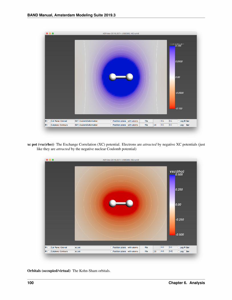
BAND Manual, Amsterdam Modeling Suite 2019.3
xc pot (vxc(rho)) The Exchange Correlation (XC) potential. Electrons are attracted by negative XC potentials (justlike they are attracted by the negative nuclear Coulomb potential)
Orbitals (occupied/virtual) The Kohn-Sham orbitals.
100 Chapter 6. Analysis
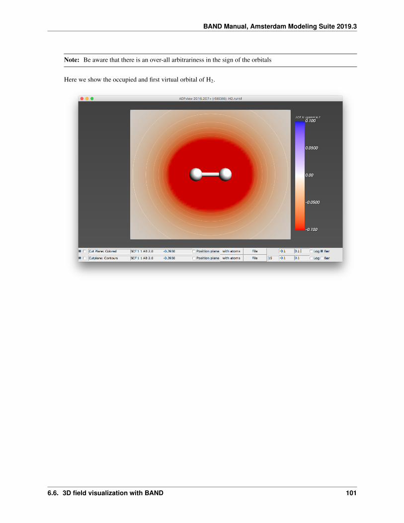
BAND Manual, Amsterdam Modeling Suite 2019.3
Note: Be aware that there is an over-all arbitrariness in the sign of the orbitals
Here we show the occupied and first virtual orbital of H2.
6.6. 3D field visualization with BAND 101

BAND Manual, Amsterdam Modeling Suite 2019.3
102 Chapter 6. Analysis
CHAPTER
SEVEN
ELECTRONIC TRANSPORT (NEGF)
See also:
BAND-NEGF GUI tutorial
Some examples are available in the $ADFHOME/examples/band directory and are discussed in the Examplessection.
Example: Main NEGF flavors (page 167)Example: NEGF with bias (page 173)
Note: In the BAND-GUI it is possible to choose between three NEGF methods (flavors):
Self consistent This is the internal BAND-NEGF implementation, which is described in this page.
Self consistent + align This is the internal BAND-NEGF implementation with an extra alignment-run (workflow step3a)
Non self consistent Computationally cheap method, equivalent to the DFTB-NEGF approach with 𝐻 and 𝑆 matrixelements computed by BAND (instead of DFTB).
7.1 Transport with NEGF in a nutshell
The Non-Equilibrium Green’s Functions formalism (NEGF) is a theoretical framework for modeling electron trans-port through nano-scale devices. Electron transport is treated as a one-dimensional coherent scattering process in the“scattering region” for electrons coming in from the electrodes:
103

BAND Manual, Amsterdam Modeling Suite 2019.3
Our goal is to compute the transmission function 𝑇 (𝐸), which describes the rate at which electrons of energy 𝐸are transferred from the left electrode to the right electrode by propagating through the scattering region. From thetransmission function we can calculate the electric current for given Bias Voltage 𝑉 applied between the electrodes:
𝐼(𝑉 ) =2𝑒
ℎ
∫ ∞
−∞𝑇 (𝐸, 𝑉 ) (𝑓(𝐸 − 𝜇𝐿) − 𝑓(𝐸 − 𝜇𝑅)) 𝑑𝐸
where 𝑓(𝐸) is the Fermi-Dirac distribution function for a given temperature, and 𝜇𝐿 (𝜇𝑅) is 𝜖𝐹 + 𝑒𝑉/2 (𝜖𝐹 − 𝑒𝑉/2),𝜖𝐹 being the Fermi energy of the electrodes.
The transmission function 𝑇 (𝐸) can be computed from the Green’s function of our system.
The Green’s function 𝐺(𝐸) of the scattering region is obtained solving the following equation:
(𝐸𝑆 −𝐻)𝐺(𝐸) = 𝐼
where 𝑆 is the overlap matrix, 𝐻 is the Hamiltonian and 𝐼 is the identity matrix. The Hamiltonian is composed asfollows (L, C and R denote the left lead, the central region and the right lead respectively):
𝐻 =
⎛⎝ 𝐻𝐿 + Σ𝐿 𝐻𝐿𝐶 0𝐻𝐿𝐶 𝐻𝐶 𝐻𝑅𝐶
0 𝐻𝑅𝐶 𝐻𝑅 + Σ𝑅
⎞⎠The two self-energies Σ𝐿 and Σ𝑅 model the two semi-infinite electrodes.
The transmission function 𝑇 (𝐸) can be calculated from the Green’s function 𝐺(𝐸) and the so-called broadeningmatrices Γ𝐿(𝐸) and Γ𝑅(𝐸):
𝑇 (𝐸) = 𝑇𝑟[𝐺(𝐸)Γ𝑅(𝐸)𝐺(𝐸)Γ𝐿(𝐸)]
The broadening matrix being
Γ𝐿(𝐸) = −2ℑΣ𝐿(𝐸)
104 Chapter 7. Electronic Transport (NEGF)

BAND Manual, Amsterdam Modeling Suite 2019.3
7.1.1 Self consistency
The density matrix is determined self consistently1:
𝑃in → 𝐻𝐾𝑆shifts−→ 𝐻aligned + Σ𝐿(𝐸) + Σ𝑅(𝐸) → 𝐺(𝐸)
∫𝑑𝑒
−→ 𝑃out
From a guess of the density matrix the corresponding KS Hamiltonian is calculated. This Hamiltonian is aligned, andthen the NEGF Hamiltonian in the complex plane is constructed by adding the self energies, representing the influenceof the electrodes. From the resulting Green’s function a new density matrix follows.
From the difference between input and output density a next input is guessed. This is repeated until the input andoutput densities converge.
For the alignment of the Hamiltonian there are two shifts. The first shift aligns the potential in the leads to theelectrodes.
shift 1 =1
𝑛
𝑛∑i in lead
𝐻𝑇𝐵𝑖𝑖 −𝐻𝐾𝑆
𝑖𝑖
𝑆𝑖𝑖
The second and usually smaller shift results from the alignment run. A shift ∆ is applied globally
𝐻aligned𝑖𝑗 = 𝐻𝑖𝑗 + ∆𝑆𝑖𝑗
7.1.2 Contour integral
Without bias the density matrix follows from
𝑃 (𝜇) = − 1
𝜋
∫ ∞
−∞𝑑𝑒 𝑓(𝑒, 𝜇) ℑ𝐺(𝑒)
As the Green’s function is singular on the real axis we add a small imaginary value (eta) to the energy. Still, theintegrand will be very wild function, and it is numerically better to do a contour integral instead.
Fig. 7.1: Figure: BAND uses a rectangular contour in the complex energy plane to integrate the (integrand of the)density matrix. The integrand also needs to be evaluated in the enclosed FD poles (three in this picture).
1 C. J. O. Verzijl and J. M. Thijssen DFT-Based Molecular Transport Implementation in ADF/BAND, J. Phys. Chem. C, 2012, 116 (46), pp24393–24412 (https://doi.org/10.1021/jp3044225).
7.1. Transport with NEGF in a nutshell 105
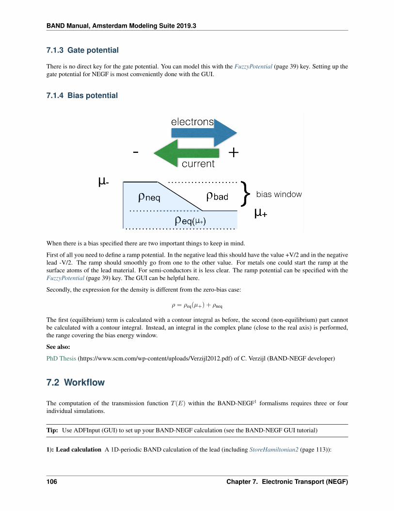
BAND Manual, Amsterdam Modeling Suite 2019.3
7.1.3 Gate potential
There is no direct key for the gate potential. You can model this with the FuzzyPotential (page 39) key. Setting up thegate potential for NEGF is most conveniently done with the GUI.
7.1.4 Bias potential
When there is a bias specified there are two important things to keep in mind.
First of all you need to define a ramp potential. In the negative lead this should have the value +V/2 and in the negativelead -V/2. The ramp should smoothly go from one to the other value. For metals one could start the ramp at thesurface atoms of the lead material. For semi-conductors it is less clear. The ramp potential can be specified with theFuzzyPotential (page 39) key. The GUI can be helpful here.
Secondly, the expression for the density is different from the zero-bias case:
𝜌 = 𝜌eq(𝜇+) + 𝜌neq
The first (equilibrium) term is calculated with a contour integral as before, the second (non-equilibrium) part cannotbe calculated with a contour integral. Instead, an integral in the complex plane (close to the real axis) is performed,the range covering the bias energy window.
See also:
PhD Thesis (https://www.scm.com/wp-content/uploads/Verzijl2012.pdf) of C. Verzijl (BAND-NEGF developer)
7.2 Workflow
The computation of the transmission function 𝑇 (𝐸) within the BAND-NEGF1 formalisms requires three or fourindividual simulations.
Tip: Use ADFInput (GUI) to set up your BAND-NEGF calculation (see the BAND-NEGF GUI tutorial)
1): Lead calculation A 1D-periodic BAND calculation of the lead (including StoreHamiltonian2 (page 113)):
106 Chapter 7. Electronic Transport (NEGF)
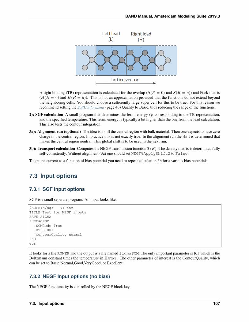
BAND Manual, Amsterdam Modeling Suite 2019.3
A tight binding (TB) representation is calculated for the overlap (𝑆(𝑅 = 0) and 𝑆(𝑅 = 𝑎)) and Fock matrix(𝐻(𝑅 = 0) and 𝐻(𝑅 = 𝑎)). This is not an approximation provided that the functions do not extend beyondthe neighboring cells. You should choose a sufficiently large super cell for this to be true. For this reason werecommend setting the SoftConfinement (page 46) Quality to Basic, thus reducing the range of the functions.
2): SGF calculation A small program that determines the fermi energy 𝜖𝐹 corresponding to the TB representation,and the specified temperature. This fermi energy is typically a bit higher than the one from the lead calculation.This also tests the contour integration.
3a): Alignment run (optional) The idea is to fill the central region with bulk material. Then one expects to have zerocharge in the central region. In practice this is not exactly true. In the alignment run the shift is determined thatmakes the central region neutral. This global shift is to be used in the next run.
3b): Transport calculation Computes the NEGF transmission function 𝑇 (𝐸). The density matrix is determined fullyself-consistently. Without alignment (3a) one should set NEGF%ApplyShift2 to False.
To get the current as a function of bias potential you need to repeat calculation 3b for a various bias potentials.
7.3 Input options
7.3.1 SGF Input options
SGF is a small separate program. An input looks like:
$ADFBIN/sgf << eorTITLE Test for NEGF inputsSAVE SIGMASURFACEGF
SCMCode TrueKT 0.001ContourQuality normal
ENDeor
It looks for a file RUNKF and the output is a file named SigmaSCM. The only important parameter is KT which is theBoltzmann constant times the temperature in Hartree. The other parameter of interest is the ContourQuality, whichcan be set to Basic,Normal,Good,VeryGood, or Excellent.
7.3.2 NEGF Input options (no bias)
The NEGF functionality is controlled by the NEGF block key.
7.3. Input options 107
BAND Manual, Amsterdam Modeling Suite 2019.3
NEGFLeadFile stringSGFFile stringContourQuality [basic | normal | good | verygood]EMin floatEMax floatNE integer
End
NEGF
Type Block
Description Options for the NEGF (non-equilibrium green function) transport calculation.
LeadFile
Type String
Default value
Description File containing the tight binding representation of the lead.
SGFFile
Type String
Default value
Description The result from the SGF program. Contains the Fermi energy of the lead.
ContourQuality
Type Multiple Choice
Default value good
Options [basic, normal, good, verygood]
Description The density matrix is calculated numerically via a contour integral. Changing thequality influences the number of points. This influences a lot the performance.
EMin
Type Float
Default value -5.0
Unit eV
Description The minimum energy for the transmission grid (with respect to the Fermi level ofthe lead)
EMax
Type Float
Default value 5.0
Unit eV
Description The maximum energy for the transmission grid (with respect to the Fermi level ofthe lead)
NE
Type Integer
108 Chapter 7. Electronic Transport (NEGF)

BAND Manual, Amsterdam Modeling Suite 2019.3
Default value 100
Description The number of energies for the transmission energy grid.
The following are expert / technical options:
NEGFCheckOverlapTol floatEta floatApplyShift1 [True | False]ApplyShift2 [True | False]YContourInt floatDEContourInt float
End
NEGF
Type Block
Description Options for the NEGF (non-equilibrium green function) transport calculation.
CheckOverlapTol
Type Float
Default value 0.01
Description BAND checks how well the TB overlap matrix S(R=0) represents the overlap ma-trix in the lead region. Elements corresponding to the outer layer are neglected, becausewhen using a frozen core they have bigger errors.
Eta
Type Float
Default value 1e-05
Description Small value used for the contour integral: stay at least this much above the real axis.This value is also used for the evaluation of the Transmission and dos.
ApplyShift1
Type Bool
Default value True
Description Apply the main shift, obtained from comparing matrix elements in the leads withthose from the tight-binding run. Strongly recommended.
ApplyShift2
Type Bool
Default value True
Description Apply the smaller alignment shift. This requires an extra alignment run. Usuallythis shift is smaller.
YContourInt
Type Float
Default value 0.3
Description The density is calculated via a contour integral. This value specifies how far abovethe real axis the (horizontal part of the) contour runs. The value is rounded in such a waythat it goes exactly halfway between two Fermi poles. There is a trade off: making it bigger
7.3. Input options 109

BAND Manual, Amsterdam Modeling Suite 2019.3
makes the integrand more smooth, but the number of enclosed poles increases. For lowtemperatures it makes sense to lower this value, and use a smaller deContourInt.
DEContourInt
Type Float
Default value -1.0
Description The energy interval for the contour grid. Defaults depends on the contour quality
7.3.3 NEGF Input options (with bias)
With a bias potential there are some extra keys.
NEGFBiasPotential floatNonEqDensityMethod integerBoundOccupationMethod integerYRealaxisInt floatDERealAxisInt float
End
NEGF
Type Block
Description Options for the NEGF (non-equilibrium green function) transport calculation.
BiasPotential
Type Float
Default value 0.0
Description Apply a bias potential (atomic units). Can be negative. One has to specify the ramppotential with the FuzzyPotential key. This is mostly conveniently done with the GUI.
NonEqDensityMethod
Type Integer
Default value 1
Description See text.
BoundOccupationMethod
Type Integer
Default value 1
Description See text. Only relevant with NonEqDensityMethod equal 2 or 3.
YRealaxisInt
Type Float
Default value 1e-05
Description The non-Equilibrium density is calculated near the real axis.
DERealAxisInt
Type Float
110 Chapter 7. Electronic Transport (NEGF)

BAND Manual, Amsterdam Modeling Suite 2019.3
Default value -1.0
Description The energy interval for the real axis grid. Defaults depends on the contour quality.
NonEqDensityMethod Let us introduce some terms2. First of all the total density in the bias window (ignoringoccupation)
𝐷 =1
2𝜋
∫𝐴 (𝑓− − 𝑓+)
And then there are the side resolved densities
𝐷+/− =1
2𝜋
∫𝐴+/− (𝑓− − 𝑓+)
The issue here is that the side resolved densities do not sum to the total one
𝐷 = 𝐷+ + 𝐷− + 𝐷bound states
The NonEqDensityMethod is about how these integrals are calculated . With option 1, or 2 a contour integral isused for D: they are essentially the same. However, when choosing option 2, you can choose a BoundOccupa-tionMethod, leading to other physics. If set to 3, the total density in the bias window (D) will be calculated nearthe real axis: this way one avoids the possibility of a negative nr. of bound states (deviating from2).
BoundOccupationMethod Only relevant with NonEqDensityMethod equal 2 or 3. If set to one, the density ofbound states (ignoring occupation) is simply multiplied by a half. If set to two, atoms closer to the negativelead will get a higher occupation2. Atoms coupled to the right lead will have a low occupation. For this werecommend setting NonEqDensityMethod to 3, to avoid a possible negative number of bound states.
Fig. 7.2: Figure: The non-equilibrium density consists of three parts: the left and right parts (𝜌-/neq and 𝜌+/neq) andthe bound states (𝜌bound). We want to know the occupied part.
Setting the method BoundOccupationMethod to 1, leads to
𝜌 = 𝜌(𝜇+) + 𝜌-/neq +1
2𝜌bound
By setting the method to 2, each atom gets its own weight in the density matrix
𝜌𝑖𝑗 = 𝜌𝑖𝑗(𝜇+) + 𝜌-/neq +√𝑤𝑖𝑤𝑗𝜌
bound𝑖𝑗
with2
𝑤𝑖 =Tr[𝐷−]𝑖
Tr[𝐷−]𝑖 + Tr[𝐷+]𝑖
2 Rui Li, Jiaxing Zhang, Shimin Hou, Zekan Qian, Ziyong Shen, Xingyu Zhao, Zengquan Xue, A corrected NEGF + DFT approach forcalculating electronic transport through molecular devices: Filling bound states and patching the non-equilibrium integration, Chemical Physics336 (2007) 127-135 (https://doi.org/10.1016/j.chemphys.2007.06.011).
7.3. Input options 111

BAND Manual, Amsterdam Modeling Suite 2019.3
These weights are the same for all functions on an atom. The intended effect is: bound states that are coupledmore strongly to the negative electrode get a higher occupation than the ones that are coupled more strongly tothe positive electrode.
To summarize here are three reasonable settings
NonEqDensityMethod BoundOccupationMethod intention1 1 Multiply the bound states with a half2 2 Occupy bound states with atom-resolved 𝑤𝑖
3 2 ... and prevent a negative nr. of bound states
To get the current from a calculation you can use adfprep:
$ADFBIN/adfreport RUNKF 'NEGF%current'
7.3.4 NEGF Input options (alignment)
For the (optional) alignment run there are some extra keys.
NEGFDoAlignment [True | False]Alpha floatAlignChargeTol floatCDIIS [True | False]
End
NEGF
Type Block
Description Options for the NEGF (non-equilibrium green function) transport calculation.
DoAlignment
Type Bool
Default value False
Description Set this to True if you want to do an align run. Between the leads there should belead material. The GUI can be of help here.
Alpha
Type Float
Default value 1e-05
Description A charge error needs to be translated in a potential shift. DeltaV = alpha * DeltaQ
AlignChargeTol
Type Float
Default value 0.1
Description In an alignment run you want to get the number of electrons in the center right. Thisnumber specifies the criterion for that.
CDIIS
Type Bool
Default value False
112 Chapter 7. Electronic Transport (NEGF)

BAND Manual, Amsterdam Modeling Suite 2019.3
Description Make the normal DIIS procedure aware of the align charge error
7.4 Troubleshooting
The self consistent approach, unique to BAND, may be difficult to converge. If this is true for the alignment run it canbe decided to skip this run. For the final transport run, here are some tips / considerations.
• Use a SZ basis for the metal atoms
• Restart (the density matrix) from the result of a smaller (such as the SZ) basis. (See “Save (page 122) Density-Matrix” and the Restart (page 115) key)
• Restart (the density matrix) from the result obtained with a smaller bias (only relevant for calculations with biaspotential).
• Setting NEGF%BoundOccupationMethod to 2 (and NEGF%NonEqDensityMethod to 3) might help. Note thatthis affects the physics: you are differently occupying the bound states.
• Use a better NEGF%ContourQuality (there comes a computational price tag with this).
If everything fails it is possible to use BAND in a non-self consistent way, similar to the way DFTB-NEGF works.This option is available via the GUI.
7.5 Miscellaneous remarks on BAND-NEGF
• You should make sure that your results are converged with respect to the number of lead repetitions; the resultsshould not change significantly if you increase the number of lead repetitions.
• It’s good practice to include at least one lead repetition in the central region.
7.5.1 Store tight-binding Hamiltonian
Let us consider a Fourier transformation of a 1D Bloch matrix
𝑆(𝑅 = 𝑛𝑎) =
∫𝑘
𝑒−𝑖𝑘𝑅𝑆(𝑘)
In (the tight-binding) case that the functions do not extend beyond the neighboring cells only S(R=0) and S(R=a) arenonzero. (And S(R=-a) is equivalent to S(R=a))
StoreHamiltonian2 [True | False]
StoreHamiltonian2
Type Bool
Default value False
Description determine the tight-binding representation of the overlap an fock matrix. Used for (atleast) NEGF.
Adding StoreHamiltonian2 to the input cause band to determine the tight-binding representation of the overlap an fockmatrix. Currently this only works for 1D periodic systems. For the overlap matrix you will get two parts. The first𝑆(𝑅 = 0) is the (symmetric) overlap matrix of atoms in the unit cell. The second 𝑆(𝑅 = 𝑎) is a non symmetric matrixdescribing the coupling of functions in the central cell with functions in its right neighboring cell. On the RUNKFfile you will find the TB representations of the overlap and Hamiltonian stored in the ‘Matrices’ section as “S(R)” and“H(R)”, being dimensioned (nBas,nBas,2).
7.4. Troubleshooting 113

BAND Manual, Amsterdam Modeling Suite 2019.3
114 Chapter 7. Electronic Transport (NEGF)

CHAPTER
EIGHT
EXPERT OPTIONS
8.1 Restarts
The main results of a BAND calculation are stored in the rkf file. If you save this file you can use it to restart yourcalculation. The input for the restart calculation is essentially the same, except for some extra keys, like Restart,Grid, and DensityPlot.
Plots of the density (and many other symmetric properties) can can be obtained with the key DensityPlot. Densityand orbital plot restarts require the specification of the Grid key. With the subkey SCF you can start the SCFprocedure with the last solution from the restart file. This can be useful if the SCF did not converge or if you want tocompute some post-SCF properties (e.g. the DOS (page 85) or the band structure (page 89)). Similarly, a geometryoptimization can be restarted with the subkey GeometryOptimization You can use the geometry of a previouscalculation.
Usually the input for a restarted job is the same as for the original calculation, with some extra options, described inthis section.
Some examples are available in the $ADFHOME/examples/band directory and are discussed in the Examplessection.
Example: Restart SCF for properties calculation (page 163)Example: Restart the SCF (page 159)Example: Properties on a grid (page 165)
8.1.1 Restart key
RestartFile stringSCF [True | False]DensityPlot [True | False]OrbitalPlot [True | False]NOCVdRhoPlot [True | False]NOCVOrbitalPlot [True | False]UseDensityMatrix [True | False]
End
Restart
Type Block
Description Tells the program that it should restart with the restart file, and what to restart.
File
Type String
115

BAND Manual, Amsterdam Modeling Suite 2019.3
Default value
Description Name of the restart file.
SCF
Type Bool
Default value False
GUI name Restart: SCF
Description Continue the SCF procedure using the orbital coefficients and occupations from therestart file.
DensityPlot
Type Bool
Default value False
Description Goes together with the DensityPlot block and Grid blocks
OrbitalPlot
Type Bool
Default value False
Description Goes together with the OrbitalPlot and Grid
NOCVdRhoPlot
Type Bool
Default value False
Description Goes together with the NOCVdRhoPlot and Grid blocks.
NOCVOrbitalPlot
Type Bool
Default value False
Description Goes together with the NOCVOrbitalPlot and Grid blocks.
UseDensityMatrix
Type Bool
Default value False
Description If set to True: For restarting the SCF the density matrix will be used. Requires youto set ‘Save DensityMatrix’ in the previous run.
8.1.2 Grid
The Grid block is used for restart options OrbitalPlot, DensityPlot, NOCVOrbitalPlot andNOCVdRhoPlot. There are two ways to define your grid. The most easy way is to use the Type key, which au-tomatically generates a grid around the atoms in the unit cell:
116 Chapter 8. Expert Options
BAND Manual, Amsterdam Modeling Suite 2019.3
GridType [coarse | medium | fine]
End
Grid
Type Block
Description Options for the regular grid used for plotting (e.g. density plot). Used ICW the restartoption.
Type
Type Multiple Choice
Default value coarse
Options [coarse, medium, fine]
Description The default regular grids.
One alternative is to specify everything by hand via the ‘UserDefined’ sub-block.
GridUserDefined # Non-standard block. See details.
...End
End
Grid
Type Block
Description Options for the regular grid used for plotting (e.g. density plot). Used ICW the restartoption.
UserDefined
Type Non-standard block
Description Once can define the regular grid specification in this block. See example.
The following input would create a cube from (-1,-1,-1) to (1,1,1):
GridUserDefined
-1 -1 -1 ! Starting point1 0 0 0.1 ! vec1 and dvec10 1 0 0.1 ! vec2 and dvec20 0 1 0.1 ! vec3 and dvec320 20 20 ! nr. of steps along three directions
EndEnd
One can also specify a text file from which the grid is imported:
GridFileName string
End
Grid
Type Block
8.1. Restarts 117

BAND Manual, Amsterdam Modeling Suite 2019.3
Description Options for the regular grid used for plotting (e.g. density plot). Used ICW the restartoption.
FileName
Type String
Default value
Description Read in the grid from a file. The file format of the grid is: three numbers per line(defining the x, y and z coordinates of the points).
8.1.3 Plots of the density, potential, and many more properties
DensityPlot # Non-standard block. See details....
End
DensityPlot
Type Non-standard block
Description Plots of the density. Goes together with the Restart%DensityPlot and Grid keys.
The DensityPlot block goes together with the Restart%DensityPlot and Grid keys. Example input:
...Restart
File my_file.rkfDensityPlot
End
GridType Coarse
End
DensityPlotrho(fit)vxc[rho]
End...
After such a run you get a TAPE41 file that you should rename to my.t41, and view with ADFview. The most commonproperties to plot are:
• rho(fit) The fitted density.
• v(coulomb) The Coulomb potential.
• vxc[rho(fit)] the XC potential (using the fitted density)
• vxc[rho] XC potential of the exact density
• rho The density
• |gradRho| The norm of the gradient of the density
• tau The symmetric kinetic energy density
• LDOS The local density of states. (See LDOS key (page 121))
• elf[rho] The electron localization function
118 Chapter 8. Expert Options
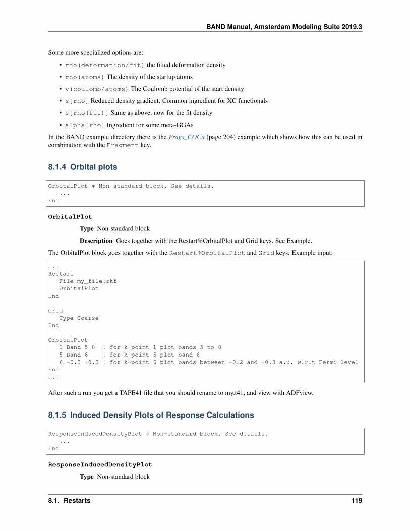
BAND Manual, Amsterdam Modeling Suite 2019.3
Some more specialized options are:
• rho(deformation/fit) the fitted deformation density
• rho(atoms) The density of the startup atoms
• v(coulomb/atoms) The Coulomb potential of the start density
• s[rho] Reduced density gradient. Common ingredient for XC functionals
• s[rho(fit)] Same as above, now for the fit density
• alpha[rho] Ingredient for some meta-GGAs
In the BAND example directory there is the Frags_COCu (page 204) example which shows how this can be used incombination with the Fragment key.
8.1.4 Orbital plots
OrbitalPlot # Non-standard block. See details....
End
OrbitalPlot
Type Non-standard block
Description Goes together with the Restart%OrbitalPlot and Grid keys. See Example.
The OrbitalPlot block goes together with the Restart%OrbitalPlot and Grid keys. Example input:
...Restart
File my_file.rkfOrbitalPlot
End
GridType Coarse
End
OrbitalPlot1 Band 5 8 ! for k-point 1 plot bands 5 to 85 Band 6 ! for k-point 5 plot band 66 -0.2 +0.3 ! for k-point 6 plot bands between -0.2 and +0.3 a.u. w.r.t Fermi level
End...
After such a run you get a TAPE41 file that you should rename to my.t41, and view with ADFview.
8.1.5 Induced Density Plots of Response Calculations
ResponseInducedDensityPlot # Non-standard block. See details....
End
ResponseInducedDensityPlot
Type Non-standard block
8.1. Restarts 119

BAND Manual, Amsterdam Modeling Suite 2019.3
Description Goes together with Restart%ResponseInducedDensityPlot and Grid.
ResponseInducedDensityPlot (block-type) The ResponseInducedDensityPlot block goes togetherwith the Restart%ResponseInducedDensityPlot and Grid keys. In the BAND example directory thereis the TD-CDFT for MoS2 Monolayer (page 191) example that shows how this can be used. Example input:
...Restart
File my_file.rkfResponseInducedDensityPlot
End
GridType Coarse
End
ResponseInducedDensityPlotXCOMPONENT 5 8 ! plot x component of induced densities
! for frequencies number 5 to 8YCOMPONENT 6 ! plot y component of induced densities
! for frequency number 6ZCOMPONENT 1 ! plot z component of induced densities
! for frequency number 1End...
After such a run you get a TAPE41 file that you should rename to my.t41, and view with ADFview.
Attention: The plotting capability works only with response calculation RUNKF files based on the NewResponse(page 73) method!
8.1.6 NOCV Orbital Plots
NOCVOrbitalPlot # Non-standard block. See details....
End
NOCVOrbitalPlot
Type Non-standard block
Description Goes together with the Restart%NOCVOrbitalPlot and Grid keys. See example.
The NOCVOrbitalPlot blockg oes together with the Restart%NOCVOrbitalPlot and Grid keys. See examplePEDANOCV_MgO+CO (page 219). Example input:
...Restart
File my_file.rkfNOCVOrbitalPlot
End
GridType Coarse
End
120 Chapter 8. Expert Options

BAND Manual, Amsterdam Modeling Suite 2019.3
NOCVOrbitalPlot1 Band 5 8 ! for k-point 1 plot NOCV Orbitals 5 to 8
End...
After such a run you get a TAPE41 file that you should rename to my.t41, and view with ADFview.
8.1.7 NOCV Deformation Density Plots
NOCVdRhoPlot # Non-standard block. See details....
End
NOCVdRhoPlot
Type Non-standard block
Description Goes together with the Restart%NOCVdRhoPlot and Grid keys. See example.
The NOCVdRhoPlot blockg oes together with the Restart%NOCVdRhoPlot and Grid keys. See examplePEDANOCV_MgO+CO (page 219). Example input:
...Restart
File my_file.rkfNOCVdRhoPlot
End
GridType Coarse
End
NOCVdRhoPlot1 Band 5 8 ! for k-point 1 plot NOCV deformation densities 5 to 8
End...
After such a run you get a TAPE41 file that you should rename to my.t41, and view with ADFview.
8.1.8 LDOS (STM)
LDOSDeltaNeg floatDeltaPos floatShift float
End
LDOS
Type Block
Description Local Density-Of-States information. This can be used to generate STM images in theTersoff-Hamann approximation (see https://doi.org/10.1103/PhysRevB.31.805)
DeltaNeg
Type Float
8.1. Restarts 121

BAND Manual, Amsterdam Modeling Suite 2019.3
Default value 0.0001
Unit Hartree
Description Lower bound energy (Shift-DeltaNeg)
DeltaPos
Type Float
Default value 0.0001
Unit Hartree
Description Upper bound energy (Shift+DeltaPos)
Shift
Type Float
Default value 0.0
Unit Hartree
Description The energy bias with respect to the Fermi level.
The local density of states is integrated over the resulting interval. Example of an LDOS restart:
RestartFile my_file.rkfDensityPlot
End
GridType Coarse
End
DensityPlotLDOS
End
LDOSShift 0.1DeltaNeg 0.001DeltaPos 0.0
End
According to this example, we restart from the result file of a previous calculation. The calculation will generate a fileTAPE41 which can be viewed with ADFview. (Rename the file to my.t41)
See also Restart (page 115), and DensityPlot (page 118).
8.1.9 Save
Save string
Save
Type String
Recurring True
122 Chapter 8. Expert Options

BAND Manual, Amsterdam Modeling Suite 2019.3
Description Save scratch files or extra data that would be otherwise deleted at the end of the calcu-lation. e.g. ‘TAPE10’ (containing the integration grid) or ‘DensityMatrix’
8.2 Symmetry
The symmetry of the system is automatically detected. Normally the symmetry of the initial system is maintained.One can lower the symmetry with the Symmetry key. In such cases the keyword POTENTIALNOISE can force thesolution away from the initial symmetry.
Whether or not symmetry should be used can be controlled vial the UseSymmetry key
UseSymmetry [True | False]
UseSymmetry
Type Bool
Default value True
Description Whether or not to exploit symmetry during the calculation.
One can also select a sub set of symmetry operators:
SubSymmetry integer_list
SubSymmetry
Type Integer List
Description The indices of the symmetry operators to maintain.
To get the indices of the symmetry operators, you should first run the calculation with the following options added toyour input:
print symmetrystopafter gemtry
and then you look in the output for (here the first four operators are listed)
::
64 SYMMETRY OPERATORS:
NO MATRIX TRANSL AXIS DET ROTATION--------------------------------------------------------------------------
1) 1.000 0.000 0.000 0.000 0.000 1.0 10.000 1.000 0.000 0.000 0.0000.000 0.000 1.000 0.000 1.000
2) 1.000 0.000 0.000 0.000 0.000 1.0 10.000 1.000 0.000 5.400 0.0000.000 0.000 1.000 0.000 1.000
3) 1.000 0.000 0.000 5.400 0.000 1.0 10.000 1.000 0.000 0.000 0.0000.000 0.000 1.000 0.000 1.000
8.2. Symmetry 123

BAND Manual, Amsterdam Modeling Suite 2019.3
4) 1.000 0.000 0.000 5.400 0.000 1.0 10.000 1.000 0.000 5.400 0.0000.000 0.000 1.000 0.000 1.000
from this list you should select the desired operators and use that in your final calculation, for example:
SubSymmetry 1 7 21 31
8.2.1 Symmetry breaking for SCF
PotentialNoise float
PotentialNoise
Type Float
Default value 0.0001
Description The initial potential for the SCF procedure is constructed from a sum-of-atoms density.Added to this is some small noise in the numerical values of the potential in the points of theintegration grid. The purpose of the noise is to help the program break the initial symmetry,if that would lower the energy, by effectively inducing small differences between (initially)degenerate orbitals.
8.3 Advanced Occupation Options
By default the levels are occupied according to the aufbau principle. In some cases it is possible to create holes belowthe Fermi level or uneven occupation for alpha and beta electrons with the Occupations (Γ-only) and alternativelythe EnforcedSpinPolarization (for an arbitrary number of k-points) key.
Occupations # Non-standard block. See details....
End
Occupations
Type Non-standard block
Description Allows one to input specific occupations numbers. Applies only for calculations thatuse only one k-point (i.e. pseudo-molecule calculations). See example.
Example:
OCCUPATIONS1 occupations_alpha // occupations_beta
End
• occupations_beta and the separating double slash (//) must not be used in a spin-restricted calculation.
• occupations_alpha/beta is a sequence of values assigned to the states (‘bands’) in energy ordering.
ElectronHoleBandIndex integerSpinIndex integer
End
124 Chapter 8. Expert Options

BAND Manual, Amsterdam Modeling Suite 2019.3
ElectronHole
Type Block
Description Allows one to specify an occupied band which shall be depopulated, where the elec-trons are then moved to the Fermi level. For a spin-restricted calculation 2 electrons are shiftedand for a spin-unrestricted calculation only one electron is shifted.
BandIndex
Type Integer
Description Which occupied band shall be depopulated.
SpinIndex
Type Integer
Description Defines the spin of the shifted electron (1 or 2).
See the example Si_ElectronHole (page 231)
8.3. Advanced Occupation Options 125

BAND Manual, Amsterdam Modeling Suite 2019.3
126 Chapter 8. Expert Options

CHAPTER
NINE
TROUBLESHOOTING
9.1 Recommendations
9.1.1 Model Hamiltonian
Relativistic model
By default we do not use relativistic effects. The best approximation is to use spin-orbit coupling, however that iscomputationally very expensive. The scalar relativistic option comes for free, and for light elements will give verysimilar results as non-relativistic theory, and for heavy ones better results w. r. t. experiment. We recommend toalways use this (scalar ZORA). To go beyond to the spin-orbit level can be important when there are heavy elementswith p valence electrons. Also the band gap appears quite sensitive for the spin-orbit effect.
XC functional
The default functional is the LDA, that gives quite good geometries but terrible bonding energies. GGA functionals areusually better at bonding energies, and among all possibilities the PBE is a common choice. Using a GGA is not a lotmore expensive than using plain LDA. For the special problem of band gaps there are a number Model Hamiltonians(page 11) available (eg. TB-mBJ and GLLC-SC). The Unrestricted (page 24) option will be needed when the systemis not closed shell. For systems interacting through dispersion interactions it is advised to use the Grimme corrections(page 14). Unfortunately there is no clear-cut answer to this problem, and one has to try in practice what works best.
9.1.2 Technical Precision
See also:
• Which basis set should I use? (page 42)
• Recommendations for k-space (page 52)
The easiest way to control the technical precision is via the NumericalQuality (page 41) key. One can also indepen-dently tweak the precision of specific technical aspects, e.g.:
BeckeGridQuality Good ! tweak the grid
EndKSpace
Quality Good ! tweak the k-space gridEndZlmFit
Quality Normal ! tweak the density fit
127

BAND Manual, Amsterdam Modeling Suite 2019.3
EndSoftConfiment
Quality Basic ! tweak the radial confinement of basis functionsEnd
Here are per issue hints for when to go for a better quality (but it is by no means complete)
• BeckeGrid: Increase quality if there are geometry convergence problems. Also negative frequencies can becaused by an inaccurate grid.
• KSpace: Increase quality for metals
• ZlmFit: Increase quality if the SCF does not converge.
• SoftConfinment: Increase quality for weakly bonded systems, such as layered materials
9.1.3 Performance
The performance is influenced by the model Hamiltonian and basis set, discussed above. Here follow more technicaltips.
Reduced precision
One of the simplest things to try is to run your job with NumericalQuality Basic. For many systems this will work well,and it can be used for instance to pre-optimize a geometry. However, it can also cause problems such as problematicSCF convergence, geometry optimization, or simply bad results. See above how to tweak more finely the TechnicalPrecision (page 127).
Memory usage
Another issue that is the choice CPVector (say the vector length of you machine) and the number of k-points processedtogether during the calculation of the parameters. In the output you see the used value
========================== Numerical Integration ==========================
TOTAL NR. OF POINTS 4738BLOCK LENGTH 256NR. OF BLOCKS 20MAX. NR. OF SYMMETRY UNIQUE POINTS PER BLOCK 35NR. OF K-POINTS PROCESSED TOGETHER IN BASPNT 5NR. OF SYMMETRY OPERATORS (REAL SPACE) 48SYMMETRY OPERATORS IN K-SPACE 48
If you want to change the default settings you can specify the CPVector and KGRPX keywords. The optimal combi-nation depends on the calculation, on the machine. Example
CPVector 512KGRPX 3
Note: bigger is not necessarily better.
128 Chapter 9. Troubleshooting

BAND Manual, Amsterdam Modeling Suite 2019.3
Reduced basis set
When starting work on a large unit cell it is wise to start with a DZ basis. With such a basis, one can test for instancethe quality of the k-space integration. However, for most properties, the DZ basis is probably not very accurate. Youcan next go for the DZP (if available) or TZP basis set, but that may be a bit of overkill.
Frozen core for 5d elements
The standard basis sets TZ2P are not optimal for third-row transition elements. Sometimes you need to relax the frozencore dependency criterion
Dependency Core=0.8 ! The frozen core overlap may not be exactly 1
9.2 Troubleshooting
9.2.1 SCF does not converge
Some systems are more difficult to converge than others. A Pd slab for instance is easier to converge than an Fe slab.Generally, what you do in a problematic case is to go for more conservative settings. The two main option are todecrease SCF%Mixing and/or DIIS%Dimix.
SCFMixing 0.05 ! more conservative mixing
End
DiisDiMix 0.1 ! also more conservative strategy for DIIS procedureAdaptable false ! disable automatic changing of dimix
End
ConvergenceDegenerate Default ! For most calculations this is quite a good idea anyway
End
An other option is to first run the system with a SZ basis, which may be easier to converge. Then you can Restart(page 115) the SCF with a larger basis set from this result.
Sometimes SCF convergence problems are caused by bad precision. An indication of this is when there are many itera-tion after the HALFWAY message. The simplest thing to try is to see whether increasing the NumericalAccuracyhelps. Specifically an insufficient quality of the density fit may cause problems. For systems with heavy elements thequality of the Becke grid may also play a role. Another potential problem is using only one k-point.
Next thing to try is the MultiSecant method. This one comes at no extra cost per SCF cycle compared to the DIISmethod.
SCFMethod MultiSecant
End
MultiSecantConfig! put here optional keywords to tweak the MultiSecant method
End
9.2. Troubleshooting 129
BAND Manual, Amsterdam Modeling Suite 2019.3
An alternative is to try a LIST method. For sure the cost of a single SCF iteration will increase, but it may reduce thenumber of SCF cycles, see Diis%Variant (page 63).
DiisVariant LISTi ! invoke the LISTi method
End
For heavy elements the use of a small or no frozen core may complicate the SCF convergence.
9.2.2 Geometry does not converge
One thing that you should make sure is that at least the SCF converges. If that is so, then maybe the gradients arenot accurate enough. Here are some settings to improve the accuracy of the gradients
RadialDefaultsNR 10000 ! more radial points
End
NumericalQuality Good
9.2.3 Negative frequencies in phonon spectra
When doing a phonon calculation one sometimes encounter unphysical negative frequencies. There are two likelycauses: either the geometry was not in the minimum geometry, or the step size used in the Phonon run is too large.Also general accuracy issues may be the cause, such as numerical integration, k-space integration and fit error.
9.2.4 Basis set dependency
A calculation aborts with the message: dependent basis. It means that for at least one k-point in the BZ the set ofBloch functions, constructed from the elementary basis functions is so close to linear dependency that the numericalaccuracy of results is in danger. To check this, the program computes, for each k-point separately, the overlap matrixof the Bloch basis (normalized functions) and diagonalizes it. If the smallest eigenvalue is zero, the basis is linearlydependent. (Negative values should not occur at all!). Given the limited precision of numerical integrals and otheraspects in the calculation, you are bound for trouble already if the smallest eigenvalue is very small, even if not exactlyzero. The program compares it against a criterion that can be set in input (key Dependency option Bas).
If you encounter such an error abort, you are strongly advised not to adjust the criterion so as to pass the internal test:there were good reasons to implement the test and to set the default criterion at its current value. Rather, you shouldadjust your basis set. There are two ways out: using confinement or removing basis functions.
Using confinement
Usually the dependency problem is due to the diffuse basis functions. This is especially so for highly coordinatedatoms. One way to reduce the range of the functions is to use the Confinement key. In a slab you could consider to useconfinement only in the inner layers, and to use the normal basis to the surface layers. The idea is that basis functionsof the surface atoms can describe the decay into the vacuum properly, and that inside the slab the diffuseness of thefunctions is not needed. If all the atoms of the slab are of the same type, you should make a special type for the innerlayers: simply put them in a separate Atoms block. The confinement can be specified per type.
130 Chapter 9. Troubleshooting

BAND Manual, Amsterdam Modeling Suite 2019.3
Removing basis functions
You can remove one or more basis functions and maybe modify some of the (other) STO basis functions. The programprints information that helps you determine which basis functions should be modified/removed. Another way tomodify your basis set, is to use the confinement keyword. This has the effect of making the diffuse basis functionsmore localized, thus reducing problematically large overlap with similar functions on neighboring atoms.
In the standard output file, after the error message, you will find a list of eigenvalues of the overlap matrix. If only thefirst is smaller than the threshold, you should remove one basis function. If more eigenvalues are very small, it is likelythat you have to remove more than one function, although you can of course try how far you can get by eliminatingjust one.
Next the program prints the so-called Dependency Coefficients: a list of numbers, one for each basis function. Thosewith a large value are the suspicious ones. If you find two coefficients that are significantly larger than the others, youshould replace the two corresponding functions by one. Easiest is to remove one of them (take the one with the biggercoefficient). If one of them is a numerical orbital from Dirac and the other an STO, remove the STO. If both are STOs,remove one and replace the other by some kind of average (regarding the radial characteristic: exponential factor andpower of radial coordinate).
To identify how the functions in your input correspond to the list the underlies the series of Dependency Coefficients,you have to set up the list of basis functions as follows:
• Consider an outer loop over all atom TYPES. These correspond, in order as well as in number, to the sequenceof AtomType keys in your input file.
• For each type, consider a loop over all atoms of that type, i.e. the atoms in the ATOM block corresponding tothe AtomType key at hand.
• For each atom (each AtomType key), first write down all DIRAC basis functions, then all STOs. When writingdown the functions, be aware that each entry in your input file specifies a function set, by the quantum numberL and hence corresponds to 2L+1 actual basis functions.
• Regarding the DIRAC basis functions: they belong to the list of basis functions only if the key Valence occursin the pertaining DIRAC input block. If not, no DIRAC functions of that type are included in the basis. If theDirac functions are included, you must omit the Core functions and include only the Valence functions fromthat DIRAC block. The first record in your DIRAC block with two numbers defines (by the first number) thetotal number of function sets in the DIRAC block (which you can verify by simple counting) and (by the secondnumber) the number of Core function sets among them. The Core function sets, if any, are always the first somany in the list in the DIRAC block.
The program stops as soon as it encounters a dependency problem. This may happen for the first k-point. After youhave adjusted the basis set following the above guidelines, you will have solved it. However, it may easily happen thatthe problem shows up again, but now for another (later) k-point, where other entries in the basis set may cause trouble.Do not think you have repaired the first problem incorrectly. Just repeat the procedure until you pass all k-points inthe basis set construction without errors. Typically (as a last remark), although not necessarily, the first k-point mayhave a dependency problem from too many s-type functions, while other k-points may be more sensitive to the seriesof p-functions in your basis.
9.2.5 Frozen core too large
BAND calculates the overlap matrix of the core functions, and this should approximate the unit matrix. When thedeviation is larger then the frozen-core overlap criterion the program stops. The default criterion (0.98) is fairly strict.The safest solution is to choose a smaller frozen core. For performance reasons, however, this may not be the preferredoption. In practice you might still get reliable results by setting the criterion to 0.8, see the :ref:Dependency <key-Dependency>‘ block. For the 5d transition metals, for instance, you can often freeze the 4f orbital, thus reducing thebasis set considerably. We strongly advise you to compare these results to a calculation with a smaller core. Such testscan be performed with a smaller unit cell or with a lower quality for the KSPACE block key.
9.2. Troubleshooting 131

BAND Manual, Amsterdam Modeling Suite 2019.3
9.3 Various issues
9.3.1 Understanding the logfile
In practice you will look often at the logfile to see whether the calculation is going fine. Here is a logfile for a singlepoint calculation.
<Oct16-2019> <11:44:37> AMS 2019 RunTime: Oct16-2019 11:44:37 Nodes: 1 Procs: 4<Oct16-2019> <11:44:37> BAND 2019 RunTime: Oct16-2019 11:44:37 Nodes: 1 Procs: 4<Oct16-2019> <11:44:37> All basis functions smoothly confined at radius: 10.0<Oct16-2019> <11:44:37> >>>> RADIAL<Oct16-2019> <11:44:38> >>>> POINTS<Oct16-2019> <11:44:38> >>>> KPNT<Oct16-2019> <11:44:39> >>>> CELLS<Oct16-2019> <11:44:39> >>>> NUMGRD<Oct16-2019> <11:44:39> >>>> ELSTAT<Oct16-2019> <11:44:39> >>>> ATMFNC<Oct16-2019> <11:44:39> CalcAtomicProperties<Oct16-2019> <11:44:39> >>>> PREPAREBAS<Oct16-2019> <11:44:39> ------ K .. 1<Oct16-2019> <11:44:39> >>>> PREPAREHAM<Oct16-2019> <11:44:39> ------ K .. 1<Oct16-2019> <11:44:39> >>>> PREPAREFIT<Oct16-2019> <11:44:39> calling scf<Oct16-2019> <11:44:39> start of SCF loop<Oct16-2019> <11:44:39> initial density from psi<Oct16-2019> <11:44:40> cyc= 0 err=0.00E+00 cpu= 0s ela= 0s<Oct16-2019> <11:44:40> cyc= 1 err=5.88E-01 meth=m nvec= 1 mix=0.0750 cpu= 0s→˓ela= 0s fit=9.96E-03<Oct16-2019> <11:44:40> cyc= 2 err=5.35E-01 meth=d nvec= 2 mix=0.2000 cpu= 0s→˓ela= 0s fit=6.79E-03<Oct16-2019> <11:44:41> cyc= 3 err=8.63E-02 meth=d nvec= 3 mix=0.2000 cpu= 0s→˓ela= 0s fit=8.05E-03<Oct16-2019> <11:44:41> cyc= 4 err=2.10E-02 meth=d nvec= 3 mix=0.2200 cpu= 0s→˓ela= 0s fit=8.19E-03<Oct16-2019> <11:44:42> cyc= 5 err=1.46E-02 meth=d nvec= 3 mix=0.2420 cpu= 0s→˓ela= 0s fit=8.29E-03<Oct16-2019> <11:44:42> cyc= 6 err=9.90E-03 meth=d nvec= 4 mix=0.2420 cpu= 0s→˓ela= 0s fit=8.28E-03<Oct16-2019> <11:44:42> HALFWAY<Oct16-2019> <11:44:42> cyc= 7 err=5.85E-04 meth=d nvec= 4 mix=0.2662 cpu= 0s→˓ela= 0s fit=8.28E-03<Oct16-2019> <11:44:43> cyc= 8 err=3.76E-04 meth=d nvec= 5 mix=0.2662 cpu= 0s→˓ela= 0s fit=8.29E-03<Oct16-2019> <11:44:43> cyc= 9 err=7.20E-05 meth=d nvec= 3 mix=0.2928 cpu= 0s→˓ela= 0s fit=8.29E-03<Oct16-2019> <11:44:43> cyc= 10 err=2.80E-05 meth=d nvec= 4 mix=0.2928 cpu= 0s→˓ela= 0s fit=8.29E-03<Oct16-2019> <11:44:44> cyc= 11 err=9.03E-06 meth=d nvec= 5 mix=0.2928 cpu= 0s→˓ela= 0s fit=8.29E-03<Oct16-2019> <11:44:44> SCF CONVERGENCE<Oct16-2019> <11:44:44> cyc= 12 err=1.59E-06 meth=d nvec= 5 mix=0.3221 cpu= 0s→˓ela= 0s fit=8.29E-03<Oct16-2019> <11:44:44> cyc= 13 err=1.59E-06 meth=d nvec= 1 mix=1.0000 cpu= 0s→˓ela= 0s fit=8.29E-03<Oct16-2019> <11:44:44> ENERGY OF FORMATION: -1.1620 A.U.<Oct16-2019> <11:44:44> -31.6196 E.V.
132 Chapter 9. Troubleshooting

BAND Manual, Amsterdam Modeling Suite 2019.3
<Oct16-2019> <11:44:44> -729.1660 KCAL/MOL<Oct16-2019> <11:44:44> FERMI ENERGY: -0.2051 A.U.<Oct16-2019> <11:44:44> -5.5801 E.V<Oct16-2019> <11:44:44> Band gap: 0.2204 A.U.<Oct16-2019> <11:44:44> 5.9986 E.V<Oct16-2019> <11:44:44> >>>> CHARGE<Oct16-2019> <11:44:44> >>>> HIRSH<Oct16-2019> <11:44:44> >>>> CM5CHARGES<Oct16-2019> <11:44:44> >>>> DOS<Oct16-2019> <11:44:44> Storing all partial DOS<Oct16-2019> <11:44:44> Integrate over delta E<Oct16-2019> <11:44:44> partial dos<Oct16-2019> <11:44:44> copy T(V/VOC)<Oct16-2019> <11:44:44> copy eigensystem<Oct16-2019> <11:44:45> NORMAL TERMINATION
There are three different phases. The first phase is the preparation phase. The second phase is the SCF procedure. Thethird part is the properties phase. Particularly important are the SCF CONVERGENCE and NORMAL TERMINA-TION messages.
The preparation phase is the part up to “start of SCF loop”. The first entries are usually not very costly. The sectionPREPAREBAS is about the overlap matrix, core orthogonalization, and the transformation to the orthogonal basis. InPREPAREHAM the fixed part of the Hamiltonian is calculated (mostly kinetic energy).
Let us take a closer look at a line during the SCF.
<Jul10-2018> <18:24:59> cyc= 3 err=4.35E-02 meth=d nvec= 2 mix=0.2200 cpu= 1s→˓ela= 1s fit=1.60E-02
The meaning of cyc is the iteration number, so it is the third iteration. The self consistent error (err) is 4.35E-02. Themethod (meth) to guess the density for the next cycle is d, meaning DIIS, being a linear combination (nvec) of twovectors. The density is biased (mix) by 0.2 towards output densities. The SCF cycle took 1 second of cpu time (percore), and needed 1 seconds of real time. Finally the error of the density fitting was 1.60E-02
9.3.2 Breaking the symmetry
In some cases you want to break the symmetry. An example of this is when you want to get the antiferromagnetic stateof Fe. Another common example is when you want to apply geometry constraints on atoms.
The easiest way to do this is of course to disable all symmetry, see UseSymmetry key (page 123), but this might makeyour calculation more expensive than is needed. A bit more elegant way is to define separate types for the equivalentatoms. Here follows an example input for antiferromagnetic iron
! The two iron atoms have different "types" to break the symmetrySystem
AtomsFe.a 0.0 0.0 0.0Fe.b -1.435 -1.435 1.435
EndEnd
Lattice-1.435 1.435 1.4351.435 -1.435 1.4352.87 2.87 -2.87
End
9.3. Various issues 133

BAND Manual, Amsterdam Modeling Suite 2019.3
...
...
Band Engine
...CONVERGENCE
CRITERION 1.0e-4Degenerate defaultSpinFlip 2 ! Flip (startup) spin density at second atom
END...
EndEngine
Another solution is to use the expert SYMMETRY keyword.
9.3.3 Labels for the basis functions
You see the labels for the basis functions in for instance the DOS section of the output. The labels are also used incombination with options like Print Eigens and Print OrbPop.
What do the labels look like? A normal atomic basis function, i.e. a numerical orbital or a Slater type orbital, gets alabel like <atom number>/<element>/<orbital type>/<quantum numbers description>/<exp in sto>
Example with a Li and a H atom:
1/LI/NO/1s1/LI/NO/2s1/LI/STO/2s/1.41/LI/STO/2p_y/1.31/LI/STO/2p_z/1.31/LI/STO/2p_x/1.32/H/NO/1s2/H/STO/1s/1.9...
Core states will just get simple numbers as labels:
CORE STATE 1CORE STATE 2
With the Fragment key you can give meaningful names to the fragment option, see Fragment%Labels andDosBas.
9.3.4 Reference and Startup Atoms
The formation energy of the crystal is calculated with respect to the reference atoms. BAND gives you the formationenergy with respect to the spherically symmetric spin-restricted LDA atoms. If you want the program to do thespin-unrestricted calculation for the atoms you can give key Unrestricted the extra option Reference. We do notrecommend this as it would give you the false (except in special cases) feeling that you’ve applied the right atomiccorrection energy so as to obtain the ‘true’ bonding energy with respect to isolated atoms. The true atomic correctionenergy is the difference in energy between the used artificial object, i.e. the spherically symmetric, spin-restricted atomwith possibly fractional occupation numbers, and the appropriate multiplet state. The spin-unrestricted reference atomwould still be spherically symmetric, with possibly fractional occupations: it would only have the probably correct(Hund’s rule) net spin polarization.
134 Chapter 9. Troubleshooting
BAND Manual, Amsterdam Modeling Suite 2019.3
The startup density is normally the sum of the restricted atoms. In case you do an unrestricted calculation you maywant to get the sum of the unrestricted atoms as startup density by giving key Unrestricted the extra option StartUp.This does not always provide a better startup density since all atoms will have their net-spins pointing up. If a frozencore is used this option can sometimes lead to a negative valence density, because the frozen core is derived from therestricted atom. The program will stop in such a case.
No matter what reference or startup atoms you use, core orbitals and NOs originate always from the restricted free-atom calculation, because we don’t want a spatial dependence of the basis functions on spin.
9.3.5 Numerical Atoms and Basis functions
The program starts with a calculation of the free atoms, assuming spherical symmetry. The formation energy iscalculated w.r.t such atoms. You have to specify the configuration (i.e. which orbitals are occupied) in the Dirac subkeyof the block key AtomType, and you can for instance use the experimental configuration. Keep in mind, however, thatthis is not necessarily the optimal configuration for your density functional. For instance, Ni has experimentally twoelectrons in the 4s shell, but with LDA you will find that it is energetically more profitable to move one electron fromthe 4s to the 3d. The configuration of the reference atoms does not (i.e. should not) affect the final (SCF) density.
Besides the available basis sets in $ADFHOME/atomicdata/band, you could in principle use the basis functions fromthe database of the molecular ADF program (see the documentation of ADF for how this database is organized). Thefunctions you will find there are STOs, which is not optimal since BAND offers you the option to use NOs from thenumerical atom. The most efficient approach is to use the NOs and remove from the ADF basis set those STOs thatare already well described by the NOs.
As an example we will construct a basis for the Ni atom with orbitals frozen up to the 2p shell, derived from a triple-zeta ADF basis. In the Dirac subkey of the block key AtomType you specify that the NOs up to 2p should be keptfrozen and that the 3d and 4s NOs be included in the valence basis. Copy from the ADF database all 3d, 4s and thepolarization functions into the BasisFunctions subkey of the block key AtomType and remove the middle STOs of the3d and the 4s.
Usually it is already quite adequate for a good-quality basis to augment each NO with one STO. You could then takea double zeta ADF basis and remove one of the 3d and one of the 4s STOs. We often find that such a basis, withone STO added per NO, has a quality that is comparable to triple zeta STO sets. We strongly recommend that youuse combined NO/STO bases. Of course, you may want to verify the quality of the basis set by calculations on a fewsimple systems.
9.4 Warnings
9.4.1 Warnings specific to periodic codes (BAND, DFTB)
WARNING: GUESS: INPUT LATTICE MAY BE INACCURATE
WARNING: KSPACE ONLY GAMMA POINT.
WARNING: LINEAR INTEGRATION IN K-SPACE
WARNING: Problem with Brillouin zone k-path generation (see output file)
WARNING: problematic mapping to central cell
WARNING: QUAD2: electronic temperature problem
9.4. Warnings 135

BAND Manual, Amsterdam Modeling Suite 2019.3
136 Chapter 9. Troubleshooting

CHAPTER
TEN
EXAMPLES
10.1 Introduction
The ADF package contains a series of sample runs for the BAND program. Provided are UNIX scripts to run thecalculations and the resulting output files.
The examples serve:
• To check that the program has been installed correctly: run the sample inputs and compare the results with theprovided outputs. Read the remarks below about such comparisons.
• To demonstrate how to do calculations: an illustration to the User manuals. The number of options available inBAND is substantial and the sample runs do not cover all of them. They should be sufficient, however, to get afeeling for how to explore the possibilities.
• To work out special applications that do not fit well in the User’s Guide.
Where references are made to the operating system (OS) and to the file system on your computer the terminology ofUNIX type OSs is used.
All sample files are stored in subdirectories under $ADFHOME/examples/, where $ADFHOME is the main directoryof the ADF package. The main subdirectory for the BAND examples is $ADFHOME/examples/band. Each samplerun has its own directory. For instance, $ADFHOME/examples/band/NaCl/ contains a BAND calculation on the NaClbulk crystal. Each sample subdirectory contains:
• A file TestName.run: the UNIX script to execute the calculation or sequence of calculations of the example
• A file TestName_orig.out: the resulting output(s) against which you can compare the outcome of your owncalculation.
Notes:
• Running the examples on Windows: You can run an example calculation by double-clicking on the appro-priate .run file. After the calculation has finished, you can compare the TestName.out file with the referenceTestName_orig.out file. See remarks about comparing output files below.
• The UNIX scripts make use of the rm (remove) command. Some UNIX users may have aliased the rm command.They should accordingly adapt these commands in the sample scripts so as to make sure that the scripts willremove the files. New users may get stuck initially because of files that are lingering around after an earlierattempt to run one of the examples. In a subsequent run, when the program tries to open a similar (temporary orresult) file again, an error may occur if such a file already exists. Always make sure that no files are left in therun-directory except those that are required specifically.
• It is a good idea to run each example in a separate directory that contains no other important files.
• The run-scripts use the environment variables ADFBIN and ADFRESOURCES. They stand respectively for thedirectory that contains the program executables and the main directory of the database. To use the scripts asthey are you must have defined the variables ADFBIN and ADFRESOURCES in your environment. If a parallel
137

BAND Manual, Amsterdam Modeling Suite 2019.3
(PVM or MPI) version has been installed, it is preferable to have also the environment variable NSCM. Thisdefines the default number of parallel processes that the program will try to use. Consult the Installation Manualfor details.
• As you will note the sample run scripts refer to the programs by names like ‘adf’, ‘band’, and so on. When youinspect your $ADFBIN directory, however, you may find that the program executables have names ‘adf.exe’,‘band.exe’. There are also files in $ADFBIN with names ‘adf’, ‘band’, but these are in fact scripts to executethe binaries. We strongly recommend that you use these scripts in your calculations, in particular when runningparallel jobs: the scripts take care of some aspects that you have to do otherwise yourself in each calculation.
• You need a license file to run any calculations successfully. If you have troubles with your license file, consultthe Installation manual. If that doesn’t help contact us at [email protected]
Many of the provided samples have been devised to be short and simple, at the expense of physical or chemicalrelevance and precision or general quality of results. They serve primarily to illustrate the use of input, necessary files,and type of results. The descriptions have been kept brief. Extensive information about using keywords in input andtheir implications is given in the User’s Guide and the Utilities and Property Programs documents (NMR, DIRAC, andother utility programs).
When you compare your own results with the sample outputs, you should check in particular (as far as applicable):
• Occupation numbers and energies of the one-electron orbitals;
• The optimized geometry;
• Vibrational frequencies;
• The bonding energy and the various terms in which it has been decomposed;
• The dipole moment;
• The logfile. At the end of a calculation the logfile is automatically appended (by the program itself) to thestandard output.
General remarks about comparisons:
• For technical reasons, discussion of which is beyond the scope of this document, differences between resultsobtained on different machines, or with different numbers of parallel processes, may be much larger than youwould expect. They may significantly exceed the machine precision. What you should check is that they fallwell (by at least an order of magnitude) within the numerical integration precision used in the calculation.
• For similar reasons the orientation of the molecule used by the program may be different on different machines,even when the same input is supplied. In such cases the different orientations should be related and only differin some trivial way, such as by a simple rotation of all coordinates by 90 degrees around the z-axis. When indoubt, contact an ADF representative.
• A BAND run may generate, apart from result files that you may want to save, a few scratch files. The UNIXscripts that run the samples take care of removing these files after the calculations have finished, to avoid thatthe program aborts in the next run by attempting to open a ‘new’ file that is found to exist already.
• A sample calculation may use one or more data files, in particular fragment files. The samples are self-contained:they first run the necessary pre-calculations to produce the fragment files. In ‘normal’ research work you mayhave libraries of fragments available, first for the ‘basic atoms’, and later, as projects are developing, also forlarger fragments so that you can start immediately on the actual system by attaching the appropriate fragmentfiles.
Default settings of print options result in a considerable amount of output. This is also the case in some of the sampleruns, although in many of them quite a bit of ‘standard’ output is suppressed by inserting applicable print control keysin the input file. Consult the User’s Guide about how to regulate input with keys in the input file.
138 Chapter 10. Examples

BAND Manual, Amsterdam Modeling Suite 2019.3
10.2 Model Hamiltonians
10.2.1 Example: Spin polarization: antiferromagnetic iron
Download BetaIron.run
#! /bin/sh
# With the UNRESTRICTED keyword we do a spin polarized calculation. Normally# this would converge to the ferromagnetic solution.
# With the SpinFlip keyword we make sure that we start with an antiferromagnetic# density.
# For antiferromagnetic iron we need a larger unit cell of two atoms. Since# these atoms appear to the program as symmetry equivalent we have to specify# them as separate types.
$ADFBIN/ams <<eor
Task SinglePoint
System! The two iron atoms have different "types" to break the symmetryATOMSFe.a 0.0 0.0 0.0Fe.b -1.435 -1.435 1.435
end
Lattice-1.435 1.435 1.4351.435 -1.435 1.4352.87 2.87 -2.87
EndEnd
Engine BandTITLE Beta iron
CONVERGENCECRITERION 1.0e-4Degenerate defaultSpinFlip 2 ! Flip (startup) spin density at second atom
END
BasisType DZCore Large
End
UNRESTRICTED
Print AtomicChargesDetailsEndEngineeor
10.2. Model Hamiltonians 139
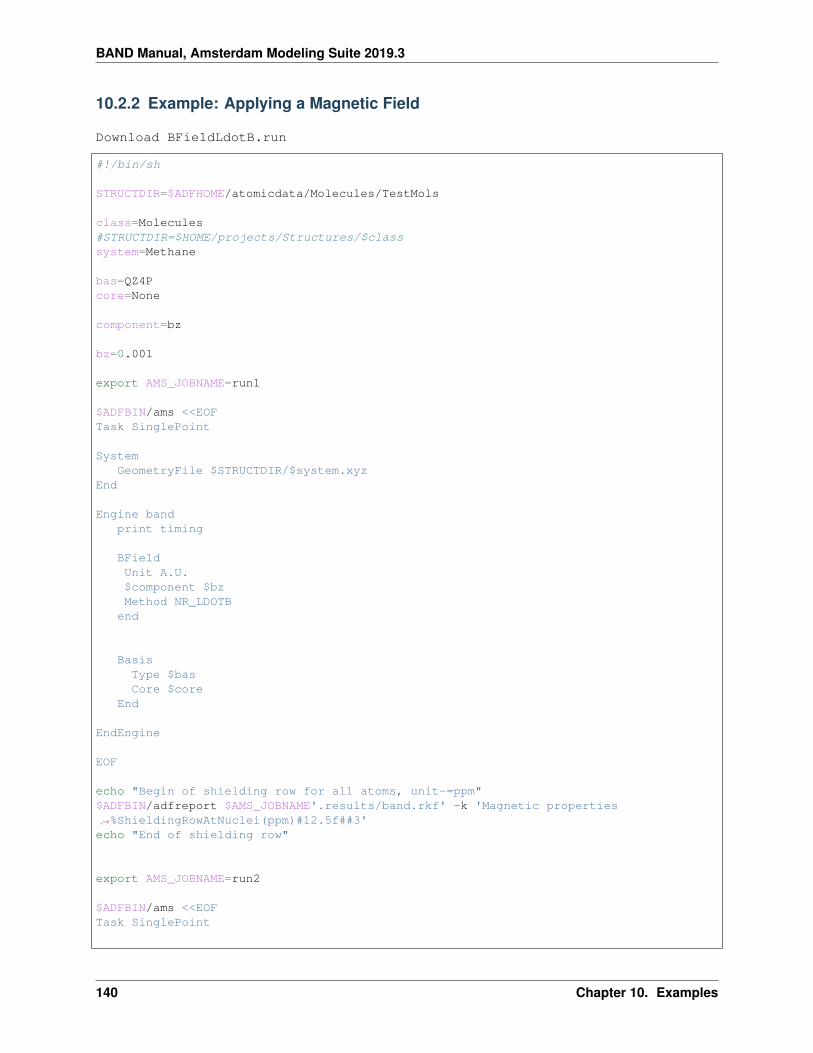
BAND Manual, Amsterdam Modeling Suite 2019.3
10.2.2 Example: Applying a Magnetic Field
Download BFieldLdotB.run
#!/bin/sh
STRUCTDIR=$ADFHOME/atomicdata/Molecules/TestMols
class=Molecules#STRUCTDIR=$HOME/projects/Structures/$classsystem=Methane
bas=QZ4Pcore=None
component=bz
bz=0.001
export AMS_JOBNAME=run1
$ADFBIN/ams <<EOFTask SinglePoint
SystemGeometryFile $STRUCTDIR/$system.xyz
End
Engine bandprint timing
BFieldUnit A.U.$component $bzMethod NR_LDOTB
end
BasisType $basCore $core
End
EndEngine
EOF
echo "Begin of shielding row for all atoms, unit-=ppm"$ADFBIN/adfreport $AMS_JOBNAME'.results/band.rkf' -k 'Magnetic properties→˓%ShieldingRowAtNuclei(ppm)#12.5f##3'echo "End of shielding row"
export AMS_JOBNAME=run2
$ADFBIN/ams <<EOFTask SinglePoint
140 Chapter 10. Examples

BAND Manual, Amsterdam Modeling Suite 2019.3
SystemGeometryFile $STRUCTDIR/$system.xyz
End
Engine bandprint timing
BFieldUnit A.U.$component $bzMethod NR_LDOTBDipole trueDipoleAtom 1
end
BasisType $basCore $core
End
EndEngine
EOF
echo "Begin of shielding row for all atoms, unit-=ppm"$ADFBIN/adfreport $AMS_JOBNAME'.results/band.rkf' -k 'Magnetic properties→˓%ShieldingRowAtNuclei(ppm)#12.5f##3'echo "End of shielding row"
10.2.3 Example: Graphene sheet with dispersion correction
Download Graphene_Dispersion.run
#! /bin/sh
# A normal GGA would give only negligible interaction between two graphene# sheets.
# Use the dispersion option in the XC key block.
# In the first run we use BP86-D, in the second BLYP-D3 and in the third run# BLYP-D3(BJ).
# == First run: dispersion default ==
AMS_JOBNAME=default $ADFBIN/ams <<eor
Task SinglePoint
SystemGeometryFile $ADFHOME/examples/band/Graphene_Dispersion/Graphene_double_layer.xyz
End
Engine Band
10.2. Model Hamiltonians 141

BAND Manual, Amsterdam Modeling Suite 2019.3
XCgga scf bp86dispersion default
End
NumericalQuality Basic
BasisType TZPCore Large
EndEndEngineeor
# == Second run: dispersion Grimme3 ==
AMS_JOBNAME=grimme3 $ADFBIN/ams <<eor
Task SinglePoint
SystemGeometryFile $ADFHOME/examples/band/Graphene_Dispersion/Graphene_double_layer.xyz
End
PropertiesGradients True
End
Engine BandXC
gga scf blypdispersion Grimme3
end
NumericalQuality Basic
BasisType TZPCore Large
EndEndEngineeor
# == Third run: dispersion Grimme3 bjdamp ==
AMS_JOBNAME=grimme3_bjdamp $ADFBIN/ams <<eor
Task SinglePoint
SystemGeometryFile $ADFHOME/examples/band/Graphene_Dispersion/Graphene_double_layer.xyz
End
PropertiesGradients True
End
Engine Band
142 Chapter 10. Examples

BAND Manual, Amsterdam Modeling Suite 2019.3
XCgga scf blypdispersion Grimme3 bjdamp
end
NumericalQuality Basic
BasisType TZPCore Large
EndEndEngineeor
10.2.4 Example: H on perovskite with the COSMO solvation model
Download HonPerovskite_Solvation.run
#! /bin/sh
# We want to model H adsorption on a Perovskite surface in a solution, modeled# by a COSMO surface.
# We create only the COSMO surface above the slab with the# RemovePointsWithNegativeZ option.
$ADFBIN/ams <<eor
Task SinglePoint
SystemAtoms
H 0.0 0.000000000 0.900000000Ca 0.0 0.000000000 0.000000000Ca 0.0 3.535533906 -3.535533906Ti -2.5 -3.535533906 0.000000000Ti -2.5 0.000000000 -3.535533906O 0.0 -3.535533906 0.000000000O 2.5 1.767766953 -1.767766953O 2.5 -1.767766953 -1.767766953
EndLattice
5.0 0.000000000 0.00.0 7.071067812 0.0
EndEnd
PropertiesGradients True
End
Engine BandTITLE Hydrogen on Perovksite wit solvation
SolvationEnabled True
10.2. Model Hamiltonians 143

BAND Manual, Amsterdam Modeling Suite 2019.3
Surf Delleycharge method=inverSolvent
Eps 78.4Rad 1.4
EndEnd
PeriodicSolvationnstar 3SymmetrizeSurfacePoints trueRemovePointsWithNegativeZ true
End
Screeningrmadel 30 ! to speed up the calculation
End
ConvergenceCriterion 1.0e-4
End
BasisType SZCore Large
EndEndEngineeor
10.2.5 Example: Applying a homogeneous electric field
Download EField.run
#!/bin/sh
# With the EFIELD keyword you can specify a static electric field in the# z-direction.
# == first run: field specified in a.u. ==
$ADFBIN/ams <<eor
Task SinglePoint
Systemlattice [Bohr]
15.0 0.0 0.00.0 15.0 0.0
EndAtoms [Bohr]
H 0.0 0.0 0.0Li 0.0 1.0 3.0
EndEnd
Properties
144 Chapter 10. Examples
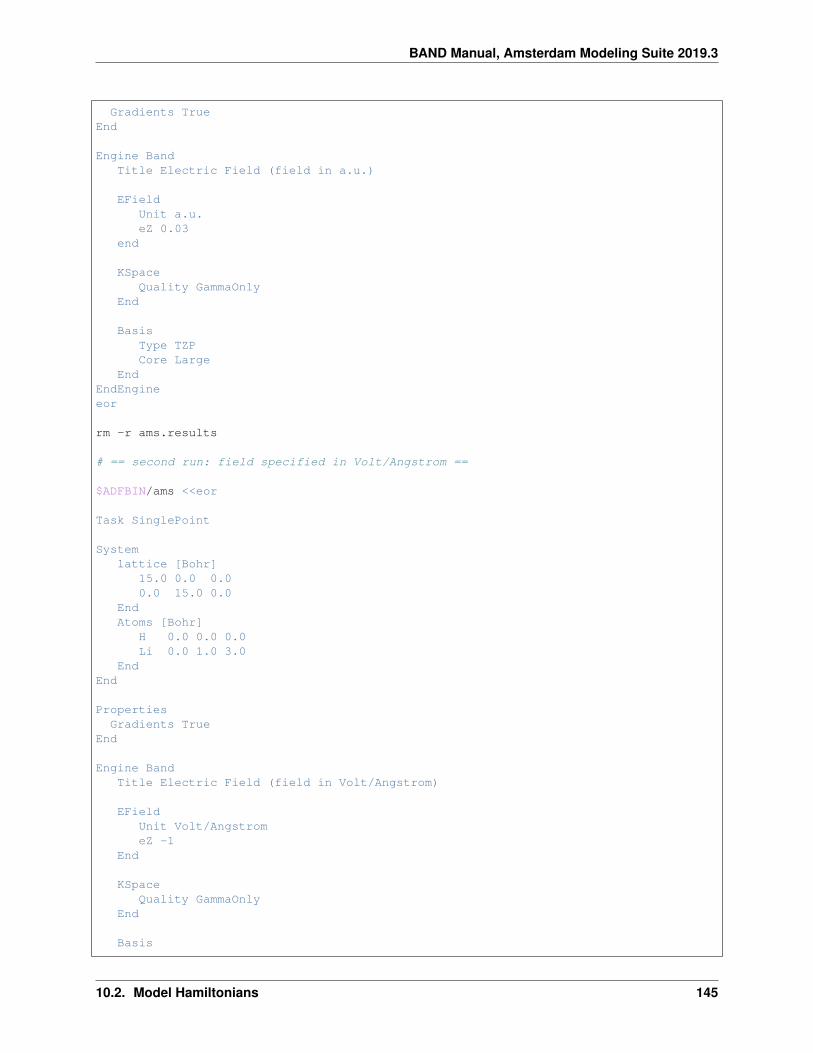
BAND Manual, Amsterdam Modeling Suite 2019.3
Gradients TrueEnd
Engine BandTitle Electric Field (field in a.u.)
EFieldUnit a.u.eZ 0.03
end
KSpaceQuality GammaOnly
End
BasisType TZPCore Large
EndEndEngineeor
rm -r ams.results
# == second run: field specified in Volt/Angstrom ==
$ADFBIN/ams <<eor
Task SinglePoint
Systemlattice [Bohr]
15.0 0.0 0.00.0 15.0 0.0
EndAtoms [Bohr]
H 0.0 0.0 0.0Li 0.0 1.0 3.0
EndEnd
PropertiesGradients True
End
Engine BandTitle Electric Field (field in Volt/Angstrom)
EFieldUnit Volt/AngstromeZ -1
End
KSpaceQuality GammaOnly
End
Basis
10.2. Model Hamiltonians 145

BAND Manual, Amsterdam Modeling Suite 2019.3
Type TZPCore Large
EndEndEngine
eor
10.2.6 Example: Finite nucleus
Download FiniteNucleus.run
#! /bin/sh
# Normally the nucleus is approximated as a point charge. However we can change# this to a finite size. Properties that might be affected are EFG, and the# A-tensor. For such calculations one needs to crank up the precision and also# use a relativistic Hamiltonian.
# == First run: NuclarModel PointCharge ==
AMS_JOBNAME=PointCharge $ADFBIN/ams <<eor
Task SinglePoint
Systemlattice
30.0 0.0 0.0End
AtomsAu 0.000000 0.000000 0.000000
EndEnd
Engine BandNuclearModel PointCharge
EfgEnabled True
End
AtensorEnabled True
End
UnrestrictedRelativityLevel Scalar
End
PropertiesAtNucleirhorho(deformation/scf)vxc[rho(fit)]rho(fit)v(coulomb)
146 Chapter 10. Examples
BAND Manual, Amsterdam Modeling Suite 2019.3
End
RadialDefaultsnr 10000
End
NumericalQuality Good
BasisType TZ2PCore None
End
XCgga PBE
ENDEndEngineeor
# == Second run: NuclearModel Gaussian ==
AMS_JOBNAME=Gaussian $ADFBIN/ams <<eor
Task SinglePoint
Systemlattice
30.0 0.0 0.0End
AtomsAu 0.000000 0.000000 0.000000
EndEnd
Engine BandNuclearModel Gaussian
EfgEnabled True
End
AtensorEnabled True
End
UnrestrictedRelativityLevel Scalar
End
PropertiesAtNucleirhorho(deformation/scf)vxc[rho(fit)]rho(fit)v(coulomb)
End
10.2. Model Hamiltonians 147

BAND Manual, Amsterdam Modeling Suite 2019.3
RadialDefaultsnr 10000
End
NumericalQuality Good
BasisType TZ2PCore None
End
XCgga PBE
ENDEndEngine
eor
10.2.7 Example: Fixing the Band gap of NiO with GGA+U
Download NiO_Hubbard.run
#! /bin/sh
# With the UNRESTRICTED keyword we do a spin polarized calculation.
# With the HubbardU key block we set up the GGA+U calculation. You need to# specify per atom type (only two here, Ni, and O) the U and the l-value to# which it should be applied.
$ADFBIN/ams <<eor
Task SinglePoint
SystemAtoms
Ni 0.0 0.0 0.0O 2.085 2.085 2.085
End
Lattice0.000 2.085 2.0852.085 0.000 2.0852.085 2.085 0.000
EndEnd
Engine BandTitle NiO GGA+U (Hubbard)
Unrestricted
HubbardUEnabled True
148 Chapter 10. Examples
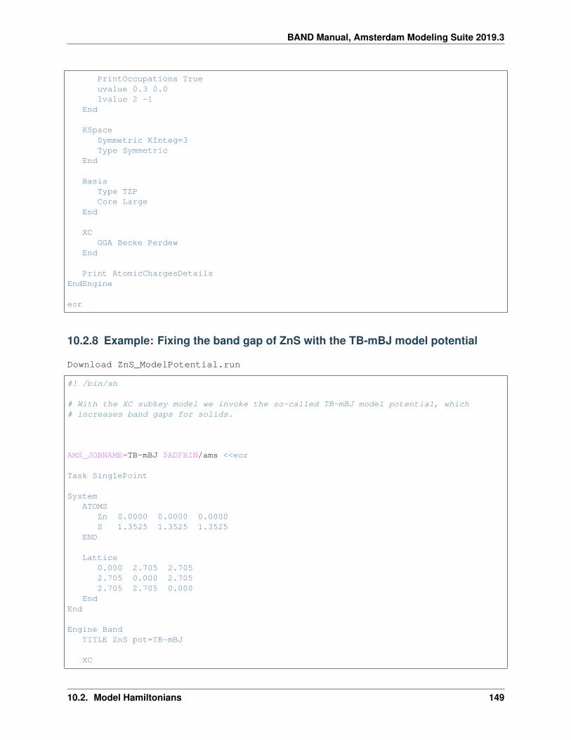
BAND Manual, Amsterdam Modeling Suite 2019.3
PrintOccupations Trueuvalue 0.3 0.0lvalue 2 -1
End
KSpaceSymmetric KInteg=3Type Symmetric
End
BasisType TZPCore Large
End
XCGGA Becke Perdew
End
Print AtomicChargesDetailsEndEngine
eor
10.2.8 Example: Fixing the band gap of ZnS with the TB-mBJ model potential
Download ZnS_ModelPotential.run
#! /bin/sh
# With the XC subkey model we invoke the so-called TB-mBJ model potential, which# increases band gaps for solids.
AMS_JOBNAME=TB-mBJ $ADFBIN/ams <<eor
Task SinglePoint
SystemATOMS
Zn 0.0000 0.0000 0.0000S 1.3525 1.3525 1.3525
END
Lattice0.000 2.705 2.7052.705 0.000 2.7052.705 2.705 0.000
EndEnd
Engine BandTITLE ZnS pot=TB-mBJ
XC
10.2. Model Hamiltonians 149

BAND Manual, Amsterdam Modeling Suite 2019.3
model TB-mBJEND
BasisType DZCore Large
EndEndEngineeor
AMS_JOBNAME=GLLB-SC $ADFBIN/ams <<eor
Task SinglePoint
SystemATOMS
Zn 0.0000 0.0000 0.0000S 1.3525 1.3525 1.3525
ENDLattice
0.000 2.705 2.7052.705 0.000 2.7052.705 2.705 0.000
EndEnd
Engine BandTITLE ZnS pot=GLLB-SC
XCmodel GLLB-SC
END
BasisType DZCore Large
EndEndEngineeor
AMS_JOBNAME=lb94 $ADFBIN/ams <<eor
Task SinglePoint
SystemAtomsH 0.000000000 0.000000000 -0.370500000H 0.000000000 0.000000000 0.370500000End
End
Engine BandTitle H2 pot=lb94
XCmodel lb94
150 Chapter 10. Examples

BAND Manual, Amsterdam Modeling Suite 2019.3
end
BasisType TZPCore Large
EndEndEngineeor
10.2.9 Example: DFT-1/2 method for Silicon
Download DFTHalf_Si.run
#! /bin/sh
"$ADFBIN/ams" <<eor
Task SinglePointSystem
AtomsSi -0.67875 -0.67875 -0.67875Si 0.67875 0.67875 0.67875
EndLattice
0.0 2.715 2.7152.715 0.0 2.7152.715 2.715 0.0
EndEnd
Engine BAND
# To get better results one should use a larger basis set and# a better k-space quality (e.g. 'Basis Type=TZ2P' and 'KSpace Quality=Good')
Basis Type=DZP
XCLDA SCF VWNDFTHalf
Enabled YesActiveAtomtype
AtomType SiIonicCharge 0.1ScreeningCutOffs 2.0 4.0 6.0
EndEnd
EndEndEngineeor
10.2. Model Hamiltonians 151
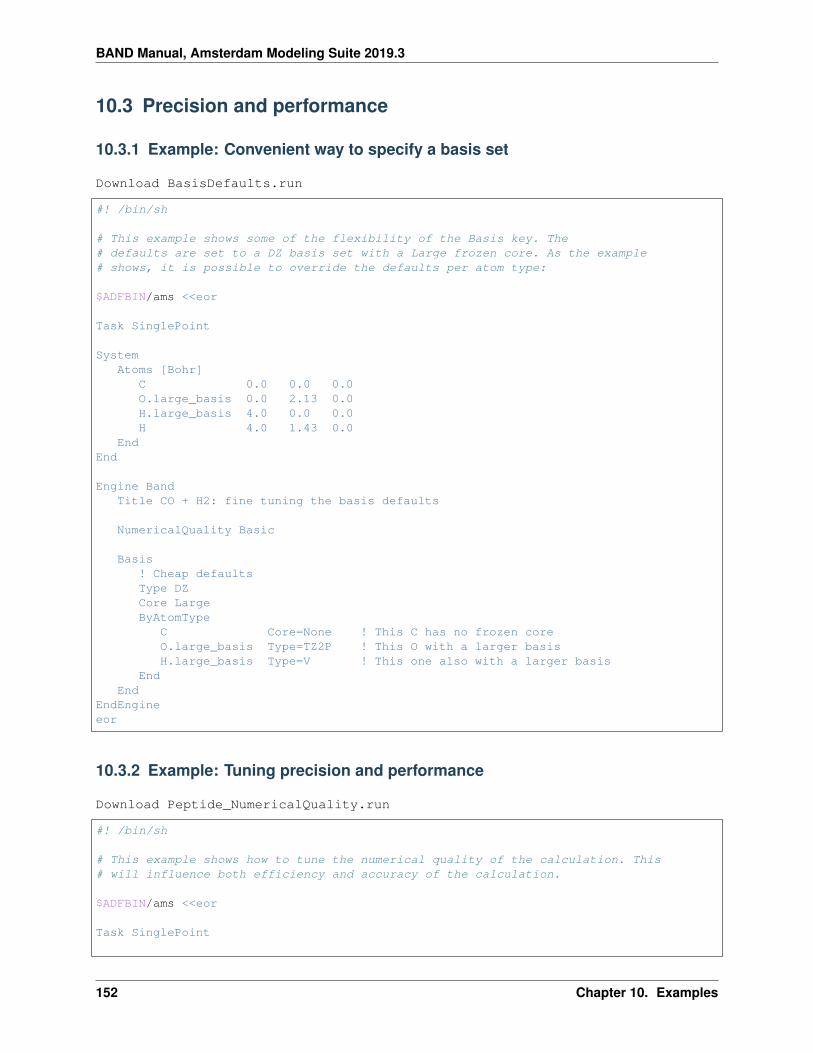
BAND Manual, Amsterdam Modeling Suite 2019.3
10.3 Precision and performance
10.3.1 Example: Convenient way to specify a basis set
Download BasisDefaults.run
#! /bin/sh
# This example shows some of the flexibility of the Basis key. The# defaults are set to a DZ basis set with a Large frozen core. As the example# shows, it is possible to override the defaults per atom type:
$ADFBIN/ams <<eor
Task SinglePoint
SystemAtoms [Bohr]
C 0.0 0.0 0.0O.large_basis 0.0 2.13 0.0H.large_basis 4.0 0.0 0.0H 4.0 1.43 0.0
EndEnd
Engine BandTitle CO + H2: fine tuning the basis defaults
NumericalQuality Basic
Basis! Cheap defaultsType DZCore LargeByAtomType
C Core=None ! This C has no frozen coreO.large_basis Type=TZ2P ! This O with a larger basisH.large_basis Type=V ! This one also with a larger basis
EndEnd
EndEngineeor
10.3.2 Example: Tuning precision and performance
Download Peptide_NumericalQuality.run
#! /bin/sh
# This example shows how to tune the numerical quality of the calculation. This# will influence both efficiency and accuracy of the calculation.
$ADFBIN/ams <<eor
Task SinglePoint
152 Chapter 10. Examples

BAND Manual, Amsterdam Modeling Suite 2019.3
SystemATOMS
C -2.543276676 0.646016253 -0.226282061C -1.380007216 -0.349821933 -0.099968062C 1.066549862 -0.581911934 -0.064823014C 2.223931363 0.423839954 -0.118070453N -0.149937993 0.193000383 -0.179010633N 3.452833267 -0.128914507 -0.101813389O -1.589886979 -1.564606357 0.062390357O 2.010772661 1.647347397 -0.186192833H -2.480330907 1.422845016 0.554868474H 3.629655835 -1.142731500 -0.018098016H -2.511564496 1.180719545 -1.193540463H 0.024515371 1.206808884 -0.244500253H 1.160598100 -1.320381370 -0.884522980H 1.071343640 -1.136930542 0.888913220
ENDLattice
7.211585775 0.000000000 0.000000000End
End
Engine BandTITLE Quality
NumericalQuality Normal
ZlmFitQuality Normal
End
BeckeGridQuality Basic
End
KSpaceQuality Basic
End
SoftConfinementQuality VeryGood
End
BasisType DZCore Large
End
XCGGA PBE
ENDEndEngineeor
10.3. Precision and performance 153

BAND Manual, Amsterdam Modeling Suite 2019.3
10.3.3 Example: Multiresolution
Download Multiresolution_H2O.run
#! /bin/sh
# This example demonstrates how to use different levels of numerical precision# for different regions, with the aim of increasing computational efficiency.
# Let us assume that we are interested in having an accurate description only# for a subregion of a large chemical system (in this simple example, the# central water molecule). The system can be divided into sub-regions and# different levels of numerical accuracy can be used for each of these sub-# regions.
# In this example we will tweak:# - the basis set (Basis)# - the numerical integration (BeckeGrid)# - the density fitting for Coulomb potential (ZlmFit)# - the fit-set used in the Hartree-Fock Resolution of identity (RIHartreeFock)
# Note: For the atoms that have not been explicitly defined in the# AtomDepQuality sub-blocks, the quality defined in NumericalQuality will be# used (Normal, in this example).
$ADFBIN/ams <<eor
Task SinglePoint
SystemAtoms
O.Accurate 0.00000000 0.00000000 0.00000000 ! 1H.Accurate 0.40399229 -0.65578342 0.63241539 ! 2H.Accurate 0.81410032 0.55624569 -0.23129097 ! 3O.Near -3.02535626 -0.08473104 -0.47678489 ! 4H.Near -2.56531481 0.62644005 0.07759386 ! 5H.Near -2.25289644 -0.61700366 -0.80790649 ! 6O.Near 2.95394790 -0.54939973 -0.38206034 ! 7H.Near 3.91427727 -0.21304908 -0.44738291 ! 8H.Near 2.87780992 -1.13241278 -1.20853726 ! 9O.Far -5.95425742 -0.56764616 -0.02016682 ! 10H.Far -5.26308282 -0.46969096 0.69255963 ! 11H.Far -5.42117992 -0.54361203 -0.86443121 ! 12O.Far 6.25171470 -0.62004899 -0.03702467 ! 13H.Far 6.16508647 -1.38696453 0.58541903 ! 14H.Far 7.09161199 -0.16700550 0.23679419 ! 15
EndEnd
Engine BandXC
LibXC B3LYPEnd
! =============================================================! Set the NumerialQuality to be used for the atoms that are not! explicitely defined in AtomDepQuality! =============================================================
154 Chapter 10. Examples
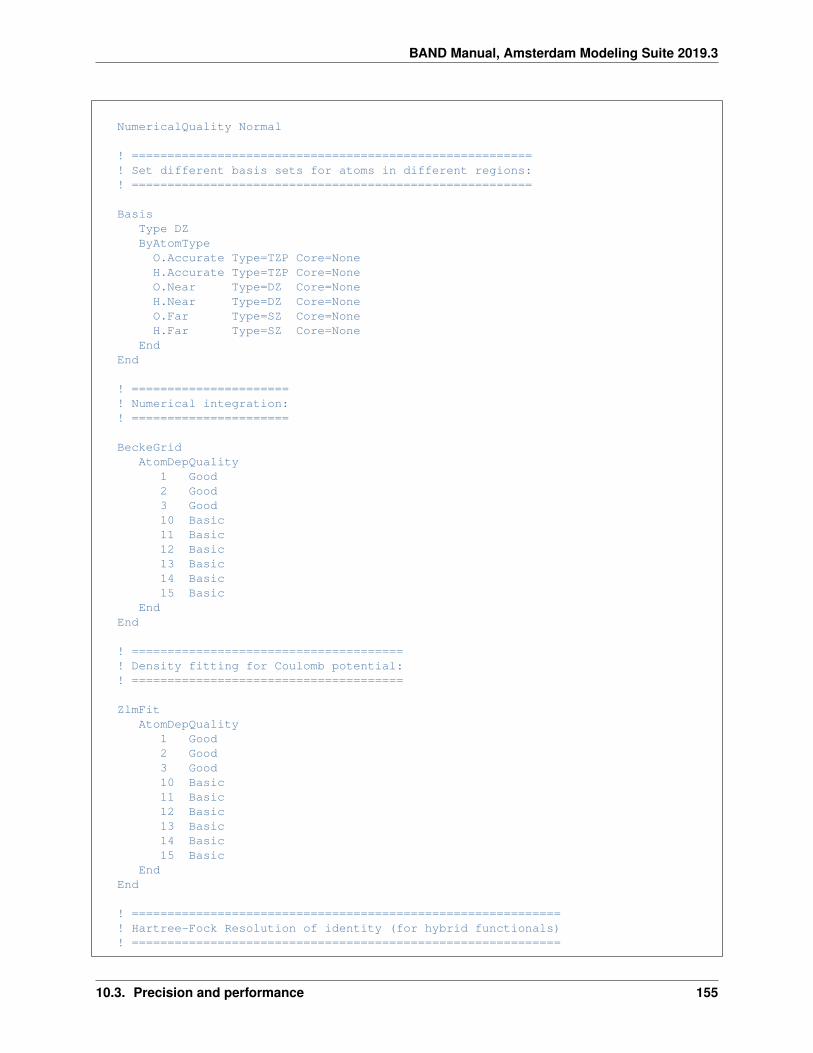
BAND Manual, Amsterdam Modeling Suite 2019.3
NumericalQuality Normal
! ========================================================! Set different basis sets for atoms in different regions:! ========================================================
BasisType DZByAtomType
O.Accurate Type=TZP Core=NoneH.Accurate Type=TZP Core=NoneO.Near Type=DZ Core=NoneH.Near Type=DZ Core=NoneO.Far Type=SZ Core=NoneH.Far Type=SZ Core=None
EndEnd
! ======================! Numerical integration:! ======================
BeckeGridAtomDepQuality
1 Good2 Good3 Good10 Basic11 Basic12 Basic13 Basic14 Basic15 Basic
EndEnd
! ======================================! Density fitting for Coulomb potential:! ======================================
ZlmFitAtomDepQuality
1 Good2 Good3 Good10 Basic11 Basic12 Basic13 Basic14 Basic15 Basic
EndEnd
! ============================================================! Hartree-Fock Resolution of identity (for hybrid functionals)! ============================================================
10.3. Precision and performance 155

BAND Manual, Amsterdam Modeling Suite 2019.3
RIHartreeFockAtomDepQuality
1 Good2 Good3 Good10 Basic11 Basic12 Basic13 Basic14 Basic15 Basic
EndEnd
EndEngine
eor
10.3.4 Example: BSSE correction
Download BSSE.run
#!/bin/bash
# This example shows how to calculate the basis set superposition error for the# interaction of CO with H2. In this shell script we loop over progressively# better basis sets.
for bas in DZ TZ2P QZ4Pdo
core=Large
$ADFBIN/ams <<eorTask SinglePointSystem
Atoms [Bohr]C 0 0 0O 2.13 0 0H 0 0 6H 1.5 0 6
EndEnd
Engine BandBasisType $basCore $core
EndEndEngineeor
ECOH2=`$ADFBIN/adfreport ams.results/band.rkf -r 'Bond energies%final bond energy'`rm -r ams.results
$ADFBIN/ams <<eor
156 Chapter 10. Examples
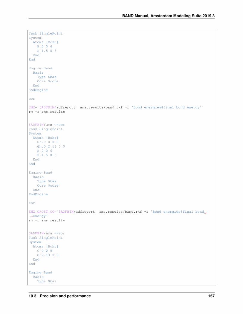
BAND Manual, Amsterdam Modeling Suite 2019.3
Task SinglePointSystem
Atoms [Bohr]H 0 0 6H 1.5 0 6
EndEnd
Engine BandBasisType $basCore $core
EndEndEngine
eor
EH2=`$ADFBIN/adfreport ams.results/band.rkf -r 'Bond energies%final bond energy'`rm -r ams.results
$ADFBIN/ams <<eorTask SinglePointSystem
Atoms [Bohr]Gh.C 0 0 0Gh.O 2.13 0 0H 0 0 6H 1.5 0 6
EndEnd
Engine BandBasisType $basCore $core
EndEndEngine
eor
EH2_GHOST_CO=`$ADFBIN/adfreport ams.results/band.rkf -r 'Bond energies%final bond→˓energy'`rm -r ams.results
$ADFBIN/ams <<eorTask SinglePointSystem
Atoms [Bohr]C 0 0 0O 2.13 0 0
EndEnd
Engine BandBasisType $bas
10.3. Precision and performance 157

BAND Manual, Amsterdam Modeling Suite 2019.3
Core $coreEnd
EndEngine
eor
ECO=`$ADFBIN/adfreport ams.results/band.rkf -r 'Bond energies%final bond energy'`rm -r ams.results
$ADFBIN/ams <<eorTask SinglePointSystem
Atoms [Bohr]C 0 0 0O 2.13 0 0Gh.H 0 0 6Gh.H 1.5 0 6
EndEnd
Engine BandBasisType $basCore $core
EndEndEngine
eor
ECO_GHOST_H2=`$ADFBIN/adfreport ams.results/band.rkf -r 'Bond energies%final bond→˓energy'`rm -r ams.results
EV=27.212echo "Start report"echo "basis set: $bas"echo "H2 + CO : $ECOH2"echo "H2 : $EH2"echo "H2 (with ghost CO) : $EH2_GHOST_CO"echo "CO : $ECO"echo "CO (with ghost H2) : $ECO_GHOST_H2"BSSEEV=`$ADFBIN/startpython -c "print (( $EH2 - $EH2_GHOST_CO + $ECO - $ECO_GHOST_H2→˓) *$EV)"`echo "BSSE correction: $BSSEEV (eV)"BOND1EV=`$ADFBIN/startpython -c "print (( $ECOH2 - $EH2 - $ECO ) *$EV)"`BOND2EV=`$ADFBIN/startpython -c "print ($BOND1EV + $BSSEEV)"`echo "Bond energy: $BOND1EV (eV)"echo "Bond energy + BSSE: $BOND2EV (eV)"echo "End report"
done
158 Chapter 10. Examples
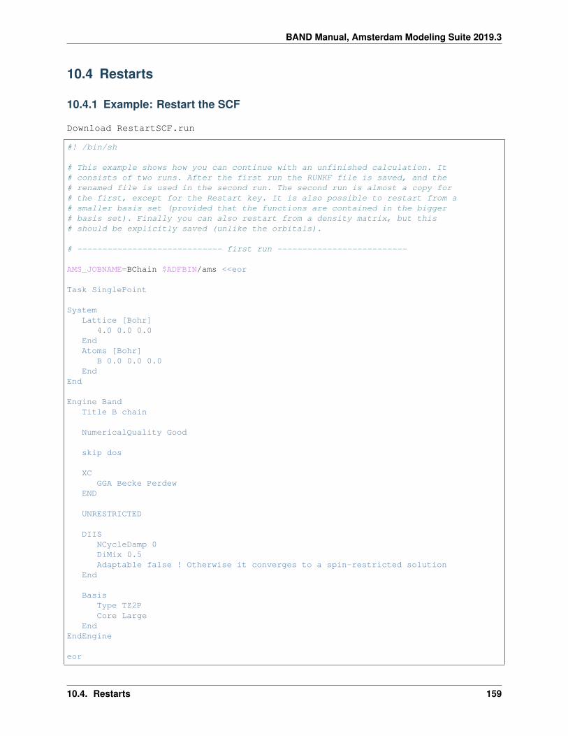
BAND Manual, Amsterdam Modeling Suite 2019.3
10.4 Restarts
10.4.1 Example: Restart the SCF
Download RestartSCF.run
#! /bin/sh
# This example shows how you can continue with an unfinished calculation. It# consists of two runs. After the first run the RUNKF file is saved, and the# renamed file is used in the second run. The second run is almost a copy for# the first, except for the Restart key. It is also possible to restart from a# smaller basis set (provided that the functions are contained in the bigger# basis set). Finally you can also restart from a density matrix, but this# should be explicitly saved (unlike the orbitals).
# ----------------------------- first run --------------------------
AMS_JOBNAME=BChain $ADFBIN/ams <<eor
Task SinglePoint
SystemLattice [Bohr]
4.0 0.0 0.0EndAtoms [Bohr]
B 0.0 0.0 0.0End
End
Engine BandTitle B chain
NumericalQuality Good
skip dos
XCGGA Becke Perdew
END
UNRESTRICTED
DIISNCycleDamp 0DiMix 0.5Adaptable false ! Otherwise it converges to a spin-restricted solution
End
BasisType TZ2PCore Large
EndEndEngine
eor
10.4. Restarts 159

BAND Manual, Amsterdam Modeling Suite 2019.3
# ----------------------------- second run --------------------------
AMS_JOBNAME=restart_1 $ADFBIN/ams <<eor
Task SinglePoint
SystemLattice [Bohr]
4.0 0.0 0.0EndAtoms [Bohr]
B 0.0 0.0 0.0End
End
Engine BandTitle B chain restart
NumericalQuality Good
XCGGA Becke Perdew
END
UNRESTRICTED
RestartFile BChain.results/band.rkfscf
end
BasisType TZ2PCore Large
EndEndEngine
eor
# ----------------------------- third run --------------------------
AMS_JOBNAME=BChain_SZ $ADFBIN/ams <<eor
Task SinglePoint
SystemLattice [Bohr]
4.0 0.0 0.0EndAtoms [Bohr]
B 0.0 0.0 0.0End
End
Engine BandTitle B chain bas_SZ
160 Chapter 10. Examples

BAND Manual, Amsterdam Modeling Suite 2019.3
NumericalQuality Good
Save DensityMatrix
skip dos
XCGGA Becke Perdew
END
UNRESTRICTED
DIISNCycleDamp 0DiMix 0.3Adaptable false ! Otherwise it converges to a spin-restricted solution
End
BasisType SZCore Large
EndEndEngine
eor
# ----------------------------- fourth run --------------------------
AMS_JOBNAME=restart_2 $ADFBIN/ams <<eor
Task SinglePoint
SystemLattice [Bohr]
4.0 0.0 0.0EndAtoms [Bohr]
B 0.0 0.0 0.0End
End
Engine BandTitle B chain restart bas_SZ from density matrix
NumericalQuality Good
XCGGA Becke Perdew
END
UNRESTRICTED
RestartFile BChain_SZ.results/band.rkfscfuseDensityMatrix true
end
10.4. Restarts 161
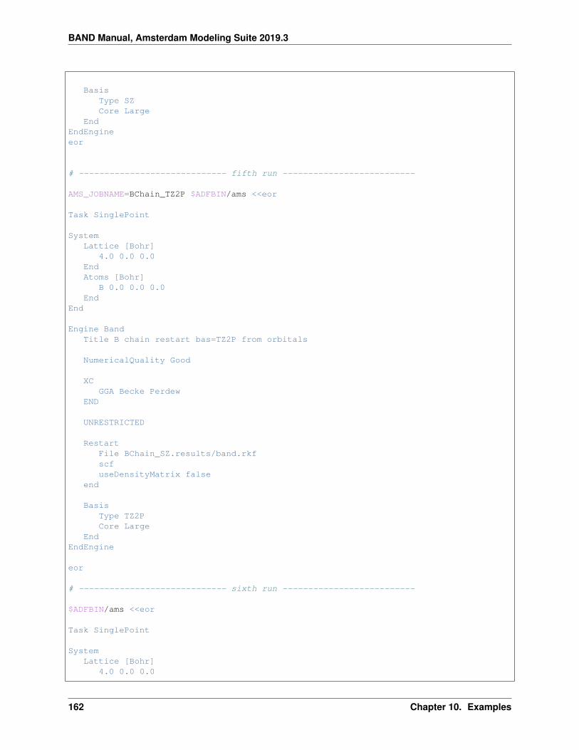
BAND Manual, Amsterdam Modeling Suite 2019.3
BasisType SZCore Large
EndEndEngineeor
# ----------------------------- fifth run --------------------------
AMS_JOBNAME=BChain_TZ2P $ADFBIN/ams <<eor
Task SinglePoint
SystemLattice [Bohr]
4.0 0.0 0.0EndAtoms [Bohr]
B 0.0 0.0 0.0End
End
Engine BandTitle B chain restart bas=TZ2P from orbitals
NumericalQuality Good
XCGGA Becke Perdew
END
UNRESTRICTED
RestartFile BChain_SZ.results/band.rkfscfuseDensityMatrix false
end
BasisType TZ2PCore Large
EndEndEngine
eor
# ----------------------------- sixth run --------------------------
$ADFBIN/ams <<eor
Task SinglePoint
SystemLattice [Bohr]
4.0 0.0 0.0
162 Chapter 10. Examples

BAND Manual, Amsterdam Modeling Suite 2019.3
EndAtoms [Bohr]
B 0.0 0.0 0.0End
End
Engine BandTitle B chain restart bas=TZ2P from density matrix (bas_SZ)
NumericalQuality Good
XCGGA Becke Perdew
END
UNRESTRICTED
RestartFile BChain_SZ.results/band.rkfscfuseDensityMatrix true
end
BasisType TZ2PCore Large
EndEndEngineeor
10.4.2 Example: Restart SCF for properties calculation
Download RestartProperties.run
#!/bin/sh
# This example shows how to restart the SCF and compute various properties, like# a density of states, and a band structure plot, or the effective mass.
# =======================# polyethylene .xyz file:# =======================
cat <<eor > polyethylene.xyz6
C -0.623348981 -0.055000000 0.425969423C 0.633348981 0.015000000 -0.422636089H -0.633348981 0.964974570 1.055290696H -0.623348981 -0.914974570 1.055290696H 0.633348981 0.904974570 -1.051957363H 0.613348981 -0.914974570 -1.061957363VEC1 2.553395923 0.000000000 0.000000000eor
# ===============================================
10.4. Restarts 163

BAND Manual, Amsterdam Modeling Suite 2019.3
# Simple single point calculation (no properties)# ===============================================
AMS_JOBNAME=ToBeRestarted $ADFBIN/ams <<eor
Task SinglePoint
SystemGeometryFile polyethylene.xyz
End
Engine BandUnrestricted True
EndEngineeor
# ===================================# Restart and compute some properties# ===================================
AMS_JOBNAME=prop $ADFBIN/ams <<eor
Task SinglePoint
SystemGeometryFile polyethylene.xyz
End
Engine BandUnrestricted True
RestartSCFFile ToBeRestarted.results/band.rkf
End
DOSEnabled True
End
BandStructureEnabled TrueDeltaK 0.3EnergyAboveFermi 10.0
End
EffectiveMassEnabled True
EndEndEngineeor
echo 'Extract some properties from the rkf file:'
echo "Density of States:"$ADFBIN/adfreport prop.results/band.rkf -r 'DOS%Total DOS##1'
164 Chapter 10. Examples
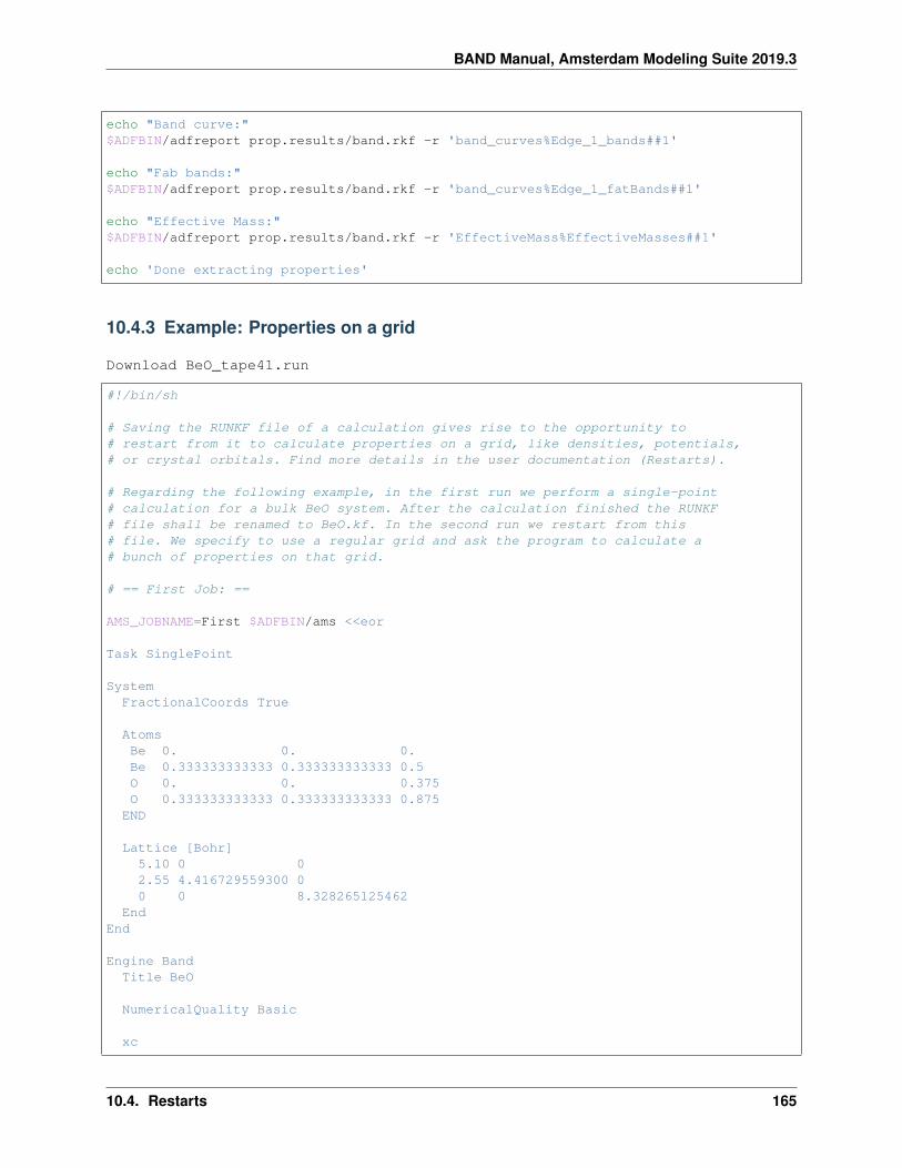
BAND Manual, Amsterdam Modeling Suite 2019.3
echo "Band curve:"$ADFBIN/adfreport prop.results/band.rkf -r 'band_curves%Edge_1_bands##1'
echo "Fab bands:"$ADFBIN/adfreport prop.results/band.rkf -r 'band_curves%Edge_1_fatBands##1'
echo "Effective Mass:"$ADFBIN/adfreport prop.results/band.rkf -r 'EffectiveMass%EffectiveMasses##1'
echo 'Done extracting properties'
10.4.3 Example: Properties on a grid
Download BeO_tape41.run
#!/bin/sh
# Saving the RUNKF file of a calculation gives rise to the opportunity to# restart from it to calculate properties on a grid, like densities, potentials,# or crystal orbitals. Find more details in the user documentation (Restarts).
# Regarding the following example, in the first run we perform a single-point# calculation for a bulk BeO system. After the calculation finished the RUNKF# file shall be renamed to BeO.kf. In the second run we restart from this# file. We specify to use a regular grid and ask the program to calculate a# bunch of properties on that grid.
# == First Job: ==
AMS_JOBNAME=First $ADFBIN/ams <<eor
Task SinglePoint
SystemFractionalCoords True
AtomsBe 0. 0. 0.Be 0.333333333333 0.333333333333 0.5O 0. 0. 0.375O 0.333333333333 0.333333333333 0.875END
Lattice [Bohr]5.10 0 02.55 4.416729559300 00 0 8.328265125462
EndEnd
Engine BandTitle BeO
NumericalQuality Basic
xc
10.4. Restarts 165

BAND Manual, Amsterdam Modeling Suite 2019.3
GGA BP86end
BasisType DZCore large
endEndEngineeor
# == Second Job: ==
AMS_JOBNAME=Second $ADFBIN/ams <<eor
Task SinglePoint
SystemFractionalCoords True
AtomsBe 0. 0. 0.Be 0.333333333333 0.333333333333 0.5O 0. 0. 0.375O 0.333333333333 0.333333333333 0.875END
Lattice [Bohr]5.10 0 02.55 4.416729559300 00 0 8.328265125462
EndEnd
Engine BandTitle BeO_restart
RestartFile First.results/band.rkfDensityPlot
End
GridType Coarse
End
DensityPlotrho(deformation/fit) ! FITDENSITY_deformation_scfrho(fit) ! FITDENSITY_total_scfrho(atoms) ! ATOMIC_densityv(coulomb/atoms) ! ATOMIC_coulombPotv(coulomb) ! COULOMBPOTENTIAL_scfvxc[rho(fit)] ! XCPOTENTIAL_scf
End
NumericalQuality Basic
xcGGA BP86
166 Chapter 10. Examples

BAND Manual, Amsterdam Modeling Suite 2019.3
end
BasisType DZCore large
endEndEngineeor
NSCM=1export NSCMecho ""echo "Begin TOC of tape41"
$ADFBIN/dmpkf -n 1 Second.results/TAPE41 --toc
echo "End TOC of tape41"
10.5 NEGF
10.5.1 Example: Main NEGF flavors
Download NEGF_Cr_wire.run
#! /bin/sh
# This example shows how to use the NEGF functionality.# Note: Setting up a NEGF calculation is quite hard without the GUI.
# It starts of with Method 1: the non-self consistent approach. Here, BAND# merely serves to provide matrix elements, being unaware of the electrodes.
# Then follows Method 2: here the NEGF density is really used to calculate the# matrix elements.
# Method 3 is a variation on Method 2, and includes an extra alignment run.
# ==============================================================================# Method #1: non-self consistent NEGF (uses the conductance program, like DFTB)# ==============================================================================
# ========================= Method #1. Run #1 ==============================
AMS_JOBNAME=lead_1 $ADFBIN/ams <<eor
Task SinglePoint
SystemATOMS
Cr.1 0.0 0.0 0.0Cr.2 2.5 0.0 0.0
END
10.5. NEGF 167

BAND Manual, Amsterdam Modeling Suite 2019.3
Lattice5.0 0.0 0.0
EndEnd
Engine BandTitle method_1_run_1
KSpaceQuality Good
End
NumericalQuality Basic
BasisType DZCore Large
End
Unrestricted
StoreHamiltonian2EndEngineeor
# ======================== Method #1. Run #2 ===============================
AMS_JOBNAME=scattering_1 $ADFBIN/ams <<eor
Task SinglePoint
SystemATOMS
Cr.1L -10.0 0.0 0.0Cr.2L -7.5 0.0 0.0Cr.C -5.0 0.0 0.0Cr.C -2.5 0.0 0.0Cr.C 0.0 0.0 0.0Cr.C 2.5 0.0 0.0Cr.C 5.0 0.0 0.0Cr.1R 7.5 0.0 0.0Cr.2R 10.0 0.0 0.0
END
Lattice22.5 0.0 0.0
EndEnd
Engine BandTitle method_1_run_2
NumericalQuality Basic
BasisType DZCore Large
End
168 Chapter 10. Examples

BAND Manual, Amsterdam Modeling Suite 2019.3
Unrestricted
StoreHamiltonian2StoreHamAsMol
EndEngine
eor
# ========================== Method #1. Run #3 =============================
$ADFBIN/conductance <<EOFEnergyGrid min=-5 max=5 num=200Files
Leads lead_1.results/band.rkfScattering scattering_1.results/band.rkf
End
EOF
# Compy the content of the "reseults" section from ConductanceResults.kf to band.rkf→˓and rename the section to NEGF$ADFBIN/cpkf "ConductanceResults.kf" "scattering_1.results/band.rkf" "results --→˓rename NEGF"
echo "Extract transmisstion from rkf file (Method 1)"$ADFBIN/adfreport scattering_1.results/band.rkf -r "NEGF%transmission#12.5f##1"
# ==============================================================================# Method #2: self consistent NEGF without alignment# ==============================================================================
# ========================= Method #2. Run #1 ==============================
AMS_JOBNAME=lead_2 $ADFBIN/ams <<eor
Task SinglePoint
SystemATOMS
Cr.1 0.0 0.0 0.0Cr.2 2.5 0.0 0.0
END
Lattice5.0 0.0 0.0End
End
Engine BandTitle method_2_run_1
KSpaceQuality Good
End
10.5. NEGF 169

BAND Manual, Amsterdam Modeling Suite 2019.3
NumericalQuality Basic
BasisType DZCore Large
End
UnrestrictedStoreHamiltonian2
EndEngine
eor
# ============================= Method #2. Run #2 ==========================
$ADFBIN/sgf <<eorTITLE Test for NEGF inputsSAVE SIGMASURFACEGF
RKFFileName lead_2.results/band.rkfSCMCodeKT 0.001ContourQuality normal
ENDeor
mv SigmaSCM Sigma.kf
# ============================= Method #2. Run #3 ==========================
AMS_JOBNAME=scattering_2 $ADFBIN/ams <<eor
Task SinglePoint
SystemATOMS
Cr.1L -10.0 0.0 0.0Cr.2L -7.5 0.0 0.0Cr.C -5.0 0.0 0.0Cr.C -2.5 0.0 0.0Cr.C 0.0 0.0 0.0Cr.C 2.5 0.0 0.0Cr.C 5.0 0.0 0.0Cr.1R 7.5 0.0 0.0Cr.2R 10.0 0.0 0.0
ENDEnd
Engine BandTitle method_2_run_3
NumericalQuality Basic
BasisType DZCore Large
End
170 Chapter 10. Examples

BAND Manual, Amsterdam Modeling Suite 2019.3
UnrestrictedNEGFLeadFile lead_2.results/band.rkfSGFFile Sigma.kfApplyShift2 FalseContourQuality normalEMin -5EMax 5NE 200
EndEndEngineeor
echo "Extract transmisstion from rkf file (Method 2)"$ADFBIN/adfreport scattering_2.results/band.rkf -r "NEGF%transmission#12.5f##1"
# ==============================================================================# Method #3: self consistent NEGF wit alignment run# ==============================================================================
# ======================= Method #3. Run #1 ================================
AMS_JOBNAME=lead_3 $ADFBIN/ams <<eor
Task SinglePoint
SystemATOMS
Cr.1 0.0 0.0 0.0Cr.2 2.5 0.0 0.0
ENDLattice5.0 0.0 0.0End
End
Engine BandTitle method_3_run_1
KSpaceQuality Good
End
NumericalQuality Basic
BasisType DZCore Large
End
UnrestrictedStoreHamiltonian2
EndEngineeor
# ============================ Method #3. Run #2 ===========================
10.5. NEGF 171

BAND Manual, Amsterdam Modeling Suite 2019.3
$ADFBIN/sgf <<eorTITLE Test for NEGF inputsSAVE SIGMASURFACEGF
RKFFileName lead_3.results/band.rkfSCMCodeKT 0.001ContourQuality normal
ENDeor
mv SigmaSCM Sigma.kf
# ============================ Method #3. Run #3 ===========================
AMS_JOBNAME=align $ADFBIN/ams <<eor
Task SinglePoint
SystemATOMS
Cr.1L 0.0 0.0 0.0Cr.2L 2.5 0.0 0.0Cr.C 5.0 0.0 0.0Cr.C 7.5 0.0 0.0Cr.C 10.0 0.0 0.0Cr.C 12.5 0.0 0.0Cr.1R 15.0 0.0 0.0Cr.2R 17.5 0.0 0.0
ENDEnd
Engine BandTitle method_3_run_3
NumericalQuality Basic
BasisType DZCore Large
End
UnrestrictedNEGFDoAlignment TrueLeadFile lead_3.results/band.rkfSGFFile Sigma.kfContourQuality normalEMin -5.0EMax 5.0NE 200AlignChargeTol 0.0001
EndEndEngineeor
172 Chapter 10. Examples

BAND Manual, Amsterdam Modeling Suite 2019.3
# ============================= Method #3. Run #4 ===========================
AMS_JOBNAME=scattering_3 $ADFBIN/ams <<eor
Task SinglePoint
SystemATOMS
Cr.1L -10.0 0.0 0.0Cr.2L -7.5 0.0 0.0Cr.C -5.0 0.0 0.0Cr.C -2.5 0.0 0.0Cr.C 0.0 0.0 0.0Cr.C 2.5 0.0 0.0Cr.C 5.0 0.0 0.0Cr.1R 7.5 0.0 0.0Cr.2R 10.0 0.0 0.0
ENDEnd
engine BandTitle method_3_run_4
NumericalQuality Basic
BasisType DZCore Large
End
Unrestricted
NEGFLeadFile lead_3.results/band.rkfSGFFile Sigma.kfAlignmentFile align.results/band.rkfContourQuality normalEMin -5.0EMax 5.0NE 200
EndEndEngineeor
echo "Extract transmisstion from rkf file (Method 2)"$ADFBIN/adfreport scattering_3.results/band.rkf -r "NEGF%transmission#12.5f##1"
10.5.2 Example: NEGF with bias
Download NEGF_bias.run
#! /bin/sh
# This example shows how to use the NEGF key when including a bias potential# between the electrodes. It starts of with the usual tight-binding run,# followed by an SGF one. The alignment run is omitted. Finally, there is a loop
10.5. NEGF 173

BAND Manual, Amsterdam Modeling Suite 2019.3
# over bias potentials. Here the scale feature of the FuzzyPotential is used.# The current is appended to a text file, which one could plot eg. with gnuplot.
# Note: Setting up a NEGF calculation is quite hard without the GUI.
AMS_JOBNAME=tight-binding $ADFBIN/ams <<eor
Task SinglePoint
SystemAtoms
Li.1 0.0 0.0 0.0Li.2 2.876 0.0 0.0Li.3 5.752 0.0 0.0
EndLattice8.628 0.0 0.0End
End
Engine BandTITLE tight-binding
KSpaceQuality VeryGood
End
SoftConfinementQuality Basic
End
BasisType DZCore Large
End
StoreHamiltonian2EndEngineeor
$ADFBIN/sgf <<eorTITLE Test for NEGF inputsSAVE SIGMASURFACEGF
RKFFileName tight-binding.results/band.rkfSCMCodeKT 0.001ContourQuality normal
ENDeor
mv SigmaSCM Sigma.kf
REPORT=Li-CuAg.reporttouch $REPORT
for bias in -0.01 0.01
174 Chapter 10. Examples

BAND Manual, Amsterdam Modeling Suite 2019.3
do
AMS_JOBNAME=negf $ADFBIN/ams <<eor
Task SinglePoint
SystemATOMS
Li.1L -15.818 0.0 0.0Li.2L -12.942 0.0 0.0Li.3L -10.066 0.0 0.0Li.1C -7.19 0.0 0.0Li.2C -4.314 0.0 0.0Cu.C -0.7 -1.0 0Ag.C 0.7 1.0 0Li.3C 4.314 0.0 0.0Li.4C 7.19 0.0 0.0Li.1R 10.066 0.0 0.0Li.2R 12.942 0.0 0.0Li.3R 15.818 0.0 0.0
ENDEnd
Engine BandTITLE bias=$bias
SoftConfinementQuality Basic
End
BasisType DZCore Large
End
NEGFLeadFile tight-binding.results/band.rkfSGFFile Sigma.kfEMin -5.0EMax 5.0NE 200ApplyShift2 FalseBiasPotential $bias
End
FuzzyPotentialscale $bias1 0.52 0.53 0.54 0.55 0.56 0.27 -0.28 -0.59 -0.510 -0.5
10.5. NEGF 175

BAND Manual, Amsterdam Modeling Suite 2019.3
11 -0.512 -0.5end
EndEngine
eor
current=`$ADFBIN/adfreport negf.results/band.rkf 'NEGF%current'`echo "NEGFREPORT: Bias=$bias, Current=$current" >> $REPORT
fname=`ls Transmission_*.plt`
echo "start of transmission (bias=$bias)"cat $fnameecho "end of transmission"
rm Transmission_*.plt
rm -r negf.results
done
echo "Start of report"cat $REPORTecho "End of report"
10.5.3 Example: NEGF using the non-self consistent method
Download NEGF_Conductance.run
#! /bin/sh
# In this example we demonstrate how to run a Band-NEGF calculation using the non# self consistent approach (using the conductance program). In the first example# we study the conductivity of a mono-atomic gold chain with a CO molecule# adsorbed on top. Such calculation consists of three separate runs. See the# documentation for more details.
# ==============================================================================# CO on gold chain# ==============================================================================
# =======# Au lead# =======
AMS_JOBNAME=Au_lead $ADFBIN/ams <<eor
Task SinglePoint
SystemATOMS
Au.1 0.0 0.0 0.0Au.2 2.884996 0.0 0.0Au.3 5.769992 0.0 0.0
END
176 Chapter 10. Examples

BAND Manual, Amsterdam Modeling Suite 2019.3
Lattice8.654988 0.0 0.0
EndEnd
Engine BandTITLE Au_lead
KSpaceQuality VeryGood
End
SoftConfinementQuality Basic
End
RelativityLevel Scalar
End
BasisType DZCore Large
End
StoreHamiltonian2EndEngineeor
# =============# Au scattering# =============
AMS_JOBNAME=Au_scattering $ADFBIN/ams <<eor
Task SinglePoint
SystemATOMS
Au.1L -20.194972 0.0 0.0Au.2L -17.309976 0.0 0.0Au.3L -14.42498 0.0 0.0Au.C -11.539984 0.0 0.0Au.C -8.654988 0.0 0.0Au.C -5.769992 0.0 0.0Au.C -2.884996 0.0 0.0Au.C 0.0 0.0 0.20Au.C 2.884996 0.0 0.0Au.C 5.769992 0.0 0.0Au.C 8.654988 0.0 0.0Au.C 11.539984 0.0 0.0O.C 0.0 0.0 3.12C.C 0.0 0.0 1.96Au.1R 14.42498 0.0 0.0Au.2R 17.309976 0.0 0.0Au.3R 20.194972 0.0 0.0
END
10.5. NEGF 177

BAND Manual, Amsterdam Modeling Suite 2019.3
Lattice43.27494 0.0 0.0
EndEnd
Engine BandTITLE Au_scattering
SoftConfinementQuality Basic
End
RelativityLevel Scalar
End
BasisType DZCore Large
End
StoreHamiltonian2StoreHamAsMol
EndEngine
eor
# ==============# Au Conductance# ==============
$ADFBIN/conductance <<EOFEnergyGrid min=-3.5 max=3 num=200Files
Leads Au_lead.results/band.rkfScattering Au_scattering.results/band.rkf
EndEOF
mv ConductanceResults.kf Au_ConductanceResults.kf
echo "Extract DOS from the kf file (AuCO):"$ADFBIN/adfreport Au_ConductanceResults.kf -r "results%dos#12.5f##1"
echo "Extract the transmission from the kf file (AuCO):"$ADFBIN/adfreport Au_ConductanceResults.kf -r "results%transmission#12.5f##1"
# ==============================================================================# Spin-unrestricted Cr chain# ==============================================================================
# =======# Cr Lead# =======
178 Chapter 10. Examples

BAND Manual, Amsterdam Modeling Suite 2019.3
AMS_JOBNAME=Cr_lead $ADFBIN/ams <<eor
Task SinglePoint
SystemATOMS
Cr.1 1.18995235 0.0 0.0Cr.2 4.00745359 0.0 0.0Cr.3 6.82495483 0.0 0.0
END
Lattice8.45250372 0.0 0.0
EndEnd
Engine BandTITLE Cr_lead
KSpaceQuality VeryGood
End
SoftConfinementQuality Basic
End
RelativityLevel Scalar
End
BasisType DZCore Large
End
UNRESTRICTED
StoreHamiltonian2EndEngine
eor
# =============# Cr Scattering# =============
AMS_JOBNAME=Cr_scattering $ADFBIN/ams <<eor
Task SinglePoint
SystemATOMS
Cr.1L -10.08005261 0.0 0.0Cr.2L -7.26255137 0.0 0.0Cr.3L -4.44505013 0.0 0.0Cr.C -1.62754889 0.0 0.0Cr.C 1.18995235 0.0 0.0
10.5. NEGF 179

BAND Manual, Amsterdam Modeling Suite 2019.3
Cr.C 4.00745359 0.0 0.0Cr.1R 6.82495483 0.0 0.0Cr.2R 9.64245607 0.0 0.0Cr.3R 12.45995731 0.0 0.0
END
Lattice25.35751116 0.0 0.0
EndEnd
Engine BandTITLE Cr_scattering
KSpaceQuality Good
End
SoftConfinementQuality Basic
End
RelativityLevel Scalar
End
BasisType DZCore Large
End
UNRESTRICTEDStoreHamiltonian2StoreHamAsMol
EndEngine
eor
# ==============# Cr Conductance# ==============
$ADFBIN/conductance <<EOFEnergyGrid min=-4 max=4 num=200Files
Leads Cr_lead.results/band.rkfScattering Cr_scattering.results/band.rkf
End
EOF
mv ConductanceResults.kf Cr_ConductanceResults.kf
echo "Extract DOS from the kf file (Cr):"$ADFBIN/adfreport Cr_ConductanceResults.kf -r "results%dos#12.5f##1"
echo "Extract the transmission from the kf file (Cr):"$ADFBIN/adfreport Cr_ConductanceResults.kf -r "results%transmission#12.5f##1"
180 Chapter 10. Examples

BAND Manual, Amsterdam Modeling Suite 2019.3
10.6 Structure and Reactivity
10.6.1 Example: NaCl: Bulk Crystal
Download NaCl.run
#! /bin/sh
# A bulk crystal computation for Sodium Chloride (common salt), with a# subsequent DOS analysis, using a Restart facility to use the results from a# preceding calculation.
# The BAND input follows slightly different conventions from the ADF input, for# historical reasons.
# Since there are 3 data records in the Lattice block, the calculation will# assume 3-dimensional periodicity, with lattice vectors as indicated. Note that# lattice vectors are undefined up to linear combinations among themselves.# Internally, the program will recombine the input vectors so as to minimize the# size of the actually used vectors.
# The input line FractionalCoords True means that atomic positions are input as# coefficients in terms of the lattice vectors, rather than as absolute# (Cartesian) coordinate values.
AMS_JOBNAME=NaCl $ADFBIN/ams <<eor
Task SinglePoint
SystemFractionalCoords True
AtomsNa 0.0 0.0 0.0Cl 0.5 0.5 0.5
End
Lattice0.0 2.75 2.752.75 0.0 2.752.75 2.75 0.0
EndEnd
Engine BandTitle NaCl
KspaceSymmetric KInteg=3
End
BasisType SZCore None
End
Print AtomicChargesDetails
10.6. Structure and Reactivity 181
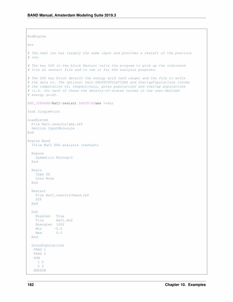
BAND Manual, Amsterdam Modeling Suite 2019.3
EndEngine
eor
# The next run has largely the same input and provides a restart of the previous# run.
# The key DOS in the block Restart tells the program to pick up the indicated# file as restart file and to use it for DOS analysis purposes.
# The DOS key block details the energy grid (and range) and the file to write# the data to. The optional keys GROSSPOPULATIONS and OverlapPopulations invoke# the computation of, respectively, gross populations and overlap populations# (i.e. for each of these the density-of-states values in the user-defined# energy grid).
AMS_JOBNAME=NaCl-restart $ADFBIN/ams <<eor
Task SinglePoint
LoadSystemFile NaCl.results/ams.rkfSection InputMolecule
End
Engine BandTitle NaCl DOS analysis (restart)
KspaceSymmetric KInteg=3
End
BasisType SZCore None
End
RestartFile NaCl.results/band.rkfSCF
End
DOSEnabled TrueFile NaCl.dosEnergies 1000Min -0.5Max 0.5
End
GrossPopulationsFRAG 1FRAG 2SUM
1 02 0
ENDSUM
182 Chapter 10. Examples

BAND Manual, Amsterdam Modeling Suite 2019.3
End
OverlapPopulationsLeftFRAG 1RightFRAG 2Left1 01 1
Right2 02 1
End
Print AtomicChargesDetailsEndEngineeor
# Finally, we copy the contents of the DOS result file to standard output
echo ""echo Contents of DOS filecat NaCl.dos
10.6.2 Example: Transition-State search using initial Hessian
Download COChainFreqTS.run
#! /bin/sh
# This example demonstrates in the first step how to calculate the Hessian.# The second run uses the pre-calculated Hessian and performs a transition# state search along the frequency mode with the smallest frequency.
# First run: Calculate Hessian# ============================
AMS_JOBNAME=hessian $ADFBIN/ams << EOF
Task SinglePoint
PropertiesHessian True
End
SystemAtoms
C 0.0 0.0 0.0O 1.5 0.5 0.0
EndLattice
3.2 0.0 0.0End
End
10.6. Structure and Reactivity 183

BAND Manual, Amsterdam Modeling Suite 2019.3
Engine BandBasis Type=DZPKSpace Quality=Good
EndEngine
EOF
# Second run: TS search with initial Hessian# ==========================================
AMS_JOBNAME=TS $ADFBIN/ams << EOF
Task TransitionStateSearch
SystemAtoms
C 0.0 0.0 0.0O 1.5 0.5 0.0
EndLattice
3.2 0.0 0.0End
End
GeometryOptimizationConvergence Gradients=1.0e-4InitialHessian
# Load the pre-calculated Hessian as the initial Hessian for the# transition state search using the Quasi-Newton based optimizer.Type FromFileFile hessian.results/band.rkf
EndEnd
Properties# Also calculate normal modes in the end, so we can see if we actually# found a transition state.NormalModes True
End
Engine BandBasis Type=DZPKSpace Quality=Good
EndEngine
EOF
10.6.3 Example: Atomic energies
Download H_ref.run
#! /bin/sh
# This example consists of several atomic energy calculations:
184 Chapter 10. Examples
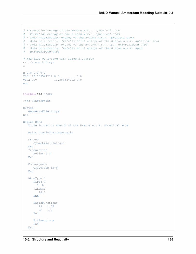
BAND Manual, Amsterdam Modeling Suite 2019.3
# - Formation energy of the H-atom w.r.t. spherical atom# - Formation energy of the H-atom w.r.t. spherical atom# - Spin polarization energy of the H-atom w.r.t. spherical atom# - Spin polarization (relativistic) energy of the H-atom w.r.t. spherical atom# - Spin polarization energy of the H-atom w.r.t. spin unrestricted atom# - Spin polarization (relativistic) energy of the H-atom w.r.t. spin# unrestricted atom
# XYZ file of H atom with large 2 latticecat << eor > H.xyz1
H 0.0 0.0 0.0VEC1 10.583544212 0.0 0.0VEC2 0.0 10.583544212 0.0eor
$ADFBIN/ams <<eor
Task SinglePoint
SystemGeometryFile H.xyz
End
Engine BandTitle Formation energy of the H-atom w.r.t. spherical atom
Print AtomicChargesDetails
KspaceSymmetric KInteg=5
EndIntegration
Accint 5.0End
ConvergenceCriterion 1E-6
End
AtomType HDirac H
1 0VALENCE
1S 1End
BasisFunctions1S 1.582P 1.0
End
FitFunctionsEnd
End
10.6. Structure and Reactivity 185
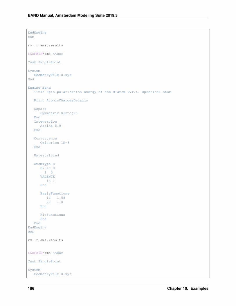
BAND Manual, Amsterdam Modeling Suite 2019.3
EndEngineeor
rm -r ams.results
$ADFBIN/ams <<eor
Task SinglePoint
SystemGeometryFile H.xyz
End
Engine BandTitle Spin polarization energy of the H-atom w.r.t. spherical atom
Print AtomicChargesDetails
KspaceSymmetric KInteg=5
EndIntegration
Accint 5.0End
ConvergenceCriterion 1E-6
End
Unrestricted
AtomType HDirac H
1 0VALENCE
1S 1End
BasisFunctions1S 1.582P 1.0
End
FitFunctionsEnd
EndEndEngineeor
rm -r ams.results
$ADFBIN/ams <<eor
Task SinglePoint
SystemGeometryFile H.xyz
186 Chapter 10. Examples

BAND Manual, Amsterdam Modeling Suite 2019.3
End
Engine BandTitle Spin polarization (relativistic) energy of the H-atom w.r.t. spherical atom
Print AtomicChargesDetails
KspaceSymmetric KInteg=5
EndIntegration
Accint 5.0End
ConvergenceCriterion 1E-6
End
Unrestricted
RelativityLevel Scalar
End
AtomType HDirac H
1 0VALENCE
1S 1End
BasisFunctions1S 1.582P 1.0
End
FitFunctionsEnd
EndEndEngineeor
rm -r ams.results
$ADFBIN/ams <<eor
Task SinglePoint
SystemGeometryFile H.xyz
End
Engine BandTitle Spin polarization energy of the H-atom w.r.t. spin unrestricted atom
Print AtomicChargesDetails
10.6. Structure and Reactivity 187

BAND Manual, Amsterdam Modeling Suite 2019.3
KspaceSymmetric KInteg=5
EndIntegration
Accint 5.0End
ConvergenceCriterion 1E-6
End
UnrestrictedUnrestrictedReference
AtomType HDirac H
1 0VALENCE
1S 1End
BasisFunctions1S 1.582P 1.0
End
FitFunctionsEnd
EndEndEngineeor
rm -r ams.results
$ADFBIN/ams <<eor
Task SinglePoint
SystemGeometryFile H.xyz
End
Engine BandTitle Spin polarization (relativistic) energy of the H-atom w.r.t. spin
→˓unrestricted atom
Print AtomicChargesDetails
KspaceSymmetric KInteg=5
EndIntegration
Accint 5.0End
ConvergenceCriterion 1E-6
188 Chapter 10. Examples

BAND Manual, Amsterdam Modeling Suite 2019.3
End
UnrestrictedReferenceUnrestricted
RelativityLevel Scalar
End
AtomType HDirac H
1 0VALENCE
1S 1End
BasisFunctions1S 1.582P 1.0
End
FitFunctionsEnd
EndEndEngineeor
10.6.4 Example: Calculating the atomic forces
Download BNForce.run
#!/bin/sh
# This example shows how to calculate the gradient of the energy with respect to# atomic displacements, using the GRADIENTS key block. For more details on# consult the documentation for Gradients.
$ADFBIN/ams <<eor
Task SinglePoint
SystemAtomsB 0.0 0.0 0.0N 0.86544 0.86544 0.86544
endLattice
0.0 1.8 1.81.8 0.0 1.81.8 1.8 0.0
EndEnd
PropertiesGradients True
End
10.6. Structure and Reactivity 189

BAND Manual, Amsterdam Modeling Suite 2019.3
Engine BandTitle BN zincblende structure (force calculation)
NumericalQuality Basic ! for speed, not very accurate
BasisType TZ2PCore Large
EndEndEngine
eor
# In the output you will find the result# FINAL GRADIENTS# 1 B 0.017517 0.017517 0.017517# 2 N -0.017517 -0.017517 -0.017517
10.6.5 Example: Optimizing the geometry
Download H2BulkGeo.run
#! /bin/sh
# This example shows how to optimize the geometry.
# This example consists of two runs. The first run performs 5 iterations# regarding the geometry optimization. And the second run exploits the# possibility to restart a geometry optimization based on the rkf of a# previous, presumably non-converged run.
# ----------------------------- first run --------------------------
AMS_JOBNAME=First $ADFBIN/ams <<eor
Task GeometryOptimization
SystemATOMS [Bohr]H 0.0 0.0 0.0H 1.0 0.0 0.0
End
Lattice [Bohr]5.0 0 00 5.0 00 0 5.0
EndEnd
GeometryOptimizationMaxIterations 5Convergence Gradients=1e-6
End
190 Chapter 10. Examples

BAND Manual, Amsterdam Modeling Suite 2019.3
Engine BandBasisType DZP
EndEndEngine
eor
# In the next run we use the result file to continue the geometry optimization.
# ----------------------------- second run --------------------------
$ADFBIN/ams <<eor
Task GeometryOptimization
LoadSystemFile First.results/ams.rkf
End
GeometryOptimizationMaxIterations 5Convergence Gradients=1e-6
End
Engine BandBasis
Type DZPEnd
EndEngineeor
echo 'Extract optimized geometry from the rkf file'$ADFBIN/adfreport ams.results/ams.rkf -r 'Molecule%Coords##3'
echo 'Extract number of steps from the rkf file'$ADFBIN/adfreport ams.results/ams.rkf -r 'History%nEntries'
10.7 Time dependent DFT
10.7.1 Example: TD-CDFT for MoS2 Monolayer (NewResponse)
Download NewResp_2DMoS2Restart.run
#!/bin/sh
# This example demonstrates how to calculate the frequency-dependent dielectric# function with the help of the NewResponse implementation for a two-dimensional# system. (see NewResponse) Furthermore, the general setup to run the TD-CDFT# section as a restart calculation is presented as well. This allows for# splitting of the frequency range into several parts, which can then be# calculated in separate calculation without the overhead of evaluating the# groundstate properties for each of them! Hence, it is a trivial
10.7. Time dependent DFT 191
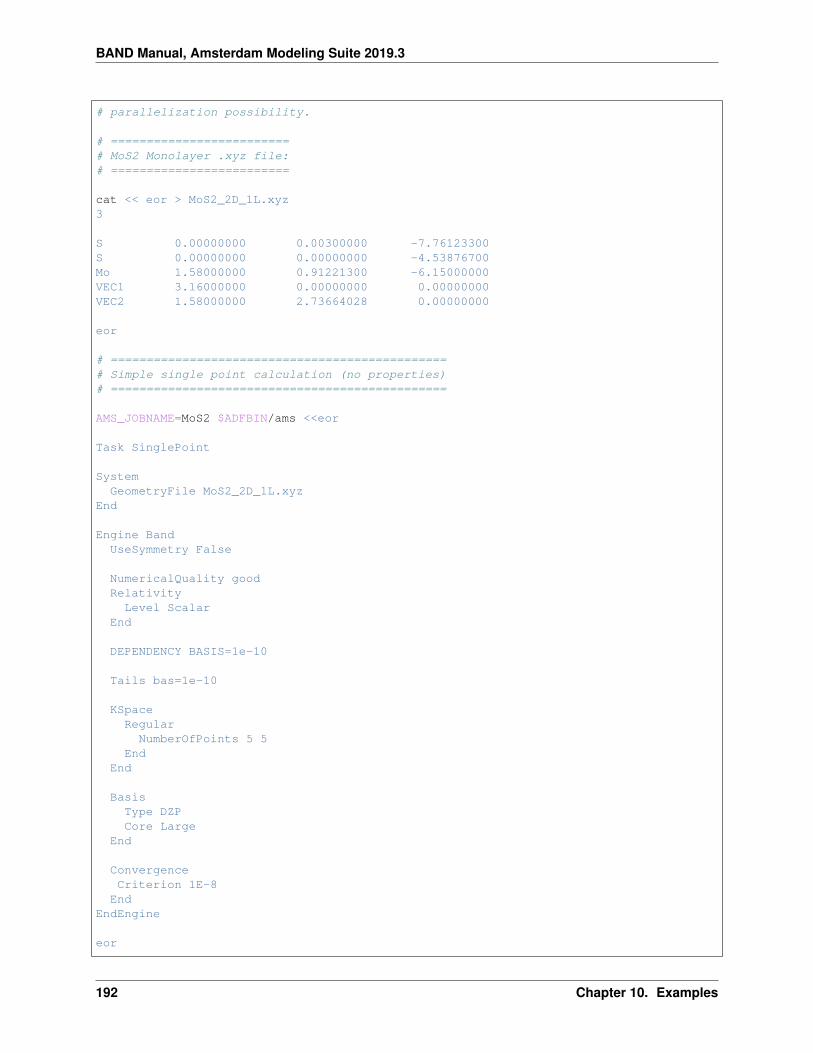
BAND Manual, Amsterdam Modeling Suite 2019.3
# parallelization possibility.
# =========================# MoS2 Monolayer .xyz file:# =========================
cat << eor > MoS2_2D_1L.xyz3
S 0.00000000 0.00300000 -7.76123300S 0.00000000 0.00000000 -4.53876700Mo 1.58000000 0.91221300 -6.15000000VEC1 3.16000000 0.00000000 0.00000000VEC2 1.58000000 2.73664028 0.00000000
eor
# ===============================================# Simple single point calculation (no properties)# ===============================================
AMS_JOBNAME=MoS2 $ADFBIN/ams <<eor
Task SinglePoint
SystemGeometryFile MoS2_2D_1L.xyz
End
Engine BandUseSymmetry False
NumericalQuality goodRelativityLevel Scalar
End
DEPENDENCY BASIS=1e-10
Tails bas=1e-10
KSpaceRegular
NumberOfPoints 5 5End
End
BasisType DZPCore Large
End
ConvergenceCriterion 1E-8End
EndEngine
eor
192 Chapter 10. Examples

BAND Manual, Amsterdam Modeling Suite 2019.3
# ===================================# Restart and compute some properties# ===================================
# Caution!# One has to make sure to use the same# Symmetry/NumericalQuality/KSpace/Basis/ZORA/... options for the# ground state calculation and for the restart calculation! Otherwise a normal# ground state SCF optimization will be performed in the restart calculation.
AMS_JOBNAME=MoS2_restart $ADFBIN/ams <<eor
Task SinglePoint
SystemGeometryFile MoS2_2D_1L.xyz
End
Engine Band
UseSymmetry False
NumericalQuality goodRelativity
Level ScalarEnd
DEPENDENCY BASIS=1e-10
Tails bas=1e-10
KSpaceRegular
NumberOfPoints 5 5End
End
BasisType DZPCore Large
End
ConvergenceCriterion 1E-8
End
RestartFile MoS2.results/band.rkfSCF
End
NewResponsenFreq 4FreqLow 2.0FreqHigh 2.7ActiveESpace 10.0
10.7. Time dependent DFT 193

BAND Manual, Amsterdam Modeling Suite 2019.3
ActiveXYZ T T FEnd
NewResponseSCFnCycle 50Criterion 1E-3
End
NewResponseKSPACEsubsimp 10eta 1e-6
EndEndEngine
eor
# ============# Extract info# ============
$ADFBIN/adfreport MoS2_restart.results/band.rkf RESPDIELRE$ADFBIN/adfreport MoS2_restart.results/band.rkf RESPDIELIM
# The results are accessible via the standard output or via the prop.kf file.# For the latter, one can use the ADFreport command $ADFBIN/adfreport prop.kf# RESPDIELRE and $ADFBIN/adfreport prop.kf RESPDIELIM to print the components# of the dielectric function for the real (RESPDIELRE) and imaginary# (RESPDIELIM) part separately. In the following tables, only the diagonal# components are presented:
# Real part# Frequency (au) epsilon_1(XX) epsilon_1(YY) epsilon_1(ZZ)# 0.0735 8.1622063 8.1788067 1.8845925# 0.0772 8.7718566 8.7960299 1.8891231# 0.0808 9.6251443 9.6631930 1.8941277# 0.0845 10.9457271 11.0126367 1.8996502# 0.0882 13.4618956 13.6001321 1.9057858# 0.0919 26.5135344 25.9300685 1.9126665# 0.0955 6.1134118 4.1756368 1.9204849# 0.0992 6.2789015 4.6880515 1.9295347# 0.1029 13.7665058 11.5484340 1.9403044# 0.1066 -7.2575153 -5.8285172 1.9537079# 0.1102 -0.7937277 1.2661253 1.9718981
# Imaginary part# Frequency (au) epsilon_2(XX) epsilon_2(YY) epsilon_2(ZZ)# 0.0735 0.0015601 0.0015758 0.0000213# 0.0772 0.0020566 0.0020839 0.0000200# 0.0808 0.0029274 0.0029798 0.0000216# 0.0845 0.0047632 0.0048794 0.0000231# 0.0882 0.0104743 0.0107877 0.0000246# 0.0919 0.2658531 0.1942899 0.0000264# 0.0955 12.8856772 14.5286319 0.0000294# 0.0992 9.7571573 10.1567455 0.0000338# 0.1029 7.5936072 6.7674596 0.0000399# 0.1066 13.0264038 9.5897946 0.0000487# 0.1102 0.2483041 0.3222301 0.0000676
194 Chapter 10. Examples
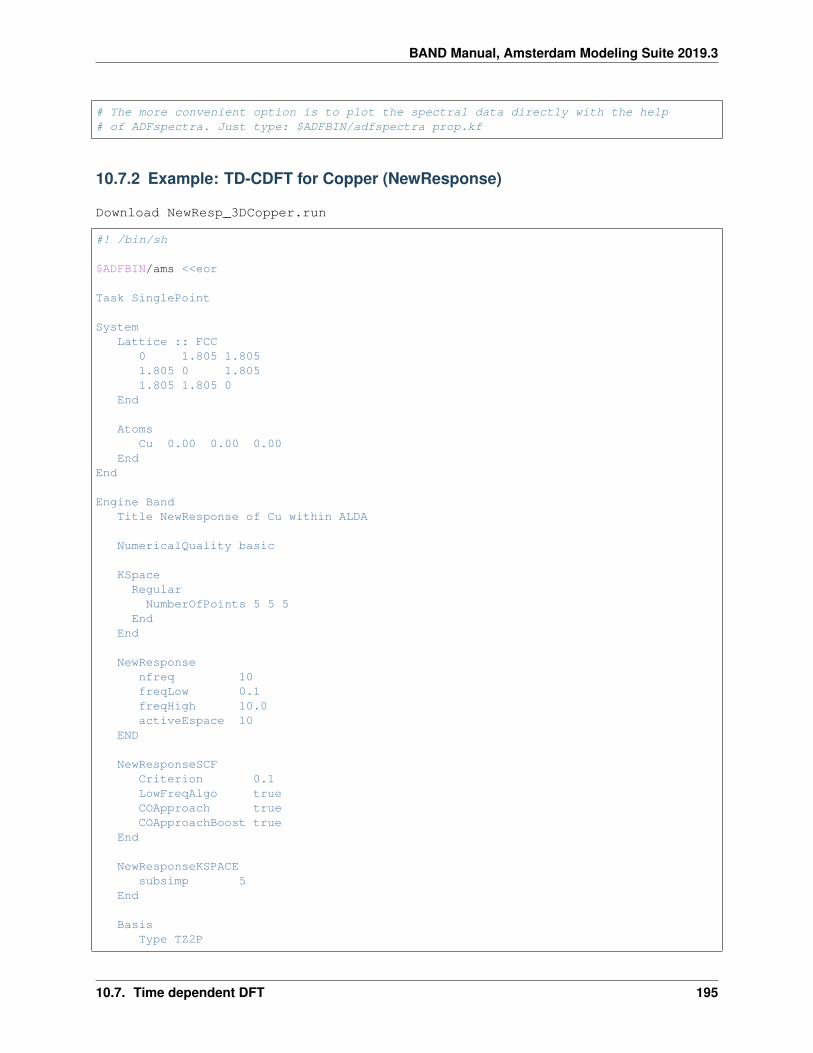
BAND Manual, Amsterdam Modeling Suite 2019.3
# The more convenient option is to plot the spectral data directly with the help# of ADFspectra. Just type: $ADFBIN/adfspectra prop.kf
10.7.2 Example: TD-CDFT for Copper (NewResponse)
Download NewResp_3DCopper.run
#! /bin/sh
$ADFBIN/ams <<eor
Task SinglePoint
SystemLattice :: FCC
0 1.805 1.8051.805 0 1.8051.805 1.805 0
End
AtomsCu 0.00 0.00 0.00
EndEnd
Engine BandTitle NewResponse of Cu within ALDA
NumericalQuality basic
KSpaceRegular
NumberOfPoints 5 5 5End
End
NewResponsenfreq 10freqLow 0.1freqHigh 10.0activeEspace 10
END
NewResponseSCFCriterion 0.1LowFreqAlgo trueCOApproach trueCOApproachBoost true
End
NewResponseKSPACEsubsimp 5
End
BasisType TZ2P
10.7. Time dependent DFT 195
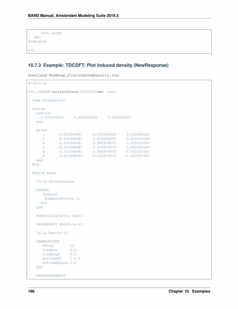
BAND Manual, Amsterdam Modeling Suite 2019.3
Core LargeEnd
EndEngine
eor
10.7.3 Example: TDCDFT: Plot induced density (NewResponse)
Download NewResp_PlotInducedDensity.run
#!/bin/sh
AMS_JOBNAME=polyethylene $ADFBIN/ams <<eor
Task SinglePoint
SystemLattice
2.553395923 0.000000000 0.000000000end
AtomsC -0.623348981 -0.055000000 0.425969423C 0.633348981 0.015000000 -0.422636089H -0.633348981 0.964974570 1.055290696H -0.623348981 -0.914974570 1.055290696H 0.633348981 0.904974570 -1.051957363H 0.613348981 -0.914974570 -1.061957363
endEnd
Engine Band
Title Polyethylene
KSPACERegularNumberOfPoints 11
EndEnd
NumericalQuality basic
DEPENDENCY BASIS=1e-10
Tails bas=1e-10
NEWRESPONSEnFreq 10FreqLow 6.0FreqHigh 8.0ActiveXYZ T F FActiveESpace 2.0
END
NEWRESPONSESCF
196 Chapter 10. Examples
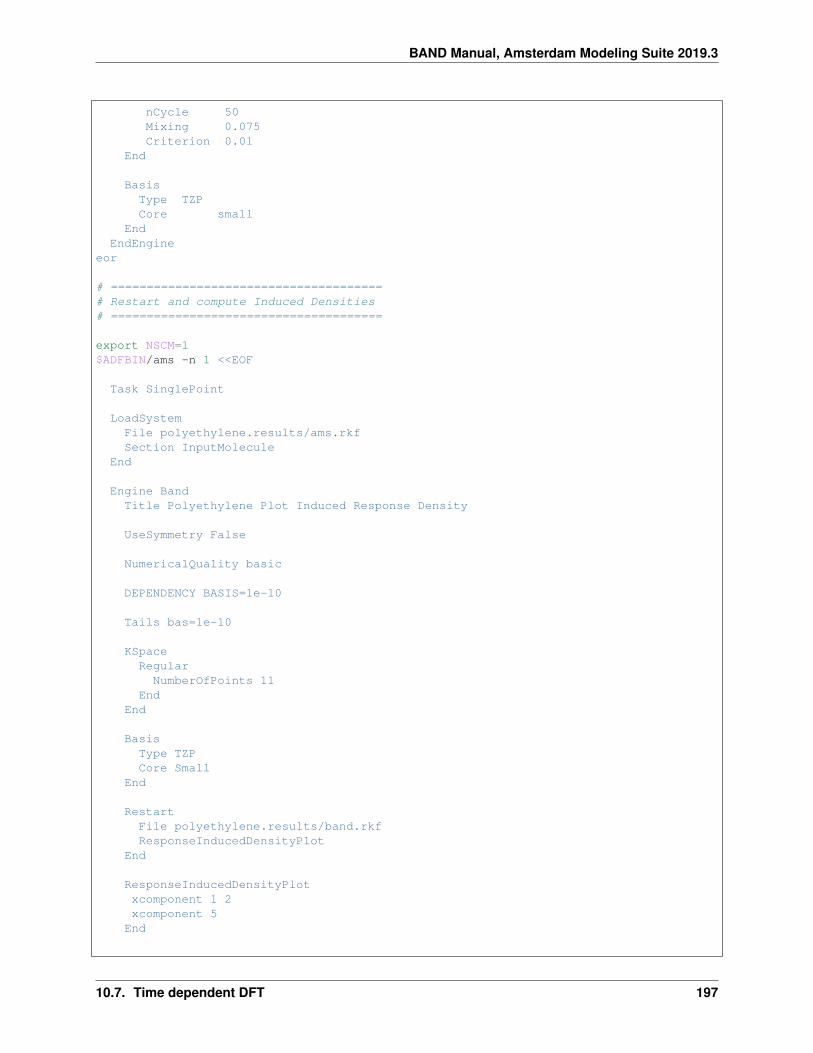
BAND Manual, Amsterdam Modeling Suite 2019.3
nCycle 50Mixing 0.075Criterion 0.01
End
BasisType TZPCore small
EndEndEngine
eor
# ======================================# Restart and compute Induced Densities# ======================================
export NSCM=1$ADFBIN/ams -n 1 <<EOF
Task SinglePoint
LoadSystemFile polyethylene.results/ams.rkfSection InputMolecule
End
Engine BandTitle Polyethylene Plot Induced Response Density
UseSymmetry False
NumericalQuality basic
DEPENDENCY BASIS=1e-10
Tails bas=1e-10
KSpaceRegular
NumberOfPoints 11End
End
BasisType TZPCore Small
End
RestartFile polyethylene.results/band.rkfResponseInducedDensityPlot
End
ResponseInducedDensityPlotxcomponent 1 2xcomponent 5
End
10.7. Time dependent DFT 197

BAND Manual, Amsterdam Modeling Suite 2019.3
GridEnd
debug BlockPropertyModuleEndEngine
EOF
echo ""echo "Begin TOC of tape41"export NSCM=1$ADFBIN/pkf -n 1 ams.results/FILE_BLOCKPROPERTIESecho "End TOC of tape41"
10.7.4 Example: TD-CDFT for bulk diamond (OldResponse)
Download OldResp_Diamond.run
#! /bin/sh
# Response calculation for diamond
$ADFBIN/ams <<eor
Task SinglePoint
SystemLATTICE
0 1.785 1.7851.785 0 1.7851.785 1.785 0
ENDATOMS
C 0.0 0.0 0.0C 0.8925 0.8925 0.8925
ENDEnd
Engine BandTITLE DIAMOND
IntegrationAccint 5
End
KSPACESymmetric KInteg=2
End
Dependency Basis=1.e-6
OLDRESPONSEEnabled Truenfreq 7strtfr 0.0endfr 19.0480
END
198 Chapter 10. Examples

BAND Manual, Amsterdam Modeling Suite 2019.3
BasisType DZ
EndEndEngine
eor
10.8 Spectroscopy
10.8.1 Example: Hyperfine A-tensor
Download TiF3a.run
#!/bin/sh
# Example for an ESR A-tensor calculation.
# Be aware that the calculation must be spin unrestricted and the ATENSOR# keyword must be present, too.
$ADFBIN/ams <<eor
Task SinglePoint
SystemAtoms
Ti 0.0 0.0 0.0F 1.78 0.0 0.0F -0.89 1.541525218736 0.0F -0.89 -1.541525218736 0.0
endEnd
Engine BandTitle TiF3
Unrestricted True
EFGEnabled True
End
ATensorEnabled True
End
BasisType TZPCore None
EndEndEngineeor
10.8. Spectroscopy 199

BAND Manual, Amsterdam Modeling Suite 2019.3
10.8.2 Example: Zeeman g-tensor
Download TiF3g.run
#!/bin/sh
# Example for an ESR g-tensor calculation. More information in the documentation# of ESR
# Be aware that this calculation must include the spin-orbit, relativistic# approximation (Relativistic ZORA Spin)!
$ADFBIN/ams <<eor
Task SinglePoint
SystemAtoms
Ti 0.0 0.0 0.0F 0.0 1.78 0.0F -1.541525218736 -0.89 0.0F 1.541525218736 -0.89 0.0
endEnd
Engine BandTitle TiF3
RelativityLevel Spin-Orbit
End
ESREnabled True
end
BasisType DZCore None
EndEndEngine
eor
10.8.3 Example: NMR
Download PE-NMR.run
#! /bin/sh
# With the NMR key block you can specify for which atom you want the shielding# tensor.
# Be aware that the NMR option is not implemented for the frozen core# approximation, hence one must set option core of the Basis key block# to NONE.
200 Chapter 10. Examples

BAND Manual, Amsterdam Modeling Suite 2019.3
$ADFBIN/ams <<eor
Task SinglePoint
SystemAtoms
C -0.638348981 0.000000000 0.424302756C 0.638348981 0.000000000 -0.424302756H -0.638348981 0.889974570 1.053624029H -0.638348981 -0.889974570 1.053624029H 0.638348981 0.889974570 -1.053624029H 0.638348981 -0.889974570 -1.053624029
End
Lattice2.553395923 0.000000000 0.000000000
endEnd
Engine BandNMR
Enabled Truenmratom 1ms0 1.
end
XCGGA Always Becke Perdew
end
DependencyBasis 1e-10
End
KspaceSymmetric KInteg=3
EndIntegration
Accint 5End
BasisType TZ2PCore NONE
EndEndEngine
eor
10.8.4 Example: EFG
Download SnO_EFG.run
#!/bin/sh
# The calculation of the electric field gradient is invoked by the EFG key
10.8. Spectroscopy 201

BAND Manual, Amsterdam Modeling Suite 2019.3
# block.
# Since Sn is quite an heavy atom we use the scalar relativistic option.
$ADFBIN/ams <<eor
Task SinglePoint
SystemFractionalCoords True
Lattice3.8029 0.0 0.00.0 3.8029 0.00.0 0.0 4.8382
End
AtomsO 0.0 0.0 0.0O 0.5 0.5 0.0Sn 0.0 0.5 0.2369Sn 0.5 0.0 -0.2369
EndEnd
Engine BandTitle SnO EFG
NumericalQuality Basic ! Only for speed
Tails bas=1e-8 ! Only for reproducibility with nr. of cores
RelativityLevel Scalar
End
! useful for Moessbauer spectroscopy: density and coulomb pot. at nucleiPropertiesAtNucleiEnd
EFGEnabled True
End
BasisType DZCore none
EndEndEngineeor
10.8.5 Example: Phonons
Download GraphenePhonons.run
202 Chapter 10. Examples

BAND Manual, Amsterdam Modeling Suite 2019.3
#!/bin/sh
# A phonon calculation should be performed at the equilibrium geometry.
# In the first calculation we optimize the geometry, including the lattice# vectors. We also set the criteria a bit more strict.
echo "Geometry optimization"
AMS_JOBNAME=GO $ADFBIN/ams <<eor
SystemAtomsC 0.0 0.0 0.0C 1.23 0.7101408312 0.0
ENDLattice2.46 0.000000 01.23 2.130422493 0
EndEnd
Task GeometryOptimization
GeometryOptimizationOptimizeLattice trueConvergence Gradients=1e-5Method Quasi-Newton
End
Engine BandTitle Graphene geometry optimization
! For Graphene we need to use a symmetric gridKSpaceSymmetric KInteg=5Type Symmetric
End
StrainDerivativesAnalytical false
End
BasisType DZ
endEndEngineeor
# In the second calculation we use the pre-optimized geometry. (See details of# the Restart key block) Then we define a supercell and perform a phonon run by# using Task and Phonons keys. Note that KSpace can be chosen# a bit lower, since we now have a bigger unit cell.
echo "Phonon calculation"
AMS_JOBNAME=Phonons $ADFBIN/ams <<eor
10.8. Spectroscopy 203

BAND Manual, Amsterdam Modeling Suite 2019.3
LoadSystemFile GO.results/ams.rkf
End
Task SinglePoint
PropertiesPhonons True
End
NumericalPhononsstepSize 0.0913SuperCell2 00 2
Endend
Engine BandTitle Graphene phonon calc
KSpaceSymmetric KInteg=3Type Symmetric
End
BasisType DZ
endEndEngine
eor
NSCM=1export NSCMecho ""echo "Begin TOC"
$ADFBIN/dmpkf -n 1 Phonons.results/band.rkf --toc
echo "End TOC"
10.9 Analysis
10.9.1 Example: CO absorption on a Cu slab: fragment option and densityplot
Download Frags_COCu.run
#! /bin/sh
# This example illustrates the usage of fragments in a BAND calculation for# analysis purposes. It takes two runs to do the DOS analysis in a fragment# basis, and an extra two runs to get the deformation density with respect to# the fragment densities.
204 Chapter 10. Examples

BAND Manual, Amsterdam Modeling Suite 2019.3
# The setup involves first the computation of the free CO overlayer, which is to# be adsorbed on a Cu surface. To suppress (most of the) interactions between# the CO molecules, i.e. to effectively get the molecular CO, the KSpace# parameter is set to 1 (= no dispersion), and the lattice parameters are set so# large that the CO molecules are far apart. The standard result file RUNKF is# saved under the name 'CO.results/band.rkf'.
# ----------------------------- CO molecule --------------------------
AMS_JOBNAME=CO $ADFBIN/ams <<eor
Task SinglePoint
System! CO molecules far apart
Atoms [Bohr]C 0 0 0O 0 0 2.18
End
Lattice [Bohr]25.0 0.0 0.00.0 25.0 0.0
EndEnd
Engine BandTitle The CO fragment
Print AtomicChargesDetails
CommentTechnical
Zero order k space integrationFeatures
Lattice : 2D, large lattice vectorsUnit cell : 2 atoms, 1x1, quasi molecularBasis : NO+STO w/ core
End
Print Eigens
KspaceQuality GammaOnly ! neglect dispersion
End
BasisType DZCore Large
End
DOSEnabled TrueEnergies 300
EndEndEngine
10.9. Analysis 205

BAND Manual, Amsterdam Modeling Suite 2019.3
eor
# Now we can use the result file to do a DOS analysis for CO on a copper surface# treating the molecule as a fragment. With Fragment%Labels we assign names to# the different symmetry orbitals. The Density-of-States analysis details are# given with the keys DOS (energy grid, result file with DOS data) and,# optionally, GrossPopulations and OverlapPopulations.
# ----------------------------- CO + Cu slab --------------------------
AMS_JOBNAME=COCu $ADFBIN/ams <<eor
Task SinglePoint
SystemLattice [Bohr]4.822 0.0 0.00.0 4.822 0.0
EndAtoms [Bohr]C 0 0 3.44O 0 0 5.62Cu 0.0 0.0 0.0
EndEnd
Engine BandTitle Cu slab with CO adsorbed
Print AtomicChargesDetails
CommentTechnical
Quadratic K space integration (low)Features
Lattice : 2DUnit cell : 3 atoms, 1x1Basis : NO+STO w/ coreOptions : Molecular fragment
Analysis: DOS, PDOS, COOPEnd
KSpaceSymmetric KInteg=3
End
! fragment specification
Fragmentfilename CO.results/band.rkfatommapping
1 12 2
EndLabels ! let us give them some labels
2Sigma2Sigma*
206 Chapter 10. Examples
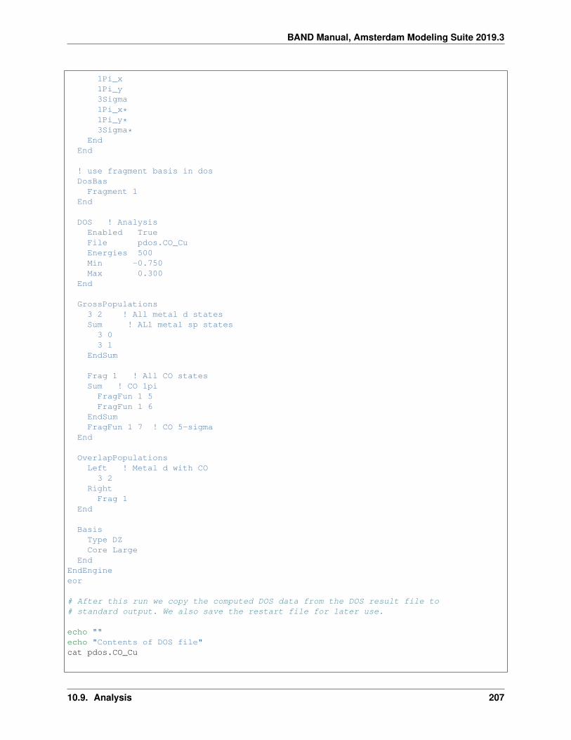
BAND Manual, Amsterdam Modeling Suite 2019.3
1Pi_x1Pi_y3Sigma1Pi_x*1Pi_y*3Sigma*
EndEnd
! use fragment basis in dosDosBasFragment 1
End
DOS ! AnalysisEnabled TrueFile pdos.CO_CuEnergies 500Min -0.750Max 0.300
End
GrossPopulations3 2 ! All metal d statesSum ! ALl metal sp states
3 03 1
EndSum
Frag 1 ! All CO statesSum ! CO 1pi
FragFun 1 5FragFun 1 6
EndSumFragFun 1 7 ! CO 5-sigma
End
OverlapPopulationsLeft ! Metal d with CO
3 2Right
Frag 1End
BasisType DZCore Large
EndEndEngineeor
# After this run we copy the computed DOS data from the DOS result file to# standard output. We also save the restart file for later use.
echo ""echo "Contents of DOS file"cat pdos.CO_Cu
10.9. Analysis 207
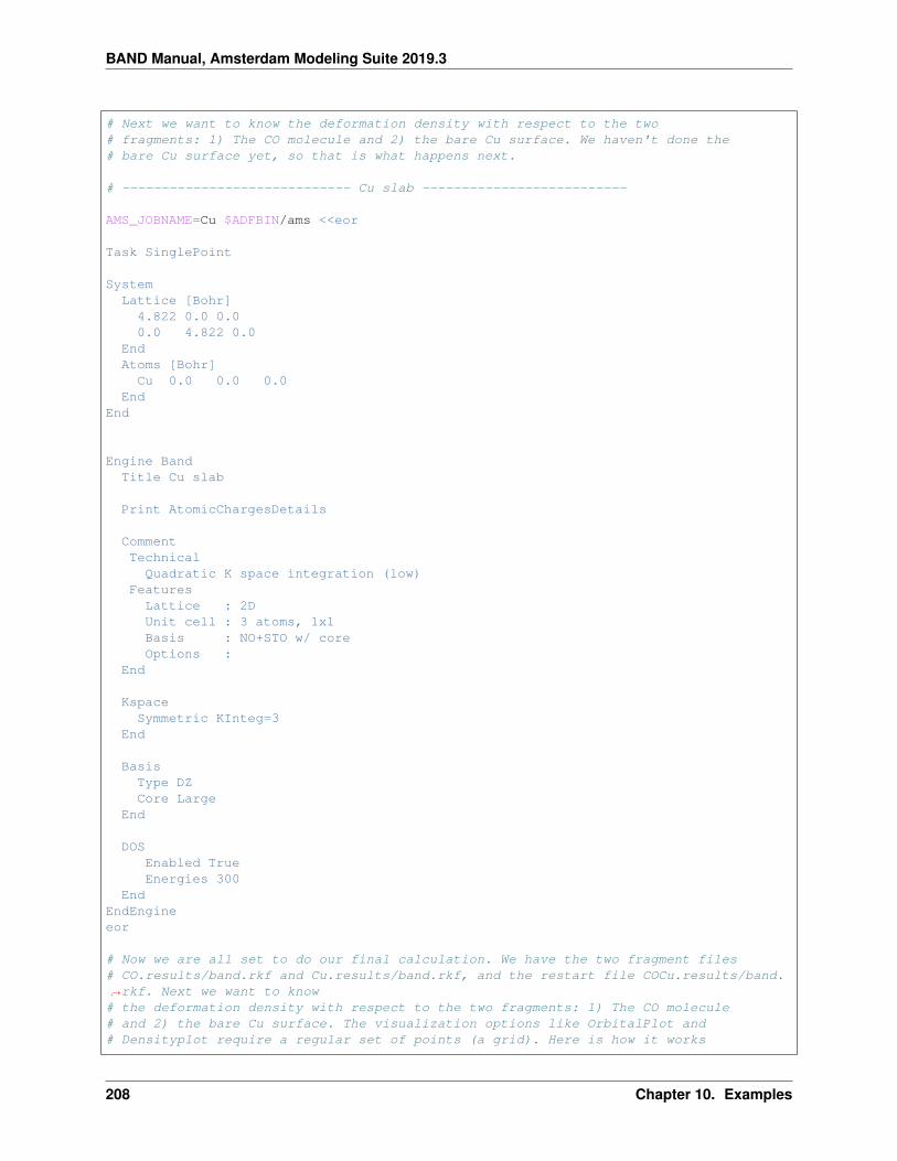
BAND Manual, Amsterdam Modeling Suite 2019.3
# Next we want to know the deformation density with respect to the two# fragments: 1) The CO molecule and 2) the bare Cu surface. We haven't done the# bare Cu surface yet, so that is what happens next.
# ----------------------------- Cu slab --------------------------
AMS_JOBNAME=Cu $ADFBIN/ams <<eor
Task SinglePoint
SystemLattice [Bohr]4.822 0.0 0.00.0 4.822 0.0
EndAtoms [Bohr]Cu 0.0 0.0 0.0
EndEnd
Engine BandTitle Cu slab
Print AtomicChargesDetails
CommentTechnical
Quadratic K space integration (low)Features
Lattice : 2DUnit cell : 3 atoms, 1x1Basis : NO+STO w/ coreOptions :
End
KspaceSymmetric KInteg=3
End
BasisType DZCore Large
End
DOSEnabled TrueEnergies 300
EndEndEngineeor
# Now we are all set to do our final calculation. We have the two fragment files# CO.results/band.rkf and Cu.results/band.rkf, and the restart file COCu.results/band.→˓rkf. Next we want to know# the deformation density with respect to the two fragments: 1) The CO molecule# and 2) the bare Cu surface. The visualization options like OrbitalPlot and# Densityplot require a regular set of points (a grid). Here is how it works
208 Chapter 10. Examples
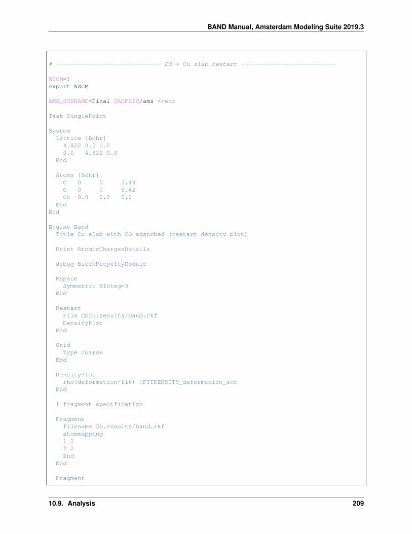
BAND Manual, Amsterdam Modeling Suite 2019.3
# ----------------------------- CO + Cu slab restart --------------------------
NSCM=1export NSCM
AMS_JOBNAME=Final $ADFBIN/ams <<eor
Task SinglePoint
SystemLattice [Bohr]4.822 0.0 0.00.0 4.822 0.0
End
Atoms [Bohr]C 0 0 3.44O 0 0 5.62Cu 0.0 0.0 0.0
EndEnd
Engine BandTitle Cu slab with CO adsorbed (restart density plot)
Print AtomicChargesDetails
debug BlockPropertyModule
KspaceSymmetric KInteg=3
End
RestartFile COCu.results/band.rkfDensityPlot
End
GridType Coarse
End
DensityPlotrho(deformation/fit) !FITDENSITY_deformation_scf
End
! fragment specification
Fragmentfilename CO.results/band.rkfatommapping1 12 2End
End
Fragment
10.9. Analysis 209
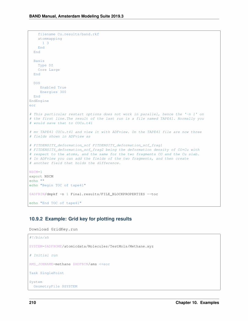
BAND Manual, Amsterdam Modeling Suite 2019.3
filename Cu.results/band.rkfatommapping
1 3End
End
BasisType DZCore Large
End
DOSEnabled TrueEnergies 300
EndEndEngineeor
# This particular restart options does not work in parallel, hence the '-n 1' on# the first line.The result of the last run is a file named TAPE41. Normally you# would save that to COCu.t41
# mv TAPE41 COCu.t41 and view it with ADFview. On the TAPE41 file are now three# fields shown in ADFview as
# FITDENSITY_deformation_scf FITDENSITY_deformation_scf_frag1# FITDENSITY_deformation_scf_frag2 being the deformation density of CO+Cu with# respect to the atoms, and the same for the two fragments CO and the Cu slab.# In ADFview you can add the fields of the two fragments, and then create# another field that holds the difference.
NSCM=1export NSCMecho ""echo "Begin TOC of tape41"
$ADFBIN/dmpkf -n 1 Final.results/FILE_BLOCKPROPERTIES --toc
echo "End TOC of tape41"
10.9.2 Example: Grid key for plotting results
Download GridKey.run
#!/bin/sh
SYSTEM=$ADFHOME/atomicdata/Molecules/TestMols/Methane.xyz
# Initial run
AMS_JOBNAME=methane $ADFBIN/ams <<eor
Task SinglePoint
SystemGeometryFile $SYSTEM
210 Chapter 10. Examples

BAND Manual, Amsterdam Modeling Suite 2019.3
End
Engine BandBasisType TZP
EndEndEngineeor
# Use the grid
AMS_JOBNAME=auto_grid $ADFBIN/ams <<eor
Task SinglePoint
SystemGeometryFile $SYSTEM
End
Engine BandRestartFile methane.results/band.rkfDensityPlot
End
GridType CoarseExtendX 21.1671 [Angstrom]End
DensityPlotrho(fit)
End
BasisType TZP
EndEndEngineeor
echo ""echo "Begin TOC of tape41"
$ADFBIN/dmpkf -n 1 auto_grid.results/TAPE41 --toc
echo "End TOC of tape41"
# Use a completely user specified regular grid
AMS_JOBNAME=user_grid $ADFBIN/ams <<eor
Task SinglePoint
10.9. Analysis 211

BAND Manual, Amsterdam Modeling Suite 2019.3
SystemGeometryFile $SYSTEM
End
Engine BandRestartFile methane.results/band.rkfDensityPlot
End
GridUserDefined
-2.0 -1.3 -2.51.0 0.0 0.0 0.020 1 0.0 0.020.0 0.0 1.0 0.0220 30 40
EndEnd
DensityPlotrho(fit)
End
BasisType TZP
EndEndEngineeor
echo ""echo "Begin TOC of tape41"
$ADFBIN/dmpkf -n 1 user_grid.results/TAPE41 --toc
echo "End TOC of tape41"
# Use a text file to import the (arbitrary grid)
cat << eor > coords.txt-3.0 0.0 0.0-2.0 0.1 0.00.0 0.2 0.0
eor
AMS_JOBNAME=file_grid $ADFBIN/ams <<eor
Task SinglePoint
SystemGeometryFile $SYSTEM
End
Engine BandRestartFile methane.results/band.rkfDensityPlot
212 Chapter 10. Examples
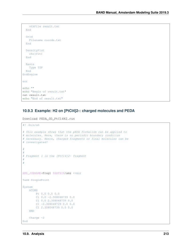
BAND Manual, Amsterdam Modeling Suite 2019.3
vtkFile result.txtEnd
GridFilename coords.txt
End
DensityPlotrho(fit)
End
BasisType TZP
EndEndEngine
eor
echo ""echo "Begin of result.txt"cat result.txtecho "End of result.txt"
10.9.3 Example: H2 on [PtCl4]2-: charged molecules and PEDA
Download PEDA_0D_PtCl4H2.run
#! /bin/sh
# This example shows that the pEDA formalism can be applied to# molecules. Here, there is no periodic boundary condition# necessary. Hence, charged fragments or final molecules can be# investigated!
### Fragment 1 is the [PtCl4]2- fragment##
AMS_JOBNAME=Frag1 $ADFBIN/ams <<eor
Task SinglePoint
SystemATOMS
Pt 0.0 0.0 0.0Cl 0.0 -2.308048739 0.0Cl 0.0 2.308048739 0.0Cl -2.308048739 0.0 0.0Cl 2.308048739 0.0 0.0
END
Charge -2End
10.9. Analysis 213

BAND Manual, Amsterdam Modeling Suite 2019.3
Engine BandTITLE PtCl4 2- fragmentRelativity
Level ScalarEnd
BasisType DZPCore LargeEnd
XCGGA Becke PerdewEND
UseSymmetry FalseEndEngineeor
### Fragment 2 is the H2 fragment##
AMS_JOBNAME=Frag2 $ADFBIN/ams <<eor
Task SinglePoint
SystemATOMS
H 0.0 0.0 3.84182655H 0.0 0.0 2.952808836
ENDEnd
Engine BandTITLE H2 fragment
RelativityLevel Scalar
End
BasisType DZPCore LargeEnd
XCGGA Becke PerdewEND
UseSymmetry FalseEndEngineeor
214 Chapter 10. Examples

BAND Manual, Amsterdam Modeling Suite 2019.3
### The energy decomposition run for the complex ([PtCl4]H2)2- complex##
$ADFBIN/ams <<eor
Task SinglePoint
SystemATOMS
Pt 0.0 0.0 0.0Cl 0.0 -2.308048739 0.0Cl 0.0 2.308048739 0.0Cl -2.308048739 0.0 0.0Cl 2.308048739 0.0 0.0H 0.0 0.0 2.952808836H 0.0 0.0 3.84182655
ENDCharge -2
End
Engine BandRelativity
Level ScalarEnd
BasisType DZPCore LargeEnd
XCGGA Becke PerdewEND
fragmentfilename Frag1.results/band.rkfAtomMapping
1 12 23 34 45 5
Endend
fragmentfilename Frag2.results/band.rkfAtomMapping
1 72 6
Endend
PEDA
10.9. Analysis 215

BAND Manual, Amsterdam Modeling Suite 2019.3
UseSymmetry FalseEndEngine
eor
10.9.4 Example: CO absorption on a MgO slab: fragment option and PEDA
Download PEDA_MgO+CO.run
#! /bin/sh
# This example shall illustrate the use of the Fragment keywords in combination# with the PEDA keyword to perform the PEDA. For this example two fragment# calculations are necessary to calculate the unperturbed eigensystems of the# MgO slab and CO fragment.
# == Fragment calculations ==
# ------------------------------ MgO slab ------------------------
AMS_JOBNAME=MgO $ADFBIN/ams <<eor
Task SinglePoint
SystemAtoms
Mg 0.00000000 0.00000000 0.00000000Mg 1.50260191 -1.50260191 -2.12400000Mg 0.00000000 0.00000000 -4.24800000Mg 3.00520382 0.00000000 0.00000000Mg 1.50260191 1.50260191 -2.12400000Mg 3.00520382 0.00000000 -4.24800000O 1.50260191 -1.50260191 0.00200000O 0.00000000 0.00000000 -2.12400000O 1.50260191 -1.50260191 -4.25000000O 1.50260191 1.50260191 0.00200000O 3.00520382 0.00000000 -2.12400000O 1.50260191 1.50260191 -4.25000000
End
Lattice3.00520382 -3.00520382 0.000000003.00520382 3.00520382 0.00000000
EndEnd
Engine BandTitle MgO surface
skip dos
KSpaceRegular
NumberOfPoints 3 3End
End
216 Chapter 10. Examples
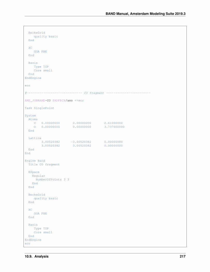
BAND Manual, Amsterdam Modeling Suite 2019.3
BeckeGridquality basic
End
XCGGA PBE
End
BasisType TZPCore small
EndEndEngine
eor
#------------------------------ CO fragment ------------------------
AMS_JOBNAME=CO $ADFBIN/ams <<eor
Task SinglePoint
SystemAtoms
C 0.00000000 0.00000000 2.61000000O 0.00000000 0.00000000 3.737000000
End
Lattice3.00520382 -3.00520382 0.000000003.00520382 3.00520382 0.00000000
EndEnd
Engine BandTitle CO fragment
KSpaceRegular
NumberOfPoints 3 3End
End
BeckeGridquality basic
End
XCGGA PBE
End
BasisType TZPCore small
EndEndEngineeor
10.9. Analysis 217

BAND Manual, Amsterdam Modeling Suite 2019.3
# == PEDA calculation ==
# The two result files, MgO.kf and CO.kf, can now be used to perform the# PEDA. Here, the mapping of the atoms of the PEDA calculation and the fragment# calculations is necessary. And the used grid points in reciprocal space have# to be identical in all three calculations.
# ----------------------------- PEDA calculation ------------------------
$ADFBIN/ams <<eor
Task SinglePoint
SystemAtoms
Mg.frag_MgO 0.00000000 0.00000000 0.00000000Mg.frag_MgO 1.50260191 -1.50260191 -2.12400000Mg.frag_MgO 0.00000000 0.00000000 -4.24800000Mg.frag_MgO 3.00520382 0.00000000 0.00000000Mg.frag_MgO 1.50260191 1.50260191 -2.12400000Mg.frag_MgO 3.00520382 0.00000000 -4.24800000O.frag_MgO 1.50260191 -1.50260191 0.00200000O.frag_MgO 0.00000000 0.00000000 -2.12400000O.frag_MgO 1.50260191 -1.50260191 -4.25000000O.frag_MgO 1.50260191 1.50260191 0.00200000O.frag_MgO 3.00520382 0.00000000 -2.12400000O.frag_MgO 1.50260191 1.50260191 -4.25000000O.frag_CO 0.00000000 0.00000000 3.73700000C.frag_CO 0.00000000 0.00000000 2.61000000
End
Lattice3.00520382 -3.00520382 0.000000003.00520382 3.00520382 0.00000000
EndEnd
Engine BandTitle PEDA
KSpaceRegular
NumberOfPoints 3 3End
End
BeckeGridquality basic
End
XCGGA PBE
End
fragmentfilename MgO.results/band.rkfAtomMapping
218 Chapter 10. Examples
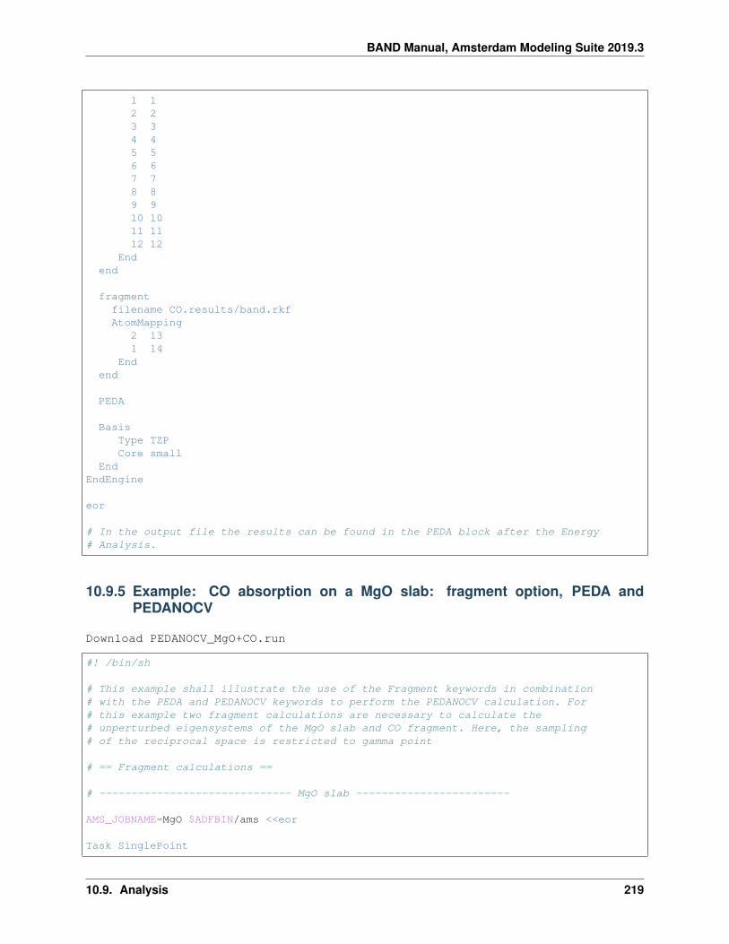
BAND Manual, Amsterdam Modeling Suite 2019.3
1 12 23 34 45 56 67 78 89 910 1011 1112 12
Endend
fragmentfilename CO.results/band.rkfAtomMapping
2 131 14
Endend
PEDA
BasisType TZPCore small
EndEndEngine
eor
# In the output file the results can be found in the PEDA block after the Energy# Analysis.
10.9.5 Example: CO absorption on a MgO slab: fragment option, PEDA andPEDANOCV
Download PEDANOCV_MgO+CO.run
#! /bin/sh
# This example shall illustrate the use of the Fragment keywords in combination# with the PEDA and PEDANOCV keywords to perform the PEDANOCV calculation. For# this example two fragment calculations are necessary to calculate the# unperturbed eigensystems of the MgO slab and CO fragment. Here, the sampling# of the reciprocal space is restricted to gamma point
# == Fragment calculations ==
# ------------------------------ MgO slab ------------------------
AMS_JOBNAME=MgO $ADFBIN/ams <<eor
Task SinglePoint
10.9. Analysis 219

BAND Manual, Amsterdam Modeling Suite 2019.3
SystemAtoms
Mg 0.00000000 0.00000000 0.00000000Mg 1.50260191 -1.50260191 -2.12400000Mg 0.00000000 0.00000000 -4.24800000Mg 3.00520382 0.00000000 0.00000000Mg 1.50260191 1.50260191 -2.12400000Mg 3.00520382 0.00000000 -4.24800000O 1.50260191 -1.50260191 0.00200000O 0.00000000 0.00000000 -2.12400000O 1.50260191 -1.50260191 -4.25000000O 1.50260191 1.50260191 0.00200000O 3.00520382 0.00000000 -2.12400000O 1.50260191 1.50260191 -4.25000000
End
Lattice3.00520382 -3.00520382 0.000000003.00520382 3.00520382 0.00000000
EndEnd
Engine BandTitle MgO fragment
skip dos
KSpaceRegular
NumberOfPoints 1 1End
End
BeckeGridquality basic
End
RelativityLevel Scalar
End
XCGGA PBE
End
BasisType TZPCore none
EndEndEngineeor
#------------------------------ CO fragment ------------------------
AMS_JOBNAME=CO $ADFBIN/ams <<eor
Task SinglePoint
220 Chapter 10. Examples

BAND Manual, Amsterdam Modeling Suite 2019.3
SystemAtoms
C 0.00000000 0.00000000 2.61000000O 0.00000000 0.00000000 3.737000000
End
Lattice3.00520382 -3.00520382 0.000000003.00520382 3.00520382 0.00000000
EndEnd
Engine BandTitle CO fragment
KSpaceRegular
NumberOfPoints 1 1End
End
BeckeGridquality basic
End
RelativityLevel Scalar
End
XCGGA PBE
End
BasisType TZPCore none
EndEndEngineeor
# == PEDANOCV calculation ==
# The two result files, MgO.kf and CO.kf, can now be used to perform the# PEDANOCV. Here, the mapping of the atoms of the PEDA calculation and the# fragment calculations is necessary. And the used grid points in reciprocal# space have to be identical in all three calculations - in this case the gamma# point for all calculations.
#------------------------------ PEDANOCV calculation ------------------------
AMS_JOBNAME=decomp $ADFBIN/ams <<eor
Task SinglePoint
SystemAtoms
10.9. Analysis 221

BAND Manual, Amsterdam Modeling Suite 2019.3
Mg.frag_MgO 0.00000000 0.00000000 0.00000000Mg.frag_MgO 1.50260191 -1.50260191 -2.12400000Mg.frag_MgO 0.00000000 0.00000000 -4.24800000Mg.frag_MgO 3.00520382 0.00000000 0.00000000Mg.frag_MgO 1.50260191 1.50260191 -2.12400000Mg.frag_MgO 3.00520382 0.00000000 -4.24800000O.frag_MgO 1.50260191 -1.50260191 0.00200000O.frag_MgO 0.00000000 0.00000000 -2.12400000O.frag_MgO 1.50260191 -1.50260191 -4.25000000O.frag_MgO 1.50260191 1.50260191 0.00200000O.frag_MgO 3.00520382 0.00000000 -2.12400000O.frag_MgO 1.50260191 1.50260191 -4.25000000C.frag_CO 0.00000000 0.00000000 2.61000000O.frag_CO 0.00000000 0.00000000 3.737000000
End
Lattice3.00520382 -3.00520382 0.000000003.00520382 3.00520382 0.00000000
EndEnd
Engine BandTitle Mg+CO
KSpaceRegular
NumberOfPoints 1 1End
End
BeckeGridquality basic
End
RelativityLevel Scalar
End
XCGGA PBE
End
fragmentfilename MgO.results/band.rkfAtomMapping
1 12 23 34 45 56 67 78 89 910 1011 1112 12
222 Chapter 10. Examples

BAND Manual, Amsterdam Modeling Suite 2019.3
Endend
fragmentfilename CO.results/band.rkfAtomMapping
1 132 14
Endend
PEDA
PEDANOCVEnabled TrueEigvalThresh 0.001
End
BasisType TZPCore none
EndEndEngineeor
# In the output file the results can be found in the PEDANOCV block after the# Energy Analysis and PEDA block.
# The NOCV orbitals and NOCV deformation densities can be visualized using# ADFview or by a restart calculation. In the latter case, one adds the Restart# block key with the options File decomp.kf and the NOCVdRhoPlot and# NOCVOrbitalPlot keys. These will trigger the calculation of the plot# properties. To specify which NOCV deformation densities and NOCV orbitals are# plotted, one adds the NOCVdRhoPlot and NOCVOrbitalPlot block key. In both# blocks the line 1 Band 1 5 means, that for k-point 1 the densities/orbitals 1# to 5 are calculated.
export NSCM=1$ADFBIN/ams <<eor
Task SinglePoint
SystemAtoms
Mg 0.00000000 0.00000000 0.00000000Mg 1.50260191 -1.50260191 -2.12400000Mg 0.00000000 0.00000000 -4.24800000Mg 3.00520382 0.00000000 0.00000000Mg 1.50260191 1.50260191 -2.12400000Mg 3.00520382 0.00000000 -4.24800000O 1.50260191 -1.50260191 0.00200000O 0.00000000 0.00000000 -2.12400000O 1.50260191 -1.50260191 -4.25000000O 1.50260191 1.50260191 0.00200000O 3.00520382 0.00000000 -2.12400000O 1.50260191 1.50260191 -4.25000000
10.9. Analysis 223

BAND Manual, Amsterdam Modeling Suite 2019.3
C 0.00000000 0.00000000 2.61000000O 0.00000000 0.00000000 3.737000000
End
Lattice3.00520382 -3.00520382 0.000000003.00520382 3.00520382 0.00000000
EndEnd
Engine BandTitle Restart Calculation
RestartFile decomp.results/band.rkfNOCVdRhoPlot
End
NOCVdRhoPlot1 Band 1
End
GridType coarse
End
KSpaceRegular
NumberOfPoints 1 1End
End
BeckeGridquality basic
End
RelativityLevel Scalar
End
XCGGA PBE
End
BasisType TZPCore none
End
debug BlockPropertyModuleEndEngineeor
echo ""echo "Begin TOC of tape41"export NSCM=1$ADFBIN/pkf -n 1 ams.results/FILE_BLOCKPROPERTIES
224 Chapter 10. Examples

BAND Manual, Amsterdam Modeling Suite 2019.3
echo "End TOC of tape41"
# The important output of this calculation is the TAPE41 file. Renaming it to# foobar.t41 will allow ADFview to read and interpret the data stored on this# file.
10.9.6 Example: Bader analysis
Download Li2O_Bader.run
#! /bin/sh
# To get the Quantum Theory of Atoms In Molecules and Crystals (QT-AIMAC)# analysis use the GridBasedAIM block key.
# The grid-based AIM method is very fast, but a bit inaccurate. Hence, on has to# make sure that the results are converged w.r.t. the real-space integration# grid.
$ADFBIN/ams <<eor
Task SinglePoint
SystemLattice [Bohr]
0.0 4.365 4.3654.365 0.0 4.3654.365 4.365 0.0
end
Atoms [Bohr]O 0.0 0.0 0.0Li 2.1825 2.1825 2.1825Li 6.5475 2.1825 2.1825
endEnd
Engine BandTitle Li2O bulk (fluorite structure)
KSpaceSymmetric KInteg=3
End
IntegrationMethod Voronoi
IntegrationAccint 4accsph 6accpyr 6
end
GridBasedAIMEnabled Yes
End
10.9. Analysis 225

BAND Manual, Amsterdam Modeling Suite 2019.3
Dependency basis=1e-9 fit=1e-8
DIISdimix 0.2ncycledamp 0
end
scfmixing 0.4
end
xcgga scf bp86
end
BasisType TZ2PCore small
endEndEngineeor
10.9.7 Example: Properties at nuclei
Download PropertiesAtNuclei.run
#!/bin/sh
# One can obtain the values of some properties near the nucleus. (see# PropertiesAtNuclei)
# Note: Instead of calculating the properties at a point in space an average is# taken over a tiny sphere around this point.
$ADFBIN/ams <<eor
Task SinglePoint
SystemAtoms
O 0.000 0.000 0.000O 0.000 0.000 1.208
endEnd
Engine BandTitle Properties at nuclei for O2
Unrestricted
PropertiesAtNucleivxc[rho(fit)]rho(fit)rhov(coulomb)rho(deformation/fit)
226 Chapter 10. Examples

BAND Manual, Amsterdam Modeling Suite 2019.3
rho(deformation/scf)End
BasisType DZCore None
End
XCgga always pbe
ENDEndEngineeor
10.9.8 Example: Band structure plot
Download Li_BZPlot.run
#! /bin/sh
# In the first example we use the automatic k-path through the Brillouin zone# (see BandStructure key-block). The results can be visualized with the BandStructure# Gui Module.
AMS_JOBNAME=auto $ADFBIN/ams <<eor
Task SinglePoint
SystemAtoms
Li 0.0 0.0 0.0ENDLattice-1.745 1.745 1.7451.745 -1.745 1.7451.745 1.745 -1.745
EndEnd
Engine BandNumericalQuality Basic
BandStructureEnabled trueAutomatic trueFatBands falseEnergyAboveFermi 2.0
endEndEngineeor
# In the second example we specify the path through the Brillouin zone by hand.# We set automatic to false and then specify the path with the BZPath key block,# using one or more path subkeys. Here, the second run will produce exactly the# same path as the automatic one.
10.9. Analysis 227

BAND Manual, Amsterdam Modeling Suite 2019.3
AMS_JOBNAME=user $ADFBIN/ams <<eor
Task SinglePoint
SystemAtoms
Li 0.0 0.0 0.0ENDLattice-1.745 1.745 1.7451.745 -1.745 1.7451.745 1.745 -1.745
EndEnd
Engine BandNumericalQuality Basic
BandStructureEnabled trueAutomatic falseFatBands falseEnergyAboveFermi 2.0
end
bzpathpath
0.00 0.00 0.00 G0.50 -0.50 0.50 H0.00 0.00 0.50 N0.00 0.00 0.00 G0.25 0.25 0.25 P0.50 -0.50 0.50 H
Endpath
0.25 0.25 0.25 P0.00 0.00 0.50 N
Endend
EndEngineeor
export NSCM=1
# The band structure is best visualized using the BandStructure GUI module.
echo 'Extract the band_curves section from the rkf files:'$ADFBIN/dmpkf auto.results/band.rkf 'band_curves'$ADFBIN/dmpkf user.results/band.rkf 'band_curves'
10.9.9 Example: Effective Mass (electron mobility)
Download EffectiveMass.run
228 Chapter 10. Examples
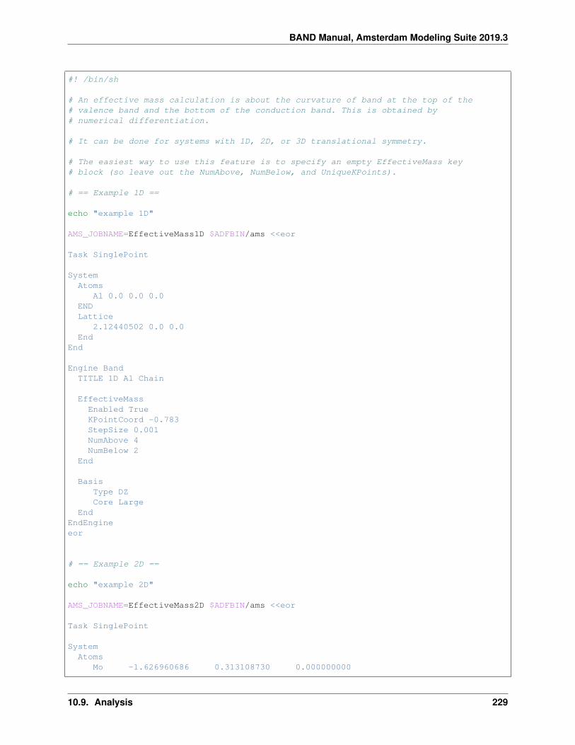
BAND Manual, Amsterdam Modeling Suite 2019.3
#! /bin/sh
# An effective mass calculation is about the curvature of band at the top of the# valence band and the bottom of the conduction band. This is obtained by# numerical differentiation.
# It can be done for systems with 1D, 2D, or 3D translational symmetry.
# The easiest way to use this feature is to specify an empty EffectiveMass key# block (so leave out the NumAbove, NumBelow, and UniqueKPoints).
# == Example 1D ==
echo "example 1D"
AMS_JOBNAME=EffectiveMass1D $ADFBIN/ams <<eor
Task SinglePoint
SystemAtoms
Al 0.0 0.0 0.0ENDLattice
2.12440502 0.0 0.0End
End
Engine BandTITLE 1D Al Chain
EffectiveMassEnabled TrueKPointCoord -0.783StepSize 0.001NumAbove 4NumBelow 2
End
BasisType DZCore Large
EndEndEngineeor
# == Example 2D ==
echo "example 2D"
AMS_JOBNAME=EffectiveMass2D $ADFBIN/ams <<eor
Task SinglePoint
SystemAtoms
Mo -1.626960686 0.313108730 0.000000000
10.9. Analysis 229
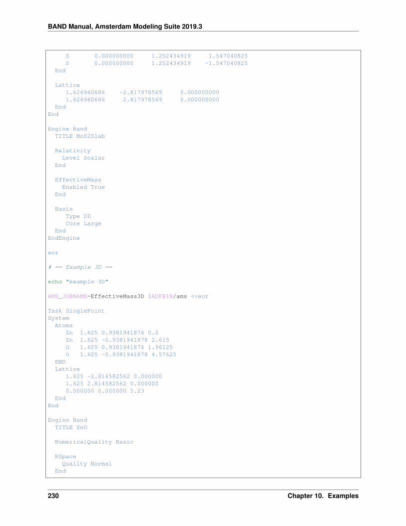
BAND Manual, Amsterdam Modeling Suite 2019.3
S 0.000000000 1.252434919 1.547040825S 0.000000000 1.252434919 -1.547040825
End
Lattice1.626960686 -2.817978569 0.0000000001.626960686 2.817978569 0.000000000
EndEnd
Engine BandTITLE MoS2Slab
RelativityLevel Scalar
End
EffectiveMassEnabled True
End
BasisType DZCore Large
EndEndEngine
eor
# == Example 3D ==
echo "example 3D"
AMS_JOBNAME=EffectiveMass3D $ADFBIN/ams <<eor
Task SinglePointSystem
AtomsZn 1.625 0.9381941876 0.0Zn 1.625 -0.9381941878 2.615O 1.625 0.9381941876 1.96125O 1.625 -0.9381941878 4.57625
ENDLattice
1.625 -2.814582562 0.0000001.625 2.814582562 0.0000000.000000 0.000000 5.23
EndEnd
Engine BandTITLE ZnO
NumericalQuality Basic
KSpaceQuality Normal
End
230 Chapter 10. Examples

BAND Manual, Amsterdam Modeling Suite 2019.3
tails bas=1e-8
EffectiveMassEnabled TrueNumAbove 1NumBelow 1
End
BasisType DZCore Large
EndEndEngine
eor
10.9.10 Example: Generating an Excited State with and Electron Hole
Download Si_ElectronHole.run
#! /bin/sh
# There is the possibility define the excitation of an electron from a low# lying, localized band to a virtual band. The ElectronHole key does allow the# specification of the original band and the spin of the electron. The# EnforcedSpinPolarization key allows to restrict the spin polarization of the# whole system.
$ADFBIN/ams <<eor
Task SinglePoint
SystemAtomsSi.frozen_core -0.67875 -0.67875 -0.67875Si 0.67875 0.67875 0.67875
EndLattice
0.000 2.715 2.7152.715 0.000 2.7152.715 2.715 0.000
EndEnd
Engine Band
TITLE Untitled
BasisType DZPcore noneByAtomType
Si.frozen_core Type=DZP core=LargeEnd
End
10.9. Analysis 231

BAND Manual, Amsterdam Modeling Suite 2019.3
XCLDA SCF VWN
END
UNRESTRICTED
ElectronHoleBandIndex 1SpinIndex 1
End
EnforcedSpinPolarization 0EndEngineeor
10.10 List of Examples
• BasisDefaults (page 152)• BeO_tape41 (page 165)• BetaIron (page 139)• BFieldLdotB (page 140)• BNForce (page 189)• BSSE (page 156)• COChainFreqTS (page 183)• EffectiveMass (page 228)• EField (page 144)• FiniteNucleus (page 146)• Frags_COCu (page 204)• Graphene_Dispersion (page 141)• GraphenePhonons (page 202)• GridKey (page 210)• H2BulkGeo (page 190)• H_ref (page 184)• HonPerovskite_Solvation (page 143)• Li2O_Bader (page 225)• Li_BZPlot (page 227)• Multiresolution_H2O (page 154)• NaCl (page 181)• NEGF (page 167)• NEGF with bias (page 173)• NEGF_Conductance (page 176)• NewResp_3DCopper (page 195)• NewResp_PlotInducedDensity (page 196)• NewResponse for 2D Slab (page 191)• NiO_Hubbard (page 148)• OldResp_Diamond (page 198)• PE-NMR (page 200)• PEDA (page 216)• PEDANOCV (page 219)• Peptide_NumericalQuality (page 152)• PropertiesAtNuclei (page 226)
232 Chapter 10. Examples

BAND Manual, Amsterdam Modeling Suite 2019.3
• Restart a SCF (page 159)• Restart for Properties (page 163)• Si_ElectronHole (page 231)• SnO_EFG (page 201)• TiF3a (page 199)• TiF3g (page 200)• ZnS_ModelPotential (page 149)
10.10. List of Examples 233

BAND Manual, Amsterdam Modeling Suite 2019.3
234 Chapter 10. Examples
CHAPTER
ELEVEN
REQUIRED CITATIONS
When you publish results in the scientific literature which were obtained with programs of the ADF package, you arerequired to include references to the program package with the appropriate release number, and a few key publications.
In addition references to special features are mandatory, in case you have used them.
11.1 General References
For calculations with the periodic structures BAND program, version 2019.3:
1. G. te Velde and E.J. Baerends, Precise density-functional method for periodic structures, Physical Review B 44,7888 (1991) (https://doi.org/10.1103/PhysRevB.44.7888).
2. BAND 2019.3, SCM, Theoretical Chemistry, Vrije Universiteit, Amsterdam, The Netherlands, http://www.scm.com Optionally, you may add the following list of authors and contributors: P.H.T. Philipsen, G. te Velde, E.J.Baerends, J.A. Berger, P.L. de Boeij, M. Franchini, J.A. Groeneveld, E.S. Kadantsev, R. Klooster, F. Kootstra,P. Romaniello, M. Raupach, D.G. Skachkov, J.G. Snijders, C.J.O. Verzijl, J.A. Celis Gil, J. M. Thijssen, G.Wiesenekker, C. A. Peeples, G. Schreckenbach, T. Ziegler.
Note: if you have used a modified (by yourself, for instance) version of the code, you should mention in the citationthat a modified version has been used.
11.2 Feature References
Lead See key references above, for all work with BAND
Suggested G. Wiesenekker, G. te Velde and E.J. Baerends, Analytic quadratic integration over the two-dimensionalBrillouin zone, Journal of Physics C: Solid State Physics 21, 4263 (1988) (https://doi.org/10.1088/0022-3719/21/23/012).
G. Wiesenekker and E.J. Baerends, Quadratic integration over the three-dimensional Brillouin zone, Journal ofPhysics: Condensed Matter 3, 6721 (1991) (https://doi.org/10.1088/0953-8984/3/35/005).
M. Franchini, P.H.T. Philipsen, L. Visscher, The Becke Fuzzy Cells Integration Scheme in the Am-sterdam Density Functional Program Suite, Journal of Computational Chemistry 34, 1818 (2013)(https://doi.org/10.1002/jcc.23323).
M. Franchini, P.H.T. Philipsen, E. van Lenthe, L. Visscher, Accurate Coulomb Potentials for Periodic andMolecular Systems through Density Fitting, Journal of Chemical Theory and Computation 10, 1994 (2014)(https://doi.org/10.1021/ct500172n).
235

BAND Manual, Amsterdam Modeling Suite 2019.3
11.2.1 Geometry optimization
Lead E.S. Kadantsev, R. Klooster. P.L. de Boeij and T. Ziegler, The Formulation and Implementation of AnalyticEnergy Gradients for Periodic Density Functional Calculations with STO/NAO Bloch Basis Set, MolecularPhysics 105, 2583 (2007) (https://doi.org/10.1080/00268970701598063).
11.2.2 TDDFT
Lead F. Kootstra, P.L. de Boeij and J.G. Snijders, Efficient real-space approach to time-dependent density func-tional theory for the dielectric response of nonmetallic crystals, Journal of Chemical Physics 112, 6517 (2000)(https://doi.org/10.1063/1.481315).
P. Romaniello and P.L. de Boeij, Time-dependent current-density-functional theory for the metallic response ofsolids, Physical Review B 71, 155108 (2005) (https://doi.org/10.1103/PhysRevB.71.155108).
Main applications F. Kootstra, P.L. de Boeij, and J.G. Snijders, Application of time-dependent density-functionaltheory to the dielectric function of various nonmetallic crystals, Physical Review B 62, 7071 (2000)(https://doi.org/10.1103/PhysRevB.62.7071).
P. Romaniello, P.L. de Boeij, F. Carbone, and D. van der Marel, Optical properties of bcc transition metals inthe range 0 - 40 eV, Physical Review B 73, 075115 (2006) (https://doi.org/10.1103/PhysRevB.73.075115).
Suggested book references F. Kootstra, Ph.D. thesis (http://www.scm.com/Doc/ft439.pdf), Rijksuniversiteit Gronin-gen, Groningen (2001).
P. Romaniello, Ph.D. thesis (http://www.scm.com/Doc/Thesis_Pina.pdf), Rijksuniversiteit Groningen, Gronin-gen (2006).
A. Berger, Ph.D. thesis (http://www.scm.com/Doc/Thesis_Arjan.pdf), Rijksuniversiteit Groningen, Groningen(2006).
11.2.3 Relativistic TDDFT
Lead P. Romaniello and P.L. de Boeij, Relativistic two-component formulation of time-dependent current-densityfunctional theory: Application to the linear response of solids, Journal of Chemical Physics 127, 174111 (2007)(https://doi.org/10.1063/1.2780146).
11.2.4 Vignale Kohn
Lead J.A. Berger, P.L. de Boeij and R. van Leeuwen, Analysis of the viscoelastic coefficients in the Vignale-Kohnfunctional: The cases of one- and three-dimensional polyacetylene, Physical Review B 71, 155104 (2005)(https://doi.org/10.1103/PhysRevB.71.155104).
Applications J.A. Berger, P. Romaniello, R. van Leeuwen and P.L. de Boeij, Performance of theVignale-Kohn functional in the linear response of metals, Physical Review B 74, 245117 (2006)(https://doi.org/10.1103/PhysRevB.74.245117).
J.A. Berger, P.L. de Boeij, and R. van Leeuwen, Analysis of the Vignale-Kohn current functionalin the calculation of the optical spectra of semiconductors, Physical Review B 75, 35116 (2007)(https://doi.org/10.1103/PhysRevB.75.035116).
236 Chapter 11. Required Citations

BAND Manual, Amsterdam Modeling Suite 2019.3
11.2.5 NMR
Lead D. Skachkov, M. Krykunov, E. Kadantsev, and T. Ziegler, The Calculation of NMR Chemical Shifts in PeriodicSystems Based on Gauge Including Atomic Orbitals and Density Functional Theory, Journal of Chemical Theoryand Computation 6, 1650 (2010) (https://doi.org/10.1021/ct100046a)
D. Skachkov, M. Krykunov, and T. Ziegler, An improved scheme for the calculation of NMR chemical shifts inperiodic systems based on gauge including atomic orbitals and density functional theory, Canadian Journal ofChemistry 89, 1150 (2011) (https://doi.org/10.1139/v11-050).
11.2.6 ESR
A-tensor: Nuclear magnetic dipole hyperfine interaction E.S. Kadantsev and T. Ziegler, Implementation of a Den-sity Functional Theory-Based Method for the Calculation of the Hyperfine A-tensor in Periodic Systems with theUse of Numerical and Slater Type Atomic Orbitals: Application to Paramagnetic Defects, Journal of PhysicalChemistry A 112, 4521 (2008) (https://doi.org/10.1021/jp800494m).
G-tensor: Zeeman interaction E.S. Kadantsev and T. Ziegler, Implementation of a DFT Based Method for the Cal-culation of Zeeman g-tensor in Periodic Systems with the use of Numerical and Slater Type Atomic Orbitals,Journal of Physical Chemistry A 113, 1327 (2009) (https://doi.org/10.1021/jp805466c).
11.2.7 NEGF
Lead
3. (a) O. Verzijl and J. M. Thijssen DFT-Based Molecular Transport Implementation in ADF/BAND, J. Phys.Chem. C, 2012, 116 (46), pp 24393–24412 (https://doi.org/10.1021/jp3044225).
11.3 External programs and Libraries
Click here for the list of programs and/or libraries used in the ADF package. On some platforms optimized librarieshave been used and/or vendor specific MPI implementations.
11.3. External programs and Libraries 237

BAND Manual, Amsterdam Modeling Suite 2019.3
238 Chapter 11. Required Citations

CHAPTER
TWELVE
KEYWORDS
12.1 Links to manual entries
• AIMCriticalPoints (page 93)• ATensor (page 80)• BField (page 37)• BZPath (page 90)• BandStructure (page 89)• Basis (page 42)• BeckeGrid (page 52)• CPVector (page 69)• Convergence (page 62)• DIIS (page 63)• DOS (page 85)• DensityPlot (page 118)• Dependency (page 67)• EFG (page 81)• EField (page 37)• ESR (page 80)• EffectiveMass (page 82)• ElectronHole (page 124)• EnforcedSpinPolarization (page 24)• Fermi (page 69)• FormFactors (page 84)• Fragment (page 94)• FuzzyPotential (page 39)• Grid (page 117)• GridBasedAIM (page 92)• GrossPopulations (page 87)• HubbardU (page 19)• Integration (page 56)• IntegrationMethod (page 55)• KGrpX (page 70)• KSpace (page 49)• LDOS (page 121)• MultiSecantConfig (page 65)• NEGF (page 108)• NMR (page 82)• NOCVOrbitalPlot (page 120)• NOCVdRhoPlot (page 121)• NewResponse (page 73)
239

BAND Manual, Amsterdam Modeling Suite 2019.3
• NewResponseKSpace (page 76)• NewResponseSCF (page 75)• NuclearModel (page 39)• NumericalQuality (page 41)• Occupations (page 124)• OldResponse (page 77)• OrbitalPlot (page 119)• OverlapPopulations (page 88)• PEDA (page 95)• PEDANOCV (page 96)• PeriodicSolvation (page 30)• PotentialNoise (page 124)• RIHartreeFock (page 59)• RadialDefaults (page 55)• Relativity (page 24)• ResponseInducedDensityPlot (page 119)• Restart (page 115)• SCF (page 60)• Save (page 122)• Screening (page 67)• SoftConfinement (page 46)• Solvation (page 27)• SolvationSM12 (page 31)• StoreHamiltonian2 (page 113)• SubSymmetry (page 123)• Tails (page 66)• Unrestricted (page 24)• UseSymmetry (page 123)• ZlmFit (page 56)
12.2 Summary of all keywords
AIMCriticalPoints
Type Block
Description Compute the critical points of the density (Atoms In Molecules). The algorithm startsfrom a regular mesh of points, and from each of these it walks towards its corresponding criticalpoint.
Enabled
Type Bool
Default value False
GUI name : Critical points and bond paths
Description Compute the critical points of the density (Atoms In Molecules). The algorithmstarts from a regular mesh of points, and from each of these it walks towards its correspondingcritical point.
EqvPointsTol
Type Float
Default value 0.27
240 Chapter 12. Keywords

BAND Manual, Amsterdam Modeling Suite 2019.3
Unit Bohr
Description If the distance between two critical points is smaller than this value, the two criticalpoints are considered to be the same point.
GridPadding
Type Float
Default value 0.7
Unit Bohr
Description How much extra space is added to the starting guess domain in the search for thecritical points
GridSpacing
Type Float
Default value 0.5
Unit Bohr
Description The distance between the initial trial points.
Allow
Type String
Recurring True
Description Debugging feature to let the program continue even when intermediate results seem tobe wrong or very inaccurate
ATensor
Type Block
Description Hyperfine A-tensor.
Enabled
Type Bool
Default value False
GUI name :A-tensor
Description Compute the hyperfine A-tensor. Note: Unrestricted calculation is required.
AtomType
Type Block
Recurring True
Description Explicit basis set definition for given atom type.
AutomaticGaussians
Type Non-standard block
Description Definition of the automatic gaussians
BasisFunctions
Type Non-standard block
Description Definition of the extra Slater-type orbitals
12.2. Summary of all keywords 241

BAND Manual, Amsterdam Modeling Suite 2019.3
Dirac
Type Non-standard block
Description Specification of the numerical (‘Herman-Skillman’) free atom, which defines theinitial guess for the SCF density, and which also (optionally) supplies Numerical AtomicOrbitals (NOs) as basis functions
FitFunctions
Type Non-standard block
Description Slater-type fit functions. Obsolete feature.
BandStructure
Type Block
Description Options for the calculation of the band structure.
Automatic
Type Bool
Default value True
GUI name Automatic generate path
Description If True, BAND will automatically generate the standard path through the Brillouinzone. If False BAND will use the user-defined path in BZPath.
DeltaK
Type Float
Default value 0.1
Unit 1/Bohr
GUI name Interpolation delta-K
Description Step (in reciprocal space) for band structure interpolation. Using a smaller number(e.g. 0.03) will result in smoother band curves at the cost of an increased computation time.
Enabled
Type Bool
Default value False
GUI name Calculate band structure
Description If True, Band will calculate the band structure and save it to file for visualization.
EnergyAboveFermi
Type Float
Default value 0.75
Unit Hartree
GUI name Energy above Fermi level
Description Bands with minimum energy larger then FermiEnergy + EnergyAboveFermi arenot saved to file. Increasing the value of EnergyAboveFermi will result in more unoccupiedbands to be saved to file for visualization.
EnergyBelowFermi
242 Chapter 12. Keywords

BAND Manual, Amsterdam Modeling Suite 2019.3
Type Float
Default value 10.0
Unit Hartree
GUI name Energy below Fermi level
Description Bands with maximum energy smaller then FermiEnergy - EnergyBelowFermi arenot saved to file. Increasing the value of EnergyBelowFermi will result in more occupiedcore bands to be saved to file for visualization. Note: EnergyBelowFermi should be a positivenumber!
FatBands
Type Bool
Default value True
GUI name Calculate fatbands
Description If True, BAND will compute the fat bands (only if BandStructure%Enabled isTrue). The Fat Bands are the periodic equivalent of the Mulliken population analysis.
UseSymmetry
Type Bool
Default value True
GUI name Use symmetry
Description If True, only the irreducible wedge of the Wigner-Seitz cell is sampled. If False,the whole (inversion-unique) Wigner-Seitz cell is sampled. Note: The Symmetry key doesnot influence the symmetry of the band structure sampling.
Basis
Type Block
Description Definition of the basis set
ByAtomType
Type Non-standard block
Description Definition of the basis set for specific atom types (one definition per line). Format:‘AtomType Type=Type Core=Core’. Example: ‘C.large_basis Type=TZ2P Core=None’
Core
Type Multiple Choice
Default value Large
Options [None, Small, Medium, Large]
Description Size of the frozen core.
Folder
Type String
Description Path to a folder containing the basis set files. This can be used for special use-defined basis sets. Cannot be used in combination with ‘Type’
Type
Type Multiple Choice
12.2. Summary of all keywords 243

BAND Manual, Amsterdam Modeling Suite 2019.3
Default value DZ
Options [SZ, DZ, DZP, TZP, TZ2P, QZ4P]
Description The basis sets to be used.
BeckeGrid
Type Block
Description Options for the numerical integration grid, which is a refined version of the fuzzy cellsintegration scheme developed by Becke.
AtomDepQuality
Type Non-standard block
Description One can define a different grid quality for each atom (one definition per line). Lineformat: ‘AtomIndex Quality’, e.g. ‘3 Good’ means that a grid of Good quality will be usedfor the third atom in input order. If the index of an atom is not present in the AtomDepQualitysection, the quality defined in the Quality key will be used
Quality
Type Multiple Choice
Default value Auto
Options [Auto, Basic, Normal, Good, VeryGood, Excellent]
Description Quality of the integration grid. For a description of the various qualities and theassociated numerical accuracy see reference. If ‘Auto’, the quality defined in the ‘Numeri-calQuality’ will be used.
RadialGridBoost
Type Float
Default value 1.0
Description The number of radial grid points will be boosted by this factor. Some XC func-tionals require very accurate radial integration grids, so BAND will automatically boost theradial grid by a factor 3 for the following numerically sensitive functionals: LibXC M05,LibXC M05-2X, LibXC M06-2X, LibXC M06-HF, LibXC M06-L, LibXC M08-HX, LibXCM08-SO, LibXC M11-L, LibXC MS0, LibXC MS1, LibXC MS2, LibXC MS2H, LibXCMVS, LibXC MVSH, LibXC N12, LibXC N12-SX, LibXC SOGGA11, LibXC SOGGA11-X, LibXC TH1, LibXC TH2, LibXC WB97, LibXC WB97X, MetaGGA M06L, MetaHybridM06-2X, MetaHybrid M06-HF, MetaGGA MVS.
BField
Type Block
Description The effect of a magnetic filed can be approximated by the following potential: mu* sigma_i * B, where mu is the Bohr magneton, sigma_i are the Pauli matrices and B is themagnetic field
Bx
Type Float
Default value 0.0
Unit Tesla
Description Value of the x component of the BField
244 Chapter 12. Keywords

BAND Manual, Amsterdam Modeling Suite 2019.3
By
Type Float
Default value 0.0
Unit Tesla
Description Value of the y component of the BField
Bz
Type Float
Default value 0.0
Unit Tesla
Description Value of the z component of the BField
Dipole
Type Bool
Default value False
GUI name Bfield is: Atomic dipole
Description Use an atomic dipole as magnetic field instead of a uniform magnetic field.
DipoleAtom
Type Integer
Default value 1
GUI name on atom number
Description Atom on which the magnetic dipole should be centered (if using the dipole option)
Method
Type Multiple Choice
Default value NR_SDOTB
Options [NR_SDOTB, NR_LDOTB, NR_SDOTB_LDOTB]
Description There are two terms coupling to an external magnetic field. One is the intrinsic spinof the electron, called S-dot-B, the other one is the orbital momentum call L-dot-B. The L.Bis implemented non-relativistically, using GIAOs in the case of a homogeneous magneticfield (not for the dipole case).
Unit
Type Multiple Choice
Default value tesla
Options [tesla, a.u.]
Description Unit of magnetic filed. The a.u. is the SI version of a.u.
BZPath
Type Block
Description Definition of the user-defined path in the Brillouin zone for band structure plotting.
path
12.2. Summary of all keywords 245
BAND Manual, Amsterdam Modeling Suite 2019.3
Type Non-standard block
Recurring True
Description Definition of the k-points in a path. The vertices of your path should be defined infractional coordinates (wrt the reciprocal lattice vectors)
Comment
Type Non-standard block
Description The content of this block will be copied to the output header as a comment to thecalculation.
Convergence
Type Block
Description Options and parameters related to the convergence behavior of the SCF procedure.
Criterion
Type Float
Description Criterion for termination of the SCF procedure. The default depends on the Numer-icalQuality and on the number of atoms in the system.
Degenerate
Type String
Default value default
Description Smooths (slightly) occupation numbers around the Fermi level, so as to insure thatnearly-degenerate states get (nearly-) identical occupations. Be aware: In case of problematicSCF convergence the program will turn this key on automatically, unless the key ‘Nodegen-erate’ is set in input. The smoothing depends on the argument to this key, which can beconsidered a ‘degeneration width’. When the argument reads default, the program will usethe value 1e-4 a.u. for the energy width.
ElectronicTemperature
Type Float
Default value 0.0
Unit a.u.
Description Simulates a finite-temperature electronic distribution using the defined energy. Thismay be used to achieve convergence in an otherwise problematically converging system.The energy of a finite-T distribution is different from the T=0 value, but for small T a fairapproximation of the zero-T energy is obtained by extrapolation. The extrapolation energycorrection term is printed with the survey of the bonding energy in the output file. Check thatthis value is not too large. Build experience yourself how different settings may affect theoutcomes. Note: this key is meant to help you overcome convergence problems, not to dofinite-temperature research! Only the electronic distribution is computed T-dependent, otheraspects are not accounted for!
InitialDensity
Type Multiple Choice
Default value rho
Options [rho, psi]
246 Chapter 12. Keywords

BAND Manual, Amsterdam Modeling Suite 2019.3
Description The SCF is started with a guess of the density. There are the following choicesRHO: the sum of atomic density. PSI: construct an initial eigensystem by occupying theatomic orbitals. The guessed eigensystem is orthonormalized, and from this the density iscalculated/
LessDegenerate
Type Bool
Default value False
Description If smoothing of occupations over nearly degenerate orbitals is applied (see Degen-erate key), then, if this key is set in the input file, the program will limit the smoothing energyrange to 1e-4 a.u. as soon as the SCF has converged ‘halfway’, i.e. when the SCF error hasdecreased to the square root of its convergence criterion.
NoDegenerate
Type Bool
Default value False
Description This key prevents any internal automatic setting of the key DEGENERATE.
SpinFlip
Type Integer List
GUI name Flip spin for atoms
Description List here the atoms for which you want the initial spin polarization to be flipped.This way you can distinguish between ferromagnetic and anti ferromagnetic states. Cur-rently, it is not allowed to give symmetry equivalent atoms a different spin orientation. Toachieve that you have to break the symmetry.
startwithmaxspin
Type Bool
Default value True
Description To break the initial perfect symmetry of up and down densities there are two strate-gies. One is to occupy the numerical orbitals in a maximum spin configuration. The alterna-tive is to add a constant to the potential. See also Vsplit key.
CPVector
Type Integer
Default value 128
GUI name Vectorlength (blocksize)
Description The code is vectorized and this key can be used to set the vector length
DensityPlot
Type Non-standard block
Description Plots of the density. Goes together with the Restart%DensityPlot and Grid keys.
Dependency
Type Block
Description Criteria for linear dependency of the basis and fit set
Basis
12.2. Summary of all keywords 247

BAND Manual, Amsterdam Modeling Suite 2019.3
Type Float
Default value 1e-08
GUI name Dependency criterion
Description Criteria for linear dependency of the basis: smallest eigenvalue of the overlap ma-trix of normalized Bloch functions.
Core
Type Float
Default value 0.98
Description The program verifies that the frozen core approximation is reasonable, by checkingthe smallest value of the overlap matrix of the core (Bloch) orbitals against this criterion.
CoreValence
Type Float
Default value 1e-05
Description Criterion for dependency of the core functions on the valence basis. The maximumoverlap between any two normalized functions in the two respective function spaces shouldnot exceed 1.0-corevalence
Fit
Type Float
Default value 5e-06
Description Criterion for dependency of the total set of fit functions. The value monitored isthe smallest eigenvalue of the overlap matrix of normalized Bloch sums of symmetrized fitfunctions.
DIIS
Type Block
Description Parameters for the DIIS procedure to obtain the SCF solution
Adaptable
Type Bool
Default value True
Description Change automatically the value of dimix during the SCF.
CHuge
Type Float
Default value 20.0
GUI name No DIIS (but damping) when coefs >
Description When the largest coefficient in the DIIS expansion exceeds this value, damping isapplied
CLarge
Type Float
Default value 20.0
248 Chapter 12. Keywords

BAND Manual, Amsterdam Modeling Suite 2019.3
GUI name Reduce DIIS space when coefs >
Description When the largest DIIS coefficient exceeds this value, the oldest DIIS vector is re-moved and the procedure re-applied
Condition
Type Float
Default value 1000000.0
Description The condition number of the DIIS matrix, the largest eigenvalue divided by thesmallest, must not exceed this value. If this value is exceeded, this vector will be removed.
DiMix
Type Float
Default value 0.2
GUI name Bias DIIS towards latest vector with
Description Mixing parameter for the DIIS procedure
NCycleDamp
Type Integer
Default value 1
GUI name Do not start DIIS before cycle
Description Number of initial iterations where damping is applied, before any DIIS is consid-ered
NVctrx
Type Integer
Default value 20
GUI name Size of DIIS space
Description Maximum number of DIIS expansion vectors
Variant
Type Multiple Choice
Default value DIIS
Options [DIIS, LISTi, LISTb, LISTd]
Description Which variant to use. In case of problematic SCF convergence, first try MultiSe-cant, and if that does not work the LISTi is the advised method. Note: LIST is computation-ally more expensive per SCF iteration than DIIS.
DOS
Type Block
Description Density-Of-States (DOS) options
CalcPopulationAnalysis
Type Bool
Default value True
GUI name Calculate DOS
12.2. Summary of all keywords 249

BAND Manual, Amsterdam Modeling Suite 2019.3
Description Whether or not to calculate the population analysis. If the DOS%Enabled is true,this will also be true. Population analysis can become very expensive when there are manysymmetry operators, such as in a super cell.
DeltaE
Type Float
Default value 0.005
Unit Hartree
Description Energy step for the DOS grid. Using a smaller value (e.g. half the default value)will result in a finer sampling of the DOS.
Enabled
Type Bool
Default value False
GUI name Calculate DOS
Description Whether or not to calculate the density of states.
Energies
Type Integer
Description Number of equidistant energy-values for the DOS grid. This keyword supersedesthe ‘DeltaE’ keyword.
File
Type String
Description Write the DOS (plain text format) to the specified file instead of writing it to thestandard output.
IntegrateDeltaE
Type Bool
Default value True
Description This subkey handles which algorithm is used to calculate the data-points in theplotted DOS. If true, the data-points represent an integral over the states in an energy interval.Here, the energy interval depends on the number of Energies and the user-defined upper andlower energy for the calculation of the DOS. The result has as unit [number of states / (energyinterval * unit cell)]. If false, the data-points do represent the number of states for a specificenergy and the resulting plot is equal to the DOS per unit cell (unit: [1/energy]). Since theresulting plot can be a wild function and one might miss features of the DOS due to the steplength between the energies, the default is set to the integration algorithm.
Max
Type Float
Unit Hartree
Description User defined upper bound energy (with respect to the Fermi energy)
Min
Type Float
Unit Hartree
250 Chapter 12. Keywords
BAND Manual, Amsterdam Modeling Suite 2019.3
Description User defined lower bound energy (with respect to the Fermi energy)
StoreCoopPerBasPair
Type Bool
Default value False
GUI name Calculate: COOP
Description Calculate the COOP (crystal orbital overlap population).
DosBas
Type Non-standard block
Description Used to specify the fragment basis for the DOS.
EffectiveMass
Type Block
Description In a semi-conductor, the mobility of electrons and holes is related to the curvature of thebands at the top of the valence band and the bottom of the conduction band. With the effectivemass option, this curvature is obtained by numerical differentiation. The estimation is done withthe specified step size, and twice the specified step size, and both results are printed to give ahint on the accuracy. The easiest way to use this key is to enabled it without specifying any extraoptions.
Enabled
Type Bool
Default value False
GUI name Effective mass
Description Compute the EffectiveMass.
KPointCoord
Type Float List
Unit 1/Bohr
Recurring True
Description Coordinate of the k-points for which you would like to compute the effective mass.
NumAbove
Type Integer
Default value 1
Description Number of bands to take into account above the Fermi level.
NumBelow
Type Integer
Default value 1
Description Number of bands to take into account below the Fermi level.
StepSize
Type Float
Default value 0.001
12.2. Summary of all keywords 251

BAND Manual, Amsterdam Modeling Suite 2019.3
Description Size of the step taken in reciprocal space to perform the numerical differentiation
EFG
Type Block
Description The electronic charge density causes an electric field, and the gradient of this field cou-ples with the nuclear quadrupole moment, that some (non-spherical) nuclei have and can bemeasured by several spectroscopic techniques. The EFG tensor is the second derivative of theCoulomb potential at the nuclei. For each atom it is a 3x3 symmetric and traceless matrix. Diag-onalization of this matrix gives three eigenvalues, which are usually ordered by their decreasingabsolute size and denoted as V_xx, V_yy, V_zz. The result is summarized by the largesteigenvalue and the asymmetry parameter.
Enabled
Type Bool
Default value False
GUI name EFG (electric field gradient): Calculate
Description Compute the EFG tensor (for nuclear quadrupole interaction).
EField
Type Block
Description Include a homogeneous, static, electric field in the z-direction (only possible for 0D,1D or 2D periodic systems)
Ez
Type Float
Default value 0.0
GUI name Electric field - Z
Description Strength of the electric field, in units as selected with the EField unit key.
unit
Type Multiple Choice
Default value Volt/Angstrom
Options [Volt/Angstrom, a.u., Volt/Bohr, Volt/meter]
Description Unit of the electric field Ez
EigThreshold
Type Float
Default value 0.01
Description Threshold for printing the eigenvectors coefficients (Print Eigens)
ElectronHole
Type Block
Description Allows one to specify an occupied band which shall be depopulated, where the elec-trons are then moved to the Fermi level. For a spin-restricted calculation 2 electrons are shiftedand for a spin-unrestricted calculation only one electron is shifted.
BandIndex
252 Chapter 12. Keywords

BAND Manual, Amsterdam Modeling Suite 2019.3
Type Integer
Description Which occupied band shall be depopulated.
SpinIndex
Type Integer
Description Defines the spin of the shifted electron (1 or 2).
EmbeddingPotential
Type Block
Description An external potential can be read in and will be added to the effective Kohn-Shampotential. It has to be on the becke grid
Filename
Type String
Default value
Description Name of the file containing the embedding potential.
PotentialName
Type String
Default value
Description Name of variable containing the potential.
EnforcedSpinPolarization
Type Float
GUI name Spin polarization
Description Enforce a specific spin-polarization instead of occupying according to the aufbau prin-ciple. The spin-polarization is the difference between the number of alpha and beta electron.Thus, a value of 1 means that there is one more alpha electron than beta electrons. The numbermay be anything, including zero, which may be of interest when searching for a spin-flippedpair, that may otherwise end up in the (more stable) parallel solution.
ESR
Type Block
Description Zeeman g-tensor. The Zeeman g-tensor is implemented using two-component approachof Van Lenthe and co-workers in which the g-tensor is computed from a pair of spinors relatedto each other by time-reversal symmetry. Note: the following options are necessary for ESR:‘Relativistic zora spin’ and ‘Kspace 1’
Enabled
Type Bool
Default value False
GUI name ESR: g-tensor
Description Compute Zeeman g-tensor. The Zeeman g-tensor is implemented using two-component approach of Van Lenthe and co-workers in which the g-tensor is computed from apair of spinors related to each other by time-reversal symmetry. Note: the following optionsare necessary for ESR: ‘Relativistic zora spin’ and ‘Kspace 1’
Fermi
12.2. Summary of all keywords 253
BAND Manual, Amsterdam Modeling Suite 2019.3
Type Block
Description Technical parameter used in determining the Fermi energy, which is carried out at eachcycle of the SCF procedure.
Delta
Type Float
Default value 0.0001
Description Convergence criterion: upper and lower bounds for the Fermi energy and the cor-responding integrated charge volumes must be equal within delta.
Eps
Type Float
Default value 1e-10
Description After convergence of the Fermi energy search procedure, a final estimate is definedby interpolation and the corresponding integrated charge volume is tested. It should be exact,to machine precision. Tested is that it deviates not more than eps.
MaxTry
Type Integer
Default value 15
Description Maximum number of attempts to locate the Fermi energy. The procedure is itera-tive in nature, narrowing the energy band in which the Fermi energy must lie, between anupper and a lower bound. If the procedure has not converged sufficiently within MaxTryiterations, the program takes a reasonable value and constructs the charge density by interpo-lation between the functions corresponding to the last used upper and lower bounds for theFermi energy.
FormFactors
Type Integer
Default value 2
Description Number of stars of K-vectors for which the form factors are computed
Fragment
Type Block
Recurring True
Description Defines a fragment. You can define several fragments for a calculation.
AtomMapping
Type Non-standard block
Description Format ‘indexFragAt indexCurrentAt’. One has to associate the atoms of the frag-ment to the atoms of the current calculation. So, for each atom of the fragment the indexFra-gAt has to be associated uniquely to the indexCurrentAt for the current calculation.
Filename
Type String
Description Filename of the fragment. Absolute path or path relative to the executing directory.
Labels
254 Chapter 12. Keywords
BAND Manual, Amsterdam Modeling Suite 2019.3
Type Non-standard block
Description This gives the possibility to introduce labels for the fragment orbitals. See exam-ples.
FuzzyPotential
Type Non-standard block
Description Atomic (fuzzy cell) based, external, electric potential. See example.
Grid
Type Block
Description Options for the regular grid used for plotting (e.g. density plot). Used ICW the restartoption.
ExtendX
Type Float
Default value 0.0
Unit Bohr
Description Extend the default regular grid along the x-direction by the specified amount:[x_min, x_max] => [x_min - ExtendX/2, x_max + ExtendX/2].
ExtendY
Type Float
Default value 0.0
Unit Bohr
Description Extend the default regular grid along the y-direction by the specified amount:[y_min, y_max] => [y_min - ExtendY/2, y_max + ExtendY/2].
ExtendZ
Type Float
Default value 0.0
Unit Bohr
Description Extend the default regular grid along the z-direction by the specified amount:[z_min, z_max] => [z_min - ExtendZ/2, z_max + ExtendZ/2].
FileName
Type String
Default value
Description Read in the grid from a file. The file format of the grid is: three numbers per line(defining the x, y and z coordinates of the points).
Type
Type Multiple Choice
Default value coarse
Options [coarse, medium, fine]
Description The default regular grids.
12.2. Summary of all keywords 255
BAND Manual, Amsterdam Modeling Suite 2019.3
UserDefined
Type Non-standard block
Description Once can define the regular grid specification in this block. See example.
GridBasedAIM
Type Block
Description Invoke the ultra fast grid based Bader analysis.
Enabled
Type Bool
Default value False
GUI name Bader (AIM): Atomic properties
Description Invoke the ultra fast grid based Bader analysis.
Iterations
Type Integer
Default value 40
Description The maximum number of steps that may be taken to find the nuclear attractor for agrid point.
SmallDensity
Type Float
Default value 1e-06
Description Value below which the density is ignored. This should not be chosen too smallbecause it may lead to unassignable grid points.
UseStartDensity
Type Bool
Default value False
Description Whether the analysis is performed on the startup density (True) or on the finaldensity (False).
GrossPopulations
Type Non-standard block
Description Partial DOS (pDOS) are generated for the gross populations listed under this key. Seeexample.
HubbardU
Type Block
Description Options for Hubbard-corrected DFT calculations.
Enabled
Type Bool
Default value False
Description Whether or not to apply the Hubbard Hamiltonian
256 Chapter 12. Keywords
BAND Manual, Amsterdam Modeling Suite 2019.3
LValue
Type String
Default value
Description For each atom type specify the l value (0 - s orbitals, 1 - p orbitals, 2 - d orbitals).A negative value is interpreted as no l-value.
PrintOccupations
Type Bool
Default value True
Description Whether or not to print the occupations during the SCF.
UValue
Type String
Default value
Description For each atom type specify the U value (in atomic units). A value of 0.0 is inter-preted as no U.
Integration
Type Block
Description Options for the Voronoi numerical integration scheme. Deprecated. Use BeckeGridinstead.
AccInt
Type Float
Default value 3.5
Description General parameter controlling the accuracy of the Voronoi integration grid. A valueof 3 would be basic quality and a value of 7 would be good quality.
IntegrationMethod
Type Multiple Choice
Default value Becke
Options [Becke, Voronoi]
Description Choose the real-space numerical integration method. Note: the Voronoi integrationscheme is deprecated.
KGrpX
Type Integer
Default value 5
GUI name Number of K-points at once
Description Absolute upper bound on the number of k-points processed together. This only affectsthe computational performance.
KSpace
Type Block
Description Options for the k-space integration (i.e. the grid used to sample the Brillouin zone)
12.2. Summary of all keywords 257

BAND Manual, Amsterdam Modeling Suite 2019.3
Quality
Type Multiple Choice
Default value Auto
Options [Auto, GammaOnly, Basic, Normal, Good, VeryGood, Excellent]
GUI name K-space
Description Select the quality of the K-space grid used to sample the Brillouin Zone. If ‘Auto’,the quality defined in the ‘NumericalQuality’ will be used. If ‘GammaOnly’, only one point(the gamma point) will be used. The actual number of K points generated depends on thisoption and on the size of the unit cell. The larger the real space cell, the fewer K points willbe generated. The CPU-time and accuracy strongly depend on this option.
Regular
Type Block
Description Options for the regular k-space integration grid.
NumberOfPoints
Type Integer List
Description Use a regular grid with the specified number of k-points along each recipro-cal lattice vector. For 1D periodic systems you should specify only one number, for 2Dsystems two numbers, and for 3D systems three numbers.
Symmetric
Type Block
Description Options for the symmetric k-space integration grid.
KInteg
Type Integer
GUI name Accuracy
Description Specify the accuracy for the Symmetric method. 1: absolutely minimal (onlythe G-point is used) 2: linear tetrahedron method, coarsest spacing 3: quadratic tetrahedronmethod, coarsest spacing 4,6,... (even): linear tetrahedron method 5,7.... (odd): quadraticmethod The tetrahedron method is usually by far inferior.
Type
Type Multiple Choice
Default value Regular
Options [Regular, Symmetric]
GUI name K-space grid type
Description The type of k-space integration grid used to sample the Brillouin zone (BZ) used.‘Regular’: simple regular grid. ‘Symmetric’: symmetric grid for the irreducible wedge ofthe first BZ (useful when high-symmetry points in the BZ are needed to capture the correctphysics of the system, graphene being a notable example).
LDOS
Type Block
258 Chapter 12. Keywords

BAND Manual, Amsterdam Modeling Suite 2019.3
Description Local Density-Of-States information. This can be used to generate STM images in theTersoff-Hamann approximation (see https://doi.org/10.1103/PhysRevB.31.805)
DeltaNeg
Type Float
Default value 0.0001
Unit Hartree
Description Lower bound energy (Shift-DeltaNeg)
DeltaPos
Type Float
Default value 0.0001
Unit Hartree
Description Upper bound energy (Shift+DeltaPos)
Shift
Type Float
Default value 0.0
Unit Hartree
Description The energy bias with respect to the Fermi level.
MolecularNMR
Type Block
Description Options for the calculations of the NMR shielding tensor for molecules, excluding pe-riodic systems. Implements the Schreckenbach method like ADF.
Enabled
Type Bool
Default value False
Description Compute NMR shielding.
MultiSecantConfig
Type Block
Description Parameters for the Multi-secant SCF convergence method.
CMax
Type Float
Default value 20.0
GUI name Max coeff
Description Maximum coefficient allowed in expansion
InitialSigmaN
Type Float
Default value 0.1
GUI name Initial
12.2. Summary of all keywords 259

BAND Manual, Amsterdam Modeling Suite 2019.3
Description This is a lot like a mix factor: bigger means bolder
MaxSigmaN
Type Float
Default value 0.3
GUI name Max
Description Upper bound for the SigmaN parameter
MaxVectors
Type Integer
Default value 20
GUI name Number of cycles to use
Description Maximum number of previous cycles to be used
MinSigmaN
Type Float
Default value 0.01
GUI name Min
Description Lower bound for the SigmaN parameter
NEGF
Type Block
Description Options for the NEGF (non-equilibrium green function) transport calculation.
AlignChargeTol
Type Float
Default value 0.1
Description In an alignment run you want to get the number of electrons in the center right. Thisnumber specifies the criterion for that.
AlignmentFile
Type String
Default value
Description Band result file (.rkf) corresponding to the alignment calculation.
Alpha
Type Float
Default value 1e-05
Description A charge error needs to be translated in a potential shift. DeltaV = alpha * DeltaQ
ApplyShift1
Type Bool
Default value True
Description Apply the main shift, obtained from comparing matrix elements in the leads withthose from the tight-binding run. Strongly recommended.
260 Chapter 12. Keywords

BAND Manual, Amsterdam Modeling Suite 2019.3
ApplyShift2
Type Bool
Default value True
Description Apply the smaller alignment shift. This requires an extra alignment run. Usuallythis shift is smaller.
AutoContour
Type Bool
Default value True
Description Use automatic contour integral.
BiasPotential
Type Float
Default value 0.0
Description Apply a bias potential (atomic units). Can be negative. One has to specify the ramppotential with the FuzzyPotential key. This is mostly conveniently done with the GUI.
BoundOccupationMethod
Type Integer
Default value 1
Description See text. Only relevant with NonEqDensityMethod equal 2 or 3.
CDIIS
Type Bool
Default value False
Description Make the normal DIIS procedure aware of the align charge error
CheckOverlapTol
Type Float
Default value 0.01
Description BAND checks how well the TB overlap matrix S(R=0) represents the overlap ma-trix in the lead region. Elements corresponding to the outer layer are neglected, becausewhen using a frozen core they have bigger errors.
ContourQuality
Type Multiple Choice
Default value good
Options [basic, normal, good, verygood]
Description The density matrix is calculated numerically via a contour integral. Changing thequality influences the number of points. This influences a lot the performance.
DEContourInt
Type Float
Default value -1.0
Description The energy interval for the contour grid. Defaults depends on the contour quality
12.2. Summary of all keywords 261

BAND Manual, Amsterdam Modeling Suite 2019.3
DERealAxisInt
Type Float
Default value -1.0
Description The energy interval for the real axis grid. Defaults depends on the contour quality.
DeltaPhi0
Type Float
Default value 0.0
Description Undocumented.
DeltaPhi1
Type Float
Default value 0.0
Description Undocumented.
DoAlignment
Type Bool
Default value False
Description Set this to True if you want to do an align run. Between the leads there should belead material. The GUI can be of help here.
EMax
Type Float
Default value 5.0
Unit eV
Description The maximum energy for the transmission grid (with respect to the Fermi level ofthe lead)
EMin
Type Float
Default value -5.0
Unit eV
Description The minimum energy for the transmission grid (with respect to the Fermi level ofthe lead)
Eta
Type Float
Default value 1e-05
Description Small value used for the contour integral: stay at least this much above the real axis.This value is also used for the evaluation of the Transmission and dos.
IgnoreOuterLayer
Type Bool
Default value True
262 Chapter 12. Keywords

BAND Manual, Amsterdam Modeling Suite 2019.3
Description Whether or not to ignore the outer layer.
KT
Type Float
Default value 0.001
Description k-Boltzman times temperature.
LeadFile
Type String
Default value
Description File containing the tight binding representation of the lead.
NE
Type Integer
Default value 100
Description The number of energies for the transmission energy grid.
NonEqDensityMethod
Type Integer
Default value 1
Description See text.
SGFFile
Type String
Default value
Description The result from the SGF program. Contains the Fermi energy of the lead.
YContourInt
Type Float
Default value 0.3
Description The density is calculated via a contour integral. This value specifies how far abovethe real axis the (horizontal part of the) contour runs. The value is rounded in such a waythat it goes exactly halfway between two Fermi poles. There is a trade off: making it biggermakes the integrand more smooth, but the number of enclosed poles increases. For lowtemperatures it makes sense to lower this value, and use a smaller deContourInt.
YRealaxisInt
Type Float
Default value 1e-05
Description The non-Equilibrium density is calculated near the real axis.
NewResponse
Type Block
Description The TD-CDFT calculation to obtain the dielectric function is computed when this blockis present in the input. Several important settings can be defined here.
ActiveESpace
12.2. Summary of all keywords 263

BAND Manual, Amsterdam Modeling Suite 2019.3
Type Float
Default value 5.0
Unit eV
GUI name Active energy space
Description Modifies the energy threshold (DeltaE^max_thresh = omega_high + Ac-tiveESpace) for which single orbital transitions (DeltaEpsilon_ia = Epsilon_a^virtual- Epsilon_i^occupied) are taken into account.
ActiveXYZ
Type String
Default value t
Description Expects a string consisting of three letters of either ‘T’ (for true) or ‘F’ (for false)where the first is for the X-, the second for the Y- and the third for the Z-component of theresponse properties. If true, then the response properties for this component will be evaluated.
DensityCutOff
Type Float
Default value 0.001
GUI name Volume cutoff
Description For 1D and 2D systems the unit cell volume is undefined. Here, the volume iscalculated as the volume bordered by the isosurface for the value DensityCutoff of the totaldensity.
EShift
Type Float
Default value 0.0
Unit eV
GUI name Shift
Description Energy shift of the virtual crystal orbitals.
FreqHigh
Type Float
Default value 3.0
Unit eV
Description Upper limit of the frequency range for which response properties are calculated(omega_high).
FreqLow
Type Float
Default value 1.0
Unit eV
Description Lower limit of the frequency range for which response properties are calculated.(omega_low)
NFreq
264 Chapter 12. Keywords
BAND Manual, Amsterdam Modeling Suite 2019.3
Type Integer
Default value 5
Description Number of frequencies for which a linear response TD-CDFT calculation is per-formed.
NewResponseKSpace
Type Block
Description Modify the details for the integration weights evaluation in reciprocal space for eachsingle-particle transition. Only influencing the NewResponse code.
Eta
Type Float
Default value 1e-05
Description Defines the small, finite imaginary number i*eta which is necessary in the contextof integration weights for single-particle transitions in reciprocal space.
SubSimp
Type Integer
Default value 3
Description determines into how many sub-integrals each integration around a k point is split.This is only true for so-called quadratic integration grids. The larger the number the betterthe convergence behavior for the sampling in reciprocal space. Note: the computing time forthe weights is linear for 1D, quadratic for 2D and cubic for 3D!
NewResponseSCF
Type Block
Description Details for the linear-response self-consistent optimization cycle. Only influencing theNewResponse code.
Bootstrap
Type Integer
Default value 0
Description defines if the Berger2015 kernel (Bootstrap 1) is used or not (Bootstrap 0). If youchose the Berger2015 kernel, you have to set NewResponseSCF%XC to ‘0’. Since it shall beused in combination with the bare Coulomb response only. Note: The evaluation of responseproperties using the Berger2015 is recommend for 3D systems only!
COApproach
Type Bool
Default value True
Description The program automatically decides to calculate the integrals and induced densi-ties via the Bloch expanded atomic orbitals (AO approach) or via the cyrstal orbitals (COapproach). The option COApproach overrules this decision.
COApproachBoost
Type Bool
Default value False
12.2. Summary of all keywords 265

BAND Manual, Amsterdam Modeling Suite 2019.3
GUI name CO Approach Boost
Description Keeps the grid data of the Crystal Orbitals in memory. Requires significantly morememory for a speedup of the calculation. One might have to use multiple computing nodesto not run into memory problems.
Criterion
Type Float
Default value 0.001
Description For the SCF convergence the RMS of the induced density change is tested. If thisvalue is below the Criterion the SCF is finished. Furthermore, one can find the calculatedelectric susceptibility for each SCF step in the output and can therefore decide if the defaultvalue is too loose or too strict.
DIIS
Type Bool
Default value True
Description In case the DIIS method is not working, one can switch to plain mixing by settingDIIS to false.
LowFreqAlgo
Type Bool
Default value True
GUI name Low Frequency Algorithm
Description Numerically more stable results for frequencies lower than 1.0 eV. Note: for agraphene monolayer the conical intersection results in a very small band gap (zero band gapsemi-conductor). This leads ta a failing low frequency algorithm. One can then chose to usethe algoritm as originally proposed by Kootstra by setting the input value to false. But, thiscan result in unreliable results for frequencies lower than 1.0 eV!
Mixing
Type Float
Default value 0.2
Description Mixing value for the SCF optimization.
NCycle
Type Integer
Default value 20
GUI name Cycles
Description Number of SCF cycles for each frequency to be evaluated.
XC
Type Integer
Default value 1
Description Influences if the bare induced Coulomb response (XC 0) is used for the effective,induced potential or the induced potential derived from the ALDA kernel as well (XC 1).
NMR
266 Chapter 12. Keywords

BAND Manual, Amsterdam Modeling Suite 2019.3
Type Block
Description Options for the calculations of the NMR shielding tensor.
Correction_r
Type Bool
Default value True
Description Undocumented.
Enabled
Type Bool
Default value False
Description Compute NMR shielding.
MS0
Type Float
Default value 0.01
Description Undocumented.
NMRAtom
Type Integer
Default value 0
Description The index of the atom atom (in input order) for which NMR should be computed.
Numeric
Type Bool
Default value False
Description Undocumented.
Original
Type Bool
Default value False
Description Undocumented.
Print_jp
Type Bool
Description Print paramagnetic current.
SuperCell
Type Bool
Default value True
Description This is the switch between the two methods, either the super cell (true), or thesingle-dipole method (false)
Test
Type Bool
12.2. Summary of all keywords 267

BAND Manual, Amsterdam Modeling Suite 2019.3
Description Key for printing all intrinsic tensors.
Test_E
Type Bool
Description Test of energy levels.
Test_S
Type Bool
Description Test of overlap matrix.
UseSharedMemory
Type Bool
Default value True
Description Whether or not to use shared memory in the NMR calculation.
NOCVdRhoPlot
Type Non-standard block
Description Goes together with the Restart%NOCVdRhoPlot and Grid keys. See example.
NOCVOrbitalPlot
Type Non-standard block
Description Goes together with the Restart%NOCVOrbitalPlot and Grid keys. See example.
NuclearModel
Type Multiple Choice
Default value PointCharge
Options [PointCharge, Gaussian, Uniform]
Description Specify what model to use for the nucleus. For the Gaussian model the nuclear radius iscalculated according to the work of Visscher and Dyall (L. Visscher, and K.G. Dyall, Dirac-Fockatomic electronic structure calculations using different nuclear charge distributions, Atomic Dataand Nuclear Data Tables 67, 207 (1997))
NUElstat
Type Integer
Default value 50
Description Number of outward (parabolic) integration points (for elliptical integration of the elec-trostatic interaction)
NumericalQuality
Type Multiple Choice
Default value Normal
Options [Basic, Normal, Good, VeryGood, Excellent]
Description Set the quality of several important technical aspects of a BAND calculation (with thenotable exception of the basis set). It sets the quality of: BeckeGrid (numerical integration),ZlmFit (density fitting), KSpace (reciprocal space integration), and SoftConfinement (basis setconfinement). Note: the quality defined in the block of a specific technical aspects supersedes
268 Chapter 12. Keywords

BAND Manual, Amsterdam Modeling Suite 2019.3
the value defined in NumericalQuality (e.g. if I specify ‘NumericalQuality Basic’ and ‘Beck-eGrid%Quality Good’, the quality of the BeckeGrid will be ‘Good’)
NVElstat
Type Integer
Default value 80
Description Number of angular (elliptic) integration points (for elliptical integration of the electro-static interaction)
Occupations
Type Non-standard block
Description Allows one to input specific occupations numbers. Applies only for calculations thatuse only one k-point (i.e. pseudo-molecule calculations). See example.
OldResponse
Type Block
Description Options for the old TD-CDFT implementation.
Berger2015
Type Bool
Default value False
Description Use the parameter-free polarization functional by A. Berger (Phys. Rev. Lett. 115,137402). This is possible for 3D insulators and metals. Note: The evaluation of responseproperties using the Berger2015 is recommend for 3D systems only!
CNT
Type Bool
Description Use the CNT parametrization for the longitudinal and transverse kernels of the XCkernel of the homogeneous electron gas. Use this in conjunction with the NewVK option.
CNVI
Type Float
Default value 0.001
Description The first convergence criterion for the change in the fit coefficients for the fit func-tions, when fitting the density.
CNVJ
Type Float
Default value 0.001
Description the second convergence criterion for the change in the fit coefficients for the fitfunctions, when fitting the density.
Ebndtl
Type Float
Default value 0.001
Unit Hartree
12.2. Summary of all keywords 269
BAND Manual, Amsterdam Modeling Suite 2019.3
Description the energy band tolerance, for determination which routines to use for calculatingthe numerical integration weights, when the energy band posses no or to less dispersion.
Enabled
Type Bool
Default value False
Description If true, the response function will be calculated using the old TD-CDFT implemen-tation
Endfr
Type Float
Default value 3.0
Unit eV
Description The upper bound frequency of the frequency range over which the dielectric func-tion is calculated
Isz
Type Integer
Default value 0
Description Integer indicating whether or not scalar zeroth order relativistic effects are in-cluded in the TDCDFT calculation. 0 = relativistic effects are not included, 1 = rela-tivistic effects are included. The current implementation does NOT work with the optionXC%SpinOrbitMagnetization equal NonCollinear
Iyxc
Type Integer
Default value 0
Description integer for printing yxc-tensor (see http://aip.scitation.org/doi/10.1063/1.1385370).0 = not printed, 1 = printed.
NewVK
Type Bool
Description Use the slightly modified version of the VK kernel (see https://aip.scitation.org/doi/10.1063/1.1385370). When using this option one uses effectively the static option, even formetals, so one should check carefully the convergence with the KSPACE parameter.
Nfreq
Type Integer
Default value 5
Description the number of frequencies for which a linear response TD-CDFT calculation isperformed.
QV
Type Bool
Description Use the QV parametrization for the longitudinal and transverse kernels of the XCkernel of the homogeneous electron gas. Use this in conjunction with the NewVK option.(see reference).
270 Chapter 12. Keywords
BAND Manual, Amsterdam Modeling Suite 2019.3
Shift
Type Float
Default value 0.0
Unit eV
Description energy shift for the virtual crystal orbitals.
Static
Type Bool
Description An alternative method that allows an analytic evaluation of the static response (nor-mally the static response is approximated by a finite small frequency value). This optionshould only be used for non-relativistic calculations on insulators, and it has no effect onmetals. Note: experience shows that KSPACE convergence can be slower.
Strtfr
Type Float
Default value 1.0
Unit eV
Description is the lower bound frequency of the frequency range over which the dielectric func-tion is calculated.
OrbitalPlot
Type Non-standard block
Description Goes together with the Restart%OrbitalPlot and Grid keys. See Example.
OverlapPopulations
Type Non-standard block
Description Overlap population weighted DOS (OPWDOS), also known as the crystal orbital over-lap population (COOP).
PEDA
Type Bool
Default value False
Description If present in combination with the fragment block, the decomposition of the interactionenergy between fragments is invoked.
PEDANOCV
Type Block
Description Options for the decomposition of the orbital relaxation (pEDA).
EigvalThresh
Type Float
Default value 0.001
GUI name Use NOCVs with ev larger than
Description The threshold controls that for all NOCV deformation densities with NOCV eigen-values larger than EigvalThresh the energy contribution will be calculated and the respectivepEDA-NOCV results will be printed in the output
12.2. Summary of all keywords 271

BAND Manual, Amsterdam Modeling Suite 2019.3
Enabled
Type Bool
Default value False
GUI name Perform PEDA-NOCV analysis
Description If true in combination with the fragment blocks and the pEDA key, the decomposi-tion of the orbital relaxation term is performed.
PeriodicSolvation
Type Block
Description Additional options for simulations of periodic structures with solvation.
NStar
Type Integer
Default value 4
Description This option, expecting an integer number (>2), handles the accuracy for the con-struction of the COMSO surface. The larger the given number the more accurate the con-struction.
RemovePointsWithNegativeZ
Type Bool
Default value False
GUI name Only above slab
Description Whether the COSMO surface is constructed on both sides of a surface. If one isonly interested in the solvation effect on the upper side of a surface (in the Z direction), thenthis option should be set to ‘True’
SymmetrizeSurfacePoints
Type Bool
Default value True
Description Whether or not the COSMO point should be symmetrized
PopThreshold
Type Float
Default value 0.01
Description Threshold for printing Mulliken population terms. Works with ‘Print orbpop’
PotentialNoise
Type Float
Default value 0.0001
Description The initial potential for the SCF procedure is constructed from a sum-of-atoms density.Added to this is some small noise in the numerical values of the potential in the points of theintegration grid. The purpose of the noise is to help the program break the initial symmetry,if that would lower the energy, by effectively inducing small differences between (initially)degenerate orbitals.
272 Chapter 12. Keywords

BAND Manual, Amsterdam Modeling Suite 2019.3
Type String
Recurring True
Description One or more strings (separated by blanks) from a pre-defined set may be typed after thekey. This induces printing of various kinds of information, usually only used for debugging andchecking. The set of recognized strings frequently changes (mainly expands) in the course ofsoftware-developments. Useful arguments may be symmetry, and fit.
PropertiesAtNuclei
Type Non-standard block
Description A number of properties can be obtained near the nucleus. An average is taken over atiny sphere around the nucleus. The following properties are available: vxc[rho(fit)], rho(fit),rho(scf), v(coulomb/scf), rho(deformation/fit), rho(deformation/scf).
RadialDefaults
Type Block
Description Options for the logarithmic radial grid of the basis functions used in the subprogramDirac
NR
Type Integer
Default value 3000
Description Number of radial points. With very high values (like 30000) the Dirac subprogrammay not converge.
RMax
Type Float
Default value 100.0
Unit Bohr
Description Upper bound of the logarithmic radial grid
RMin
Type Float
Default value 1e-06
Unit Bohr
Description Lower bound of the logarithmic radial grid
Relativity
Type Block
Description Options for relativistic effects.
Level
Type Multiple Choice
Default value None
Options [None, Scalar, Spin-Orbit]
GUI name Relativity (ZORA)
12.2. Summary of all keywords 273

BAND Manual, Amsterdam Modeling Suite 2019.3
Description None: No relativistic effects. Scalar: Scalar relativistic ZORA. This option comesat very little cost. SpinOrbit: Spin-orbit coupled ZORA. This is the best level of theory, butit is (4-8 times) more expensive than a normal calculation. Spin-orbit effects are generallyquite small, unless there are very heavy atoms in your system, especially with p valenceelectrons (like Pb). See also the SpinOrbitMagnetization key.
ResponseInducedDensityPlot
Type Non-standard block
Description Goes together with Restart%ResponseInducedDensityPlot and Grid.
Restart
Type Block
Description Tells the program that it should restart with the restart file, and what to restart.
DensityPlot
Type Bool
Default value False
Description Goes together with the DensityPlot block and Grid blocks
File
Type String
Default value
Description Name of the restart file.
NOCVOrbitalPlot
Type Bool
Default value False
Description Goes together with the NOCVOrbitalPlot and Grid blocks.
NOCVdRhoPlot
Type Bool
Default value False
Description Goes together with the NOCVdRhoPlot and Grid blocks.
OrbitalPlot
Type Bool
Default value False
Description Goes together with the OrbitalPlot and Grid
ResponseInducedDensityPlot
Type Bool
Default value False
Description Goes together with the ResponseInducedDensityPlot and Grid blocks.
SCF
Type Bool
274 Chapter 12. Keywords
BAND Manual, Amsterdam Modeling Suite 2019.3
Default value False
GUI name Restart: SCF
Description Continue the SCF procedure using the orbital coefficients and occupations from therestart file.
UseDensityMatrix
Type Bool
Default value False
Description If set to True: For restarting the SCF the density matrix will be used. Requires youto set ‘Save DensityMatrix’ in the previous run.
RIHartreeFock
Type Block
Description The Hartree-Fock exchange matrix is calculated through a procedure known as Reso-lution of the Identity (RI). Here you can tweak various parameters of the procedure.
AtomDepQuality
Type Non-standard block
Description One can define a different fit-set quality for each atom. The syntax for this freeblock is ‘iAtom quality’, where iAtom is the index of the atom in input order.
DependencyThreshold
Type Float
Default value 0.001
Description To improve numerical stability, almost linearly-dependent combination of basisfunctions are removed from the Hartree-Fock exchange matrix. If the SCF does not con-verge or you obtain unphysically large bond energy in an Hybrid calculation, you might trysetting the DependencyThreshold to a larger value (e.g. 3.0E-3).
FitSetQuality
Type Multiple Choice
Default value Normal
Options [VeryBasic, Basic, Normal, Good, VeryGood, Excellent]
Description The auxiliary fit set employed in the RI scheme. This is an important aspect ofthe procedure, significantly affecting both accuracy and computation time. For SZ and DZbasis set a ‘basic’ FitSetQuality will suffice. For ‘DZP’ and ‘TZP’ a normal quality is rec-ommended. For larger basis set, use either ‘normal’ or better FitSetQuality.
Quality
Type Multiple Choice
Default value Normal
Options [VeryBasic, Basic, Normal, Good, VeryGood, Excellent]
GUI name RI Hartree-Fock
Description Accuracy of numerical integration and thresholds of the RI procedure.
Save
12.2. Summary of all keywords 275

BAND Manual, Amsterdam Modeling Suite 2019.3
Type String
Recurring True
Description Save scratch files or extra data that would be otherwise deleted at the end of the calcu-lation. e.g. ‘TAPE10’ (containing the integration grid) or ‘DensityMatrix’
SCF
Type Block
Description Controls technical SCF parameters.
Eigenstates
Type Bool
Description The program knows two alternative ways to evaluate the charge density iterativelyin the SCF procedure: from the P-matrix, and directly from the squared occupied eigenstates.By default the program actually uses both at least one time and tries to take the most efficient.If present, Eigenstates turns off this comparison and lets the program stick to one method(from the eigenstates).
Iterations
Type Integer
Default value 300
GUI name Maximum number of cycles
Description The maximum number of SCF iterations to be performed.
Method
Type Multiple Choice
Default value DIIS
Options [DIIS, MultiSecant]
Description Choose the general scheme used to converge the density in the SCF. In case of scfproblems one can try the MultiSecant alternative at no extra cost per SCF cycle. For moredetails see the DIIS and MultiSecantConfig block.
Mixing
Type Float
Default value 0.075
Description Initial ‘damping’ parameter in the SCF procedure, for the iterative update of thepotential: new potential = old potential + mix (computed potential-old potential). Note: theprogram automatically adapts Mixing during the SCF iterations, in an attempt to find theoptimal mixing value.
PMatrix
Type Bool
Description If present, evaluate the charge density from the P-matrix. See also the key Eigen-states.
Rate
Type Float
Default value 0.99
276 Chapter 12. Keywords
BAND Manual, Amsterdam Modeling Suite 2019.3
Description Minimum rate of convergence for the SCF procedure. If progress is too slow theprogram will take measures (such as smearing out occupations around the Fermi level, seekey Degenerate of block Convergence) or, if everything seems to fail, it will stop
VSplit
Type Float
Default value 0.05
Description To disturb degeneracy of alpha and beta spin MOs the value of this key is added tothe beta spin potential at the startup.
Screening
Type Block
Description For the periodic solvation potential and for the old (not default anymore) fitting method,BAND performs lattice summations which are in practice truncated. The precision of the latticesummations is controlled by the options in this block.
CutOff
Type Float
Description Criterion for negligibility of tails in the construction of Bloch sums. Default de-pends on Accuracy.
DMadel
Type Float
Description One of the parameters that define the screening of Coulomb-potentials in latticesums. Depends by default on Accuracy, rmadel, and rcelx. One should consult the literaturefor more information
NoDirectionalScreening
Type Bool
Description Real space lattice sums of slowly (or non-) convergent terms, such as the Coulombpotential, are computed by a screening technique. In previous releases, the screening wasapplied to all (long-range) Coulomb expressions. Screening is only applied in the periodicitydirections. This key restores the original situation: screening in all directions
RCelx
Type Float
Description Max. distance of lattice site from which tails of atomic functions will be taken intoaccount for the Bloch sums. Default depends on Accuracy.
RMadel
Type Float
Description One of the parameters that define screening of the Coulomb potentials in latticesummations. Depends by default on Accuracy, dmadel, rcelx. One should consult the litera-ture for more information.
SelectedAtoms
Type Integer List
Description With this key you can select atoms. This has an effect on a few of options, like NMRand EFG.
12.2. Summary of all keywords 277

BAND Manual, Amsterdam Modeling Suite 2019.3
Skip
Type String
Recurring True
Description Skip the specified part of the Band calculation (expert/debug option).
SoftConfinement
Type Block
Description In order to make the basis functions more compact, the radial part of the basis functionsis multiplied by a Fermi-Dirac (FD) function (this ‘confinement’ is done for efficiency and nu-merical stability reasons). A FD function goes from one to zero, controlled by two parameters.It has a value 0.5 at Radius, and the decay width is Delta.
Delta
Type Float
Unit Bohr
Description Explicitely specify the delta parameter of the Fermi-Dirac function (if not specified,it will be 0.1*Radius).
Quality
Type Multiple Choice
Default value Auto
Options [Auto, Basic, Normal, Good, VeryGood, Excellent]
GUI name Confinement
Description In order to make the basis functions more compact, the radial part of the basis func-tions is multiplied by a Fermi-Dirac (FD) function (this ‘confinement’ is done for efficiencyand numerical stability reasons). A FD function goes from one to zero, controlled by twoparameters. It has a value 0.5 at Radius, and the decay width is Delta. This key sets thetwo parameters ‘Radius’ and ‘Delta’. Basic: Radius=7.0, Delta=0.7; Normal: Radius=10.0,Delta=1.0; Good: Radius=20.0, Delta=2.0; VeryGood and Excellent: no confinement at all.If ‘Auto’, the quality defined in the ‘NumericalQuality’ will be used.
Radius
Type Float
Unit Bohr
Description Explicitely specify the radius parameter of the Fermi-Dirac function.
Solvation
Type Block
Description Options for the COSMO (Conductor like Screening Model) solvation model.
CVec
Type Multiple Choice
Default value EXACT
Options [EXACT, FITPOT]
GUI name Calculate Coulomb interaction
278 Chapter 12. Keywords

BAND Manual, Amsterdam Modeling Suite 2019.3
Description Choose how to calculate the Coulomb interaction matrix between the molecule andthe point charges on the surface: - EXACT: use exact density, and integrate against thepotential of the point charges. This may have inaccuracies when integration points are closeto the point charges. - FITPOT: evaluate the molecular potential at the positions of the pointcharges, and multiply with these charges.
Charge
Type Block
Description Select the algorithm to determine the charges.
Conv
Type Float
Default value 1e-08
Description Charge convergence threshold in iterative COSMO solution.
Corr
Type Bool
Default value True
GUI name Correct for outlying charge
Description Correct for outlying charge.
Iter
Type Integer
Default value 1000
Description Maximum number of iterations to solve COSMO equations.
Method
Type Multiple Choice
Default value CONJ
Options [CONJ, INVER]
GUI name Charge determination method
Description INVER: matrix inversion, CONJ: biconjugate gradient method. The CONJmethod is guaranteed to converge with small memory requirements and is normally thepreferred method.
Enabled
Type Bool
Default value False
GUI name Include COSMO solvation
Description Use the Conductor like Screening Model (COSMO) to include solvent effects.
Radii
Type Non-standard block
Description The values are the radii of the atomic spheres. If not specified the default values arethose by Allinge. Format: ‘AtomType value’. e.g.: ‘H 0.7’
12.2. Summary of all keywords 279

BAND Manual, Amsterdam Modeling Suite 2019.3
SCF
Type Multiple Choice
Default value VAR
Options [VAR, PERT, NONE]
GUI name Handle charges
Description Determine the point charges either Variational (VAR) or after the SCF as a Pertur-bation (PERT).
Solvent
Type Block
Description Solvent details
Del
Type Float
Description Del is the value of Klamt’s delta_sol parameter, only relevant in case of Klamtsurface.
Emp
Type Float
Description Emp is the empirical scaling factor x for the energy scaling.
Eps
Type Float
Description User-defined dielectric constant of the solvent (overrides the Eps value of thesolvent defined in ‘Name’)
Name
Type Multiple Choice
Default value Water
Options [AceticAcid, Acetone, Acetonitrile, Ammonia, Aniline, Benzene, BenzylAlco-hol, Bromoform, Butanol, isoButanol, tertButanol, CarbonDisulfide, CarbonTetrachlo-ride, Chloroform, Cyclohexane, Cyclohexanone, Dichlorobenzene, DiethylEther, Diox-ane, DMFA, DMSO, Ethanol, EthylAcetate, Dichloroethane, EthyleneGlycol, Formamide,FormicAcid, Glycerol, HexamethylPhosphoramide, Hexane, Hydrazine, Methanol,MethylEthylKetone, Dichloromethane, Methylformamide, Methypyrrolidinone, Nitroben-zene, Nitrogen, Nitromethane, PhosphorylChloride, IsoPropanol, Pyridine, Sulfolane,Tetrahydrofuran, Toluene, Triethylamine, TrifluoroaceticAcid, Water]
GUI name Solvent
Description Name of a pre-defined solvent. A solvent is characterized by the dielectricconstant (Eps) and the solvent radius (Rad).
Rad
Type Float
Unit Angstrom
Description User-defined radius of the solvent molecule (overrides the Rad value of thesolvent defined in ‘Name’).
280 Chapter 12. Keywords
BAND Manual, Amsterdam Modeling Suite 2019.3
Surf
Type Multiple Choice
Default value Delley
Options [Delley, Wsurf, Asurf, Esurf, Klamt]
GUI name Surface type
Description Within the COSMO model the molecule is contained in a molecule shaped cavity.Select one of the following surfaces to define the cavity: - Wsurf: Van der Waals surface -Asurf: solvent accessible surface - Esurf: solvent excluding surface - Klamt: Klamt surface- Delley: Delley surface.
SolvationSM12
Type Block
Description Options for Solvation Model 12 (SM12).
ARO
Type Float
Default value 0.0
Description Square of the fraction of non-hydrogen atoms in the solvent that are aromatic carbonatoms (carbon aromaticity)
Acid
Type Float
Default value 0.82
Description Abraham hydrogen bond acidity parameter
Base
Type Float
Default value 0.35
Description Abraham hydrogen bond bacicity parameter
BornC
Type Float
Default value 3.7
Description Coulomb constant for General Born Approximation
BornRadiusConfig
Type Block
Description
MaxCellDistance
Type Float
Default value 30.0
Unit Bohr
Description Max distance from the centra cell used when computing the Born radii for pe-riodic systems
12.2. Summary of all keywords 281

BAND Manual, Amsterdam Modeling Suite 2019.3
PointsPerBohr
Type Integer
Default value 10
Description
UseLegendreGrid
Type Bool
Default value True
Description
Chgal
Type Float
Default value 2.474
Description Exponential of Pauli’s bond order
Cust
Type String
Description Custom solvent input
Debug
Type String
Description Prints a lot of information about every pass on CDS and ENP code, keywords: ENP,CDS
EPS
Type Float
Default value 78.36
Description The dielectric constant
Enabled
Type Bool
Default value False
GUI name Include SM12 solvation
Description Whether to use the Solvation Model 12 (SM12) in the calculation.
HALO
Type Float
Default value 0.0
Description Square of the fraction of non-hydrogen atoms in the solvent molecule that are F, Cl,or Br (electronegative halogenicity)
Kappa
Type Float
Default value 0.0
Description Factor for Debye screening
282 Chapter 12. Keywords

BAND Manual, Amsterdam Modeling Suite 2019.3
PostSCF
Type Bool
Default value False
Description Whether to apply the solvation potential during the SCF or only calculate the sol-vation energy after the SCF.
PrintSM12
Type Bool
Default value False
Description Prints out an in-depth breakdown of solvation energies
RadSolv
Type Float
Default value 0.4
Description The radius distance between the solute and solvent
Ref
Type Float
Default value 1.3328
Description Refractive index of solvent
Solv
Type Multiple Choice
Default value WATER
Options [ACETICACID, ACETONITRILE, ACETOPHENONE, ANILINE, ANISOLE,BENZENE, BENZONITRILE, BENZYLALCOHOL, BROMOBENZENE,BROMOETHANE, BROMOFORM, BROMOOCTANE, N-BUTANOL, SEC-BUTANOL, BUTANONE, BUTYLACETATE, N-BUTYLBENZENE, SEC-BUTYLBENZENE, T-BUTYLBENZENE, CARBONDISULFIDE, CARBON-TETRACHLORIDE, CHLOROBENZENE, CHLOROFORM, CHLOROHEX-ANE, M-CRESOL, CYCLOHEXANE, CYCLOHEXANONE, DECALIN,DECANE, DECANOL, 1-2-DIBROMOETHANE, DIBUTYLETHER, O-DICHLOROBENZENE, 1-2-DICHLOROETHANE, DIETHYLETHER, DIISO-PROPYLETHER, N-N-DIMETHYLACETAMIDE, N-N-DIMETHYLFORMAMIDE,2-6-DIMETHYLPYRIDINE, DIMETHYLSULFOXIDE, DODECANE, ETHANOL,ETHOXYBENZENE, ETHYLACETATE, ETHYLBENZENE, FLUOROBENZENE,1-FLUORO-N-OCTANE, HEPTANE, HEPTANOL, HEXADECANE, HEXADE-CYLIODIDE, HEXANE, HEXANOL, IODOBENZENE, ISOBUTANOL, ISOOC-TANE, ISOPROPANOL, ISOPROPYLBENZENE, P-ISOPROPYLTOLUENE,MESITYLENE, METHANOL, METHOXYETHANOL, METHYLENECHLORIDE,N-METHYLFORMAMIDE, 2-METHYLPYRIDINE, 4-METHYL-2-PENTANONE,NITROBENZENE, NITROETHANE, NITROMETHANE, O-NITROTOLUENE,NONANE, NONANOL, OCTANE, OCTANOL, PENTADECANE, PENTANE,PENTANOL, PERFLUOROBENZENE, PHENYLETHER, PROPANOL, PYRI-DINE, TETRACHLOROETHENE, TETRAHYDROFURAN, TETRAHYDROTHIO-PHENEDIOXIDE, TETRALIN, TOLUENE, TRIBUTYLPHOSPHATE, TRIETHY-LAMINE, 1-2-4-TRIMETHYLBENZENE, UNDECANE, WATER, XYLENE, 1-2-DIBROMOETHANE_WATER, 1-2-DICHLOROETHANE_WATER, BENZENE_WATER,
12.2. Summary of all keywords 283

BAND Manual, Amsterdam Modeling Suite 2019.3
CARBONTETRACHLORIDE_WATER, CHLOROBENZENE_WATER, CHLO-ROFORM_WATER, CYCLOHEXANE_WATER, DIBUTYLETHER_WATER, DI-ETHYLETHER_WATER, ETHYLACETATE_WATER, HEPTANE_WATER, HEX-ANE_WATER, NITROBENZENE_WATER, OCTANOL_WATER]
GUI name Solvent
Description List of predefined solvents
Tens
Type Float
Default value 103.62
Description Macroscopic surface tension of the solvent at the air/solvent interface at 298K(cal*mol^-1*Ang^-2)
TopologicalExtrapolation
Type Block
Description Method to extrapolate the long range Coulomb potential, needed for periodic cal-culations
FirstCell
Type Integer
Default value 5
Description First cell for the topological extrapolation of the long range part of the CoulombPotential.
LastCell
Type Integer
Default value 10
Description Last cell for the topological extrapolation of the long range part of the CoulombPotential.
Order
Type Integer
Default value 3
Description Order of the topological extrapolation of the long range part of the CoulombPotential.
StopAfter
Type String
Default value BAND
Description Specifies that the program is stopped after execution of a specified program-part (sub-routine).
StoreHamAsMol
Type Bool
Default value False
Description Undocumented, used for (at least) NEGF.
284 Chapter 12. Keywords
BAND Manual, Amsterdam Modeling Suite 2019.3
StoreHamiltonian
Type Bool
Description Undocumented.
StoreHamiltonian2
Type Bool
Default value False
Description determine the tight-binding representation of the overlap an fock matrix. Used for (atleast) NEGF.
StrainDerivatives
Type Block
Description Undocumented.
Analytical
Type Bool
Description Whether or not to use analytical strain derivatives. By default this is determinedautomatically, and used if possible.
AnalyticalElectrostatic
Type Bool
Default value False
Description Undocumented.
Analyticalkinetic
Type Bool
Default value False
Description Undocumented.
Analyticalpulay
Type Bool
Default value False
Description Undocumented.
Analyticalxc
Type Bool
Default value False
Description Undocumented.
Cellpartitiondelta
Type Float
Default value 4.0
Description Undocumented.
Cellpartitioninterpolationcubic
Type Bool
12.2. Summary of all keywords 285

BAND Manual, Amsterdam Modeling Suite 2019.3
Default value False
Description Undocumented.
Cellpartitioninterpolationmesh
Type Integer
Default value 100
Description Undocumented.
Cellpartitionversion
Type Integer
Default value 2
Description Undocumented.
Celltopoorder
Type Integer
Default value 20
Description Undocumented.
Centralizenaturallsg
Type Bool
Default value False
Description Undocumented.
Coreorthoption
Type Integer
Default value 2
Description Undocumented.
Fitrho0numintextrarad
Type Integer
Default value 0
Description Undocumented.
Fitrho0prune
Type Bool
Default value True
Description Undocumented.
Interpolatecellpartition
Type Bool
Default value False
Description Undocumented.
Kinviadagger
Type Bool
286 Chapter 12. Keywords
BAND Manual, Amsterdam Modeling Suite 2019.3
Default value False
Description Undocumented.
Lmaxmultipoleexpansion
Type Integer
Default value 4
Description Undocumented.
Naiveelstat
Type Bool
Default value False
Description Undocumented.
Numericaldefdef
Type Bool
Default value True
Description Undocumented.
Numericaldefdeflong
Type Bool
Default value False
Description Undocumented.
Numintextral
Type Integer
Default value 0
Description Undocumented.
Numintextrarad
Type Integer
Default value 0
Description Undocumented.
Pairgridlowerangularorder
Type Integer
Default value 5
Description Undocumented.
Pairgridradpointsincrease
Type Integer
Default value 0
Description Undocumented.
Partitionfunctiontol
Type Float
12.2. Summary of all keywords 287

BAND Manual, Amsterdam Modeling Suite 2019.3
Default value 1e-08
Description Undocumented.
Prunelatticesummedgrid
Type Bool
Default value True
Description Undocumented.
Reduceaccuracylsg
Type Bool
Default value False
Description Undocumented.
Renormalizechargefitrho0
Type Bool
Default value False
Description Undocumented.
Shiftmultipoleorigin
Type Bool
Default value True
Description Undocumented.
Simplelatticesummedgrid
Type Bool
Default value False
Description Undocumented.
Skipinlgwsmodule
Type Bool
Default value True
Description Undocumented.
Subtractatomicxc
Type Bool
Default value False
Description Undocumented.
Usesymmetry
Type Bool
Default value False
Description Undocumented.
Usevstrainderrho
Type Bool
288 Chapter 12. Keywords
BAND Manual, Amsterdam Modeling Suite 2019.3
Default value False
Description Undocumented.
atomradiuslsg
Type Float
Default value 0.0
Description Undocumented.
fitrho0numintextral
Type Integer
Default value 0
Description Undocumented.
SubSymmetry
Type Integer List
Description The indices of the symmetry operators to maintain.
Tails
Type Block
Description Ignore function tails.
Bas
Type Float
Default value 1e-06
GUI name Basis functions
Description Cut off the basis functions when smaller than the specified threshold.
Title
Type String
Default value
Description Title of the calculation, which will be printed in the output file.
Unrestricted
Type Bool
Default value False
Description Controls wheather Band should perform a spin-unrestricted calculation. Spin-unrestricted calculations are computationally roughly twice as expensive as spin-restricted.
UnrestrictedOnlyReference
Type Bool
Default value False
Description Undocumented.
UnrestrictedReference
Type Bool
12.2. Summary of all keywords 289

BAND Manual, Amsterdam Modeling Suite 2019.3
Default value False
Description Undocumented.
UnrestrictedStartup
Type Bool
Default value False
Description Undocumented.
UseInversionSymmetryInReciprocalSpace
Type Bool
Default value True
Description Whether to use inversion symmetry in reciprocal space. This is almost always a validassumption.
UseSymmetry
Type Bool
Default value True
Description Whether or not to exploit symmetry during the calculation.
XC
Type Block
Description Exchange Correlation functionals
DFTHalf
Type Block
Description DFT-1/2 method for band gaps. See PRB vol 78,125116 2008. This method can beused in combination with any functional. For each active atom type (see ActiveAtomType)Band will perform SCF calculations at different screening cut-off values (see ScreeningCut-Offs) and pick the cut-off value that maximizes the band gap. If multiple atom types areactive, the screening cut-off optimizations are done one type at the time (in the same orderas the ActiveAtomType blocks appear in the input).
ActiveAtomType
Type Block
Recurring True
Description Use the DFT-1/2 method for the atom-type specified in this block.
AtomType
Type String
Description Atom-type to use. You can activate all atom-types by specifying ‘All’.
IonicCharge
Type Float
Default value 0.5
Description The amount of charge to be removed from the atomic HOMO.
ScreeningCutOffs
290 Chapter 12. Keywords

BAND Manual, Amsterdam Modeling Suite 2019.3
Type Float List
Default value [0.0, 1.0, 2.0, 3.0, 4.0, 5.0]
Unit Bohr
Description List of screening cut-offs (to screen the asymptotic IonicCharge/r potential).Band will loop over these values and find the cut-off that maximizes the band-gap. If onlyone number is provided, Band will simply use that value.
Enabled
Type Bool
Default value False
GUI name Use method
Description Whether the DFT-1/2 method will be used.
Prepare
Type Bool
Default value False
Description Analyze the band structure to determine reasonable settings for an DFT-1/2calculation. If this is possible the list of active atom types is written to the output. Thiscan be used in a next run as the values for ActiveAtomType. The DFTHalf%Enabled keyshould be set to false
SelfConsistent
Type Bool
Default value True
Description Apply the extra potential during the SCF, or only afterwards. Applying DFT-1/2only post SCF increases the band gap, compared to the self-consistent one.
GLLBKParameter
Type Float
Default value 0.382
Description K parameter for the GLLB functionals. See equation (20) of the paper.
diracgga
Type String
Default value
Description GGA for the dirac .
dispersion
Type String
Default value DEFAULT
Description The dispersion correction model to be used.
gga
Type String
Default value NONE
12.2. Summary of all keywords 291
BAND Manual, Amsterdam Modeling Suite 2019.3
Description GGA XC functional.
lda
Type String
Default value VWN
Description LDA XC functional.
libxc
Type String
Default value NONE
Description Functional using the LicXC library.
libxcdensitythreshold
Type Float
Default value 1e-10
Description Density threshold for LibXC functionals.
metagga
Type String
Default value NONE
Description MetaGG XC functional.
model
Type String
Default value LB94
Description Model potential. The possible choices are LB94, GLLB-SC, BGLLB-VWN, andBGLLB-LYP
spinorbitmagnetization
Type String
Default value collinearz
Description Type of Spin-Orbit magnetization.
tb_mbjafactor
Type Float
Default value -1.23456789
Description a parameter for the TB-MBJ model potential.
tb_mbjbfactor
Type Float
Default value -1.23456789
Description b parameter for the TB-MBJ model potential..
tb_mbjcfactor
Type Float
292 Chapter 12. Keywords
BAND Manual, Amsterdam Modeling Suite 2019.3
Default value -1.23456789
Description c parameter for the TB-MBJ model potential..
tb_mbjefactor
Type Float
Default value -1.23456789
Description e parameter for the TB-MBJ model potential..
usexcfun
Type Bool
Default value False
Description Whether ot not the XCFun library should be used.
xcfun
Type Bool
Default value False
Description Functional for the XCFun library.
ZlmFit
Type Block
Description Options for the density fitting scheme ‘ZlmFit’.
AllowBoost
Type Bool
Default value True
Description Allow automatic atom-dependent tuning of maximum l of spherical harmonics ex-pansion. Whether or not this boost is needed for a given atom is based on an heuristicestimate of how complex the density around that atom is.
AtomDepQuality
Type Non-standard block
Description One can specify different ZlmFit-quality for different atoms, The syntax for thisfree block is ‘iAtom quality’, where iAtom is the index of the atom in input order. Forthe atoms that are not present in the AtomDepQuality sub-block, the quality defined in theQuality key will be used.
DensityThreshold
Type Float
Default value 1e-07
Description Threshold below which the electron density is considered to be negligible.
FGaussianW
Type Float
Default value 1.0
Description Only for 3D periodic systems. Width of the Gaussian functions replacing the S andP Zlms for Fourier transform.
12.2. Summary of all keywords 293

BAND Manual, Amsterdam Modeling Suite 2019.3
FGridSpacing
Type Float
Description Only for 3D periodic systems. Spacing for the Fourier grid. By default, this dependson the quality.
FKSpaceCutOff
Type Float
Description Only for 3D periodic systems. Cut-off of the grid in k-space for the Fourier trans-form.
FirstTopoCell
Type Integer
Default value 5
Description First cell for the topological extrapolation of the long range part of the CoulombPotential.
LMargin
Type Integer
Default value 4
Description User-defined l-margin, i.e., l_max for fitting is max(lMargin +l_max_basis_function, 2*l_max_basis_function)
LastTopoCell
Type Integer
Default value 10
Description Last cell for the topological extrapolation of the long range part of the CoulombPotential.
NumStarsPartitionFun
Type Integer
Default value 5
Description Number of cell stars to consider when computing the partition function.
OrderTopoTrick
Type Integer
Default value 3
Description Order of the topological extrapolation of the long range part of the Coulomb Poten-tial.
PartitionFunThreshold
Type Float
Default value 0.0
Description Threshold for the partition functions: if an integration point has a partition functionweight smaller than this threshold, it will be discarded.
Quality
294 Chapter 12. Keywords

BAND Manual, Amsterdam Modeling Suite 2019.3
Type Multiple Choice
Default value Auto
Options [Auto, Basic, Normal, Good, VeryGood, Excellent]
GUI name Spline Zlm fit
Description Quality of the density-fitting approximation. For a description of the various quali-ties and the associated numerical accuracy see reference. If ‘Auto’, the quality defined in the‘NumericalQuality’ will be used.
12.2. Summary of all keywords 295

BAND Manual, Amsterdam Modeling Suite 2019.3
296 Chapter 12. Keywords

INDEX
AA-Tensor, 80Accuracy, 39AMS, 7Analysis, 84Atomic Charges, 91Atoms, 9
BBader Analysis, 92Band Gap, 91Band Structure, 88Basis Set, 41basis set superposition error, 49Becke Grid, 52Brillouin zone (BZ), 49Broken Symmetry, 133BSSE, 49Bulk Modulus, 71
CCharge, 9Charges, 91CM5 (charge model 5), 91Collinear, 11COOP, 88Coordinates, 9COSMO, 25
DDensity Fitting, 56DFT-1/2, 21DFT-D3, 15DFT-D3(BJ), 14DFT-D4, 15Direct Method, 68DOS, 85
EEELS, 72Effective Mass, 82EFG, 81
Elastic Tensor, 71Electric Field, 36Electronic Transport, 102ELF, 118Entropy, 71EPR, 79ESR, 79Exchange-Correlation Functionals, 11Excited States, 124
FFat Bands, 88Form Factors, 84Fragments, 94Free Energy, 71Frequencies, 71Frozen Core, 41
GG-Tensor, 80Geometry, 9Geometry Optimization, 9Geometry Relaxation, 9GGA+U, 19GGA-1/2, 21
HHartree-Fock Exchange, 59Hessian, 71Hirshfeld Charges, 91HSE, 18HubbardU, 19
IInternal Energy, 71
KK-Space, 49
LLattice Vectors, 9LDA-1/2, 21
297

BAND Manual, Amsterdam Modeling Suite 2019.3
LDOS, 121LIBXC, 17Linear Transit, 9
MMagnetic Field, 36Magnetization, 11Mobility, 82Model Hamiltonian, 10Molecular Dynamics, 9Mulliken Analysis, 91
NNEGF, 102NMR, 81Non-Collinear, 11Normal Modes, 71NQCC, 81Nuclear Gradients, 10Nuclear model, 39Numerical Integration, 52
OOEP, 20OPWDOS, 88
PPDOS, 87PEDA, 95PEDA-NOCV, 96PES, 7PES Scan, 9Phonons, 71Plotting Crystal Orbitals, 119Plotting Densities, 118Plotting NOCV Deformation Densities, 121Plotting NOCV Orbitals, 120Potential Energy Surface, 7Properties, 70Properties at Nuclei, 83
QQ-Tensor, 81QTAIM, 92
RRadial Grid, 54Range-Separated Hybrids, 18Reciprocal Space, 49Recommendations, 125Relativistic Effects, 24Resolution of the Identity, 59Restarts, 115
SSCF Options, 60Shear Modulus, 71Shielding Tensor, 81Single Point, 9SM12, 30Solvation, 25Solvation Model 12, 30Solvent Effects, 25Specific Heat, 71Spin-orbit, 24STM, 121Stress Tensor, 10Structure Relaxation, 9Symmetry, 123
TTask, 7TDCDFT, 71Technical precision, 127Thermodynamic, 71Tight binding, 113Transition State, 9
UUnrestricted calculation, 24
VVoronoi Charges (VDD), 91Voronoi Grid, 55
XX-Ray, 84
YYoung Modulus, 71
ZZero-point Energy, 71ZlmFit, 56ZORA, 24
298 Index