
BALANCING OF ROTATING MASSES...effect of the centrifugal force of the first mass is called balancing...
131
Department of Mechanical Engineering Prepared By: Vimal Limbasiya Darshan Institute of Engineering & Technology, Rajkot Page 1.1 1 BALANCING OF ROTATING MASSES Course Contents 1.1 Introduction 1.2 Static Balancing 1.3 Types of Balancing 1.4 Balancing of Several Masses Rotating in the Same Plane 1.5 Dynamic Balancing 1.6 Balancing of Several Masses Rotating in the different Planes 1.7 Balancing Machines
Transcript of BALANCING OF ROTATING MASSES...effect of the centrifugal force of the first mass is called balancing...
Department of Mechanical Engineering Prepared By: Vimal Limbasiya Darshan Institute of Engineering & Technology, Rajkot Page 1.1
1 BALANCING OF ROTATING MASSES
Course Contents
1.1 Introduction
1.2 Static Balancing
1.3 Types of Balancing
1.4 Balancing of Several Masses
Rotating in the Same Plane
1.5 Dynamic Balancing
1.6 Balancing of Several Masses
Rotating in the different
Planes
1.7 Balancing Machines
1. Balancing of Rotating Masses Dynamics of Machinery (2161901)
Prepared By: Vimal Limbasiya Department of Mechanical Engineering Page 1.2 Darshan Institute of Engineering & Technology, Rajkot
1.1 Introduction
Often an unbalance of forces is produced in rotary or reciprocating machinery due
to the inertia forces associated with the moving masses. Balancing is the process of
designing or modifying machinery so that the unbalance is reduced to an
acceptable level and if possible is eliminated entirely.
Fig. 1.1
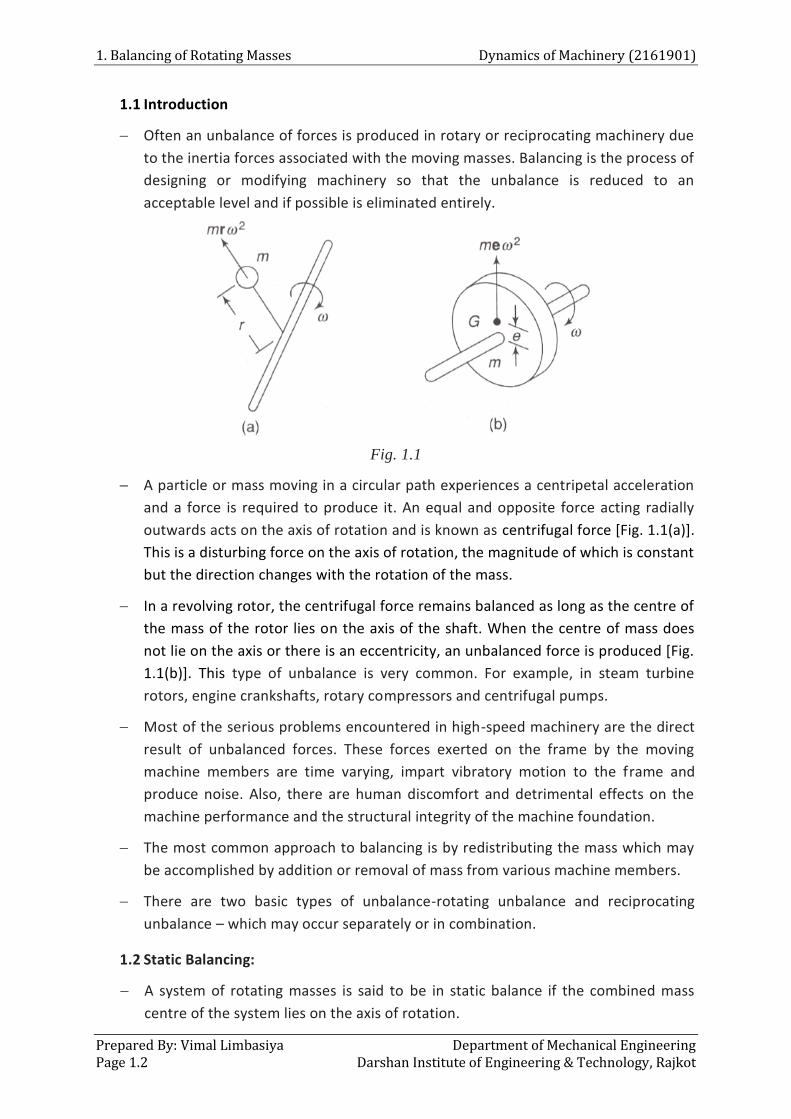
A particle or mass moving in a circular path experiences a centripetal acceleration
and a force is required to produce it. An equal and opposite force acting radially
outwards acts on the axis of rotation and is known as centrifugal force [Fig. 1.1(a)].
This is a disturbing force on the axis of rotation, the magnitude of which is constant
but the direction changes with the rotation of the mass.
In a revolving rotor, the centrifugal force remains balanced as long as the centre of
the mass of the rotor lies on the axis of the shaft. When the centre of mass does
not lie on the axis or there is an eccentricity, an unbalanced force is produced [Fig.
1.1(b)]. This type of unbalance is very common. For example, in steam turbine
rotors, engine crankshafts, rotary compressors and centrifugal pumps.
Most of the serious problems encountered in high-speed machinery are the direct
result of unbalanced forces. These forces exerted on the frame by the moving
machine members are time varying, impart vibratory motion to the frame and
produce noise. Also, there are human discomfort and detrimental effects on the
machine performance and the structural integrity of the machine foundation.
The most common approach to balancing is by redistributing the mass which may
be accomplished by addition or removal of mass from various machine members.
There are two basic types of unbalance-rotating unbalance and reciprocating
unbalance – which may occur separately or in combination.
1.2 Static Balancing:
A system of rotating masses is said to be in static balance if the combined mass
centre of the system lies on the axis of rotation.
Dynamics of Machinery (2161901) 1. Balancing of Rotating Masses
Department of Mechanical Engineering Prepared By: Vimal Limbasiya Darshan Institute of Engineering & Technology, Rajkot Page 1.3
1.3 Types of Balancing:
There are main two types of balancing conditions
(i) Balancing of rotating masses
(ii) Balancing of reciprocating masses
(i) Balancing of Rotating Masses
Whenever a certain mass is attached to a rotating shaft, it exerts some centrifugal
force, whose effect is to bend the shaft and to producevibrations in it. In order to prevent
the effect of centrifugal force, another mass is attached to the opposite side of theshaft,
at such a position so as to balance the effect of the centrifugal force of the first mass.
This is done in such away that the centrifugal forces of both the masses are made to be
equal and opposite. The process of providing the second mass in order to counteract the
effect of the centrifugal force of the first mass is called balancing of rotating masses.
The following cases are important from the subject point of view:
1. Balancing of a single rotating mass by a single mass rotating in the same plane.
2. Balancing of different masses rotating in the same plane.
3. Balancing of different masses rotating in different planes.
1.4 Balancing of Several Masses Rotating in the Same Plane
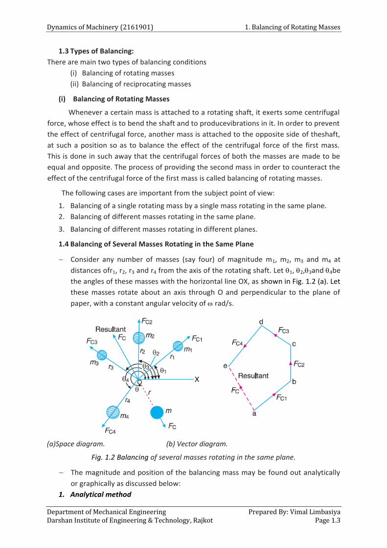
Consider any number of masses (say four) of magnitude m1, m2, m3 and m4 at
distances ofr1, r2, r3 and r4 from the axis of the rotating shaft. Let 1, 2,3and 4be
the angles of these masses with the horizontal line OX, as shown in Fig. 1.2 (a). Let
these masses rotate about an axis through O and perpendicular to the plane of
paper, with a constant angular velocity of rad/s.
(a)Space diagram. (b) Vector diagram.
Fig. 1.2 Balancing of several masses rotating in the same plane.
The magnitude and position of the balancing mass may be found out analytically
or graphically as discussed below:
1. Analytical method
1. Balancing of Rotating Masses Dynamics of Machinery (2161901)
Prepared By: Vimal Limbasiya Department of Mechanical Engineering Page 1.4 Darshan Institute of Engineering & Technology, Rajkot
Each mass produces a centrifugal force acting radially outwards from the axis of
rotation. Let F be the vector sum of these forces.
F = m1r12+ m2r2
2 +m3r32+ m4r4
2
The rotor is said to be statically balanced if the vector sum F is zero.
If F is not zero, i.e., the rotor is unbalanced, then produce a counterweight
(balance weight) of mass mc, at radius rc to balance the rotor so that
m1r12+ m2r2
2 +m3r32+ m4r4
2 + mcrc2 = 0
m1r1+ m2r2 +m3r3+ m4r4 + mcrc = 0
The magnitude of either mc or rc may be selected and of other can be calculated.
In general, if mr is the vector sum of m1.r1, m2.r2, m3.r3, m4.r4, etc., then
mr +mcrc = 0
To solve these equation by mathematically, divide each force into its x and z
components, mrcos + mcrccosc = 0
and mrsin +mcrcsinc= 0
mcrccosc= −mrcos…………………………(i)
and mcrcsinc= −mrsin............................(ii)
Squaring and adding (i) and (ii),
mcrc = 𝑚𝑟𝑐𝑜𝑠 ² + 𝑚𝑟𝑠𝑖𝑛 ²
Dividing (ii) by (i),
𝑡𝑎𝑛𝑐 =−𝑚𝑟𝑠𝑖𝑛
−𝑚𝑟𝑐𝑜𝑠
The signs of the numerator and denominator of this function identify the quadrant
of the angle.
2. Graphical method
First of all, draw the space diagram with the positions of the several masses, as
shown in Fig. 1.2 (a).
Find out the centrifugal force (or product of the mass and radius of rotation)
exerted byeach mass on the rotating shaft.
Now draw the vector diagram with the obtained centrifugal forces (or the product
of themasses and their radii of rotation), such that ab represents the centrifugal
force exerted by the mass m1 (or m1.r1) in magnitude and direction to some
suitable scale. Similarly, draw bc, cd and de to represent centrifugal forces of
other masses m2, m3 and m4 (or m2.r2,m3.r3 and m4.r4).
Now, as per polygon law of forces, the closing side ae represents the resultant
force inmagnitude and direction, as shown in Fig. 1.2 (b).
The balancing force is, then, equal to resultant force, but in opposite direction.
Dynamics of Machinery (2161901) 1. Balancing of Rotating Masses
Department of Mechanical Engineering Prepared By: Vimal Limbasiya Darshan Institute of Engineering & Technology, Rajkot Page 1.5
Now find out the magnitude of the balancing mass (m) at a given radius of
rotation (r), such that
m.r.2= Resultant centrifugal force
or m.r = Resultant of m1.r1, m2.r2, m3.r3 and m4.r4
(In general for graphical solution, vectors m1.r1, m2.r2, m3.r3, m4.r4, etc., are added. If
they close in a loop, the system is balanced. Otherwise, the closing vector will be
giving mc.rc. Its direction identifies the angular position of the countermass relative
to the other mass.)
Example 1.1 :A circular disc mounted on a shaft carries three attached masses of 4 kg, 3 kg
and 2.5 kg at radial distances of 75 mm, 85 mm and 50 mm and at the angular positions of
45°, 135° and 240° respectively. The angular positions are measured counterclockwise from
the reference line along the x-axis. Determine the amount of the countermass at a radial
distance of 75 mm required for the static balance.
m1 = 4 kg r1 = 75 mm 1 = 45°
m2 = 3 kg r2= 85 mm 2 = 135°
m3 = 2.5 kg r3 = 50 mm 3 = 240°
m1r1 = 4 x 75 = 300 kg.mm
m2r2 = 3 x 85 = 255 kg.mm
m3r3 = 2.5 x 50 = 125 kg.mm
Analytical Method:
mr +mcrc = 0
300 cos45°+ 255 cos135° + 125 cos240° + mcrccosc= 0 and
300 sin 45°+ 255 sin 135° + 125 sin 240° + mcrcsinc= 0
Squaring, adding and then solving,
2
2
(300 cos 45 255 cos 135 125 cos240 )
(300 sin45 255 sin 135 125 sin240 )C Cm r
2 275 ( 30.68) (284.2)Cm
= 285.8 kg.mm
mc = 3.81 kg
sin 284.2tan 9.26
cos ( 30.68)C
mr
mr
c = 83°50’
clies in the fourth quadrant (numerator is negative and denominator is positive).
c = 360 83°50’
c = 276°9’
Graphical Method:
1. Balancing of Rotating Masses Dynamics of Machinery (2161901)
Prepared By: Vimal Limbasiya Department of Mechanical Engineering Page 1.6 Darshan Institute of Engineering & Technology, Rajkot
The magnitude and the position of the balancing mass may also be found
graphically as discussed below :
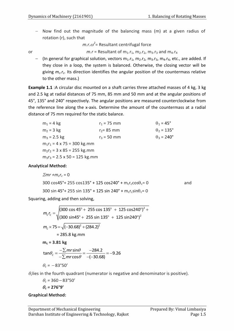
Now draw the vector diagram with the above values, to some suitable scale, as
shown in Fig. 1.3. The closing side of the polygon co represents the resultant force.
By measurement, we find that co = 285.84 kg-mm.
Fig. 1.3 Vector Diagram
The balancing force is equal to the resultant force. Since the balancing force is
proportional to m.r, therefore
mC× 75 = vector co = 285.84 kg-mm or mC = 285.84/75
mC = 3.81 kg.
By measurement we also find that the angle of inclination of the balancing mass (m)
from the horizontal or positive X-axis,
θC = 276°.
Example 1.2 :Four masses m1, m2, m3 and m4 are 200 kg, 300 kg, 240 kg and 260 kg
respectively. The corresponding radii of rotation are 0.2 m, 0.15 m, 0.25 m and 0.3 m
respectively and the angles between successive masses are 45°, 75° and 135°. Find the
position and magnitude of the balance mass required, if its radius of rotation is 0.2 m.
m1 = 200 kg r1 = 0.2 m 1 = 0°
m2 = 300 kg r2= 0.15 m 2 = 45°
m3 = 240 kg r3 = 0.25 m 3 = 45° +75° = 120°
m4 = 260 kg r4 = 0.3 m 4 = 120° + 135° = 255°
m1r1 = 200 x 0.2 = 40 rC = 0.2 m
m2r2 = 300 x 0.15 = 45
m3r3 = 240 x 0.25 = 60
m4r4 = 260 x 0.3 = 78
mr +mcrc = 0
40 cos0° + 45cos45°+ 60cos120° + 78cos255° + mcrccosc= 0 and
40 sin 0° + 45 sin 45°+ 60 sin 120° + 78 sin 255°+ mcrcsinc= 0
Squaring, adding and then solving,
Dynamics of Machinery (2161901) 1. Balancing of Rotating Masses
Department of Mechanical Engineering Prepared By: Vimal Limbasiya Darshan Institute of Engineering & Technology, Rajkot Page 1.7
2
2
(40cos0 45 cos45 60 cos 120 78 cos255 )
(40sin0 45 sin45 60 sin 120 78 sin255 )C Cm r
2 20.2 (21.6) (8.5)Cm
= 23.2 kg.mm
mc = 116 kg
sin 8.5tan 0.3935
cos 21.6C
mr
mr
c = 21°28’
clies in the third quadrant (numerator is negative and denominator is negative).
c = 180 +21°28’
c = 201°28’
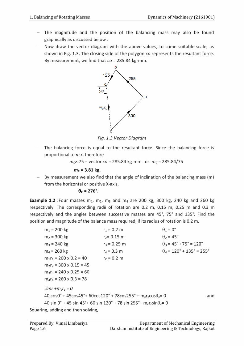
Graphical Method:
For graphical method draw the vector diagram with the above values, to some
suitable scale, as shown in Fig. 1.4. The closing side of the polygon ae represents
the resultant force. By measurement, we find that ae = 23 kg-m.
Fig. 1.4 Vector Diagram
The balancing force is equal to the resultant force.Since the balancing force is
proportional to m.r, therefore
m× 0.2 = vector ea= 23 kg-m or mC = 23/0.2
mC = 115 kg.
By measurement we also find that the angle of inclination of the balancing mass (m)
from the horizontal or positive X-axis,
θC = 201°.
1.5 Dynamic Balancing
1. Balancing of Rotating Masses Dynamics of Machinery (2161901)
Prepared By: Vimal Limbasiya Department of Mechanical Engineering Page 1.8 Darshan Institute of Engineering & Technology, Rajkot
When several masses rotate in different planes, the centrifugal forces,in addition
to being out ofbalance, also form couples. A system of rotating masses is in
dynamic balance when there does not exist anyresultant centrifugal force as well
as resultant couple.
In the work that follows, the products of mr and mrl (instead ofmr2 and mrl2),
usually, have been referred as force and couplerespectively as it is more
convenient to draw force and couplepolygons with these quantities.
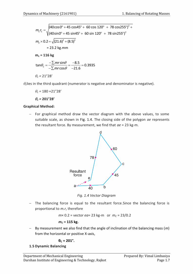
Fig. 1.5
If m1, and m2 are two masses (Fig. 1.5) revolving diametrically opposite to each
other in different planes such that m1r1= m2r2,the centrifugal forces are balanced,
but an unbalanced couple of magnitude m1r1l (= m2r2l) is introduced. The couple
acts in a plane that contains the axis of rotation and the two masses. Thus,
thecouple is of constant magnitude but variable direction.
1.6 Balancing of Several Masses Rotating in the different Planes
Let there be a rotor revolving with a uniform angular velocity . m1, m2and m3 are
the masses attached to the rotor at radii r1, r2 and r3respectively.The masses m1,
m2and m3rotate in planes1, 2 and 3 respectively. Choose a reference plane at O so
that the distances of the planes 1, 2 and 3 from O are l1, l2 and l3 respectively.
Transference of each unbalanced force to the reference plane introduces the like
number of forces and couples.
The unbalanced forces in the reference plane are m1r12, m2r2
2and m3r32 acting
radially outwards.
The unbalanced couples in the reference plane are m1r12l1, m2r2
2l2 andm3r32l3
which may be represented by vectors parallel to the respective force vectors, i.e.,
parallel to the respective radii of m1, m2and m3.
For complete balancing of the rotor, the resultant force and resultant couple both
should be zero, i.e., m1r12 + m2r2
2 + m3r32 = 0 …………………(a)
and m1r12l1 + m2r2
2l2+ m3r32l3 = 0 ...………………(b)
If the Eqs (a) and (b) are not satisfied, then there are unbalanced forces and
couples. A mass placed in the reference plane may satisfy the force equation but
the couple equation is satisfied only by two equal forces in different transverse
Dynamics of Machinery (2161901) 1. Balancing of Rotating Masses
Department of Mechanical Engineering Prepared By: Vimal Limbasiya Darshan Institute of Engineering & Technology, Rajkot Page 1.9
planes.
Thus in general, two planes are needed to balance a system of rotating masses.
Therefore, in order to satisfy Eqs (a) and (b), introduce two counter-masses mC1
and mC2 at radii rC1 and rC2 respectively. Then Eq. (a) may be written as
m1r12 + m2r2
2 + m3r32+mC1rC1
2 + mC2rC22 = 0
m1r1 + m2r2 + m3r3+mC1rC1 + mC2rC2 = 0
mr +mC1rC1 + mC2rC2 = 0 ………………….(c)
Let the two countermasses be placed in transverse planes at axial locations O and
Q, i.e., the countermassmC1 be placed in the reference plane and the distance of
the plane of mC2 be lC2 from the reference plane. Equation (b) modifies to (taking
moments about O)
m1r12l1 + m2r2
2l2+ m3r32l3+ mC2rC2
2lC2= 0
m1r1l1 + m2r2l2+ m3r3l3 + mC2rC2lC2= 0
mrl+ mC2rC2lC2= 0 …………………(d)
Thus, Eqs (c) and (d) are the necessary conditions for dynamic balancing of rotor.
Again the equations can be solved mathematically or graphically.
Dividing Eq. (d) into component form
mrlcos+ mC2rC2lC2 cosC2 = 0
mrl sin+ mC2rC2lC2 sinC2 = 0
mC2rC2lC2cosC2 = −mrlcos ……………………(i)
mC2rC2lC2sinC2= −mrl sin …………………..(ii)
Squaring and adding (i) and (ii)
mC2rC2lC2 = 𝑚𝑟𝑙𝑐𝑜𝑠 ² + 𝑚𝑟𝑙𝑠𝑖𝑛 ²
Dividing (ii) by (i),
𝑡𝑎𝑛𝐶2 =−𝑚𝑟𝑙𝑠𝑖𝑛
−𝑚𝑟𝑙𝑐𝑜𝑠
After obtaining the values of mC2 andC2 from the above equations, solve Eq. (c) by
taking its components,
mrcos +mC1rC1cosC1+ mC2rC2cosC2= 0
mrsin +mC1rC1 sinC1+ mC2rC2 sinC2= 0
mC1rC1cosC1= −( mrcos+ mC2rC2cosC2)
mC1rC1 sinC1 =−( mrsin+ mC2rC2 sinC2)
mC1rC1= 𝑚𝑟𝑐𝑜𝑠 + 𝑚𝐶2𝑟𝐶2𝑐𝑜𝑠𝐶2 ² + 𝑚𝑟𝑠𝑖𝑛 + 𝑚𝐶2𝑟𝐶2𝑠𝑖𝑛𝐶2 ²
𝑡𝑎𝑛𝐶1 =− 𝑚𝑟𝑠𝑖𝑛 + 𝑚𝐶2𝑟𝐶2𝑠𝑖𝑛𝐶2
− 𝑚𝑟𝑐𝑜𝑠 + 𝑚𝐶2𝑟𝐶2𝑐𝑜𝑠𝐶2
1. Balancing of Rotating Masses Dynamics of Machinery (2161901)
Prepared By: Vimal Limbasiya Department of Mechanical Engineering Page 1.10 Darshan Institute of Engineering & Technology, Rajkot
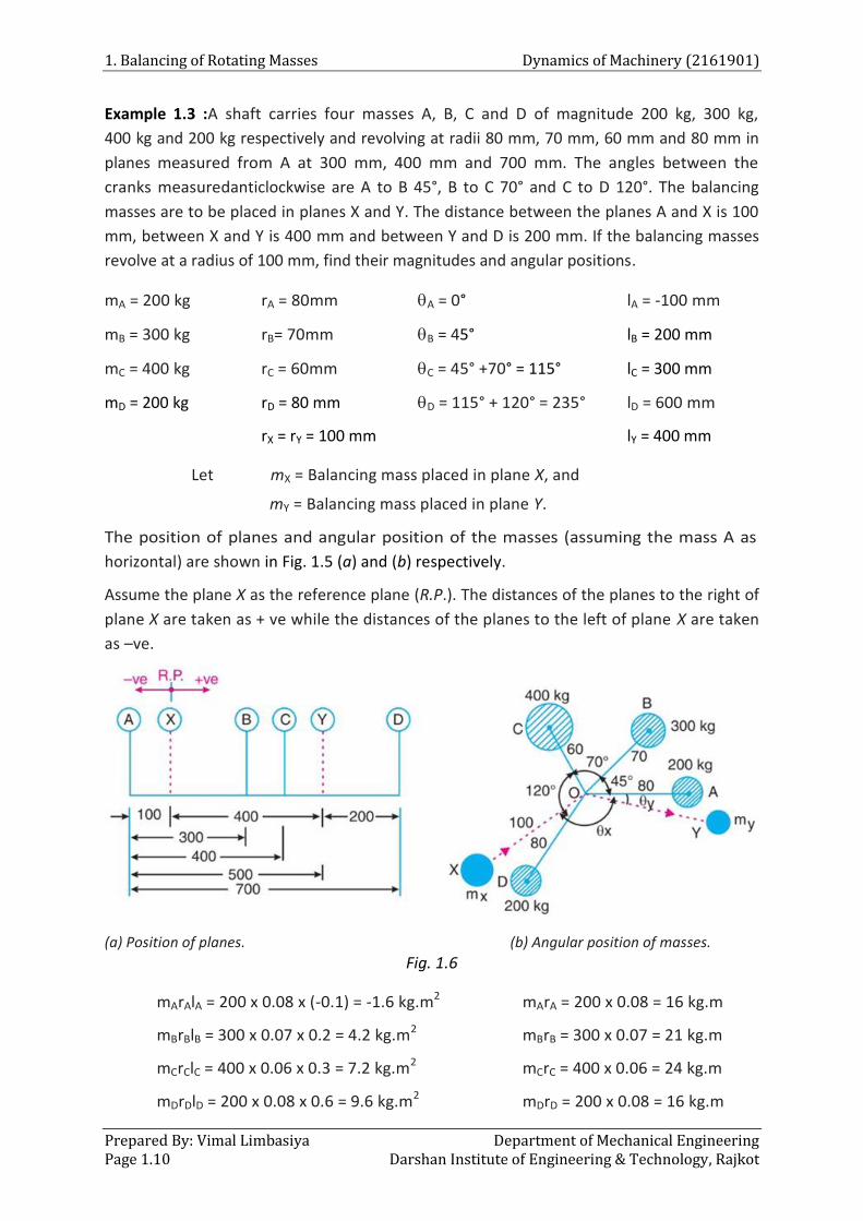
Example 1.3 :A shaft carries four masses A, B, C and D of magnitude 200 kg, 300 kg,
400 kg and 200 kg respectively and revolving at radii 80 mm, 70 mm, 60 mm and 80 mm in
planes measured from A at 300 mm, 400 mm and 700 mm. The angles between the
cranks measuredanticlockwise are A to B 45°, B to C 70° and C to D 120°. The balancing
masses are to be placed in planes X and Y. The distance between the planes A and X is 100
mm, between X and Y is 400 mm and between Y and D is 200 mm. If the balancing masses
revolve at a radius of 100 mm, find their magnitudes and angular positions.
mA = 200 kg rA = 80mm A = 0° lA = -100 mm
mB = 300 kg rB= 70mm B = 45° lB = 200 mm
mC = 400 kg rC = 60mm C = 45° +70° = 115° lC = 300 mm
mD = 200 kg rD = 80 mm D = 115° + 120° = 235° lD = 600 mm
rX = rY = 100 mm lY = 400 mm
Let mX = Balancing mass placed in plane X, and
mY = Balancing mass placed in plane Y.
The position of planes and angular position of the masses (assuming the mass A as
horizontal) are shown in Fig. 1.5 (a) and (b) respectively.
Assume the plane X as the reference plane (R.P.). The distances of the planes to the right of
plane X are taken as + ve while the distances of the planes to the left of plane X are taken
as –ve.
(a) Position of planes. (b) Angular position of masses.
Fig. 1.6
mArAlA = 200 x 0.08 x (-0.1) = -1.6 kg.m2 mArA = 200 x 0.08 = 16 kg.m
mBrBlB = 300 x 0.07 x 0.2 = 4.2 kg.m2 mBrB = 300 x 0.07 = 21 kg.m
mCrClC = 400 x 0.06 x 0.3 = 7.2 kg.m2 mCrC = 400 x 0.06 = 24 kg.m
mDrDlD = 200 x 0.08 x 0.6 = 9.6 kg.m2 mDrD = 200 x 0.08 = 16 kg.m
Dynamics of Machinery (2161901) 1. Balancing of Rotating Masses
Department of Mechanical Engineering Prepared By: Vimal Limbasiya Darshan Institute of Engineering & Technology, Rajkot Page 1.11
Analytical Method:
For unbalanced couple
mrl +mYrYlY = 0
2 2( cos ) ( sin )Y Y Ym r l mrl mrl
2
2
( 1.6cos0 4.2cos45 7.2cos115 9.6cos235 )
( 1.6sin0 4.2sin45 7.2sin115 9.6sin235 )Y Y Ym r l
2 2( 7.179) (1.63)Y Y Ym r l
0.1 0.4 7.36Ym
mY = 184 kg.
sin 1.63tan 0.227
cos ( 7.179)Y
mrl
mrl
Y = 12°47’
Y lies in the fourth quadrant (numerator is negative and denominator is positive).
Y = 360 12°47’
Y = 347°12’
For unbalanced centrifugal force
mr +mXrX+ mYrY = 0
2 2( cos cos ) ( sin sin )X X Y Y Y Y Y Ym r mr m r mr m r
2
2
(16cos0 21cos45 24cos115 16cos235 18.4cos347 12')
(16sin0 21sin45 24sin115 16sin235 18.4sin347 12')X Xm r
2 2(29.47) (19.42)X Xm r
0.1 35.29Xm
Xm = 353 kg.
sin 19.42tan 0.6589
cos 29.47X
mr
mr
X = 33°22’
Xlies in the third quadrant (numerator is negative and denominator is negative).
X = 180 +33°22’
X = 213°22’
Graphical Method:
The balancing masses and their angular positions may be determined graphically as
discussed below :
1. Balancing of Rotating Masses Dynamics of Machinery (2161901)
Prepared By: Vimal Limbasiya Department of Mechanical Engineering Page 1.12 Darshan Institute of Engineering & Technology, Rajkot
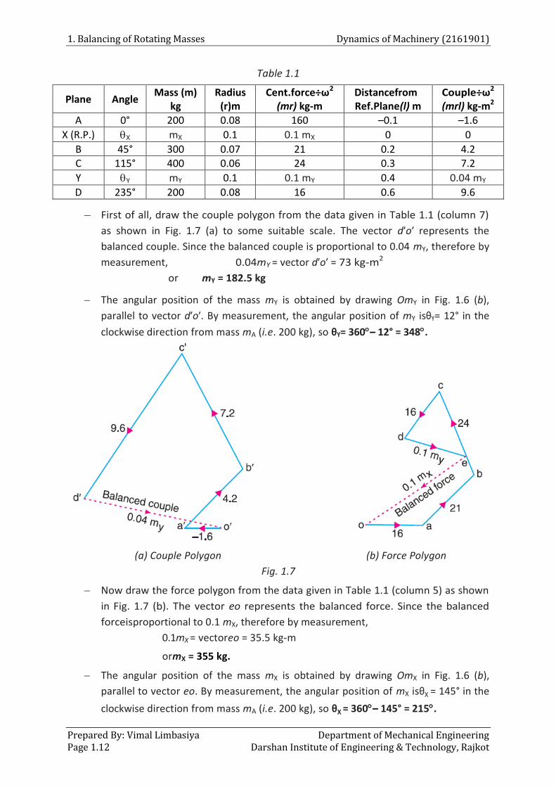
Table 1.1
Plane Angle Mass (m)
kg Radius
(r)m Cent.force÷ω2
(mr) kg-m Distancefrom Ref.Plane(l) m
Couple÷ω2
(mrl) kg-m2
A 0° 200 0.08 160 –0.1 –1.6
X (R.P.) X mX 0.1 0.1 mX 0 0
B 45° 300 0.07 21 0.2 4.2
C 115° 400 0.06 24 0.3 7.2
Y Y mY 0.1 0.1 mY 0.4 0.04 mY
D 235° 200 0.08 16 0.6 9.6
First of all, draw the couple polygon from the data given in Table 1.1 (column 7)
as shown in Fig. 1.7 (a) to some suitable scale. The vector d′o′ represents the
balanced couple. Since the balanced couple is proportional to 0.04 mY, therefore by
measurement, 0.04mY = vector d′o′ = 73 kg-m2
or mY = 182.5 kg
The angular position of the mass mY is obtained by drawing OmY in Fig. 1.6 (b),
parallel to vector d′o′. By measurement, the angular position of mY isθY= 12° in the
clockwise direction from mass mA (i.e. 200 kg), so θY= 360– 12° = 348.
(a) Couple Polygon (b) Force Polygon
Fig. 1.7
Now draw the force polygon from the data given in Table 1.1 (column 5) as shown
in Fig. 1.7 (b). The vector eo represents the balanced force. Since the balanced
forceisproportional to 0.1 mX, therefore by measurement,
0.1mX = vectoreo = 35.5 kg-m
ormX = 355 kg.
The angular position of the mass mX is obtained by drawing OmX in Fig. 1.6 (b),
parallel to vector eo. By measurement, the angular position of mX isθX = 145° in the
clockwise direction from mass mA (i.e. 200 kg), so θX = 360– 145° = 215.
Dynamics of Machinery (2161901) 1. Balancing of Rotating Masses
Department of Mechanical Engineering Prepared By: Vimal Limbasiya Darshan Institute of Engineering & Technology, Rajkot Page 1.13
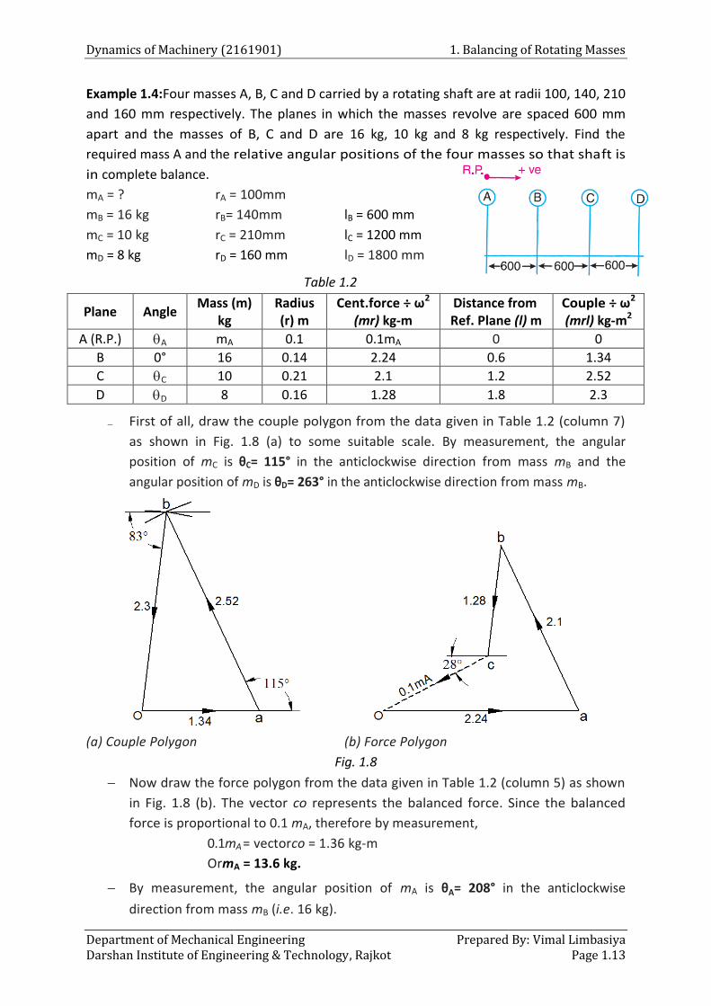
Example 1.4:Four masses A, B, C and D carried by a rotating shaft are at radii 100, 140, 210
and 160 mm respectively. The planes in which the masses revolve are spaced 600 mm
apart and the masses of B, C and D are 16 kg, 10 kg and 8 kg respectively. Find the
required mass A and the relative angular positions of the four masses so that shaft is
in complete balance.
mA = ? rA = 100mm
mB = 16 kg rB= 140mm lB = 600 mm
mC = 10 kg rC = 210mm lC = 1200 mm
mD = 8 kg rD = 160 mm lD = 1800 mm
Table 1.2
Plane Angle Mass (m)
kg Radius (r) m
Cent.force ÷ ω2
(mr) kg-m Distance from Ref. Plane (l) m
Couple ÷ ω2
(mrl) kg-m2
A (R.P.) A mA 0.1 0.1mA 0 0
B 0° 16 0.14 2.24 0.6 1.34
C C 10 0.21 2.1 1.2 2.52
D D 8 0.16 1.28 1.8 2.3
First of all, draw the couple polygon from the data given in Table 1.2 (column 7)
as shown in Fig. 1.8 (a) to some suitable scale. By measurement, the angular
position of mC is θC= 115° in the anticlockwise direction from mass mB and the
angular position of mD is θD= 263° in the anticlockwise direction from mass mB.
(a) Couple Polygon (b) Force Polygon
Fig. 1.8
Now draw the force polygon from the data given in Table 1.2 (column 5) as shown
in Fig. 1.8 (b). The vector co represents the balanced force. Since the balanced
force is proportional to 0.1 mA, therefore by measurement,
0.1mA = vectorco = 1.36 kg-m
OrmA = 13.6 kg.
By measurement, the angular position of mA is θA= 208° in the anticlockwise
direction from mass mB (i.e. 16 kg).
1. Balancing of Rotating Masses Dynamics of Machinery (2161901)
Prepared By: Vimal Limbasiya Department of Mechanical Engineering Page 1.14 Darshan Institute of Engineering & Technology, Rajkot
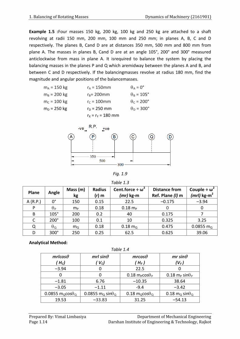
Example 1.5 :Four masses 150 kg, 200 kg, 100 kg and 250 kg are attached to a shaft
revolving at radii 150 mm, 200 mm, 100 mm and 250 mm; in planes A, B, C and D
respectively. The planes B, Cand D are at distances 350 mm, 500 mm and 800 mm from
plane A. The masses in planes B, Cand D are at an angle 105°, 200° and 300° measured
anticlockwise from mass in plane A. It isrequired to balance the system by placing the
balancing masses in the planes P and Q which aremidway between the planes A and B, and
between C and D respectively. If the balancingmasses revolve at radius 180 mm, find the
magnitude and angular positions of the balancemasses.
mA = 150 kg rA = 150mm A = 0°
mB = 200 kg rB= 200mm B = 105°
mC = 100 kg rC = 100mm C = 200°
mD = 250 kg rD = 250 mm D = 300°
rX = rY = 180 mm
Fig. 1.9
Table 1.3
Plane Angle Mass (m)
kg Radius (r) m
Cent.force ÷ ω2
(mr) kg-m Distance from Ref. Plane (l) m
Couple ÷ ω2
(mrl) kg-m2
A (R.P.) 0° 150 0.15 22.5 –0.175 –3.94
P P mP 0.18 0.18 mP 0 0
B 105° 200 0.2 40 0.175 7
C 200° 100 0.1 10 0.325 3.25
Q Q mQ 0.18 0.18 mQ 0.475 0.0855 mQ
D 300° 250 0.25 62.5 0.625 39.06
Analytical Method:
Table 1.4
mrlcos ( HC)
mrl sin ( VC)
mrcos ( HF )
mr sin (VF )
–3.94 0 22.5 0
0 0 0.18 mPcosP 0.18 mP sinP
–1.81 6.76 –10.35 38.64
–3.05 –1.11 -9.4 –3.42
0.0855 mQcosQ 0.0855 mQ sinQ 0.18 mQcosQ 0.18 mQ sinQ
19.53 –33.83 31.25 –54.13
Dynamics of Machinery (2161901) 1. Balancing of Rotating Masses
Department of Mechanical Engineering Prepared By: Vimal Limbasiya Darshan Institute of Engineering & Technology, Rajkot Page 1.15
HC = 0
–3.94 + 0 – 1.81 – 3.05 + 0.0855 mQcosQ + 19.53 = 0
0.0855 mQcosQ = – 10.73
mQcosQ = – 125.497 …………………..(i)
VC = 0
0 + 0 + 6.76 – 1.11 + 0.0855 mQ sinQ – 33.83 = 0
0.0855 mQ sinQ = 28.18
mQ sinQ = 329.59 ………………..(ii)
2 2( 125.497) (329.59)Qm
mQ = 352.67 kg.
sin 329.59
cos 125.497Q Q
Q Q
m
m
tanQ = – 2.626
Q = – 69.15
Q = 180 – 69.15
Q = 110.84°
HF = 0
22.5 + 0.18 mPcosP – 10.35 – 9.4 + 0.18 mQcosQ + 31.25 = 0
22.5 + 0.18 mPcosP – 10.35 – 9.4 + 0.18 (352.67) cos 110.84° + 31.25 = 0
0.18 mPcosP = – 11.416
mPcosP = – 63.42
VF = 0
0 + 0.18 mP sinP + 38.64 – 3.42 + 0.18 mQ sinQ – 54.13 = 0
0 + 0.18 mP sinP + 38.64 – 3.42 + 0.18 (352.67) sin 110.84° – 54.13 = 0
0.18 mP sinP = – 40.417
mP sinP = – 224.54
2 2( 63.42) ( 224.54)Pm
mP = 233.32 kg.
sin 224.54
cos 63.42P P
P P
m
m
tanP = 3.54
P = 74.23
P = 180 + 74.23
P = 254.23°
1. Balancing of Rotating Masses Dynamics of Machinery (2161901)
Prepared By: Vimal Limbasiya Department of Mechanical Engineering Page 1.16 Darshan Institute of Engineering & Technology, Rajkot
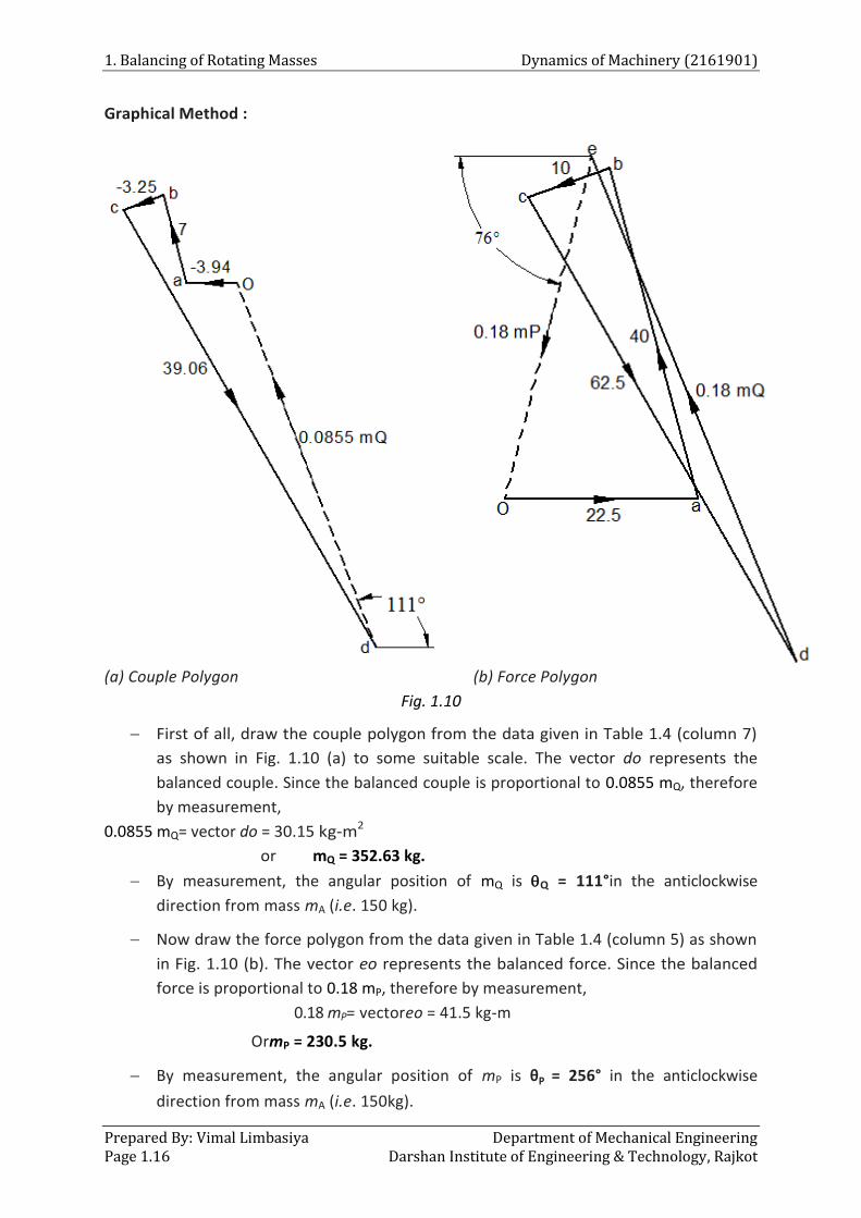
Graphical Method :
(a) Couple Polygon (b) Force Polygon
Fig. 1.10
First of all, draw the couple polygon from the data given in Table 1.4 (column 7)
as shown in Fig. 1.10 (a) to some suitable scale. The vector do represents the
balanced couple. Since the balanced couple is proportional to 0.0855 mQ, therefore
by measurement,
0.0855 mQ= vector do = 30.15 kg-m2
or mQ = 352.63 kg.
By measurement, the angular position of mQ is Q = 111°in the anticlockwise
direction from mass mA (i.e. 150 kg).
Now draw the force polygon from the data given in Table 1.4 (column 5) as shown
in Fig. 1.10 (b). The vector eo represents the balanced force. Since the balanced
force is proportional to 0.18 mP, therefore by measurement,
0.18 mP= vectoreo = 41.5 kg-m
OrmP = 230.5 kg.
By measurement, the angular position of mP is θP = 256° in the anticlockwise
direction from mass mA (i.e. 150kg).
Dynamics of Machinery (2161901) 1. Balancing of Rotating Masses
Department of Mechanical Engineering Prepared By: Vimal Limbasiya Darshan Institute of Engineering & Technology, Rajkot Page 1.17
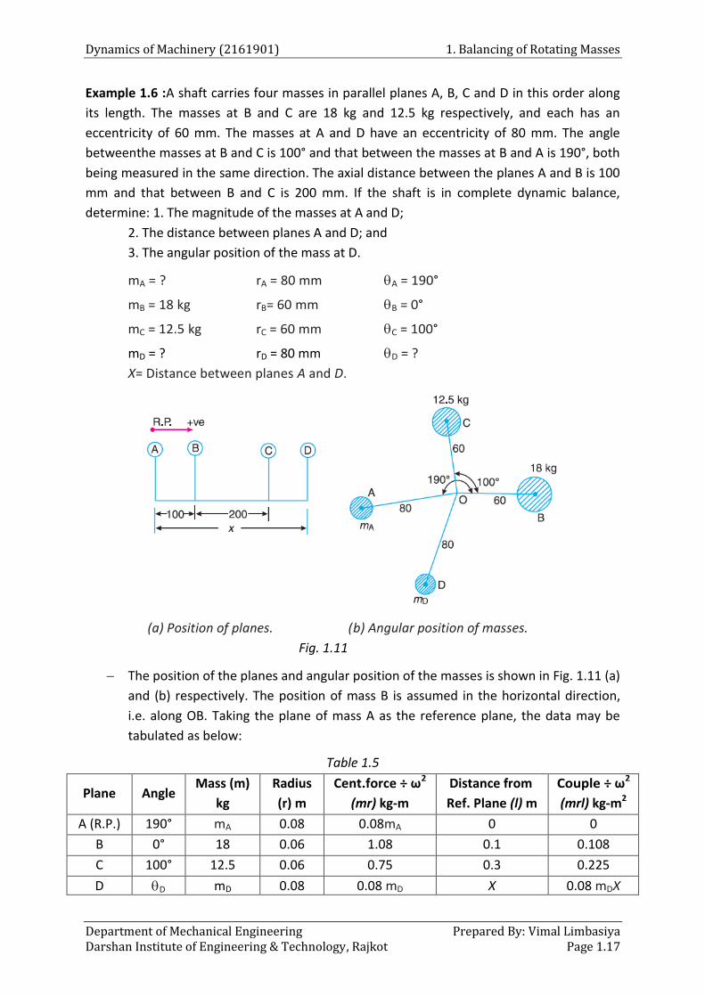
Example 1.6 :A shaft carries four masses in parallel planes A, B, C and D in this order along
its length. The masses at B and C are 18 kg and 12.5 kg respectively, and each has an
eccentricity of 60 mm. The masses at A and D have an eccentricity of 80 mm. The angle
betweenthe masses at B and C is 100° and that between the masses at B and A is 190°, both
being measured in the same direction. The axial distance between the planes A and B is 100
mm and that between B and C is 200 mm. If the shaft is in complete dynamic balance,
determine: 1. The magnitude of the masses at A and D;
2. The distance between planes A and D; and
3. The angular position of the mass at D.
mA = ? rA = 80 mm A = 190°
mB = 18 kg rB= 60 mm B = 0°
mC = 12.5 kg rC = 60 mm C = 100°
mD = ? rD = 80 mm D = ?
X= Distance between planes A and D.
(a) Position of planes. (b) Angular position of masses.
Fig. 1.11
The position of the planes and angular position of the masses is shown in Fig. 1.11 (a)
and (b) respectively. The position of mass B is assumed in the horizontal direction,
i.e. along OB. Taking the plane of mass A as the reference plane, the data may be
tabulated as below:
Table 1.5
Plane Angle Mass (m)
kg
Radius
(r) m
Cent.force ÷ ω2
(mr) kg-m
Distance from
Ref. Plane (l) m
Couple ÷ ω2
(mrl) kg-m2
A (R.P.) 190° mA 0.08 0.08mA 0 0
B 0° 18 0.06 1.08 0.1 0.108
C 100° 12.5 0.06 0.75 0.3 0.225
D D mD 0.08 0.08 mD X 0.08 mDX
1. Balancing of Rotating Masses Dynamics of Machinery (2161901)
Prepared By: Vimal Limbasiya Department of Mechanical Engineering Page 1.18 Darshan Institute of Engineering & Technology, Rajkot
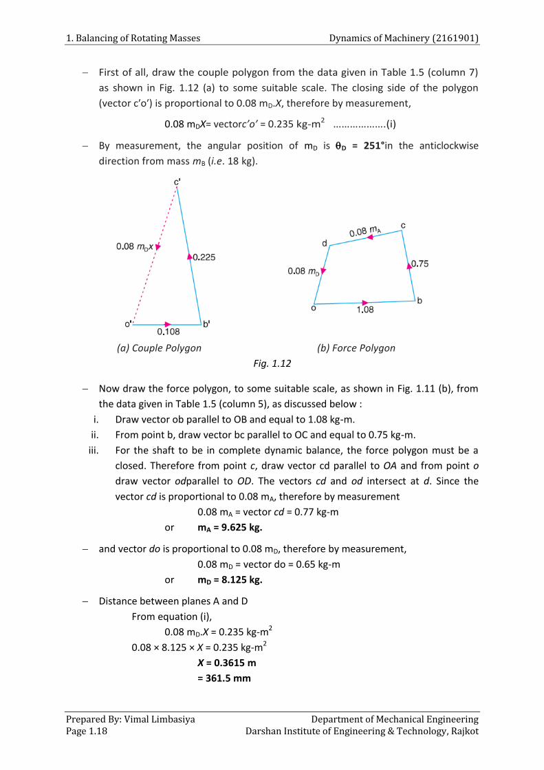
First of all, draw the couple polygon from the data given in Table 1.5 (column 7)
as shown in Fig. 1.12 (a) to some suitable scale. The closing side of the polygon
(vector c′o′) is proportional to 0.08 mD.X, therefore by measurement,
0.08 mDX= vectorc’o’ = 0.235 kg-m2 ……………….(i)
By measurement, the angular position of mD is D = 251°in the anticlockwise
direction from mass mB (i.e. 18 kg).
(a) Couple Polygon (b) Force Polygon
Fig. 1.12
Now draw the force polygon, to some suitable scale, as shown in Fig. 1.11 (b), from
the data given in Table 1.5 (column 5), as discussed below :
i. Draw vector ob parallel to OB and equal to 1.08 kg-m.
ii. From point b, draw vector bc parallel to OC and equal to 0.75 kg-m.
iii. For the shaft to be in complete dynamic balance, the force polygon must be a
closed. Therefore from point c, draw vector cd parallel to OA and from point o
draw vector odparallel to OD. The vectors cd and od intersect at d. Since the
vector cd is proportional to 0.08 mA, therefore by measurement
0.08 mA = vector cd = 0.77 kg-m
or mA = 9.625 kg.
and vector do is proportional to 0.08 mD, therefore by measurement,
0.08 mD = vector do = 0.65 kg-m
or mD = 8.125 kg.
Distance between planes A and D
From equation (i),
0.08 mD.X = 0.235 kg-m2
0.08 × 8.125 × X = 0.235 kg-m2
X = 0.3615 m
= 361.5 mm
Dynamics of Machinery (2161901) 1. Balancing of Rotating Masses
Department of Mechanical Engineering Prepared By: Vimal Limbasiya Darshan Institute of Engineering & Technology, Rajkot Page 1.19
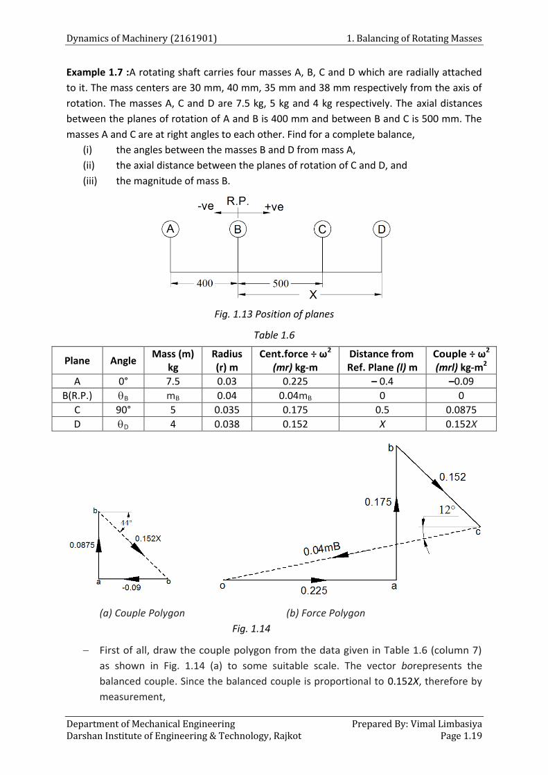
Example 1.7 :A rotating shaft carries four masses A, B, C and D which are radially attached
to it. The mass centers are 30 mm, 40 mm, 35 mm and 38 mm respectively from the axis of
rotation. The masses A, C and D are 7.5 kg, 5 kg and 4 kg respectively. The axial distances
between the planes of rotation of A and B is 400 mm and between B and C is 500 mm. The
masses A and C are at right angles to each other. Find for a complete balance,
(i) the angles between the masses B and D from mass A,
(ii) the axial distance between the planes of rotation of C and D, and
(iii) the magnitude of mass B.
Fig. 1.13 Position of planes
Table 1.6
Plane Angle Mass (m)
kg Radius (r) m
Cent.force ÷ ω2
(mr) kg-m Distance from Ref. Plane (l) m
Couple ÷ ω2
(mrl) kg-m2
A 0° 7.5 0.03 0.225 – 0.4 –0.09
B(R.P.) B mB 0.04 0.04mB 0 0
C 90° 5 0.035 0.175 0.5 0.0875
D D 4 0.038 0.152 X 0.152X
(a) Couple Polygon (b) Force Polygon
Fig. 1.14
First of all, draw the couple polygon from the data given in Table 1.6 (column 7)
as shown in Fig. 1.14 (a) to some suitable scale. The vector borepresents the
balanced couple. Since the balanced couple is proportional to 0.152X, therefore by
measurement,
1. Balancing of Rotating Masses Dynamics of Machinery (2161901)
Prepared By: Vimal Limbasiya Department of Mechanical Engineering Page 1.20 Darshan Institute of Engineering & Technology, Rajkot
0.152X = vectorbo
= 0.13 kg-m2
or X = 0.855 m.
The axial distance between the planes of rotation of C and D = 855 – 500 = 355 mm
By measurement, the angular position of mD is D = 360°– 44° = 316°in the
anticlockwise direction from mass mA (i.e. 7.5 kg).
Now draw the force polygon from the data given in Table 1.6 (column 5) as shown
in Fig. 1.14 (b). The vector co represents the balanced force. Since the balanced
force isproportional to 0.04 mB, therefore by measurement,
0.04 mB= vectorco
= 0.34 kg-m
or mB = 8.5 kg.
By measurement, the angular position of mB is θB = 180° + 12° = 192° in the
anticlockwise direction from mass mA (i.e. 7.5 kg).
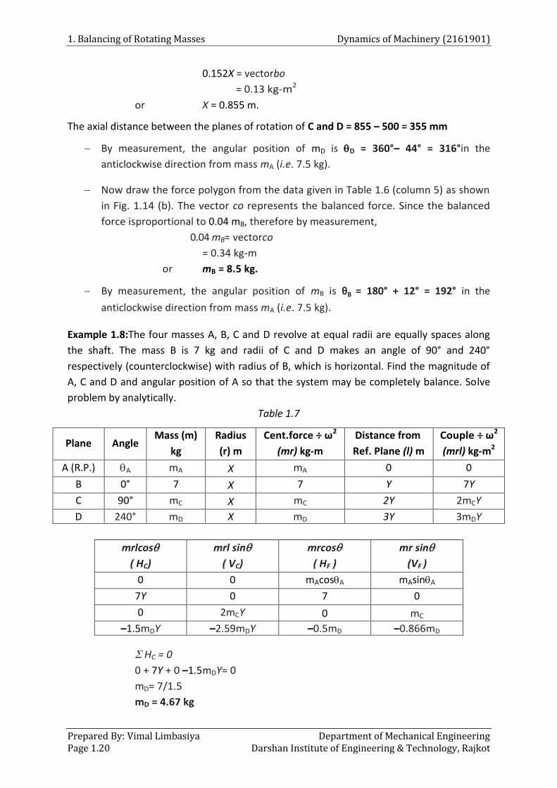
Example 1.8:The four masses A, B, C and D revolve at equal radii are equally spaces along
the shaft. The mass B is 7 kg and radii of C and D makes an angle of 90° and 240°
respectively (counterclockwise) with radius of B, which is horizontal. Find the magnitude of
A, C and D and angular position of A so that the system may be completely balance. Solve
problem by analytically.
Table 1.7
Plane Angle Mass (m)
kg
Radius
(r) m
Cent.force ÷ ω2
(mr) kg-m
Distance from
Ref. Plane (l) m
Couple ÷ ω2
(mrl) kg-m2
A (R.P.) A mA X mA 0 0
B 0° 7 X 7 Y 7Y
C 90° mC X mC 2Y 2mCY
D 240° mD X mD 3Y 3mDY
mrlcos
( HC)
mrl sin
( VC)
mrcos
( HF )
mr sin
(VF )
0 0 mAcosA mAsinA
7Y 0 7 0
0 2mCY 0 mC
–1.5mDY –2.59mDY –0.5mD –0.866mD
HC = 0
0 + 7Y + 0 –1.5mDY= 0
mD= 7/1.5
mD = 4.67 kg
Dynamics of Machinery (2161901) 1. Balancing of Rotating Masses
Department of Mechanical Engineering Prepared By: Vimal Limbasiya Darshan Institute of Engineering & Technology, Rajkot Page 1.21
VC = 0
0 + 0 + 2mCY–2.59mDY= 0
mC= 6.047 kg
HF = 0
mAcosA + 7 + 0 – 0.5mD = 0
mAcosA= – 4.665
VF = 0
mAsinA + 0 + mC– 0.866mD = 0
mAsinA = – 2.00278
2 2( 4.665) ( 2.00278)Am
mA = 5.076 kg
sin 2.00278tan 0.43
cos 4.665A A
A
A A
m
m
θA = 23.23°
θA = 180° + 23.23°
θA= 203.23°
1.7 Balancing Machines
A balancing machine is able to indicate whether a part is in balance or not and if it is
not, then it measures the unbalance by indicating its magnitude and location.
1.7.1. Static Balancing Machines
Static balancing machines are helpful for parts of small axial dimensions such as fans,
gears and impellers, etc., in which the mass lies practically in a single plane.
There are two machine which are used as static balancing machine: Pendulum type
balancing machine and Cradle type balancing machine.
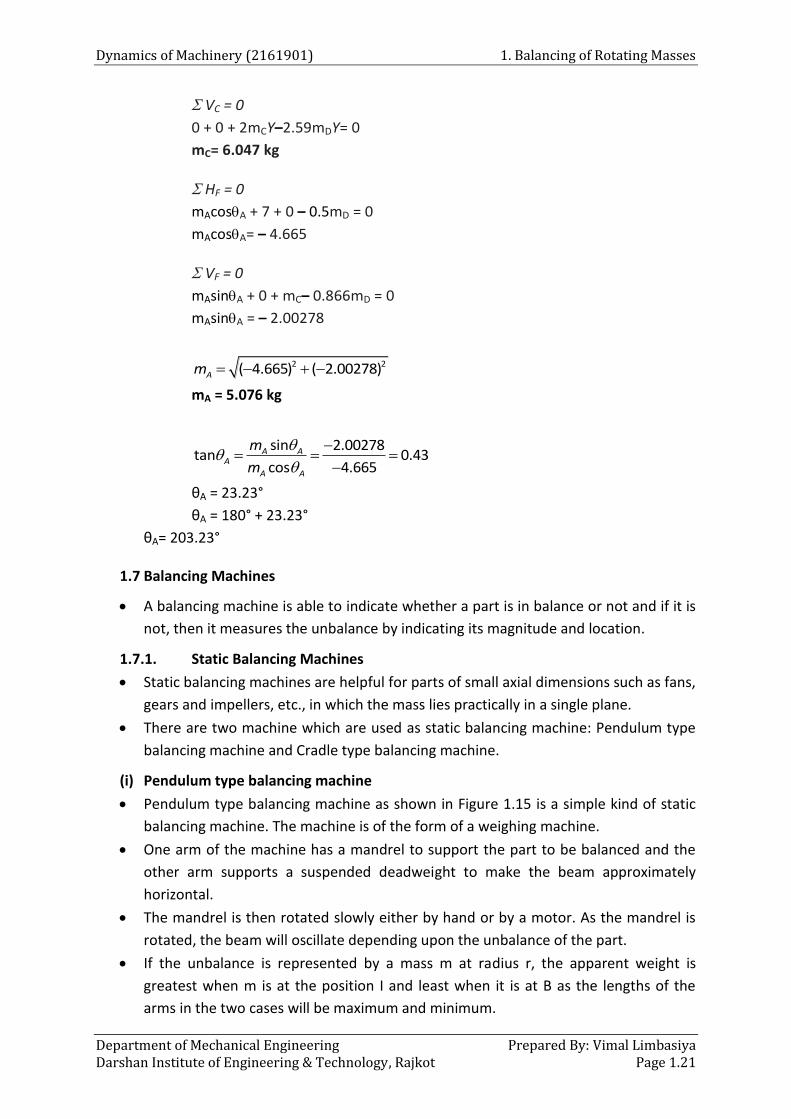
(i) Pendulum type balancing machine
Pendulum type balancing machine as shown in Figure 1.15 is a simple kind of static
balancing machine. The machine is of the form of a weighing machine.
One arm of the machine has a mandrel to support the part to be balanced and the
other arm supports a suspended deadweight to make the beam approximately
horizontal.
The mandrel is then rotated slowly either by hand or by a motor. As the mandrel is
rotated, the beam will oscillate depending upon the unbalance of the part.
If the unbalance is represented by a mass m at radius r, the apparent weight is
greatest when m is at the position I and least when it is at B as the lengths of the
arms in the two cases will be maximum and minimum.
1. Balancing of Rotating Masses Dynamics of Machinery (2161901)
Prepared By: Vimal Limbasiya Department of Mechanical Engineering Page 1.22 Darshan Institute of Engineering & Technology, Rajkot
A calibrated scale along with the pointer can also be used to measure the amount of
unbalance. Obviously, the pointer remains stationary in case the body is statically
balanced.
Fig. 1.15
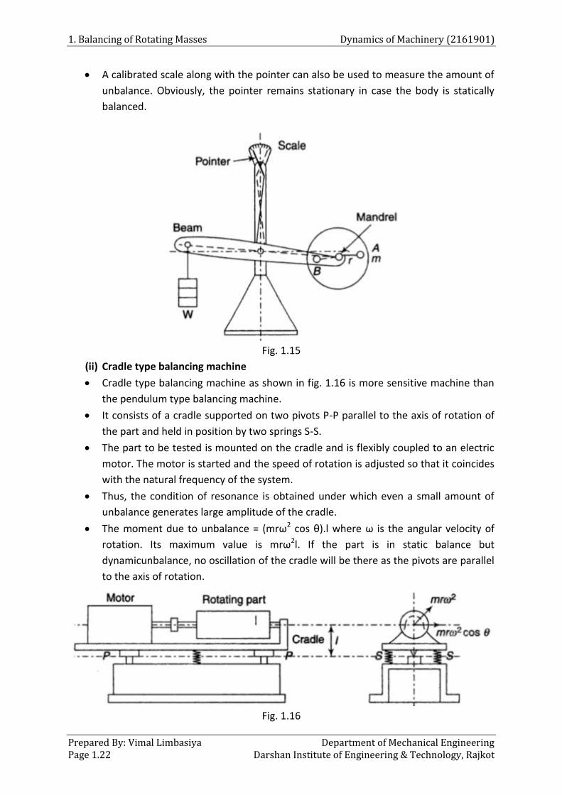
(ii) Cradle type balancing machine
Cradle type balancing machine as shown in fig. 1.16 is more sensitive machine than
the pendulum type balancing machine.
It consists of a cradle supported on two pivots P-P parallel to the axis of rotation of
the part and held in position by two springs S-S.
The part to be tested is mounted on the cradle and is flexibly coupled to an electric
motor. The motor is started and the speed of rotation is adjusted so that it coincides
with the natural frequency of the system.
Thus, the condition of resonance is obtained under which even a small amount of
unbalance generates large amplitude of the cradle.
The moment due to unbalance = (mrω2 cos θ).l where ω is the angular velocity of
rotation. Its maximum value is mrω2l. If the part is in static balance but
dynamicunbalance, no oscillation of the cradle will be there as the pivots are parallel
to the axis of rotation.
Fig. 1.16
Dynamics of Machinery (2161901) 1. Balancing of Rotating Masses
Department of Mechanical Engineering Prepared By: Vimal Limbasiya Darshan Institute of Engineering & Technology, Rajkot Page 1.23
1.7.2. Dynamic Balancing Machines
For dynamic balancing of a rotor, two balancing or countermasses are required to be
used in any two convenient planes. This implies that the complete unbalance of any
rotor system can be represented by two unbalances in those two planes.
Balancing is achieved by addition or removal of masses in these two planes,
whichever is convenient. The following is a common type of dynamic balancing
machine.
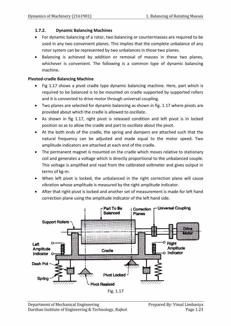
Pivoted-cradle Balancing Machine
Fig 1.17 shows a pivot cradle type dynamic balancing machine. Here, part which is
required to be balanced is to be mounted on cradle supported by supported rollers
and it is connected to drive motor through universal coupling.
Two planes are selected for dynamic balancing as shown in fig. 1.17 where pivots are
provided about which the cradle is allowed to oscillate.
As shown in fig 1.17, right pivot is released condition and left pivot is in locked
position so as to allow the cradle and part to oscillate about the pivot.
At the both ends of the cradle, the spring and dampers are attached such that the
natural frequency can be adjusted and made equal to the motor speed. Two
amplitude indicators are attached at each end of the cradle.
The permanent magnet is mounted on the cradle which moves relative to stationary
coil and generates a voltage which is directly proportional to the unbalanced couple.
This voltage is amplified and read from the calibrated voltmeter and gives output in
terms of kg-m.
When left pivot is locked, the unbalanced in the right correction plane will cause
vibration whose amplitude is measured by the right amplitude indicator.
After that right pivot is locked and another set of measurement is made for left hand
correction plane using the amplitude indicator of the left hand side.
Fig. 1.17
Department of Mechanical Engineering Prepared By: VimalLimbasiya Darshan Institute of Engineering & Technology, Rajkot Page 2.1
2 DYNANICS OF RECIPROCATING ENGINES
Course Contents
2.1 Slider Crank Kinematics
(Analytical)
2.2 Gas Force and Gas Torque
2.3 Inertia and Shaking Forces
2.4 Inertia and Shaking Torques
2.5 Dynamically Equivalent
Systems
2.6 Pin Forces in the Single
Cylinder Engine
2.7 Balancing of unbalanced
forces in reciprocating
masses
2.8 Balancing of Locomotives
2.9 Balancing of Multi Cylinder
Engine
2.10 Balancing of V – Engine
2.11 Balancing of Radial Engine
2. Dynamics of Reciprocating Engines Dynamics of Machinery (2161901)
Prepared By: Vimal Limbasiya Department of Mechanical Engineering Page 2.2 Darshan Institute of Engineering & Technology, Rajkot
2.1 Slider Crank Kinematics (Analytical)
There are many applications where moving parts are having reciprocating motion. For
example, IC engine, shaper machine, air compressors and many more where parts are in
reciprocating motion where they are subjected to continuous acceleration and
retardation.
Due to this motion, inertia force acts in the opposite direction of acceleration of the
moving parts. This opposite direction force which is termed as inertia force is the
unbalanced dynamic force which is acting on the reciprocating parts.
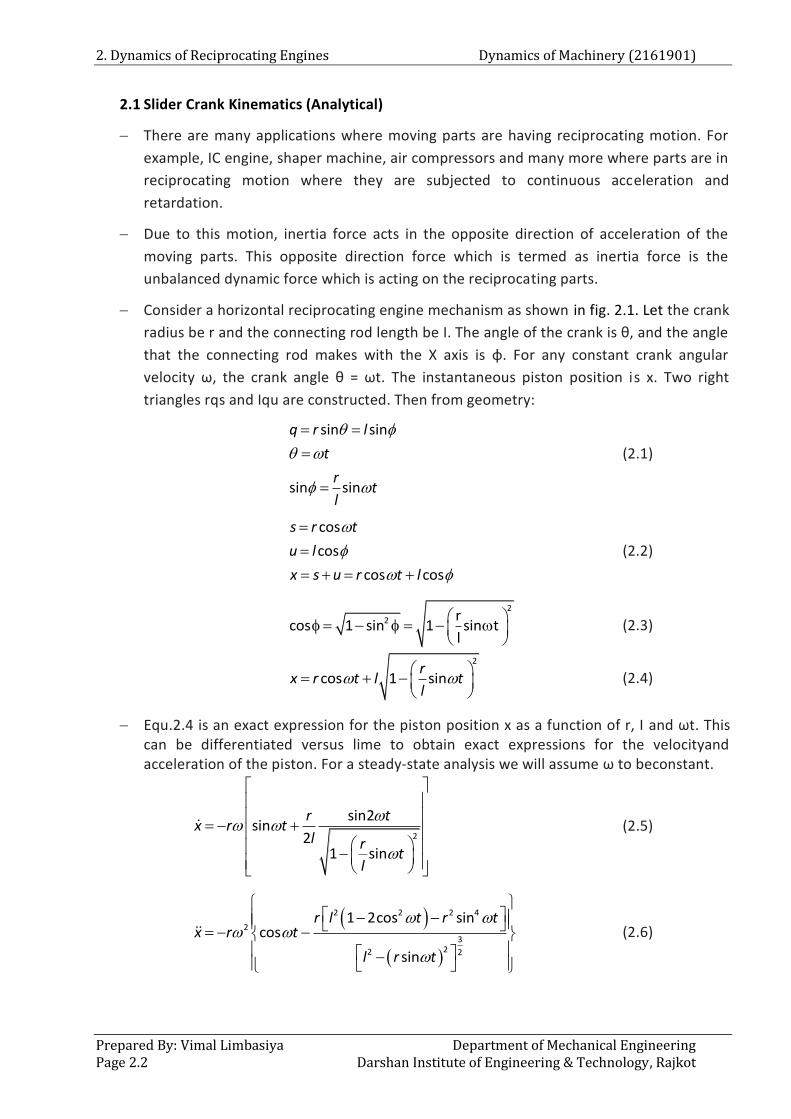
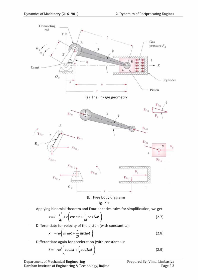
Consider a horizontal reciprocating engine mechanism as shown in fig. 2.1. Let the crank
radius be r and the connecting rod length be I. The angle of the crank is θ, and the angle
that the connecting rod makes with the X axis is φ. For any constant crank angular
velocity ω, the crank angle θ = ωt. The instantaneous piston position is x. Two right
triangles rqs and Iqu are constructed. Then from geometry:
sin sin
sin sin
q r l
t
rt
l
(2.1)
cos
cos
cos cos
s r t
u l
x s u r t l
(2.2)
2
2 rcos 1 sin 1 sin t
l
(2.3)
2
cos 1 sinr
x r t l tl
(2.4)
Equ.2.4 is an exact expression for the piston position x as a function of r, I and ωt. This can be differentiated versus lime to obtain exact expressions for the velocityand acceleration of the piston. For a steady-state analysis we will assume ω to beconstant.
2
sin2sin
21 sin
r tx r t
l rt
l
(2.5)
2 2 2 4
2
322 2
1 2cos sincos
sin
r l t r tx r t
l r t
(2.6)
Dynamics of Machinery (2161901) 2. Dynamics of Reciprocating Engines
Department of Mechanical Engineering Prepared By: Vimal Limbasiya Darshan Institute of Engineering & Technology, Rajkot Page 2.3
(a) The linkage geometry
(b) Free body diagrams
Fig. 2.1
Applying binomial theorem and Fourier series rules for simplification, we get 2
cos cos24 4
r rx l r t t
l l
(2.7)
Differentiate for velocity of the piston (with constant ω):
sin sin22
rx r t t
l
(2.8)
Differentiate again for acceleration (with constant ω):
2 cos cos2r
x r t tl
(2.9)
2. Dynamics of Reciprocating Engines Dynamics of Machinery (2161901)
Prepared By: Vimal Limbasiya Department of Mechanical Engineering Page 2.4 Darshan Institute of Engineering & Technology, Rajkot
2.2 Gas Force and Gas Torque
The gas force is due to the gas pressure from the exploding fuel-air mixture impinging
on the top of the piston surface as shown in Fig. 2.1(a). Let Fg = gas force. Pg = gas
pressure, Ap = area of piston and B = bore of cylinder, which is also equal to the piston
diameter. Then:
2
2
,4
4
g g p p
g g
F P A where A B
F P B
The negative sign is due to the choice of engine orientation in the coordinate system.
The gas pressure Pg in this expression is a function of crank angle ωt and is defined by
the thermodynamics of the engine.
The gas torque is due to the gas force acting at a moment arm about the crank center in
Fig. 2.1 This moment arm varies from zero to a maximum as the crank rotates.
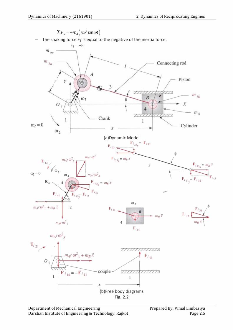
2.3 Inertia and Shaking Forces
The simplifiedlumped mass model of Fig. 2.2 can be used to develop expressions forthe
forces and torques due to the accelerations of the masses in the system.
The acceleration for point B is given in equation
2 cos cos2r
x r t tl
The accelerationof point A in pure rotation is obtained by differentiating the position
vector RAtwice, assuming a constant crankshaft ω. which gives:
RA = rcosωt + rsinωt (2.10)
aA = –rω2cosωt–rω2sinωt (2.11)
The total inertia force Fi is the sum of the centrifugal (inertia) force at point A andthe
inertia force at point B.
Fi = –mAaA –mBaB (2.12)
Breaking it into x and y components:
2 cosi x A BF m r t m x (2.13)
2 sini y AF m r t (2.14)
Note that only the x component is affected by the acceleration of the piston.
2 2
2
cos cos cos2
sin
i x A B
i y A
rF m r t m r t t
l
F m r t
The shaking force is defined asthe sum of all forcesacting on the ground plane. From the
free-body diagram for link 1 in Fig. 2.2
2 2cos cos cos2S x A B
rF m r t m r t t
l
Dynamics of Machinery (2161901) 2. Dynamics of Reciprocating Engines
Department of Mechanical Engineering Prepared By: Vimal Limbasiya Darshan Institute of Engineering & Technology, Rajkot Page 2.5
2 sini y AF m r t
The shaking force FS is equal to the negative of the inertia force. FS = –Fi
(a)Dynamic Model
(b)Free body diagrams
Fig. 2.2
2. Dynamics of Reciprocating Engines Dynamics of Machinery (2161901)
Prepared By: Vimal Limbasiya Department of Mechanical Engineering Page 2.6 Darshan Institute of Engineering & Technology, Rajkot
2.4 Inertia and Shaking Torques
The inertia torque results from the action of the inertia forces at a moment arm. The
inertia force at point A in Fig. 2.2 has two components, radial and tangential. The radial
component has no moment arm. The tangential component has a moment arm of crank
radius r.
If the crank ω is constant, the mass at A will not contribute to inertia torque. The inertia
force at B has a nonzero component perpendicular to the cylinder wall except when the
piston is at TDC or BDC.
As we did for the gas torque, we can express the inertia torque in terms of the couple –
Fi41, Fi41 whose forces act always perpendicular to the motion of the slider (neglecting
friction), and the distance x, which is their instantaneous moment arm. The inertia
torque is:
Ti21= Fi41.x = –Fi41.x
Substituting value of Fi41 and x, we get
2
21 tan cos cos24 4
i B
r rT m x l r t t
l l
The shaking torque is equal to the inertia torque.
Ts = Ti21.
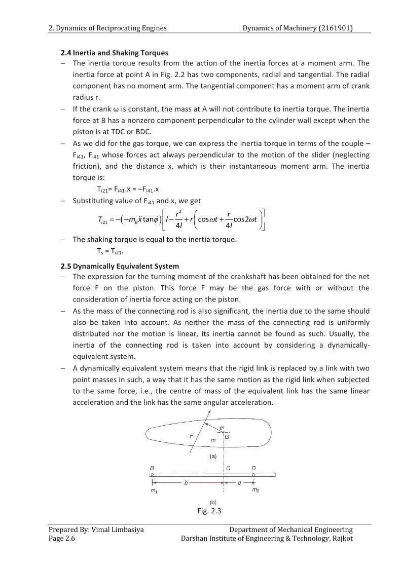
2.5 Dynamically Equivalent System
The expression for the turning moment of the crankshaft has been obtained for the net
force F on the piston. This force F may be the gas force with or without the
consideration of inertia force acting on the piston.
As the mass of the connecting rod is also significant, the inertia due to the same should
also be taken into account. As neither the mass of the connecting rod is uniformly
distributed nor the motion is linear, its inertia cannot be found as such. Usually, the
inertia of the connecting rod is taken into account by considering a dynamically-
equivalent system.
A dynamically equivalent system means that the rigid link is replaced by a link with two
point masses in such, a way that it has the same motion as the rigid link when subjected
to the same force, i.e., the centre of mass of the equivalent link has the same linear
acceleration and the link has the same angular acceleration.
Fig. 2.3
Dynamics of Machinery (2161901) 2. Dynamics of Reciprocating Engines
Department of Mechanical Engineering Prepared By: Vimal Limbasiya Darshan Institute of Engineering & Technology, Rajkot Page 2.7
Fig. 2.3(a) shows a rigid body of mass m with the centre of mass at G. Let it be acted
upon by a force F which produces linear acceleration a of the centre of mass as well as
angular acceleration of the body asthe force F does not pass through G.
As we know,
F = m.a and F.e = I. α
Acceleration of G,
Fa
m
Angular acceleration ofthe body,
.F e
I
where e = perpendicular distance ofF from G
and I = moment of inertia of the body about perpendicular axis through G
Now to have the dynamically equivalent system, let the replaced massless link [Fig.
2.3(b)] has two point masses m1 (at B and m2 at D) at distances b and d respectively
from the centre of mass G as shown in fig. 2.3(b).
1. To satisfy the first condition, as the force F is to be same, the sum of the equivalent
masses m1 and m2 has to be equal to mtohave the same acceleration. Thus, m = m1 +
m2.
2. To satisfy the second condition, the numerator F.e and the denominator I must remain
the same. F is already taken same, Thus, e has to be same which means that the
perpendicular distance of F from G should remain same or the combined centre of mass
of the equivalent system remains at G. This is Possible if
m1b = m2d
To have the same moment of inertia of the equivalent system about perpendicular axis
through their combined centre of mass G, we must have
I = m1b2+ m2d2
Thus, any distributed mass can be replaced by two point masses to have the same
dynamical properties if the following conditions are fulfilled:
(i) The sum of the two masses is equal to the total mass.
(ii) The combined centre of mass coincides with that of the rod.
(iii) The moment of inertia of two point masses about the perpendicular axis through
their combined centre of mass is equal to that of the rod.
2.6 Pin Forces in the Single Cylinder Engine In addition to calculating the overall effects on the ground plane of the dynamic
forcespresent in the engine, we also need to know the magnitudes of the forces at the
pin joints.
These forces will dictate the design of the pins and the bearings at thejoints. Though
wewere able to lump the mass due to both connecting rod and piston, or connecting rod
and crank at pointsA and B for an overall analysis of the linkage's effects on the ground
plane, we cannot doso for the pin force calculations.
2. Dynamics of Reciprocating Engines Dynamics of Machinery (2161901)
Prepared By: Vimal Limbasiya Department of Mechanical Engineering Page 2.8 Darshan Institute of Engineering & Technology, Rajkot
This is because the pins feel the effect of the connecting rodpulling on one "side" and
the piston (or crank) pulling on the other "side" of the pin. Thus we must separate the
effects of the masses of thelinks joined by the pins.
We will calculate the effect of each component due to the various masses, and the gas
force and then superpose them to obtain the complete pin force at each joint. The
resultant bearing loads have the following components:
i. The gas force components.
ii. The inertia force due to the piston mass.
iii. The inertia force due to the mass of the connecting rod at the wrist pin.
iv. The inertia force due to the mass of the connecting rod at the crank pin.
v. The inertia force due to the mass of the crank at the crank pin.
2.7 Balancing of unbalanced forces in reciprocating masses
Acceleration of reciprocating mass of a slider-crank mechanism is given by 2 cos2
cosa rn
Therefore, the force required to accelerate mass m is
2 cos2cosF mr
n
2 2 cos2cosF mr mr
n
mrω2cosθ is called the primary accelerating force and mrω2 cos2θ/n is called the
secondary accelerating force.
Maximum value of the primary force = mrω2
Maximum value of the secondary force =mrω2/n
As n is, usually, much greater than unity, the secondary force is small, compared with
the primary force and can be safely neglected for slow-speed engines.
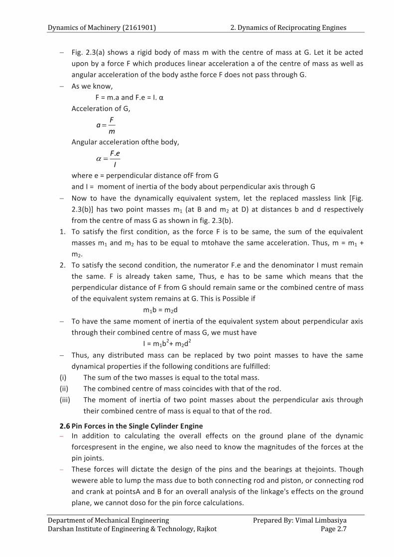
The inertia force due to primary accelerating force is shown in Fig. 2.4(a). In Fig. 2.4(b),
the forces acting on the engine frame due to this inertia force are shown. The force
exerted by the crankshaft on the main bearings has two components, F21h and F21v.
The horizontal force F21h is an unbalanced shaking force. The vertical forces F21v and
F41v balance each other, but form an unbalanced shaking couple. The magnitude and
direction of this force and couple go on changing with the rotation of the crank angle θ.
The shaking force produces linear vibration of the frame in the horizontal direction
whereas the shaking couple produces an oscillating vibration.
Thus, it is seen that the shaking force F21h is the only unbalanced force. It may hamper
the smooth running of the engine and Thus, effort is made to balance the same.
However, it is not at all possible to balance it completely and only some modification
can be made.
Dynamics of Machinery (2161901) 2. Dynamics of Reciprocating Engines
Department of Mechanical Engineering Prepared By: Vimal Limbasiya Darshan Institute of Engineering & Technology, Rajkot Page 2.9
Fig. 2.4
The usual approach of balancing the shaking force is by addition of a rotating
countermass at radius r directly opposite the crank which however, provides only a
partial balance. This countermass is in addition to the mass used to balance the rotating
unbalance due to the mass at the crank pin.
Fig. 2.4(c) shows the reciprocating mechanism with a countermass m at the radial
distance r. The horizontal component of the centrifugal force due to the balancing mass
is mrω2cosθ in the line of stroke.
This neutralizes the unbalanced reciprocating force. But the rotating mass also has a
component mrω2sinθ perpendicular to the line of stroke which remains unbalanced.
The unbalanced force is zero at the ends of the stroke when 0 = 0° or 180° and
maximum at the middle when θ = 90°.
The magnitude or the maximum value of the unbalanced force remains the same, i.e.,
equal to mrω2. Thus, instead of sliding to and fro on its mounting, the mechanism tends
to jump up and down.
2. Dynamics of Reciprocating Engines Dynamics of Machinery (2161901)
Prepared By: Vimal Limbasiya Department of Mechanical Engineering Page 2.10 Darshan Institute of Engineering & Technology, Rajkot
To minimize the effect of the unbalanced force, a compromise is, usually, made, i.e., 2/3
of the reciprocating mass is balanced (or a value between one-half and three-quarters).
If c is the fraction of the reciprocating mass Thus, balanced then
primary force balanced by the mass = cmrω2cosθ
primary force unbalanced by the mass = (1 -c)mrω2cosθ
Vertical component of centrifugal force whichremains unbalanced
= cmrω2sinθ
In fact, in reciprocating engines, unbalanced forces in the direction of the line of
stroke are more dangerous than the forces perpendicular to the line of stroke.
Resultant unbalanced force at any instant
2 22 2(1 ) cos sinc mr cmr
The resultant unbalanced force is minimum when c = 1/2.
The method just discussed above to balance the disturbing effect of a reciprocating
mass is just equivalent to as if a revolving mass at the crankpin is completely
balanced by providing a countermass at the same radius diametrically opposite the
crank.
Thus, if mp is the mass at the crankpin and c is the fraction of the reciprocating mass
m to be balanced, the mass at the crankpin may be considered as (cm + mp) which
is to be completely balanced.
Example 2.1: The following data relate to a single - cylinder reciprocating engine:
Mass of reciprocating parts = 40 kg
Mass of revolving parts = 30 kg at crank radius
Speed = 150 rpm
Stroke = 350 mm
If 60% of the reciprocating parts and all the revolving parts are to be balanced, determine (i)
balance mass required at a radius of 320 mm
(ii) unbalanced force when the crank has turned 45° from top dead centre.
m = 40 kg
mP = 30 kg
N = 150 rpm
r = l/2 =175 mm
2 2 150
60 60
15.7 /
N
rad s
(i) Mass to be balanced at crank pin = cm + mP
= 0.6 x 40 +30
= 54 kg
Dynamics of Machinery (2161901) 2. Dynamics of Reciprocating Engines
Department of Mechanical Engineering Prepared By: Vimal Limbasiya Darshan Institute of Engineering & Technology, Rajkot Page 2.11
mCrC = mr
mC x 320 = 54 x 175
mC = 29.53 kg.
(ii) Unbalanced force (at θ = 45°)
2 22 2(1 ) cos sinc mr cmr
2 22 2(1 0.6) 40 0.175 (15.7) cos45 0.6 40 0.175 (15.7) sin45
= 880.1 N.
Example 2.2:A single cylinder reciprocating engine has speed 240 rpm, stroke 300 mm, mass of
reciprocating parts 50 kg, mass of revolving parts at 150 mm radius 30 kg. If all the mass of
revolving parts and two-third of the mass of reciprocating parts are to be balanced, find the
balance mass required at radius of 400 mm and the residual unbalanced force when the crank
has rotated 60 from IDC.
N = 240 rpm
l = 300 mm
m = 50 kg
mP = 30 kg
r = l/2 =150 mm
2 2 240
60 60
25.13 /
N
rad s
(i) Mass to be balanced at crank pin = cm + mP
= 2/3 x 50 + 30
= 63.33 kg
mCrC = mr
mC x 400 = 63.33 x 150
mC = 23.75 kg.
(ii) Unbalanced force (at θ = 45°)
2 22 2(1 ) cos sinc mr cmr
2 2
2 22 2(1 ) 50 0.15 (25.13) cos60 50 0.15 (25.13) sin60
3 3
2 2(789.36) (2734.55)
= 2846.2 N
2. Dynamics of Reciprocating Engines Dynamics of Machinery (2161901)
Prepared By: Vimal Limbasiya Department of Mechanical Engineering Page 2.12 Darshan Institute of Engineering & Technology, Rajkot
2.8 Balancing of Locomotives
Locomotives are of two types, coupled and uncoupled. If two or more pairs of wheels are
coupled together to increase the adhesive force between the wheels and the track, it is
called a coupled locomotive. Otherwise, it is an uncoupled locomotive.
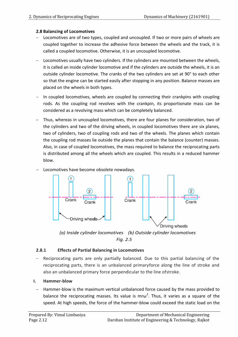
Locomotives usually have two cylinders. If the cylinders are mounted between the wheels,
it is called an inside cylinder locomotive and if the cylinders are outside the wheels, it is an
outside cylinder locomotive. The cranks of the two cylinders are set at 90° to each other
so that the engine can be started easily after stopping in any position. Balance masses are
placed on the wheels in both types.
In coupled locomotives, wheels are coupled by connecting their crankpins with coupling
rods. As the coupling rod revolves with the crankpin, its proportionate mass can be
considered as a revolving mass which can be completely balanced.
Thus, whereas in uncoupled locomotives, there are four planes for consideration, two of
the cylinders and two of the driving wheels, in coupled locomotives there are six planes,
two of cylinders, two of coupling rods and two of the wheels. The planes which contain
the coupling rod masses lie outside the planes that contain the balance (counter) masses.
Also, in case of coupled locomotives, the mass required to balance the reciprocating parts
is distributed among all the wheels which are coupled. This results in a reduced hammer
blow.
Locomotives have become obsolete nowadays.
(a) Inside cylinder locomotives (b) Outside cylinder locomotives
Fig. 2.5
2.8.1 Effects of Partial Balancing in Locomotives
Reciprocating parts are only partially balanced. Due to this partial balancing of the
reciprocating parts, there is an unbalanced primaryforce along the line of stroke and
also an unbalanced primary force perpendicular to the line ofstroke.
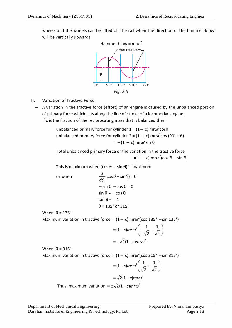
I. Hammer-blow
Hammer-blow is the maximum vertical unbalanced force caused by the mass provided to
balance the reciprocating masses. Its value is mrω2. Thus, it varies as a square of the
speed. At high speeds, the force of the hammer-blow could exceed the static load on the
Dynamics of Machinery (2161901) 2. Dynamics of Reciprocating Engines
Department of Mechanical Engineering Prepared By: Vimal Limbasiya Darshan Institute of Engineering & Technology, Rajkot Page 2.13
wheels and the wheels can be lifted off the rail when the direction of the hammer-blow
will be vertically upwards.
Hammer blow = mrω2
Fig. 2.6
II. Variation of Tractive Force
A variation in the tractive force (effort) of an engine is caused by the unbalanced portion
of primary force which acts along the line of stroke of a locomotive engine.
If c is the fraction of the reciprocating mass that is balanced then
unbalanced primary force for cylinder 1 = (1 c) mrω2cosθ
unbalanced primary force for cylinder 2 = (1 c) mrω2cos (90° + θ)
= (1 c) mrω2sin θ
Total unbalanced primary force or the variation in the tractive force
= (1 c) mrω2(cos θ sin θ)
This is maximum when (cos θ sin θ) is maximum,
or when (cos sin ) 0d
d
sin θ cos θ = 0
sin θ = cos θ
tan θ = 1
θ = 135° or 315°
When θ = 135°
Maximum variation in tractive force = (1 c) mrω2(cos 135° sin 135°)
2 1 1(1 )
2 2c mr
22(1 )c mr
When θ = 315°
Maximum variation in tractive force = (1 c) mrω2(cos 315° sin 315°)
2 1 1(1 )
2 2c mr
22(1 )c mr
Thus, maximum variation 22(1 )c mr
2. Dynamics of Reciprocating Engines Dynamics of Machinery (2161901)
Prepared By: Vimal Limbasiya Department of Mechanical Engineering Page 2.14 Darshan Institute of Engineering & Technology, Rajkot
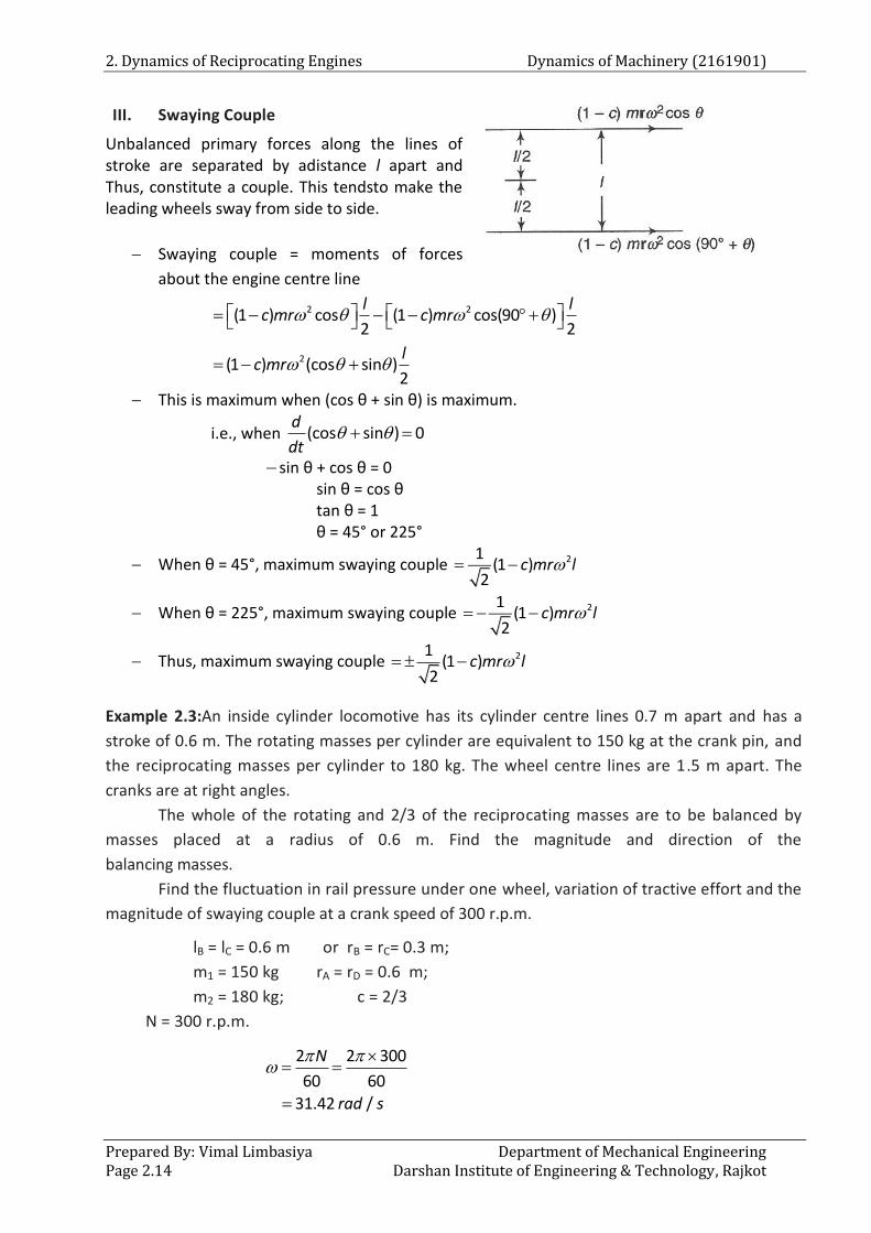
III. Swaying Couple
Unbalanced primary forces along the lines of stroke are separated by adistance l apart and Thus, constitute a couple. This tendsto make the leading wheels sway from side to side.
Swaying couple = moments of forces
about the engine centre line
2 2(1 ) cos (1 ) cos(90 )2 2
l lc mr c mr
2(1 ) (cos sin )2
lc mr
This is maximum when (cos θ + sin θ) is maximum.
i.e., when (cos sin ) 0d
dt
sin θ + cos θ = 0 sin θ = cos θ tan θ = 1
θ = 45° or 225°
When θ = 45°, maximum swaying couple 21(1 )
2c mr l
When θ = 225°, maximum swaying couple 21(1 )
2c mr l
Thus, maximum swaying couple 21(1 )
2c mr l
Example 2.3:An inside cylinder locomotive has its cylinder centre lines 0.7 m apart and has a
stroke of 0.6 m. The rotating masses per cylinder are equivalent to 150 kg at the crank pin, and
the reciprocating masses per cylinder to 180 kg. The wheel centre lines are 1.5 m apart. The
cranks are at right angles.
The whole of the rotating and 2/3 of the reciprocating masses are to be balanced by
masses placed at a radius of 0.6 m. Find the magnitude and direction of the
balancing masses.
Find the fluctuation in rail pressure under one wheel, variation of tractive effort and the
magnitude of swaying couple at a crank speed of 300 r.p.m.
lB = lC = 0.6 m or rB = rC= 0.3 m;
m1 = 150 kg rA = rD = 0.6 m;
m2 = 180 kg; c = 2/3
N = 300 r.p.m.
2 2 300
60 60
31.42 /
N
rad s
Dynamics of Machinery (2161901) 2. Dynamics of Reciprocating Engines
Department of Mechanical Engineering Prepared By: Vimal Limbasiya Darshan Institute of Engineering & Technology, Rajkot Page 2.15
Equivalent mass of the rotating parts to be balanced per cylinder at the crank pin,
m = mB = mC = m1 + c.m2
2150 180
3 = 270 kg
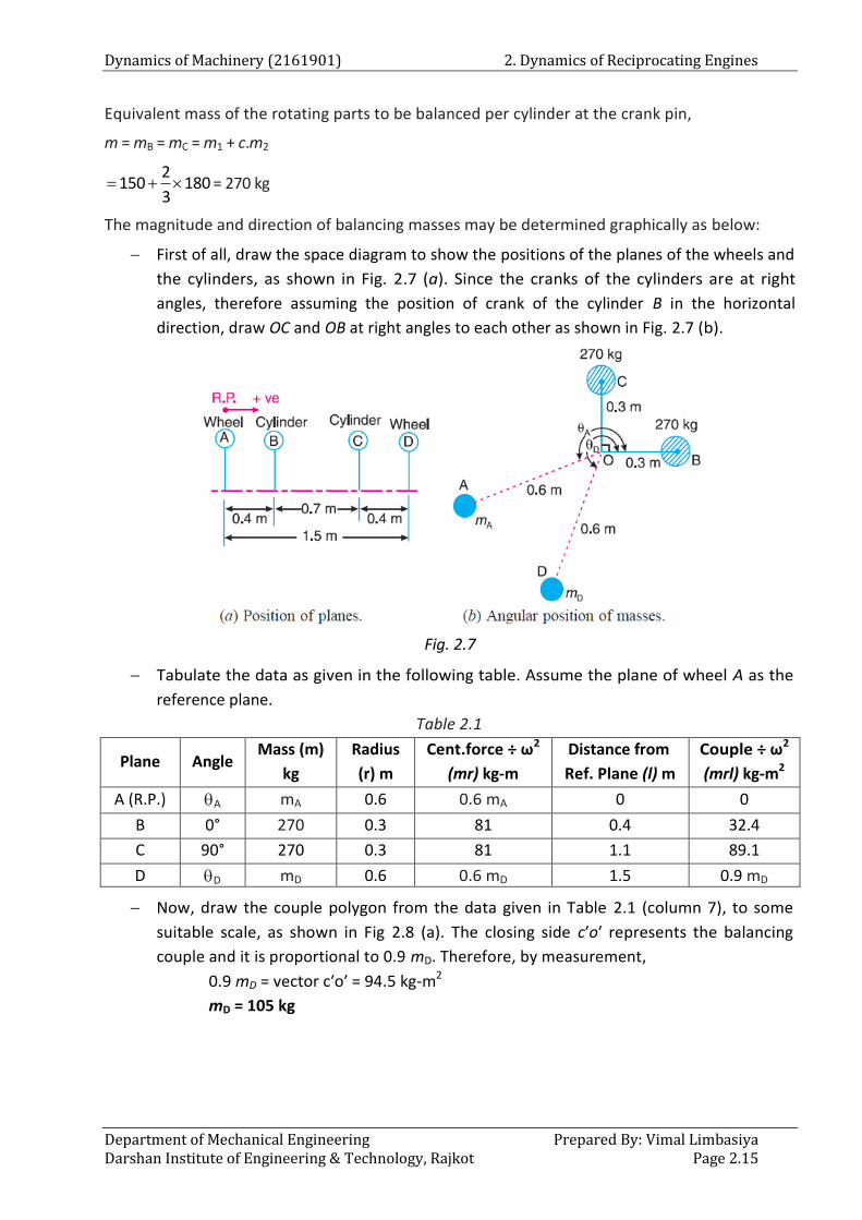
The magnitude and direction of balancing masses may be determined graphically as below:
First of all, draw the space diagram to show the positions of the planes of the wheels and
the cylinders, as shown in Fig. 2.7 (a). Since the cranks of the cylinders are at right
angles, therefore assuming the position of crank of the cylinder B in the horizontal
direction, draw OC and OB at right angles to each other as shown in Fig. 2.7 (b).
Fig. 2.7
Tabulate the data as given in the following table. Assume the plane of wheel A as the
reference plane.
Table 2.1
Plane Angle Mass (m)
kg
Radius
(r) m
Cent.force ÷ ω2
(mr) kg-m
Distance from
Ref. Plane (l) m
Couple ÷ ω2
(mrl) kg-m2
A (R.P.) A mA 0.6 0.6 mA 0 0
B 0° 270 0.3 81 0.4 32.4
C 90° 270 0.3 81 1.1 89.1
D D mD 0.6 0.6 mD 1.5 0.9 mD
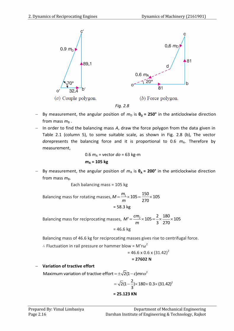
Now, draw the couple polygon from the data given in Table 2.1 (column 7), to some
suitable scale, as shown in Fig 2.8 (a). The closing side c′o′ represents the balancing
couple and it is proportional to 0.9 mD. Therefore, by measurement,
0.9 mD = vector c′o′ = 94.5 kg-m2
mD = 105 kg
2. Dynamics of Reciprocating Engines Dynamics of Machinery (2161901)
Prepared By: Vimal Limbasiya Department of Mechanical Engineering Page 2.16 Darshan Institute of Engineering & Technology, Rajkot
Fig. 2.8
By measurement, the angular position of mD is θD = 250° in the anticlockwise direction
from mass mB .
In order to find the balancing mass A, draw the force polygon from the data given in
Table 2.1 (column 5), to some suitable scale, as shown in Fig. 2.8 (b), The vector
dorepresents the balancing force and it is proportional to 0.6 mA. Therefore by
measurement,
0.6 mA = vector do = 63 kg-m
mA = 105 kg
By measurement, the angular position of mA is θA = 200° in the anticlockwise direction
from mass mB.
Each balancing mass = 105 kg
Balancing mass for rotating masses, 1 150105 105
270
mM
m
= 58.3 kg
Balancing mass for reciprocating masses, 2 2 180' 105 105
3 270
cmM
m
= 46.6 kg
Balancing mass of 46.6 kg for reciprocating masses gives rise to centrifugal force.
∴ Fluctuation in rail pressure or hammer blow = M’rω2
= 46.6 x 0.6 x (31.42)2
= 27602 N
Variation of tractive effort 2Maximum variation of tractive effort 2(1 )c mr
222(1 ) 180 0.3 (31.42)
3
= 25.123 KN
Dynamics of Machinery (2161901) 2. Dynamics of Reciprocating Engines
Department of Mechanical Engineering Prepared By: Vimal Limbasiya Darshan Institute of Engineering & Technology, Rajkot Page 2.17
Swaying couple
21Maximum swaying couple (1 )
2c mr l
21 2(1 ) 180 0.3 (31.42) 0.7
32
= 8797 N.m
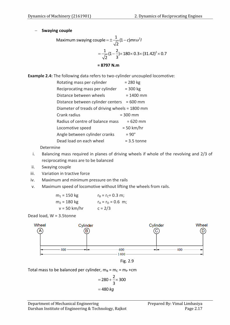
Example 2.4: The following data refers to two-cylinder uncoupled locomotive:
Rotating mass per cylinder = 280 kg
Reciprocating mass per cylinder = 300 kg
Distance between wheels = 1400 mm
Distance between cylinder centers = 600 mm
Diameter of treads of driving wheels = 1800 mm
Crank radius = 300 mm
Radius of centre of balance mass = 620 mm
Locomotive speed = 50 km/hr
Angle between cylinder cranks = 90°
Dead load on each wheel = 3.5 tonne
Determine
i. Balancing mass required in planes of driving wheels if whole of the revolving and 2/3 of
reciprocating mass are to be balanced
ii. Swaying couple
iii. Variation in tractive force
iv. Maximum and minimum pressure on the rails
v. Maximum speed of locomotive without lifting the wheels from rails.
m1 = 150 kg rB = rC= 0.3 m;
m2 = 180 kg rA = rD = 0.6 m;
v = 50 km/hr c = 2/3
Dead load, W = 3.5tonne
Fig. 2.9
Total mass to be balanced per cylinder, mB = mC = mP +cm
2280 300
3
480 kg
2. Dynamics of Reciprocating Engines Dynamics of Machinery (2161901)
Prepared By: Vimal Limbasiya Department of Mechanical Engineering Page 2.18 Darshan Institute of Engineering & Technology, Rajkot
Table 2.2
Plane Angle Mass (m)
kg
Radius
(r) m
Cent.force ÷ ω2
(mr) kg-m
Distance from
Ref. Plane (l) m
Couple ÷ ω2
(mrl) kg-m2
A (R.P.) A mA 0.62 0.62mA 0 0
B 0° 480 0.3 144 0.4 57.6
C 90° 480 0.3 144 1 144
D D mD 0.62 0.62mD 1.4 0.868mD
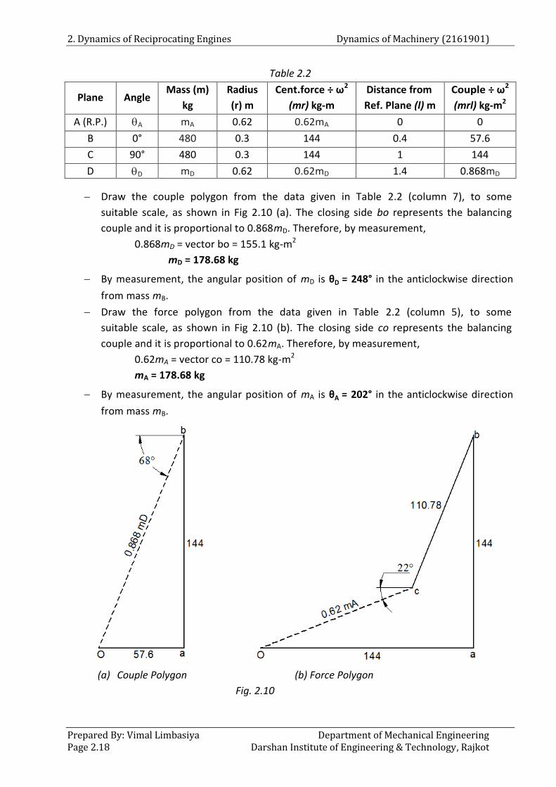
Draw the couple polygon from the data given in Table 2.2 (column 7), to some
suitable scale, as shown in Fig 2.10 (a). The closing side bo represents the balancing
couple and it is proportional to 0.868mD. Therefore, by measurement,
0.868mD = vector bo = 155.1 kg-m2
mD = 178.68 kg
By measurement, the angular position of mD is θD = 248° in the anticlockwise direction
from mass mB.
Draw the force polygon from the data given in Table 2.2 (column 5), to some
suitable scale, as shown in Fig 2.10 (b). The closing side co represents the balancing
couple and it is proportional to 0.62mA. Therefore, by measurement,
0.62mA = vector co = 110.78 kg-m2
mA = 178.68 kg
By measurement, the angular position of mA is θA = 202° in the anticlockwise direction
from mass mB.
(a) Couple Polygon (b) Force Polygon
Fig. 2.10
Dynamics of Machinery (2161901) 2. Dynamics of Reciprocating Engines
Department of Mechanical Engineering Prepared By: Vimal Limbasiya Darshan Institute of Engineering & Technology, Rajkot Page 2.19
v = rω
650 10 1
60 60 1800 / 2
v
r
= 15.43 rad/s
21Swaying couple (1 )
2c mr l
21 2(1 ) 300 0.3 (15.43) 0.6
32
= 3030.3 N.m
2Variation of tractive effort 2(1 )c mr
222(1 ) 300 0.3 (15.43)
3
= 10100 N
Balance mass for reciprocating parts only
2300
3178.7 74.46480
kg
Hammer blow = mrω2
= 74.46 x 0.62 x (15.43)2 = 10991 N
Dead load = 3.5 x 1000 x 9.81
= 34335 N
Maximum pressure on rails = 34335 + 10991
= 45326 N
Minimum pressure on rails = 34335 – 10991
= 23344 N
Maximum speed of the locomotive without lifting the wheels from the rails will be when the dead
load becomes equal to the hammer blow
74.46 x 0.62 x ω2 = 34335
ω = 27.27 rad/s
Velocity of wheels = rω
1.827.27 /
2m s
1.8 60 6027.27 /
2 1000km hr
V = 88.36 km / hr
2. Dynamics of Reciprocating Engines Dynamics of Machinery (2161901)
Prepared By: Vimal Limbasiya Department of Mechanical Engineering Page 2.20 Darshan Institute of Engineering & Technology, Rajkot
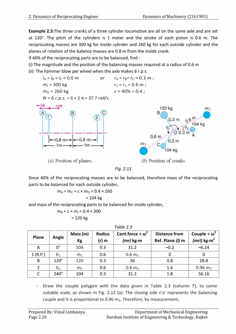
Example 2.5:The three cranks of a three cylinder locomotive are all on the same axle and are set
at 120°. The pitch of the cylinders is 1 meter and the stroke of each piston is 0.6 m. The
reciprocating masses are 300 kg for inside cylinder and 260 kg for each outside cylinder and the
planes of rotation of the balance masses are 0.8 m from the inside crank.
If 40% of the reciprocating parts are to be balanced, find :
(i) The magnitude and the position of the balancing masses required at a radius of 0.6 m
(ii) The hammer blow per wheel when the axle makes 6 r.p.s.
lA = lB = lC = 0.6 m or rA = rB= rC = 0.3 m ;
mI = 300 kg r1 = r2 = 0.6 m ;
mO = 260 kg c = 40% = 0.4 ;
N = 6 r.p.s. = 6 × 2 π = 37.7 rad/s
Fig. 2.11
Since 40% of the reciprocating masses are to be balanced, therefore mass of the reciprocating
parts to be balanced for each outside cylinder,
mA = mC = c × mO = 0.4 × 260
= 104 kg
and mass of the reciprocating parts to be balanced for inside cylinder,
mB = c × mI = 0.4 × 300
= 120 kg
Table 2.3
Plane Angle Mass (m)
Kg
Radius
(r) m
Cent.force ÷ ω2
(mr) kg-m
Distance from
Ref. Plane (l) m
Couple ÷ ω2
(mrl) kg-m2
A 0° 104 0.3 31.2 –0.2 –6.24
1 (R.P.) 1 m1 0.6 0.6 m1 0 0
B 120° 120 0.3 36 0.8 28.8
2 2 m2 0.6 0.6 m2 1.6 0.96 m2
C 240° 104 0.3 31.2 1.8 56.16
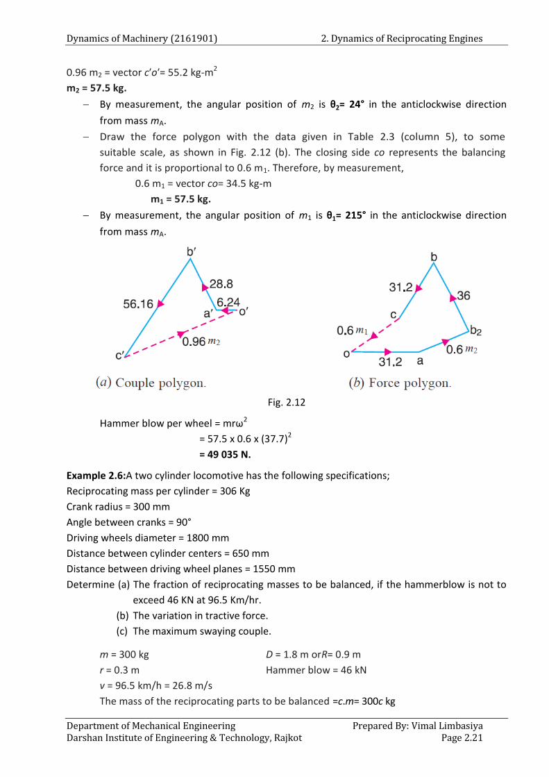
Draw the couple polygon with the data given in Table 2.3 (column 7), to some
suitable scale, as shown in Fig. 2.12 (a). The closing side c′o′ represents the balancing
couple and it is proportional to 0.96 m2. Therefore, by measurement,
Dynamics of Machinery (2161901) 2. Dynamics of Reciprocating Engines
Department of Mechanical Engineering Prepared By: Vimal Limbasiya Darshan Institute of Engineering & Technology, Rajkot Page 2.21
0.96 m2 = vector c′o′= 55.2 kg-m2
m2 = 57.5 kg.
By measurement, the angular position of m2 is θ2= 24° in the anticlockwise direction
from mass mA.
Draw the force polygon with the data given in Table 2.3 (column 5), to some
suitable scale, as shown in Fig. 2.12 (b). The closing side co represents the balancing
force and it is proportional to 0.6 m1. Therefore, by measurement,
0.6 m1 = vector co= 34.5 kg-m
m1 = 57.5 kg.
By measurement, the angular position of m1 is θ1= 215° in the anticlockwise direction
from mass mA.
Fig. 2.12
Hammer blow per wheel = mrω2
= 57.5 x 0.6 x (37.7)2
= 49 035 N.
Example 2.6:A two cylinder locomotive has the following specifications;
Reciprocating mass per cylinder = 306 Kg
Crank radius = 300 mm
Angle between cranks = 90°
Driving wheels diameter = 1800 mm
Distance between cylinder centers = 650 mm
Distance between driving wheel planes = 1550 mm
Determine (a) The fraction of reciprocating masses to be balanced, if the hammerblow is not to
exceed 46 KN at 96.5 Km/hr.
(b) The variation in tractive force.
(c) The maximum swaying couple.
m = 300 kg D = 1.8 m orR= 0.9 m
r = 0.3 m Hammer blow = 46 kN
v = 96.5 km/h = 26.8 m/s
The mass of the reciprocating parts to be balanced =c.m= 300c kg
2. Dynamics of Reciprocating Engines Dynamics of Machinery (2161901)
Prepared By: Vimal Limbasiya Department of Mechanical Engineering Page 2.22 Darshan Institute of Engineering & Technology, Rajkot
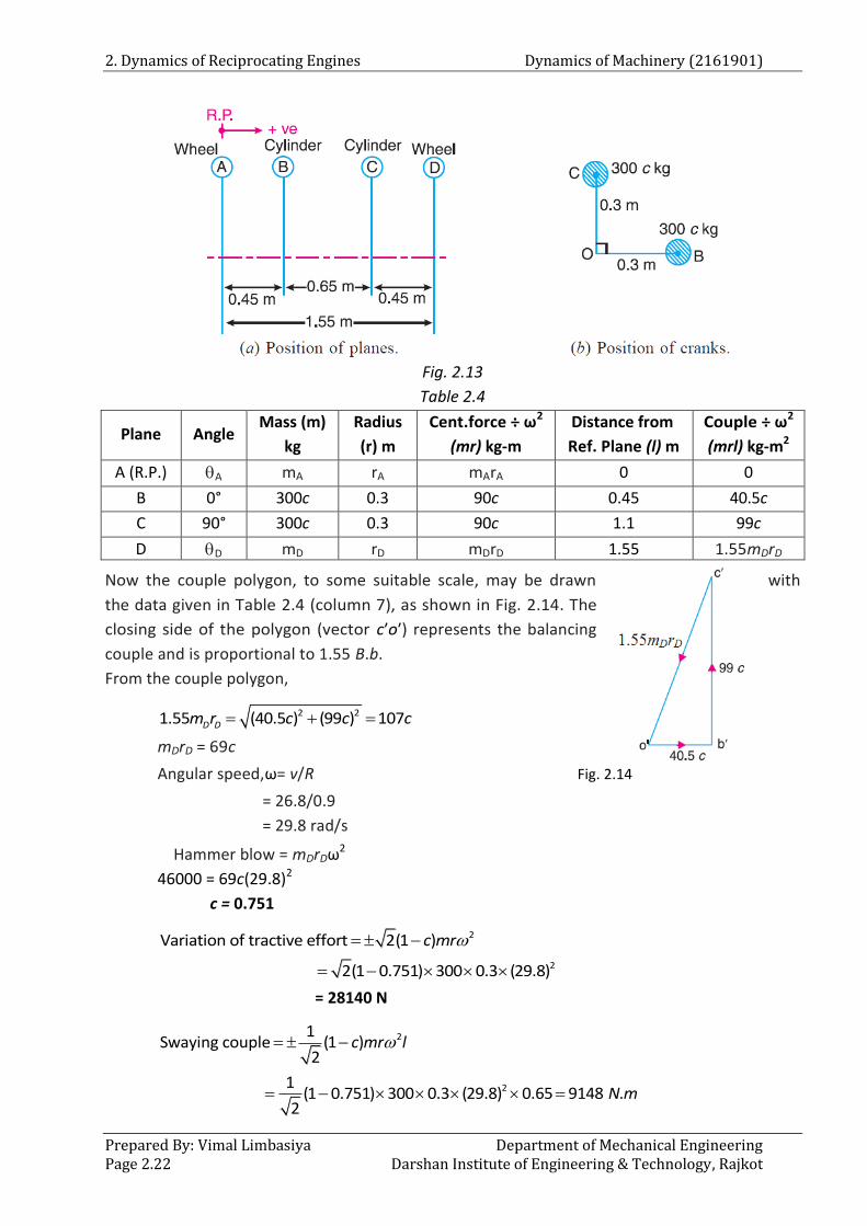
Fig. 2.13
Table 2.4
Plane Angle Mass (m)
kg
Radius
(r) m
Cent.force ÷ ω2
(mr) kg-m
Distance from
Ref. Plane (l) m
Couple ÷ ω2
(mrl) kg-m2
A (R.P.) A mA rA mArA 0 0
B 0° 300c 0.3 90c 0.45 40.5c
C 90° 300c 0.3 90c 1.1 99c
D D mD rD mDrD 1.55 1.55mDrD
Now the couple polygon, to some suitable scale, may be drawn with
the data given in Table 2.4 (column 7), as shown in Fig. 2.14. The
closing side of the polygon (vector c′o′) represents the balancing
couple and is proportional to 1.55 B.b.
From the couple polygon,
2 21.55 (40.5 ) (99 ) 107D Dm r c c c
mDrD = 69c
Angular speed,ω= v/R Fig. 2.14
= 26.8/0.9
= 29.8 rad/s
Hammer blow = mDrDω2
46000 = 69c(29.8)2
c = 0.751
2Variation of tractive effort 2(1 )c mr
22(1 0.751) 300 0.3 (29.8) = 28140 N
21Swaying couple (1 )
2c mr l
21(1 0.751) 300 0.3 (29.8) 0.65 9148 .
2N m
Dynamics of Machinery (2161901) 2. Dynamics of Reciprocating Engines
Department of Mechanical Engineering Prepared By: Vimal Limbasiya Darshan Institute of Engineering & Technology, Rajkot Page 2.23
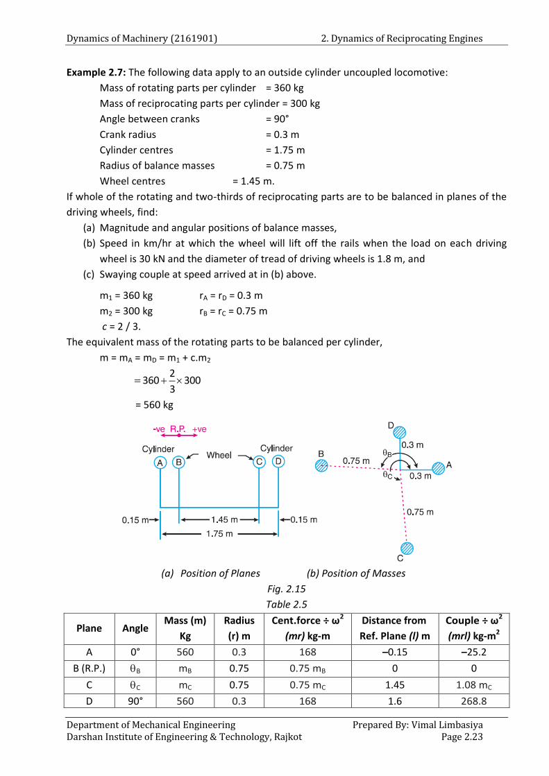
Example 2.7: The following data apply to an outside cylinder uncoupled locomotive:
Mass of rotating parts per cylinder = 360 kg
Mass of reciprocating parts per cylinder = 300 kg
Angle between cranks = 90°
Crank radius = 0.3 m
Cylinder centres = 1.75 m
Radius of balance masses = 0.75 m
Wheel centres = 1.45 m.
If whole of the rotating and two-thirds of reciprocating parts are to be balanced in planes of the
driving wheels, find:
(a) Magnitude and angular positions of balance masses,
(b) Speed in km/hr at which the wheel will lift off the rails when the load on each driving
wheel is 30 kN and the diameter of tread of driving wheels is 1.8 m, and
(c) Swaying couple at speed arrived at in (b) above.
m1 = 360 kg rA = rD = 0.3 m
m2 = 300 kg rB = rC = 0.75 m
c = 2 / 3.
The equivalent mass of the rotating parts to be balanced per cylinder,
m = mA = mD = m1 + c.m2
2360 300
3
= 560 kg
(a) Position of Planes (b) Position of Masses
Fig. 2.15
Table 2.5
Plane Angle Mass (m)
Kg
Radius
(r) m
Cent.force ÷ ω2
(mr) kg-m
Distance from
Ref. Plane (l) m
Couple ÷ ω2
(mrl) kg-m2
A 0° 560 0.3 168 –0.15 –25.2
B (R.P.) B mB 0.75 0.75 mB 0 0
C C mC 0.75 0.75 mC 1.45 1.08 mC
D 90° 560 0.3 168 1.6 268.8
2. Dynamics of Reciprocating Engines Dynamics of Machinery (2161901)
Prepared By: Vimal Limbasiya Department of Mechanical Engineering Page 2.24 Darshan Institute of Engineering & Technology, Rajkot
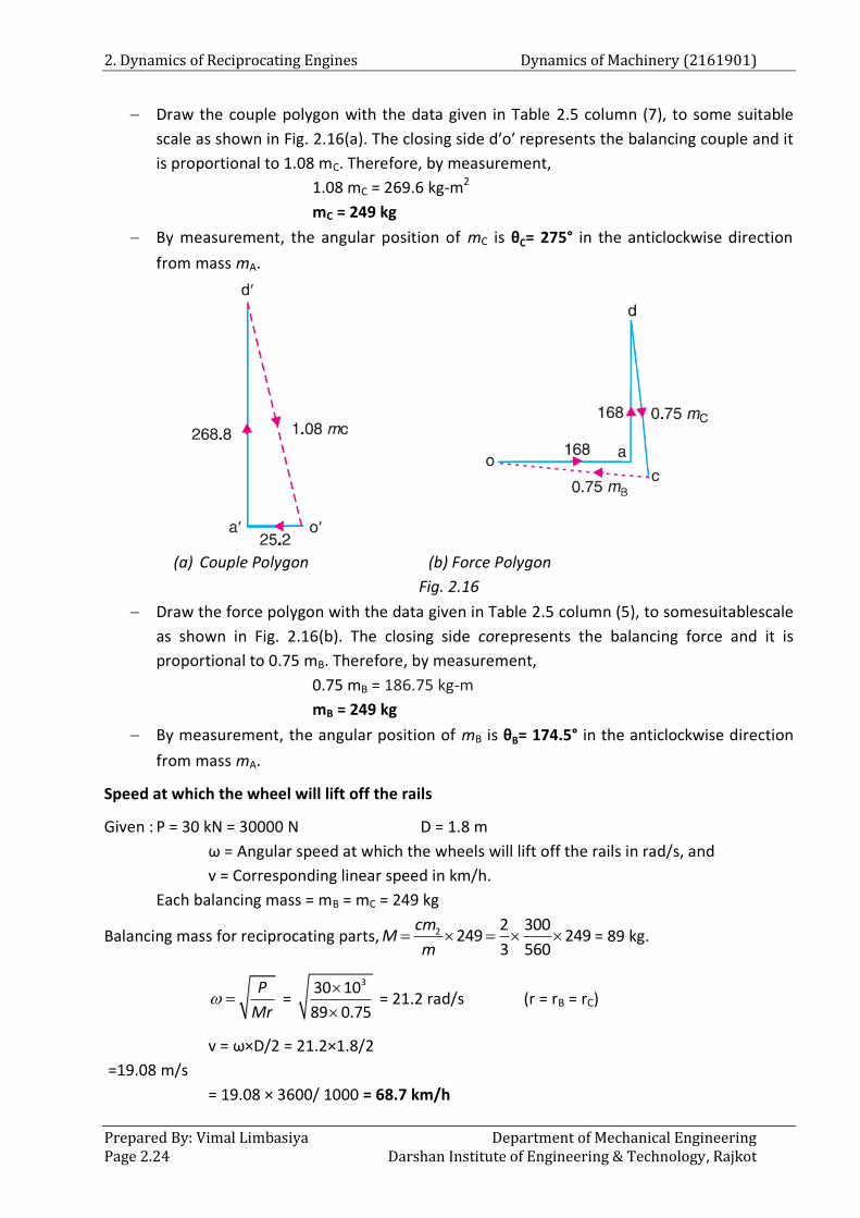
Draw the couple polygon with the data given in Table 2.5 column (7), to some suitable
scale as shown in Fig. 2.16(a). The closing side d′o′ represents the balancing couple and it
is proportional to 1.08 mC. Therefore, by measurement,
1.08 mC = 269.6 kg-m2
mC = 249 kg
By measurement, the angular position of mC is θC= 275° in the anticlockwise direction
from mass mA.
(a) Couple Polygon (b) Force Polygon
Fig. 2.16
Draw the force polygon with the data given in Table 2.5 column (5), to somesuitablescale
as shown in Fig. 2.16(b). The closing side corepresents the balancing force and it is
proportional to 0.75 mB. Therefore, by measurement,
0.75 mB = 186.75 kg-m
mB = 249 kg
By measurement, the angular position of mB is θB= 174.5° in the anticlockwise direction
from mass mA.
Speed at which the wheel will lift off the rails
Given : P = 30 kN = 30000 N D = 1.8 m
ω = Angular speed at which the wheels will lift off the rails in rad/s, and
v = Corresponding linear speed in km/h.
Each balancing mass = mB = mC = 249 kg
Balancing mass for reciprocating parts, 2 2 300249 249
3 560
cmM
m = 89 kg.
P
Mr =
330 10
89 0.75
= 21.2 rad/s (r = rB = rC)
v = ω×D/2 = 21.2×1.8/2
=19.08 m/s
= 19.08 × 3600/ 1000 = 68.7 km/h
Dynamics of Machinery (2161901) 2. Dynamics of Reciprocating Engines
Department of Mechanical Engineering Prepared By: Vimal Limbasiya Darshan Institute of Engineering & Technology, Rajkot Page 2.25
Swaying couple at speed ω = 21.1 rad/s
22
1Swaying couple (1 )
2c m r l
21 2(1 ) 300 0.3 (21.2) 1.75
32
= 16687 N.m
Example 2.8: The following data refers to a four-coupled wheel locomotive with two inside
cylinder
Pitch of cylinders = 600 mm
Reciprocating mass/cylinder = 350 kg
Revolving mass/cylinder = 260 kg
Distance between driving wheels = 1.6 m
Distance between coupling rods = 2 m
Diameter of driving wheels = 1.9 m
Revolving parts for each coupling rod crank = 130 kg
Engine crank radius = 300 mm
Coupling rod crank radius = 240 mm
Distance of centre of balance mass in planes of driving wheels from axle centre = 750 mm
Angle between engine cranks = 90
Angle between coupling rod crank with adjacent engine crank = 180
The balanced mass required for the reciprocating parts is equally divided between each pair of
coupled wheels. Determine the
(i) Magnitude and position of the balance mass required to balance two-third of
reciprocating and whole of the revolving parts
(ii) Hammer-blow and the maximum variation of tractive force when the locomotive
speed is 80 km/h
m1 = m6 = 130 kg r1 = r6 = 0.24 m 3 = 0°
l1 = –0.2 m r2= r5 = 0.75 m 4 = 90°
l3 = 0.5m r3 =r4= 0.3 m 1 = 180°
l4 = 1.1m 6 = 270°
l5 = 1.6m
l6 = 1.8m
Leading wheels: Balance mass on each leading wheel = 1
2pm cm
= 1 2
260 3152 3
m3 = m4 = 365 kg
m1r1l1 = 130 x 0.24 x (-0.2) = -6.24
m3r3l3 = 365 x 0.3 x 0.5 = 54.75
m4r4l4 = 365 x 0.3 x 1.1 = 120.45
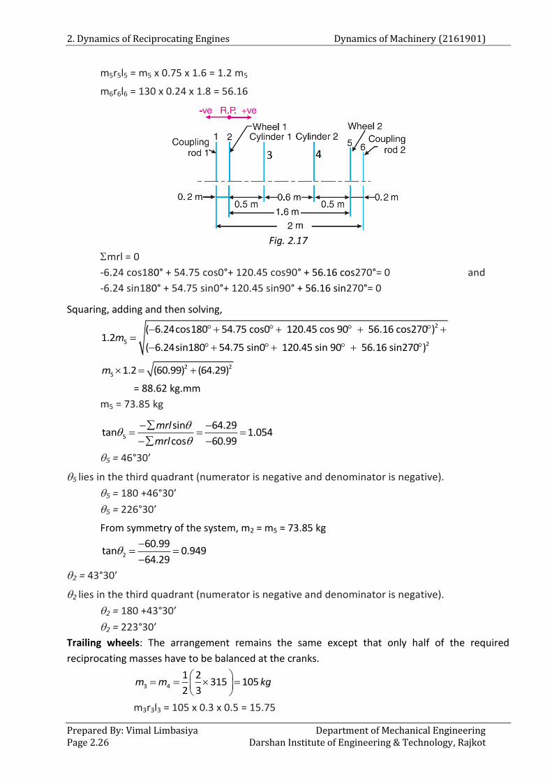
2. Dynamics of Reciprocating Engines Dynamics of Machinery (2161901)
Prepared By: Vimal Limbasiya Department of Mechanical Engineering Page 2.26 Darshan Institute of Engineering & Technology, Rajkot
m5r5l5 = m5 x 0.75 x 1.6 = 1.2 m5
m6r6l6 = 130 x 0.24 x 1.8 = 56.16
Fig. 2.17
mrl = 0
-6.24 cos180° + 54.75 cos0°+ 120.45 cos90° + 56.16 cos270°= 0 and
-6.24 sin180° + 54.75 sin0°+ 120.45 sin90° + 56.16 sin270°= 0
Squaring, adding and then solving,
2
5 2
( 6.24cos180 54.75 cos0 120.45 cos 90 56.16 cos270 )1.2
( 6.24sin180 54.75 sin0 120.45 sin 90 56.16 sin270 )m
2 25 1.2 (60.99) (64.29)m
= 88.62 kg.mm
m5 = 73.85 kg
5
sin 64.29tan 1.054
cos 60.99
mrl
mrl
5 = 46°30’
5 lies in the third quadrant (numerator is negative and denominator is negative).
5 = 180 +46°30’
5 = 226°30’
From symmetry of the system, m2 = m5 = 73.85 kg
2
60.99tan 0.949
64.29
2 = 43°30’
2 lies in the third quadrant (numerator is negative and denominator is negative).
2 = 180 +43°30’
2 = 223°30’
Trailing wheels: The arrangement remains the same except that only half of the required
reciprocating masses have to be balanced at the cranks.
3 4
1 2315 105
2 3m m kg
m3r3l3 = 105 x 0.3 x 0.5 = 15.75
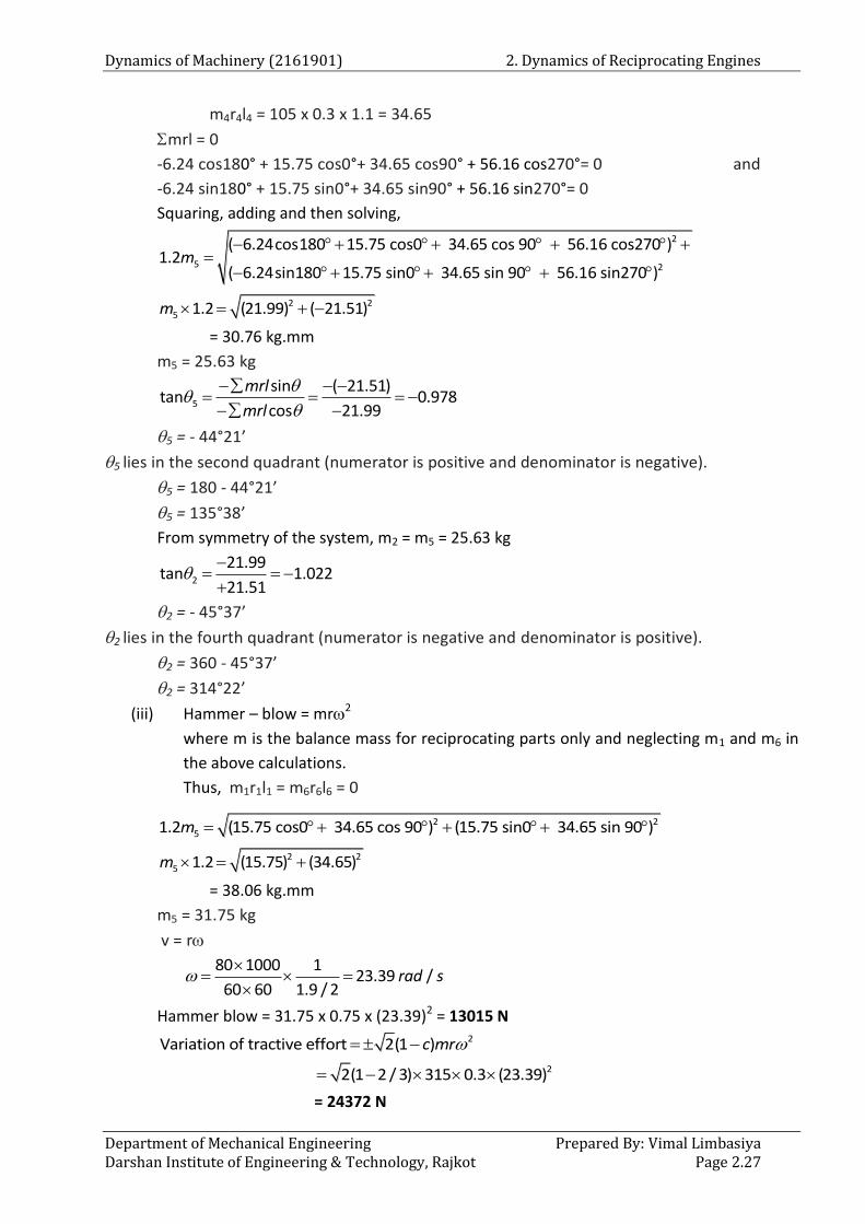
Dynamics of Machinery (2161901) 2. Dynamics of Reciprocating Engines
Department of Mechanical Engineering Prepared By: Vimal Limbasiya Darshan Institute of Engineering & Technology, Rajkot Page 2.27
m4r4l4 = 105 x 0.3 x 1.1 = 34.65
mrl = 0
-6.24 cos180° + 15.75 cos0°+ 34.65 cos90° + 56.16 cos270°= 0 and
-6.24 sin180° + 15.75 sin0°+ 34.65 sin90° + 56.16 sin270°= 0
Squaring, adding and then solving,
2
5 2
( 6.24cos180 15.75 cos0 34.65 cos 90 56.16 cos270 )1.2
( 6.24sin180 15.75 sin0 34.65 sin 90 56.16 sin270 )m
2 25 1.2 (21.99) ( 21.51)m
= 30.76 kg.mm
m5 = 25.63 kg
5
sin ( 21.51)tan 0.978
cos 21.99
mrl
mrl
5 = - 44°21’
5 lies in the second quadrant (numerator is positive and denominator is negative).
5 = 180 - 44°21’
5 = 135°38’
From symmetry of the system, m2 = m5 = 25.63 kg
2
21.99tan 1.022
21.51
2 = - 45°37’
2 lies in the fourth quadrant (numerator is negative and denominator is positive).
2 = 360 - 45°37’
2 = 314°22’
(iii) Hammer – blow = mr2
where m is the balance mass for reciprocating parts only and neglecting m1 and m6 in
the above calculations.
Thus, m1r1l1 = m6r6l6 = 0
2 251.2 (15.75 cos0 34.65 cos 90 ) (15.75 sin0 34.65 sin 90 )m
2 25 1.2 (15.75) (34.65)m
= 38.06 kg.mm
m5 = 31.75 kg
v = r
80 1000 123.39 /
60 60 1.9 / 2rad s
Hammer blow = 31.75 x 0.75 x (23.39)2 = 13015 N 2Variation of tractive effort 2(1 )c mr
22(1 2 / 3) 315 0.3 (23.39) = 24372 N
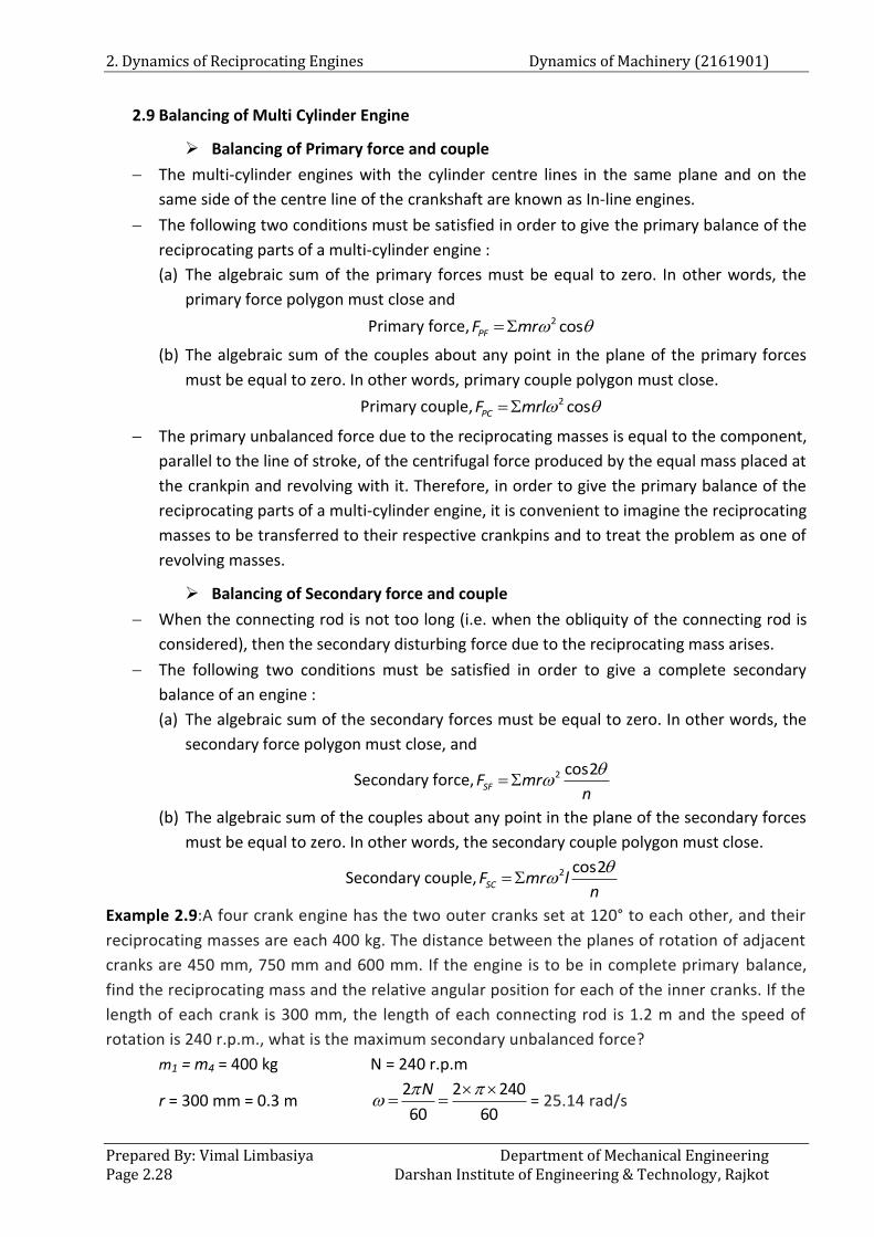
2. Dynamics of Reciprocating Engines Dynamics of Machinery (2161901)
Prepared By: Vimal Limbasiya Department of Mechanical Engineering Page 2.28 Darshan Institute of Engineering & Technology, Rajkot
2.9 Balancing of Multi Cylinder Engine
Balancing of Primary force and couple
The multi-cylinder engines with the cylinder centre lines in the same plane and on the
same side of the centre line of the crankshaft are known as In-line engines.
The following two conditions must be satisfied in order to give the primary balance of the
reciprocating parts of a multi-cylinder engine :
(a) The algebraic sum of the primary forces must be equal to zero. In other words, the
primary force polygon must close and
Primary force, 2 cosPFF mr
(b) The algebraic sum of the couples about any point in the plane of the primary forces
must be equal to zero. In other words, primary couple polygon must close.
Primary couple, 2 cosPCF mrl
The primary unbalanced force due to the reciprocating masses is equal to the component,
parallel to the line of stroke, of the centrifugal force produced by the equal mass placed at
the crankpin and revolving with it. Therefore, in order to give the primary balance of the
reciprocating parts of a multi-cylinder engine, it is convenient to imagine the reciprocating
masses to be transferred to their respective crankpins and to treat the problem as one of
revolving masses.
Balancing of Secondary force and couple
When the connecting rod is not too long (i.e. when the obliquity of the connecting rod is
considered), then the secondary disturbing force due to the reciprocating mass arises.
The following two conditions must be satisfied in order to give a complete secondary
balance of an engine :
(a) The algebraic sum of the secondary forces must be equal to zero. In other words, the
secondary force polygon must close, and
Secondary force, 2 cos2SFF mr
n
(b) The algebraic sum of the couples about any point in the plane of the secondary forces
must be equal to zero. In other words, the secondary couple polygon must close.
Secondary couple, 2 cos2SCF mr l
n
Example 2.9:A four crank engine has the two outer cranks set at 120° to each other, and their
reciprocating masses are each 400 kg. The distance between the planes of rotation of adjacent
cranks are 450 mm, 750 mm and 600 mm. If the engine is to be in complete primary balance,
find the reciprocating mass and the relative angular position for each of the inner cranks. If the
length of each crank is 300 mm, the length of each connecting rod is 1.2 m and the speed of
rotation is 240 r.p.m., what is the maximum secondary unbalanced force?
m1 = m4 = 400 kg N = 240 r.p.m
r = 300 mm = 0.3 m 2 2 240
60 60
N
= 25.14 rad/s
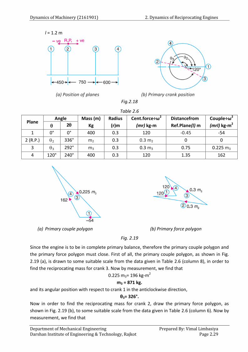
Dynamics of Machinery (2161901) 2. Dynamics of Reciprocating Engines
Department of Mechanical Engineering Prepared By: Vimal Limbasiya Darshan Institute of Engineering & Technology, Rajkot Page 2.29
l = 1.2 m
(a) Position of planes (b) Primary crank position
Fig.2.18
Table 2.6
Plane Angle Mass (m)
Kg
Radius
(r)m
Cent.force÷ω2
(mr) kg-m
Distancefrom
Ref.Plane(l) m
Couple÷ω2
(mrl) kg-m2 2
1 0° 0° 400 0.3 120 -0.45 -54
2 (R.P.) 2 336° m2 0.3 0.3 m2 0 0
3 3 292° m3 0.3 0.3 m3 0.75 0.225 m3
4 120° 240° 400 0.3 120 1.35 162
(a) Primary couple polygon (b) Primary force polygon
Fig. 2.19
Since the engine is to be in complete primary balance, therefore the primary couple polygon and
the primary force polygon must close. First of all, the primary couple polygon, as shown in Fig.
2.19 (a), is drawn to some suitable scale from the data given in Table 2.6 (column 8), in order to
find the reciprocating mass for crank 3. Now by measurement, we find that
0.225 m3= 196 kg-m2
m3 = 871 kg.
and its angular position with respect to crank 1 in the anticlockwise direction,
θ3= 326°.
Now in order to find the reciprocating mass for crank 2, draw the primary force polygon, as
shown in Fig. 2.19 (b), to some suitable scale from the data given in Table 2.6 (column 6). Now by
measurement, we find that
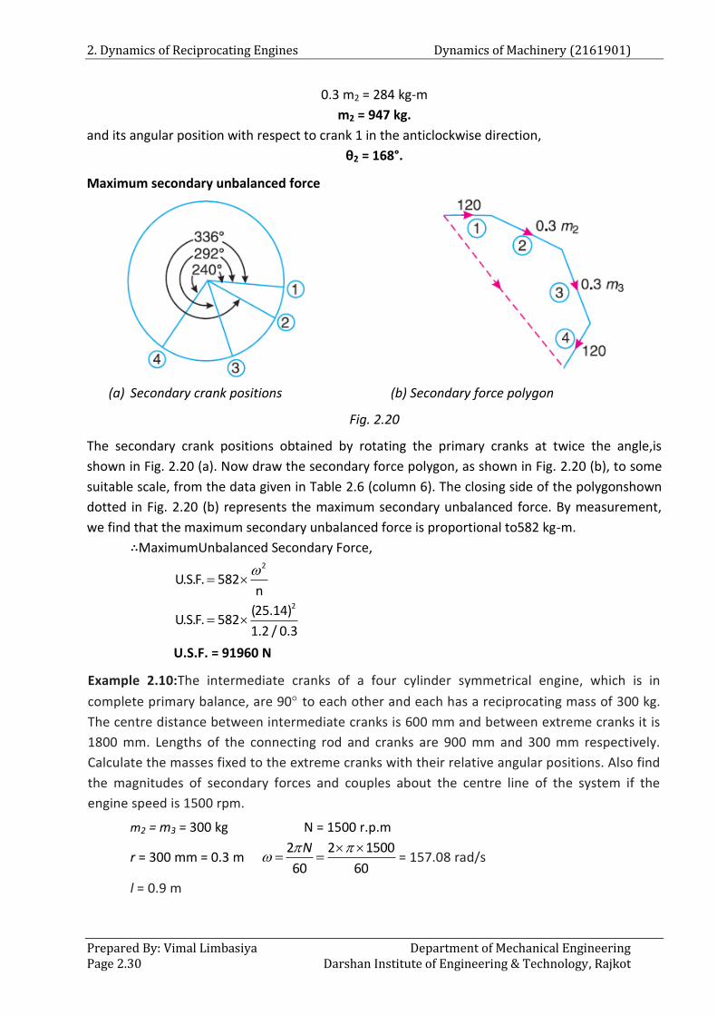
2. Dynamics of Reciprocating Engines Dynamics of Machinery (2161901)
Prepared By: Vimal Limbasiya Department of Mechanical Engineering Page 2.30 Darshan Institute of Engineering & Technology, Rajkot
0.3 m2 = 284 kg-m
m2 = 947 kg.
and its angular position with respect to crank 1 in the anticlockwise direction,
θ2 = 168°.
Maximum secondary unbalanced force
(a) Secondary crank positions (b) Secondary force polygon
Fig. 2.20
The secondary crank positions obtained by rotating the primary cranks at twice the angle,is
shown in Fig. 2.20 (a). Now draw the secondary force polygon, as shown in Fig. 2.20 (b), to some
suitable scale, from the data given in Table 2.6 (column 6). The closing side of the polygonshown
dotted in Fig. 2.20 (b) represents the maximum secondary unbalanced force. By measurement,
we find that the maximum secondary unbalanced force is proportional to582 kg-m.
∴MaximumUnbalanced Secondary Force,
2
2
U.S.F. 582n
(25.14)U.S.F. 582
1.2 / 0.3
U.S.F. = 91960 N
Example 2.10:The intermediate cranks of a four cylinder symmetrical engine, which is in
complete primary balance, are 90 to each other and each has a reciprocating mass of 300 kg.
The centre distance between intermediate cranks is 600 mm and between extreme cranks it is
1800 mm. Lengths of the connecting rod and cranks are 900 mm and 300 mm respectively.
Calculate the masses fixed to the extreme cranks with their relative angular positions. Also find
the magnitudes of secondary forces and couples about the centre line of the system if the
engine speed is 1500 rpm.
m2 = m3 = 300 kg N = 1500 r.p.m
r = 300 mm = 0.3 m 2 2 1500
60 60
N
= 157.08 rad/s
l = 0.9 m
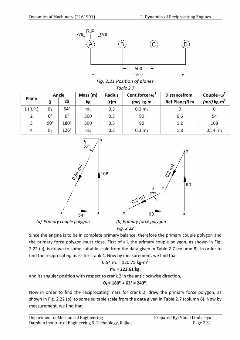
Dynamics of Machinery (2161901) 2. Dynamics of Reciprocating Engines
Department of Mechanical Engineering Prepared By: Vimal Limbasiya Darshan Institute of Engineering & Technology, Rajkot Page 2.31
Fig. 2.21 Position of planes
Table 2.7
Plane Angle Mass (m)
kg
Radius
(r)m
Cent.force÷ω2
(mr) kg-m
Distancefrom
Ref.Plane(l) m
Couple÷ω2
(mrl) kg-m2 2
1 (R.P.) 1 54° m1 0.3 0.3 m1 0 0
2 0° 0° 300 0.3 90 0.6 54
3 90° 180° 300 0.3 90 1.2 108
4 4 126° m4 0.3 0.3 m4 1.8 0.54 m4
(a) Primary couple polygon (b) Primary force polygon
Fig. 2.22
Since the engine is to be in complete primary balance, therefore the primary couple polygon and
the primary force polygon must close. First of all, the primary couple polygon, as shown in Fig.
2.22 (a), is drawn to some suitable scale from the data given in Table 2.7 (column 8), in order to
find the reciprocating mass for crank 4. Now by measurement, we find that
0.54 m4 = 120.75 kg-m2
m4 = 223.61 kg.
and its angular position with respect to crank 2 in the anticlockwise direction,
θ4 = 180 + 63° = 243.
Now in order to find the reciprocating mass for crank 2, draw the primary force polygon, as
shown in Fig. 2.22 (b), to some suitable scale from the data given in Table 2.7 (column 6). Now by
measurement, we find that
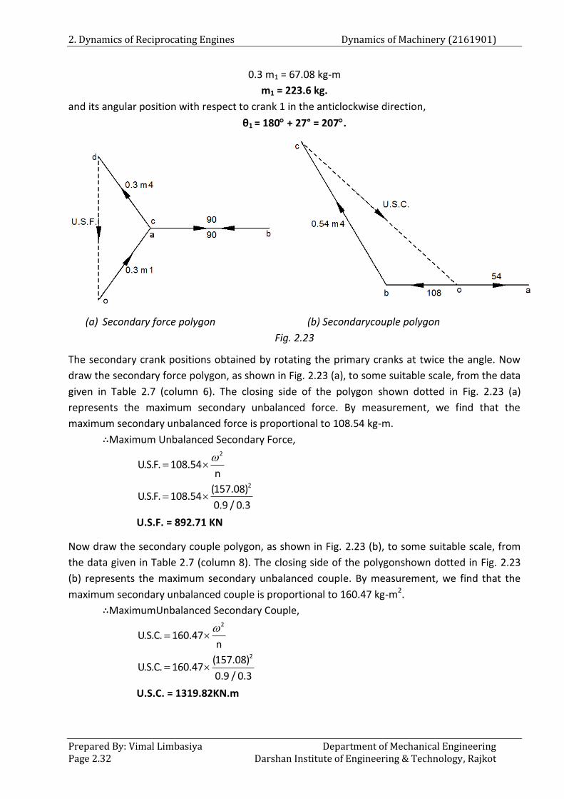
2. Dynamics of Reciprocating Engines Dynamics of Machinery (2161901)
Prepared By: Vimal Limbasiya Department of Mechanical Engineering Page 2.32 Darshan Institute of Engineering & Technology, Rajkot
0.3 m1 = 67.08 kg-m
m1 = 223.6 kg.
and its angular position with respect to crank 1 in the anticlockwise direction,
θ1 = 180 + 27° = 207.
(a) Secondary force polygon (b) Secondarycouple polygon
Fig. 2.23
The secondary crank positions obtained by rotating the primary cranks at twice the angle. Now
draw the secondary force polygon, as shown in Fig. 2.23 (a), to some suitable scale, from the data
given in Table 2.7 (column 6). The closing side of the polygon shown dotted in Fig. 2.23 (a)
represents the maximum secondary unbalanced force. By measurement, we find that the
maximum secondary unbalanced force is proportional to 108.54 kg-m.
∴Maximum Unbalanced Secondary Force, 2
2
U.S.F. 108.54n
(157.08)U.S.F. 108.54
0.9 / 0.3
U.S.F. = 892.71 KN
Now draw the secondary couple polygon, as shown in Fig. 2.23 (b), to some suitable scale, from
the data given in Table 2.7 (column 8). The closing side of the polygonshown dotted in Fig. 2.23
(b) represents the maximum secondary unbalanced couple. By measurement, we find that the
maximum secondary unbalanced couple is proportional to 160.47 kg-m2.
∴MaximumUnbalanced Secondary Couple,
2
2
U.S.C. 160.47n
(157.08)U.S.C. 160.47
0.9 / 0.3
U.S.C. = 1319.82KN.m
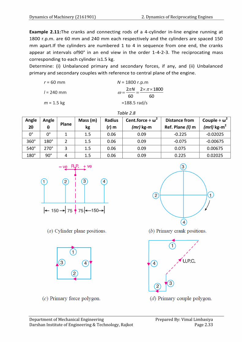
Dynamics of Machinery (2161901) 2. Dynamics of Reciprocating Engines
Department of Mechanical Engineering Prepared By: Vimal Limbasiya Darshan Institute of Engineering & Technology, Rajkot Page 2.33
Example 2.11:The cranks and connecting rods of a 4-cylinder in-line engine running at
1800 r.p.m. are 60 mm and 240 mm each respectively and the cylinders are spaced 150
mm apart.If the cylinders are numbered 1 to 4 in sequence from one end, the cranks
appear at intervals of90° in an end view in the order 1-4-2-3. The reciprocating mass
corresponding to each cylinder is1.5 kg.
Determine: (i) Unbalanced primary and secondary forces, if any, and (ii) Unbalanced
primary and secondary couples with reference to central plane of the engine.
r = 60 mm N = 1800 r.p.m
l = 240 mm 2 2 1800
60 60
N
m = 1.5 kg =188.5 rad/s
Table 2.8
Angle
2
Angle
Plane
Mass (m)
kg
Radius
(r) m
Cent.force ÷ ω2
(mr) kg-m
Distance from
Ref. Plane (l) m
Couple ÷ ω2
(mrl) kg-m2
0° 0° 1 1.5 0.06 0.09 -0.225 -0.02025
360° 180° 2 1.5 0.06 0.09 -0.075 -0.00675
540° 270° 3 1.5 0.06 0.09 0.075 0.00675
180° 90° 4 1.5 0.06 0.09 0.225 0.02025
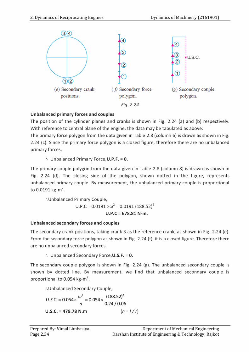
2. Dynamics of Reciprocating Engines Dynamics of Machinery (2161901)
Prepared By: Vimal Limbasiya Department of Mechanical Engineering Page 2.34 Darshan Institute of Engineering & Technology, Rajkot
Fig. 2.24
Unbalanced primary forces and couples
The position of the cylinder planes and cranks is shown in Fig. 2.24 (a) and (b) respectively.
With reference to central plane of the engine, the data may be tabulated as above:
The primary force polygon from the data given in Table 2.8 (column 6) is drawn as shown in Fig.
2.24 (c). Since the primary force polygon is a closed figure, therefore there are no unbalanced
primary forces,
∴ Unbalanced Primary Force,U.P.F. = 0.
The primary couple polygon from the data given in Table 2.8 (column 8) is drawn as shown in
Fig. 2.24 (d). The closing side of the polygon, shown dotted in the figure, represents
unbalanced primary couple. By measurement, the unbalanced primary couple is proportional
to 0.0191 kg-m2.
∴Unbalanced Primary Couple,
U.P.C = 0.0191 ×ω2 = 0.0191 (188.52)2
U.P.C = 678.81 N-m.
Unbalanced secondary forces and couples
The secondary crank positions, taking crank 3 as the reference crank, as shown in Fig. 2.24 (e).
From the secondary force polygon as shown in Fig. 2.24 (f), it is a closed figure. Therefore there
are no unbalanced secondary forces.
∴ Unbalanced Secondary Force,U.S.F. = 0.
The secondary couple polygon is shown in Fig. 2.24 (g). The unbalanced secondary couple is
shown by dotted line. By measurement, we find that unbalanced secondary couple is
proportional to 0.054 kg-m2.
∴Unbalanced Secondary Couple, 2 2(188.52)
. . . 0.054 0.0540.24 / 0.06
U S Cn
U.S.C. = 479.78 N.m (n = l / r)
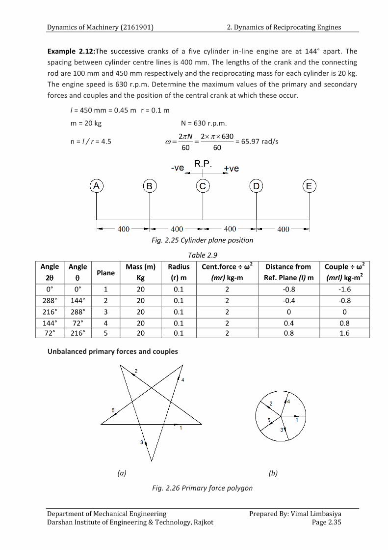
Dynamics of Machinery (2161901) 2. Dynamics of Reciprocating Engines
Department of Mechanical Engineering Prepared By: Vimal Limbasiya Darshan Institute of Engineering & Technology, Rajkot Page 2.35
Example 2.12:The successive cranks of a five cylinder in-line engine are at 144° apart. The
spacing between cylinder centre lines is 400 mm. The lengths of the crank and the connecting
rod are 100 mm and 450 mm respectively and the reciprocating mass for each cylinder is 20 kg.
The engine speed is 630 r.p.m. Determine the maximum values of the primary and secondary
forces and couples and the position of the central crank at which these occur.
l = 450 mm = 0.45 m r = 0.1 m
m = 20 kg N = 630 r.p.m.
n = l / r = 4.5 2 2 630
60 60
N
= 65.97 rad/s
Fig. 2.25 Cylinder plane position
Table 2.9
Angle
2
Angle
Plane
Mass (m)
Kg
Radius
(r) m
Cent.force ÷ ω2
(mr) kg-m
Distance from
Ref. Plane (l) m
Couple ÷ ω2
(mrl) kg-m2
0° 0° 1 20 0.1 2 -0.8 -1.6
288° 144° 2 20 0.1 2 -0.4 -0.8
216° 288° 3 20 0.1 2 0 0
144° 72° 4 20 0.1 2 0.4 0.8
72° 216° 5 20 0.1 2 0.8 1.6
Unbalanced primary forces and couples
(a) (b)
Fig. 2.26 Primary force polygon
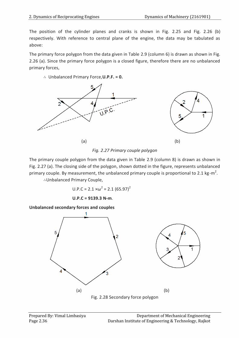
2. Dynamics of Reciprocating Engines Dynamics of Machinery (2161901)
Prepared By: Vimal Limbasiya Department of Mechanical Engineering Page 2.36 Darshan Institute of Engineering & Technology, Rajkot
The position of the cylinder planes and cranks is shown in Fig. 2.25 and Fig. 2.26 (b)
respectively. With reference to central plane of the engine, the data may be tabulated as
above:
The primary force polygon from the data given in Table 2.9 (column 6) is drawn as shown in Fig.
2.26 (a). Since the primary force polygon is a closed figure, therefore there are no unbalanced
primary forces,
∴ Unbalanced Primary Force,U.P.F. = 0.
(a) (b)
Fig. 2.27 Primary couple polygon
The primary couple polygon from the data given in Table 2.9 (column 8) is drawn as shown in
Fig. 2.27 (a). The closing side of the polygon, shown dotted in the figure, represents unbalanced
primary couple. By measurement, the unbalanced primary couple is proportional to 2.1 kg-m2.
∴Unbalanced Primary Couple,
U.P.C = 2.1 ×ω2 = 2.1 (65.97)2
U.P.C = 9139.3 N-m.
Unbalanced secondary forces and couples
(a) (b)
Fig. 2.28 Secondary force polygon
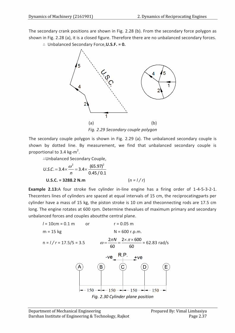
Dynamics of Machinery (2161901) 2. Dynamics of Reciprocating Engines
Department of Mechanical Engineering Prepared By: Vimal Limbasiya Darshan Institute of Engineering & Technology, Rajkot Page 2.37
The secondary crank positions are shown in Fig. 2.28 (b). From the secondary force polygon as
shown in Fig. 2.28 (a), it is a closed figure. Therefore there are no unbalanced secondary forces.
∴ Unbalanced Secondary Force,U.S.F. = 0.
(a) (b)
Fig. 2.29 Secondary couple polygon
The secondary couple polygon is shown in Fig. 2.29 (a). The unbalanced secondary couple is
shown by dotted line. By measurement, we find that unbalanced secondary couple is
proportional to 3.4 kg-m2.
∴Unbalanced Secondary Couple, 2 2(65.97)
. . . 3.4 3.40.45 / 0.1
U S Cn
U.S.C. = 3288.2 N.m (n = l / r)
Example 2.13:A four stroke five cylinder in-line engine has a firing order of 1-4-5-3-2-1.
Thecenters lines of cylinders are spaced at equal intervals of 15 cm, the reciprocatingparts per
cylinder have a mass of 15 kg, the piston stroke is 10 cm and theconnecting rods are 17.5 cm
long. The engine rotates at 600 rpm. Determine thevalues of maximum primary and secondary
unbalanced forces and couples aboutthe central plane.
l = 10cm = 0.1 m or r = 0.05 m
m = 15 kg N = 600 r.p.m.
n = l / r = 17.5/5 = 3.5 2 2 600
60 60
N
= 62.83 rad/s
Fig. 2.30 Cylinder plane position
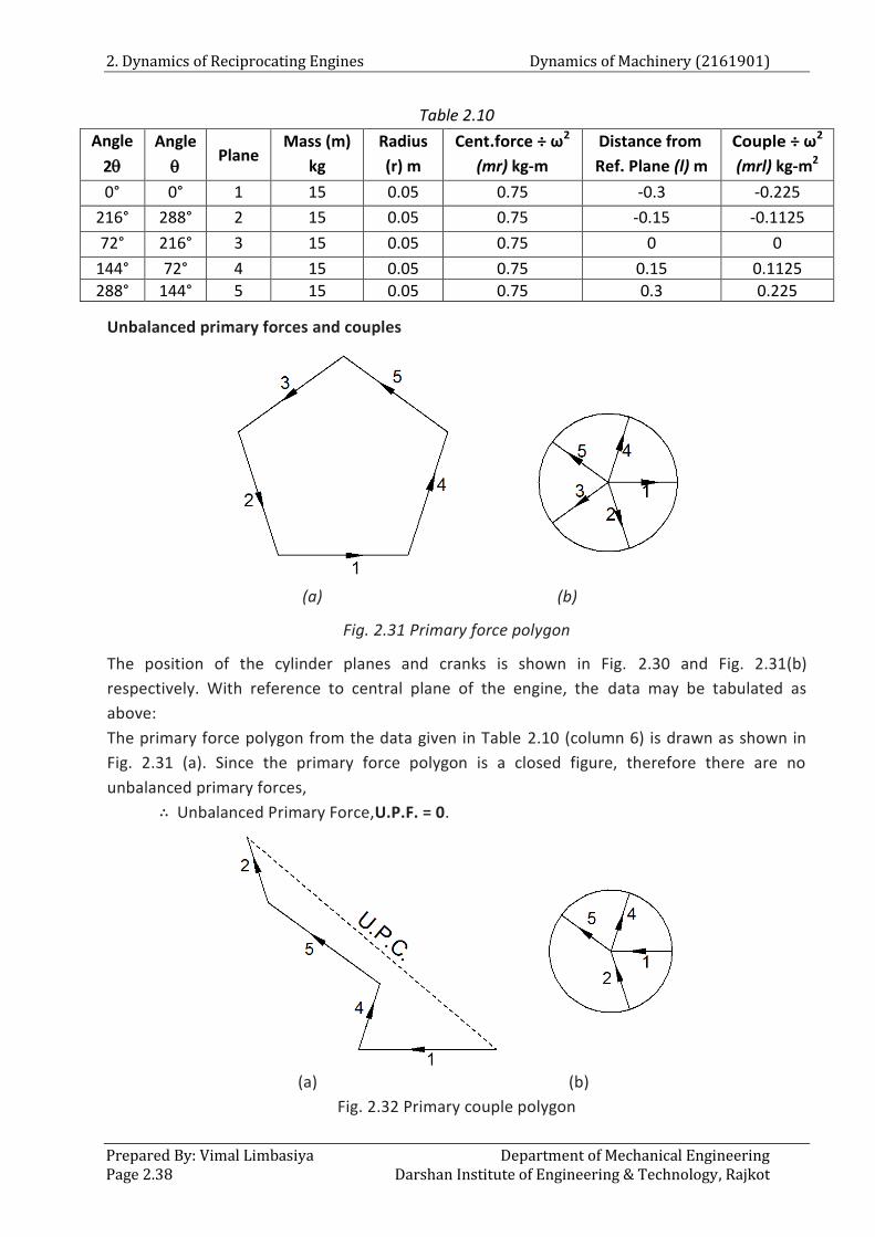
2. Dynamics of Reciprocating Engines Dynamics of Machinery (2161901)
Prepared By: Vimal Limbasiya Department of Mechanical Engineering Page 2.38 Darshan Institute of Engineering & Technology, Rajkot
Table 2.10
Angle
2
Angle
Plane
Mass (m)
kg
Radius
(r) m
Cent.force ÷ ω2
(mr) kg-m
Distance from
Ref. Plane (l) m
Couple ÷ ω2
(mrl) kg-m2
0° 0° 1 15 0.05 0.75 -0.3 -0.225
216° 288° 2 15 0.05 0.75 -0.15 -0.1125
72° 216° 3 15 0.05 0.75 0 0
144° 72° 4 15 0.05 0.75 0.15 0.1125
288° 144° 5 15 0.05 0.75 0.3 0.225
Unbalanced primary forces and couples
(a) (b)
Fig. 2.31 Primary force polygon
The position of the cylinder planes and cranks is shown in Fig. 2.30 and Fig. 2.31(b)
respectively. With reference to central plane of the engine, the data may be tabulated as
above:
The primary force polygon from the data given in Table 2.10 (column 6) is drawn as shown in
Fig. 2.31 (a). Since the primary force polygon is a closed figure, therefore there are no
unbalanced primary forces,
∴ Unbalanced Primary Force,U.P.F. = 0.
(a) (b)
Fig. 2.32 Primary couple polygon
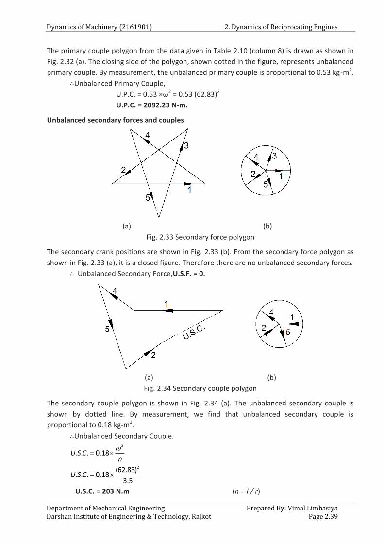
Dynamics of Machinery (2161901) 2. Dynamics of Reciprocating Engines
Department of Mechanical Engineering Prepared By: Vimal Limbasiya Darshan Institute of Engineering & Technology, Rajkot Page 2.39
The primary couple polygon from the data given in Table 2.10 (column 8) is drawn as shown in
Fig. 2.32 (a). The closing side of the polygon, shown dotted in the figure, represents unbalanced
primary couple. By measurement, the unbalanced primary couple is proportional to 0.53 kg-m2.
∴Unbalanced Primary Couple,
U.P.C. = 0.53 ×ω2 = 0.53 (62.83)2
U.P.C. = 2092.23 N-m.
Unbalanced secondary forces and couples
(a) (b)
Fig. 2.33 Secondary force polygon
The secondary crank positions are shown in Fig. 2.33 (b). From the secondary force polygon as
shown in Fig. 2.33 (a), it is a closed figure. Therefore there are no unbalanced secondary forces.
∴ Unbalanced Secondary Force,U.S.F. = 0.
(a) (b)
Fig. 2.34 Secondary couple polygon
The secondary couple polygon is shown in Fig. 2.34 (a). The unbalanced secondary couple is
shown by dotted line. By measurement, we find that unbalanced secondary couple is
proportional to 0.18 kg-m2.
∴Unbalanced Secondary Couple, 2
2
. . . 0.18
(62.83). . . 0.18
3.5
U S Cn
U S C
U.S.C. = 203 N.m (n = l / r)
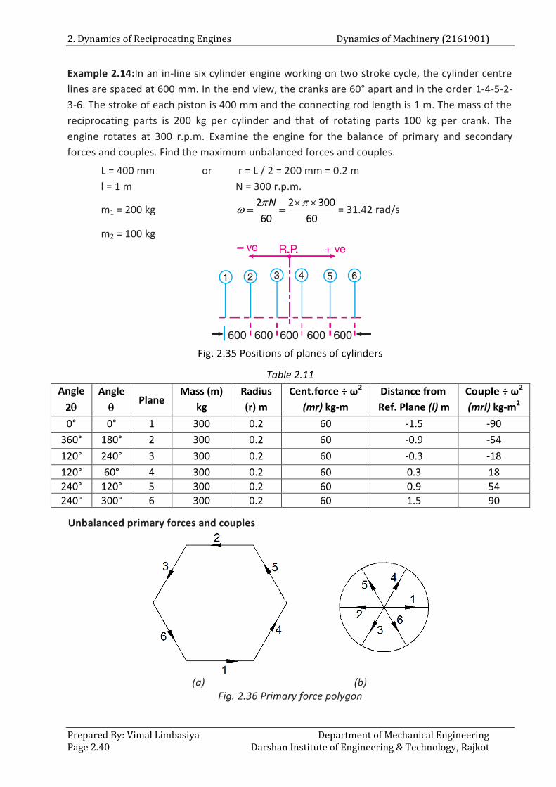
2. Dynamics of Reciprocating Engines Dynamics of Machinery (2161901)
Prepared By: Vimal Limbasiya Department of Mechanical Engineering Page 2.40 Darshan Institute of Engineering & Technology, Rajkot
Example 2.14:In an in-line six cylinder engine working on two stroke cycle, the cylinder centre
lines are spaced at 600 mm. In the end view, the cranks are 60° apart and in the order 1-4-5-2-
3-6. The stroke of each piston is 400 mm and the connecting rod length is 1 m. The mass of the
reciprocating parts is 200 kg per cylinder and that of rotating parts 100 kg per crank. The
engine rotates at 300 r.p.m. Examine the engine for the balance of primary and secondary
forces and couples. Find the maximum unbalanced forces and couples.
L = 400 mm or r = L / 2 = 200 mm = 0.2 m
l = 1 m N = 300 r.p.m.
m1 = 200 kg 2 2 300
60 60
N
= 31.42 rad/s
m2 = 100 kg
Fig. 2.35 Positions of planes of cylinders
Table 2.11
Angle
2
Angle
Plane
Mass (m)
kg
Radius
(r) m
Cent.force ÷ ω2
(mr) kg-m
Distance from
Ref. Plane (l) m
Couple ÷ ω2
(mrl) kg-m2
0° 0° 1 300 0.2 60 -1.5 -90
360° 180° 2 300 0.2 60 -0.9 -54
120° 240° 3 300 0.2 60 -0.3 -18
120° 60° 4 300 0.2 60 0.3 18
240° 120° 5 300 0.2 60 0.9 54
240° 300° 6 300 0.2 60 1.5 90
Unbalanced primary forces and couples
(a) (b)
Fig. 2.36 Primary force polygon
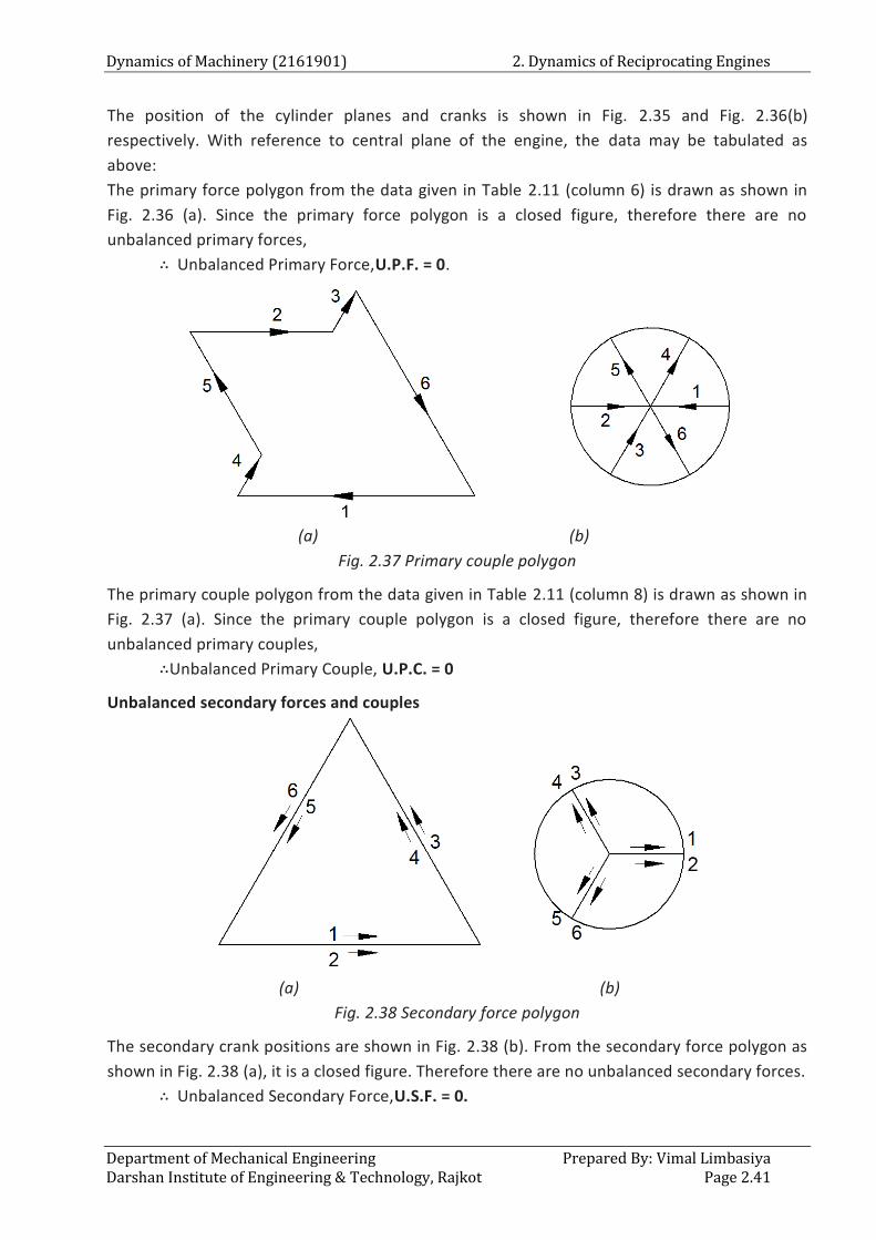
Dynamics of Machinery (2161901) 2. Dynamics of Reciprocating Engines
Department of Mechanical Engineering Prepared By: Vimal Limbasiya Darshan Institute of Engineering & Technology, Rajkot Page 2.41
The position of the cylinder planes and cranks is shown in Fig. 2.35 and Fig. 2.36(b)
respectively. With reference to central plane of the engine, the data may be tabulated as
above:
The primary force polygon from the data given in Table 2.11 (column 6) is drawn as shown in
Fig. 2.36 (a). Since the primary force polygon is a closed figure, therefore there are no
unbalanced primary forces,
∴ Unbalanced Primary Force,U.P.F. = 0.
(a) (b)
Fig. 2.37 Primary couple polygon
The primary couple polygon from the data given in Table 2.11 (column 8) is drawn as shown in
Fig. 2.37 (a). Since the primary couple polygon is a closed figure, therefore there are no
unbalanced primary couples,
∴Unbalanced Primary Couple, U.P.C. = 0
Unbalanced secondary forces and couples
(a) (b)
Fig. 2.38 Secondary force polygon
The secondary crank positions are shown in Fig. 2.38 (b). From the secondary force polygon as
shown in Fig. 2.38 (a), it is a closed figure. Therefore there are no unbalanced secondary forces.
∴ Unbalanced Secondary Force,U.S.F. = 0.
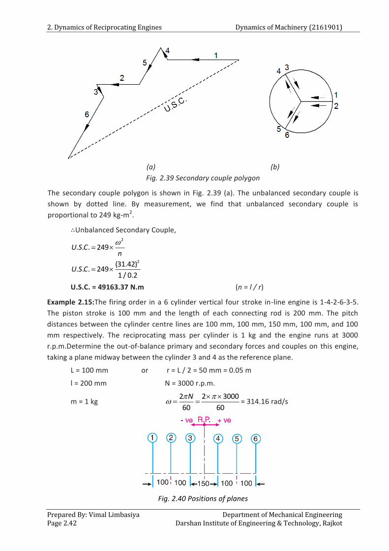
2. Dynamics of Reciprocating Engines Dynamics of Machinery (2161901)
Prepared By: Vimal Limbasiya Department of Mechanical Engineering Page 2.42 Darshan Institute of Engineering & Technology, Rajkot
(a) (b)
Fig. 2.39 Secondary couple polygon
The secondary couple polygon is shown in Fig. 2.39 (a). The unbalanced secondary couple is
shown by dotted line. By measurement, we find that unbalanced secondary couple is
proportional to 249 kg-m2.
∴Unbalanced Secondary Couple, 2
2
. . . 249
(31.42). . . 249
1 / 0.2
U S Cn
U S C
U.S.C. = 49163.37 N.m (n = l / r)
Example 2.15:The firing order in a 6 cylinder vertical four stroke in-line engine is 1-4-2-6-3-5.
The piston stroke is 100 mm and the length of each connecting rod is 200 mm. The pitch
distances between the cylinder centre lines are 100 mm, 100 mm, 150 mm, 100 mm, and 100
mm respectively. The reciprocating mass per cylinder is 1 kg and the engine runs at 3000
r.p.m.Determine the out-of-balance primary and secondary forces and couples on this engine,
taking a plane midway between the cylinder 3 and 4 as the reference plane.
L = 100 mm or r = L / 2 = 50 mm = 0.05 m
l = 200 mm N = 3000 r.p.m.
m = 1 kg 2 2 3000
60 60
N
= 314.16 rad/s
Fig. 2.40 Positions of planes
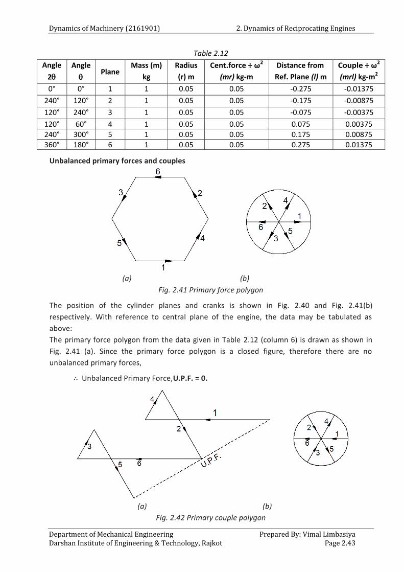
Dynamics of Machinery (2161901) 2. Dynamics of Reciprocating Engines
Department of Mechanical Engineering Prepared By: Vimal Limbasiya Darshan Institute of Engineering & Technology, Rajkot Page 2.43
Table 2.12
Angle
2
Angle
Plane
Mass (m)
kg
Radius
(r) m
Cent.force ÷ ω2
(mr) kg-m
Distance from
Ref. Plane (l) m
Couple ÷ ω2
(mrl) kg-m2
0° 0° 1 1 0.05 0.05 -0.275 -0.01375
240° 120° 2 1 0.05 0.05 -0.175 -0.00875
120° 240° 3 1 0.05 0.05 -0.075 -0.00375
120° 60° 4 1 0.05 0.05 0.075 0.00375
240° 300° 5 1 0.05 0.05 0.175 0.00875
360° 180° 6 1 0.05 0.05 0.275 0.01375
Unbalanced primary forces and couples
(a) (b)
Fig. 2.41 Primary force polygon
The position of the cylinder planes and cranks is shown in Fig. 2.40 and Fig. 2.41(b)
respectively. With reference to central plane of the engine, the data may be tabulated as
above:
The primary force polygon from the data given in Table 2.12 (column 6) is drawn as shown in
Fig. 2.41 (a). Since the primary force polygon is a closed figure, therefore there are no
unbalanced primary forces,
∴ Unbalanced Primary Force,U.P.F. = 0.
(a) (b)
Fig. 2.42 Primary couple polygon

2. Dynamics of Reciprocating Engines Dynamics of Machinery (2161901)
Prepared By: Vimal Limbasiya Department of Mechanical Engineering Page 2.44 Darshan Institute of Engineering & Technology, Rajkot
The primary couple polygon from the data given in Table 2.12 (column 8) is drawn as shown in
Fig. 2.42 (a). The closing side of the polygon, shown dotted in the figure, represents unbalanced
primary couple. By measurement, the unbalanced primary couple is proportional to 0.01732
kg-m2.
∴Unbalanced Primary Couple,
U.P.C. = 0.01732 ×ω2 = 0.01732 (314.16)2
U.P.C.= 1709.42 N-m.
Unbalanced secondary forces and couples
(a) (b)
Fig. 2.43 Secondary force polygon
The secondary crank positions are shown in Fig. 2.43 (b). From the secondary force polygon as
shown in Fig. 2.43 (a), it is a closed figure. Therefore there are no unbalanced secondary forces.
∴ Unbalanced Secondary Force,U.S.F. = 0.
(a) (b)
Fig. 2.44 Secondary couple polygon
The secondary couple polygon is drawn as shown in Fig. 2.44 (a). Since the secondarycouple
polygon is a closed figure, therefore there are no unbalanced secondary couples,
∴Unbalanced Secondary Couple, U.S.C. = 0
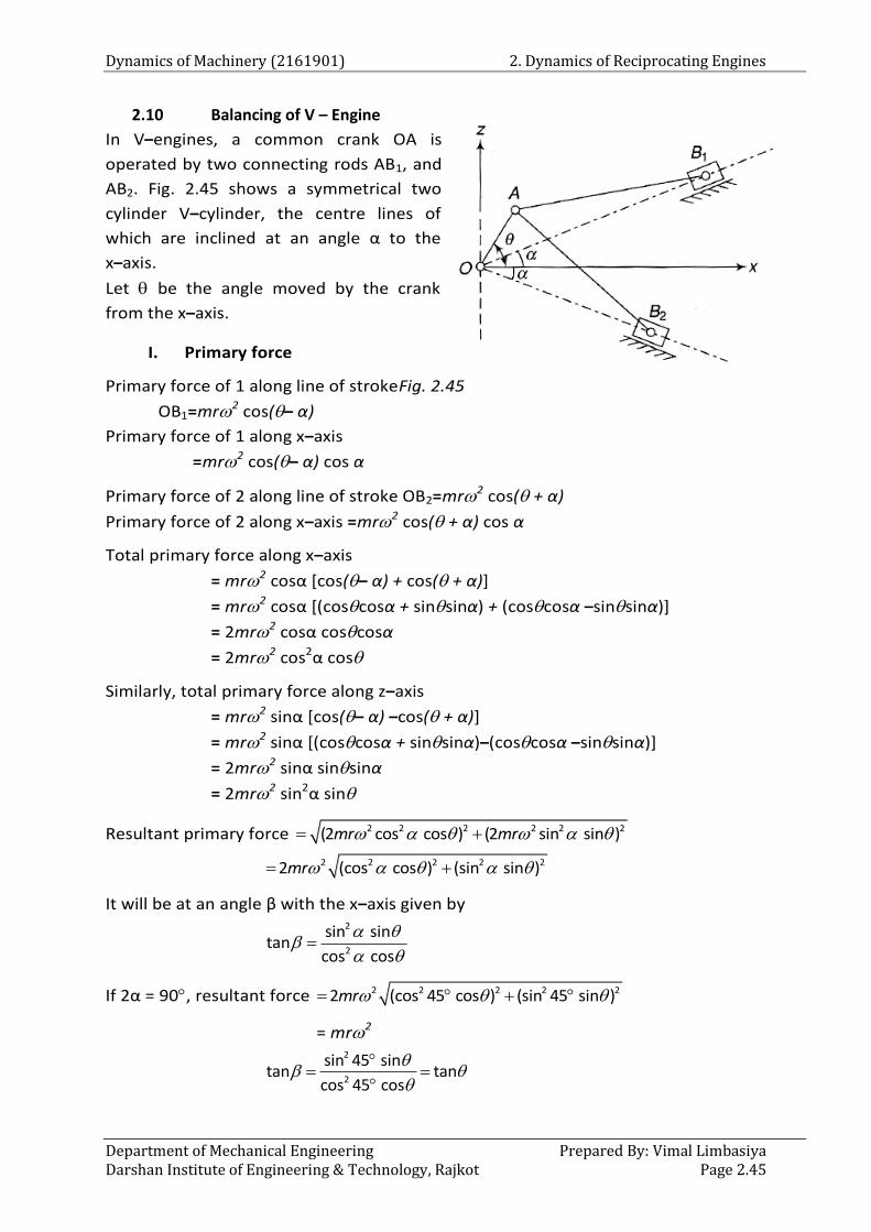
Dynamics of Machinery (2161901) 2. Dynamics of Reciprocating Engines
Department of Mechanical Engineering Prepared By: Vimal Limbasiya Darshan Institute of Engineering & Technology, Rajkot Page 2.45
2.10 Balancing of V – Engine
In V–engines, a common crank OA is
operated by two connecting rods AB1, and
AB2. Fig. 2.45 shows a symmetrical two
cylinder V–cylinder, the centre lines of
which are inclined at an angle α to the
x–axis.
Let be the angle moved by the crank
from the x–axis.
I. Primary force
Primary force of 1 along line of strokeFig. 2.45
OB1=mr2 cos(– α)
Primary force of 1 along x–axis
=mr2 cos(– α) cos α
Primary force of 2 along line of stroke OB2=mr2 cos( + α)
Primary force of 2 along x–axis =mr2 cos( + α) cos α
Total primary force along x–axis
= mr2 cosα *cos(– α) + cos( + α)]
= mr2 cosα *(coscosα + sinsinα) + (coscosα –sinsinα)]
= 2mr2 cosα coscosα
= 2mr2 cos2α cos
Similarly, total primary force along z–axis
= mr2 sinα *cos(– α) –cos( + α)]
= mr2 sinα *(coscosα + sinsinα)–(coscosα –sinsinα)]
= 2mr2 sinα sinsinα
= 2mr2 sin2α sin
Resultant primary force 2 2 2 2 2 2(2 cos ) (2cos sin sin )mr mr
2 2 2 2 22 ( cos ) ( sin )cos sinmr
It will be at an angle β with the x–axis given by 2
2
sisin
cos
ntan
cos
If 2α = 90, resultant force 2 2 2 2 22 ( cos )cos ( s45 s in )in 45mr
= mr2 2
2
sin
c
45 sintan tan
45 cosos
2. Dynamics of Reciprocating Engines Dynamics of Machinery (2161901)
Prepared By: Vimal Limbasiya Department of Mechanical Engineering Page 2.46 Darshan Institute of Engineering & Technology, Rajkot
i.e., β = or it acts along the crank and, therefore, can be completely balanced by a mass
at a suitable radius diametrically opposite to the crank such that mrrr = mr.
For a given value of α, the resultant primary force is maximum when
2 2 2 2(cos sin cos ) ( sin ) is maximum 4 2 4 2(cos sin cos sin ) is maximum
4 2 4 2( cos sin ) 0cos sind
d
4 4cos .2 scos sin 2 sin cn 0i . os
4 4cos . ssin2 sinin 2 0.
4 4sisin2 ( 0n cos )
As α is not zero, therefore, for a given value of α, the resultant primary force is maximum
when is zero degree.
II. Secondary force
Secondary force of 1 along OB1
2
cos2( )mr
n
Secondary force of 1 along x-axis 2
cos2( )cosmr
n
Secondary force of 2 along OB2
2
cos2( )mr
n
Secondary force of 2 along x-axis 2
cos2( )cosmr
n
Total secondary force along x-axis 2
cos [cos2( ) cos2( )]mr
n
2
cos [(cos2 cos2 sin2 sin2 ) (cos2 cos2 sin2 sin2 )]mr
n
22cos cos2 cos2
mr
n
Similarly, secondary force along z-axis22
sin sin2 sin2mr
n
Resultant secondary force 2
2 22(cos cos2 cos2 ) (sin sin2 sin2 )
mr
n
sin sin2
co
sin2tan '
s cos2cos2
If 2α = 90 or α = 45
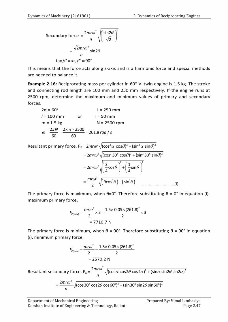
Dynamics of Machinery (2161901) 2. Dynamics of Reciprocating Engines
Department of Mechanical Engineering Prepared By: Vimal Limbasiya Darshan Institute of Engineering & Technology, Rajkot Page 2.47
Secondary force
222 sin2
2
mr
n
22
sin2mr
n
tan ' , ' 90
This means that the force acts along z-axis and is a harmonic force and special methods
are needed to balance it.
Example 2.16: Reciprocating mass per cylinder in 60 V–twin engine is 1.5 kg. The stroke
and connecting rod length are 100 mm and 250 mm respectively. If the engine runs at
2500 rpm, determine the maximum and minimum values of primary and secondary
forces.
2α = 60 L = 250 mm
l = 100 mm or r = 50 mm
m = 1.5 kg N = 2500 rpm
2 2 2500
261.8 /60 60
Nrad s
Resultant primary force, FP2 2 2 2 22 ( cos ) ( sin )cos sinmr
2 2 2 2 22 ( cos )cos ( s30 s in )in 30mr
2 2
2 3 12 cos sin
4 4mr
2
2 29cos sin2
mr ……………………….(i)
The primary force is maximum, when θ=0°. Therefore substituting θ = 0° in equation (i),
maximum primary force,
2 2
(max)
1.5 0.05 (261.8)3 3
2 2P
mrF
= 7710.7 N
The primary force is minimum, when θ = 90°. Therefore substituting θ = 90° in equation
(i), minimum primary force,
2 2
(min)
1.5 0.05 (261.8)
2 2P
mrF
= 2570.2 N
Resultant secondary force, FS
22 22
(cos cos2 cos2 ) (sin sin2 sin2 )mr
n
2
2 22(cos30 cos2 cos60 ) (sin30 sin2 sin60 )
mr
n
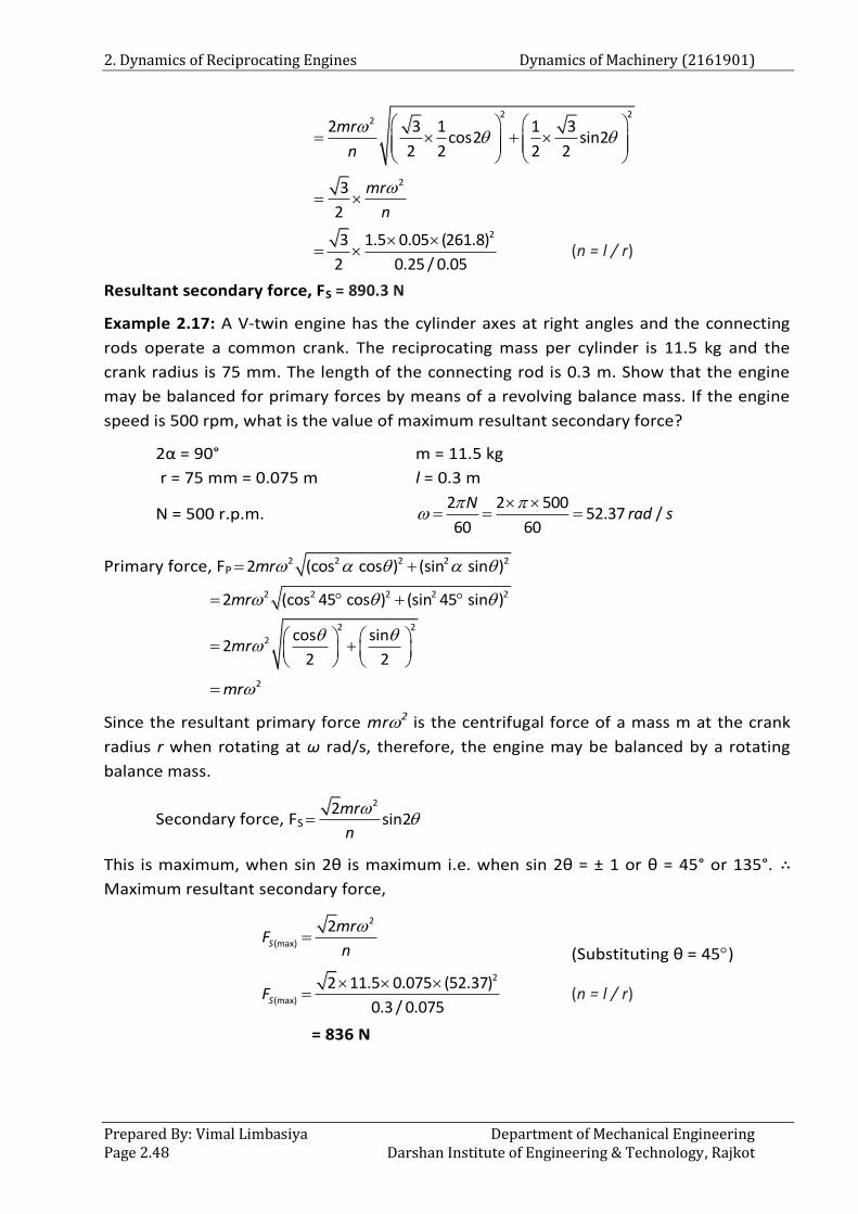
2. Dynamics of Reciprocating Engines Dynamics of Machinery (2161901)
Prepared By: Vimal Limbasiya Department of Mechanical Engineering Page 2.48 Darshan Institute of Engineering & Technology, Rajkot
2 222 3 1 1 3
cos2 sin22 2 2 2
mr
n
23
2
mr
n
23 1.5 0.05 (261.8)
2 0.25 / 0.05
(n = l / r)
Resultant secondary force, FS = 890.3 N
Example 2.17: A V-twin engine has the cylinder axes at right angles and the connecting
rods operate a common crank. The reciprocating mass per cylinder is 11.5 kg and the
crank radius is 75 mm. The length of the connecting rod is 0.3 m. Show that the engine
may be balanced for primary forces by means of a revolving balance mass. If the engine
speed is 500 rpm, what is the value of maximum resultant secondary force?
2α = 90° m = 11.5 kg
r = 75 mm = 0.075 m l = 0.3 m
N = 500 r.p.m. 2 2 500
52.37 /60 60
Nrad s
Primary force, FP2 2 2 2 22 ( cos ) ( sin )cos sinmr
2 2 2 2 22 ( cos )cos ( s45 s in )in 45mr
2 2
2 cos sin2
2 2mr
2mr
Since the resultant primary force mr2 is the centrifugal force of a mass m at the crank
radius r when rotating at ω rad/s, therefore, the engine may be balanced by a rotating
balance mass.
Secondary force, FS
22sin2
mr
n
This is maximum, when sin 2θ is maximum i.e. when sin 2θ = ± 1 or θ = 45° or 135°. ∴
Maximum resultant secondary force,
2
(max)
2S
mrF
n
(Substituting θ = 45) 2
(max)
2 11.5 0.075 (52.37)
0.3 / 0.075SF
(n = l / r)
= 836 N
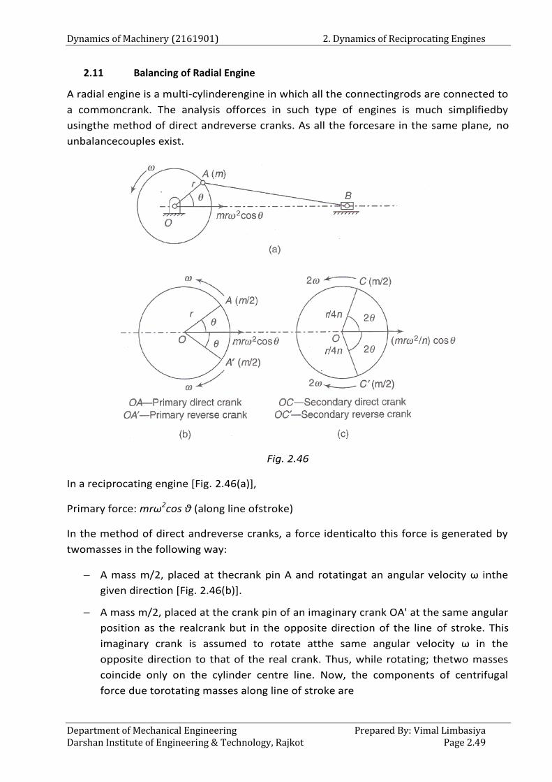
Dynamics of Machinery (2161901) 2. Dynamics of Reciprocating Engines
Department of Mechanical Engineering Prepared By: Vimal Limbasiya Darshan Institute of Engineering & Technology, Rajkot Page 2.49
2.11 Balancing of Radial Engine
A radial engine is a multi-cylinderengine in which all the connectingrods are connected to
a commoncrank. The analysis offorces in such type of engines is much simplifiedby
usingthe method of direct andreverse cranks. As all the forcesare in the same plane, no
unbalancecouples exist.
Fig. 2.46
In a reciprocating engine [Fig. 2.46(a)],
Primary force: mrω2cos θ (along line ofstroke)
In the method of direct andreverse cranks, a force identicalto this force is generated by
twomasses in the following way:
A mass m/2, placed at thecrank pin A and rotatingat an angular velocity ω inthe
given direction [Fig. 2.46(b)].
A mass m/2, placed at the crank pin of an imaginary crank OA' at the same angular
position as the realcrank but in the opposite direction of the line of stroke. This
imaginary crank is assumed to rotate atthe same angular velocity ω in the
opposite direction to that of the real crank. Thus, while rotating; thetwo masses
coincide only on the cylinder centre line. Now, the components of centrifugal
force due torotating masses along line of stroke are
2. Dynamics of Reciprocating Engines Dynamics of Machinery (2161901)
Prepared By: Vimal Limbasiya Department of Mechanical Engineering Page 2.50 Darshan Institute of Engineering & Technology, Rajkot
Due to mass at A 2 cos2
mr
Due to mass at A’ 2 cos2
mr
Thus, total force along line of stroke = mrω2cos θ which is equal to the primary force. At
any instant, the components of the centrifugal forces of these two masses normal to the
line of stroke will be equal and opposite.
The crank rotating in the direction of engine rotation is known as the direct crank andthe
imaginary crank rotating in the opposite direction is known as the reverse crank.
Secondary accelerating force 2 2cos2 cos2(2 )
4mr mr
n n
2(2 ) cos24
rm
n (along line of stroke)
This force can also be generated by two masses in a similar way as follows:
A mass m/2, placed at the end of direct secondary crank of length r/(4n) at angle
2 and rotating at an angular velocity 2 in the given direction [Fig. 6.1(c)].
A mass m/2, placed at the end of reverse secondary crank of length r/(4n) at angle
-2 rotating at an angular velocity 2 in the opposite direction. Now, the
components of centrifugal force due to rotating masses along line of stroke are
Due to mass at 2
2(2 ) cos2 cos22 4 2
m r mrC
n n
Due to mass at 2
2' (2 ) cos2 cos22 4 2
m r mrC
n n
Thus total force along line of stroke 2
22 (2 ) cos2 cos22 4
m r mr
n n
Which is equal to the secondary force.
Department of Mechanical Engineering Prepared by: Mr. SUNIL G. JANIYANI Darshan Institute of Engineering & Technology, Rajkot Page 3.1
3 Longitudinal and Transverse Vibrations
Course Contents
3.1 Introduction to Vibrations
3.2 Natural Frequency of Free
Longitudinal Vibrations
3.3 Natural Frequency of Free
Transverse Vibrations
3.4 Natural Frequency of Free
Transverse Vibrations Due to
a Point Load Acting Over a
Simply Supported Shaft
3.5 Critical or Whirling Speed of
Shaft
3.6 Frequency of Free Damped
Vibrations (Viscous Damping)
3.7 Damping Factor or Damping
Ratio
3.8 Logarithmic decrement
3.9 Magnification factor or
dynamic magnifier
3.10 Vibration isolation and
Transmissibility
Examples
3. Longitudinal and Transverse Vibrations Dynamics of Machinery (2161901)
Prepared by: Mr. SUNIL G. JANIYANI Department of Mechanical Engineering Page 3.2 Darshan Institute of Engineering & Technology, Rajkot
3.1 Introduction to Vibrations
When elastic bodies such as a spring, a beam and a shaft are displaced from the
equilibrium position by the application of external forces, and then released, they
execute a vibratory motion.
This is due to the reason that, when a body is displaced, the internal forces in the
form of elastic or strain energy are present in the body. At release, these forces bring
the body to its original position.
When the body reaches the equilibrium position, the whole of the elastic or strain
energy is converted into kinetic energy due to which the body continues to move in
the opposite direction.
The whole of the kinetic energy is again converted into strain energy due to which
the body again returns to the equilibrium position.
In this way, the vibratory motion is repeated indefinitely.
3.1.1 Terminology
The following terms are commonly used in connection with the vibratory motions:
(i) Period of vibration or time period: It is the time interval after which the
motion is repeated itself. The period of vibration is usually expressed in
seconds.
(ii) Cycle: It is the motion completed during one-time period.
(iii) Frequency: It is the number of cycles described in one second. In S.I. units,
the frequency is expressed in hertz (briefly written as Hz) which is equal to
one cycle per second.
3.1.2 Types of Vibratory Motion
(i) Free or natural vibrations: When no external force acts on the body, after
giving it an initial displacement, then the body is said to be under free or
natural vibrations.
The frequency of the free vibrations is called free or natural frequency.
(ii) Forced vibrations: When the body vibrates under the influence of external
force, then the body is said to be under forced vibrations.
The external force applied to the body is a periodic disturbing force created
by unbalance. The vibrations have the same frequency as the applied force.
Note: When the frequency of the external force is same as that of the natural
vibrations, resonance takes place.
(iii) Damped vibrations: When there is a reduction in amplitude over every cycle
of vibration, the motion is said to be damped vibration.
This is due to the fact that a certain amount of energy possessed by the
vibrating system is always dissipated in overcoming frictional resistances to
the motion.
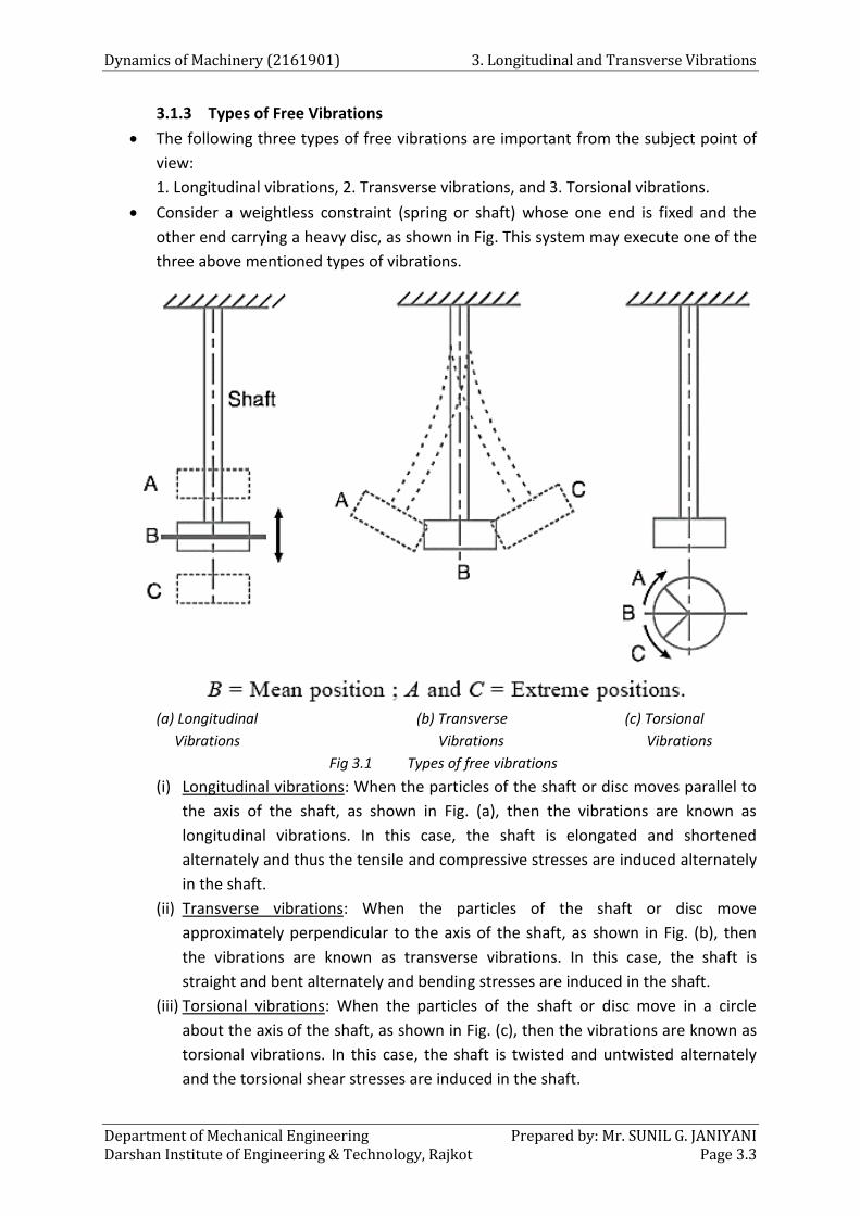
Dynamics of Machinery (2161901) 3. Longitudinal and Transverse Vibrations
Department of Mechanical Engineering Prepared by: Mr. SUNIL G. JANIYANI Darshan Institute of Engineering & Technology, Rajkot Page 3.3
3.1.3 Types of Free Vibrations
The following three types of free vibrations are important from the subject point of
view:
1. Longitudinal vibrations, 2. Transverse vibrations, and 3. Torsional vibrations.
Consider a weightless constraint (spring or shaft) whose one end is fixed and the
other end carrying a heavy disc, as shown in Fig. This system may execute one of the
three above mentioned types of vibrations.
(a) Longitudinal (b) Transverse (c) Torsional
Vibrations Vibrations Vibrations
Fig 3.1 Types of free vibrations
(i) Longitudinal vibrations: When the particles of the shaft or disc moves parallel to
the axis of the shaft, as shown in Fig. (a), then the vibrations are known as
longitudinal vibrations. In this case, the shaft is elongated and shortened
alternately and thus the tensile and compressive stresses are induced alternately
in the shaft.
(ii) Transverse vibrations: When the particles of the shaft or disc move
approximately perpendicular to the axis of the shaft, as shown in Fig. (b), then
the vibrations are known as transverse vibrations. In this case, the shaft is
straight and bent alternately and bending stresses are induced in the shaft.
(iii) Torsional vibrations: When the particles of the shaft or disc move in a circle
about the axis of the shaft, as shown in Fig. (c), then the vibrations are known as
torsional vibrations. In this case, the shaft is twisted and untwisted alternately
and the torsional shear stresses are induced in the shaft.
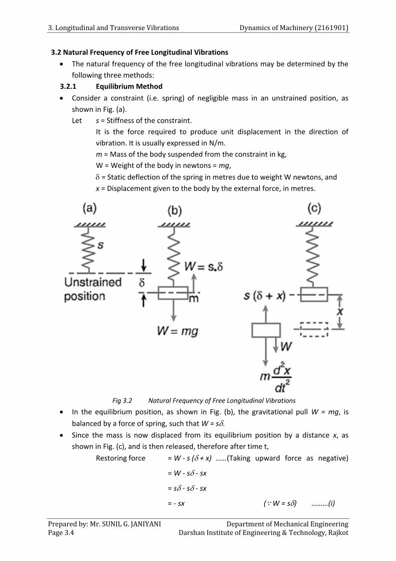
3. Longitudinal and Transverse Vibrations Dynamics of Machinery (2161901)
Prepared by: Mr. SUNIL G. JANIYANI Department of Mechanical Engineering Page 3.4 Darshan Institute of Engineering & Technology, Rajkot
3.2 Natural Frequency of Free Longitudinal Vibrations
The natural frequency of the free longitudinal vibrations may be determined by the
following three methods:
3.2.1 Equilibrium Method
Consider a constraint (i.e. spring) of negligible mass in an unstrained position, as
shown in Fig. (a).
Let s = Stiffness of the constraint.
It is the force required to produce unit displacement in the direction of
vibration. It is usually expressed in N/m.
m = Mass of the body suspended from the constraint in kg,
W = Weight of the body in newtons = mg,
= Static deflection of the spring in metres due to weight W newtons, and
x = Displacement given to the body by the external force, in metres.
Fig 3.2 Natural Frequency of Free Longitudinal Vibrations
In the equilibrium position, as shown in Fig. (b), the gravitational pull W = mg, is
balanced by a force of spring, such that W = s.
Since the mass is now displaced from its equilibrium position by a distance x, as
shown in Fig. (c), and is then released, therefore after time t,
Restoring force = W - s ( + x) ……(Taking upward force as negative)
= W - s - sx
= s - s - sx
= - sx (∵ W = s) ………(i)
Dynamics of Machinery (2161901) 3. Longitudinal and Transverse Vibrations
Department of Mechanical Engineering Prepared by: Mr. SUNIL G. JANIYANI Darshan Institute of Engineering & Technology, Rajkot Page 3.5
Accelerating force = Mass × Acceleration
= m × 𝑑2𝑥
𝑑𝑡2 ………(ii)
Equating equations (i) and (ii), the equation of motion of the body of mass m after
time t is
m × 𝑑2𝑥
𝑑𝑡2 = - s x
( m × 𝑑2𝑥
𝑑𝑡2 ) + s x = 0
𝑑2𝑥
𝑑𝑡2+ (
𝑠
𝑚 × 𝑥) = 0 ………(iii)
We know that the fundamental equation of simple harmonic motion is
𝑑2𝑥
𝑑𝑡2+ (𝜔2𝑥) = 0 ………(iv)
Comparing equations (iii) and (iv), we have
(𝑠
𝑚 × 𝑥) = (𝜔2𝑥)
𝜔 = √𝑠
𝑚
Time period, tp = 2 𝜋
𝜔= 2 𝜋√
𝑚
𝑠
Natural frequency, fn = 1
𝑡𝑝=
1
2 𝜋√
𝑠
𝑚 =
1
2 𝜋√
𝑔
𝛿 ……(∵ mg = s)
Taking the value of g as 9.81 m/s2 and in metres,
fn = 1
2 𝜋√
9.81
𝛿=
0.4985
√𝛿 Hz
3.2.2 Energy Method
We know that the kinetic energy is due to the motion of the body and the potential
energy is with respect to a certain datum position which is equal to the amount of
work required to move the body from the datum position.
In the case of vibrations, the datum position is the mean or equilibrium position at
which the potential energy of the body or the system is zero.
In the free vibrations, no energy is transferred to the system or from the system.
Therefore, the summation of kinetic energy and potential energy must be a constant
quantity which is same at all the times.
In other words, 𝑑
𝑑𝑡 (K.E. + P.E.) = 0
3. Longitudinal and Transverse Vibrations Dynamics of Machinery (2161901)
Prepared by: Mr. SUNIL G. JANIYANI Department of Mechanical Engineering Page 3.6 Darshan Institute of Engineering & Technology, Rajkot
We know that kinetic energy,
K.E. = 1
2 × 𝑚 (
𝑑𝑥
𝑑𝑡)
2
P.E. = Mean force x Displacement
= (0+𝑠 𝑥
2) 𝑥
= 1
2 × (𝑠 𝑥)2
∴𝑑
𝑑𝑡 [(
1
2× 𝑚 (
𝑑𝑥
𝑑𝑡)
2
) + (1
2 × (𝑠 𝑥)2)] = 0
∴ (1
2× 𝑚 × 2 ×
𝑑𝑥
𝑑𝑡×
𝑑2𝑥
𝑑𝑡2) + (
1
2 × 𝑠 × 2𝑥 ×
𝑑𝑥
𝑑𝑡) = 0
( m × 𝑑2𝑥
𝑑𝑡2 ) + s x = 0
𝑑2𝑥
𝑑𝑡2+ (
𝑠
𝑚 × 𝑥) = 0 ……… (Same as equilibrium method)
The time period and the natural frequency may be obtained as discussed in the
equilibrium method.
3.2.3 Rayleigh’s method
In this method, the maximum kinetic energy at the mean position is equal to the
maximum potential energy (or strain energy) at the extreme position.
Assuming the motion executed by the vibration to be simple harmonic, then
𝑥 = 𝑋 sin 𝜔𝑡 ………(i)
Where x = Displacement of the body from the mean position after time t seconds,
X = Maximum displacement from mean position to extreme position.
Now, differentiating equation (i), we have
𝑑𝑥
𝑑𝑡= 𝜔 𝑋 cos 𝜔𝑡
Since at the mean position, t = 0, therefore maximum velocity at the mean position,
𝑣 =𝑑𝑥
𝑑𝑡= 𝜔 𝑋
Maximum kinetic energy at mean position
=1
2× 𝑚 𝑣2
=1
2× 𝑚 𝜔2 𝑥2 ………(ii)
and maximum potential energy at the extreme position
= (0+𝑠 𝑥
2) 𝑥
= 1
2 × (𝑠 𝑥)2 ………(iii)
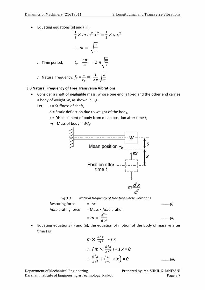
Dynamics of Machinery (2161901) 3. Longitudinal and Transverse Vibrations
Department of Mechanical Engineering Prepared by: Mr. SUNIL G. JANIYANI Darshan Institute of Engineering & Technology, Rajkot Page 3.7
Equating equations (ii) and (iii),
1
2× 𝑚 𝜔2 𝑥2 =
1
2× 𝑠 𝑥2
𝜔 = √𝑠
𝑚
Time period, tp = 2 𝜋
𝜔= 2 𝜋√
𝑚
𝑠
Natural frequency, fn = 1
𝑡𝑝=
1
2 𝜋√
𝑠
𝑚
3.3 Natural Frequency of Free Transverse Vibrations
Consider a shaft of negligible mass, whose one end is fixed and the other end carries
a body of weight W, as shown in Fig.
Let s = Stiffness of shaft,
= Static deflection due to weight of the body,
x = Displacement of body from mean position after time t,
m = Mass of body = W/g
Fig 3.3 Natural frequency of free transverse vibrations
Restoring force = - sx ………(i)
Accelerating force = Mass × Acceleration
= m × 𝑑2𝑥
𝑑𝑡2 ………(ii)
Equating equations (i) and (ii), the equation of motion of the body of mass m after
time t is
m × 𝑑2𝑥
𝑑𝑡2 = - s x
( m × 𝑑2𝑥
𝑑𝑡2 ) + s x = 0
𝑑2𝑥
𝑑𝑡2+ (
𝑠
𝑚 × 𝑥) = 0 ………(iii)
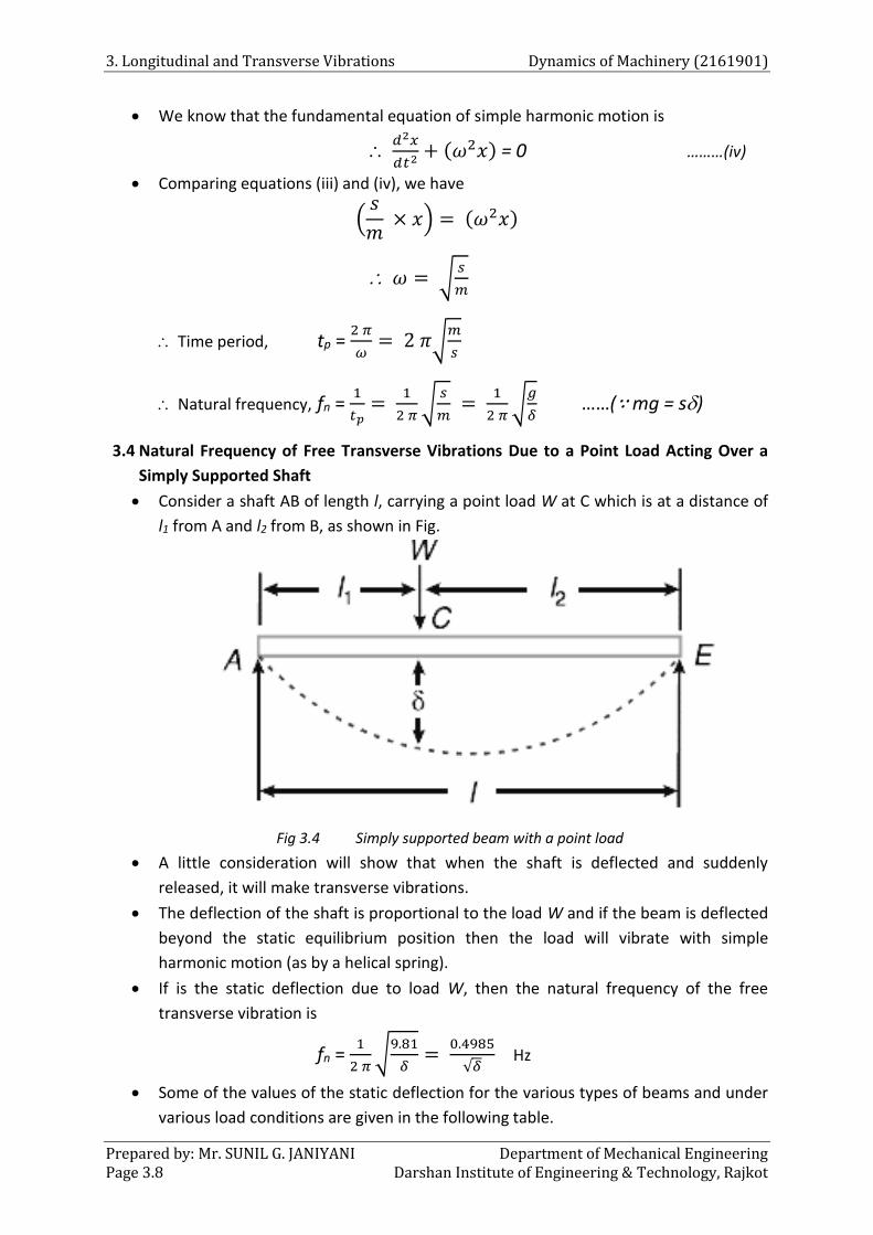
3. Longitudinal and Transverse Vibrations Dynamics of Machinery (2161901)
Prepared by: Mr. SUNIL G. JANIYANI Department of Mechanical Engineering Page 3.8 Darshan Institute of Engineering & Technology, Rajkot
We know that the fundamental equation of simple harmonic motion is
𝑑2𝑥
𝑑𝑡2+ (𝜔2𝑥) = 0 ………(iv)
Comparing equations (iii) and (iv), we have
(𝑠
𝑚 × 𝑥) = (𝜔2𝑥)
𝜔 = √𝑠
𝑚
Time period, tp = 2 𝜋
𝜔= 2 𝜋√
𝑚
𝑠
Natural frequency, fn = 1
𝑡𝑝=
1
2 𝜋√
𝑠
𝑚 =
1
2 𝜋√
𝑔
𝛿 ……(∵ mg = s)
3.4 Natural Frequency of Free Transverse Vibrations Due to a Point Load Acting Over a
Simply Supported Shaft
Consider a shaft AB of length l, carrying a point load W at C which is at a distance of
l1 from A and l2 from B, as shown in Fig.
Fig 3.4 Simply supported beam with a point load
A little consideration will show that when the shaft is deflected and suddenly
released, it will make transverse vibrations.
The deflection of the shaft is proportional to the load W and if the beam is deflected
beyond the static equilibrium position then the load will vibrate with simple
harmonic motion (as by a helical spring).
If is the static deflection due to load W, then the natural frequency of the free
transverse vibration is
fn = 1
2 𝜋√
9.81
𝛿=
0.4985
√𝛿 Hz
Some of the values of the static deflection for the various types of beams and under
various load conditions are given in the following table.
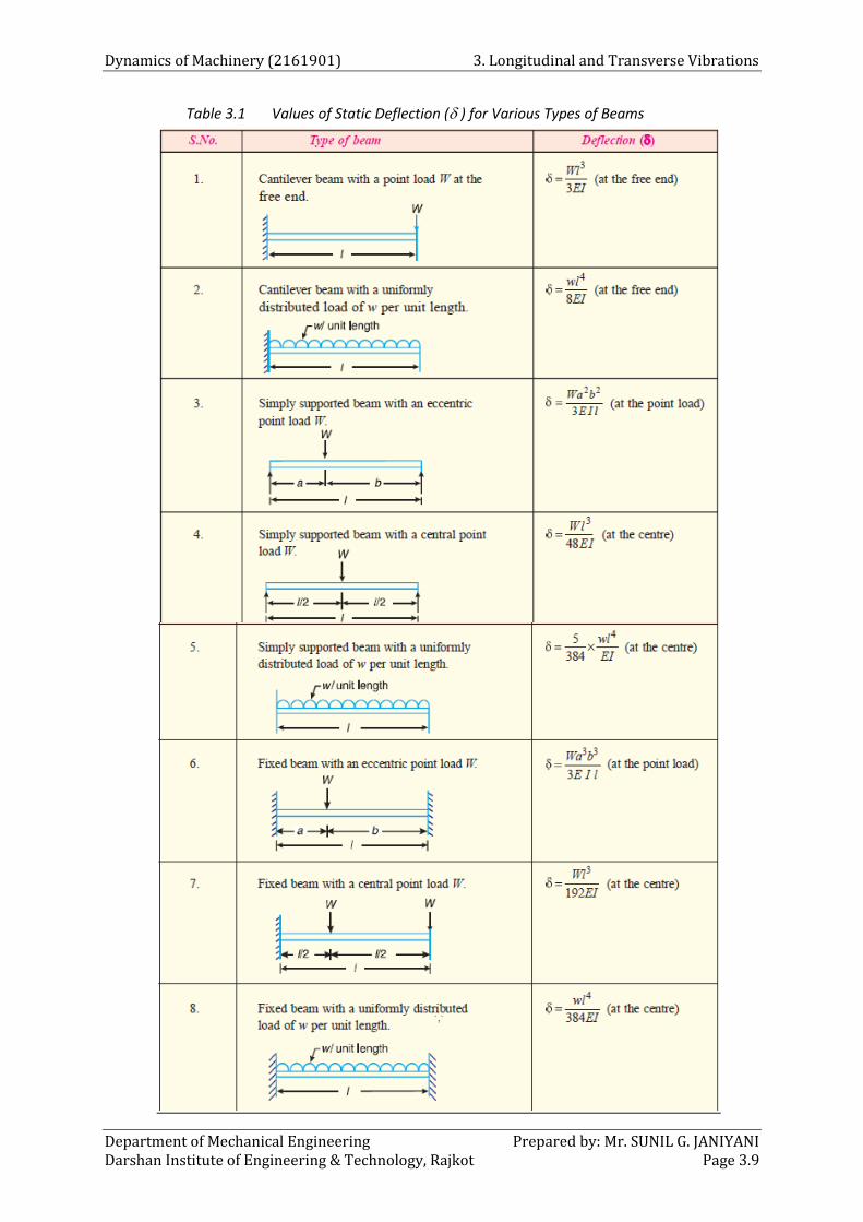
Dynamics of Machinery (2161901) 3. Longitudinal and Transverse Vibrations
Department of Mechanical Engineering Prepared by: Mr. SUNIL G. JANIYANI Darshan Institute of Engineering & Technology, Rajkot Page 3.9
Table 3.1 Values of Static Deflection ( ) for Various Types of Beams
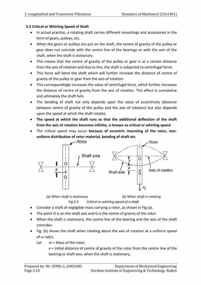
3. Longitudinal and Transverse Vibrations Dynamics of Machinery (2161901)
Prepared by: Mr. SUNIL G. JANIYANI Department of Mechanical Engineering Page 3.10 Darshan Institute of Engineering & Technology, Rajkot
3.5 Critical or Whirling Speed of Shaft
In actual practice, a rotating shaft carries different mountings and accessories in the
form of gears, pulleys, etc.
When the gears or pulleys are put on the shaft, the centre of gravity of the pulley or
gear does not coincide with the centre line of the bearings or with the axis of the
shaft, when the shaft is stationary.
This means that the centre of gravity of the pulley or gear is at a certain distance
from the axis of rotation and due to this, the shaft is subjected to centrifugal force.
This force will bend the shaft which will further increase the distance of centre of
gravity of the pulley or gear from the axis of rotation.
This correspondingly increases the value of centrifugal force, which further increases
the distance of centre of gravity from the axis of rotation. This effect is cumulative
and ultimately the shaft fails.
The bending of shaft not only depends upon the value of eccentricity (distance
between centre of gravity of the pulley and the axis of rotation) but also depends
upon the speed at which the shaft rotates.
The speed at which the shaft runs so that the additional deflection of the shaft
from the axis of rotation becomes infinite, is known as critical or whirling speed.
The critical speed may occur because of eccentric mounting of the rotor, non-
uniform distribution of rotor material, bending of shaft etc.
(a) When shaft is stationary (b) When shaft is rotating
Fig 3.5 Critical or whirling speed of a shaft
Consider a shaft of negligible mass carrying a rotor, as shown in Fig (a).
The point O is on the shaft axis and G is the centre of gravity of the rotor.
When the shaft is stationary, the centre line of the bearing and the axis of the shaft
coincides.
Fig. (b) shows the shaft when rotating about the axis of rotation at a uniform speed
of rad/s.
Let m = Mass of the rotor,
e = Initial distance of centre of gravity of the rotor from the centre line of the
bearing or shaft axis, when the shaft is stationary,
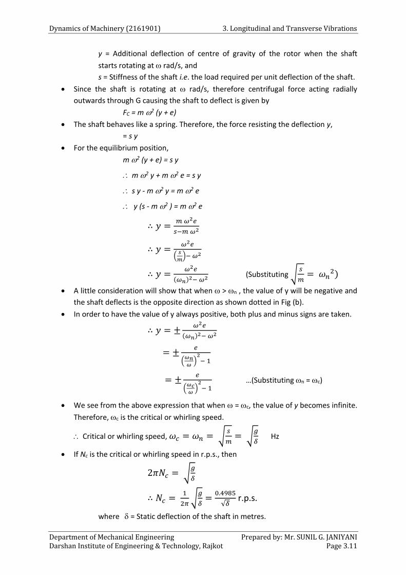
Dynamics of Machinery (2161901) 3. Longitudinal and Transverse Vibrations
Department of Mechanical Engineering Prepared by: Mr. SUNIL G. JANIYANI Darshan Institute of Engineering & Technology, Rajkot Page 3.11
y = Additional deflection of centre of gravity of the rotor when the shaft
starts rotating at rad/s, and
s = Stiffness of the shaft i.e. the load required per unit deflection of the shaft.
Since the shaft is rotating at rad/s, therefore centrifugal force acting radially
outwards through G causing the shaft to deflect is given by
FC = m 2 (y + e)
The shaft behaves like a spring. Therefore, the force resisting the deflection y,
= s y
For the equilibrium position,
m 2 (y + e) = s y
m 2 y + m 2 e = s y
s y - m 2 y = m 2 e
y (s - m 2 ) = m 2 e
∴ 𝑦 =𝑚 𝜔2𝑒
𝑠−𝑚 𝜔2
∴ 𝑦 =𝜔2𝑒
(𝑠
𝑚)− 𝜔2
∴ 𝑦 =𝜔2𝑒
(𝜔𝑛)2− 𝜔2 (Substituting √
𝑠
𝑚= 𝜔𝑛
2)
A little consideration will show that when > n , the value of y will be negative and
the shaft deflects is the opposite direction as shown dotted in Fig (b).
In order to have the value of y always positive, both plus and minus signs are taken.
∴ 𝑦 = ±𝜔2𝑒
(𝜔𝑛)2− 𝜔2
= ±𝑒
(𝜔𝑛𝜔
)2
− 1
= ±𝑒
(𝜔𝑐𝜔
)2
− 1 …(Substituting n = c)
We see from the above expression that when = c, the value of y becomes infinite.
Therefore, c is the critical or whirling speed.
Critical or whirling speed, 𝜔𝑐 = 𝜔𝑛 = √𝑠
𝑚= √
𝑔
𝛿 Hz
If Nc is the critical or whirling speed in r.p.s., then
2𝜋𝑁𝑐 = √𝑔
𝛿
∴ 𝑁𝑐 = 1
2𝜋√
𝑔
𝛿=
0.4985
√𝛿 r.p.s.
where = Static deflection of the shaft in metres.

3. Longitudinal and Transverse Vibrations Dynamics of Machinery (2161901)
Prepared by: Mr. SUNIL G. JANIYANI Department of Mechanical Engineering Page 3.12 Darshan Institute of Engineering & Technology, Rajkot
Hence the critical or whirling speed is the same as the natural frequency of
transverse vibration but its unit will be revolutions per second.
3.6 Frequency of Free Damped Vibrations (Viscous Damping)
We know that the motion of a body is resisted by frictional forces.
In vibrating systems, the effect of friction is referred to as damping.
The damping provided by fluid resistance is known as viscous damping.
We also know that in damped vibrations, the amplitude of the resulting vibration
gradually diminishes. This is due to the reason that a certain amount of energy is
always dissipated to overcome the frictional resistance.
The resistance to the motion of the body is provided partly by the medium in which
the vibration takes place and partly by the internal friction, and in some cases partly
by a dash pot or other external damping device.
Fig 3.6 Frequency of free damped vibrations
Consider a vibrating system, as shown in Fig., in which a mass is suspended from one
end of the spiral spring and the other end of which is fixed.
A damper is provided between the mass and the rigid support.
Let m = Mass suspended from the spring,
s = Stiffness of the spring,
x = Displacement of the mass from the mean position at time t,
= Static deflection of the spring = m.g/s, and
c = Damping coefficient or the damping force per unit velocity.
Since in viscous damping, it is assumed that the frictional resistance to the motion of
the body is directly proportional to the speed of the movement.
Therefore, damping force or frictional force on the mass acting in opposite direction
to the motion of the mass
= 𝑐 ×𝑑𝑥
𝑑𝑡
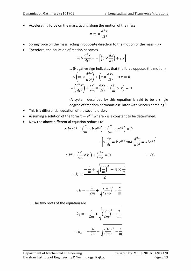
Dynamics of Machinery (2161901) 3. Longitudinal and Transverse Vibrations
Department of Mechanical Engineering Prepared by: Mr. SUNIL G. JANIYANI Darshan Institute of Engineering & Technology, Rajkot Page 3.13
Accelerating force on the mass, acting along the motion of the mass
= 𝑚 ×𝑑2𝑥
𝑑𝑡2
Spring force on the mass, acting in opposite direction to the motion of the mass = s x
Therefore, the equation of motion becomes
𝑚 ×𝑑2𝑥
𝑑𝑡2= − [(𝑐 ×
𝑑𝑥
𝑑𝑡) + 𝑠 𝑥]
… (Negative sign indicates that the force opposes the motion)
∴ (𝑚 ×𝑑2𝑥
𝑑𝑡2) + (𝑐 ×
𝑑𝑥
𝑑𝑡) + 𝑠 𝑥 = 0
∴ (𝑑2𝑥
𝑑𝑡2) + (
𝑐
𝑚×
𝑑𝑥
𝑑𝑡) + (
𝑠
𝑚 × 𝑥) = 0
(A system described by this equation is said to be a single
degree of freedom harmonic oscillator with viscous damping.)
This is a differential equation of the second order.
Assuming a solution of the form 𝑥 = 𝑒𝑘 𝑡 where k is a constant to be determined.
Now the above differential equation reduces to
∴ 𝑘2𝑒𝑘 𝑡 + (𝑐
𝑚× 𝑘 𝑒𝑘 𝑡) + (
𝑠
𝑚 × 𝑒𝑘 𝑡) = 0
… [∵𝑑𝑥
𝑑𝑡= 𝑘 𝑒𝑘 𝑡 𝑎𝑛𝑑
𝑑2𝑥
𝑑𝑡2= 𝑘2𝑒𝑘 𝑡]
∴ 𝑘2 + (𝑐
𝑚× 𝑘 ) + (
𝑠
𝑚) = 0 ⋯ (𝑖)
∴ 𝑘 =−
𝑐
𝑚± √(
𝑐
𝑚)
2− 4 ×
𝑠
𝑚
2
∴ 𝑘 = −𝑐
2𝑚± √(
𝑐
2𝑚)
2
−𝑠
𝑚
The two roots of the equation are
𝑘1 = −𝑐
2𝑚+ √(
𝑐
2𝑚)
2
−𝑠
𝑚
∴ 𝑘2 = −𝑐
2𝑚− √(
𝑐
2𝑚)
2
−𝑠
𝑚
3. Longitudinal and Transverse Vibrations Dynamics of Machinery (2161901)
Prepared by: Mr. SUNIL G. JANIYANI Department of Mechanical Engineering Page 3.14 Darshan Institute of Engineering & Technology, Rajkot
The most general solution of the differential equation (i) with its right hand side equal to
zero has only complementary function and it is given by
𝑥 = 𝐶1 𝑒(𝑘1 𝑡) + 𝐶2 𝑒(𝑘2 𝑡) ⋯ ⋯ ⋯ (𝑖𝑖)
where C1 and C2 are two arbitrary constants which are to be determined from
the initial conditions of the motion of the mass.
It may be noted that the roots k1 and k2 may be real, complex conjugate (imaginary) or
equal.
Let us now discuss these three cases as below:
1. When the roots are real (overdamping)
If (𝑐
2𝑚)
2
> 𝑠
𝑚, then roots k1 and k2 are real but negative.
This is a case of overdamping or large damping and the mass moves slowly to
the equilibrium position. This motion is known as aperiodic.
When the roots are real, the most general solution of the differential
equation is
𝑥 = 𝐶1 𝑒(𝑘1 𝑡) + 𝐶2 𝑒(𝑘2 𝑡)
∴ 𝑥 = 𝐶1 𝑒(−
𝑐
2𝑚+√(
𝑐
2𝑚)
2−
𝑠
𝑚)
+ 𝐶2 𝑒(−
𝑐
2𝑚−√(
𝑐
2𝑚)
2−
𝑠
𝑚)
Note: In actual practice, the overdamped vibrations are avoided.
2. When the roots are complex conjugate (underdamping)
If (𝑐
2𝑚)
2
< 𝑠
𝑚, then the radical (i.e. the term under the square root) becomes
negative.
The two roots k1 and k2 are then known as complex conjugate. This is a most
practical case of damping and it is known as underdamping or small damping.
The two roots are
𝑘1 = −𝑐
2𝑚+ 𝑖√
𝑠
𝑚− (
𝑐
2𝑚)
2
𝑘1 = −𝑐
2𝑚− 𝑖√
𝑠
𝑚− (
𝑐
2𝑚)
2
where i is a Greek letter known as iota and its value is √−1.
For the sake of mathematical calculations, let
𝑐
2𝑚= 𝑎 ;
𝑠
𝑚= (𝜔𝑛)2
Therefore, the two roots may be written as
𝑘1 = −𝑎 + 𝑖 𝜔𝑑 and 𝑘2 = −𝑎 − 𝑖 𝜔𝑑
Dynamics of Machinery (2161901) 3. Longitudinal and Transverse Vibrations
Department of Mechanical Engineering Prepared by: Mr. SUNIL G. JANIYANI Darshan Institute of Engineering & Technology, Rajkot Page 3.15
We know that the general solution of a differential equation is
𝑥 = 𝐶1 𝑒(𝑘1 𝑡) + 𝐶2 𝑒(𝑘2 𝑡)
∴ 𝑥 = 𝐶1 𝑒(−𝑎 + 𝑖 𝜔𝑑) 𝑡 + 𝐶2 𝑒(−𝑎 − 𝑖 𝜔𝑑) 𝑡
∴ 𝑥 = 𝑒−𝑎𝑡(𝐶1 𝑒 𝑖 𝜔𝑑𝑡 + 𝐶2 𝑒 − 𝑖 𝜔𝑑𝑡) ⋯ ⋯ ⋯ (𝑖𝑖𝑖)
Now according to Euler’s theorem
𝑒+𝑖 𝜃 = cos 𝜃 + 𝑖 sin 𝜃; 𝑎𝑛𝑑
𝑒−𝑖 𝜃 = cos 𝜃 − 𝑖 sin 𝜃
Therefore, the equation (iii) may be written as
𝑥 = 𝑒−𝑎𝑡[𝐶1 (cos 𝜔𝑑𝑡 + 𝑖 sin 𝜔𝑑𝑡) + 𝐶2(cos 𝜔𝑑𝑡 − 𝑖 sin 𝜔𝑑𝑡)]
∴ 𝑥 = 𝑒−𝑎𝑡[(𝐶1 + 𝐶2) cos 𝜔𝑑𝑡 + 𝑖 (𝐶1 − 𝐶2) sin 𝜔𝑑𝑡]
Let C1 + C2 = A, and i (C1 - C2) = B
∴ 𝑥 = 𝑒−𝑎𝑡[𝐴 cos 𝜔𝑑𝑡 + 𝐵 sin 𝜔𝑑𝑡]………(iv)
Again, let A = C cos , and B = C sin , therefore
𝐶 = √𝐴2 + 𝐵2
and tan 𝜃 = 𝐵
𝐴
Now the equation (iv) becomes
∴ 𝑥 = 𝑒−𝑎𝑡[C cos cos 𝜔𝑑𝑡 + C sin sin 𝜔𝑑𝑡]
∴ 𝑥 = 𝐶𝑒−𝑎𝑡(cos 𝜔𝑑𝑡 − )………(v)
If t is measured from the instant at which the mass m is released after an
initial displacement A, then
A = C cos … [Substituting x = A and t = 0 in equation (v)]
and when = 0, then A = C
The equation (v) may be written as
∴ 𝑥 = 𝐴 𝑒−𝑎𝑡(cos 𝜔𝑑𝑡)………(vi)
where 𝑐
2𝑚= 𝑎 ;
𝑠
𝑚= (𝜔𝑛)2
We see from equation (vi), that the motion of the mass is simple harmonic
whose circular damped frequency is d and the amplitude is A e-at which
diminishes exponentially with time as shown in below Fig.
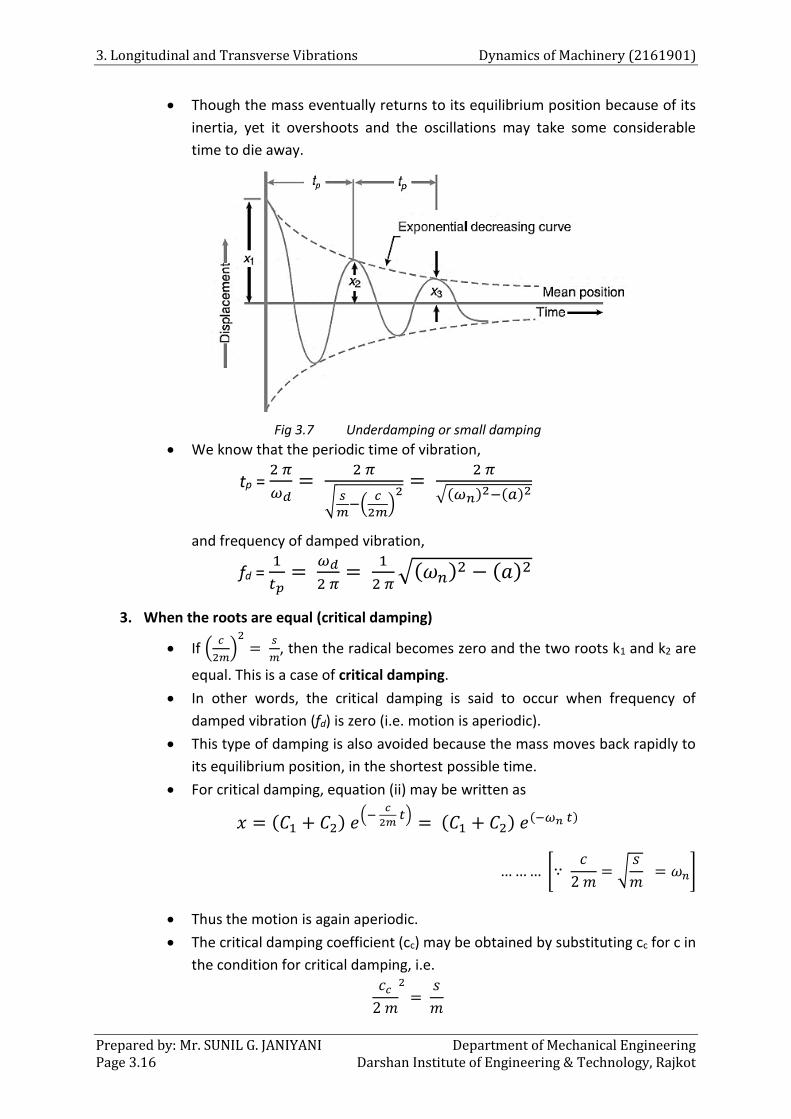
3. Longitudinal and Transverse Vibrations Dynamics of Machinery (2161901)
Prepared by: Mr. SUNIL G. JANIYANI Department of Mechanical Engineering Page 3.16 Darshan Institute of Engineering & Technology, Rajkot
Though the mass eventually returns to its equilibrium position because of its
inertia, yet it overshoots and the oscillations may take some considerable
time to die away.
Fig 3.7 Underdamping or small damping
We know that the periodic time of vibration,
tp = 2 𝜋
𝜔𝑑=
2 𝜋
√ 𝑠
𝑚−(
𝑐
2𝑚)
2=
2 𝜋
√(𝜔𝑛)2−(𝑎)2
and frequency of damped vibration,
fd = 1
𝑡𝑝=
𝜔𝑑
2 𝜋=
1
2 𝜋√(𝜔𝑛)2 − (𝑎)2
3. When the roots are equal (critical damping)
If (𝑐
2𝑚)
2
= 𝑠
𝑚, then the radical becomes zero and the two roots k1 and k2 are
equal. This is a case of critical damping.
In other words, the critical damping is said to occur when frequency of
damped vibration (fd) is zero (i.e. motion is aperiodic).
This type of damping is also avoided because the mass moves back rapidly to
its equilibrium position, in the shortest possible time.
For critical damping, equation (ii) may be written as
𝑥 = (𝐶1 + 𝐶2) 𝑒(−
𝑐
2𝑚 𝑡)
= (𝐶1 + 𝐶2) 𝑒(−𝜔𝑛 𝑡)
… … … [∵ 𝑐
2 𝑚= √
𝑠
𝑚 = 𝜔𝑛]
Thus the motion is again aperiodic.
The critical damping coefficient (cc) may be obtained by substituting cc for c in
the condition for critical damping, i.e.
𝑐𝑐
2 𝑚
2
= 𝑠
𝑚
Dynamics of Machinery (2161901) 3. Longitudinal and Transverse Vibrations
Department of Mechanical Engineering Prepared by: Mr. SUNIL G. JANIYANI Darshan Institute of Engineering & Technology, Rajkot Page 3.17
∴ 𝑐𝑐 = 2 𝑚 √𝑠
𝑚= 2 𝑚 𝜔𝑛
The critical damping coefficient is the amount of damping required for a
system to be critically damped.
3.7 Damping Factor or Damping Ratio
The ratio of the actual damping coefficient (c) to the critical damping coefficient (cc)
is known as damping factor or damping ratio.
Mathematically,
Damping factor = 𝑐
𝑐𝑐=
𝑐
2 𝑚 𝜔𝑛
The damping factor is the measure of the relative amount of damping in the existing
system with that necessary for the critical damped system.
3.8 Logarithmic decrement
It is defined as the natural logarithm of the amplitude reduction factor.
The amplitude reduction factor is the ratio of any two successive amplitudes on the
same side of the mean position.
If x1 and x2 are successive values of the amplitude on the same side of the mean
position (as shown in figure of underdamping) then amplitude reduction factor,
𝑥1
𝑥2=
𝐴 𝑒−𝑎𝑡
𝐴 𝑒−𝑎(𝑡 + 𝑡𝑝)= 𝑒𝑎 𝑡𝑝 = Constant
where tp is the period of forced oscillation or the time difference between two
consecutive amplitudes.
As per definition, logarithmic decrement,
𝛿 = 𝑙𝑜𝑔 (𝑥1
𝑥2) = 𝑙𝑜𝑔 𝑒𝑎 𝑡𝑝
∴ 𝛿 = 𝑙𝑜𝑔𝑒 (𝑥1
𝑥2) = 𝑎 𝑡𝑝 = 𝑎 ×
2 𝜋
𝜔𝑑=
𝑎 × 2 𝜋
√(𝜔𝑛)2 − (𝑎)2
∴ 𝛿 =
𝑐
2𝑚 × 2 𝜋
√(𝜔𝑛)2 − (𝑐
2𝑚)
2=
𝑐
2𝑚 × 2 𝜋
𝜔𝑛 √1 − (𝑐
2 𝑚 𝜔𝑛)
2
∴ 𝛿 = 𝑐 × 2 𝜋
𝑐𝑐 √1 − (𝑐
𝑐𝑐)
2 =
2 𝜋 𝑐
√(𝑐𝑐)2 − (𝑐)2
In general, amplitude reduction factor, 𝑥1
𝑥2=
𝑥2
𝑥3=
𝑥3
𝑥4= ⋯ ⋯ =
𝑥𝑛
𝑥𝑛+1= 𝑒𝑎 𝑡𝑝 = Constant
Logarithmic decrement,
∴ 𝛿 = 𝑙𝑜𝑔𝑒 (𝑥𝑛
𝑥𝑛+1) = 𝑎 𝑡𝑝 =
2 𝜋 𝑐
√(𝑐𝑐)2 − (𝑐)2
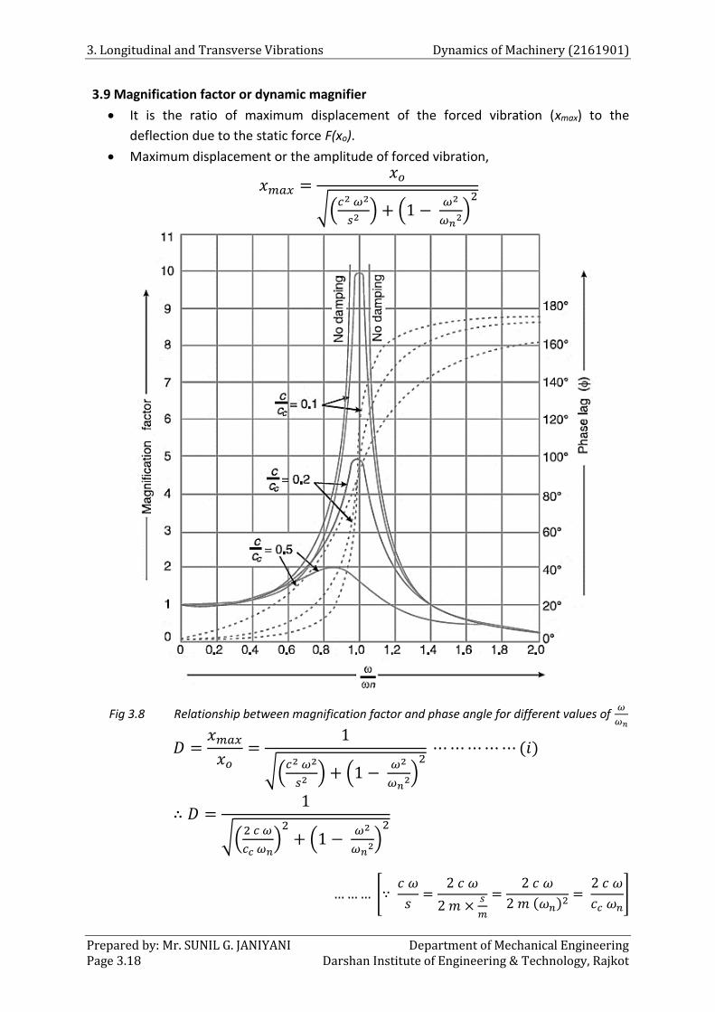
3. Longitudinal and Transverse Vibrations Dynamics of Machinery (2161901)
Prepared by: Mr. SUNIL G. JANIYANI Department of Mechanical Engineering Page 3.18 Darshan Institute of Engineering & Technology, Rajkot
3.9 Magnification factor or dynamic magnifier
It is the ratio of maximum displacement of the forced vibration (xmax) to the
deflection due to the static force F(xo).
Maximum displacement or the amplitude of forced vibration,
𝑥𝑚𝑎𝑥 =𝑥𝑜
√(𝑐2 𝜔2
𝑠2 ) + (1 − 𝜔2
𝜔𝑛2)
2
Fig 3.8 Relationship between magnification factor and phase angle for different values of 𝜔
𝜔𝑛
𝐷 =𝑥𝑚𝑎𝑥
𝑥𝑜=
1
√(𝑐2 𝜔2
𝑠2 ) + (1 − 𝜔2
𝜔𝑛2)
2 ⋯ ⋯ ⋯ ⋯ ⋯ (𝑖)
∴ 𝐷 =1
√(2 𝑐 𝜔
𝑐𝑐 𝜔𝑛)
2+ (1 −
𝜔2
𝜔𝑛2)
2
… … … [∵ 𝑐 𝜔
𝑠=
2 𝑐 𝜔
2 𝑚 ×𝑠
𝑚
=2 𝑐 𝜔
2 𝑚 (𝜔𝑛)2=
2 𝑐 𝜔
𝑐𝑐 𝜔𝑛]
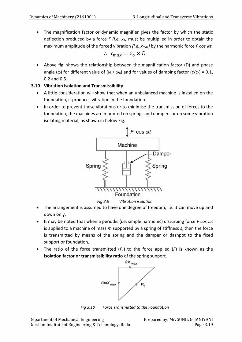
Dynamics of Machinery (2161901) 3. Longitudinal and Transverse Vibrations
Department of Mechanical Engineering Prepared by: Mr. SUNIL G. JANIYANI Darshan Institute of Engineering & Technology, Rajkot Page 3.19
The magnification factor or dynamic magnifier gives the factor by which the static
deflection produced by a force F (i.e. xo) must be multiplied in order to obtain the
maximum amplitude of the forced vibration (i.e. xmax) by the harmonic force F cos t
∴ 𝑥𝑚𝑎𝑥 = 𝑥𝑜 × 𝐷
Above fig. shows the relationship between the magnification factor (D) and phase
angle (φ) for different value of ( / n) and for values of damping factor (c/cc) = 0.1,
0.2 and 0.5.
3.10 Vibration isolation and Transmissibility
A little consideration will show that when an unbalanced machine is installed on the
foundation, it produces vibration in the foundation.
In order to prevent these vibrations or to minimise the transmission of forces to the
foundation, the machines are mounted on springs and dampers or on some vibration
isolating material, as shown in below Fig.
Fig 3.9 Vibration isolation
The arrangement is assumed to have one degree of freedom, i.e. it can move up and
down only.
It may be noted that when a periodic (i.e. simple harmonic) disturbing force F cos t
is applied to a machine of mass m supported by a spring of stiffness s, then the force
is transmitted by means of the spring and the damper or dashpot to the fixed
support or foundation.
The ratio of the force transmitted (FT) to the force applied (F) is known as the
isolation factor or transmissibility ratio of the spring support.
Fig 3.10 Force Transmitted to the Foundation
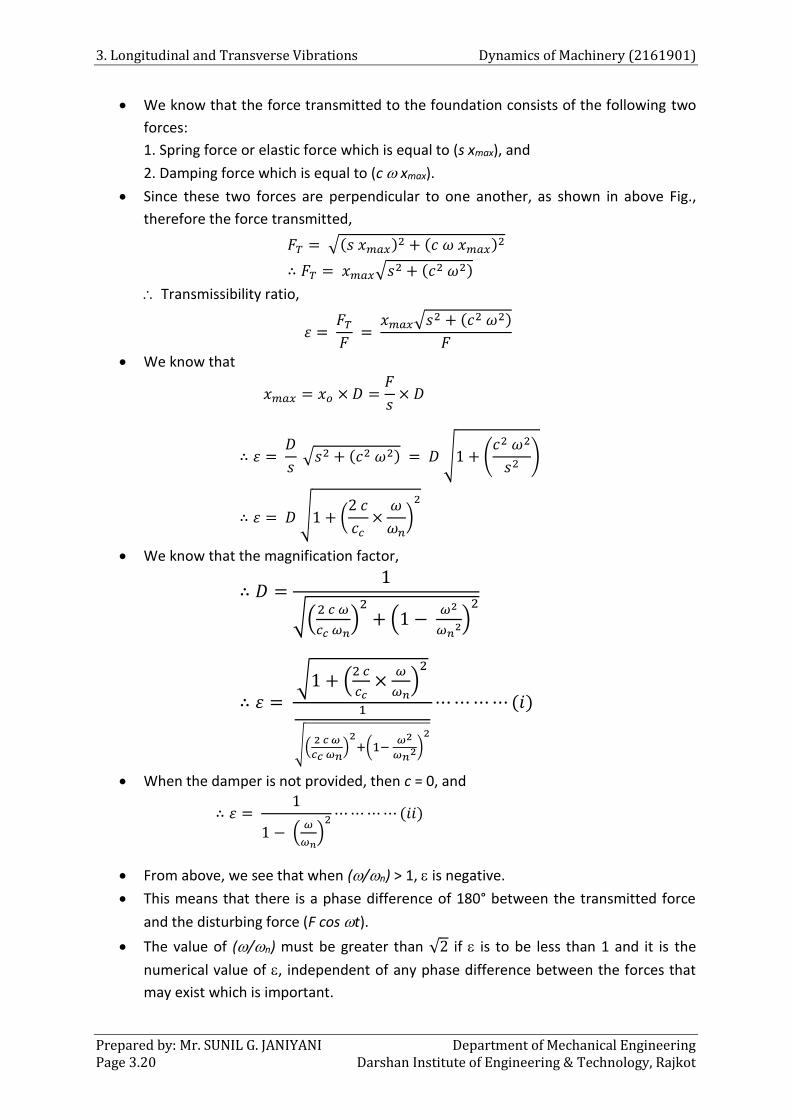
3. Longitudinal and Transverse Vibrations Dynamics of Machinery (2161901)
Prepared by: Mr. SUNIL G. JANIYANI Department of Mechanical Engineering Page 3.20 Darshan Institute of Engineering & Technology, Rajkot
We know that the force transmitted to the foundation consists of the following two
forces:
1. Spring force or elastic force which is equal to (s xmax), and
2. Damping force which is equal to (c xmax).
Since these two forces are perpendicular to one another, as shown in above Fig.,
therefore the force transmitted,
𝐹𝑇 = √(𝑠 𝑥𝑚𝑎𝑥)2 + (𝑐 𝜔 𝑥𝑚𝑎𝑥)2
∴ 𝐹𝑇 = 𝑥𝑚𝑎𝑥√𝑠2 + (𝑐2 𝜔2)
Transmissibility ratio,
휀 = 𝐹𝑇
𝐹 =
𝑥𝑚𝑎𝑥√𝑠2 + (𝑐2 𝜔2)
𝐹
We know that
𝑥𝑚𝑎𝑥 = 𝑥𝑜 × 𝐷 =𝐹
𝑠× 𝐷
∴ 휀 = 𝐷
𝑠 √𝑠2 + (𝑐2 𝜔2) = 𝐷 √1 + (
𝑐2 𝜔2
𝑠2)
∴ 휀 = 𝐷 √1 + (2 𝑐
𝑐𝑐×
𝜔
𝜔𝑛)
2
We know that the magnification factor,
∴ 𝐷 =1
√(2 𝑐 𝜔
𝑐𝑐 𝜔𝑛)
2+ (1 −
𝜔2
𝜔𝑛2)
2
∴ 휀 = √1 + (
2 𝑐
𝑐𝑐×
𝜔
𝜔𝑛)
2
1
√(2 𝑐 𝜔
𝑐𝑐 𝜔𝑛)
2+(1−
𝜔2
𝜔𝑛2)
2
⋯ ⋯ ⋯ ⋯ (𝑖)
When the damper is not provided, then c = 0, and
∴ 휀 = 1
1 − (𝜔
𝜔𝑛)
2 ⋯ ⋯ ⋯ ⋯ (𝑖𝑖)
From above, we see that when (/n) > 1, is negative.
This means that there is a phase difference of 180° between the transmitted force
and the disturbing force (F cos t).
The value of (/n) must be greater than √2 if is to be less than 1 and it is the
numerical value of , independent of any phase difference between the forces that
may exist which is important.
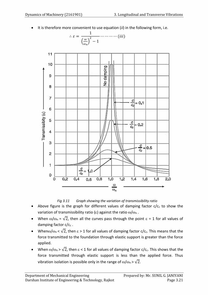
Dynamics of Machinery (2161901) 3. Longitudinal and Transverse Vibrations
Department of Mechanical Engineering Prepared by: Mr. SUNIL G. JANIYANI Darshan Institute of Engineering & Technology, Rajkot Page 3.21
It is therefore more convenient to use equation (ii) in the following form, i.e.
∴ 휀 = 1
(𝜔
𝜔𝑛)
2
− 1 ⋯ ⋯ ⋯ ⋯ (𝑖𝑖𝑖)
Fig 3.11 Graph showing the variation of transmissibility ratio
Above figure is the graph for different values of damping factor c/cc to show the
variation of transmissibility ratio () against the ratio /n .
When /n = √2, then all the curves pass through the point = 1 for all values of
damping factor c/cc .
When/n < √2, then > 1 for all values of damping factor c/cc. This means that the
force transmitted to the foundation through elastic support is greater than the force
applied.
When /n > √2, then < 1 for all values of damping factor c/cc. This shows that the
force transmitted through elastic support is less than the applied force. Thus
vibration isolation is possible only in the range of /n > √2.
3. Longitudinal and Transverse Vibrations Dynamics of Machinery (2161901)
Prepared by: Mr. SUNIL G. JANIYANI Department of Mechanical Engineering Page 3.22 Darshan Institute of Engineering & Technology, Rajkot
We also see from the curves in the above figure that the damping is detrimental
beyond /n > √2 and advantageous only in the region /n < √2 .
It is thus concluded that for the vibration isolation, dampers need not to be provided
but in order to limit resonance amplitude, stops may be provided.
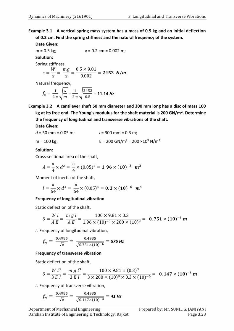
Dynamics of Machinery (2161901) 3. Longitudinal and Transverse Vibrations
Department of Mechanical Engineering Prepared by: Mr. SUNIL G. JANIYANI Darshan Institute of Engineering & Technology, Rajkot Page 3.23
Example 3.1 A vertical spring mass system has a mass of 0.5 kg and an initial deflection
of 0.2 cm. Find the spring stiffness and the natural frequency of the system.
Date Given:
m = 0.5 kg; x = 0.2 cm = 0.002 m;
Solution:
Spring stiffness,
𝑠 =𝑊
𝑥=
𝑚𝑔
𝑥=
0.5 × 9.81
0.002= 𝟐𝟒𝟓𝟐 𝑵/𝒎
Natural frequency,
fn = 1
2 𝜋√
𝑠
𝑚 =
1
2 𝜋√
2452
0.5 = 11.14 Hz
Example 3.2 A cantilever shaft 50 mm diameter and 300 mm long has a disc of mass 100
kg at its free end. The Young's modulus for the shaft material is 200 GN/m2. Determine
the frequency of longitudinal and transverse vibrations of the shaft.
Date Given:
d = 50 mm = 0.05 m; l = 300 mm = 0.3 m;
m = 100 kg; E = 200 GN/m2 = 200 ×109 N/m2
Solution:
Cross-sectional area of the shaft,
𝐴 =𝜋
4× 𝑑2 =
𝜋
4× (0.05)2 = 𝟏. 𝟗𝟔 × (𝟏𝟎)−𝟑 𝒎𝟐
Moment of inertia of the shaft,
𝐼 =𝜋
64× 𝑑4 =
𝜋
64× (0.05)4 = 𝟎. 𝟑 × (𝟏𝟎)−𝟔 𝒎𝟒
Frequency of longitudinal vibration
Static deflection of the shaft,
𝛿 =𝑊 𝑙
𝐴 𝐸=
𝑚 𝑔 𝑙
𝐴 𝐸=
100 × 9.81 × 0.3
1.96 × (10)−3 × 200 × (10)9= 𝟎. 𝟕𝟓𝟏 × (𝟏𝟎)−𝟔 𝒎
Frequency of longitudinal vibration,
𝑓𝑛 = 0.4985
√𝛿=
0.4985
√0.751×(10)−6= 575 Hz
Frequency of transverse vibration
Static deflection of the shaft,
𝛿 =𝑊 𝑙3
3 𝐸 𝐼=
𝑚 𝑔 𝑙3
3 𝐸 𝐼=
100 × 9.81 × (0.3)3
3 × 200 × (10)9 × 0.3 × (10)−6= 𝟎. 𝟏𝟒𝟕 × (𝟏𝟎)−𝟑 𝒎
Frequency of transverse vibration,
𝑓𝑛 = 0.4985
√𝛿=
0.4985
√0.147×(10)−3= 41 Hz
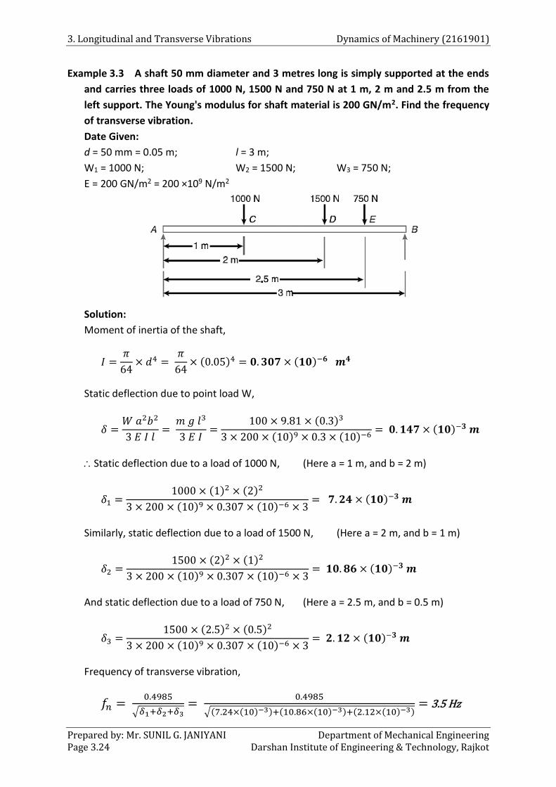
3. Longitudinal and Transverse Vibrations Dynamics of Machinery (2161901)
Prepared by: Mr. SUNIL G. JANIYANI Department of Mechanical Engineering Page 3.24 Darshan Institute of Engineering & Technology, Rajkot
Example 3.3 A shaft 50 mm diameter and 3 metres long is simply supported at the ends
and carries three loads of 1000 N, 1500 N and 750 N at 1 m, 2 m and 2.5 m from the
left support. The Young's modulus for shaft material is 200 GN/m2. Find the frequency
of transverse vibration.
Date Given:
d = 50 mm = 0.05 m; l = 3 m;
W1 = 1000 N; W2 = 1500 N; W3 = 750 N;
E = 200 GN/m2 = 200 ×109 N/m2
Solution:
Moment of inertia of the shaft,
𝐼 =𝜋
64× 𝑑4 =
𝜋
64× (0.05)4 = 𝟎. 𝟑𝟎𝟕 × (𝟏𝟎)−𝟔 𝒎𝟒
Static deflection due to point load W,
𝛿 =𝑊 𝑎2𝑏2
3 𝐸 𝐼 𝑙=
𝑚 𝑔 𝑙3
3 𝐸 𝐼=
100 × 9.81 × (0.3)3
3 × 200 × (10)9 × 0.3 × (10)−6= 𝟎. 𝟏𝟒𝟕 × (𝟏𝟎)−𝟑 𝒎
Static deflection due to a load of 1000 N, (Here a = 1 m, and b = 2 m)
𝛿1 =1000 × (1)2 × (2)2
3 × 200 × (10)9 × 0.307 × (10)−6 × 3= 𝟕. 𝟐𝟒 × (𝟏𝟎)−𝟑 𝒎
Similarly, static deflection due to a load of 1500 N, (Here a = 2 m, and b = 1 m)
𝛿2 =1500 × (2)2 × (1)2
3 × 200 × (10)9 × 0.307 × (10)−6 × 3= 𝟏𝟎. 𝟖𝟔 × (𝟏𝟎)−𝟑 𝒎
And static deflection due to a load of 750 N, (Here a = 2.5 m, and b = 0.5 m)
𝛿3 =1500 × (2.5)2 × (0.5)2
3 × 200 × (10)9 × 0.307 × (10)−6 × 3= 𝟐. 𝟏𝟐 × (𝟏𝟎)−𝟑 𝒎
Frequency of transverse vibration,
𝑓𝑛 = 0.4985
√𝛿1+𝛿2+𝛿3=
0.4985
√(7.24×(10)−3)+(10.86×(10)−3)+(2.12×(10)−3)= 3.5 Hz
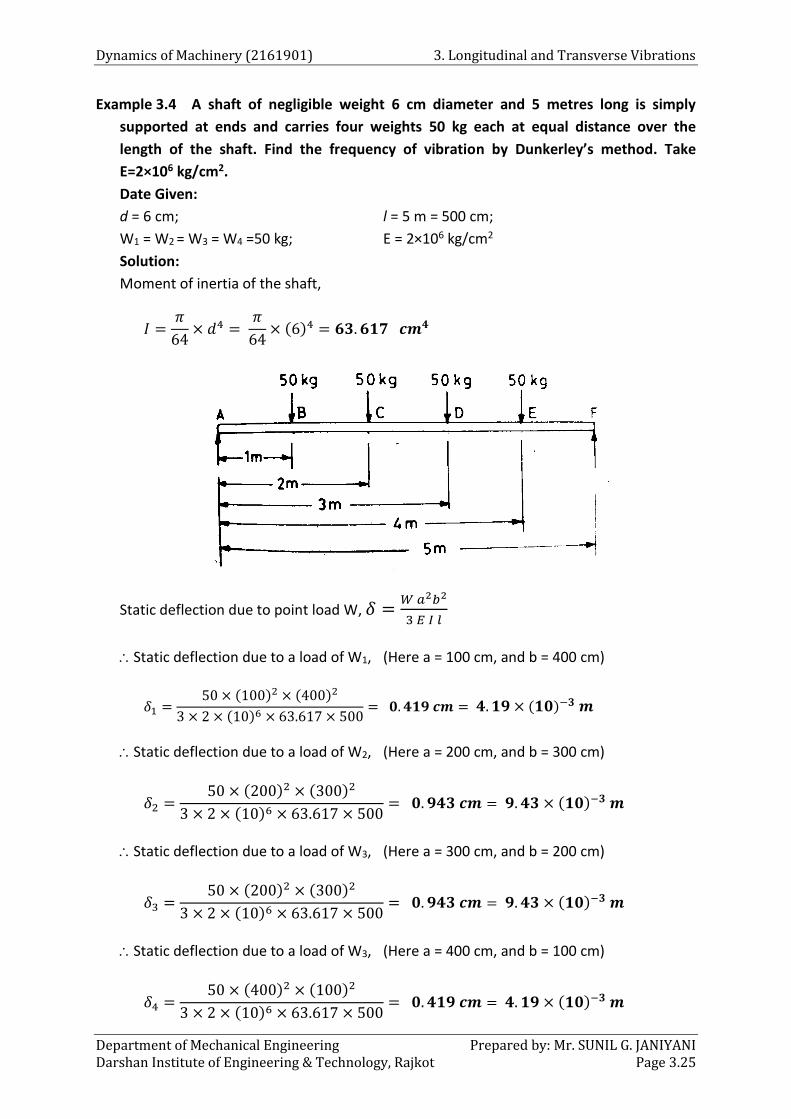
Dynamics of Machinery (2161901) 3. Longitudinal and Transverse Vibrations
Department of Mechanical Engineering Prepared by: Mr. SUNIL G. JANIYANI Darshan Institute of Engineering & Technology, Rajkot Page 3.25
Example 3.4 A shaft of negligible weight 6 cm diameter and 5 metres long is simply
supported at ends and carries four weights 50 kg each at equal distance over the
length of the shaft. Find the frequency of vibration by Dunkerley’s method. Take
E=2×10⁶ kg/cm2.
Date Given:
d = 6 cm; l = 5 m = 500 cm;
W1 = W2 = W3 = W4 =50 kg; E = 2×10⁶ kg/cm2
Solution:
Moment of inertia of the shaft,
𝐼 =𝜋
64× 𝑑4 =
𝜋
64× (6)4 = 𝟔𝟑. 𝟔𝟏𝟕 𝒄𝒎𝟒
Static deflection due to point load W, 𝛿 =𝑊 𝑎2𝑏2
3 𝐸 𝐼 𝑙
Static deflection due to a load of W1, (Here a = 100 cm, and b = 400 cm)
𝛿1 =50 × (100)2 × (400)2
3 × 2 × (10)6 × 63.617 × 500= 𝟎. 𝟒𝟏𝟗 𝒄𝒎 = 𝟒. 𝟏𝟗 × (𝟏𝟎)−𝟑 𝒎
Static deflection due to a load of W2, (Here a = 200 cm, and b = 300 cm)
𝛿2 =50 × (200)2 × (300)2
3 × 2 × (10)6 × 63.617 × 500= 𝟎. 𝟗𝟒𝟑 𝒄𝒎 = 𝟗. 𝟒𝟑 × (𝟏𝟎)−𝟑 𝒎
Static deflection due to a load of W3, (Here a = 300 cm, and b = 200 cm)
𝛿3 =50 × (200)2 × (300)2
3 × 2 × (10)6 × 63.617 × 500= 𝟎. 𝟗𝟒𝟑 𝒄𝒎 = 𝟗. 𝟒𝟑 × (𝟏𝟎)−𝟑 𝒎
Static deflection due to a load of W3, (Here a = 400 cm, and b = 100 cm)
𝛿4 =50 × (400)2 × (100)2
3 × 2 × (10)6 × 63.617 × 500= 𝟎. 𝟒𝟏𝟗 𝒄𝒎 = 𝟒. 𝟏𝟗 × (𝟏𝟎)−𝟑 𝒎
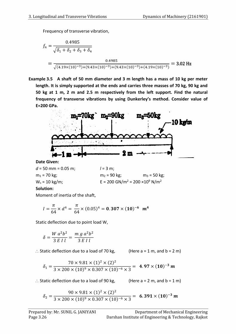
3. Longitudinal and Transverse Vibrations Dynamics of Machinery (2161901)
Prepared by: Mr. SUNIL G. JANIYANI Department of Mechanical Engineering Page 3.26 Darshan Institute of Engineering & Technology, Rajkot
Frequency of transverse vibration,
𝑓𝑛 =0.4985
√𝛿1 + 𝛿2 + 𝛿3 + 𝛿4
=0.4985
√(4.19×(10)−3)+(9.43×(10)−3)+(9.43×(10)−3)+(4.19×(10)−3)= 3.02 Hz
Example 3.5 A shaft of 50 mm diameter and 3 m length has a mass of 10 kg per meter
length. It is simply supported at the ends and carries three masses of 70 kg, 90 kg and
50 kg at 1 m, 2 m and 2.5 m respectively from the left support. Find the natural
frequency of transverse vibrations by using Dunkerley’s method. Consider value of
E=200 GPa.
Date Given:
d = 50 mm = 0.05 m; l = 3 m;
m1 = 70 kg; m2 = 90 kg; m3 = 50 kg;
Ws = 10 kg/m; E = 200 GN/m2 = 200 ×109 N/m2
Solution:
Moment of inertia of the shaft,
𝐼 =𝜋
64× 𝑑4 =
𝜋
64× (0.05)4 = 𝟎. 𝟑𝟎𝟕 × (𝟏𝟎)−𝟔 𝒎𝟒
Static deflection due to point load W,
𝛿 =𝑊 𝑎2𝑏2
3 𝐸 𝐼 𝑙=
𝑚 𝑔 𝑎2𝑏2
3 𝐸 𝐼 𝑙
Static deflection due to a load of 70 kg, (Here a = 1 m, and b = 2 m)
𝛿1 =70 × 9.81 × (1)2 × (2)2
3 × 200 × (10)9 × 0.307 × (10)−6 × 3= 𝟒. 𝟗𝟕 × (𝟏𝟎)−𝟑 𝒎
Static deflection due to a load of 90 kg, (Here a = 2 m, and b = 1 m)
𝛿2 =90 × 9.81 × (1)2 × (2)2
3 × 200 × (10)9 × 0.307 × (10)−6 × 3= 𝟔. 𝟑𝟗𝟏 × (𝟏𝟎)−𝟑 𝒎
Dynamics of Machinery (2161901) 3. Longitudinal and Transverse Vibrations
Department of Mechanical Engineering Prepared by: Mr. SUNIL G. JANIYANI Darshan Institute of Engineering & Technology, Rajkot Page 3.27
Static deflection due to a load of 50 kg, (Here a = 2.5 m, and b = 0.5 m)
𝛿3 =50 × 9.81 × (2.5)2 × (0.5)2
3 × 200 × (10)9 × 0.307 × (10)−6 × 3= 𝟏. 𝟑𝟖𝟕 × (𝟏𝟎)−𝟑 𝒎
Static deflection due to self-weight,
𝛿𝑠 =5 𝑚 𝑔 𝑙4
384 𝐸 𝐼=
5 × 10 × 9.81 × (3)4
384 × 200 × (10)9 × 0.307 × (10)−6= 𝟏. 𝟔𝟖𝟓 × (𝟏𝟎)−𝟑 𝒎
Frequency of transverse vibration,
𝑓𝑛 = 0.4985
√𝛿1 + 𝛿2 + 𝛿3 +𝛿𝑠
1.27
= 0.4985
√(4.97×(10)−3)+(6.391×(10)−3)+(1.387×(10)−3)+(1.985×(10)−3)
1.27
= 4.202 Hz
Example 3.6 A horizontal shaft of 10 mm diameter is simply supported at both ends by
bearings. A rotor of mass 5 Kg is attached at middle of the horizontal shaft. The span
between two bearings is 500 mm. The center gravity of the rotor is 2.5 mm offset from
the geometric center of the rotor. Find the deflection of the shaft and critical speed of
the shaft.
Date Given:
m = 5 kg; d = 10 mm = 0.01 m; l = 500 mm = 0.5 m;
e = 2.5 mm = 2.5 ×10 -3 m
Assume, E = 200 GN/m2 = 200 ×109 N/m2
Solution:
Moment of inertia of the shaft,
𝐼 =𝜋
64× 𝑑4 =
𝜋
64× (0.01)4 = 𝟎. 𝟒𝟗𝟏 × (𝟏𝟎)−𝟗 𝒎𝟒
Static deflection of the shaft, (Shaft to be freely supported)
𝛿 =𝑊 𝑙3
48 𝐸 𝐼=
𝑚 𝑔 𝑙3
48 𝐸 𝐼=
5 × 9.81 × (0.5)3
48 × 200 × (10)9 × 0.491 × (10)−9= 𝟏. 𝟑 × (𝟏𝟎)−𝟑 𝒎
Frequency of transverse vibration,
𝑓𝑛 = 0.4985
√𝛿=
0.4985
√1.3×(10)−3= 13.82 Hz
Critical speed of a shaft in r.p.s. is equal to the frequency of transverse vibration in Hz,
Nc = 13.82 r.p.s. = 13.82 × 60 = 829.2 r.p.m.
3. Longitudinal and Transverse Vibrations Dynamics of Machinery (2161901)
Prepared by: Mr. SUNIL G. JANIYANI Department of Mechanical Engineering Page 3.28 Darshan Institute of Engineering & Technology, Rajkot
Example 3.7 A rotor has a mass of 12 kg and is mounted on the middle of 24 mm
diameter horizontal shaft supported at two bearings. The length of the shaft is 1 m.
The shaft rotates at 2400 rpm. If the center of mass of the rotor is 0.11 mm eccentric
to the geometric center of the rotor. Find the amplitude of steady state vibration and
dynamic force transmitted to bearings. E=200 GN/m2. Assume the shaft to be freely
supported. Assume the shaft to be massless.
Date Given:
m = 12 kg; d = 24 mm = 0.024 m;
l = 1 m; N = 2400 rpm
e = 0.11 mm = 0.11 ×10 -3 m E = 200 GN/m2 = 200 ×109 N/m2
Solution:
Moment of inertia of the shaft,
𝐼 =𝜋
64× 𝑑4 =
𝜋
64× (0.024)4 = 𝟏𝟔. 𝟑 × (𝟏𝟎)−𝟗 𝒎𝟒
Static deflection of the shaft, (Shaft to be freely supported)
𝛿 =𝑊 𝑙3
48 𝐸 𝐼=
𝑚 𝑔 𝑙3
48 𝐸 𝐼=
12 × 9.81 × (1)3
48 × 200 × (10)9 × 16.3 × (10)−9= 𝟎. 𝟕𝟓𝟐 × (𝟏𝟎)−𝟑 𝒎
Frequency of transverse vibration,
𝑓𝑛 = 0.4985
√𝛿=
0.4985
√0.752×(10)−3= 18.17 Hz
Critical speed of a shaft in r.p.s. is equal to the frequency of transverse vibration in Hz,
Nc = 18.17 r.p.s. = 18.17 × 60 = 1090 r.p.m.
Amplitude,
𝑦 = ± 𝑒
(𝑁𝑐𝑁
)2
−1=
± 0.11×(10)−3
(1090
2400)
2−1
= 0.139 ×10 -3 m
Dynamic force on the bearings = 𝑚 𝑦 𝜔𝑐2 = 𝑚 𝑦 (
2 𝜋 𝑁𝑐
60)
2
= 12 × 0.139 × (10)−3 (2 × 𝜋 × 1090
60)
2
= 𝟐𝟏. 𝟕𝟑 𝑵
Example 3.8 The following data refers to a shaft held in long bearings.
Length and diameter of shaft is 1.2 m and 14 mm respectively.
Mass of the rotor at midpoint = 16 Kg,
Eccentricity of center of mass of rotor from center of rotor = 0.4 mm,
Modulus of rigidity of shaft material = 200 GN/m2,
Permissible stress in the shaft material = 70 x 106 N/m2.
Determine the critical speed of the shaft and the range of speed over which it is unsafe
to run the shaft. Assume the shaft to be fixed at both ends. Assume the shaft to be
massless.
Dynamics of Machinery (2161901) 3. Longitudinal and Transverse Vibrations
Department of Mechanical Engineering Prepared by: Mr. SUNIL G. JANIYANI Darshan Institute of Engineering & Technology, Rajkot Page 3.29
Date Given:
l = 1.2 m; d = 14 mm = 0.014 m; m = 16 kg; e = 0.4 mm = 0.4 ×10 -3 m E = 200 GN/m2 = 200 ×109 N/m2 σ = 70 ×106 N/m2 Solution:
Moment of inertia of the shaft,
𝐼 =𝜋
64× 𝑑4 =
𝜋
64× (0.014)4 = 𝟏. 𝟖𝟖𝟔 × (𝟏𝟎)−𝟗 𝒎𝟒
Static deflection of the shaft, (Shaft to be fixed at both ends)
𝛿 =𝑊 𝑙3
192 𝐸 𝐼=
𝑚 𝑔 𝑙3
192 𝐸 𝐼=
16 × 9.81 × (1.2)3
192 × 200 × (10)9 × 1.886 × (10)−9= 𝟑. 𝟕𝟓 × (𝟏𝟎)−𝟑 𝒎
Frequency of transverse vibration,
𝑓𝑛 = 0.4985
√𝛿=
0.4985
√3.75×(10)−3= 8.146 Hz
Critical speed of a shaft in r.p.s. is equal to the frequency of transverse vibration in Hz,
Nc = 8.146 r.p.s. = 8.146 × 60 = 489 r.p.m.
When the shaft starts rotating, the additional dynamic load (W1) to which the shaft is
subjected, may be obtained by using the bending equation, 𝑀
𝐼=
𝜎
𝑦1
For a shaft fixed at both ends and carrying a point load (W1) at the centre, the maximum
bending moment,
𝑀 =𝑊1𝑙
8
∴(
𝑊1𝑙
8)
𝐼=
𝜎
𝑑/2
∴ 𝑊1 =8 𝜎 𝐼
𝑙 ×𝑑
2
=8 × 70 × (10)6 × 1.886 × (10)−9
1.2 ×0.014
2
= 𝟏𝟐𝟓. 𝟕 𝑵
Additional deflection due to load W1,
𝑦 =𝑊1
𝑊× 𝛿 =
𝑊1
𝑚𝑔× 𝛿 =
125.7
16 × 9.81× 3.75 × (10)−3 = 𝟎. 𝟎𝟎𝟑 𝒎
Amplitude or Additional deflection,
𝑦 = ± 𝑒
(𝑁𝑐𝑁
)2
−1
∴ 0.003 = ± 0.4×(10)−3
(489
𝑁)
2−1
3. Longitudinal and Transverse Vibrations Dynamics of Machinery (2161901)
Prepared by: Mr. SUNIL G. JANIYANI Department of Mechanical Engineering Page 3.30 Darshan Institute of Engineering & Technology, Rajkot
∴ (489
𝑁)
2− 1 =
± 0.4×(10)−3
0.003
∴ (489
𝑁)
2
− 1 = ± 0.1333
∴ (489
𝑁)
2= 1.1333 𝑜𝑟 0.8667
∴489
𝑁= √1.1333 𝑜𝑟 √0.8667
∴ 𝑁1 =489
√1.1333 & 𝑁2 =
489
√0.8667
∴ 𝑵𝟏 = 𝟒𝟓𝟗 𝒓𝒑𝒎 & 𝑵𝟐 = 𝟓𝟐𝟓 𝒓𝒑𝒎
Example 3.9 A gun barrel of mass 600 Kg has a recoil spring of stiffness 294 KN/m. If the
barrel recoils 1.3 meter on firing, determine, (i) the initial recoil velocity of the barrel &
(ii) the critical damping coefficient of the dashpot which is engaged at the end of the
recoil stroke.
Date Given:
m = 600 kg; s = 294 KN/m = 294000 N/m; x = 1.3 m;
Solution:
Recoil velocity of the barrel K. E. of the barrel = P. E. of the spring
1
2× 𝑚 × 𝑣2 =
1
2× 𝑠 × 𝑥2
∴1
2× 600 × 𝑣2 =
1
2× 294000 × (1.3)2
∴ 𝒗 = 𝟐𝟖. 𝟕𝟕 𝒎/𝒔
Critical damping coefficient,
𝐶𝑐 = 2 𝑚 𝜔𝑛 = 2 𝑚 √𝑠
𝑚= 2√𝑠 𝑚 = 2√294000 × 600 = 26563 N-s/m
Example 3.10 A vibrating system is defined by the following parameters:
m = 3 kg, k = 100 N/m, C = 3 N-sec/m
Determine: (a) the damping factor (b) the natural frequency of damped vibration (c)
logarithmic decrement (d) the ratio of two consecutive amplitudes (e) the number of
cycles after which the original amplitude is reduced to 20 percent.
Date Given:
m = 3 kg; s = 100 N/m; c = 3 N-s/m;
Solution:
Critical damping coefficient,
𝐶𝑐 = 2 𝑚 𝜔𝑛 = 2 𝑚 √𝑠
𝑚= 2√𝑠 𝑚 = 2√100 × 3 = 34.64 N-s/m
Dynamics of Machinery (2161901) 3. Longitudinal and Transverse Vibrations
Department of Mechanical Engineering Prepared by: Mr. SUNIL G. JANIYANI Darshan Institute of Engineering & Technology, Rajkot Page 3.31
Damping Factor, 𝜉 = 𝑐
𝑐𝑐=
3
34.64= 𝟎. 𝟎𝟖𝟔𝟔
Natural frequency of damped vibration,
fd = 1
2 𝜋√(𝜔𝑛)2 − (𝑎)2
where, 𝑐
2𝑚= 𝑎 ;
𝑠
𝑚= (𝜔𝑛)2
fd = 1
2 𝜋√ 𝑠
𝑚− (
𝑐
2𝑚)
2
fd = 1
2 𝜋√100
3− (
3
2×3)
2
fd = 0.915 Hz
Logarithmic decrement,
𝛿 =2 𝜋 𝑐
√(𝑐𝑐)2 − (𝑐)2
∴ 𝛿 =2 𝜋 × 3
√(34.64)2 − (3)2
∴ 𝜹 = 𝟎. 𝟓𝟒𝟔
Ratio of two consecutive amplitudes,
𝛿 = 𝑙𝑜𝑔𝑒 (𝑥𝑛
𝑥𝑛+1)
∴ 0.546 = 𝑙𝑜𝑔𝑒 (𝑥𝑛
𝑥𝑛+1)
∴ 𝑒0.546 =𝑥𝑛
𝑥𝑛+1
∴ 𝒙𝒏
𝒙𝒏+𝟏= 𝟏. 𝟕𝟐𝟕
The number of cycles after which the original amplitude is reduced to 20 percent, Therefore, xn = 0.2 x1
∴𝑥1
𝑥𝑛=
1
0.2= 5
We know that, 𝛿 = 𝑙𝑜𝑔𝑒 (𝑥1
𝑥2)
∴ (𝑥1
𝑥2) = 𝑒𝛿
∴ (𝑥1
𝑥𝑛) = 𝑛 × 𝑒𝛿
∴ 5 = 𝑛 × 𝑒0.546
∴ 5 = 𝑛 × 1.7263
∴ 𝒏 = 𝟐. 𝟖𝟗 𝑪𝒚𝒄𝒍𝒆𝒔
3. Longitudinal and Transverse Vibrations Dynamics of Machinery (2161901)
Prepared by: Mr. SUNIL G. JANIYANI Department of Mechanical Engineering Page 3.32 Darshan Institute of Engineering & Technology, Rajkot
Example 3.11 The damped vibration record of a spring-mass-dashpot system shows the
following data:
Amplitude on second cycle = 0.012 m; Amplitude on third cycle = 0.0105 m;
Spring constant k = 7840 N/m; Mass m = 2 kg.
Determine the damping constant, assuming it to be viscous.
Date Given:
m = 2 kg; s = 7840 N/m;
Amplitude on second cycle, x2 = 0.012 m;
Amplitude on third cycle, x3 = 0.0105 m;
Solution:
𝛿 = 𝑙𝑜𝑔𝑒 (𝑥𝑛
𝑥𝑛+1)
∴ 𝛿 = 𝑙𝑜𝑔𝑒 (𝑥2
𝑥3) = 𝑙𝑜𝑔𝑒 (
0.012
0.0105) = ln 1.1428 = 𝟎. 𝟏𝟑𝟑
Critical damping coefficient,
𝐶𝑐 = 2 𝑚 𝜔𝑛 = 2 𝑚 √𝑠
𝑚= 2√𝑠 𝑚 = 2√7840 × 2 = 250.44 N-s/m
Logarithmic decrement,
𝛿 =2 𝜋 𝑐
√(𝑐𝑐)2 − (𝑐)2
∴ (𝛿)2 =(2 𝜋 𝑐)2
(𝑐𝑐)2 − (𝑐)2
∴ (𝑐𝑐)2 − (𝑐)2 =(2 𝜋 𝑐)2
(𝛿)2
∴ (𝑐𝑐)2 − (𝑐)2 =(2 𝜋 𝑐)2
(0.133)2
∴ (𝑐𝑐)2 − (𝑐)2 = 2231.8 (𝑐)2
∴ (𝑐𝑐)2 = 2232.8 (𝑐)2
∴ 𝑐𝑐 = 47.2525 𝑐
∴ 250.44 = 47.2525 𝑐
∴ 𝒄 = 𝟓. 𝟑 𝑵 − 𝒔/𝒎
Example 3.12 A coil of spring stiffness 4 N/mm supports vertically a mass of 20 kg at the
free end. The motion is resisted by the oil dashpot. It is found that the amplitude at
the beginning of the fourth cycle is 0.8 times the amplitude of the previous vibration.
Determine the damping force per unit velocity. Also find the ratio of the frequency of
damped and undamped vibrations.
Dynamics of Machinery (2161901) 3. Longitudinal and Transverse Vibrations
Department of Mechanical Engineering Prepared by: Mr. SUNIL G. JANIYANI Darshan Institute of Engineering & Technology, Rajkot Page 3.33
Date Given:
m = 20 kg; s = 4 N/mm = 4000 N/m;
Solution:
The amplitude at the beginning of the fourth cycle is 0.8 times the amplitude of the
previous vibration,
Therefore, xn+1 = 0.8 xn
∴𝑥𝑛
𝑥𝑛+1=
1
0.8= 1.25
𝛿 = 𝑙𝑜𝑔𝑒 (𝑥𝑛
𝑥𝑛+1) = 𝑙𝑜𝑔𝑒(1.25) = ln 1.25 = 𝟎. 𝟐𝟐𝟑
Critical damping coefficient,
𝐶𝑐 = 2 𝑚 𝜔𝑛 = 2 𝑚 √𝑠
𝑚= 2√𝑠 𝑚 = 2√4000 × 20 = 565.685 N-s/m
Logarithmic decrement,
𝛿 =2 𝜋 𝑐
√(𝑐𝑐)2 − (𝑐)2
∴ (𝛿)2 =(2 𝜋 𝑐)2
(𝑐𝑐)2 − (𝑐)2
∴ (𝑐𝑐)2 − (𝑐)2 =(2 𝜋 𝑐)2
(𝛿)2
∴ (𝑐𝑐)2 − (𝑐)2 =(2 𝜋 𝑐)2
(0.223)2
∴ (𝑐𝑐)2 − (𝑐)2 = 793.87 (𝑐)2
∴ (𝑐𝑐)2 = 794.87 (𝑐)2
∴ 𝑐𝑐 = 28.193 𝑐
∴ 565.685 = 28.193 𝑐
∴ 𝒄 = 𝟐𝟎. 𝟎𝟔 𝑵 − 𝒔/𝒎
Damping Factor, 𝜉 = 𝑐
𝑐𝑐=
20.06
565.865= 𝟎. 𝟎𝟑𝟓𝟒𝟓
Ratio of the frequency of damped and undamped vibrations,
𝐷𝑎𝑚𝑝𝑒𝑑 𝐹𝑟𝑒𝑞𝑢𝑒𝑛𝑐𝑦
𝑈𝑛𝑑𝑎𝑚𝑝𝑒𝑑 𝐹𝑟𝑒𝑞𝑢𝑒𝑛𝑐𝑦=
𝜔𝑑
𝜔𝑛=
√1 − (𝜉)2𝜔𝑛
𝜔𝑛= √1 − (𝜉)2
∴𝐷𝑎𝑚𝑝𝑒𝑑 𝐹𝑟𝑒𝑞𝑢𝑒𝑛𝑐𝑦
𝑈𝑛𝑑𝑎𝑚𝑝𝑒𝑑 𝐹𝑟𝑒𝑞𝑢𝑒𝑛𝑐𝑦= √1 − (0.03545)2 = 𝟎. 𝟗𝟗𝟖𝟕
Example 3.13 In a single degree viscously damped vibrating system, the suspended mass
of 16 Kg makes 45 oscillations in 27 seconds. The amplitude of natural vibrations
decreases to one fourth of the initial value after 5 oscillations. Determine: (i) The
logarithmic decrement, (ii) The damping factor and damping coefficient, (iii) The
stiffness of the spring.
3. Longitudinal and Transverse Vibrations Dynamics of Machinery (2161901)
Prepared by: Mr. SUNIL G. JANIYANI Department of Mechanical Engineering Page 3.34 Darshan Institute of Engineering & Technology, Rajkot
Date Given:
m = 16 kg;
Solution:
Amplitude of natural vibrations decreases to one fourth of the initial value after 5
oscillations,
Therefore, xn = 0.25 x1
∴𝑥1
𝑥5=
1
0.25= 4
Logarithmic decrement,
𝛿 = 𝑙𝑜𝑔𝑒 (𝑥1
𝑥2) = 𝑙𝑜𝑔𝑒 (
𝑥1
𝑥5)
1
5= 𝑙𝑜𝑔𝑒(4)
1
5 = 𝑙𝑜𝑔𝑒 1.32 = 𝑙𝑛 1.32 = 𝟎. 𝟐𝟕𝟕
Since 45 oscillations are made in 27 seconds, therefore frequency of free vibrations,
Therefore, fn = 45/27 = 1.667 Hz
Also, n = 2 fn = 2 () (1.667) = 10.472 rad / s
Stiffness of the spring,
𝜔𝑛 = √𝑠
𝑚
∴ 10.472 = √𝑠
16
∴ 𝒔 = 𝟏𝟕𝟓𝟒. 𝟔 𝑵/𝒎
Critical damping coefficient,
𝐶𝑐 = 2 𝑚 𝜔𝑛 = 2 × 16 × 10.472 = 335.104 N – s /m
𝛿 =2 𝜋 𝑐
√(𝑐𝑐)2 − (𝑐)2
∴ (𝛿)2 =(2 𝜋 𝑐)2
(𝑐𝑐)2 − (𝑐)2
∴ (𝑐𝑐)2 − (𝑐)2 =(2 𝜋 𝑐)2
(𝛿)2
∴ (𝑐𝑐)2 − (𝑐)2 =(2 𝜋 𝑐)2
(0.277)2
∴ (𝑐𝑐)2 − (𝑐)2 = 514.52 (𝑐)2
∴ (𝑐𝑐)2 = 542.52 (𝑐)2
∴ 𝑐𝑐 = 22.705 𝑐
∴ 335.104 = 28.193 𝑐
∴ 𝒄 = 𝟏𝟒. 𝟕𝟔 𝑵 − 𝒔/𝒎
Damping Factor,
𝜉 = 𝑐
𝑐𝑐=
14.76
335.104= 𝟎. 𝟎𝟒𝟒
Dynamics of Machinery (2161901) 3. Longitudinal and Transverse Vibrations
Department of Mechanical Engineering Prepared by: Mr. SUNIL G. JANIYANI Darshan Institute of Engineering & Technology, Rajkot Page 3.35
Example 3.14 A machine having mass of 100 kg is supported on a spring which deflects 20
mm under the dead load of machine. A dashpot is fitted to reduce the amplitude of
free vibration to 10% of its initial value in two complete oscillations. Determine the
stiffness of the spring, critical damping coefficient, logarithmic decrement, damping
factor and frequency of damped-free vibration.
Date Given:
m = 100 kg; = 20 mm = 0.02 m;
Solution:
Stiffness of the spring, 𝑠
𝑚=
𝑔
𝛿
∴ 𝑠 =𝑚 𝑔
𝛿=
100 (9.81)
0.02= 𝟒𝟗𝟎𝟓𝟎 𝑵/𝒎
Critical damping coefficient,
𝜔𝑛 = √𝑠
𝑚 = √
𝑔
𝛿 = √
9.81
0.02 = 𝟐𝟐. 𝟏𝟒𝟕 𝒓𝒂𝒅/𝒔
𝐶𝑐 = 2 𝑚 𝜔𝑛 = 2 × 100 × 22.147 = 4429.4 N – s /m
Amplitude of free vibration to 10% of its initial value in two complete oscillations,
Therefore, xn = 0.1 x1
∴𝑥1
𝑥𝑛=
1
0.1= 10
Logarithmic decrement,
𝛿 = 𝑙𝑜𝑔𝑒 (𝑥1
𝑥2) = 𝑙𝑜𝑔𝑒 (
𝑥1
𝑥𝑛)
1
2= 𝑙𝑜𝑔𝑒(10)
1
2 = 𝑙𝑜𝑔𝑒 3.1623 = 𝑙𝑛 3.1623 = 𝟏. 𝟏𝟓𝟏𝟑
Logarithmic decrement,
𝛿 =2 𝜋 𝑐
√(𝑐𝑐)2 − (𝑐)2
∴ (𝛿)2 =(2 𝜋 𝑐)2
(𝑐𝑐)2 − (𝑐)2
∴ (𝑐𝑐)2 − (𝑐)2 =(2 𝜋 𝑐)2
(𝛿)2
∴ (𝑐𝑐)2 − (𝑐)2 =(2 𝜋 𝑐)2
(1.1513)2
∴ (𝑐𝑐)2 − (𝑐)2 = 29.78 (𝑐)2
∴ (𝑐𝑐)2 = 30.78 (𝑐)2
∴ 𝑐𝑐 = 5.548 𝑐
∴ 4429.4 = 5.548 𝑐
∴ 𝒄 = 𝟕𝟗𝟖. 𝟑𝟑 𝑵 − 𝒔/𝒎
3. Longitudinal and Transverse Vibrations Dynamics of Machinery (2161901)
Prepared by: Mr. SUNIL G. JANIYANI Department of Mechanical Engineering Page 3.36 Darshan Institute of Engineering & Technology, Rajkot
Damping Factor,
𝜉 = 𝑐
𝑐𝑐=
798.33
4429.4= 𝟎. 𝟏𝟖
Natural frequency of damped free vibration,
𝜔𝑑 = (√1 − (𝜉)2 ) 𝜔𝑛
∴ 𝜔𝑑 = (√1 − (0.18)2 ) × (22.147) = 𝟐𝟏. 𝟕𝟖 𝒓𝒂𝒅/𝒔
fd = 1
2 𝜋 𝜔𝑑 =
1
2 𝜋 (21.78)
fd = 3.467 Hz
Example 3.15 A refrigerator unit having mass of 35 kg is to be supported on three springs,
each having a spring stiffness s. The unit operates at 480 rpm. Find the value of
stiffness s if only 10% of the shaking force is allowed to be transmitted to the
supported.
Date Given:
m = 35 kg; N = 480 rpm; = 0.1;
Solution:
𝜔 =2 𝜋 𝑁
60=
2 𝜋 (480)
60= 𝟓𝟎. 𝟐𝟔𝟓 𝒓𝒂𝒅/𝒔
Transmissibility ratio,
휀 =1
(𝜔
𝜔𝑛)
2
− 1
∴ 0.1 =1
(50.265
𝜔𝑛)
2
− 1
∴ (50.265
𝜔𝑛)
2
− 1 =1
0.1= 10
∴ (50.265
𝜔𝑛)
2
= 11
∴50.265
𝜔𝑛= 3.3166
∴ 𝝎𝒏 = 𝟏𝟓. 𝟏𝟓𝟓 𝒓𝒂𝒅/𝒔
𝜔𝑛 = √𝑠
𝑚
∴ 15.155 = √𝑠
35
∴ 229.674 =𝑠
35
∴ 𝒔 = 𝟖𝟎𝟑𝟗 𝑵/𝒎
Stiffness of each spring = 8039/3 = 2679.7 N/m
Dynamics of Machinery (2161901) 3. Longitudinal and Transverse Vibrations
Department of Mechanical Engineering Prepared by: Mr. SUNIL G. JANIYANI Darshan Institute of Engineering & Technology, Rajkot Page 3.37
Example 3.16 The electric motor is supported on a spring and a dashpot. The spring has
the stiffness 6400 N/m and the dashpot offers resistance of 500 N at 4 m/sec. The
unbalanced mass 0.5 kg rotates at 50 mm radius and the total mass of vibratory
system is 20 kg. The motor runs at 400 RPM.
Determine (a) Damping factor (b) Amplitude of vibration and phase angle (c) Resonant
speed and amplitude.
Date Given:
m1 = 20 kg; m2 = 0.5 kg; s = 6400 N/m;
N = 400 rpm; e = 50 mm = 0.05 m; F = 500 N; x = 4 m/s;
Solution:
𝜔 =2 𝜋 𝑁
60=
2 𝜋 (400)
60= 𝟒𝟏. 𝟖𝟖𝟖 𝒓𝒂𝒅/𝒔
Damping coefficient,
𝐶 =𝐹
𝑥=
500
4 = 125 N-s/m
Critical damping coefficient,
𝐶𝑐 = 2 𝑚1 𝜔𝑛 = 2 𝑚1 √𝑠
𝑚1= 2√𝑠 𝑚1 = 2√6400 × 20 = 715.542 N-s/m
Damping Factor, 𝜉 = 𝑐
𝑐𝑐=
125
715.542= 𝟎. 𝟏𝟕𝟒𝟕
Resonant speed,
𝜔𝑛 = √𝑠
𝑚1= √
6400
20 = 17.888 rad/s
𝜔𝑛 = 17.888 rad/s = 17.888 (60/2) =170.82 rpm
Ratio of frequency, 𝑟 = 𝜔
𝜔𝑛=
41.888
17.888= 2.342
Maximum amplitude of vibration,
𝑥𝑚𝑎𝑥 =(
𝑚2 𝑒
𝑚1) 𝑟2
√(1 − 𝑟2)2+(2 𝜉 𝑟)2
∴ 𝑥𝑚𝑎𝑥 =(
0.5×0.05
20) (2.342)2
√(1 − (2.342)2)2+(2 × 0.1747 × 2.342)2
∴ 𝑥𝑚𝑎𝑥 =6.856 × 10⁻³
4.56
∴ 𝒙𝒎𝒂𝒙 = 𝟏. 𝟓 × 𝟏𝟎−𝟑 𝒎 = 𝟏. 𝟓 𝒎𝒎
Phase angle,
tan ∅ = 2 𝑟 𝜉
1− 𝑟2 = 2 (2.342) (0.1747)
1− (2.342)2 = - 0.1825
φ = -10.342 = 169.66
3. Longitudinal and Transverse Vibrations Dynamics of Machinery (2161901)
Prepared by: Mr. SUNIL G. JANIYANI Department of Mechanical Engineering Page 3.38 Darshan Institute of Engineering & Technology, Rajkot
Amplitude at resonance speed,
𝑥𝑅𝑒𝑠𝑜𝑛𝑎𝑛𝑡 = (
𝑚2 𝑒
𝑚1)
(2 𝜉) =
(0.5×0.05
20)
(2 × 0.1747)= 𝟑. 𝟓𝟕𝟕 × 𝟏𝟎−𝟑 𝒎 = 𝟑. 𝟓𝟕𝟕 𝒎𝒎
Example 3.17 A pump is supported on a spring and a damper. The spring stiffness is 6000
N/m and the damper offers resistance of 480 N at 3.5 m/s. The unbalanced mass of 0.6
kg rotates at 40 mm radius and total mass of the system is 80 Kg. The pump is running
at 500 rpm. Determine: i) damping factor, ii) amplitude of vibration iii) resonant speed
and amplitude at resonance.
Date Given:
m1 = 80 kg; m2 = 0.6 kg; s = 6000 N/m;
N = 500 rpm; e = 40 mm = 0.04 m;
F = 480 N; x = 3.5 m/s;
Solution:
𝜔 =2 𝜋 𝑁
60=
2 𝜋 (500)
60= 𝟓𝟐. 𝟑𝟔 𝒓𝒂𝒅/𝒔
Damping coefficient,
𝐶 =𝐹
𝑥=
480
3.5 = 137.143 N-s/m
Critical damping coefficient,
𝐶𝑐 = 2 𝑚1 𝜔𝑛 = 2 𝑚1 √𝑠
𝑚1= 2√𝑠 𝑚1 = 2√6000 × 80 = 1385.64 N-s/m
Damping Factor, 𝜉 = 𝑐
𝑐𝑐=
137.143
1385.64= 𝟎. 𝟎𝟗𝟗
Resonant speed,
𝜔𝑛 = √𝑠
𝑚1= √
6000
80 = 8.66 rad/s
𝜔𝑛 = 8.66 rad/s = 8.66 (60/2) = 82.7 rpm
Ratio of frequency, 𝑟 = 𝜔
𝜔𝑛=
52.36
8.66= 𝟔. 𝟎𝟒𝟔
Maximum amplitude of vibration,
𝑥𝑚𝑎𝑥 =(
𝑚2 𝑒
𝑚1) 𝑟2
√(1 − 𝑟2)2+(2 𝜉 𝑟)2
∴ 𝑥𝑚𝑎𝑥 =(
0.6×0.04
80) (6.046)2
√(1 − (6.046)2)2+(2 × 0.099 × 6.046)2
∴ 𝑥𝑚𝑎𝑥 =10.966 × 10⁻³
35.574
∴ 𝒙𝒎𝒂𝒙 = 𝟎. 𝟑𝟎𝟖 × 𝟏𝟎−𝟑 𝒎 = 𝟎. 𝟑𝟎𝟖 𝒎𝒎
Dynamics of Machinery (2161901) 3. Longitudinal and Transverse Vibrations
Department of Mechanical Engineering Prepared by: Mr. SUNIL G. JANIYANI Darshan Institute of Engineering & Technology, Rajkot Page 3.39
Phase angle,
tan ∅ = 2 𝑟 𝜉
1− 𝑟2=
2 (6.046) (0.099)
1− (6.046)2= - 0.03367
φ = -1.928 = 178.07
Amplitude at resonance speed,
𝑥𝑅𝑒𝑠𝑜𝑛𝑎𝑛𝑡 = (
𝑚2 𝑒
𝑚1)
(2 𝜉) =
(0.6×0.04
80)
(2 × 0.099)= 𝟏. 𝟓𝟏𝟓 × 𝟏𝟎−𝟑 𝒎 = 𝟏. 𝟓𝟏𝟓 𝒎𝒎
Example 3.18 A body of mass 70 Kg is suspended from a spring which deflects 20 mm
under the load. If the damping factor of 0.23 is provided, then find the natural
frequency of damped vibrations and ratio of successive amplitudes for damped
vibrations. If the body is subjected to a periodic disturbance of 700 N at a frequency of
17.277 rad/sec, find the amplitude of forced vibration and the phase angle with
respect to the disturbing force.
Date Given:
m = 70 kg; = 20 mm = 0.02 m; 𝜉 = 0.23;
F = 720 N; = 17.277 rad/s;
Solution:
Spring stiffness,
𝑘 =𝑊𝑒𝑖𝑔ℎ𝑡
𝐷𝑒𝑓𝑙𝑒𝑐𝑡𝑖𝑜𝑛=
𝑚 𝑔
𝛿=
70(9.81)
0.02 = 34335 N/m
Undamped natural frequency,
𝜔𝑛 = √𝑠
𝑚= √
34335
70 = 22.15 rad/s
Damped natural frequency,
𝜔𝑑 = (√1 − (𝜉)2 ) 𝜔𝑛
∴ 𝜔𝑑 = (√1 − (0.23)2 ) × (22.15) = 𝟐𝟏. 𝟓𝟓 𝒓𝒂𝒅/𝒔
fd = 1
2 𝜋 𝜔𝑑 =
1
2 𝜋 (21.55)
fd = 3.43 Hz
Logarithmic decrement,
𝛿 =2 𝜋 𝑐
√(𝑐𝑐)2 − (𝑐)2=
2 𝜋 𝜉
√1 − (𝜉)2
∴ 𝛿 =2 𝜋 × 0.23
√1 − (0.23)2
∴ 𝜹 = 𝟏. 𝟒𝟖
3. Longitudinal and Transverse Vibrations Dynamics of Machinery (2161901)
Prepared by: Mr. SUNIL G. JANIYANI Department of Mechanical Engineering Page 3.40 Darshan Institute of Engineering & Technology, Rajkot
Ratio of two consecutive amplitudes,
𝛿 = 𝑙𝑜𝑔𝑒 (𝑥𝑛
𝑥𝑛+1)
∴ 1.48 = 𝑙𝑜𝑔𝑒 (𝑥𝑛
𝑥𝑛+1)
∴ 𝑒1.48 =𝑥𝑛
𝑥𝑛+1
∴ 𝒙𝒏
𝒙𝒏+𝟏= 𝟒. 𝟑𝟗
Ratio of frequency, 𝑟 = 𝜔
𝜔𝑛=
17.277
22.15= 𝟎. 𝟕𝟖
Amplitude of forced vibration,
𝐴 =(
𝐹
𝑘)
√(1 − 𝑟2)2+(2 𝜉 𝑟)2
∴ 𝐴 =(
700
34335)
√(1 − (0.78)2)2+(2 × 0.23 × 0.78)2
∴ 𝑥𝑚𝑎𝑥 =20.39 × 10⁻³
0.5311
∴ 𝒙𝒎𝒂𝒙 = 𝟑𝟖. 𝟑𝟖 × 𝟏𝟎−𝟑 𝒎 = 𝟑𝟖. 𝟑𝟖 𝒎𝒎
Phase angle,
tan ∅ = 2 𝑟 𝜉
1− 𝑟2 = 2 (0.78) (0.23)
1− (0.78)2 = 0.916
φ = 42.5
Department of Mechanical Engineering Prepared by: Mr. SUNIL G. JANIYANI Darshan Institute of Engineering & Technology, Rajkot Page 4.1
4 Torsional Vibrations
Course Contents
4.1 Introduction
4.2 Natural frequency of free
torsional vibrations
4.3 Free torsional vibrations of a
single rotor system
4.4 Free torsional vibration of a
Two rotor system
4.5 Free torsional vibration of a
Three rotor system
4.6 Torsionally Equivalent Shaft
4.7 Free torsional vibration of
Geared system
Examples
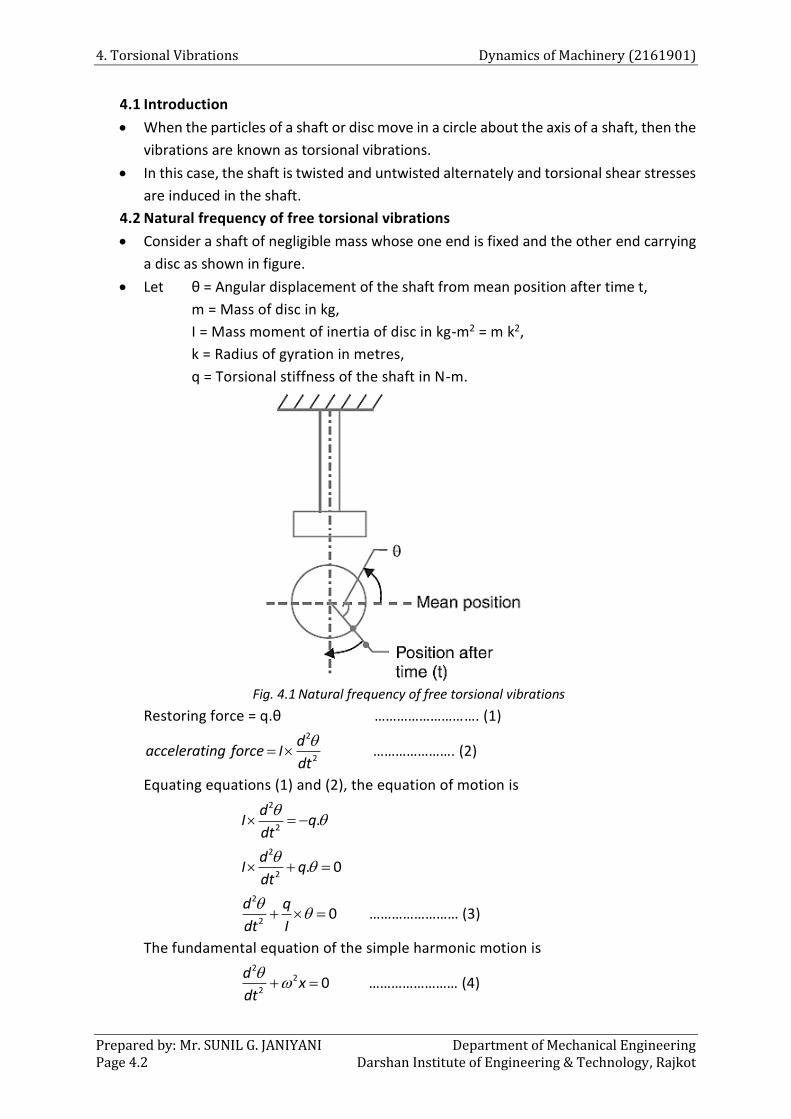
4. Torsional Vibrations Dynamics of Machinery (2161901)
Prepared by: Mr. SUNIL G. JANIYANI Department of Mechanical Engineering Page 4.2 Darshan Institute of Engineering & Technology, Rajkot
4.1 Introduction
When the particles of a shaft or disc move in a circle about the axis of a shaft, then the
vibrations are known as torsional vibrations.
In this case, the shaft is twisted and untwisted alternately and torsional shear stresses
are induced in the shaft.
4.2 Natural frequency of free torsional vibrations
Consider a shaft of negligible mass whose one end is fixed and the other end carrying
a disc as shown in figure.
Let θ = Angular displacement of the shaft from mean position after time t,
m = Mass of disc in kg,
I = Mass moment of inertia of disc in kg-m2 = m k2,
k = Radius of gyration in metres,
q = Torsional stiffness of the shaft in N-m.
Fig. 4.1 Natural frequency of free torsional vibrations
Restoring force = q.θ ………………………. (1) 2
2
daccelerating force I
dt
…………………. (2)
Equating equations (1) and (2), the equation of motion is 2
2.
dI q
dt
2
2. 0
dI q
dt
2
20
d q
dt I
…………………… (3)
The fundamental equation of the simple harmonic motion is 2
2
20
dx
dt
…………………… (4)
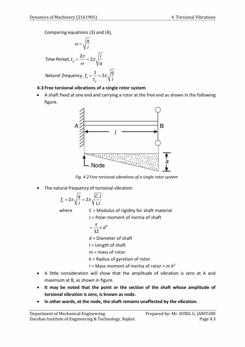
Dynamics of Machinery (2161901) 4. Torsional Vibrations
Department of Mechanical Engineering Prepared by: Mr. SUNIL G. JANIYANI Darshan Institute of Engineering & Technology, Rajkot Page 4.3
Comparing equations (3) and (4),
q
I
2, 2p
ITime Period t
q
1, 2n
p
qNatural frequency f
t I
4.3 Free torsional vibrations of a single rotor system
A shaft fixed at one end and carrying a rotor at the free end as shown in the following
figure.
Fig. 4.2 Free torsional vibrations of a single rotor system
The natural frequency of torsional vibration
.2 2
.n
q C Jf
I L I
where C = Modulus of rigidity for shaft material
J = Polar moment of inertia of shaft
4
32d
d = Diameter of shaft
l = Length of shaft
m = mass of rotor
k = Radius of gyration of rotor
I = Mass moment of inertia of rotor = m k2
A little consideration will show that the amplitude of vibration is zero at A and
maximum at B, as shown in figure.
It may be noted that the point or the section of the shaft whose amplitude of
torsional vibration is zero, is known as node.
In other words, at the node, the shaft remains unaffected by the vibration.
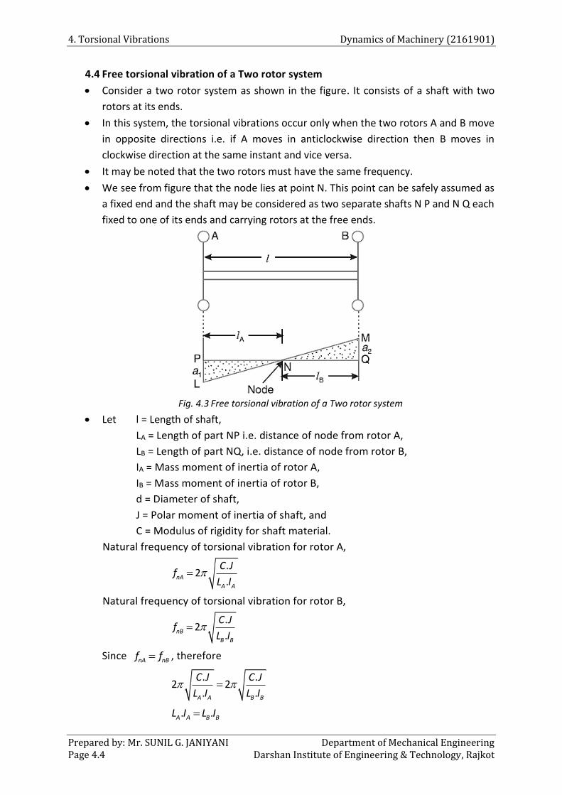
4. Torsional Vibrations Dynamics of Machinery (2161901)
Prepared by: Mr. SUNIL G. JANIYANI Department of Mechanical Engineering Page 4.4 Darshan Institute of Engineering & Technology, Rajkot
4.4 Free torsional vibration of a Two rotor system
Consider a two rotor system as shown in the figure. It consists of a shaft with two
rotors at its ends.
In this system, the torsional vibrations occur only when the two rotors A and B move
in opposite directions i.e. if A moves in anticlockwise direction then B moves in
clockwise direction at the same instant and vice versa.
It may be noted that the two rotors must have the same frequency.
We see from figure that the node lies at point N. This point can be safely assumed as
a fixed end and the shaft may be considered as two separate shafts N P and N Q each
fixed to one of its ends and carrying rotors at the free ends.
Fig. 4.3 Free torsional vibration of a Two rotor system
Let l = Length of shaft,
LA = Length of part NP i.e. distance of node from rotor A,
LB = Length of part NQ, i.e. distance of node from rotor B,
IA = Mass moment of inertia of rotor A,
IB = Mass moment of inertia of rotor B,
d = Diameter of shaft,
J = Polar moment of inertia of shaft, and
C = Modulus of rigidity for shaft material.
Natural frequency of torsional vibration for rotor A,
.2
.nA
A A
C Jf
L I
Natural frequency of torsional vibration for rotor B,
.2
.nB
B B
C Jf
L I
Since nA nBf f , therefore
. .2 2
. .A A B B
C J C J
L I L I
. .A A B BL I L I
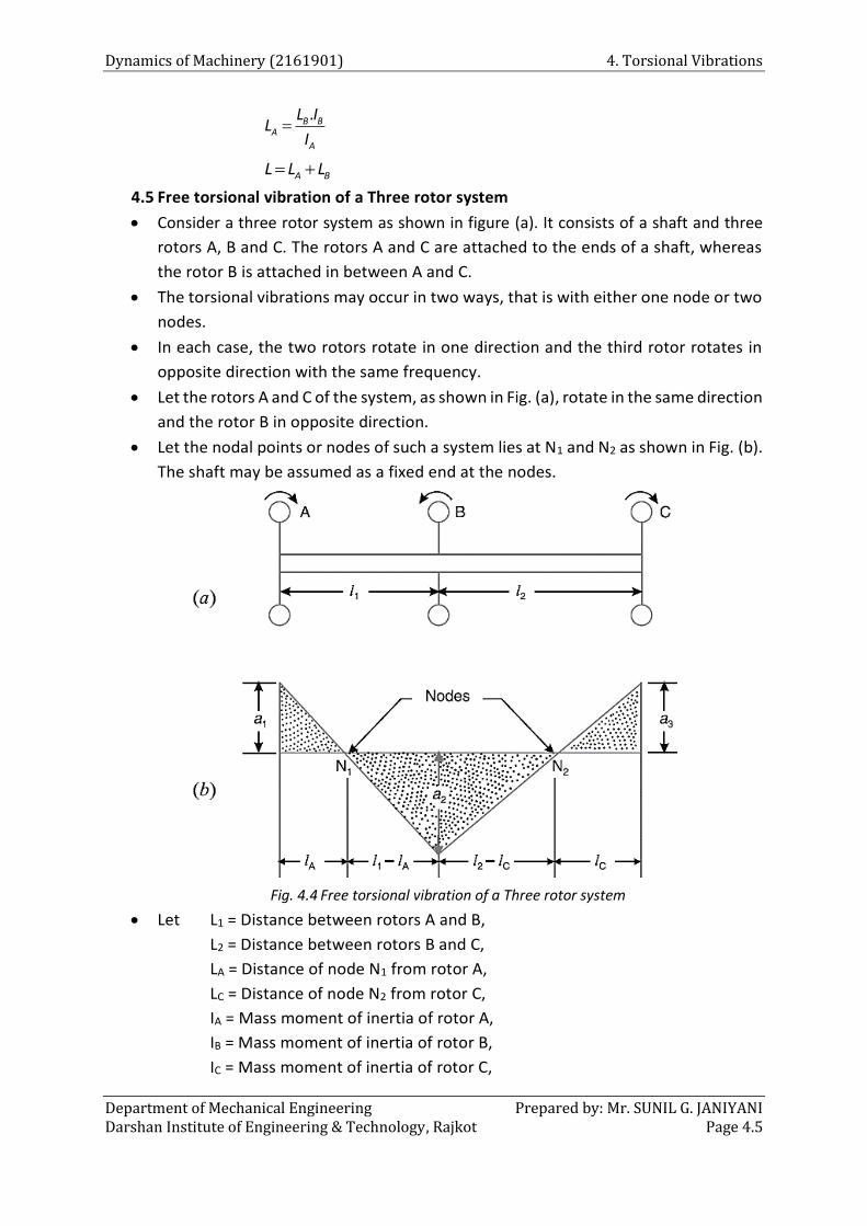
Dynamics of Machinery (2161901) 4. Torsional Vibrations
Department of Mechanical Engineering Prepared by: Mr. SUNIL G. JANIYANI Darshan Institute of Engineering & Technology, Rajkot Page 4.5
.B BA
A
L IL
I
A BL L L
4.5 Free torsional vibration of a Three rotor system
Consider a three rotor system as shown in figure (a). It consists of a shaft and three
rotors A, B and C. The rotors A and C are attached to the ends of a shaft, whereas
the rotor B is attached in between A and C.
The torsional vibrations may occur in two ways, that is with either one node or two
nodes.
In each case, the two rotors rotate in one direction and the third rotor rotates in
opposite direction with the same frequency.
Let the rotors A and C of the system, as shown in Fig. (a), rotate in the same direction
and the rotor B in opposite direction.
Let the nodal points or nodes of such a system lies at N1 and N2 as shown in Fig. (b).
The shaft may be assumed as a fixed end at the nodes.
Fig. 4.4 Free torsional vibration of a Three rotor system
Let L1 = Distance between rotors A and B,
L2 = Distance between rotors B and C,
LA = Distance of node N1 from rotor A,
LC = Distance of node N2 from rotor C,
IA = Mass moment of inertia of rotor A,
IB = Mass moment of inertia of rotor B,
IC = Mass moment of inertia of rotor C,
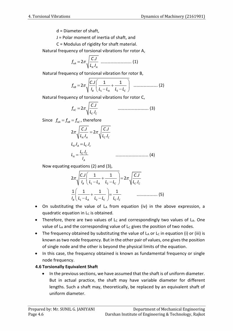
4. Torsional Vibrations Dynamics of Machinery (2161901)
Prepared by: Mr. SUNIL G. JANIYANI Department of Mechanical Engineering Page 4.6 Darshan Institute of Engineering & Technology, Rajkot
d = Diameter of shaft,
J = Polar moment of inertia of shaft, and
C = Modulus of rigidity for shaft material.
Natural frequency of torsional vibrations for rotor A,
.2
.nA
A A
C Jf
L I ………………………. (1)
Natural frequency of torsional vibration for rotor B,
1 2
. 1 12nB
B A C
C Jf
I L L L L
…………………. (2)
Natural frequency of torsional vibrations for rotor C,
.2
.nC
C C
C Jf
L I ………………………. (3)
Since nA nB nCf f f , therefore
. .2 2
. .A A C C
C J C J
L I L I
. .A A C cL I L I
.C CA
A
L IL
I ………………………… (4)
Now equating equations (2) and (3),
1 2
. 1 1 .2 2
.B A C C C
C J C J
I L L L L L I
1 2
1 1 1 1
.B A C C CI L L L L L I
………………. (5)
On substituting the value of LA from equation (iv) in the above expression, a
quadratic equation in LC is obtained.
Therefore, there are two values of LC and correspondingly two values of LA. One
value of LA and the corresponding value of LC gives the position of two nodes.
The frequency obtained by substituting the value of LA or LC in equation (i) or (iii) is
known as two node frequency. But in the other pair of values, one gives the position
of single node and the other is beyond the physical limits of the equation.
In this case, the frequency obtained is known as fundamental frequency or single
node frequency.
4.6 Torsionally Equivalent Shaft
In the previous sections, we have assumed that the shaft is of uniform diameter.
But in actual practice, the shaft may have variable diameter for different
lengths. Such a shaft may, theoretically, be replaced by an equivalent shaft of
uniform diameter.
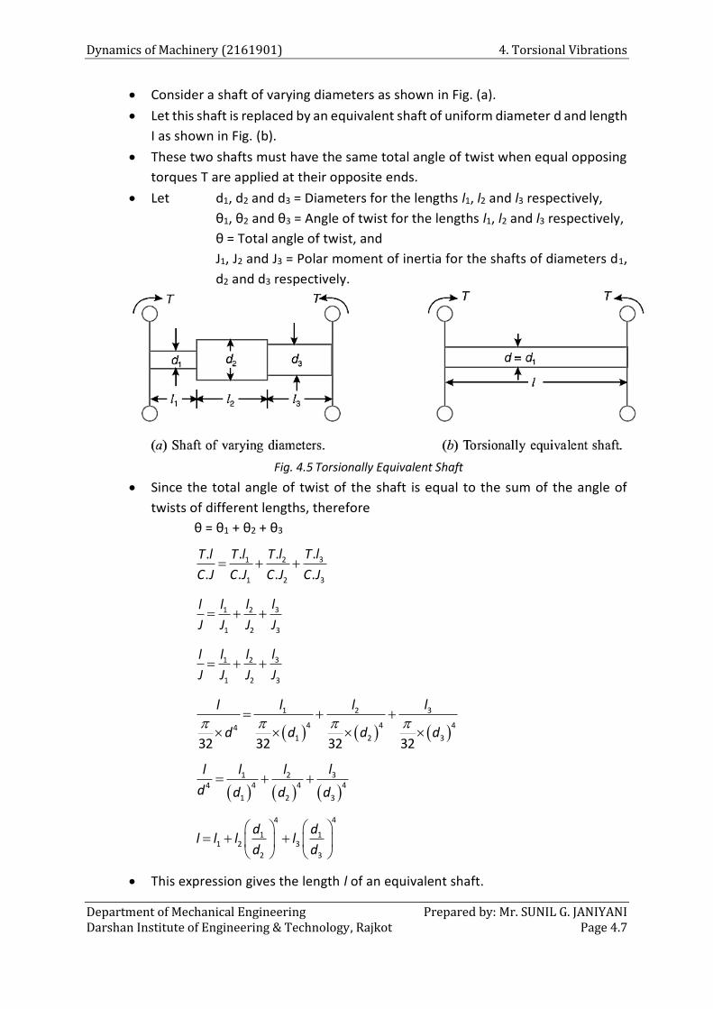
Dynamics of Machinery (2161901) 4. Torsional Vibrations
Department of Mechanical Engineering Prepared by: Mr. SUNIL G. JANIYANI Darshan Institute of Engineering & Technology, Rajkot Page 4.7
Consider a shaft of varying diameters as shown in Fig. (a).
Let this shaft is replaced by an equivalent shaft of uniform diameter d and length
I as shown in Fig. (b).
These two shafts must have the same total angle of twist when equal opposing
torques T are applied at their opposite ends.
Let d1, d2 and d3 = Diameters for the lengths l1, l2 and l3 respectively,
θ1, θ2 and θ3 = Angle of twist for the lengths l1, l2 and l3 respectively,
θ = Total angle of twist, and
J1, J2 and J3 = Polar moment of inertia for the shafts of diameters d1,
d2 and d3 respectively.
Fig. 4.5 Torsionally Equivalent Shaft
Since the total angle of twist of the shaft is equal to the sum of the angle of
twists of different lengths, therefore
θ = θ1 + θ2 + θ3
31 2
1 2 3
.. ..
. . . .
T lT l T lT l
C J C J C J C J
31 2
1 2 3
ll ll
J J J J
31 2
1 2 3
ll ll
J J J J
31 2
4 4 441 2 3
32 32 32 32
ll ll
d d d d
31 2
4 4 44
1 2 3
ll ll
d d d d
44
1 11 2 3
2 3
d dl l l l
d d
This expression gives the length l of an equivalent shaft.
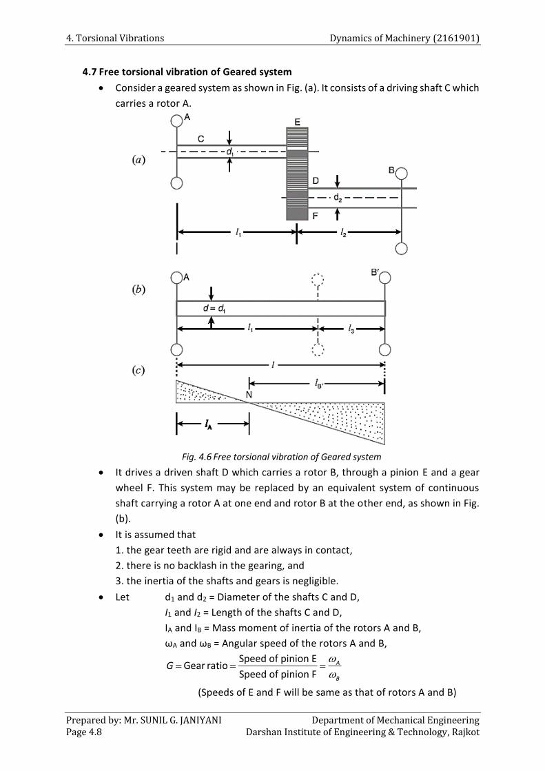
4. Torsional Vibrations Dynamics of Machinery (2161901)
Prepared by: Mr. SUNIL G. JANIYANI Department of Mechanical Engineering Page 4.8 Darshan Institute of Engineering & Technology, Rajkot
4.7 Free torsional vibration of Geared system
Consider a geared system as shown in Fig. (a). It consists of a driving shaft C which
carries a rotor A.
Fig. 4.6 Free torsional vibration of Geared system
It drives a driven shaft D which carries a rotor B, through a pinion E and a gear
wheel F. This system may be replaced by an equivalent system of continuous
shaft carrying a rotor A at one end and rotor B at the other end, as shown in Fig.
(b).
It is assumed that
1. the gear teeth are rigid and are always in contact,
2. there is no backlash in the gearing, and
3. the inertia of the shafts and gears is negligible.
Let d1 and d2 = Diameter of the shafts C and D,
I1 and I2 = Length of the shafts C and D,
IA and IB = Mass moment of inertia of the rotors A and B,
ωA and ωB = Angular speed of the rotors A and B,
Speed of pinion EGear ratio
Speed of pinion FA
B
G
(Speeds of E and F will be same as that of rotors A and B)
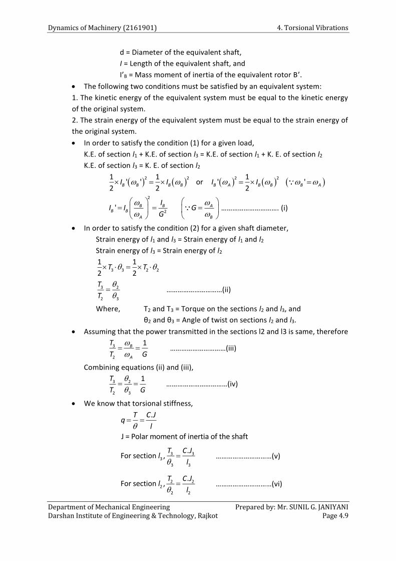
Dynamics of Machinery (2161901) 4. Torsional Vibrations
Department of Mechanical Engineering Prepared by: Mr. SUNIL G. JANIYANI Darshan Institute of Engineering & Technology, Rajkot Page 4.9
d = Diameter of the equivalent shaft,
I = Length of the equivalent shaft, and
I’B = Mass moment of inertia of the equivalent rotor B’.
The following two conditions must be satisfied by an equivalent system:
1. The kinetic energy of the equivalent system must be equal to the kinetic energy
of the original system.
2. The strain energy of the equivalent system must be equal to the strain energy of
the original system.
In order to satisfy the condition (1) for a given load,
K.E. of section l1 + K.E. of section l3 = K.E. of section l1 + K. E. of section l2
K.E. of section l3 = K. E. of section l2
2 2 2 21 1 1
' ' or ' '2 2 2
B B B B B A B B B AI I I I
2
2' B B A
B B
A B
II I G
G
…………………………. (i)
In order to satisfy the condition (2) for a given shaft diameter,
Strain energy of l1 and l3 = Strain energy of l1 and l2
Strain energy of l3 = Strain energy of l2
3 3 2 2
1 1
2 2T T
3 2
2 3
T
T
…………………………(ii)
Where, T2 and T3 = Torque on the sections l2 and l3, and
θ2 and θ3 = Angle of twist on sections l2 and l3.
Assuming that the power transmitted in the sections l2 and l3 is same, therefore
3
2
1B
A
T
T G
…………………………(iii)
Combining equations (ii) and (iii),
3 2
2 3
1T
T G
……………………………(iv)
We know that torsional stiffness,
.
J = Polar moment of inertia of the shaft
T C Jq
l
3 33
3 3
.For section ,
T C Jl
l …………………………(v)
2 22
2 2
.For section ,
T C Jl
l …………………………(vi)
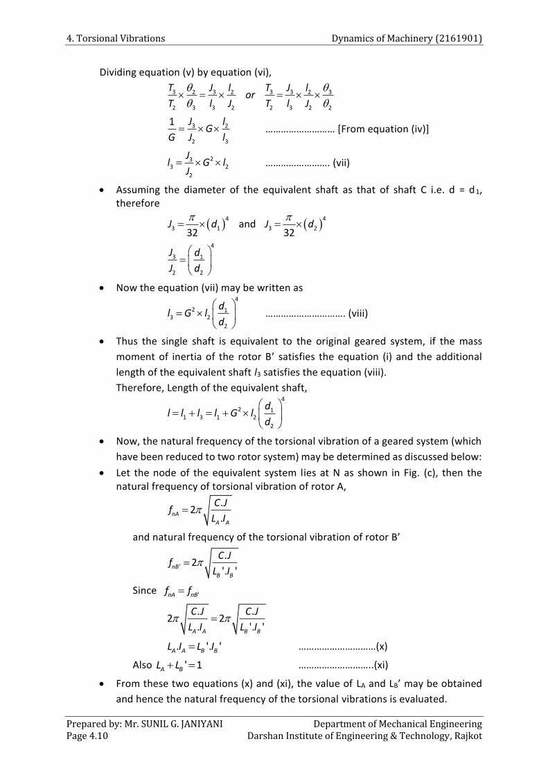
4. Torsional Vibrations Dynamics of Machinery (2161901)
Prepared by: Mr. SUNIL G. JANIYANI Department of Mechanical Engineering Page 4.10 Darshan Institute of Engineering & Technology, Rajkot
Dividing equation (v) by equation (vi),
3 3 3 3 32 2 2
2 3 3 2 2 3 2 2
T J T Jl lor
T l J T l J
3 2
2 3
1 J lG
G J l ……………………… [From equation (iv)]
233 2
2
Jl G l
J ……………………. (vii)
Assuming the diameter of the equivalent shaft as that of shaft C i.e. d = d1, therefore
4 4
3 1 3 2and32 32
J d J d
4
3 1
2 2
J d
J d
Now the equation (vii) may be written as 4
2 13 2
2
dl G l
d
…………………………. (viii)
Thus the single shaft is equivalent to the original geared system, if the mass
moment of inertia of the rotor B’ satisfies the equation (i) and the additional
length of the equivalent shaft l3 satisfies the equation (viii).
Therefore, Length of the equivalent shaft, 4
2 11 3 1 2
2
dl l l l G l
d
Now, the natural frequency of the torsional vibration of a geared system (which
have been reduced to two rotor system) may be determined as discussed below:
Let the node of the equivalent system lies at N as shown in Fig. (c), then the natural frequency of torsional vibration of rotor A,
.2
.nA
A A
C Jf
L I
and natural frequency of the torsional vibration of rotor B’
'
.2
'. 'nB
B B
C Jf
L I
Since 'nA nBf f
. .2 2
. '. 'A A B B
C J C J
L I L I
. '. 'A A B BL I L I …………………………(x)
Also ' 1A BL L ………………………..(xi)
From these two equations (x) and (xi), the value of LA and LB’ may be obtained
and hence the natural frequency of the torsional vibrations is evaluated.
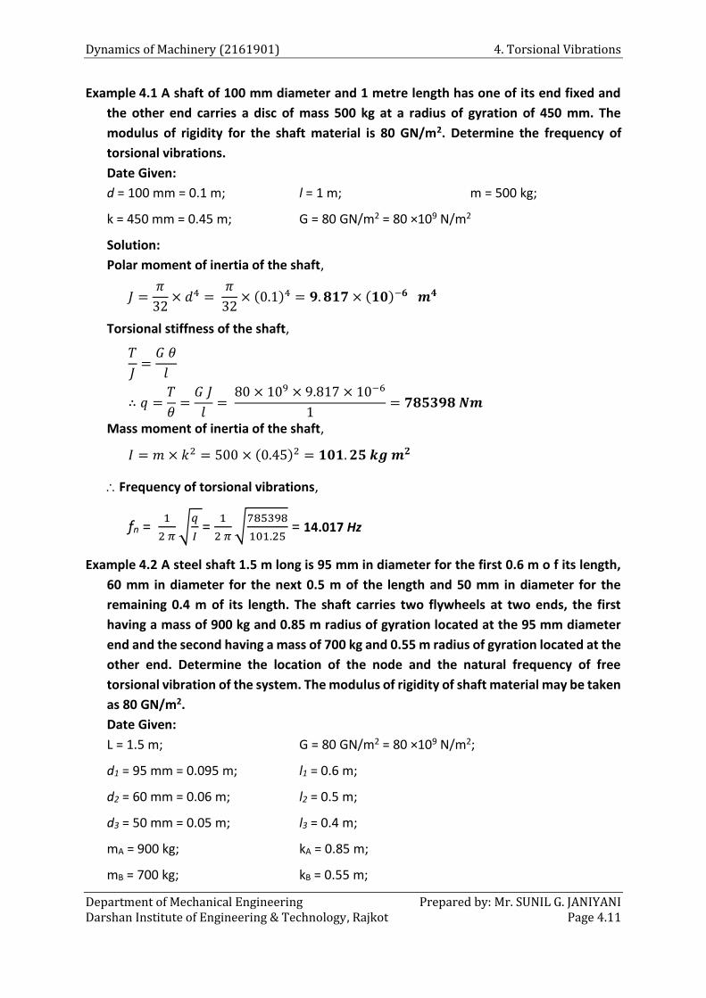
Dynamics of Machinery (2161901) 4. Torsional Vibrations
Department of Mechanical Engineering Prepared by: Mr. SUNIL G. JANIYANI Darshan Institute of Engineering & Technology, Rajkot Page 4.11
Example 4.1 A shaft of 100 mm diameter and 1 metre length has one of its end fixed and
the other end carries a disc of mass 500 kg at a radius of gyration of 450 mm. The
modulus of rigidity for the shaft material is 80 GN/m2. Determine the frequency of
torsional vibrations.
Date Given:
d = 100 mm = 0.1 m; l = 1 m; m = 500 kg;
k = 450 mm = 0.45 m; G = 80 GN/m2 = 80 ×109 N/m2
Solution:
Polar moment of inertia of the shaft,
𝐽 =𝜋
32× 𝑑4 =
𝜋
32× (0.1)4 = 𝟗. 𝟖𝟏𝟕 × (𝟏𝟎)−𝟔 𝒎𝟒
Torsional stiffness of the shaft,
𝑇
𝐽=
𝐺 𝜃
𝑙
∴ 𝑞 =𝑇
𝜃=
𝐺 𝐽
𝑙=
80 × 109 × 9.817 × 10−6
1= 𝟕𝟖𝟓𝟑𝟗𝟖 𝑵𝒎
Mass moment of inertia of the shaft,
𝐼 = 𝑚 × 𝑘2 = 500 × (0.45)2 = 𝟏𝟎𝟏. 𝟐𝟓 𝒌𝒈 𝒎𝟐
Frequency of torsional vibrations,
fn = 1
2 𝜋√
𝑞
𝐼 =
1
2 𝜋√
785398
101.25 = 14.017 Hz
Example 4.2 A steel shaft 1.5 m long is 95 mm in diameter for the first 0.6 m o f its length,
60 mm in diameter for the next 0.5 m of the length and 50 mm in diameter for the
remaining 0.4 m of its length. The shaft carries two flywheels at two ends, the first
having a mass of 900 kg and 0.85 m radius of gyration located at the 95 mm diameter
end and the second having a mass of 700 kg and 0.55 m radius of gyration located at the
other end. Determine the location of the node and the natural frequency of free
torsional vibration of the system. The modulus of rigidity of shaft material may be taken
as 80 GN/m2.
Date Given:
L = 1.5 m; G = 80 GN/m2 = 80 ×109 N/m2;
d1 = 95 mm = 0.095 m; l1 = 0.6 m;
d2 = 60 mm = 0.06 m; l2 = 0.5 m;
d3 = 50 mm = 0.05 m; l3 = 0.4 m;
mA = 900 kg; kA = 0.85 m;
mB = 700 kg; kB = 0.55 m;
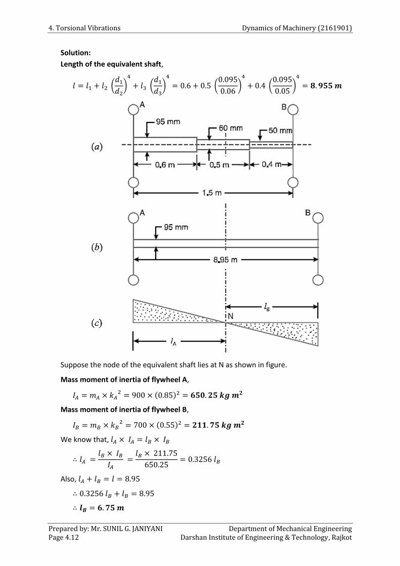
4. Torsional Vibrations Dynamics of Machinery (2161901)
Prepared by: Mr. SUNIL G. JANIYANI Department of Mechanical Engineering Page 4.12 Darshan Institute of Engineering & Technology, Rajkot
Solution:
Length of the equivalent shaft,
𝑙 = 𝑙1 + 𝑙2 (𝑑1
𝑑2)
4
+ 𝑙3 (𝑑1
𝑑3)
4
= 0.6 + 0.5 (0.095
0.06)
4
+ 0.4 (0.095
0.05)
4
= 𝟖. 𝟗𝟓𝟓 𝒎
Suppose the node of the equivalent shaft lies at N as shown in figure.
Mass moment of inertia of flywheel A,
𝐼𝐴 = 𝑚𝐴 × 𝑘𝐴2 = 900 × (0.85)2 = 𝟔𝟓𝟎. 𝟐𝟓 𝒌𝒈 𝒎𝟐
Mass moment of inertia of flywheel B,
𝐼𝐵 = 𝑚𝐵 × 𝑘𝐵2 = 700 × (0.55)2 = 𝟐𝟏𝟏. 𝟕𝟓 𝒌𝒈 𝒎𝟐
We know that, 𝑙𝐴 × 𝐼𝐴 = 𝑙𝐵 × 𝐼𝐵
∴ 𝑙𝐴 =𝑙𝐵 × 𝐼𝐵
𝐼𝐴 =
𝑙𝐵 × 211.75
650.25= 0.3256 𝑙𝐵
Also, 𝑙𝐴 + 𝑙𝐵 = 𝑙 = 8.95
∴ 0.3256 𝑙𝐵 + 𝑙𝐵 = 8.95
∴ 𝒍𝑩 = 𝟔. 𝟕𝟓 𝒎
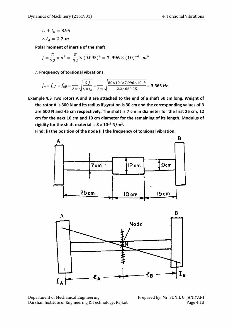
Dynamics of Machinery (2161901) 4. Torsional Vibrations
Department of Mechanical Engineering Prepared by: Mr. SUNIL G. JANIYANI Darshan Institute of Engineering & Technology, Rajkot Page 4.13
𝑙𝐴 + 𝑙𝐵 = 8.95
∴ 𝒍𝑨 = 𝟐. 𝟐 𝒎
Polar moment of inertia of the shaft,
𝐽 =𝜋
32× 𝑑4 =
𝜋
32× (0.095)4 = 𝟕. 𝟗𝟗𝟔 × (𝟏𝟎)−𝟔 𝒎𝟒
Frequency of torsional vibrations,
fn = fnA = fnB = 1
2 𝜋√
𝐺 𝐽
𝑙𝐴× 𝐼𝐴
= 1
2 𝜋√
80×109×7.996×10−6
2.2×650.25 = 3.365 Hz
Example 4.3 Two rotors A and B are attached to the end of a shaft 50 cm long. Weight of
the rotor A is 300 N and its radius if gyration is 30 cm and the corresponding values of B
are 500 N and 45 cm respectively. The shaft is 7 cm in diameter for the first 25 cm, 12
cm for the next 10 cm and 10 cm diameter for the remaining of its length. Modulus of
rigidity for the shaft material is 8 × 10¹¹ N/m2.
Find: (i) the position of the node (ii) the frequency of torsional vibration.
4. Torsional Vibrations Dynamics of Machinery (2161901)
Prepared by: Mr. SUNIL G. JANIYANI Department of Mechanical Engineering Page 4.14 Darshan Institute of Engineering & Technology, Rajkot
Date Given:
L = 50 cm = 0.5 m; G = 8 ×10¹¹ N/m2;
d1 = 7 cm = 0.07 m; l1 = 25 cm = 0.25 m;
d2 = 12 cm = 0.12 m; l2 = 10 cm = 0.1 m;
d3 = 10 cm = 0.1 m; l3 = 15 cm = 0.15 m;
WA = 300 N; kA = 30 cm = 0.3 m;
WB = 500 N; kB = 45 cm = 0.45 m;
Solution:
Length of the equivalent shaft,
𝑙 = 𝑙1 + 𝑙2 (𝑑1
𝑑2)
4
+ 𝑙3 (𝑑1
𝑑3)
4
= 0.25 + 0.1 (0.07
0.12)
4
+ 0.15 (0.07
0.1)
4
= 𝟎. 𝟐𝟗𝟕𝟓 𝒎
Suppose the node of the equivalent shaft lies at N as shown in figure.
Mass moment of inertia of flywheel A,
𝐼𝐴 = 𝑚𝐴 × 𝑘𝐴2 =
𝑊𝐴
𝑔× 𝑘𝐴
2 = 300
9.81× (0.3)2 = 𝟐. 𝟕𝟓𝟐𝟑 𝒌𝒈 𝒎𝟐
Mass moment of inertia of flywheel B,
𝐼𝐵 = 𝑚𝐵 × 𝑘𝐵2 =
𝑊𝐵
𝑔× 𝑘𝐵
2 = 500
9.81× (0.45)2 = 𝟏𝟎. 𝟑𝟐𝟏𝟏 𝒌𝒈 𝒎𝟐
We know that, 𝑙𝐴 × 𝐼𝐴 = 𝑙𝐵 × 𝐼𝐵
∴ 𝑙𝐴 =𝑙𝐵 × 𝐼𝐵
𝐼𝐴 =
𝑙𝐵 × 10.3211
2.7523= 3.75 𝑙𝐵
Also, 𝑙𝐴 + 𝑙𝐵 = 𝑙 = 0.5
∴ 3.75 𝑙𝐵 + 𝑙𝐵 = 0.2975
∴ 𝒍𝑩 = 𝟎. 𝟎𝟔𝟐𝟔 𝒎
𝑙𝐴 + 𝑙𝐵 = 0.2975
∴ 𝒍𝑨 = 𝟎. 𝟐𝟑𝟒𝟖 𝒎
Polar moment of inertia of the shaft,
𝐽 =𝜋
32× 𝑑4 =
𝜋
32× (0.07)4 = 𝟐. 𝟑𝟓𝟕 × (𝟏𝟎)−𝟔 𝒎𝟒
Frequency of torsional vibrations,
fn = fnA = fnB = 1
2 𝜋√
𝐺 𝐽
𝑙𝐴× 𝐼𝐴
= 1
2 𝜋√
8×1011×2.357×10−6
0.2348×2.7523 = 271.87 Hz
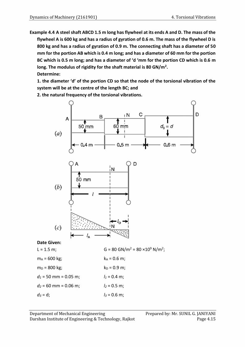
Dynamics of Machinery (2161901) 4. Torsional Vibrations
Department of Mechanical Engineering Prepared by: Mr. SUNIL G. JANIYANI Darshan Institute of Engineering & Technology, Rajkot Page 4.15
Example 4.4 A steel shaft ABCD 1.5 m long has flywheel at its ends A and D. The mass of the
flywheel A is 600 kg and has a radius of gyration of 0.6 m. The mass of the flywheel D is
800 kg and has a radius of gyration of 0.9 m. The connecting shaft has a diameter of 50
mm for the portion AB which is 0.4 m long; and has a diameter of 60 mm for the portion
BC which is 0.5 m long; and has a diameter of ‘d ‘mm for the portion CD which is 0.6 m
long. The modulus of rigidity for the shaft material is 80 GN/m2.
Determine:
1. the diameter ‘d’ of the portion CD so that the node of the torsional vibration of the
system will be at the centre of the length BC; and
2. the natural frequency of the torsional vibrations.
Date Given:
L = 1.5 m; G = 80 GN/m2 = 80 ×109 N/m2;
mA = 600 kg; kA = 0.6 m;
mD = 800 kg; kD = 0.9 m;
d1 = 50 mm = 0.05 m; l1 = 0.4 m;
d2 = 60 mm = 0.06 m; l2 = 0.5 m;
d3 = d; l3 = 0.6 m;
4. Torsional Vibrations Dynamics of Machinery (2161901)
Prepared by: Mr. SUNIL G. JANIYANI Department of Mechanical Engineering Page 4.16 Darshan Institute of Engineering & Technology, Rajkot
Solution:
Length of the equivalent shaft,
𝑙 = 𝑙1 + 𝑙2 (𝑑1
𝑑2)
4
+ 𝑙3 (𝑑1
𝑑3)
4
= 0.4 + 0.5 (0.05
0.06)
4
+ 0.6 (0.05
𝑑)
4
= 0.641 +3.75 × 10⁻⁶
𝑑4⋯ ⋯ ⋯ ⋯ ⋯ (𝑖)
Suppose the node of the equivalent shaft lies at N as shown in figure.
Mass moment of inertia of flywheel A,
𝐼𝐴 = 𝑚𝐴 × 𝑘𝐴2 = 600 × (0.6)2 = 𝟐𝟏𝟔 𝒌𝒈 𝒎𝟐
Mass moment of inertia of flywheel D,
𝐼𝐷 = 𝑚𝐷 × 𝑘𝐷2 = 800 × (0.9)2 = 𝟔𝟒𝟖 𝒌𝒈 𝒎𝟐
We know that, 𝑙𝐴 × 𝐼𝐴 = 𝑙𝐷 × 𝐼𝐷
∴ 𝑙𝐴 =𝑙𝐷 × 𝐼𝐷
𝐼𝐴 =
𝑙𝐷 × 648
216= 3 𝑙𝐷
Since the node lies at the centre of the length BC in original system, therefore its
equivalent length from rotor A,
𝑙𝐴 = 𝑙1 +𝑙2
2 (
𝑑1
𝑑2)
4
= 0.4 +0.5
2 (
0.05
0.06)
4
= 𝟎. 𝟓𝟐 𝒎
𝑙𝐴 = 3 𝑙𝐷
∴ 𝑙𝐷 = 𝑙𝐴
3 =
0.52
3= 𝟎. 𝟏𝟕𝟑𝟓 𝒎
Also, 𝑙𝐴 + 𝑙𝐷 = 𝑙 = 0.641 +3.75×10⁻⁶
𝑑4 (From equation (i))
∴ 0.52 + 0.1735 = 0.641 +3.75 × 10⁻⁶
𝑑4
∴ 0.05252 =3.75 × 10⁻⁶
𝑑4
∴ 𝑑4 =3.75 × 10⁻⁶
0.05252
∴ 𝒅 = 𝟎. 𝟎𝟗𝟏𝟗𝟐 𝒎 = 𝟗𝟏. 𝟗𝟐 𝒎𝒎
Polar moment of inertia of the shaft,
𝐽 =𝜋
32× 𝑑1
4 = 𝜋
32× (0.05)4 = 𝟎. 𝟔𝟏𝟑𝟔 × (𝟏𝟎)−𝟔 𝒎𝟒
Frequency of torsional vibrations,
fn = fnA = fnB = 1
2 𝜋√
𝐺 𝐽
𝑙𝐴× 𝐼𝐴
= 1
2 𝜋√
80×109×0.6136×10−6
0.52×216 = 3.327 Hz
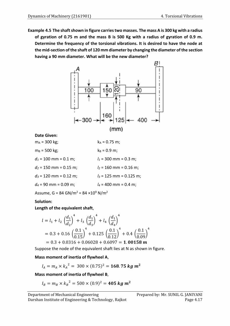
Dynamics of Machinery (2161901) 4. Torsional Vibrations
Department of Mechanical Engineering Prepared by: Mr. SUNIL G. JANIYANI Darshan Institute of Engineering & Technology, Rajkot Page 4.17
Example 4.5 The shaft shown in figure carries two masses. The mass A is 300 kg with a radius
of gyration of 0.75 m and the mass B is 500 Kg with a radius of gyration of 0.9 m.
Determine the frequency of the torsional vibrations. It is desired to have the node at
the mid-section of the shaft of 120 mm diameter by changing the diameter of the section
having a 90 mm diameter. What will be the new diameter?
Date Given:
mA = 300 kg; kA = 0.75 m;
mB = 500 kg; kB = 0.9 m;
d1 = 100 mm = 0.1 m; l1 = 300 mm = 0.3 m;
d2 = 150 mm = 0.15 m; l2 = 160 mm = 0.16 m;
d3 = 120 mm = 0.12 m; l3 = 125 mm = 0.125 m;
d4 = 90 mm = 0.09 m; l4 = 400 mm = 0.4 m;
Assume, G = 84 GN/m2 = 84 ×109 N/m2
Solution:
Length of the equivalent shaft,
𝑙 = 𝑙1 + 𝑙2 (𝑑1
𝑑2)
4
+ 𝑙3 (𝑑1
𝑑3)
4
+ 𝑙4 (𝑑1
𝑑4)
4
= 0.3 + 0.16 (0.1
0.15)
4
+ 0.125 (0.1
0.12)
4
+ 0.4 (0.1
0.09)
4
= 0.3 + 0.0316 + 0.06028 + 0.6097 = 𝟏. 𝟎𝟎𝟏𝟓𝟖 𝒎
Suppose the node of the equivalent shaft lies at N as shown in figure.
Mass moment of inertia of flywheel A,
𝐼𝐴 = 𝑚𝐴 × 𝑘𝐴2 = 300 × (0.75)2 = 𝟏𝟔𝟖. 𝟕𝟓 𝒌𝒈 𝒎𝟐
Mass moment of inertia of flywheel B,
𝐼𝐵 = 𝑚𝐵 × 𝑘𝐵2 = 500 × (0.9)2 = 𝟒𝟎𝟓 𝒌𝒈 𝒎𝟐
4. Torsional Vibrations Dynamics of Machinery (2161901)
Prepared by: Mr. SUNIL G. JANIYANI Department of Mechanical Engineering Page 4.18 Darshan Institute of Engineering & Technology, Rajkot
We know that, 𝑙𝐴 × 𝐼𝐴 = 𝑙𝐵 × 𝐼𝐵
∴ 𝑙𝐴 =𝑙𝐵 × 𝐼𝐵
𝐼𝐴 =
𝑙𝐵 × 405
168.75= 2.4 𝑙𝐵
Also, 𝑙𝐴 + 𝑙𝐵 = 𝑙 = 1.00158
∴ 2.4 𝑙𝐵 + 𝑙𝐵 = 1.00158
∴ 𝒍𝑩 = 𝟎. 𝟐𝟗𝟒𝟓 𝒎
𝑙𝐴 = 2.4 𝑙𝐵 = 2.4(0.2945) = 𝟎. 𝟕𝟎𝟕 𝒎
Polar moment of inertia of the shaft,
𝐽 =𝜋
32× 𝑑1
4 = 𝜋
32× (0.1)4 = 𝟗. 𝟖𝟏𝟕𝟓 × (𝟏𝟎)−𝟔 𝒎𝟒
Frequency of torsional vibrations,
fn = fnA = fnB = 1
2 𝜋√
𝐺 𝐽
𝑙𝐴× 𝐼𝐴
= 1
2 𝜋√
84×109×9.8175×10−6
0.707×168.75 = 13.23 Hz
It is desired to have the node at the mid-section of the shaft of 120 mm diameter by
changing the diameter of the section having a 90 mm diameter,
∴ 𝑙𝐴′ = 𝑙1 + 𝑙2 (
𝑑1
𝑑2)
4
+𝑙3
2 (
𝑑1
𝑑3)
4
= 0.3 + 0.16 (0.1
0.15)
4
+0.125
2(
0.1
0.12)
4
= 0.3 + 0.0316 + 0.03014 = 𝟎. 𝟑𝟔𝟏𝟕 𝒎
Also, 𝑙𝐴′ × 𝐼𝐴 = 𝑙𝐵
′ × 𝐼𝐵
∴ 0.3617 × 168.75 = 𝑙𝐵′ × 405
∴ 𝒍𝑩′ = 𝟎. 𝟏𝟓𝟎𝟕 𝒎
Also,
𝑙𝐵′ =
𝑙3
2 (
𝑑1
𝑑3)
4
+ 𝑙4 (𝑑1
𝑑)
4
∴ 0.1507 =0.125
2 (
0.1
0.12)
4
+ 0.4 (0.1
𝑑)
4
∴ 0.1507 = 0.03 + 0.4 (0.1
𝑑)
4
∴ 0.1206 = 0.4 (0.1
𝑑)
4
∴ 0.3014 = (0.1
𝑑)
4
∴ 0.7409 =0.1
𝑑
∴ 𝒅 = 𝟎. 𝟏𝟑𝟓 𝒎 = 𝟏𝟑𝟓 𝒎𝒎