Balance of Payment Dynamic in Indonesia and

Economics and Finance in IndonesiaVol. 63 No. 1, June 2017 : 53–80

p-ISSN 0126-155X; e-ISSN 2442-9260 53

Balance of Payment Dynamic in Indonesia andthe Structure of Economy I

Telisa Faliantya,∗

aDepartment of Economics, Faculty of Economics and Business Universitas Indonesia

Abstract

This paper will assess in aggregate and detail the trend of BOP and its component in Indonesia. Stationaritytest will be employed to each component of Indonesian BOP to assess the persistency. This study willcalculate the balance of payment constrained growth (BOPC) using Kalman Filter technique (state spacemodel). The BOP, secondary income, and financial account are found to be stationer which means thatthe data are mean reverting. On the other hand, current account balance, trade balance, service balance,primary income, and capital account balance are unit root. This paper found the evidence of the importanceof commodity price to Indonesian current account and export. Indonesian dependency on commodity-basedexport need to be restructured. Indonesia should also consider the side effect of FDI as a source of financingfor current account deficit, without ignoring the positive effect of FDI and the volatility of portfolio investment.The persistency of primary income deficit should also become Indonesian future policy agenda.Keywords: balance of payment; economic structure; macroeconomics; Indonesian economy

AbstrakMakalah ini menganalisis secara makro dan rinci tentang neraca pembayaran Indonesia dan komponen-komponennya. Uji stasioner dilakukan pada tiap komponen neraca pembayaran Indonesia untukmendapatkan ketepatan. Makalah ini mengadopsi perhitungan BOPC (balance of payment constrainedgrowth) dengan teknis Kalman Filter. Hasilnya neraca pembayaran, pendapatan sekunder dan neraca keuan-gan bersifat stasioner sementara neraca transaksi berjalan, neraca jasa, neraca perdagangan, pendapatanprimer dan neraca modal bersifat tidak stasioner. Makalah ini membuktikan bahwa harga komoditi primersangat penting bagi neraca transaksi berjalan dan ekspor nasional. Ketergantungan Indonesia pada komoditiprimer sangat besar sehingga harus dikurangi. Caranya adalah dengan meningkatkan peran investasi asingjangka panjang dan jangka pendek. Upaya mengatasi defisit neraca pendapatan primer harus menjadiagenda jangka panjang utama.Kata kunci: neraca pembayaran; struktur ekonomi; makroekonomi; ekonomi Indonesian

JEL classifications: F32; F41; E60

1. Introduction

IMF (2016) noted that the sum of net non-reservecapital inflows and the current account balance wasequal to the changes in foreign reserves under thebalance of payments identity. It also stated that

IAcknowledgment: Special thanks to Sri Andaiyani for herhelpful assistance in data collecting and processing.

∗Corresponding Author: MPKP FEB UI, Jalan Salemba Raya4 Kampus UI Salemba 10430. E-mail: [email protected].

the three components of the identity are jointly de-termined. As an illustration, during the years lead-ing up to the global financial crisis (GFC), therewere many commodity-exporting emerging mar-ket economies (including Indonesia) that receivedstrong capital inflows during the rising investmentopportunities and accumulated reserves, in addi-tion to strong terms-of-trade gains offsetting the im-pact of rapid import growth on the current account.However, from 2011 onward, the process started to

Economics and Finance in Indonesia Vol. 63 No. 1, June 2017

[email protected]

FALIANTY, T./BALANCE OF PAYMENT DYNAMIC...54

reverse as the commodity prices declining and thegrowth prospects becoming more subdued. The ex-planation of this general pattern by IMF also appliedin Indonesia’s case.

The ups and downs of commodity prices have beenaffecting the dynamics of BoPs in several emergingmarkets, including Indonesia. Besides the commod-ity prices, the quantitative-easing (QE) shocks alsohave some effect on the BoP dynamics. There isa strong relationship between the peak periods oflarge capital inflows (which mostly consists of port-folio inflows) in Indonesia and the United States’QE policy. The declining trend of capital inflows inIndonesia after 2013 has been largely influencedby the exit from the Fed’s accommodative monetarypolicy. Since the beginning of a gradual exit fromaccommodative monetary policy in the U.S., manycountries have been increasingly exposed to fluc-tuations in global uncertainty. Andaiyani & Falianty(2017) suggested that the increase in global uncer-tainty was one of the factors that induced fluctua-tions in the capital flow to Emerging Market Eco-nomics (EMEs).

The importance of understanding BoP dynamicsis related to the concept of Balance-of-Payments-Constrained (BOPC) Growth. This concept explainsthe mechanism of how BoP dynamics can influencethe dynamics of economic growth. BoP sustainabil-ity is considered to be a key factor in achievingsustainable growth. The previous studies related toBOPC growth concept are from Thrillwall (1979),Felipe, Mc Combie & Naqvi (2010), Felipe & Lan-zafame (2017).

To smooth the volatility in BoP dynamics, IMF (2016)emphasized the importance of mitigation policiesto anticipate global factors that could influenceBoP sustainability. Such policies are required tominimize each country’s vulnerabilities to globalrisk factors. These policies include prudent fiscalpolicies, proactive macro-prudential policies, flexi-

ble exchange-rate, and improved foreign exchangemanagement. In addition to these suggested poli-cies from IMF, we should also consider policies thatare related to the economic structure of the coun-try. The structure of a country may have a strongcorrelation with the BoP dynamics, especially thestructure of its international trade. In the case ofIndonesia as one of the exporting countries whichare highly dependent on primary commodities, thecommodity price upswings will greatly influence thetrade balance. Indonesia’s ongoing structural de-pendency on the export of primary commoditiesis classified as a structural factor that needs to beaddressed by policymakers. More structural fac-tors would be explored in this research. This papershall assess the trends of Indonesia’s BoP and itscomponents by the aggregates and details. Afteridentifying the patterns of BoP components, we canidentify the correlation between the patterns and thestructural distortions in the economy of Indonesia.

Figure 1: Indonesian Balance of Payment in MillionUSD, 2004Q1–2016Q4

Source: External Statistics, Economics and Finance Statistics,Central Bank of Indonesia

There are two objectives of this study. The first ob-jective is to identify the dynamics of BoP and BoPcomponents in Indonesia. The second one is toassess the relationship between the BoP dynamicsand the economic structure of Indonesia, as wellas its correlation to BOPC growth. UnderstandingBoP dynamics would be essential for measuring the


FALIANTY, T./BALANCE OF PAYMENT DYNAMIC... 55

external sustainability of Indonesia. External sus-tainability indicator is important as an early warningsystem indicator which can be used to formulatemacroeconomic policy to anticipate future situation.The relationship between BoP dynamics and In-donesia’s economic structure is important to em-phasize the importance of structural transformationin securing a sustainable external position for In-donesia as well as sustainable economic growth.

2. Literature Review

Internal balance is a term used to describe themacroeconomic goals of producing at potential out-put (at full employment) or also called normal pro-duction and of price stability (low inflation). Unsus-tainable use of resources (over employment) inwhich the demand for resources exceeds the avail-able supply tends to increase prices, meanwhile,an underemployment where the available supplyis not optimally used is inefficient and tends to de-crease prices. Both of which can hinder a countryfrom achieving internal balance by reducing theeconomy’s efficiency. As for external balance, it isachieved when an optimal level of the account bal-ance is attained. Optimal balance refers to the ex-ternal balance achieved when "a country’s currentaccount is neither so deeply in the deficit that thecountry may be unable to repay its foreign debts,nor it is so strongly in surplus that foreigners are putin that position" (Krugmman & Obstfeld 2003). Inother words, external balance can also be definedas the condition in which neither excessive currentaccount deficit nor excessive current account sur-plus is observed within an economy.

The basic theory of the balance of payment andcurrent account sustainability is needed to under-stand the framework of BoP dynamics and current

account sustainability.

(1)Y = C + I + G + X−M

where Y is Gross Domestic Product (GDP), C isaggregate consumption, I is aggregate investment,G is government expenditure, and X −M is tradebalance (exports-imports).

As we define A = C + I + G, then Equation (1) isreduced to:

(2)Y −A = X−M

Equation (2) shows that the difference between do-mestic production and domestic absorption alwaysequals to the current account of the balance ofpayment. In this case, Equation (2) assumed thatcurrent account is only composed of net exports.

The framework of intertemporal approach to the cur-rent account will be addressed next as a part of thisstudy. Standard open-economy identity provides agood starting point for constructing an intertempo-ral current account framework. Therefore, we willdenote net exports or trade balance as NX, theprimary income balance as PI, and the secondaryincome balance as SI, then we can define the cur-rent account (CA) balance for Indonesia for anyperiod t, as:

(3)CAINAt = NXINA

t + PIINAt + SIINA

t

The standard income expenditure identity is givenby Equation (2). Note that YINA

t refers to GDP inperiod t, CINA

t refers to the household consumptionin period t, IINA

t refers to the domestic investmentin period t, and GINA

t refers to the government pur-chases in period t:

(4)YINAt = CINA

t + IINAt + GINA

t + NXINAt

If we add the primary income balance and the sec-ondary income balance and subtract the net taxes



Figure 2: External Balance

(denoted by TINAt ; or also called taxes net of trans-

fers) from both sides of the income-expenditureidentity, we obtain:

YINAt + PIINA

t + SIINAt − TINA

t = (5)

CINAt + IINA

t + GINAt + NXINA

t + PIINAt +

SIINAt − TINA

t

By combining Equation (1) and (3), and rearrangingterms yield:

(6)(YINAt + PIINA

t + SIINAt − TINA

t − CINAt )

+ (TINAt −GINA

t ) = IINAt + CAINA

t

The left-hand side of the above equation reflectsthe sum of private saving (YINA

t + PIINAt + SIINA

t −TINA

t −CINAt ) and public saving (TINA

t −GINAt ), and

therefore Equation (4) can be simplified to obtainthe important open-economy identity (note: SINA

t

denotes the national saving and is equal to theprivate saving plus public saving):

SINAt = IINA

t +CAINAt → SINA

t −IINAt = CAINA

t (7)

Another crucial open-economy identity can be de-rived from the BoP accounting system. The follow-ing crucial flow identity (based on the double-entrybook-keeping approach used in BoP accountingsystem) holds for each period (t):

CAINAt + KAINA

t + FAINAt = 0 (8)

The identity states that the sum of the current ac-count, the capital account (KA) as well as a finan-

cial account (FA) should be equal to zero. If In-donesia ran a current account deficit (CAINA

t < 0

and SINAt − IINA

t < 0), then a financial account sur-plus (FA_t^INA>0) is unavoidable (given that thecapital account is typically quite small and can of-ten be ignored). In other words, Indonesia’s currentaccount deficit reflects the net new acquisition offoreign claims on the Indonesian. This study willmap the dynamics of the current account balancein Indonesia during the observation period.

According to Thirlwall (1979), countries can run cur-rent account deficits in the short run but persistentCA deficits cannot be sustained and will sooneror later lead to the adjustment process. A coun-try’s current account deficit can be worse whenthe domestic assets owned by foreign residentsare greater than assets owned by domestic resi-dents. Although a country cannot grow faster thanits balance of payments equilibrium growth rate fora very long period, unless the country can financean ever-growing deficit, there is little to stop a coun-try from growing slower and accumulating largesurpluses (Thirlwall 2011). According to his theory,BoP can act as a constraint on long-run growth, solong-run growth must be consistent with the BoPequilibrium. Felipe, McCombie & Naqvi (2010) ap-plied the framework of Balance of Payment Con-strained Growth (BoPC growth) for Pakistan. Theyfound that Pakistan’s maximum growth rate whichwas consistent with the equilibrium on the basicbalance was approximately 5% per annum. Thisfigure was below the specified target (GDP growthrate target of 7–8% per annum in the long term).



BoPC growth framework has indicated several im-portant implications for Pakistan development policy.The sources of constraints that impede the highergrowth of exports were found to be the export struc-ture and the low export complexity (and sophistica-tion performances). With low export complexity, realexchange rate depreciation would not lead to animprovement in the current account. In their study,they gave the recommendation for Pakistan to shiftits export structure from the traditional export areastowards more sophisticated manufactured goodswith a higher income elasticity of demand.

Freytag (2008) explored the BoP Dynamics in SouthAfrica. He linked the BoP dynamics with the institu-tions and the economic performance of a country.He identified the institutional and microeconomicperspectives of the current account. The institu-tional aspects that were covered in the study in-cluding the degree of economic freedom, propertyright, regulations on economic activities, bureau-cratic hurdles, governance, equal opportunity, andfairness. Besides BoP dynamics, Freytag (2008)also explained the interaction between the currentaccount and the capital account. He also discussedthe policy issues stemmed from the imbalances inBoP.

Asmarani & Falianty (2014) used stationary andAutoregressive Distributed Lag (ARDL) Approachto testing the current account deficit persistencyand sustainability. They found that Indonesia’s cur-rent account deficit was persistent for the period of2004Q1-2014Q1. They also found that trade andservice balance of Indonesia was in an unsustain-able condition. The unsustainable condition wasmore severe in the service sector. Lau et al. (2001)found that five East Asia countries’ BoPs weremean reverting, by using the data from 1976Q1–2001Q4. By using data from before and after globalfinancial crisis period (1960Q1–2010Q4), Clower &Ito (2012) examined a panel of 71 sample countries,where they found patterns of persistence in the cur-

rent account deficits. Indonesia was also includedin their country sample countries.

Calderon, Chong & Loayza (1999) provided theevidence of the empirical linkage between currentaccount deficits (as a ratio to GNDI) and a broadset of main economic variables proposed by theliterature. They found that a rise in domestic out-put growth would generate a larger current accountdeficit which indicated that the domestic growth ratehad a greater positive association with the domes-tic investment than the national saving. They alsofound that temporary shocks in terms of trade werelinked to higher current account deficits. Addition-ally, they also found that the higher growth rates inindustrialized economies or the larger internationalinterest rates led to a reduction in the current ac-count deficits in developing economies. Moreover,Chen (2011) examined the possibility of the currentaccount deficits of OECD countries to be character-ized by a unit root process with regime switching. Inthis study, the econometric methodology of regime-switching has allowed analysts to distinguish pe-riods which were associated with unsustainableoutcomes from those in which the intertemporal na-tional long-run budget constraint (LRBC) held. Hepointed out that LRBC was not very likely to holdfor Australia, the Czech Republic, Hungary, NewZealand, Portugal, Finland, and Spain. Based onhis observation in this study, he noted a red flag re-garding the current account deficits observed in thestudied period which might not be on a sustainablepath and might lead the countries to face a seriousrisk.

In his study, Kumar (2007) Kumar (2007) highlightedsome benefits of FDI to emerging economies. Heobserved that in general, the foreign firms’ participa-tion in domestic business encouraged the transferof advanced technologies to the host country aswell as fostered human capital development by pro-viding training for their employees. He also consid-ered FDI to be more stable compared to other types



of capital flows. Many developing countries wereobserved to pursue FDI for the purpose of exportpromotion and not for production for the domesticeconomy. Kumar also remarked on how FDI was animportant channel for delivery of services acrossborders. Additionally, he noted that FDI could fi-nance current account deficits through its effecton investment or offset other financial transactions,such as increases in reserves or capital outflows.On the other hand, the negative effects of FDI wereclearly highlighted by Jaffri et al. (2012). This studyhas contributed to the existing empirical literatureshowing negative impacts of FDI inflows in Pakistan.The study found that in the case of Pakistan, FDIinflows had worsened the current account balancein Pakistan both for long-run and short-run withinthe period of 1983–2011. He used AutoregressiveDistributed Lag (ARDL) in his study. By using ARDLapproach of cointegration, the study found evidenceregarding how FDI inflows had worsened, specif-ically, the income account of the current accountbalance in Pakistan.

Felipe, Mc.Kombie & Naqvi (2010) discussed theapplication of Thirlwall’s law wherein the long run,no country could grow faster than the rate that wasconsistent with the balance of the current accountunless it could finance its ever-growing deficits. Thislaw implies that there is a growth rate which a coun-try cannot exceed for any length of time becausethe country will quickly run into balance of paymentdifficulties if the country ever crosses that certaingrowth rate. An increase in a country’s growth ratethrough domestic demand policy shall increase thegrowth in imports through the import demand func-tion, while the export growth is determined largelyby the growth of foreign markets, and remains unaf-fected.

In addition, Tsen (2014) investigated the impactof public sector budget on external balance inMalaysia. He focused on the impacts of consoli-dated public-sector finance and federal government

finance on the balance of trade, the balance of ser-vices, the balance of the current account and thebalance of payments in Malaysia. He found that abudget may reduce the imbalance of certain goodsand services, or one component of the balance ofpayments but not others due to different elastici-ties of goods and services. In short run, Malaysiangovernment might cut public spending to addressthe issues in the external balance. In the long-run,the focus should be on improving productivity andthe quality of products and services through tech-nological advancement to enhance the export com-petitiveness of Malaysia. Ajayi (2015) explored thedeterminants of the balance of payments in Nigeria.The result suggested that a larger exchange rateand a lesser monetary policy rate would raise thebalance of payments of the Nigerian economy.

3. Research Method and Data

Stationarity test would be applied to the BoP andits components in time series mode using unit rootAugmented Dickey-Fuller (ADF diagnostic) in orderto check the persistence of the balance of paymentcomponents. In addition, graphical representationwould be used to complement the analysis in orderto check the trends of the BoP and its components.The volatility of each component would be observedusing a coefficient variation. The failure to rejectthe unit root hypothesis could be interpreted as anevidence for the non-mean reverting behavior ofBoP components. The non-reverting behavior ofBoP components could become a warning sign forpolicymakers for either the persistence of deficitor persistence of surplus. From these two typesof trends, the most worrying concern is if there isa persistence of deficit. The initial hypothesis forthis part of the analysis is that there is a persistentbehavior of some components of BoP.

The following equation refers to Sastre (2015) to



explain the basic aspects of the current accountbehavior as one of the focus of this study.

The net trade is expressed as:

(9)XT − tc1T ∗MT

If BT is the amount of Net Foreign Assets held,assuming zero inflation and perfect mobility of cap-ital, the rates of return would be equal to the realinterest rate, therefore:

(10)XT − tc1T ∗MT + r ∗ BT−1 = ∆BT

where r ∗ BT−1 denotes payments on net foreigncapital holdings and ∆BT the net foreign asset po-sition, while XT, MT, and tcr denote exports, im-ports, and exchange rate respectively, all variablesexpressed in real prices. The left-hand side of theequation is the current account position and theright-hand side the capital account.

Considering (10), the long-run equilibrium of netforeign assets, when the initial net asset holding isgiven, must satisfy the following:

XT − tcIT ∗MT + r ∗ BT = BT+1 + tcrMT− BT

(11)BT =BT+1 + tcrMT −XT

1 + r

If tcrt, XT, and MT are constant, in the steady state,the net foreign asset holdings should satisfy

(12)XT − tcrMT + rBT = 0

Provided the transversality condition

∞∑S=1

BT + S

(1 + r)s=

∞∑S=1

XT+S − tcrMT+S

(1 + r)s= 0 (13)

The implication of these equations is that if thetrade deficit is larger than this, the current accountwould be unsustainable. In this point, we must dis-tinguish the current account sustainability from the

intertemporal approach to the current account. Ina dynamic general equilibrium model, the optimal-ity of consumption and savings decisions must beconsidered by combining the BoP with a simple in-tertemporal model of consumption (see Obstfeld &Rogoff 1996).

If we define domestic savings ST as ST = YT −IT −GT = CT + XT − tcrMT

BT = −XT − tcrMT

r

BT = −XT − tcrMT

r−∞∑S=1

XT+S − tcrMT+S

(1 + r)s

BT = −∞∑S=0

XT+S − tcrMT+S

(1 + r)s+1= −

∞∑S=0

ST+S − CT+S

(1 + r)s+1

(14)

If we derive consumption from the life cycle theory,we get:

CT =r

1 + rWT

Where wealth in the open economy is

WT =

∞∑S=0

ST+S

(1 + r)s+ BT

with the current account being

CAT = ST + rBT − CT (15)

Substituting in the current account would give:

(16)CAT = −∞∑S=0

ST − ST+S

(1 + r)s

=

−∞∑S=0

XT − tcrMT + CT − [XT+S − tcrMT+S + CT+S]

(1 + r)s

=

∞∑S=0

tcr[MT −MT+S]− [XT −XT+S] + CT+S − CT

(1 + r)s

Thus, in order to be sustainable, a current ac-count deficit must be offset by the present value



of changes in the current and future domestic sav-ings. This study would map the trend of currentaccount balance. The period of observation for thisstudy would be from 2004 to 2016, using quarterlydata. The data of BoP and its components are col-lected from the External Statistics of Central Bankof Indonesia. Meanwhile, the international macroe-conomic data as a supporting empirical evidenceare taken from World Bank database and Bank forInternational Settlement (BIS) database.

To complement this analysis, we also would runOLS regression model for testing the significanceof the commodity prices to Indonesia’s export whichis derived from the model in Senhadji & Montene-gro (1998) and Falianty (2015). Granger causalitytest also would be applied to see the correlation be-tween FDI and the current account variables basedon a study by Tobing (2014). The regression modelfor the export equation is stated by the followingequation:

(17)Log(EXPORT) = β0 + β1Log(GDPF)

+ β2Log(EXCH_RATE)

+ β3Log(COMPRICE)

EXPORT is the export rate of goods and services,EXCH_RATE is the nominal exchange rate, andGDPF is the world income, and COMPRICE is theinternational commodity price. Our initial hypothesisis that β3 have a positive and significant effect. Thishypothesis implies that the export rate of Indonesiadepends on the commodity prices. Furthermore, forthe Granger causality test, we predict that thereis a causality between FDI as a component of thefinancial account and the Current Account.

For the second part of the complementary analysis,we would run the state space model (Kalman Filteror linear quadratic estimation) and Hodrick-PrescottFilter to obtain the balance of payment equilibrium

growth rate.

(18)Xt =

�Pdt

Pft

ηZε

(19)Mt =

�Pdt

Pft

θYπ

where:

X : exports;M : imports;Y : domestic income;Z : world income;Pd : domestic price;Pf : foreign price;η : elasticity of export to price ratio;ε : elasticity of export to world income;θ : elasticity of import to price ratio;π : elasticity of import to domestic income.

In a growing economy, the long-run constraint ofthe BoP equilibrium requires the export rate andimport rate to grow at the same rate.

(20)η(Pdt − Pft) + εZt = θ(Pdt − Pft) + πgt

The assumption of purchasing power parity in thelong-run will result Pdt − Pft = 0, so we get

(21)εZt = πgt

Equation (18) can be rearranged as:

(22)gt =εZt

π

Because gt is the growth rate of GDP which equal-izes the rates of growth of exports and imports, gt

is the BOPC growth rate. Equation (19) identifiesthe factors that determine the BOPC growth ratenamely the elasticity of export to the world income(ε), the world income (z), and the elasticity of importto domestic income (π).



Following Felipe & Lanzafame (2017)), we wouldlike to find the time-varying BOPC growth rate for In-donesia. Previously, the BOPC growth rate typicallywas assumed to be constant, however, unless xt orzt is constant, the value of gt would change overtime with the change in the trends of export. Thebenefit of using time-varying estimator is the factthat we can account for changes in the structuralfeatures. In his study, Felipe used Kalman Filtermethod which also would be applied in this study.This study would use a state-space model withtime-varying parameters, consisting of the followingequations:

(23)mt = θtrpt + πtgt + ut

(24)θt = θt−1 + vt

(25)πt = πt−1 + vt

To eliminate the short-run fluctuations, HP Filter isused to obtaining the long run trend of the growthrate of export, import, and output. The parametersof θt and πt in Equation (24) are respectively thetime-varying price and income elasticity of imports.To estimate both parameters, Kalman Filter methodwould be used.

4. Results and Analysis

In the first stage Stationarity test is employed tothe main part component of BoP and BoP itselfin aggregate. The result of this stationarity test issummarized in Table 1. Non-stationary behavior isrepresented in the current account balance, tradebalance, services balance, primary income, andcapital account. On the other hand, the stationarybehavior is captured in aggregate BoP, secondaryincome, and financial account (even for financialaccount is weakly stationary).

The results of stationarity tests in Table 1 and 2 arealso confirmed by Figure 3, 4, and 5. The currentaccount balance persistency is shown by the diverg-ing trend from its mean, especially since 2008. Thecapital and financial account in aggregate also showthe diverging trend since the 2008-2009 global fi-nancial crisis. However, there is a peculiar charac-teristic to the capital and financial account of whichpersistence is not as strong as the persistence ofthe current account balance. The result of stationar-ity test for the capital and financial account is almostrejected, which means that the probability value isvery close to 10% significance level (see Table 1and Appendix Part I).

World Bank (2017) noted the importance of com-modity prices to Indonesia’s BoP and CAB perfor-mance. World Bank described an example of evi-dence in 2016Q4 where the prices for Indonesia’skey export commodities improved. It is also foundthat commodity prices were significantly affectingIndonesia’s export in the period of observation. Theregression result shows the significance of the com-modity prices along with the World GDP (GDPF)

Log(EXPORT) = −47.235 + 2.450log(GDPF)

− 0.245log(EXCH_RATE)

+ 0.510log(COMPRICE)

t stat (-9.470)*** (9.400)*** (-1.830)*(7.840)***

Adj R2= 0.975 DW=2.118 n=51

The elasticity of export to commodity prices is 0.510,which means 1 percent increase in the commodityprices could increase the export rate of Indonesiaby 0.510 percent. The commodity prices are a sig-nificant factor that determines the export rate. Thesignificance of the commodity prices to Indonesia’sexport has previously been noted in the study ofFalianty (2015). In her study, by using monthly datafor the period of January 1995–December 2014,



Table 1: Stationarity Test of BOP and Its Component

Variables Descriptions Unit root test hypothesis Coefficient VariationBOP Balance of payment Rejected 2.038CAB Current Account Balances Cannot be rejected 2.739KFA Capital and Financial Account Almost rejected 1.329TB Trade Balances Cannot be rejected 0.542SB Services Balances Cannot be rejected 0.273PI Primary Income Cannot be rejected 0.357SI Secondary Income Rejected 0.258KA Capital Account Cannot be rejected 1.462FA Financial Account Almost rejected 1.347

Note: The test using standard ADF test statistic with 10% level of significance

Table 2: Stationarity Test of Detailed BoP Components

Category BOP Component Unit Root Hypothesis Coefficient VariationGoods Non-oil and gas Rejected 0.403

Oil and gas Cannot be rejected 385.505Services Manufacturing Services Rejected 12.548

Maintenance and Repair Services Rejected 0.805Transportation Rejected 0.333Travel Cannot be rejected 0.889Construction Rejected 2.539Insurance and pension Rejected 0.442Financial Rejected 0.581Charges for the use of intellectual property Cannot be rejected 0.338Telecommunications, computer, and information services Cannot be rejected 2.277Other business services Rejected 0.828Personal, cultural, and recreational services Cannot be rejected 1.225

Primary income Employee compensation Cannot be rejected 0.660Investment income Cannot be rejected 0.349

Secondary income General government Cannot be rejected 2.240Others sectors Rejected 0.278

Financial account Direct investment Rejected 0.873Portfolio investment Rejected 1.196Other investment Rejected 3.950

Figure 3: Current Account Balance vs. Capital and Financial Account BalanceSource: External Statistics, Economics and Finance Statistics, Central Bank of Indonesia



Figure 4: Trade and Service Balances in BoP of Indonesia, 2004Q1–2016Q4Source: External Statistics, Economics and Finance Statistics, Central Bank of Indonesia

Figure 5: Commodity Prices and Trade BalanceSource: External Statistics, Economics and Finance Statistics, Central Bank of Indonesia combined with IMF Commodity Price

Database



she found that the elasticity of export to the com-modity prices was 0.914.

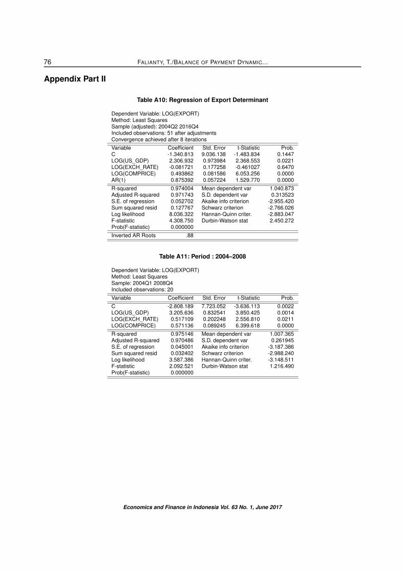
The elasticity of Indonesia’s export to US_GDP ishigher than to commodity prices. In this study, In-donesia’s export is found to be elastic. However,the commodity prices have significantly higher elas-ticity than US_GDP. Felipe et al. (2012) and Felipe,McCombie & Naqvi (2010) stressed the importanceof export elasticity if the country wanted to growfaster without being constrained by the BoP. Wethen checked the progress of Indonesia’s exportelasticity by dividing Export Regression into two pe-riods. The period of global financial crisis is chosenas the structural break for the export regression ofthe changes in export elasticity.

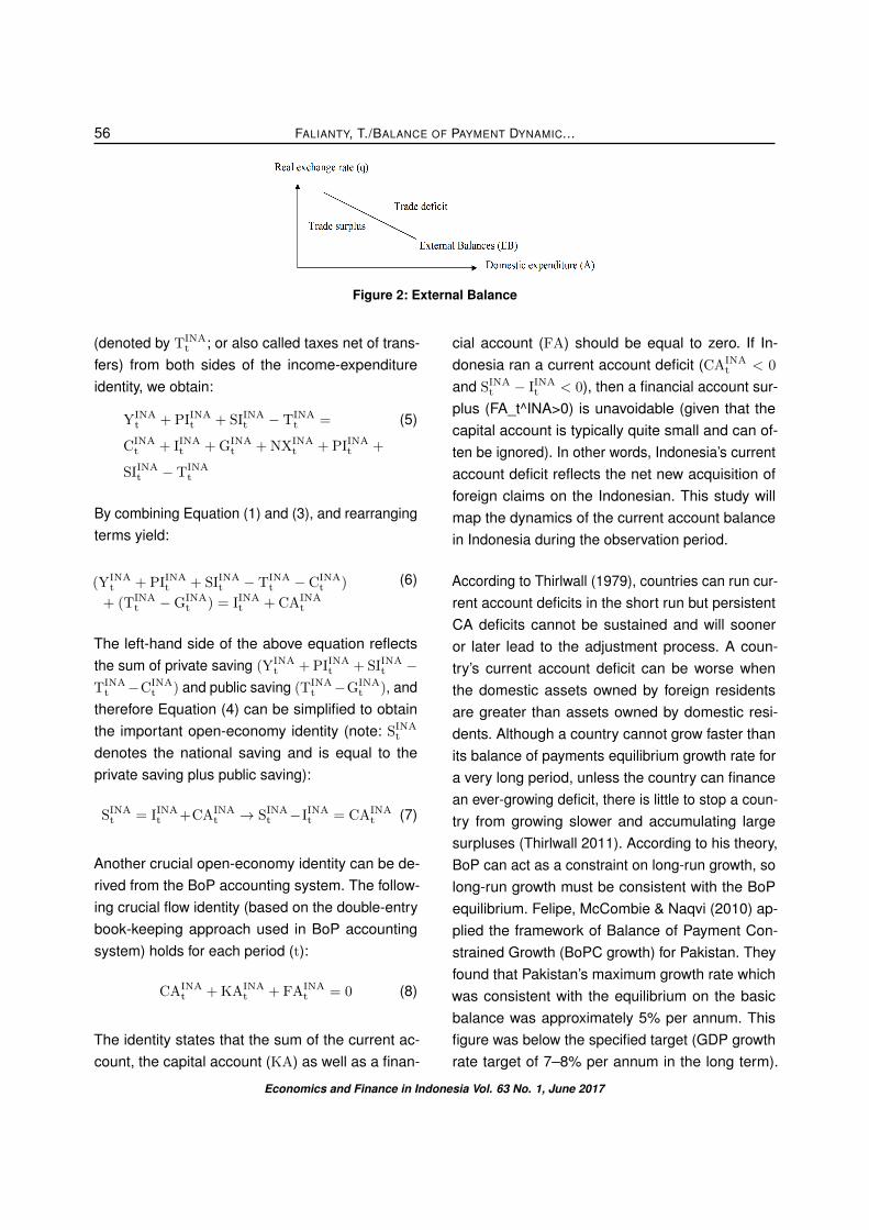
From Table 3 we can conclude that there is no sig-nificant improvement in Indonesia’s export elasticityto World GDP (GDPF). On the other hand, Indone-sia’s export tends to be more elastic to commodityprices (COMPRICE). The export elasticity has in-creased from 0.468 to 0.514 (all coefficients arestatistically significant). Indonesia’s dependence onthe commodity prices can become a constraint inbolstering Indonesian economic growth.

The Figure 6 confirms the significance of the com-modity prices to export. The co-movement of exportand the commodity price index shows that the twovariables are closely related. Athukorala (2006) cre-ated surveys about the trends and patterns of In-donesia’s export performance, focusing specificallyon the comparative experience in major commoditycategories and the changing revealed comparativeadvantage. He examined the implications of China’semergence as a major competitor in the world tradeand explored the factors contributing to the post-crisis export slowdown. His research showed thatIndonesia’s poor export performance in the post-crisis era was largely supply driven.

Referring to Figure 6 and Table 2, the primary in-come has a diverging trend and unit root. The deficit

of primary income has had a tendency to be per-sistent especially since 2008. According to Balanceof Payment Manual 6 from IMF (2010), the primaryincome account shows the primary income flowsbetween resident and nonresident institutions. Pri-mary income represents the return that accrues forinstitutional units for their contribution to the produc-tion process of for the provision of labor, financialassets and renting natural resources to other institu-tional units. Primary income consists of compensa-tion of employees, dividends, reinvested earnings,interest, rent, investment income attributable to pol-icyholders in insurance, standardized guarantees,and pension funds, as well as taxes and subsidieson production and product.

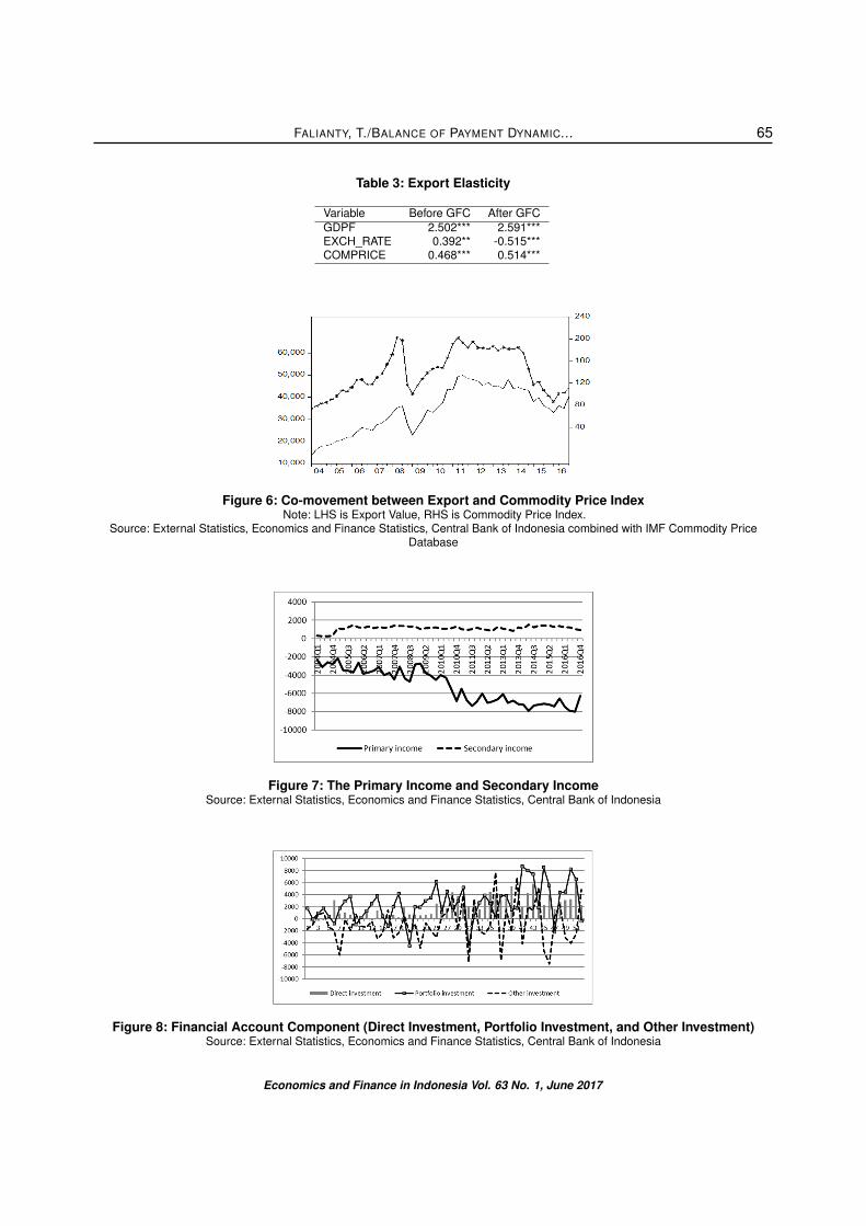
It is a common knowledge that the volatility of portfo-lio investment is higher than the volatility of foreigndirect investment (FDI). It can be seen from theownership composition of Indonesia’s stock mar-ket recorded in C-BEST that foreign investors stilldominate the ownership composition with 64% oftotal ownership. Therefore, Indonesia’s stock mar-ket is very vulnerable to the negative sentiment ofthe global market. The empirical evidence foundon Indonesia’s case is consistent with this state-ment. By referring to Table 2, it can be observedthat the coefficient variation of FDI is lower than thecoefficient variation for portfolio investment. The co-efficient variation of FDI is 0.873, meanwhile, thecoefficient variation of portfolio investment is slightlylarger with 1.196. There are more discussions onfinding the best instruments to finance Indonesia’scurrent account deficits due to the fact that Indone-sia’s current account has suffered from a deficitsince the fourth quarter of 2011. There is a beliefthat the foreign direct investment (FDI) is the bestalternative to finance current account deficit, asidefrom the offshore loans and portfolio investments.However, several studies showed that FDI flowshave apparently contributed to the current accountdeficit in many countries.



Table 3: Export Elasticity

Variable Before GFC After GFCGDPF 2.502*** 2.591***EXCH_RATE 0.392** -0.515***COMPRICE 0.468*** 0.514***

Figure 6: Co-movement between Export and Commodity Price IndexNote: LHS is Export Value, RHS is Commodity Price Index.

Source: External Statistics, Economics and Finance Statistics, Central Bank of Indonesia combined with IMF Commodity PriceDatabase

Figure 7: The Primary Income and Secondary IncomeSource: External Statistics, Economics and Finance Statistics, Central Bank of Indonesia

Figure 8: Financial Account Component (Direct Investment, Portfolio Investment, and Other Investment)Source: External Statistics, Economics and Finance Statistics, Central Bank of Indonesia



The study by Tobing (2014) for Central Bank ofIndonesia working paper showed that from the eco-nomic sector side, imports by the manufacturingsector largely contributed to the current accountdeficit. Hence, it is perceived that in the future theoverall impact of FDI in Indonesia would put morepressures on the deficits of the current accounts.The empirical results using Toda-Yamamoto VARModel shows that there is an evidence to supportthat the capital account affects the current accountboth in the short-run and long-run for Indonesia.Furthermore, there is a one-way causality from FDIto the current account in the short-run and long-run.The results show that FDI has a one-way causalityto the exports, imports, and profit transfers, andthe impact of the causality was dominated more byimports than exports.

Both investment income and employee compen-sation have been widening in term of the deficit.Indonesia’s current account deficit is structurallyaffected by the increasing outflow of investmentincome and employee compensation. By usingGranger Causality Test, we also found the evidencefor the significance of FDI to Indonesia’s currentaccount with 4 lags. FDI (-4) has a significant andnegative effect on the current account. (The resultscan be seen in Appendix).

Regarding the BoP analysis and the current ac-count sustainability, we should take a look at the NetInternational Investment Position (NIIP). In Equa-tion (12), NIIP is equal to the present value of futuretrade balances. If NIIPt < 0, then at some pointin the future the economy is expected to generatesufficient trade surpluses to pay off the initial foreigndebt. So, one of important homework for Indonesiais to create sufficient trade surplus. According toEquation (12), Figure 9, and the result in Table 1, torecover NIIP to its equilibrium level we need to boostexport over import. Trade surplus could increasethe net foreign asset holding (note NIIP). Besidesboosting export, Indonesia also should increase the

primary income inflows (The net international invest-ment position provides a measure of net financialclaims with nonresidents in addition to using goldbullion as monetary gold. If BoP is a flow concept,NIIP is a stock concept). According to BoP and IIPmanual of IMF (2010), The international investmentposition (IIP) is a statistical statement that showsat a point in time the value and composition of (a)financial assets of residents of an economy thatare claims on nonresidents and gold bullion heldas reserve assets, and (b) liabilities of residents ofan economy to nonresidents.. The difference be-tween an economy’s external financial assets andliabilities is the economy’s net IIP, which might bepositive or negative.

4.1. Balance of Payment ConstrainedGrowth (BOPC Growth)

From the steps described in the methodology sec-tion, we managed to obtain the BOPC growth inFigure 10. It can be observed that BOPC growth de-clined dramatically in the period of 2011–2015. After2015, BOPC growth has recovered to the normaltrend. The balance of payment condition generallyaffects Indonesia’s economic growth. The explana-tion of BOPC growth is in line with the decliningtrade balance and the persistence of primary in-come deficit since 2011. Therefore, we can con-clude that one of the main constraints on Indone-sia’s economic growth is its economic structurewhich is specifically represented in BoP compo-nents (export that depends on primary commodityand persistence of primary income deficit).

5. Conclusions

Understanding the dynamics of the BoP and itscomponents can help policymakers in designing a



Figure 9: Primary Income (Employee Compensation and Investment Income)Source: External Statistics, Economics and Finance Statistics, Central Bank of Indonesia

Figure 10: Net International Investment Position of IndonesiaSource: External Statistics, Economics and Finance Statistics, Central Bank of Indonesia

Figure 11: Balance of Payment Constrained Growth EstimationSource: Estimated from Equation (19)



policy to maintain the BoP stability and achieve theexternal balances. There are three parts of the con-clusion that can be derived from this study. The firstconclusion is that the current account componentbehavior, BoP, secondary income, and financial ac-count are found to be stationary which means thedata are mean reverting. On the other hand, thecurrent account balance, trade balance, service bal-ance, primary income and capital account balanceare non-reverting and persistent. In the more de-tailed BoP components, it is observed that there arehighly persistent components of BoP, which are oiland gas (goods category), travel, intellectual prop-erty, telecommunication, computer, and information,personal, cultural, recreational services (servicescategory), investment income and employee com-pensation (primary income), and general govern-ment (secondary income category). The secondconclusion is that all the components of the financialaccount are mean reverting. The third conclusionexplains two important pieces of evidence in thecurrent account and financial account. First the evi-dence of the importance of the commodity prices toexport rate (as expected in the hypothesis). Second,the persistence of the primary income deficit relatedto the side effect of FDI (financial account) as asource of financing for the current account deficit.Both of the evidence can create a constraint onIndonesia’s economic growth. To improve Indone-sia’s economic growth (with the framework of BOPCgrowth), Indonesia should improve the dependencyof its export of primary commodities and Indonesiashould focus on reducing its primary income deficit.

References

[1] Andaiyani, S & Falianty, TA 2017, ’ASEAN Credit GrowthAnd Asset Price Response to Global Financial Cycle’, Bul-letin of Monetary Economics and Banking, vol. 20, no. 2,pp. 203–228.

[2] Asmarani, T & Falianty, T 2014,’The Persistency and TheSustainability of Indonesia’s Current Acount Deficit’, Bul-

letin of Monetary Economics and Banking, vol. 17, no. 3,pp. 316–336.

[3] Athukorala, C 2006, ’Post-crisis export performance: TheIndonesian Experience in Regional Perspective’, Bulletinof Indonesian Economic Studies, vol. 42, pp. 3–28.

[4] Calderon, C, Chong A, & Loayza, N 1999, ’Determinants ofCurrent Account Deficits in Developing Countries’, CentralBank of Chile Working Papers No. 51.

[5] Chen, S-W 2011, ’Current Account Deficits and Sustain-ability: Evidence from the OECD Countries’, EconomicModelling, vol. 28, no. 4, pp. 1455–1464.

[6] Central Bank of Indonesia 2016, ’Current Account Sus-tainability: Capital and Financial Transaction’, unpublishedpaper.

[7] Clower, E & Ito, H 2012, ’The Persistence of Current Ac-count Balances and Its Determinants’, ADBI Working PaperSeries 400.

[8] Falianty, T 2015, ’Exchange Rate Effect on Indonesian Ex-port: Comparisons of Two Crises Episodes’, InternationalJournal of Economic Research, vol. 6, no. 6, pp. 60–75.

[9] Felipe, J & Lanzafame, M 2017, ’Balance of Payment Con-strained Growth Rate’, presented at Workshop on PotentialGrowth, Jakarta, Indonesia June 8–9, 2017.

[10] Felipe, J, McCombie, JSL, & Naqvi, K 2010, ’Is Pakistan’sGrowth Rate Balance of Payment Constrained? Policiesand Implications for Development and Growth’, Oxford De-velopment Studies, vol 38, no. 4.

[11] Felipe, J, Kumar, U, Abdon, A & Bacate, M 2012, ’Prod-uct Complexity and Economic Development’, StructuralChange and Economic Dynamics, vol. 23, no. 1, pp. 36–68.

[12] Freytag, A 2008, ’Balance of Payment Dynamic, Institutionand Economic Performance in South Africa a Policy Ori-ented Study’, Trade and Industrial Policy Studies WorkingPaper Series 2008-04.

[13] IMF 2010, Balance of Payment and International Invest-ment Position Manual, 6th ed, International Monetary Fund,Washington.

[14] IMF 2016, ’Too Slow for Too Long’, World Economic Out-look, April 2016, International Monetary Fund.

[15] Jaffri, AA, Asghar, N, Ali, MM & Asjed, R 2012, ’Foreign Di-rect Investment and Current Account Balance of Pakistan’,Pakistan Economic and Social Review, vol. 50, no. 2, pp.207–222.

[16] Kumar, A 2007, ’Does foreign direct investment help emerg-ing economies?’, Economic Letter: Federal Reserve Bankof Dallas, vol. 2, no. 1, pp. 1–8.

[17] Krugman, P & Obstfeld, M 2003, International Economics6th Edition, Pearson.

[18] MacKinnon, JG 1996, ’Numerical Distribution Functionsfor Unit Root and Cointegration Tests’, Journal of AppliedEconometrics, vol.11, no. 6, pp. 601–618.



[19] Obstfeld, M & Rogoff, K 1996, Foundation of InternationalMacroeconomics, Cambridge, MA: MIT.

[20] Sastre, L 2015, ’Exchange Rate, Cross Elasticities Be-tween Exports and Imports and Current Account Sus-tainability: The Spanish Case’, Review Economics andFinance, pp. 32–46.

[21] Senhadji, A & Montenegro, C 1998, ’Time Series Analysisof Export Demand Equations: A Cross Country Analysis’,IMF Working Paper/98/149, pp. 5–7.

[22] Thirlwall, AP 1979, ’The Balance of Payments Constrain asan Explanation of International Growth Differences’, BancaNazionale del Lavoro Quarterly Review, vol. 32, no. 28.

[23] Thirlwall, AP 2011, Economics of Development, PalgraveMacMillan, UK

[24] Tobing, L 2014, ’Current Account Deficit Sustainability: Fi-nancing Through Capital and Financial Account’, BankIndonesia Working Paper No. 72.

[25] Tsen, W 2014, ’External Balance and Budget in Malaysia’,AAMJAF, vol. 10, no. 2, pp. 37–54

[26] World Bank 2017, ’Sustaining Reform Momentum’, Indone-sia Economic Quarterly.



Appendix

Appendix Part I

Table A1: BOP unit root test

Null Hypothesis: BOP has a unit rootExogenous: ConstantLag Length: 0 (Automatic based on SIC, MAXLAG=10)

t-Statistic Prob.*Augmented Dickey-Fuller test statistic -4.484.574 0.0007Test critical values: 1% level -3.565.430

5% level -2.919.95210% level -2.597.905

*MacKinnon (1996) one-sided p-values.

Augmented Dickey-Fuller Test EquationDependent Variable: D(BOP)Included observations: 51 after adjustmentsVariable Coefficient Std. Error t-Statistic Prob.BOP(-1) -0.586166 0.130707 -4.484.574 0.0000C 1.157.210 5.646.049 2.049.592 0.0458R-squared 0.291000 Mean dependent var 6.181.176Adjusted R-squared 0.276530 S.D. dependent var 4.273.879S.E. of regression 3.635.234 Akaike info criterion 1.927.316Sum squared resid 6.48E+08 Schwarz criterion 1.934.892Log likelihood -4.894.656 Hannan-Quinn criter. 1.930.211F-statistic 2.011.140 Durbin-Watson stat 2.056.728Prob(F-statistic) 0.000044



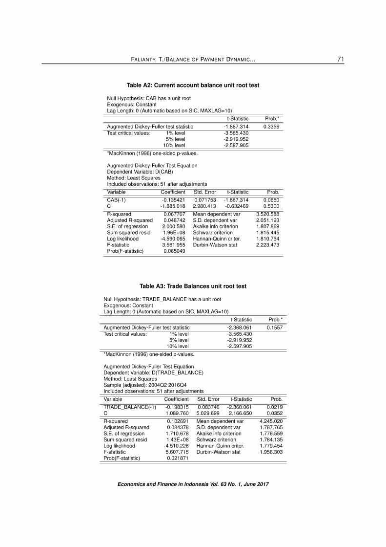
Table A2: Current account balance unit root test

Null Hypothesis: CAB has a unit rootExogenous: ConstantLag Length: 0 (Automatic based on SIC, MAXLAG=10)


5% level -2.919.95210% level -2.597.905


Augmented Dickey-Fuller Test EquationDependent Variable: D(CAB)Method: Least SquaresIncluded observations: 51 after adjustmentsVariable Coefficient Std. Error t-Statistic Prob.CAB(-1) -0.135421 0.071753 -1.887.314 0.0650C -1.885.018 2.980.413 -0.632469 0.5300R-squared 0.067767 Mean dependent var 3.520.588Adjusted R-squared 0.048742 S.D. dependent var 2.051.193S.E. of regression 2.000.580 Akaike info criterion 1.807.869Sum squared resid 1.96E+08 Schwarz criterion 1.815.445Log likelihood -4.590.065 Hannan-Quinn criter. 1.810.764F-statistic 3.561.955 Durbin-Watson stat 2.223.473Prob(F-statistic) 0.065049

Table A3: Trade Balances unit root test

Null Hypothesis: TRADE_BALANCE has a unit rootExogenous: ConstantLag Length: 0 (Automatic based on SIC, MAXLAG=10)


5% level -2.919.95210% level -2.597.905


Augmented Dickey-Fuller Test EquationDependent Variable: D(TRADE_BALANCE)Method: Least SquaresSample (adjusted): 2004Q2 2016Q4Included observations: 51 after adjustmentsVariable Coefficient Std. Error t-Statistic Prob.TRADE_BALANCE(-1) -0.198315 0.083746 -2.368.061 0.0219C 1.089.760 5.029.699 2.166.650 0.0352R-squared 0.102691 Mean dependent var 4.245.020Adjusted R-squared 0.084378 S.D. dependent var 1.787.765S.E. of regression 1.710.678 Akaike info criterion 1.776.559Sum squared resid 1.43E+08 Schwarz criterion 1.784.135Log likelihood -4.510.226 Hannan-Quinn criter. 1.779.454F-statistic 5.607.715 Durbin-Watson stat 1.956.303Prob(F-statistic) 0.021871



Table A4: Service Balances

Null Hypothesis: SERVICES_BALANCE has a unit rootExogenous: ConstantLag Length: 3 (Automatic based on SIC, MAXLAG=10)

t-Statistic Prob.*Augmented Dickey-Fuller test statistic -0.987669 0.7505Test critical values: 1% level -3.574.446

5% level -2.923.78010% level -2.599.925


Augmented Dickey-Fuller Test EquationDependent Variable: D(SERVICES_BALANCE)Method: Least SquaresSample (adjusted): 2005Q1 2016Q4Included observations: 48 after adjustmentsVariable Coefficient Std. Error t-Statistic Prob.SERVICES_BALANCE(-1) -0.169875 0.171996 -0.987669 0.3288D(SERVICES_BALANCE(-1)) -0.531946 0.176483 -3.014.148 0.0043D(SERVICES_BALANCE(-2)) -0.351565 0.166908 -2.106.336 0.0410D(SERVICES_BALANCE(-3)) -0.433374 0.138884 -3.120.396 0.0032C -4.307.596 4.661.394 -0.924100 0.3606R-squared 0.454160 Mean dependent var 1.419.896Adjusted R-squared 0.403385 S.D. dependent var 7.416.255S.E. of regression 5.728.381 Akaike info criterion 1.563.742Sum squared resid 14110172 Schwarz criterion 1.583.233Log likelihood -3.702.980 Hannan-Quinn criter. 1.571.108F-statistic 8.944.427 Durbin-Watson stat 1.660.809Prob(F-statistic) 0.000024



Table A5: Primary income

Null Hypothesis: PRIMARY_INCOME has a unit rootExogenous: ConstantLag Length: 4 (Automatic based on SIC, MAXLAG=10)


5% level -2.925.16910% level -2.600.658


Augmented Dickey-Fuller Test EquationDependent Variable: D(PRIMARY_INCOME)Method: Least SquaresSample (adjusted): 2005Q2 2016Q4Included observations: 47 after adjustmentsVariable Coefficient Std. Error t-Statistic Prob.PRIMARY_INCOME(-1) -0.072818 0.057111 -1.275.032 0.2095D(PRIMARY_INCOME(-1)) -0.442155 0.157214 -2.812.440 0.0075D(PRIMARY_INCOME(-2)) -0.361597 0.169989 -2.127.179 0.0395D(PRIMARY_INCOME(-3)) -0.185434 0.169245 -1.095.656 0.2796D(PRIMARY_INCOME(-4)) 0.321472 0.152773 2.104.254 0.0415C -5.595.893 3.176.859 -1.761.454 0.0856R-squared 0.418746 Mean dependent var -8.725.340Adjusted R-squared 0.347861 S.D. dependent var 8.226.043S.E. of regression 6.642.951 Akaike info criterion 1.595.407Sum squared resid 18092809 Schwarz criterion 1.619.026Log likelihood -3.689.207 Hannan-Quinn criter. 1.604.295F-statistic 5.907.422 Durbin-Watson stat 1.911.301Prob(F-statistic) 0.000336

Table A6: Secondary income

Null Hypothesis: SECONDARY_INCOME has a unit rootExogenous: ConstantLag Length: 0 (Automatic based on SIC, MAXLAG=10)


5% level -2.919.95210% level -2.597.905


Augmented Dickey-Fuller Test EquationDependent Variable: D(SECONDARY_INCOME)Method: Least SquaresSample (adjusted): 2004Q2 2016Q4Included observations: 51 after adjustmentsVariable Coefficient Std. Error t-Statistic Prob.SECONDARY_INCOME(-1) -0.320499 0.088714 -3.612.703 0.0007C 3.718.315 1.026.493 3.622.349 0.0007R-squared 0.210335 Mean dependent var 1.259.902Adjusted R-squared 0.194219 S.D. dependent var 2.027.323S.E. of regression 1.819.832 Akaike info criterion 1.328.413Sum squared resid 1622777. Schwarz criterion 1.335.989Log likelihood -3.367.454 Hannan-Quinn criter. 1.331.308F-statistic 1.305.163 Durbin-Watson stat 2.392.005Prob(F-statistic) 0.000713



Table A7: Capital Financial

Null Hypothesis: CAPITAL_FINANCIAL has a unit rootExogenous: ConstantLag Length: 1 (Automatic based on SIC, MAXLAG=10)


5% level -2.921.17510% level -2.598.551


Augmented Dickey-Fuller Test EquationDependent Variable: D(CAPITAL_FINANCIAL)Method: Least SquaresSample (adjusted): 2004Q3 2016Q4Included observations: 50 after adjustmentsVariable Coefficient Std. Error t-Statistic Prob.CAPITAL_FINANCIAL(-1) -0.403185 0.157121 -2.566.074 0.0135D(CAPITAL_FINANCIAL(-1)) -0.445082 0.131604 -3.381.979 0.0015C 1.743.728 8.234.104 2.117.690 0.0395R-squared 0.492225 Mean dependent var 1.738.610Adjusted R-squared 0.470617 S.D. dependent var 5.876.863S.E. of regression 4.275.927 Akaike info criterion 1.961.751Sum squared resid 8.59E+08 Schwarz criterion 1.973.224Log likelihood -4.874.379 Hannan-Quinn criter. 1.966.120F-statistic 2.278.034 Durbin-Watson stat 1.991.450Prob(F-statistic) 0.000000

Table A8: Capital

Null Hypothesis: CAPITAL_ACC has a unit rootExogenous: ConstantLag Length: 3 (Automatic based on SIC, MAXLAG=9)


5% level -2.933.15810% level -2.604.867


Augmented Dickey-Fuller Test EquationDependent Variable: D(CAPITAL_ACC)Method: Least SquaresIncluded observations: 42 after adjustmentsVariable Coefficient Std. Error t-Statistic Prob.CAPITAL_ACC(-1) -0.159751 0.125913 -1.268.746 0.2125D(CAPITAL_ACC(-1)) -0.503858 0.165213 -3.049.742 0.0042D(CAPITAL_ACC(-2)) -0.683219 0.124991 -5.466.137 0.0000D(CAPITAL_ACC(-3)) -0.350646 0.136230 -2.573.935 0.0142C 0.025995 7.589.292 0.003425 0.9973R-squared 0.574269 Mean dependent var -1.591.667Adjusted R-squared 0.528244 S.D. dependent var 5.269.050S.E. of regression 3.619.022 Akaike info criterion 1.012.680Sum squared resid 48460.10 Schwarz criterion 1.033.366Log likelihood -2.076.628 Hannan-Quinn criter. 1.020.262F-statistic 1.247.731 Durbin-Watson stat 1.773.626Prob(F-statistic) 0.000002



Table A9: Financial

Null Hypothesis: FINANCIAL has a unit rootExogenous: ConstantLag Length: 1 (Automatic based on SIC, MAXLAG=10)


5% level -2.921.17510% level -2.598.551


Augmented Dickey-Fuller Test EquationDependent Variable: D(FINANCIAL)Method: Least SquaresSample (adjusted): 2004Q3 2016Q4Included observations: 50 after adjustmentsVariable Coefficient Std. Error t-Statistic Prob.FINANCIAL(-1) -0.397470 0.156271 -2.543.464 0.0143D(FINANCIAL(-1)) -0.446981 0.131538 -3.398.103 0.0014C 1.708.426 8.175.177 2.089.772 0.0421R-squared 0.490082 Mean dependent var 1.738.610Adjusted R-squared 0.468383 S.D. dependent var 5.865.264S.E. of regression 4.276.486 Akaike info criterion 1.961.778Sum squared resid 8.60E+08 Schwarz criterion 1.973.250Log likelihood -4.874.444 Hannan-Quinn criter. 1.966.146F-statistic 2.258.581 Durbin-Watson stat 1.992.015Prob(F-statistic) 0.000000



Appendix Part II

Table A10: Regression of Export Determinant

Dependent Variable: LOG(EXPORT)Method: Least SquaresSample (adjusted): 2004Q2 2016Q4Included observations: 51 after adjustmentsConvergence achieved after 8 iterationsVariable Coefficient Std. Error t-Statistic Prob.C -1.340.813 9.036.138 -1.483.834 0.1447LOG(US_GDP) 2.306.932 0.973984 2.368.553 0.0221LOG(EXCH_RATE) -0.081721 0.177258 -0.461027 0.6470LOG(COMPRICE) 0.493862 0.081586 6.053.256 0.0000AR(1) 0.875392 0.057224 1.529.770 0.0000R-squared 0.974004 Mean dependent var 1.040.873Adjusted R-squared 0.971743 S.D. dependent var 0.313523S.E. of regression 0.052702 Akaike info criterion -2.955.420Sum squared resid 0.127767 Schwarz criterion -2.766.026Log likelihood 8.036.322 Hannan-Quinn criter. -2.883.047F-statistic 4.308.750 Durbin-Watson stat 2.450.272Prob(F-statistic) 0.000000Inverted AR Roots .88

Table A11: Period : 2004–2008

Dependent Variable: LOG(EXPORT)Method: Least SquaresSample: 2004Q1 2008Q4Included observations: 20Variable Coefficient Std. Error t-Statistic Prob.C -2.808.189 7.723.052 -3.636.113 0.0022LOG(US_GDP) 3.205.636 0.832541 3.850.425 0.0014LOG(EXCH_RATE) 0.517109 0.202248 2.556.810 0.0211LOG(COMPRICE) 0.571136 0.089245 6.399.618 0.0000R-squared 0.975146 Mean dependent var 1.007.365Adjusted R-squared 0.970486 S.D. dependent var 0.261945S.E. of regression 0.045001 Akaike info criterion -3.187.386Sum squared resid 0.032402 Schwarz criterion -2.988.240Log likelihood 3.587.386 Hannan-Quinn criter. -3.148.511F-statistic 2.092.521 Durbin-Watson stat 1.216.490Prob(F-statistic) 0.000000



Table A12: Period: 2009–2016

Dependent Variable: LOG(EXPORT)Method: Least SquaresSample: 2009Q1 2016Q4Included observations: 32Variable Coefficient Std. Error t-Statistic Prob.C -2.208.375 2.261.520 -9.765.005 0.0000LOG(US_GDP) 3.665.103 0.328538 1.115.581 0.0000LOG(EXCH_RATE) -0.587637 0.117446 -5.003.480 0.0000LOG(COMPRICE) 0.553205 0.046879 1.180.064 0.0000R-squared 0.950137 Mean dependent var 1.059.046Adjusted R-squared 0.944794 S.D. dependent var 0.187832S.E. of regression 0.044133 Akaike info criterion -3.286.758Sum squared resid 0.054536 Schwarz criterion -3.103.541Log likelihood 5.658.812 Hannan-Quinn criter. -3.226.026F-statistic 1.778.454 Durbin-Watson stat 1.739.966Prob(F-statistic) 0.000000



Appendix Part III

Granger Causality Test

Table A13: Foreign Direct Investment

VEC Granger Causality/Block Exogeneity Wald TestsSample: 2004Q1 2016Q4Included observations: 47Dependent variable: D(FDI)Excluded Chi-sq df Prob.D(CAB) 4.326778 4 0.3636All 4.326778 4 0.3636Dependent variable: D(CAB)Excluded Chi-sq df Prob.D(FDI) 6.704485 4 0.1524All 6.704485 4 0.1524

Table A14: Portfolio Investment

VEC Granger Causality/Block Exogeneity Wald TestsSample: 2004Q1 2016Q4Included observations: 47Dependent variable: D(PORTFOLIO)Excluded Chi-sq df Prob.D(CAB) 5.376025 4 0.2508All 5.376025 4 0.2508Dependent variable: D(CAB)Excluded Chi-sq df Prob.D(PORTFOLIO) 6.930886 4 0.1396All 6.930886 4 0.1396



Table A15: FDI

Dependent Variable: CABSample (adjusted): 2005Q1 2016Q4Included observations: 48 after adjustmentsVariable Coefficient Std. Error t-Statistic Prob.C 3.685.777 6.107.194 0.603514 0.5494FDI(-1) 0.252353 0.231045 1.092.222 0.2810FDI(-2) -0.030854 0.235998 -0.130740 0.8966FDI(-3) -0.248067 0.230295 -1.077.170 0.2876FDI(-4) -0.419154 0.227582 -1.841.770 0.0726CAB(-1) 0.772275 0.109122 7.077.186 0.0000R-squared 0.792036 Mean dependent var -1.576.908Adjusted R-squared 0.767278 S.D. dependent var 4.006.568S.E. of regression 1.932.819 Akaike info criterion 1.808.781Sum squared resid 1.57E+08 Schwarz criterion 1.832.172Log likelihood -4.281.076 Hannan-Quinn criter. 1.817.621F-statistic 3.199.156 Durbin-Watson stat 2.290.260Prob(F-statistic) 0.000000

Dependent Variable: FDISample (adjusted): 2005Q1 2016Q4Included observations: 48 after adjustmentsVariable Coefficient Std. Error t-Statistic Prob.C 1.585.746 3.478.655 4.558.504 0.0000CAB(-1) -0.307484 0.112134 -2.742.106 0.0089CAB(-2) 0.093283 0.128114 0.728128 0.4706CAB(-3) 0.050500 0.125832 0.401330 0.6902CAB(-4) -0.043525 0.102284 -0.425534 0.6726FDI(-1) 0.126344 0.163023 0.775009 0.4427R-squared 0.398614 Mean dependent var 2.184.153Adjusted R-squared 0.327021 S.D. dependent var 1.656.116S.E. of regression 1.358.599 Akaike info criterion 1.738.276Sum squared resid 77523287 Schwarz criterion 1.761.667Log likelihood -4.111.864 Hannan-Quinn criter. 1.747.116F-statistic 5.567.742 Durbin-Watson stat 2.043.531Prob(F-statistic) 0.000506



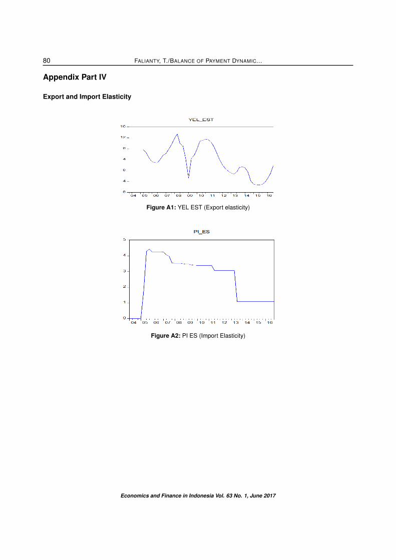
Appendix Part IV

Export and Import Elasticity

Figure A1: YEL EST (Export elasticity)

Figure A2: PI ES (Import Elasticity)


Balance of Payment Dynamic in Indonesia and

Documents

Transcript of Balance of Payment Dynamic in Indonesia and