Backward generalizations of PCA for shape representations · IntroductionPCA GeneralizationS-reps...
33
Introduction PCA Generalization S-reps and CPNS Backward generalizations of PCA for shape representations Sungkyu Jung University of Pittsburgh BIRS–Geometry for Anatomy Presentation based on Joint work with Dibyendusekhar Goswami, J¨ orn Schultz, Xiaoxiao Liu, Ritwik Chaudhuri, Steve Marron, Ian Dryden, Steve Pizer 1 / 33
Transcript of Backward generalizations of PCA for shape representations · IntroductionPCA GeneralizationS-reps...

Introduction PCA Generalization S-reps and CPNS
Backward generalizations of PCAfor shape representations
Sungkyu JungUniversity of Pittsburgh
BIRS–Geometry for Anatomy
Presentation based on Joint work with DibyendusekharGoswami, Jorn Schultz, Xiaoxiao Liu, Ritwik Chaudhuri, Steve
Marron, Ian Dryden, Steve Pizer
1 / 33

Introduction PCA Generalization S-reps and CPNS
Principal Component Analysis (PCA)
1. Study population of shape representations
2. Exploratory statistics- Visualization of data structure
3. Dimension reduction and Estimation of Probability distribution
Generalization of PCA to shape representations
• Shape representations are either spheres, quotient of spheres,or involve position-tuples, directions, and (log) sizes
• PCA suited for this type of manifolds
More details on skeletal models (Pizer)
Models of object interiors designed for probability distributionestimation: s-reps
2 / 33
Introduction PCA Generalization S-reps and CPNS
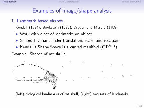
Examples of image/shape analysis
1. Landmark based shapes
Kendall (1984), Bookstein (1986), Dryden and Mardia (1998)
• Work with a set of landmarks on object
• Shape: Invariant under translation, scale, and rotation
• Kendall’s Shape Space is a curved manifold (CPk−2)
Example: Shapes of rat skulls
(left) biological landmarks of rat skull, (right) two sets of landmarks
3 / 33
Introduction PCA Generalization S-reps and CPNS
Examples of image/shape analysis
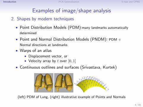
2. Shapes by modern techniques
• Point Distribution Models (PDM):many landmarks automatically
determined
• Point and Normal Distribution Models (PNDM): PDM +
Normal directions at landmarks
• Warps of an atlas• Displacement vector, or• Velocity array by t over [0, 1]
• Continuous outlines and surfaces (Srivastava, Kurtek)
(left) PDM of Lung, (right) illustrative example of Points and Normals
4 / 33

Introduction PCA Generalization S-reps and CPNS
Examples of image/shape analysis
3. Skeletal representations (s-rep)
Siddiqi and Pizer (2008), Pizer et al. (2011)
• Special case: Medial representations (m-rep)
• Capturing interior of objects
• Suitable for statistical analysis
• More details covered in Pizer’s talk
medial atom, slabular m-rep model, slabular s-rep, quasi-tubular s-rep,
multi-object5 / 33

Introduction PCA Generalization S-reps and CPNS
Two equivalent formulations of Euclidean PCAForward stepwise view of PCA: center point - line - plane - ...
Backward stepwise view of PCA:
1. Begin with full data space (Rd)
2. Find d− 1 dim’l affine subspace (best approximates data)
3. Reduce dimension further to d− 2, d− 3, . . . , 0.
Euclidean case: Forward PCA = Backward PCA6 / 33

Introduction PCA Generalization S-reps and CPNS
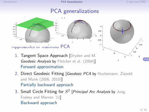
PCA generalizations
Complications on manifolds
• Orthogonal lines → Orthogonal geodesics
• Need to find an appropriate ‘mean’
Approaches of manifold PCA
1. Tangent Space Approach [Dryden and Mardia (1998), Principal
Geodesic Analysis by Fletcher et al. (2004)]
Forward approximation
2. Direct Geodesic Fitting [Geodesic PCA by Huckemann, Ziezold
and Munk (2006, 2010)]
Partially backward approach
3. Small Circle Fitting for S2 [Principal Arc Analysis by Jung,
Foskey and Marron ’11]
Backward approach
7 / 33
Introduction PCA Generalization S-reps and CPNS
PCA generalizations
Complications on manifolds
• Orthogonal lines → Orthogonal geodesics
• Need to find an appropriate ‘mean’
Approaches of manifold PCA
1. Tangent Space Approach [Dryden and Mardia (1998), Principal
Geodesic Analysis by Fletcher et al. (2004)]
Forward approximation
2. Direct Geodesic Fitting [Geodesic PCA by Huckemann, Ziezold
and Munk (2006, 2010)]
Partially backward approach
3. Small Circle Fitting for S2 [Principal Arc Analysis by Jung,
Foskey and Marron ’11]
Backward approach
8 / 33
Details

Introduction PCA Generalization S-reps and CPNS
Analysis of Principal Nested Spheres
Jung, Dryden and Marron ’11
• Generalization of Principal Arc Analysis to Sd, d ≥ 2.
• Decomposition of Sd captures non-geodesic variation in lowerdimensional spheres.
• Ak: k-dimensional Principal Nested Sphere (PNS)
A0 ⊂ A1 ⊂ · · · ⊂ Ad−1 ⊂ Sd.
• Works for Kendall’s landmark shape data through thepreshape space Sd.
• Fitted in backward stepwise fashion.
9 / 33

Introduction PCA Generalization S-reps and CPNS
Sequence of Principal Nested Spheres
Begin with x1, . . . ,xn ∈ Sd
1. Fit Ad−1∼= (d− 1)-sphere
• best non-geodesic (d-1) dim’l approximation
2. Fit Ad−2∼= (d− 2)-sphere
...
3. Reach A0 (PNSmean)
4. Result in A0 ⊂ A1 ⊂ · · · ⊂ Ad−1 ⊂ Sd
10 / 33

Introduction PCA Generalization S-reps and CPNS
Best fitting subsphere
• Samples: x1, . . . ,xn ∈ Sd
• Subsphere: Ad−1(v1, r1) ⊂ Sd
• Residual ξ of x from a subsphere Ad−1
- Signed length of the minimal geodesic that joins x to Ad−1.
Subsphere fitting
Ad−1 ≡ Ad−1(v1, r1) minimizes the sum of squared residuals
n∑i=1
ξi(v1, r1)2 =
n∑i=1
{ρd(xi,v1)− r1}2,
among all v1 ∈ Sd, r1 ∈ (0, π/2]. Detail....
11 / 33
Introduction PCA Generalization S-reps and CPNS
Byproducts of PNS
Euclidean-Type Representation (Principal Scores matrix)
• Stacked residuals from each layer
• Analogue of principal component scores
• Used to visualize the data, and for further analysis
% Variance explained
• Sample variance of residuals (from each layer) over the sum ofall variances
Principal Arc
• the direction of major variations defined by PNS
12 / 33

Introduction PCA Generalization S-reps and CPNS
A special case: PNG
A great sphere is a sphere with radius 1 (or r = π/2).Interesting & important special case of PNS:
Principal Nested Great Spheres (PNG)
• Setting r = π/2 for each subsphere fitting.
• Principal arcs become great circles (i.e. geodesics).
• The principal geodesics, found by PNG, are similar to thegeodesic-based PCs.
• Close to the Geodesic PCA (direct geodesic fitting) than thetangent space approach.
13 / 33
Introduction PCA Generalization S-reps and CPNS
Choice between small and great sphere
1. Strictly using small spheres (PNS) —nongeodesic decomp.
2. Adopted tests:H0 : Great Sphere (r = π/2) vs H1 : Small sphere
(r < π/2).
3. Strictly using great Spheres (PNG) —geodesic decomp.
4. Soft decision between small and great sphere. —Ongoingwork.
14 / 33

Introduction PCA Generalization S-reps and CPNS
Choice between small and great sphere
1. Strictly using small spheres (PNS) —nongeodesic decomp.
2. Adopted tests:H0 : Great Sphere (r = π/2) vs H1 : Small sphere
(r < π/2).
3. Strictly using great Spheres (PNG) —geodesic decomp.
4. Soft decision between small and great sphere. —Ongoingwork.
15 / 33

Introduction PCA Generalization S-reps and CPNS
Kendall’s 2D landmark shape space
Planar shape space Σk2
• A shape is a point in Kendall’s shape space with dimension2k − 2− 1− 1
Preshape space Sk2 ∼= Sd
• Preshape is what is left from removing location and scale• Dimensionality of preshape space is d = 2k − 2− 1
PNS to shape data
• Desire that Ad−1 of Sd leaves zero residuals.
• Achieved when each shape is aligned to a common base shape(e.g. Procrustes mean)
16 / 33

Introduction PCA Generalization S-reps and CPNS
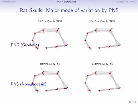
Example: Shape of Rat Skulls
- Shape data with 8 landmarks on plane in Σ82
• Non-geodesic variation captured by PNS (and not by PNG)
• Scatterplot given by Principal Scores
• Shape changes related to growth of rats.
17 / 33
Introduction PCA Generalization S-reps and CPNS
Rat Skulls: Major mode of variation by PNS
1st Princ. Geod by PNGS 2nd Princ. Geod by PNGS
1st Princ. Arc by PNS 2nd Princ. Arc by PNS
18 / 33
PNG (Geodesic)
PNS (Non-geodesic)

Introduction PCA Generalization S-reps and CPNS
Rat Skulls: Scatterplots
−0.1 −0.05 0 0.05 0.1
−0.04
−0.02
0
0.02
0.04
PNG 1, 82.22%
PN
G 2
, 7.
77%
(a)
−0.1 −0.05 0 0.05 0.1
−0.03
−0.02
−0.01
0
0.01
0.02
0.03
PNG 1, 82.22%
PN
G 3
, 2.
47%
(b)
−0.15 −0.1 −0.05 0 0.05 0.1
−0.02
0
0.02
0.04
PNS 1, 88.67%
PN
S 2
, 3.
31%
(c)
−0.15 −0.1 −0.05 0 0.05 0.1
900
1000
1100
1200
1300
1400
1500
PNS 1
cent
roid
siz
e
(d)
day 7
1421
3040
60
90
150
• PNS need 1 mode (PNG need 2 modes) to capture thenon-geodesic variation
• Shape change by growth of rats explained by PNS 1• PNS 1 linearly correlated with size of skulls (R = 0.9705)
19 / 33
PNG →
PNS →

Introduction PCA Generalization S-reps and CPNS
CPNS on Lung Respiratory MotionJung, Liu, Pizer and Marron ’10
• PDM represents shape of human lung, pre-aligned with Npoints- Scaled PDM is ∈ S3N−1
- Size variable is ∈ R+
• PDM in R3N = ScaledPDM ⊕ Size ∈ S3N−1 ⊗ R+
- Thus want composite of PNS (S3N−1) and R1.
20 / 33

Introduction PCA Generalization S-reps and CPNS
Composite PNS for PDM
Must capture correlations between Euclidean and non-Euclideanfeatures
21 / 33

Introduction PCA Generalization S-reps and CPNS
Respiratory Motion Analysis in the Lungn = 10, N = 10550.
22 / 33

Introduction PCA Generalization S-reps and CPNS
S-reps:3D model of object interior
• Interior-filling skeletal model of an object
• Stable topology- no branches- skeletal locus: fully folded, multi-sided
• Stable geometry- as medial as possible- correspondence of primitives over population
• Continuous: Folded sheet of non-intersecting spoke vectors
• Types: Slabular and Quasi-tubular
• Discrete: sampled continuous s-reps
23 / 33

Introduction PCA Generalization S-reps and CPNS
Fitting s-reps to signed distances
By optimization of objective function summing 2 terms
• Geometric properties- Spokes do not cross- As medial as possible
- Near orthogonality of spoke directions to ∆distance- Near equality of spoke lengths with spokes sharing the same hub
- Difference of spoke directions nearly normal to skeletal sheet
• Data (distance function) match- All spoke ends on boundary- End spoke vector triples properly fit into crest of zero levelset of distance
24 / 33
Introduction PCA Generalization S-reps and CPNS
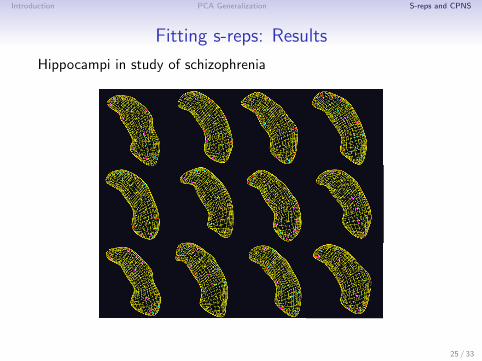
Fitting s-reps: Results
Hippocampi in study of schizophrenia
25 / 33
Introduction PCA Generalization S-reps and CPNS
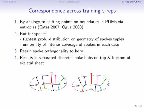
Correspondence across training s-reps
1. By analogy to shifting points on boundaries in PDMs viaentropies (Cates 2007, Oguz 2008)
2. But for spokes:- tightest prob. distribution on geometry of spokes tuples- uniformity of interior coverage of spokes in each case
3. Retain spoke orthogonality to bdry
4. Results in separated discrete spoke hubs on top & bottom ofskeletal sheet
26 / 33
Introduction PCA Generalization S-reps and CPNS
Abstract space of discrete s-reps with n spokes
• Each spoke direction ∈ S2
• log (spoke length) ∈ Rn
• After centering and scaling of tuple of p(u) values,
• These points are in R× S3(n−1)−1 (same as for the PDMs)
The s-rep is a point ∈ Rn+1 × (S2)n × S2(n−1)−1
Composite Principal Nested Sphere is applied
Separately analyze each sphere into Euclideanized variables and,Composite with Euclidean variable to take correlation into account.
27 / 33

Introduction PCA Generalization S-reps and CPNS
Transformations of S-reps
For global rotation
• Each spoke direction moves on a small circle on S2;
• the circles share a common axis
• Scaled tuple of spoke tails move on a small circle (1D sphere)on S3n−4
For rotational fold and twists about an axis
• All spoke directions move on small circles on S2
• The circles share a common axis
Experimentally, analysis via small sphere motions is useful
28 / 33

Introduction PCA Generalization S-reps and CPNS
Shape Probabilities via CPNS
• Successive dimension reduction for spherical variables
• Composite scores from each sphere with Euclidean part, thenSVD
• Yields fewer eigenmodes to explain variation
29 / 33

Introduction PCA Generalization S-reps and CPNS
Shape Probabilities via CPNSModes of variation by principal arcs:
rotation, pinching / elongation, swelling / twisting, swelling in the bottom 30 / 33
Introduction PCA Generalization S-reps and CPNS
Summary
• Backward PCA approaches on spheres and composite spacewith Euclidean space
• Shown useful for 2D, 3D landmark data (PDM)
• S-reps provide a basis for statistics on objects
• In the size and shape changes of hipposcampi s-reps,composite PNS yields succinct description of data
31 / 33

Introduction PCA Generalization S-reps and CPNS
• Cates, J; PT Fletcher, M Styner, ME Shenton, RT Whitaker (2007).Shape modeling and analysis with entropy-based particle systems. Proc.Information Processing in Medical Imaging, Springer LNCS 4584:333-345.
• Damon, J (2003). Smoothness and geometry of boundaries associated toskeletal structures I: sufficient conditions for smoothness, Annales Inst.Fourier 53: 1001-1045.
• Damon, J (2008). Swept regions and surfaces: modeling and volumetricproperties, Conf. Computational Alg. Geom. 2006, in honor of AndreGalligo, Special Issue of Theor. Comp. Science, 392(1-3): 66-91.
• Fletcher, PT; C Lu, SM Pizer, S Joshi (2004). Principal geodesic analysisfor the study of nonlinear statistics of shape, IEEE Transactions onMedical Imaging, IPMI 2003 special issue, 23(8): 995-1005.
• Huckemann, S; H Ziezold (2006). Principal component analysis forRiemannian manifolds with an application to triangular shape spaces.AAPS 38(2): 299-319.
• Huckemann, S; T Hotz, A Munk (2010). Intrinsic shape analysis:geodesic principal component analysis for Riemannian manifolds moduloLie group actions. Statistica Sinica 20(1):1-100.
• Jung, S; I Dryden, D Marron (2011). Analysis of principal nested spheres.Submitted.
32 / 33

Introduction PCA Generalization S-reps and CPNS
• Oguz, I; J Cates, T Fletcher, R Whitaker, D Cool, S Aylward, M Styner(2008). Entropy-based particle systems and local features for corticalcorrespondence optimization. Proc ISBI 2008: 637 – 1640.
• K Siddiqi, Pizer, SM (2008). Medial Representations: Mathematics,Algorithms and Applications, Springer.
• Schulz, J; S Jung, S Huckemann (2011): a collection of internal reportssubmitted to UNC-Gottingen study group on s-rep change underrotational transformations.
33 / 33