NASA Technical Memorandum 108807 lim_F,,L COHTAIHS

I_ ILLU_TUTIO!_

Backward-Facing StepMeasurements at LowReynolds Number, Reh=5000

Srba Jovic, Eloret Institute, Palo Alto, CaliforniaDavid M. Driver, Ames Research Center, Moffett Field, California

February 1994

National Aeronautics andSpace Administration

Ames Research CenterMoffett Field, California 94035-1000

https://ntrs.nasa.gov/search.jsp?R=19940028784 2018-06-03T03:06:46+00:00Z

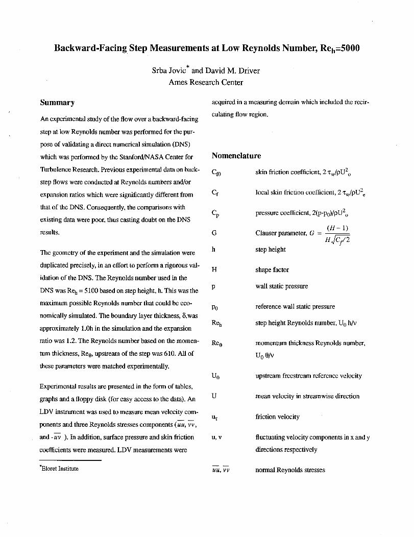
Backward-Facing Step Measurements at Low Reynolds Number, Reh=5000

Srba Jovic* and David M. Driver

Ames Research Center

Summary

An experimental study of the flow over a backward-facing

step at low Reynolds number was performed for the pur-

pose of validating a direct numerical simulation (DNS)

which was performed by the Stanford/NASA Center for

Turbulence Research. Previous experimental data on back-

step flows were conducted at Reynolds numbers and/or

expansion ratios which were significantly different from

that of the DNS. Consequently, the comparisons with

existing data were poor, thus casting doubt on the DNS

results.

The geometry of the experiment and the simulation were

duplicated precisely, in an effort to perform a rigorous val-

idation of the DNS. The Reynolds number used in the

DNS was Reh = 5100 based on step height, h. This was the

maximum possible Reynolds number that could be eco-

nomically simulated. The boundary layer thickness, 5,was

approximately 1.0h in the simulation and the expansion

ratio was 1.2. The Reynolds number based on the momen-

tum thickness, Re0, upstream of the step was 610. All of

these parameters were matched experimentally.

Experimental results are presented in the form of tables,

graphs and a floppy disk (for easy access to the data). An

LDV instntment was used to measure mean velocity com-

ponents and three Reynolds stresses components (uu, vv,

and -uv ). In addition, surface pressure and skin friction

coefficients were measured. LDV measurements were

*Eloret Institute

acquired in a measuring domain which included the recir-

culating flow region.

Nomenclature

Cfo

Cf

%

G

h

H

P

P0

Reh

Re0

u0

U

th

U, V

UU, VV

skin friction coefficient, 2 Xw/pU2o

local skin friction coefficient, 2 _w/pU2e

pressure coefficient, 2(p-p0)/PU2o

Clauser parameter, G -

step height

shape factor

wall static pressure

(H- 1)

reference wall static pressure

step height Reynolds number, U0 h/v

momentum thickness Reynolds number,

U 0 0/v

upstream freestream reference velocity

mean velocity in streamwise direction

friction velocity

fluctuating velocity components in x and y

directions respectively

normal Reynolds stresses

--UV Reynolds shear stress

X r

X, y

mean reattachment length

coordinate system representing stream-

wise and wall-perpendicular directions

measured from the step and the wall

respectively

y+ normalized distance from the wall, yu_/v

V molecular kinematic viscosity of air, nom-

inally 1.5*10Sm2/s at T = 20°C

air density, 1.2 kg/m 3 at T = 20°C

boundary layer thickness where

U = 0.99U e

displacement thickness

0 momentum thickness

"cw wall shear stress

Introduction

The present experimental effort was motivated by a coop-

erative project on complex flows between the Modeling

and Experimental Validation Branch of NASA Ames and

the Stanford]NASA Ames Center for Turbulence

Research. A Direct Numerical Simulation (DNS) of a

backward-facing step configuration was chosen as the sim-

plest geometry to generate a flow with separation that is

equally suitable for experiments and computations (Le,

Moin and Kim (1993a,b)). Reynolds number of the DNS is

limited by the available computer memory and speed to

resolve all time and length scales of turbulence. Thus, the

DNS predictions were confined to a low step height Rey-

nolds number, Re h, of nominally 5000, for which there

were no experimental data to compare. Consequently, an

experiment was devised to match the conditions of the

DNS. The experiment was carried out in a wind tunnel

with a double-sided symmetrical sudden expansion to sim-

ulate the DNS single-sided expansion with a slip condition

on the upper boundary of the computational domain.

The flow field of a separated flow is divided into four

zones which are mutually interrelated. The zones are: the

separated shear layer, the recirculating region under the

shear layer, the reattachment region, and the attached/

recovery region. Each flow region beares some resem-

blance to flows such as mixing layers and boundary layers.

For the most part, the internal shear layer, which develops

within the original boundary layer downstream of the step,

appears to be similar to that of a plane mixing layer.

The objective of the present report is to present measure-

ments of mean velocity, U, and Reynolds stress compo-

nents, uu, vv, and - uv of the flow behind a backward-

facing step for the purpose of rigorously validating the

recent DNS computations of the same flow.

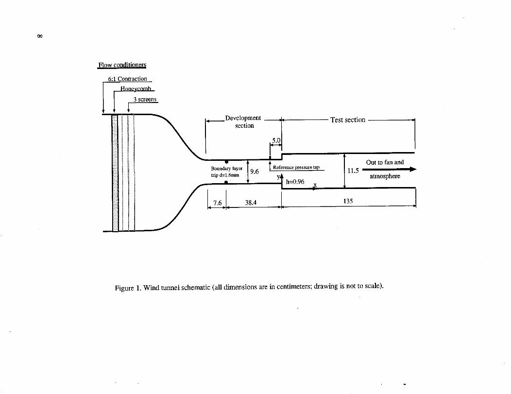
Wind Tunnel and Experimental Techniques

The experiment was conducted in a suction-driven open-

return wind tunnel in the Modeling and Experimental Val-

idation Branch of NASA Ames Research Center. The

wind tunnel is shown schematically in Figure 1. Flow

enters through a settling chamber containing a honeycomb

and a set of three fine screens used for the flow condition-

ing. Flow continues through the two-dimensional 6:1 con-

traction before entering the developing Section. The

boundary layer develops on the walls of a 9.6 cm high by

30.5 cm wide by 46 cm long zero-pressure-gradient duct

before passing into a sudden double-sided expansion. The

tunnel expands symmetrically at the location of the step.

The step height, h, on each side of the tunnel was nomi-

nally0.98cmwhichresultsinexpansionratio,Evof 1.2.

Thetunnelsidewallswereslightlydivergedtocompen-

satefortheblockageeffectduetoboundarylayergrowth.

Thewalldivergencewassettocreateazero-pressure-gra-

dientinboththeupstreamportionofthetunnelwherethe

boundarylayerdevelopsaswellastheregiondownstreamofreattachment.Measurementsweremadeatareference

flowspeed,U0,of7.72m/smeasuredatastation3.0cm

upstreamofthestep.A freestreamturbulenceintensitywaslessthan1%.

Aboundarylayertripwire(1.6mmdia),wasplacedonall

fourwallsofthewindtunnel(at7.6cmdownstreamofthe

entrancetothetest-section)toensurethattheboundary

layerwastransitionedtoturbulenceuniformlyalongthe

span.Theresultingboundarylayerthicknesswas1.15cm

(or1.2h)atx=-3.05hupstreamofthestep.Thiswassuffi-

cientlyclosetothevalueof 1.0hobtainedin thesimula-

tion.TheReynoldsnumber,Re0,basedonthemomentum

thicknesswasnominally610inboththesimulationand

theexperiment.Theintegralparametersfortheboundary

layeratthislocationindicatethattheboundarylayer

closelyresemblesthatofastandard,fullydevelopedzero-

pressure-gradientturbulentboundarylayer.

Table 1. Integral parameters and skin frictioncoefficient at x/h = -3.05

_i(cm) _5*(cm) 0(cm) H 103*Cf

1.15 0.17 0.12 1.45 4.9

Table 2. Maximum values of characteristic turbulent

quantities at x/h=-3.05

-- 2U rms/ Ux V rms/ Ux --UV / Ux R uv

2.90 0.82 0.811 0.51

Values of the integral parameters are shown in Table 1.

The maximum values of uu, vv,-uv, and Ruv for the

upstream location are shown in Table 2. The characteristic

maximum values of the measured Reynolds stresses indi-

cate that the boundary layer is slightly overstimulated by

the tripping device (Erm and Joubert (1991)). No attempt

was made to correct this. The aspect ratio (tunnel width/

step height) of 31 is much greater than the value of 10 rec-

ommended by de Brederode snd Bradshaw (1972) as the

minimum to assure two-dimensionality of a separated

flow.

Instrumentation

Surface static pressures were measured on the upper and

the lower (step-side) walls using a 10 Torr (1300 N/m 2)

Barocel Transducer.

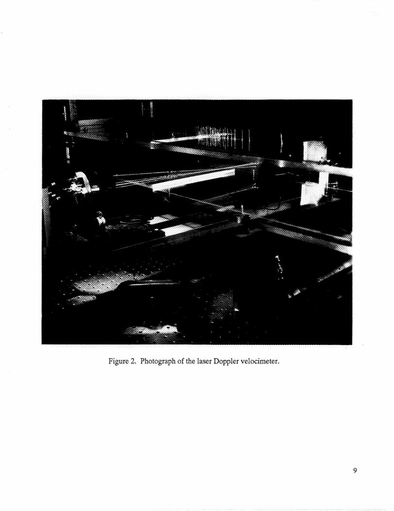
Mean and fluctuating velocities were measured with a

dual-beam, two-component, fiber-optic laser Doppler

velocimeter (LDV), which uses blue and green light (}_ =

488 nm and 514.5 nm) from an argon ion laser for the ver-

tical and streamwise components of velocity, respectively

(see fig. 2). The fringes formed at the intersection of the

blue beam pair (vertical component) were spaced 7.37 txm

apart and the green fringes were spaced 35 _tm. Each

velocity component had one of its two beams bragg shifted

by 40 MHz so as to create a bias in the frequency of the

measured signal, thus allowing the instrument to distin-

guish the direction that the particle is traveling as well as

the speed. Each of the four beams were intersected at a

point inside the wind tunnel (known as the scattering vol-

ume) which measured 0.15 mm in diameter and 1 mm in

length. Tiny (1 lxm) water droplets (suspended in the air

flow) scattered laser light as they passed through the scat-

tering volume. The scattered light was collected by a lens

which focused the light into a fiber through which it trav-

eled to a dichroic light filter that spatially separated the

green laser light from the blue before passing into their

respective photomultiplier tubes. The electrical signals

werethenfilteredandprocessedineachoftwoTSI

counters(model1990).Onlythosesignalsthatarrived

simultaneously(_ 10lxs) were accepted and recorded by

the computer. Those validated velocity pairs were ensem-

ble averaged to obtain statistical measure of U, V, uu, vv,

and -uv. After considering the systematic and random

errors as well as repeatability of measurements it was esti-

mated that mean velocities were measured with + 2%

accuracy and the Reynolds stresses were measured with

+15% accuracy.

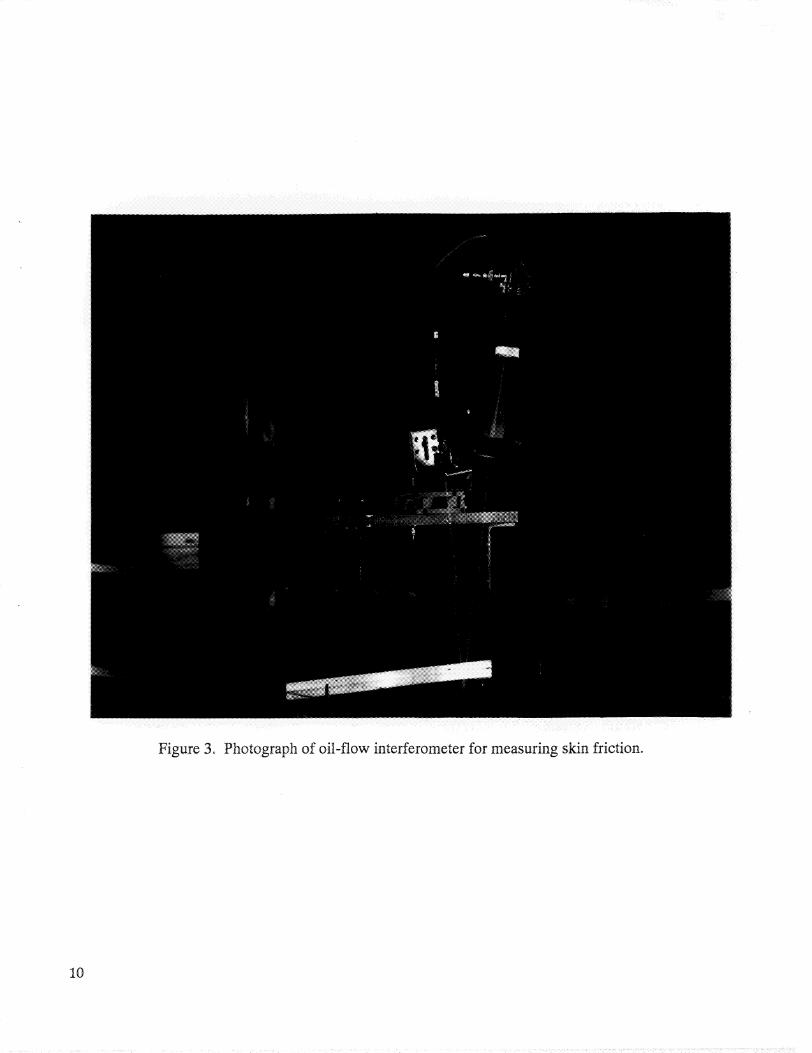
An Oil-Flow Laser Interferometer is used to make direct

measurements of skin friction (see fig. 3). In this tech-

nique, a patch of oil which is placed on the wind tunnel

floor will flow due to surface shear and a laser interferom-

eter is used to measure the thickness of this patch of oil as

a function of time. The interferometer senses the incident

laser light which is reflecting from the air-oil interface as

well as from the metal surface (light reflecting from the

surface passes through the oil) as shown in figure 4. The

two reflecting beams are received at a photodiode where

either constructive or distractive interference takes place

depending on the path length of the light which passes

through the oil. The sinusoidal-like signal produced by the

photodiode is used to determine the change in thickness of

the oil as a function of time, from which the magnitude of

the surface shear (acting on the oil) was determined using

hydraulic theory. Skin friction was measured on the step-

side wall with an uncertainty in the skin friction coefficient

of less than +0.0005 (based on an estimate of the system-

atic errors as well as repeatability). More detailed descrip-

tion of the method Can be found in Monson, Driver and

Szodruch (1981) and Monson and Higuchi (1981).

Results

Surface Pressure Distributions

The wall static-pressure coefficient is defined as

2 (p - Po)

Ct' - P U2o

where p is the wall static pressure at any x location and Po

is the reference wall static pressure measured at xo/h=-5.1

upstream of the step. The pressure-coefficient distribution

measured in the plane of symmetry along the bottom and

top walls are shown in figure 5. Most of the pressure

recovery occurs within 10h of the step. Symmetry of the

pressure distribution along the two walls demonstrates that

the flow was symmetrical with approximately equal reat-

tachment lengths on top and bottom walls.

Pressure-coefficient measurements are presented in tables

3 and4.

Skin Friction Distributions

The skin-friction coefficient, Cf, shown in figure 6, is

defined as

2'_W

ci0- pUo

where pU2o/2 is the reference dynamic head upstream of

the step. Scatter of the data shows the error band of the

experimental technique. Local skin-friction coefficients

were used for normalization of the mean velocity and mea-

sured Reynolds stresses on wall variables in the recovery

region of the flow. The large minimum Value of the skin-

friction coefficient of about -0.003 occurs about 0.67X r

downstream of the step in the recirculating region. This

value is about three times larger than the minimum Cf

measured for high Reynolds number of Driver and Seeg-

miller (1985), Westphal et al. (1984), and Adams et al.

4

(1984).JovicandDriver(tobepublished)experimentally

examinedtherelationshipbetweenminimumCfandReh

and found that the minimum skin friction-coefficient is a

strong function of Re h, increasing sharply for lower Rey-

nolds numbers.

The reattachment length is deduced in two independent

ways and was found to be Xr/h = 6+0.15. The mean

reattachment length was determined from the oil flow

visualization using a low viscosity oil. A second approach

involving an interpolation of the measured skin-friction

coefficient to find the point where Cf = 0. The reattach-

ment length obtained by DNS is 6.0h based on the zero-

crossing of their Cf distribution.

Mean velocity

Flow field velocities and Reynolds stresses of the evolving

turbulent separated flow were measured at six streamwise

locations. Mean velocity is shown in figure 7 in global

coordinates (U/U o vs. y/h) and in Figure 8 in wall coordi-

nates. The first location at x/h = -3.05 was chosen to estab-

lish the state of the incoming low-Reynolds number

turbulent boundary layer. The Reynolds number based on

the momentum thickness at this location was Re = 610.

The location, x/h = 4.0, is approximately the location

where the minimum Cf and the maximum Reynolds

stresses occur. The x/h = 6.0 location is where flow

attaches in a time-average sense, while stations, x/h = 10,

15 and 19, were in the recovery region of the flow.

Mean velocity scaled with inner-wall variables (fig. 8)

suggests that the reattached boundary layer is far from

equilibrium. Deviations of the mean velocity from the

law-of-the-wall were observed by Driver (1991) for a tur-

bulent boundary layer prior to separation due to an adverse

pressure gradient and by Jovic (to be published as NASA

TM) for a recovering boundary layer downstream of a

backward-facing step for different Reynolds numbers. The

flow at reattachment and for some distance downstream

resembles that of the mixing layer (emanating from the lip

of the step) and does not develop with much near-wall

similarity over this region. It appears that the remnants of

the turbulent mixing layer dominate the entire boundary

layer in the vicinity of reattachment and for some distance

downstream. The wall appears to influence only a thin vis-

cous region very near to the wall. Chandrsuda and Brad-

shaw (1981) and Jovic (1993), analyzing the balance of

turbulent kinetic energy, showed that the recovering flow

downstream of the mean reattachment point is far from

equilibrium (production of turbulent kinetic energy is not

equal to the rate of dissipation).

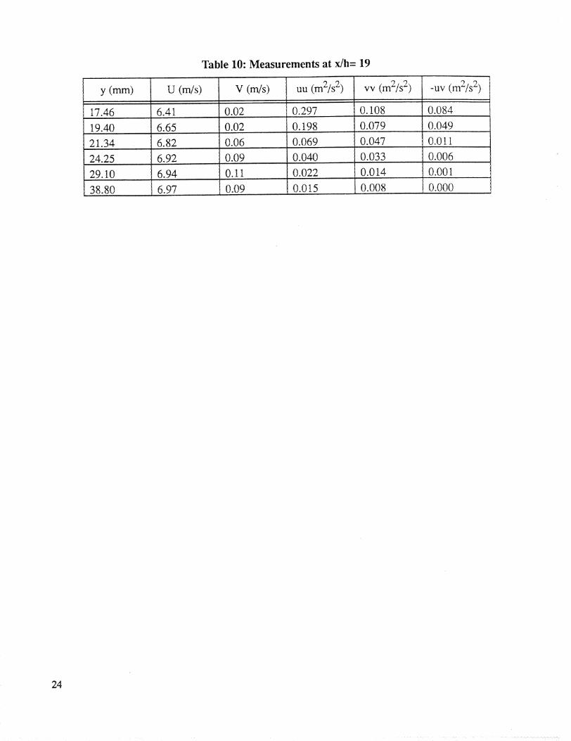
Measured mean velocity and the Reynolds stress data are

listed in tables 5 through 10 of the Appendix.

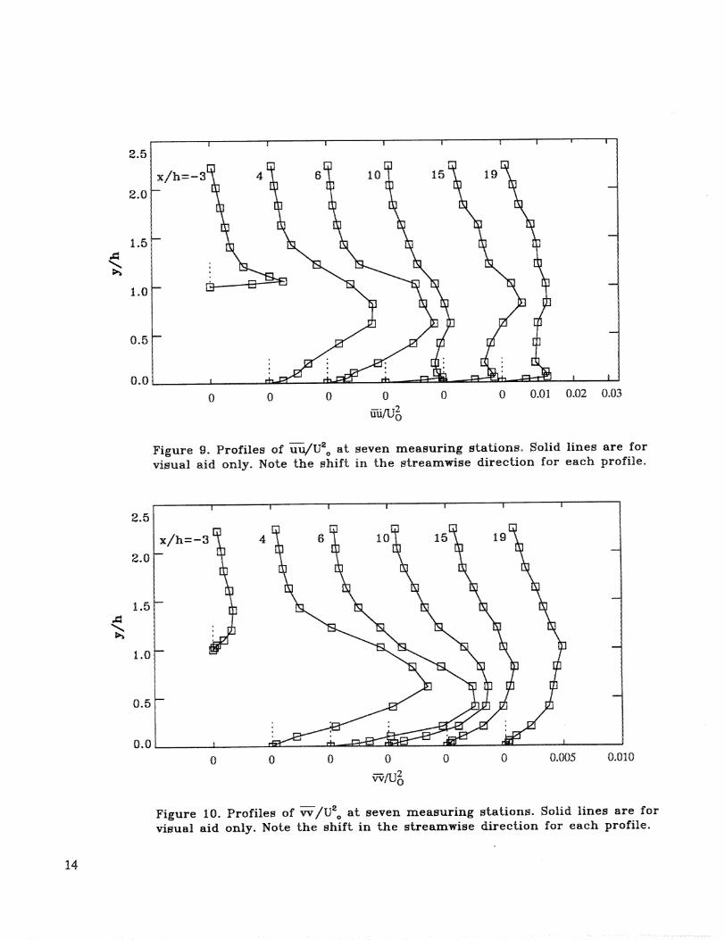
Reynolds stresses

Profiles of Reynolds-stresses, u u, vv, and - uv normalized

by U2o are shown in Figures 9, 10 and 11 respectively. All

turbulent Reynolds stresses increase rapidly from the point

of separation until about 0.67X r where they reach a maxi-

mum. This rapid growth resembles that of the near field of

a free shear layer. Beyond this point turbulence activity

decays and gradually approaches the stress levels seen in

an equilibrium boundary layer.

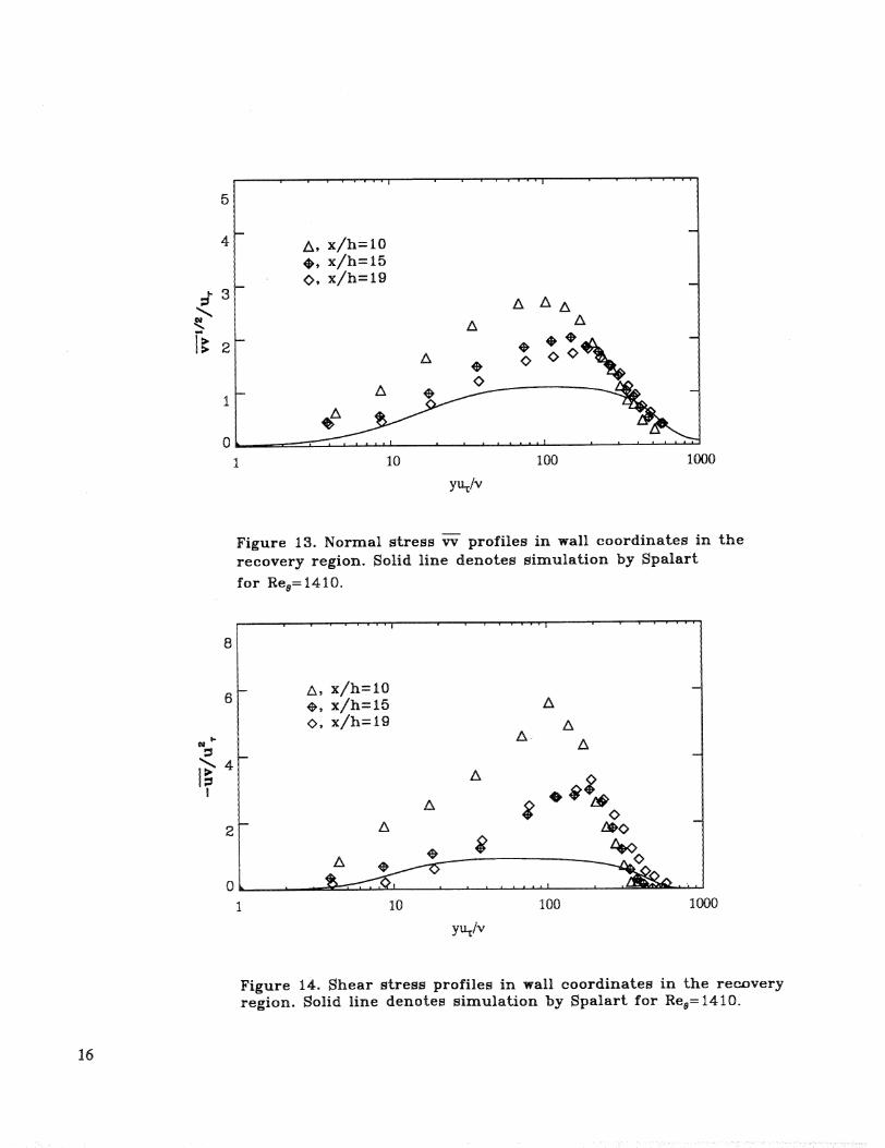
In the recovery region, Reynolds stresses normalized with

wall coordinates, using the local Cf are shown in figures

12 through 14. The Reynolds stresses in the inner layer

recover to levels comparable to that of an ordinary turbu-

lent boundary layer (simulated by Spalart (1988)) by the

time the flow reaches the x/h = 19 station. However, in the

outer layer the Reynolds stresses decay much more slowly,

owing to the persistence of large eddies which were gener-

atedin theshearlayerupstream.Thesestressesintheouterregionpersistathighlevelsuntilquitefardown-

stream(probably100h),unlikethestressesin theinner

regionoftheflowwhichconvergetoanequilibriumlevel

within25hto30hofthestepaccordingtoJovic(1993).

Concluding remarks

A joint effort between the Modeling and Experimental

Validation Branch of NASA Ames and Stanford/NASA

Ames Center for Turbulence Research was conducted to

understand the flow physics of the separating and reattach-

ing turbulent boundary layer behind a backward-facing

step.

Backward facing step flows are sensitive to step height

Reynolds number, Re h, (Jovic, to be published as a NASA

TM), expansion ratio, and _/h making it necessary to per-

form another backward-facing step flow experiment which

closely duplicated the DNS conditions.

In the recovery region of the flow, the log-law of the mean

velocity is not obeyed and does not exist as has been seen

in previous sets of data (Driver-Seegmiller). This was also

seen in Jovic (to be published as a NASA TM) for a num-

ber of different Reynolds numbers and levels of perturba-

tion.

The results of this experiment show that the flow structure

at this low Reynolds number is qualitatively similar to

structures of flows at much higher Reynolds numbers.

However, the magnitudes of turbulent quantities are

dependent primarily on the Reynolds number, Re h, and

the strength of perturbation expressed by 5/h.

References

1. Adams, E.W., Johnston, J.P. and Eaton, J.K.: Experi-

ments on the structure of turbulent reattaching flow.

Report MD-43, Department of Mechanical Engineering,

Stanford University, 1984.

2. Chandrsuda, C. and Bradshaw, E: Turbulence structure

of a reattaching mixing layer. J. Fluid Mech. 110, 1981,

pp.171-194.

3. Driver, D.M. and Seegmiller, H.L.: Features of a reat-

taching turbulent shear layer in divergent channel flow,

AIAA J. 23, 1985, p.163.

4. Driver, D.M.: Reynolds shear stress measurements in a

separated boundary layer flow. AIAA Paper 91-1787,

Honolulu Hawaii Meeting, 24-27 June, 1991.

5. deBredorod, V. and Bradshaw, P.: Three-dimensional

flow in nominally two-dimensional separation bubbles.

Flow behind a rearward-facing step. I.C. Aero Report

72-19.13, 1972.

6. Erm,L.P. and Joubert, EN.: Low-Reynolds number tur-

bulent boundary layer. J. Fluid Mech., 230, 1991, pp.l-44.

7. Jovic, S.: An experimental study on the recovery of a

turbulent boundary layer downstream of the reattachment.

Proceedings of the Second International Symposium on

Engineering Turbulence Modelling and Measurements,

Florence, Italy, 31 May-2 June, 1993.

8. Le, H., Moin, P. and Kim, J.: Direct numerical simula-

tion of turbulent flow over a backward-facing step. Report

TF-58, Thermosciences Division, Department of Mechan-

ical Engineering, Stanford University, 1993.

9. Le, H., Moin, P. and Kim, J." Direct numerical simula-

tion of turbulent flow over a backward-facing step. 9th

Symposium on Turbulent Shear Flows, Tokyo, 1993.

10. Monson, D., Driver, M.D. and Szodruch, J.: Applica-

tionofaLaserInterferometerskin-frictionmeterincom-

plexflows.ICIASF'81Record,Internationalcongresson

InstrumentationinAerospaceSimulationFacilities,1981,

ppo232-243.

11.Monson,d.andHaguchi,H.: SkinFrictionmeasure-

mentsbyadual-laser-beaminterferometertechnique,

AIAAJ.19,1981,p.739.

12.Spalart,ER.: Direct simulation of a turbulent boundary

layer up to Re=1410. J. Fluid Mech. 187, 1988, pp.61-98.

13. Westphal, R.V., Johnston, J.P. and Eaton, J.K.: Experi-

mental study of flow reattachment in a single-sided sudden

expansion. Report MD-41, Department of Mechanical

Engineering, Stanford University, 1984.

oo

Flow cgnditioners

6:1 Contraction

l [ Honeycomb3 screens

7.6

Development J.

section 5_.O.-

a I

Boundary layer 9.6 l pressure tap

trip d=l.6mm

A

Test section

11.5

Y_ h=0.96

38.4 .[ 135r_

Out to fan and

atmosphere

Figure 1. Wind tunnel schematic (all dimensions are in centimeters; drawing is not to scale).

........ i;i i....... _ i i; i ii i iiii iii_ i ii i_ iii i ii iii!iiiiiiiiiiii_iii ¸iiii i _ ?

Figure 3, Photograph of oil-flow interferometer for measuring skin friction,

10

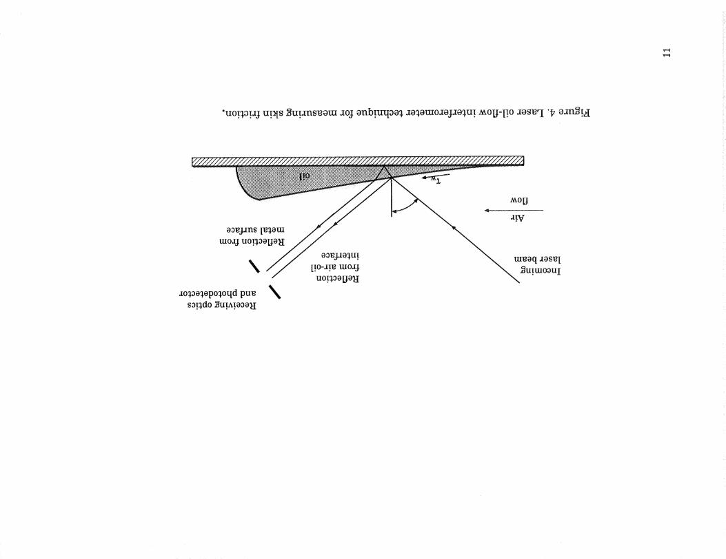
"uot._,ot,2jut._[s_ut.2ns_om2ojonbt.uqoo_,2o_,otuo2oj2o_,ut.A_ou-[t.o2os_I "17o.m_t.al

v_

v_

0.30

0.20

r.) 0.I0

0.00

-0.10

-5

| B i 1

m

_ n Bottom wall -

A Top wall

0 5 10 15 20

x/h

Figure 5. Distribution of pressure coefficient along top and bottom walls

downstream of the step. Solid line represents pressure distribution obtained

by the simulation.

0.004

0.002

0.000

-0.002

-0.004

| | i

D

0 5 10

Z]

Z]

I

15 20

x/h

Figure 6. Distribution of skin-friction coefficient in the streamwise direction.

Solid line represents skin-friction coefficient obtained by the simuldtion.

12

1.5

1.O

35

3O

25

2O

15

10

| | | | i | |

0 0 0 0 0 0 0 1.0

U/Uo

Figure 7, Profiles of mean streamwise velocity profiles for seven measuringstationS. Solid lines are for visual aid only. Note the shift in the streamwise

direction for each profile.

........ i ........ |

n, x/h=-3

A, x/h=10_, x/h= 15O' x/h=19

1 10

_A _

nD--

JO

m_

100 1000

Figure 8. Mean velocity profiles in wall coordinates in the recovery region.Solid line represent standard liner and log relationships in the inner layer.

13

1.5

1.0

0.5

| I | | | | | g

x/h=-3 6 1O 5B

m

0 0 0 0

_-LVU20

t

t

0 0 0.01 0.02 0.03

Figure 9. Profiles of u--u/UZo at seven measuring stations° Solid lines are for

visual aid only. Note the shift in the sLreamwise direction for each profile.

14

1.5

1.0

| | | ! | g |

0 0 0 0 0 0.005 0.010

Figure 10. Profiles of _/U2o at seven measuring stations. Solid lines are for

visual aid only. Note the shift in the streamwise direction for each profile.

1.5

1.0

I

0

J | 0 i i |

4 6 10 15 19

j m

0 0 0 0 0 0 0.005 0.010

Figure 11. Profiles of-uv/UZo at seven measuring stations. Solid lines

are for visual aid only. Note the shift in the sLreamwise direction for

each profile.

. s • = . _ • . | . ' ' _ ' • ' ' |

ZX, x/h-lO@, x/h= 15

O, x/h=19A A @

A A @ A

g g . ° oaO._ -

%

1 10 100 1000

Figure 12. Normal stress u--uprofiles in wall coordinates in the recovery

region. Solid line denotes simulation by Spalart for Re e=1410.

15

N

........ | ........ D

A, x/h= 10@, x/h= 15<>, x/h= 19

A

A A AA

<>A @

• . = . i . n

I 1() lO0 1000

Figure 13. Normal stress vv profiles in wall coordinates in the

recovery region. Solid line denotes simulation by Spalart

for Ree= 1410.

N

1 4I

........ | ........ i

A, x/h- 10e, x/h- 15O, x/h- 19

A

A

A

<>

h,.

1 10 100 1000

y%/v

Figure 14. Shear stress profiles in wall coordinates in the recoveryregion. Solid line denotes simulation by Spalart for Ree=1419.

16

Appendix

Uo=7.72m/s h=0.98cm Reh= 5000 xr/h= 6.0

Reference wall static pressure is measured in x/h=-5.1

Reference velocity U o is measured in x/h=-3.05

Table 1: Integral parameters

Ue(m/s) 0(mm) g(mm) H Re 0 103"Cf G

-3.05 7.72 1.73 1.19 11.5 1.45 610 4.90 6.24

4.0 7.41 10.47 1.96 5.33 970 -2.72 N/A

6.0 7.12 8.41 2.98 2.82 1416 0.00 N/A

10.0 6.97 6.53 3.46 1.89 1608 2.35 13.71

15.0 6.75 5.95 3.52 1.69 1585 2.83 10.85

22.0

21.0

22,5

24.0

24.05.80 1.636.95 16513.56 3.0019.0 9.97

Table2: Cf measurements

3.33

3.50

3.58

4.17

5.17

7.08

7.08

8.00

8.50

10.0

Cfx/h

-0.00207

-0.00336

-0.00321

-0.00268

-0.00218

-0.00103

0.00113

0.0015O

0.00154

0.00237

17

E

c_

. ! e • o . , . e

..................................................................!...........................L..... ]...........................

c_

c_

N

E

_D

e_

rJ_

M

I

|

J

o,o o",,i k,"<_ L"-'-

0 QIO 0I ! i I

. . . e

...................

c_r .,_1 _r"_

r--.

oI

O0

c_

0c)

C:) c_ ('--.• C_ C_

i C_ Q

C_0 t ,

0

0 u_

<:_ v">l 0• . | e

oo 0'_ r--- _ _i "_

_ _ _ _i q",l

..... _ _ ........ _=.._ ............

t¢_ 0 u'3 ¢2) u'31 Qo o o ® . _

_ t'-- t_ c_ _1 _,,

Table 3" Pressure coefficient along the bottom wall of the tunnel

2O

21

22

23

24

25

26

27

28

3O

x/h

9.5

I0.0

10.5

11.0

12.0

14.0

16.0

20.0

24.0

28.0

32.0

Cp0.2053

_

0.2053

0.2103

0.2087

0.2091

0.2160

0.2148

0.2118

0.2148

0.2160

0.2160

Table 4: Pressurre coefficient along the top wall of the tunnel

#pt

1

3

4

7

9

11

12

13

14

15

16

0.083

0.333

O.875

1.375

1.875

2.375

3.000

3.500

4.000

4.500

5.333

5.917

6.333

6.833

7.333

7.750

Cp

-0.0335,_

-0.0323

-0.0354

-0.0346

-0.0426

-0.0464

-0.0380

-0.0057

0.0312

0.0722

O. 1217

0.1445

O. 1635

0.1749

0.1863

O. 1932

19

Table 4" Pressurre coefficient along the top wall of the tunnel

17

18

19

2O

21

22

23

24

25

26

27

28

#pt x/h

8.333

8.917

9.833

10.75

11.25

12.00

13.33

14.667

16.00

18.667

21.333

32.00

Cp

0.1977

0.2110

0.2065

0.2095

0.2114

0.2137

0.2122

0.2152

0.2148

0.2148

0.2179

0.2186

Table 5: Measurements at x/h= -3.12

y (mm) U (m/s)

0.25 1.91

0.49

0.97

1.94

3.88

5.82

3.49

4.83

5.61

6.36

6.79

7.76 7.24

9.70 7.46

tl.64 7.66

13.58 7.71

15.52 7.72

17.46

19.40

21.34

24.25

29.10

28.80

7.71

7.69

7.68

7.68

7.71

7.70

v (m/s)

0.00

0.00

-0.01

0.00

0.01

0.04

uu (m2/s 2)

0.711

1.232

1.003

0.563

0.341

0.260

0.04 O. 179

0.08 0.105

0.07 0.031,,

0.06

0.06

0.04

0.03

0.04, ,

0.06

O.02

-0.01

0.011

0.008

0.007

0.012

0.012

0.006

0.006

0.007

I vv (m2/s 2)

0.008

0.019

0.055

0.093

0.101

0.083

0.056

0.044

0.024

0.013

0.010

0.010

0.010

0.009

0.008

0.009

O.O08

-uv (m2/s 2)

0.027

0.078n

0.115

0.106

0.096

0.070

0.042

0.022

0.006

0.000

-0.001

-0.001

0.000.....

-0.001

0.000

0.000

0.000

2O

Table 6: Measurementsat x/h= 4

y(mm)

0.25

O.97

1.94,,

3.88

5.82

7.76

9.70

U (m/s)

-0.59

-1.06

-0.92

-0.18

1.02

2.60

4.00

11.64 5.19

13.58 6.03

15.52 6.50

17.46 6.84

19.40

21.34

24.25

29.10

i 28.80

7.07

7.27

7.38

7.36

7.41

v (m/s)

0.02

-0.04

-0.09

-0.22

-0.43

-0.49

-0.51

-O.44

-0.39

-0.36

-0.32

-0.29

-0.25

-0.21

-0.16

-0.09

uu (m2/s 2)

0.236

0.48 I

0.658

vv (m2/s 2)

0.019

0.124

0.323

1.189 0.615

1.755 0.794

1.766 0.717

1.389 0.556

0.820 0.306

0.387 O. 144

0.221 0.089

0.171

0.102

0.053

0.017

0.011

0.009

0.059

0.042

0.026

0.01I

0.007

-uv (m2/s 2),,

-0.001

0.041

0.162

0.418

0.620

0.582....

0.433

0.230

0.091

0.053

0.032

0.018

0.007

0.001

0.000

0.001

Table 7: Measurements at x/h= 6

y (ram)

0.25

0.49

0.97

1.94

3.88

5.82

7.76

9.70

11.64

13.58

15.52

17.46

U (m/s)

0.08

0.16

0.26

0.72

1.49

2.55

3.64

4.51

5.40

5.94

6.33

6.65

V (m/s)

-0.08

-0.08

uu (m2/s 2)

0.218

0.356

-0.12 0.452

-0.20 0.862

-0.33 1.464

-0.47

-0.45,,,

-0.39

-0.37

-0,34

-0.31

1.823

1.635

vv (m2/s 2)

0.127

0.199

0.306

-uv (m2/s 2)

0.O5O.... I

0.099

0.I58

0.3770.572

0.737 0.603

0.724 0.647

0.566 0.495

1.511 0.367 0.299

0.556 0.258 O. 195

0.29,6 O. 147 0.092..

0.087

0.050

0.185

0.105

0.047

0.027

21

y (mm)

19.4021.3424.2529.1038.80

U (m/s)

6.83

6.98

7.07

7.1I

7.17

Table 7: Measurements at x/h= 6

v (m/s) uu (m2/s 2)

0.070

0.031

0.012

0.009

0.009

vv (m2/s 2)

0.034

0.024

0.010

0.005

0.OO5

-uv (m2/s 2)

0.014

0.008

0.001

0.001

0.001

y (mm)

0.25

0.49

0.97

1.94

3.88

5.82

7.76

9.70

11.64

13.58

15.52

17.46

t9.40

21.34

24.25

29.t0

38.80

Table 8: Measurements at x/h= 10

U (m/s)

1.07

1.46

2.11

2.52

3.04

3.64

4.24

4.80

5.44

5.89

6.23

6.53

6.74

6.81

6.89

6.96

6.99

V (m/s)

-0.04

-0.08

-0.13

-0.21

-0.26

-0.30

-0.21

-0.21

-0.12

-0.09

-0.06

-0.06

-O.O7

-0.06

-0.10

-0.08

uu (m2/s 2)

0.658

0.968

0.875

0.840

0.939

1.114

1.013

0.850

0.555

0.418

0.287

O. 145

0.088

O.O7O

0.045

0.O2O

0.026

vv (m2/s 2)

0.027

0.076

O. 190

0.356

0.495

0.507

0.471

0.388

0.258

0.189

0.140

0.085

0.049

0.O41

0.0t5

0.006

O.005

-UV (m2/s 2)

0.059

0.132,,,

0.178,,

0.240

0.322

0.392

0.344

0.304

0.183

0.130

0.O95

0.050

0.014

0.015

0.002

0.000

0.000

22

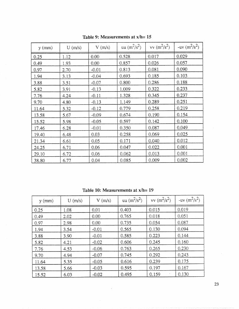
Table 9: Measurementsat x/h= 15

y (ram)

0.25

0.49

U (m/s)

1.12

1.93

0.97 2.70

1.94 3.13

3.88

5.82

7.76

9.70

11.64

13.58

15.52

17.46

19.40

21.34

24.25

29.10

38.80

3.51

3.91

4.24

4.80

5.32

5.67

5.98

6:.28

6.48

6.61

6.71

6.72

6.77

V (m/s) uu (m2/s 2)

0.00 0.528

0.00 O.857

-0.01 0.813

-0.04 0.693

-0.11,,

-0.13

-0.12

-0.09

-O.05

-0.01

0.03

0.05

0.06

0.06

O.O4

0.800

1.009

1.328

1.149

0.779

0.674

0.597

0.350

0.258

0.171

0.047

0.062

0.085

vv (m2/s 2)

0.017

0.026

0.081

0.185

0.286

0.322

0.345

0.289

0.258,,,

0.190

0.142

O.087

0.069

O.O4O

0.022

0.013

0.009

-uv (m2/s 2)

0.029

0.057

0.090

0.i03....

O. 188

0.233

0.237

0.251

0.219

0.154

0.100

0.049

0.025

0.012

0.001

0.001

O.OO2

Table 10: Measurements at x/h= 19

y (mm)

0.25

0.49

0.97

1.94

3.88

5.82

7.76

9.70

t 1.64

13.58

15.52

U (m/s)

1.08

2.02

2.98

3.54

3.90

4.21

4.53

4.94

5.35

5.66

6.03

v (m/s)

0.01

0.00

0.00

-0.07

uu (m2/s 2)

0.403

0.765

0.735

0.565

O.585

0.606

0.763

0.745

vv (m2/s 2)

0.015

0.018

0.054

0.130

0.223

0.245

0.265

0.292

0.616

0.595

0.495

0.2139

0.197

0.159

-uv (m2/s 2)

0.019

I 0.05 t

0.087

0.094

0.144

0.160

0.230

0.243

0.t75

0.167

0 t30

23

y (mm)

17.46

Table 10: Measurements at x/h- 19

U (m/s)

6.41

6.65

V (m/s)

0.02

uu (m2/s 2)

0.297

vv (m2/s 2)

0.108

-uv (m2/s 2)

0.O84

19.40 0.02 O. 198 0.079 0.049

21.34 6.82 0.06 0.069 0.047 0.011

24.25 6.92 0.09 0.040 0.033 0.006

29.10 6.94 O. 11 0.022 0.014 0.001

38.80 6.97 0.09 0.015 0.008 0.000

24

I Form ApprovedREPORT DOCUMENTATION PAGE ouBNoo7o4-o188

Public reporting burden for this collection of information is estimated to average 1 hour per response, including the time for reviewinginstructions,searching existing data sources,gathering and maintaining the data needed, and completing and reviewing the collection of information. Send comments regarding this burden estimate or any other aspect of thiscollection of information,including suggestions for reducing this burden, to Washington Headquarters Services, Directorate for information Operations and Reports, 1215 JeffersonDavis Highway, Suite 1204, Arlington, VA 22202-4302, and to the Office of Management and Budget, Paperwork Reduction Project (0704-0188), Washington, DC 20503.

I" AGENCYUSEONLY(Leaveblank) I2"REPORTDATEFebruary1994 I 3" REPORTTYPEANDDATESCOVEREDTechnicalMemorandum4. TITLE AND SUBTITLE 5. FUNDING NUMBERS

Backward-Facing Step Measurements at Low Reynolds Number,Reh=5000

6. AUTHOR(S)

Srba Jovich and David M. Driver

7. PERFORMING ORGANiZATiON NAME(S) AND ADDRE:SS{ES)

Ames Research Center

Moffett Field, CA 94035-1000

9. SPONSORING/MONITORING AGENCY NAME(S) AND ADDRESS(ES)

National Aeronautics and Space Administration

Washington, DC 20546-0001

505-59-50

:8....PERFORMING ORG;ANIZATiONREPORT NUMBER

A-94043

I 0. SP:ONSORINGIMONITORINGAGENCY REPORT NUMBER

NASA TM-108807

11. SUPPLEMENTARY NOTES

Point of Contact: Srba Jovich, Ames Research Center, MS 229-1, Moffett Field, CA 94035-1000;

(415) 604-6192

12a. DISTRIBUTION/AVAILABIL|TY STATEMENT

Unclassified _ Unlimited

Subject Category 34

12b. DISTRIBUTION CODE

13. ABSTRACT (Maximum 200 words)

An experimental study of the flow over a backward-facing step at low Reynolds number was performed for the purposeof validating a direct numerical simulation (DNS) which was performed by the Stanford/NAS A Center for TurbulenceResearch. Previous experimental data on backstep flows were conducted at Reynolds numbers and/or expansion ratioswhich were significantly different from that of the DNS.

The geometry of the experiment and the simulation were duplicated precisely, in an effort to perform a rigorous vali-dation of the DNS. The Reynolds number used in the DNS was Reh=5100 based on step height, hoThis was the max-imum possible Reynolds number that could be economically simulated. The boundary layer thickness, d,wasapproximately 1.0h in the simulation and the expansion ratio was 1.2. The Reynolds number based on the momentumthickness, Ree, upstream of the step was 610. All of these parameters were matched experimentally.

Experimental results are presented in the form of tables, graphs and a floppy disk (for easy access to the data). An LDVinstrument was used to measure mean velocity components and three Reynolds stresses components. In addition,

surface pressure and skin friction coefficients were measured. LDV measurements were acquired in a measuringdomain which included the recirculating flow region.

14. SUBJECT TERMS

LDV measurements (Laser DopplerVelocimeter), Separated Flows, Backward-

Facing Step, DNS Code Validation (Direct Numerical Simulation)

17" SECURITY CLASSIFICATION 118' SECURITY CLASSIFICATION 119" SECURITY CLASSIFICATIONOFUnc REPORTIassified OFUncTHISlassifiedPAGE OF ABSTRACT

NSN 7540-01-280-5500

15. NUMBER OF PAGES

2:816. PRICE CODE

A03

20. LIMITATION OF ABSTRACT1

lStandard Form 298 (Rev. 2-89)Prescribed by ANSI Std. Z39-18