WORKING PAPER

Backtesting Counterparty Risk: How Good is your Model?

Ignacio Ruiz ∗

July 2012

Version 2.0.1

Abstract

Backtesting Counterparty Credit Risk models is anything but simple. Such back-testing is becoming increasingly important in the financial industry since both theCCR capital charge and CVA management have become even more central to banks.In spite of this, there are no clear guidelines by regulators as to how to perform thisbacktesting. This is in contrast to Market Risk models, where the Basel Committeeset a strict set of rules in 1996 which are widely followed. In this paper, the au-thor explains a quantitative methodology to backtest counterparty risk models. Heexpands the three-color Basel Committee scoring scheme from the Market Risk tothe Counterparty Credit Risk framework. With this methodology, each model canbe assigned a color score for each chosen time horizon. Financial institutions canthen use this framework to assess the need for model enhancements and to managemodel risk.

Since the 2008 financial crisis, the world of banking is changing in a very fundamentalway. One of the main driver of this transformation is the change in stand by governments,from a “loose” regulatory enviroment in the pre-2007 era to a much more hands-onapproach now. In particular,

1. National regulators have substantially increased their scrutiny over the modelsused by banks to calculate risk and capital.

2. The amount of capital that banks need to hold against their balance sheet hasincreased substantially and, hence, the cost-benefit balance of investing in goodaccurate models has shifted substantially towards better models.

The Basel Committee on Banking Supervision states that banks using their internalmodel methods (IMM) for capital requirements must backtest their models on an on-

∗Founding Director, iRuiz Consulting, London. Ignacio is a contractor and independent consultantin quantitative risk analytics and CVA. Prior to this, he was the head strategist for Counterparty Risk,exposure measurement, at Credit Suisse, and Head of Market and Counterparty Risk Methodology forequity at BNP Paribas. Contact: ignacio@iruizconsulting.com

WORKING PAPER

going basis. Here, “backtesting” refers to comparing of the model’s output againstrealized values.

There are two major areas where backtesting applies: in the calculation of the Value atRisk (VaR), that later feeds into the Market Risk capital charge, and in the calculationof EPE1 profiles, that feed into the Counterparty Credit Risk (CCR) and CVA-VaRcharge. The Basel Committee has stated very clear rules as to how to perform the VaRbacktest, as well as to what are the boundaries discriminating good and bad models.The Committee is also clear about the consequences of a negative backtest for financialinstitutions [1].

However, at present, directives by the Basel Committee regarding EPE backtestingare not so strict. In fact, the Basel Committee has only provided guidelines in thisrespect; details are left to the national regulators to decide on [2]. This has createdsome degree of confusion between and within financial institutions, as they face a blendof (sometimes not clear) requirements from a number of national regulators. As a result,in the author’s view, the global financial system is now exposed to regulatory “arbitrage”in this area.

In this paper, we first outline the backtesting framework set for market risk models bythe Basel Committee. Thereafter, we explain the additional difficulties that counterpartyrisk models bring to with regards to the backtesting, and, then, we propose a method-ology for expanding the Basel’s VaR backtesting framework to the context of CCR ina consistent way. This will be provided with a number of examples that illustrate thestrengths and limits of the methodology.

As mentioned, there is a quite limited literature in this topic, especially in the EPEcontext. This paper compiles information in references [1, 2, 3, 4] and elaborates fromit.

Market Risk Backtesting

In 1996, the Basel Committee set up very clear rules regarding backtesting of VaRmodels for IMM institutions [1]. This section highlights a number of key features of thatbacktesting framework.

The VaR capital charge is based on 10-day VaR. However, backtest is done in 1-day VaR.This is because, as stated in reference [1], “significant changes in the portfolio compo-sition relative to the initial positions are common at major trading institutions”. As aresult, “the backtesting framework . . . involves the use of risk measurements calibratedto a one-day holding period”2.

1Expected Positive Exposure: the average of portfolio values when floored at zero, called “EE” bythe Basel Committee.

2However, the Basel Committee expresses concerns that “the overall one-day trading outcome is not

2

WORKING PAPER

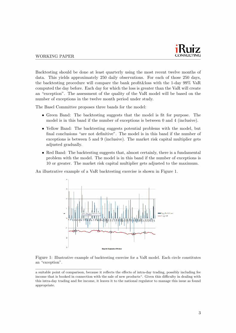
Backtesting should be done at least quarterly using the most recent twelve months ofdata. This yields approximately 250 daily observations. For each of those 250 days,the backtesting procedure will compare the bank profit&loss with the 1-day 99% VaRcomputed the day before. Each day for which the loss is greater than the VaR will createan “exception”. The assessment of the quality of the VaR model will be based on thenumber of exceptions in the twelve month period under study.

The Basel Committee proposes three bands for the model:

• Green Band: The backtesting suggests that the model is fit for purpose. Themodel is in this band if the number of exceptions is between 0 and 4 (inclusive).

• Yellow Band: The backtesting suggests potential problems with the model, butfinal conclusions “are not definitive”. The model is in this band if the number ofexceptions is between 5 and 9 (inclusive). The market risk capital multiplier getsadjusted gradually.

• Red Band: The backtesting suggests that, almost certainly, there is a fundamentalproblem with the model. The model is in this band if the number of exceptions is10 or greater. The market risk capital multiplier gets adjusted to the maximum.

An illustrative example of a VaR backtesting exercise is shown in Figure 1.

Figure 1: Illustrative example of backtesting exercise for a VaR model. Each circle constitutesan “exception”.

a suitable point of comparison, because it reflects the effects of intra-day trading, possibly including feeincome that is booked in connection with the sale of new products“. Given this difficulty in dealing withthis intra-day trading and fee income, it leaves it to the national regulator to manage this issue as foundappropriate.

3

WORKING PAPER

The Probability Equivalent of Colour Bands

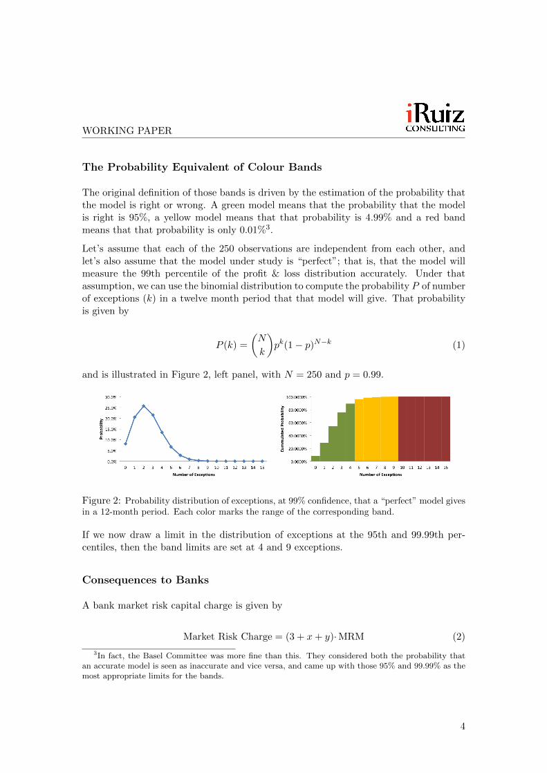
The original definition of those bands is driven by the estimation of the probability thatthe model is right or wrong. A green model means that the probability that the modelis right is 95%, a yellow model means that that probability is 4.99% and a red bandmeans that that probability is only 0.01%3.

Let’s assume that each of the 250 observations are independent from each other, andlet’s also assume that the model under study is “perfect”; that is, that the model willmeasure the 99th percentile of the profit & loss distribution accurately. Under thatassumption, we can use the binomial distribution to compute the probability P of numberof exceptions (k) in a twelve month period that that model will give. That probabilityis given by

P (k) =

(N

k

)pk(1− p)N−k (1)

and is illustrated in Figure 2, left panel, with N = 250 and p = 0.99.

Figure 2: Probability distribution of exceptions, at 99% confidence, that a “perfect” model givesin a 12-month period. Each color marks the range of the corresponding band.

If we now draw a limit in the distribution of exceptions at the 95th and 99.99th per-centiles, then the band limits are set at 4 and 9 exceptions.

Consequences to Banks

A bank market risk capital charge is given by

Market Risk Charge = (3 + x+ y)·MRM (2)

3In fact, the Basel Committee was more fine than this. They considered both the probability thatan accurate model is seen as inaccurate and vice versa, and came up with those 95% and 99.99% as themost appropriate limits for the bands.

4

WORKING PAPER

where x is given by the model performance, y is an add-on that national regulators canimpose at their discretion and the Market Risk Measure (MRM) was 10-day VaR butit is now 10-day-VaR plus stress-10-day-VaR under Basel III. Also, some regulators addan additional component called Risks not in VaR (RniV), which accounts for the marketrisks which are not captured by the VaR model.

Regarding backtesting implications into the capital requirements, x is the number atstake. That number is given by the following table:

Band Num. Exceptions x

Green 0 to 4 0.005 0.406 0.50

Yellow 7 0.658 0.759 0.85

Red 10+ 1.00

After the large number of exceptions that all banks had in the 2008 financial crisis, somenational regulators decided to remove the cap in x and increased it further as the numberof exceptions went beyond 10.

Proposed Framework for Counterparty Risk Backtesting

Regarding counterparty risk models, The Basel Committee has not provided a clearset of rules for backtesting as it has for market risk. Instead, all it has given is aset of guidelines for banks and national regulators [2]. In fact, the Basel Committeestates in that document that “It is not the intention of this paper to prescribe specificmethodologies or statistical tests [for counterparty risk], nor to constrain firms’ abilityto develop their own validation techniques”. As a result, in the author’s experience,backtesting methodologies in banks have become cumbersome, inconsistent and difficultto relate to each other.

The goal of this section is to propose a methodology in the context of counterparty riskthat can be related to the strict backtesting framework which is in place for market risk,that is scientifically sound, practical and that can be easily used by management. Inorder to achieve this, we will

1. Define the context and scope in which backtesting can be done for counterpartyrisk models.

2. Define a single number measure for the quality of a model in a given time horizon.

3. Relate that single number measure to the three bands proposed by the BaselCommittee, allowing one to classify a model to either the green, yellow or red

5

WORKING PAPER

band.

Methodology

Context and Scope

It is general practice to refer to a CCR model backtest as the backtest of the modelsgenerating EPE profiles [2]. Those models can be decomposed into a number of sub-models: Risk Factor Evolution (RFE) models for the stress-testing of the underlyingfactors (e.g., yield curves, FX rates), pricing models for each derivative, collateral modelsfor secured portfolios, and netting and aggregation models.

What we really want is that the value of the whole portfolio under consideration isproperly modelled by the EPE model, which is the “aggregation” of all its sub-models.However, running a backtest of the overall EPE model is most difficult, if not impossible.Typically, these calculations are done per counterparty. As a result, we would need tostart with a long history of the composition and the value of the counterparty portfolio,which is usually not available to financial institutions. Even if it existed, that historyof values will change not on only as a result of changes in the markets, but also fromchanges in its composition from trading activity, fee income and trade maturing. Inpractice, it appears that backtesting EPE numbers, as such, is not possible4.

So we are left with testing each of the sub-models.

• The most important driver in an EPE profile tends to be the RFE model. Practi-tioners know that a 5% inacuracy in a pricer will typically change the EPE profilein a limited way. This is a consequence both of the “average” nature of the EPEand of the Mote Carlo noise. But a 5% change in the volatility of a Risk Factortends to change the EPE profile significantly. So, a lot of care needs to be put intothe design of an RFE, and a good backtesting framework is needed there.

• Pricing algorithms, both exact and proxies, tend to be well established as thequantitative finance community has been developing them for quite some time.There are already robust methodologies and testing procedures in place. So weare not going to cover it in this paper.

• The testing of collateral models tends to be done on a scenario by scenario ba-sis. This is because collateral modelling is, in principle, quite mechanical5 andalso because, in practice, the data needed to backtest these models is usually notavailable.

• Finally, netting and aggregation models are simple to implement in a Monte Carlosimulator and do not usually need elaborate testing.

4The author has known of some frameworks where artificial portfolios were constructed for this.However, in his view, the actual practical use of those frameworks is very limited.

5With the exceptions of approximations implemented in the algorithm.

6

WORKING PAPER

So, it appears that the most difficult challenge that EPE models have from a backtestingpoint of view relates to the RFEs.

Finally, before we go ahead with the methodology, the reader must note that one of thecritical aspects of CCR backtesting is the long time horizons under which we need totest the models. The following fact illustrates the scale of the problem: even thoughmarket risk capital charge is based on a 10-day VaR, Basel asks to perform backtestingin a 1-day time horizon due to the complexity of dealing with portfolio changes in a10-day time horizon. In contrast to the 10-day time horizon market risk models dealwith, CCR EPE models measure risk in a many-year time horizon. This makes the scaleof the problem increase substantially compared to VaR models.

The Methodology

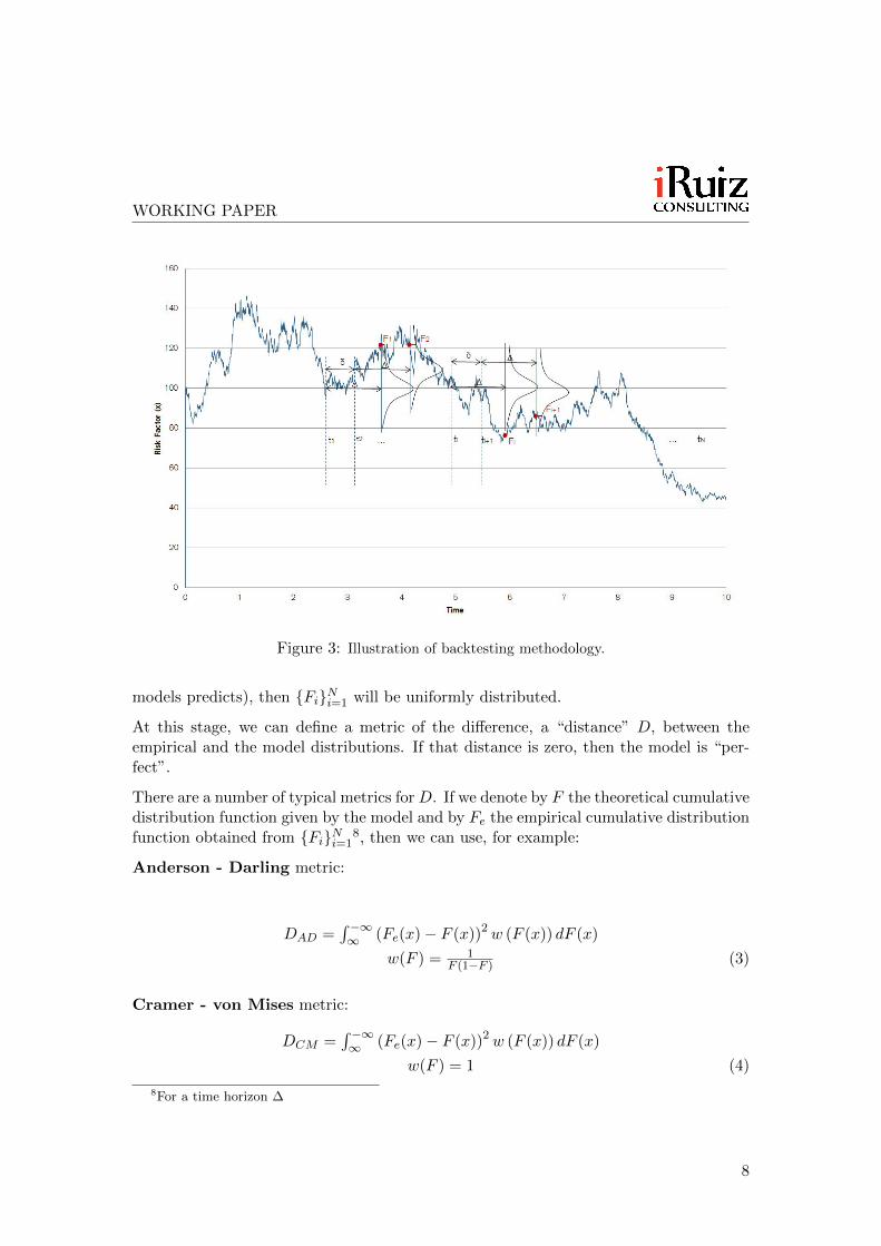
Backtesting an RFE means comparing the distribution of the risk factor given by themodel over time with the distribution actually seen in the market. In other words, wewant to check how the RFE measure and the observed “real” measure compare to eachother.

To do this6, we are going to consider the realized path (a time series) of the risk factorto be tested. That path is given by a collection of (typically daily) values xti . We willset a time point in that time series where the backtest starts (tstart), and a time pointwhere it ends (tend). The backtest time window is then T = tend − tstart. Then, if ∆ isthe time horizon over which we want to test our model (e.g. ∆ = 1 month), we proceedas follows (the reader can see in Figure 3 an illustration of this process):

1. The first time point of measurement is t1 = tstart. At that point, we calculate themodel risk factor distribution at a point t1 + ∆ subject to the realization of xt1 ;this can be done analytically if possible, or numerically otherwise. We then takethe realized value xt1+∆ of the time series at t1 + ∆ and observe where that valuefalls in the risk factor cumulative distribution calculated previously. This yields avalue F1

7.

2. We then move forward to t2 = t1 + δ. We calculate the risk factor distribution att2 + ∆ subject to realization of xt2 , and proceed as before: we observe where inthe model distribution function xt2+∆ falls and obtain F2 from it.

3. We repeat continuously the above until ti + ∆ reaches tend.

The outcome of this exercise is a collection {Fi}Ni=1 where N is the number of time stepstaken.

The key point in this methodology is the following: in the case of a “perfect” model (i.e.,if the empirical distribution from the time series is the same as the distribution that the

6Here the author follows Kenyon 2012 [4]7For the sake of clarity, the reader should note that Fi ∈ (0, 1) ∀i.

7

WORKING PAPER

Figure 3: Illustration of backtesting methodology.

models predicts), then {Fi}Ni=1 will be uniformly distributed.

At this stage, we can define a metric of the difference, a “distance” D, between theempirical and the model distributions. If that distance is zero, then the model is “per-fect”.

There are a number of typical metrics for D. If we denote by F the theoretical cumulativedistribution function given by the model and by Fe the empirical cumulative distributionfunction obtained from {Fi}Ni=1

8, then we can use, for example:

Anderson - Darling metric:

DAD =∫ −∞∞ (Fe(x)− F (x))2w (F (x)) dF (x)

w(F ) = 1F (1−F ) (3)

Cramer - von Mises metric:

DCM =∫ −∞∞ (Fe(x)− F (x))2w (F (x)) dF (x)

w(F ) = 1 (4)

8For a time horizon ∆

8

WORKING PAPER

Kolmogorov - Smirnov metric:

DKS = supx|Fe(x)− F (x)| (5)

Each metric will deliver a different measurement of D. Which of them is the mostappropriate depends on how the model being tested is actually used. This decision hassome degree of subjectivity by the researcher and practitioner9.

Having chosen a metric, we can compute now a value D̃ that measures how good themodel is.

The following questions arise now:

1. How large does D̃ need to be to indicate that a model is bad? Or, equivalently,how close to zero must it be to indicate that our model is good?

2. N is a finite number, so D̃ will never be exactly zero even if the model wereperfect10. How can we assess the validity of D̃?

In order to answer those two questions, we can proceed as follows. Let’s construct anartificial time series using the model being tested, and then apply our above procedureto it, yielding a value D11. The constructed time series will follow the model perfectly bydefinition, but D will not be exactly zero. This deviation will only be due to numerical“noise”. If we repeat this exercise a large number of times (M), we will obtain a collection{Dk}Mk=1, all of them compatible with a “perfect” model. That collection of D’s willfollow a certain probability distribution ψ(D) that we can approximate numericallyfrom {Dk}Mk=1 by making M sufficiently large.

Now, having obtained ψ(D), we can asses the validity of D̃: if D̃ falls in a range withhigh probability with respect to ψ(D), then the model is likely to be accurate, andvice-versa12.

The Three Bands

We are now in a position to extend the clear Basel framework established for marketrisk to the setting of counterparty risk. If we define Dy and Dr respectively as the

9For example, in risk management we are most interested in the quality of the models in the tails ofthe distribution, so we may want to use the Anderson - Darling metric. In capital calculations we areinterested in the whole of the distribution function, so we may want to use Cramer - von Mises. If we arehappy with small general deviations, but never large deviations, then we may want to use Kolmogorov- Smirnov.

10Zero is attained in the limit: limN→∞D = 0.11That artificial time series must have exactly the same time data as the empirical collection of values

xti .12Strictly speaking, what we can say is that if D̃ falls in a range with high probability in ψ(D), then

the model is compatible with a “perfect” models with high probability.

9

WORKING PAPER

95th and 99.99th percentiles of ψ(D), then we can define three bands for the modelperformance:

• Green band if D̃ ∈ [0, Dy)

• Yellow band if D̃ ∈ [Dy, Dr)

• Red band if D̃ ∈ [Dr,∞)

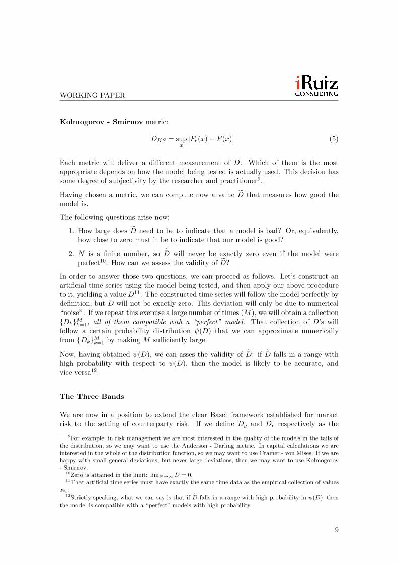
This is illustrated in Figure 4 for a simple Geometric Brownian Motion model. Withthis three-band approach, a financial institution can easily score a model and proceedas found appropriate.

Figure 4: Illustrative example of the distribution of D’s compatible with the model.

Examples

We now present a few examples where the mechanics of the methodology are illustrated.The Cramer - von Mises metric was used. Further examples can be found in the AppendixA.

Model with wrong skew

We want to see how the algorithm responds when the skew of the data and the modelare different. For this, the author generated an empirical time series with a GBM plus1-sided Poisson jump process that is taken as the empirical time series, and then it wastested against a simple GBM model with the same volatility as the time series13.

13The empirical time series had a volatility of 34%, a skew of -0.35 and an excess kurtosis of 0.54. TheGBM model had a volatility of 34%.

10

WORKING PAPER

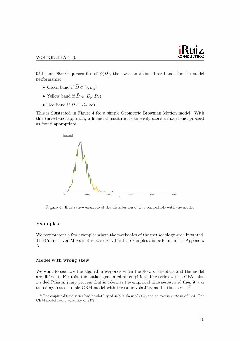
Figure 5 shows how the model responded14. In this specific example, the empirical timeseries has larger negative skew than the model. This is most visible in the UniformDistribution graphs (bottom panels).

Figure 5: Illustrative example of how the backtest algorithm behaves when the model skew isdifferent to the empirical skew.

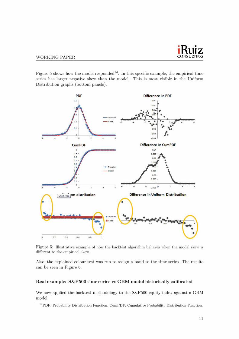
Also, the explained colour test was run to assign a band to the time series. The resultscan be seen in Figure 6.

Real example: S&P500 time series vs GBM model historically calibrated

We now applied the backtest methodology to the S&P500 equity index against a GBMmodel.

14PDF: Probability Distribution Function, CumPDF: Cumulative Probability Distribution Function.

11

WORKING PAPER

Figure 6: ψ(D) (blue) and D̃ (red dot) for a GBM-plus-jump time series tested against a GBMmodel with the same volatility as the time series.

Before proceeding with the results, an important remark needs to be made:

Model Calibration A counterparty risk RFE model is more than a set of stochasticequations. It actually consists of (i) a set stochastic equations (e.g. GBM diffusion plusPoisson jumps), (ii) a calibration methodology (e.g. 3-year historic volatility, impliedvolatility, etc) and (iii) a calibration frequency. The backtesting algorithm must considerall those inputs. For example, if the RFE is a GBM model which is calibrated quarterly,with a volatility equal to the annualized standard deviation of the daily log-returns forthe past 3 years, then the volatility of the GBM process must be recalibrated quarterlywhen we calculate D̃ and when we generate each of the M paths leading to ψ(D). It isvery important to use the same calibrating methodology and frequency in the backtestingexercise as we use in the live system.

This point was left out in the first explanation of the backtesting methodology for sim-plification of the explanation, but from now on, we will refer to the calibration periodas Tc (if historically calibrated), and to the calibrating frequency as δc.

Having said that, we are now going to apply the backtesting algorithm to the S&P500time series, using the daily time series from 2000 to 2011. The model we backtest is asimple GBM, with historical daily (δc = 1 day) calibration and volatility equal to theannualized standard deviation of log-returns for different calibrating windows Tc. Wewant to test how the model performs for time horizons ∆ of 10 days and one year, andfor calibrating windows Tc of three months and three years.

The following table summarizes the scores in terms of color bands:

12

WORKING PAPER

Tc = 3 months Tc = 3 years

∆ = 10 days GREEN YELLOW∆ = 1 year GREEN GREEN

Figure 7: Backtest measurements for S&P500 from 2000 to 2011.

When the model time horizon ∆ is short (10 days), a short calibration window (Tc =3 months) makes the model score a green, but when the calibrating window is long(Tc = 3 years), then the algorithm captures that there is a problem with the methodologyand the model scores a yellow15. However, when the model time horizon ∆ is long (1year), then the backtest indicates that either calibration window of 3 months or 3 yearsis good; both have a green score. This can be seen in Figure 7

Practical Considerations

Let’s discuss some important practical considerations.

On autocorrelation - the role of δ

If δ < ∆, there is autocorrelation in the collection {Fi} by construction. However,that autocorrelation also exists in the construction of ψ(D). Hence the methodologyneutralizes this effect “automatically”. As such, as long as the values of T , ∆, and δare the same in the calculations of D̃ and of ψ(D), we do not need to do any further

15The problem is that 3-year historical volatility is not a good predictor of short-term future volatility.

13

WORKING PAPER

adjustments to compensate for the induced autocorrelation. This autocorrelation effectis discussed in more detail in Appendix B.

Maximum utilisation of available information - the role of ∆ and T

In practice, one of the big problems of counterparty risk backtesting is that historicaldata tends to be scarce: T is usually not long enough relative to the time horizon ∆ inwhich the model needs to be tested. As a result, there may be too few independent pointsin our test. For example, if we have a backtesting window T of 10 years and we want tomeasure a model’s performance with a ∆ of 2 years, we only have 5 independent points16.So, the statistical relevance of the backtest can be quite limited by construction.

This is intrinsic to CCR backtesting and, in the author’s opinion, there is no way toget away from it. However, this limitation is again captured in this methodology, as thewidth of the ψ(D) “automatically” expands as T/∆ decreases. This is because, when wecalculate ψ(D) in a set up where T/∆ is small, the algorithm will provide a wide range ofD’s compatible with the model, as the independent information is relatively scarce. Forthis reason this methodology seems to be optimal as it “automatically” makes most ofthe available information, however abundant or scarce it may be. This effect is discussedin more detailed in Appendix C.

What parameters to use

The proposed methodology has the following inputs:

• On the model side, we typically have a set of stochastic differential equations forthe RFE, a calibration methodology, and a calibration frequency.

• On the backtesting side, we have a time window T , a time horizon ∆, and a stepsize δ.

Given a model to be tested, how do we choose T , ∆ and δ?

T is firstly driven by the availability of good quality data. Once this is provided, itshould be large enough so we can have some statistical relevance in the algorithm, butnot too large so that the search for a good model becomes mission impossible17. Thereis no set rule to define what is too much or too little; in practice, this can only be leftto the experience and market knowledge of the researcher18.

16Assuming no auto-dependency in the data.17If there is sufficiently large amount of data, most models, if not all, will fail the backtest. See

Appendix D for more details.18In reality, the practitioner should not worry to much about this at first, as the constrain here tends

to be lack of available good data, and so this problem is not even seen in most cases.

14

WORKING PAPER

∆ will be determined from the typical tenor of the trades in the portfolio under testing,subject to availability of data. It should cover a range of values up to the typical maturityof the portfolio being tested - no need to test a ∆ beyond 5 years, for example, if mostof the portfolio affected by the RFE matures in 5 years. In this case the author wouldsuggest ∆ of one day, one week, twp weeks, one month, three months, six months, oneyear, two years, three years and five years, with special attention to those ∆ where therisk of the portfolio tends to peak.

Regarding δ, the author recognises that it is not clear him what is ideal, but someanecdotal evidence19 suggests that there is no reason to make the value of δ smallerthan ∆, hence making the algorithm slower, unless T/∆ is small and non-integer.

Further details on this subject can be found in the Appendix D.

Multiple-∆ scores V. Single-∆ score

In order to assess the validity of a model for CCR, we should test it not only for anumber of representative time horizons ∆, as just explained, but also for a number ofrepresentative risk factors (e.g., several FX rates for an FX model). As a result we caneasily end up with up to a few hundred colour scores.

We could have the temptation of building a final aggregated score based on those manysub-scores, but in the author’s opinion and experience this will be difficult to managein practice as the granularity of the analysis can get lost. In reality, he has found mostpractical to build a coloured table with the most representative scores, not more thanone hundred, find patterns in it (e.g., most emerging market currencies fail for ∆ greaterthan 2 year) and modify the model as needed until most scores are green and/or we canexplain and manage those yellow and red scores. More details can be found in AppendixE.

Numerical approximations

The calculation of D will be done numerically using a number of approximations. Thiswill introduce some noise in these calculations. However, the same noise will be in-troduced in the calculation of ψ(D) and, hence, this noise is, also, “automatically”considered in the assessment of D̃.

Asset Class Agnostic

This methodology can be applied to any asset class: interest rates, foreign exchange,equities, commodities, credit, etc. There are no limitations in this respect.

19See Appendix D.

15

WORKING PAPER

Backtest of dependency structures

The methodology can be applied to individual risk factors or to sets of risk factors inparallel by extending the methodology to many-dimensions. In that case, the procedurewill also test the dependency structure of the model against the “real” one existing inthe data. This is discussed in more detail in the Appedix F.

Testing the whole probability distribution

Often, risk management uses a given percentile in the distribution function to measurecounterparty risk (e.g., 95% PFE20). For this reason, sometimes risk models are testedby counting the number of exceptions outside of a given percentile envelopes. However,that methodology is sub-optimal for regulatory capital models where the key measureof risk is the EPE21. This is because EPE is an average measure and, as such, to checkits validity we need to test the quality of the whole distribution functions of exposures,not only exceptions above or below a given percentile. In fact, the framework explainedin this paper can easily be adapted to test specific parts of the probability distributionby changing the weight function w(F ).

Structural changes in the market

The explained methodology provides a score for a model during a time period T , butif that period contains a structural change in the market (e.g., 2008), it provides noinformation what-so-ever as to how the model reacted to capture those changes. A wayto do this is buy performing a “rolling window” test. In this test, we can do the testwith a relatively small window Trw that we then roll over the period T . If we definea parameter Z as D̃ over a critical Dc, where Dc can be the D value that marks thefrontier between the green and yellow bands, then we can have a time series Zt overthe testing window T from where we can easily assess the model performance duringstructural changes in the markets: when Zt < 1 the model is good, but when Zt > 1 themodel is having problems22.

Further details can be found in the Appendix G.

Historic V. implied model calibrations

Risk models tend to be calibrated historically, but pricing models (e.g., CVA) tend tohave market-implied calibrations. The proposed backtesting methodology is agnostic tothe type of calibration in the model. The only thing that the researcher must bear in

20Potential Future Exposure.21The same could be applied to CVA if it was to be backtested.22If wanted, the same study can be done with Dc being the frontier between the yellow and red bands.

16

WORKING PAPER

mind is that the same calibration methodology must be applied to compute both D̃ andψ(D). In the case of market-implied calibration, this will require a joint model for theRFE and the calibration variables.

Conclusions

The author has proposed a backtesting framework for Counterparty Credit Risk modelsthat provides a set of green/yellow/red scores to a model, resembling the widely used ap-proach in the market risk area. On this way, a model receives a colour score for each timehorizon ∆ and relevant risk factor that enables proper good model management.

There are a number of important factors to consider. First, a “distance metric” Dbetween the empirical and the model distribution functions needs to be chosen. Then, atime window T needs to be picked; in most cases, this time window will be determinedby the availability of data. The time horizons ∆ need to be chosen by considering thematurities of the portfolio being tested. Also the most significant risk factors for theportfolio need to be considered. Finally, δ should arguably be chosen equal to ∆, exceptwhen T/∆ is small and non-integer.

We have seen how this methodology maximizes the utilization of available informationand it can be applied to any asset-class and calibrating methodology.

The author has successfully implemented this methodology in tier-one banking environ-ments.

Acknowledgements

The author would like to thank Ahmed Aichi, Piero Del Boca, Chris Kenyon and ChrisMorris for interesting comments and remarks to this piece of work.

Appendix

A Examples

Model with wrong volatility

We want to gain some understanding as to how the algorithm performs when the em-pirical data has a different volatility to that assumed by the model. In order to achievethis, we simulate a time series using a GBM process and treat it as the empirical data;

17

WORKING PAPER

on this way, the inputs to the algorithm is well known and the output can be understoodin detail.

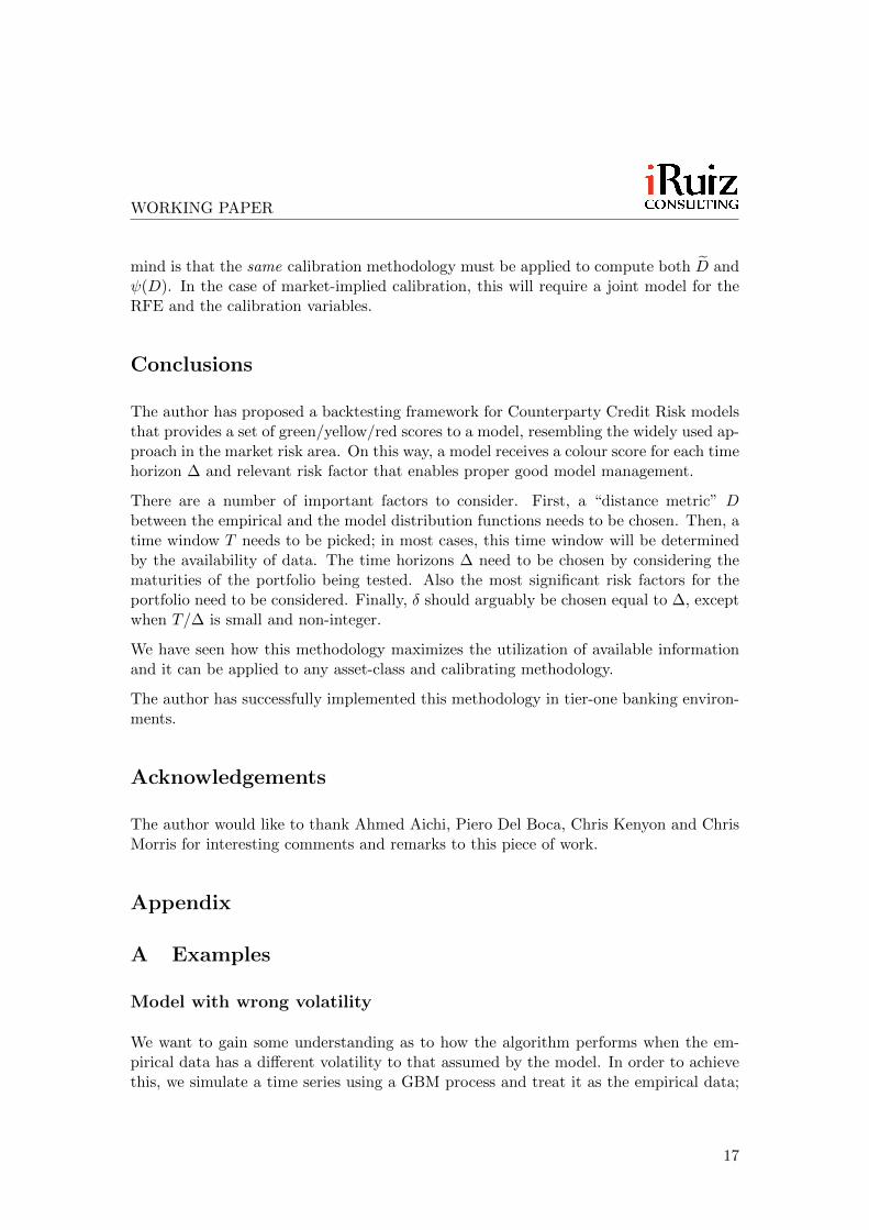
Figure 8 shows the output of the backtest algorithm when the empirical volatility islower than the model volatility. In those graphs, the data obtained from the model hasbeen fitted to a standard normal distribution function, and the empirical data has alsobeen normalized using the same normalization factors as for the model. As a result,the graphs illustrate the difference between the empirical and the model distributionfunctions. If the model were to fit the empirical data “perfectly”, then both graphs(blue and red) should lie on top of each other.

Figure 8: Illustrative example of how the backtest algorithm behaves when the model volatilityis higher than the empirical volatility.

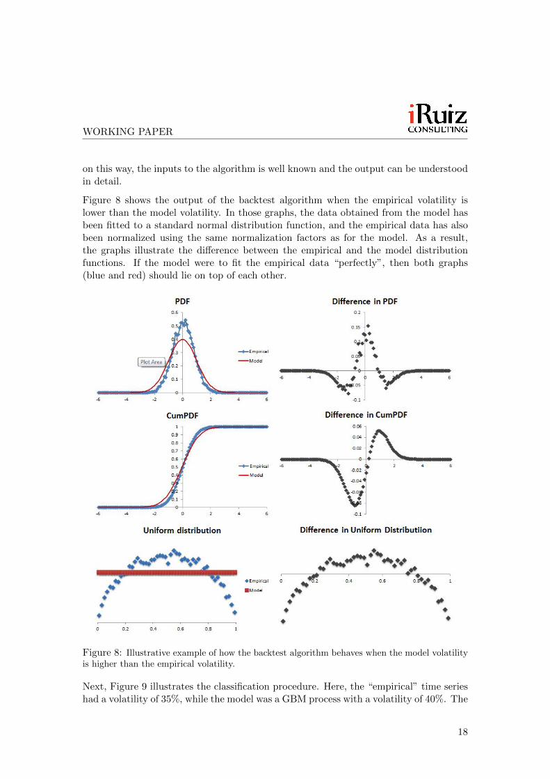
Next, Figure 9 illustrates the classification procedure. Here, the “empirical” time serieshad a volatility of 35%, while the model was a GBM process with a volatility of 40%. The

18

WORKING PAPER

backtest procedure yielded D̃ = 0.003, while the red band for this backtesting exercisestarts at 0.0018; hence, the algorithm classifies this model into the red band for the timeseries, indicating that it is inaccurate.

Figure 9: ψ(D) (blue) and D̃ (red dot) for a GBM-driven time series tested against a GBMmodel with a higher volatility.

Model with wrong kurtosis

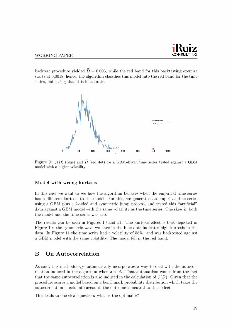
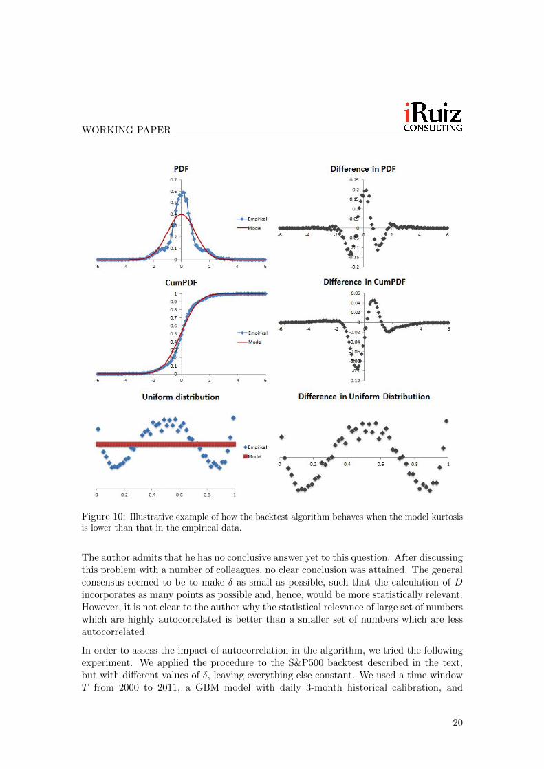
In this case we want to see how the algorithm behaves when the empirical time serieshas a different kurtosis to the model. For this, we generated an empirical time seriesusing a GBM plus a 2-sided and symmetric jump process, and tested this “artificial”data against a GBM model with the same volatility as the time series. The skew in boththe model and the time series was zero.

The results can be seen in Figures 10 and 11. The kurtosis effect is best depicted inFigure 10: the symmetric wave we have in the blue dots indicates high kurtosis in thedata. In Figure 11 the time series had a volatility of 58%. and was backtested againsta GBM model with the same volatility. The model fell in the red band.

B On Autocorrelation

As said, this methodology automatically incorporates a way to deal with the autocor-relation induced in the algorithm when δ < ∆. That automatism comes from the factthat the same autocorrelation is also induced in the calculation of ψ(D). Given that theprocedure scores a model based on a benchmark probability distribution which takes theautocorrelation effects into account, the outcome is neutral to that effect.

This leads to one clear question: what is the optimal δ?

19

WORKING PAPER

Figure 10: Illustrative example of how the backtest algorithm behaves when the model kurtosisis lower than that in the empirical data.

The author admits that he has no conclusive answer yet to this question. After discussingthis problem with a number of colleagues, no clear conclusion was attained. The generalconsensus seemed to be to make δ as small as possible, such that the calculation of Dincorporates as many points as possible and, hence, would be more statistically relevant.However, it is not clear to the author why the statistical relevance of large set of numberswhich are highly autocorrelated is better than a smaller set of numbers which are lessautocorrelated.

In order to assess the impact of autocorrelation in the algorithm, we tried the followingexperiment. We applied the procedure to the S&P500 backtest described in the text,but with different values of δ, leaving everything else constant. We used a time windowT from 2000 to 2011, a GBM model with daily 3-month historical calibration, and

20

WORKING PAPER

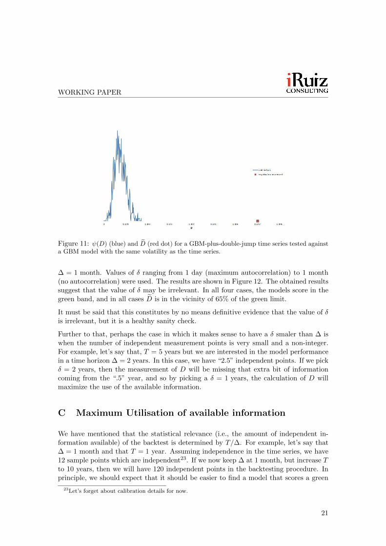
Figure 11: ψ(D) (blue) and D̃ (red dot) for a GBM-plus-double-jump time series tested againsta GBM model with the same volatility as the time series.

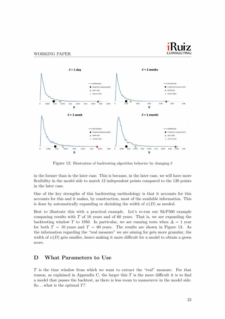
∆ = 1 month. Values of δ ranging from 1 day (maximum autocorrelation) to 1 month(no autocorrelation) were used. The results are shown in Figure 12. The obtained resultssuggest that the value of δ may be irrelevant. In all four cases, the models score in thegreen band, and in all cases D̃ is in the vicinity of 65% of the green limit.

It must be said that this constitutes by no means definitive evidence that the value of δis irrelevant, but it is a healthy sanity check.

Further to that, perhaps the case in which it makes sense to have a δ smaler than ∆ iswhen the number of independent measurement points is very small and a non-integer.For example, let’s say that, T = 5 years but we are interested in the model performancein a time horizon ∆ = 2 years. In this case, we have “2.5” independent points. If we pickδ = 2 years, then the measurement of D will be missing that extra bit of informationcoming from the “.5” year, and so by picking a δ = 1 years, the calculation of D willmaximize the use of the available information.

C Maximum Utilisation of available information

We have mentioned that the statistical relevance (i.e., the amount of independent in-formation available) of the backtest is determined by T/∆. For example, let’s say that∆ = 1 month and that T = 1 year. Assuming independence in the time series, we have12 sample points which are independent23. If we now keep ∆ at 1 month, but increase Tto 10 years, then we will have 120 independent points in the backtesting procedure. Inprinciple, we should expect that it should be easier to find a model that scores a green

23Let’s forget about calibration details for now.

21

WORKING PAPER

Figure 12: Illustration of backtesting algorithm behavior by changing δ

in the former than in the later case. This is because, in the later case, we will have moreflexibility in the model side to match 12 independent points compared to the 120 pointsin the later case.

One of the key strengths of this backtesting methodology is that it accounts for thisaccounts for this and it makes, by construction, most of the available information. Thisis done by automatically expanding or shrinking the width of ψ(D) as needed.

Best to illustrate this with a practical example. Let’s re-run our S&P500 examplecomparing results with T of 10 years and of 60 years. That is, we are expanding thebacktesting window T to 1950. In particular, we are running tests when ∆ = 1 yearfor both T = 10 years and T = 60 years. The results are shown in Figure 13. Asthe information regarding the “real measure” we are aiming for gets more granular, thewidth of ψ(D) gets smaller, hence making it more difficult for a model to obtain a greenscore.

D What Parameters to Use

T is the time window from which we want to extract the “real” measure. For thatreason, as explained in Appendix C, the larger this T is the more difficult it is to finda model that passes the backtest, as there is less room to manoeuvre in the model side.So. . . what is the optimal T?

22

WORKING PAPER

Figure 13: Backtest measurements for S&P500 from 2000 to 2011 (top) and from 1950 to 2011(bottom).

First of all, a practical constraint in this regard is the availability of good quality data;often, data does not date as far back as we would like it to, and when it does, it oftenlacks quality. If that problem is solved, on the one hand, T should be long enough(relative to ∆) so that the backtest algorithm has statistical relevance. On the otherhand, large values of T will make the task of building a model difficult to a degree thatcould be impractical.

In the author’s view, unfortunately there is no set rule for the optimal T . In practice,the researcher and practitioner will have to balance out all these constrains to come upwith a view on the optimal T .

∆ represents the time horizon in which we want to test the model. In this case, there isa clear optimal value for the maximum ∆. It will be determined by the maturity of theportfolios affected by the RFE under testing. For example, if we want to test a foreignexchange model for a portfolio with most of the trades maturing in less than 3 years,then it is not necessary to test the RFE beyond 3 years. This can cause some practical

23

WORKING PAPER

problems, as there are some asset classes where the typical length of a portfolio can bemuch larger than the available data; e.g., inflation, where trade tenors tend to be ataround 25 years and can even go up to 50 years. In such cases, it is impossible to do agood backtest and all we can can do is to test the model for shorter time horizons andmake sure that the long-term RFE behavior is reasonable. Given a maximum ∆, weshould test our model in a representative range of values from one day to that maximum∆.

δ represents the granularity in the backtesting calculation. As discussed in Appendix B,it is not clear to the author whether a small δ is better “per se”. If T is sufficiently large toguarantee statistical relevance with independence between time points in the time series,then the author suggests to use the smallest δ which guarantees independence. If there isno autocorrelation in the time series, this means that δ = ∆; otherwise, δ = ∆+τ , whereτ is the minimum time needed for the autocorrelation effects to disappear. However, asexplained in Appendix B, the case in which the algorithm will benefit from a smaller δis when T/∆ is small and non-integer.

E Multiple-∆ scores V. single-∆ score

A practical consequence of the mutiple ∆’s that we need to use in the test is that amodel will not have one score, but a collection of them, one per ∆. Typically, we wouldhave between 5 to 10 ∆’s.

Further to that, in reality we should have a number of those collections, as an RFEshould be tested against several relevant risk factors. For example, an FX RFE willtypically need to be tested against all major currencies (USD, GBP, EUR, CHF, JPY)and against all other currencies significantly relevant to the financial institution. Ingeneral, we may have ten to thirty risk factors to test.

As a result, we will end up with between 50 and 30 scores for the model. How could beproceed to make these measurements useful?

We could define an overall score, using some formula that agregate all those scores intoa single one. However, in the author’s view and experience, this will have quite a limiteduse, as the granular information provided by the analysis will be too hidden. In his view,the best way to proceed is as follows:

1. Produce one single sheet with a table showing, with colours, scores for all ∆’s andrisk factors. Ideally, we do not want more than 100 scores. In this table, we willhave some green, some yellow and some red boxes. This gives a very good eye-ballsnap shot of the model performance. We are aiming at lots of green, some yellowand perhaps, a few red boxes.

2. Find patterns in the yellow and red boxes. For example, “red scores tend to happenin emerging market currencies for ∆ greater than 2 years”.

24

WORKING PAPER

3. Based on those patterns, try to modify the model so that those yellow and redboxes tend towards the green.

4. Proceed in a loop in the previous steps until we have mostly green boxes.

5. Finally, find the reason behind the remaining non-green scores, if they exist; e.g.,poor quality data, a currency linked to a government default, etc. Then estimatethe impact of those exceptional cases in your portfolio and assess the need of aspecial process for those cases in the organisation.

In the author’s experience, this is the optimal way to develop an RFE model thatbacktests well.

F Backtest of Dependency Structures

Let’s say that we have a model for a curve consisting of a number of tenor points, whichhave a certain dependency structure (e.g., a yield curve). We have historical time seriesfor each of those points. Testing the RFE of each point in the curve, in isolation tothe rest, will provide no information what-so-ever as to the quality of the model withregards to the dependency structure between those points.

In this paper we have seen how to apply the explained procedure in the context of onerisk factor. However, this methodology can be extended to a multi-dimensional case inwhich the dependency between risk factors is also tested. This can be done by expandingthe calculation of D to multi-dimensions. The color scheme can be applied in exactlythe same way as in the one-dimensional case. This way, the backtest can include, forexample, the validity check for a copula structure.

For example, we can expand the Anderson - Darling metric to two dimensions as fol-lows:

D′AD =∫ −∞∞

∫ −∞∞ (Fe(x, y)− F (x, y))2w (F (x, y)) dF (x, y), w(F ) = 1

F (1−F )

In practice, this calculation can become quite convoluted, so it must be made with a lotof care. The author suggests that models be first tested in one dimension. Then, multi-dimensional tests can be implemented. This way, should the final joint-RFE test be non-satisfactory, potential problems can be better isolated, identified and managed.

G Structural Changes in the Market

The markets undergo periods of stress from time to time. The most recent one startedin the credit asset class in 2007. These phenomena occurs for a number of reasons whichtend to gravitate around wrong economic fundamentals, markets drying out, importantimbalances in the size and/or price of markets, human ”manias”, etc. Interestingly, after

25

WORKING PAPER

these events occur, it is “easy” to make sense of them, but very few people are able toforesee them. In some cases, it is impossible by definition24.

Stochastic models cannot capture these events, they are not build for that. But weideally want models which react quickly to changing market conditions and which arevalid for a wide range of market environments25. Because of that, assessing the qualityof an EPE model requires also assessing how the model behaves under structural changesin the markets.

The proposed backtesting methodology can help in that respect by implementing arolling window test, in which T is kept constant and is rolled over time.

For example, let’s say we have a credit model which we are testing in the 2000 to2012 window and that receives a green score. What that means is that the explainedmethodology provides a green score to the overall performance of the model in the periodT , but it gives no indication as to how the model performed during the 2007-09 crisis.In order to assess this, we can

1. Implement a window T of 2 years starting in 2000 and roll it forward up to 2010,obtaining a rolling D̃t.

2. In each of those rolling tests, record the critical value Dcg,t that sets the frontier

between the green and the yellow band, and Dcr,t that sets the frontier between the

yellow and the rend band.

3. Finally, divide each D̃t by each Dc to obtain a time series of rolling scores, thatwe are going to call Z-scores: Zg,t and Zr,t.

If Zg,t < 1, the model is in the green band, but when it goes over that value, the modelgoes into the yellow or red band. A parallel analysis can be done with Zr,t. On thisway, by plotting each time series Zt, the researcher can assess the quality of the modelresponse to changing market conditions and, when the quality decreases, have an ideaof how bad the problem is.

In fact, the author has seen precisely this kind of behaviour in the backtesting workhe has done for one of his clients. There, a model was backtested for the 2001 to 2011period. Overall, the model scored a green. A rolling window test, with T = 2 years and∆ = 1 month, showed how the model started in the green band, went to the yellow/redbands when the backtesting period overlapped with the peak of the credit crunch, andthen went back to green when the (historical) calibration window overlapped sufficientlywith the credit crunch. This test showed that the model was not good at coping withstructural changes in the market (as expected as it was historically calibrated) but it

24These are the now called Black Swan events[5].25We can certainly build a model which gives a certain probability to certain stress events in the

future. However all we will achieve with this is that some scenarios in our Monte Carlo simulation willfollow those stress events, but the impact in the “average” scenario will be limited in general. For thisreason, risk management uses Potential Future Exposure or Expected Shortfall risk measures to monitorthe so-called tail risk.

26

WORKING PAPER

was good both for quiet and stress regimes once the calibration accounted for it. As aresult, the institution implemented a special stress process to cover the risk of suddenchanges in the market but it was shown that there was not need for a different modelfor stressed market conditions.

References

[1] Supervisory framework for the use of “backtesting” in conjunction with the internal mod-els approach to market risk captial requirements, tech. rep., Basel Committee of BankingSupervision, 1996.

[2] Sound practices for backtesting counterparty credit risk models, tech. rep., Basel Committeeof Banking Supervision, 2010.

[3] E. Canabarro, Counterparty Credit Risk, Risk Books, first ed., 2009.

[4] C. Kenyon, Model risk in risk factor evolution, in Measuring and Controlling Model Risk,London, 2011.

[5] N. N. Taleb, The Back Swah: the Impact of the Highly Improbable, Penguin Books, first ed.,2008.

27