Backpropagation Network Structure
36
November 26, 2013 Computer Vision Lecture 15: Object Recognition III 1 Backpropagation Network Structure Perceptrons (and many other classifiers) can only linearly separate the input space. Backpropagation networks (BPNs) do not have this limitation and can in principle find any statistical relationship between training inputs and desired outputs. The training procedure is computationally complex. BPNs are multi-layered networks. It has been shown that three layers of neurons are sufficient to compute any function that could be useful for, for example, a
-
Upload
germane-blevins -
Category
Documents
-
view
44 -
download
0
description
Backpropagation Network Structure. Perceptrons (and many other classifiers) can only linearly separate the input space. Backpropagation networks (BPNs) do not have this limitation and can in principle find any statistical relationship between training inputs and desired outputs. - PowerPoint PPT Presentation
Transcript of Backpropagation Network Structure
November 26, 2013 Computer Vision Lecture 15: Object Recognition III
1
Backpropagation Network StructurePerceptrons (and many other classifiers) can only linearly separate the input space.
Backpropagation networks (BPNs) do not have this limitation and can in principle find any statistical relationship between training inputs and desired outputs.
The training procedure is computationally complex.
BPNs are multi-layered networks. It has been shown that three layers of neurons are sufficient to compute any function that could be useful for, for example, a computer vision application.
November 26, 2013 Computer Vision Lecture 15: Object Recognition III
2
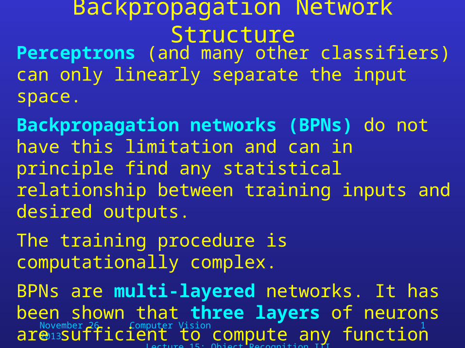
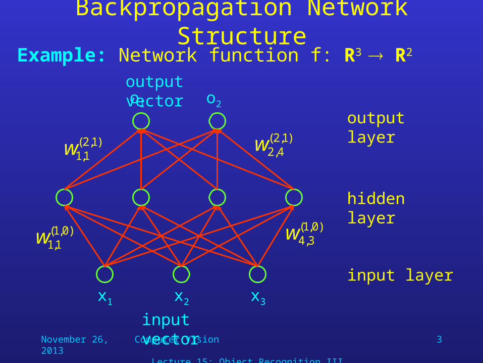
Backpropagation Network StructureMost backpropagation networks use the following three layers:
• Input layer: Only stores the input and sends it to the hidden layer; does not perform computation.
• Hidden layer: (i.e., not visible from input or output side) receives data from input layer, performs computation, and sends results to output layer.
• Output layer: Receives data from hidden layer, performs computation, and its results form the network’s output.
November 26, 2013 Computer Vision Lecture 15: Object Recognition III
3
Backpropagation Network StructureExample: Network function f: R3 R2
output layer
hidden layer
input layer
input vector
output vector
x1 x2
o2o1
x3
)1,2(1,1w
)1,2(4,2w
)0,1(1,1w
)0,1(3,4w
November 26, 2013 Computer Vision Lecture 15: Object Recognition III
4
The Backpropagation Algorithm
Idea behind backpropagation learning:
Neurons compute a continuous, differentiable function function between their input and output.
We define an error of the network output as a function of all the network’s weights.
Then find those weights for which the error is minimal.
With a differentiable error function, we can use the gradient descent technique to find the absolute minimum of the error function.
November 26, 2013 Computer Vision Lecture 15: Object Recognition III
5
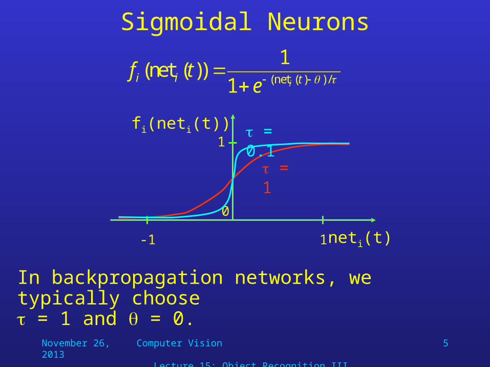
Sigmoidal Neurons
In backpropagation networks, we typically choose = 1 and = 0.
1
0
1
fi(neti(t))
neti(t)-1
= 1
= 0.1
/))(net(1
1))(net(
tii ietf
November 26, 2013 Computer Vision Lecture 15: Object Recognition III
6
Sigmoidal Neurons
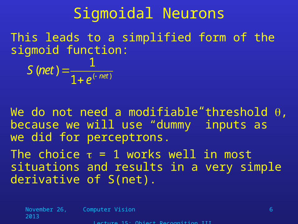
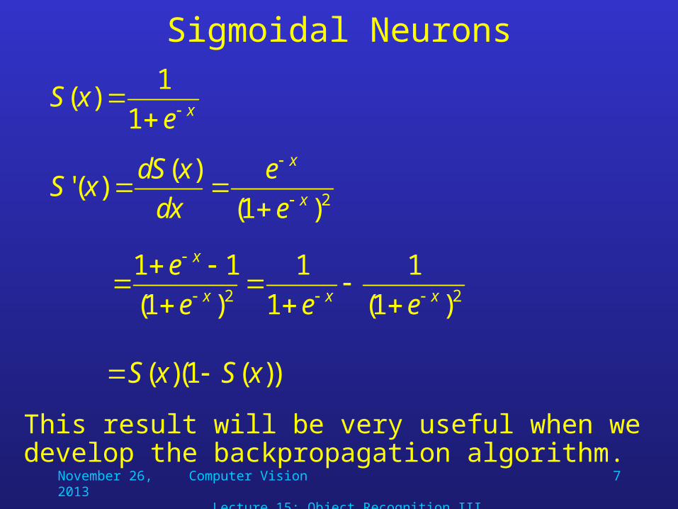
This leads to a simplified form of the sigmoid function:
We do not need a modifiable threshold , because we will use “dummy” inputs as we did for perceptrons.
The choice = 1 works well in most situations and results in a very simple derivative of S(net).
)(1
1)(
netenetS
November 26, 2013 Computer Vision Lecture 15: Object Recognition III
7
Sigmoidal Neurons
This result will be very useful when we develop the backpropagation algorithm.
xexS
1
1)(
2)1(
)()('
x
x
e
e
dx
xdSxS
22 )1(
1
1
1
)1(
11xxx
x
eee
e
))(1)(( xSxS

November 26, 2013 Computer Vision Lecture 15: Object Recognition III
8
Gradient DescentGradient descent is a very common technique to find the absolute minimum of a function.
It is especially useful for high-dimensional functions.
We will use it to iteratively minimizes the network’s (or neuron’s) error by finding the gradient of the error surface in weight-space and adjusting the weights in the opposite direction.
November 26, 2013 Computer Vision Lecture 15: Object Recognition III
9
Gradient Descent
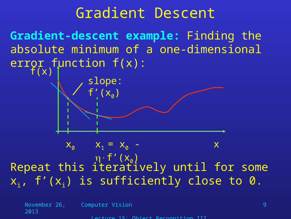
Gradient-descent example: Finding the absolute minimum of a one-dimensional error function f(x):
f(x)
xx0
slope: f’(x0)
x1 = x0 - f’(x0)
Repeat this iteratively until for some xi, f’(xi) is sufficiently close to 0.
November 26, 2013 Computer Vision Lecture 15: Object Recognition III
10
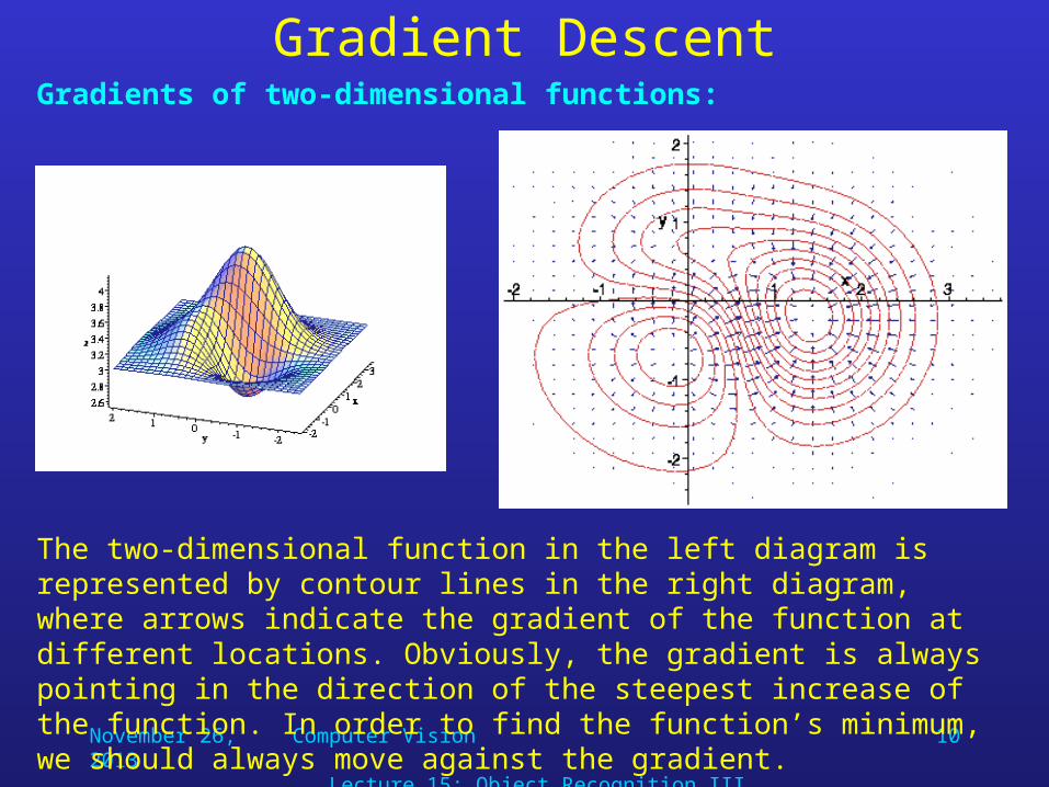
Gradient DescentGradients of two-dimensional functions:
The two-dimensional function in the left diagram is represented by contour lines in the right diagram, where arrows indicate the gradient of the function at different locations. Obviously, the gradient is always pointing in the direction of the steepest increase of the function. In order to find the function’s minimum, we should always move against the gradient.
November 26, 2013 Computer Vision Lecture 15: Object Recognition III
11
Backpropagation Learning
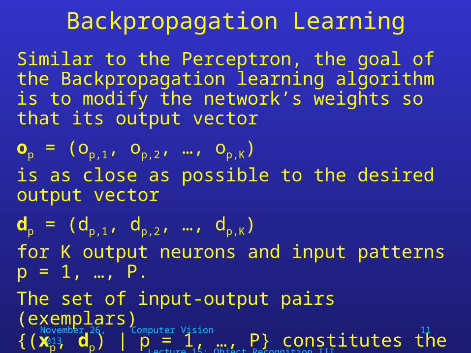
Similar to the Perceptron, the goal of the Backpropagation learning algorithm is to modify the network’s weights so that its output vector
op = (op,1, op,2, …, op,K)
is as close as possible to the desired output vector
dp = (dp,1, dp,2, …, dp,K)
for K output neurons and input patterns p = 1, …, P.
The set of input-output pairs (exemplars) {(xp, dp) | p = 1, …, P} constitutes the training set.
November 26, 2013 Computer Vision Lecture 15: Object Recognition III
12
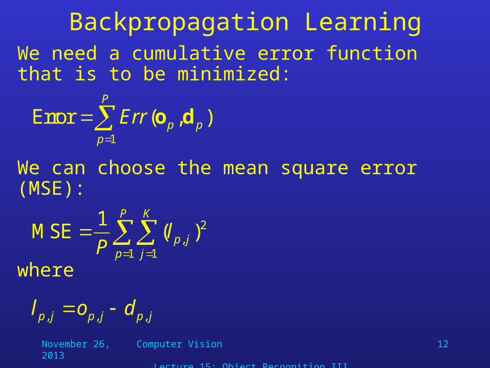
Backpropagation LearningWe need a cumulative error function that is to be minimized:
P
pppErr
1
),(Error do
We can choose the mean square error (MSE):
P
p
K
jjplP 1 1
2, )(
1MSE
where
jpjpjp dol ,,,
November 26, 2013 Computer Vision Lecture 15: Object Recognition III
13
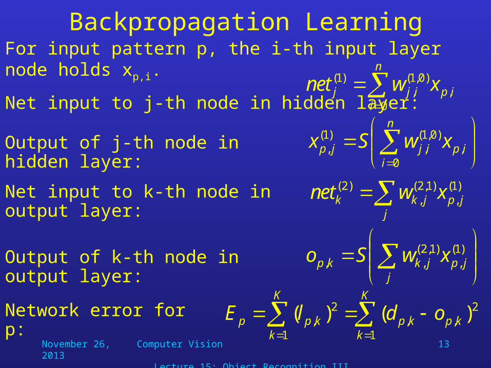
Backpropagation LearningFor input pattern p, the i-th input layer node holds xp,i.
Net input to j-th node in hidden layer:
n
iipijj xwnet
0,
)0,1(,
)1(
K
kkpkp
K
kkpp odlE
1
2,,
1
2, )()(Network error for p:
jjpjkkp xwSo )1(
,)1,2(
,,Output of k-th node in output layer:
j
jpjkk xwnet )1(,
)1,2(,
)2(Net input to k-th node in output layer:
n
iipijjp xwSx
0,
)0,1(,
)1(,Output of j-th node in hidden layer:
November 26, 2013 Computer Vision Lecture 15: Object Recognition III
14
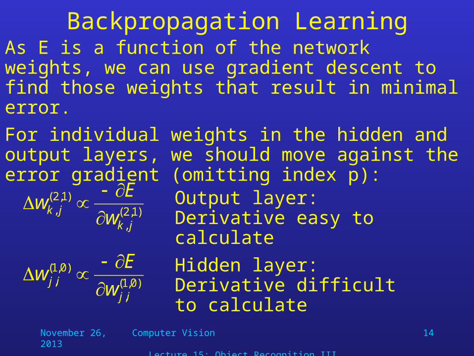
Backpropagation LearningAs E is a function of the network weights, we can use gradient descent to find those weights that result in minimal error.
For individual weights in the hidden and output layers, we should move against the error gradient (omitting index p):
)1,2(,
)1,2(,
jkjk w
Ew
)0,1(,
)0,1(,
ijij w
Ew
Output layer: Derivative easy to calculate
Hidden layer: Derivative difficult to calculate
November 26, 2013 Computer Vision Lecture 15: Object Recognition III
15
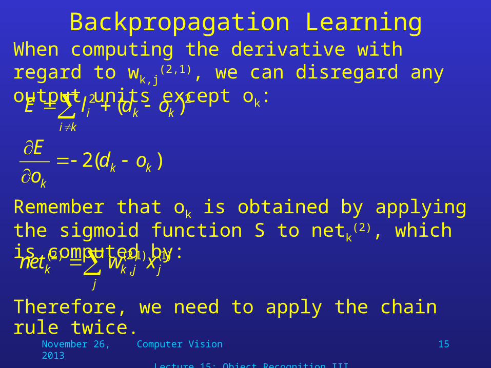
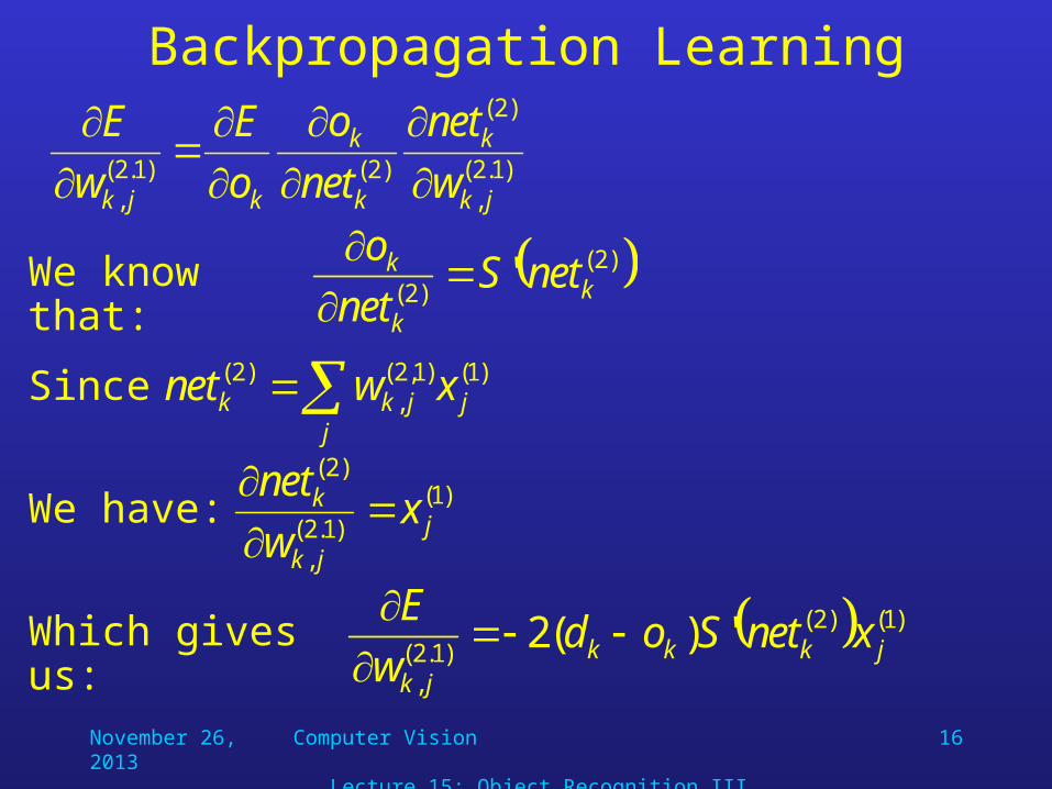
Backpropagation LearningWhen computing the derivative with regard to wk,j
(2,1), we can disregard any output units except ok:
ki
kki odlE 22 )(
)(2 kkk
odo
E
Remember that ok is obtained by applying the sigmoid function S to netk
(2), which is computed by:
j
jjkk xwnet )1()1,2(,
)2(
Therefore, we need to apply the chain rule twice.
November 26, 2013 Computer Vision Lecture 15: Object Recognition III
16
Backpropagation Learning
)1.2(,
)2(
)2()1.2(, jk
k
k
k
kjk w
net
net
o
o
E
w
E
Since j
jjkk xwnet )1()1,2(,
)2(
)1()1.2(
,
)2(
jjk
k xw
net
We have:
We know that: )2()2(
' kk
k netSnet
o
Which gives us: )1()2()1.2(
,
')(2 jkkkjk
xnetSodw
E
November 26, 2013 Computer Vision Lecture 15: Object Recognition III
17
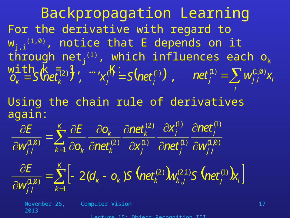
Backpropagation LearningFor the derivative with regard to wj,i
(1,0), notice that E depends on it through netj
(1), which influences each ok with k = 1, …, K:
Using the chain rule of derivatives again:
, )2(kk netSo
iiijj xwnet )0,1(
,)1( , )1()1(
jj netSx
)0,1(,
)1(
)1(
)1(
1)1(
)2(
)2()0,1(, ij
j
j
jK
k j
k
k
k
kij w
net
net
x
x
net
net
o
o
E
w
E
K
kijjkkkk
ij
xnetSwnetSodw
E
1
)1()1,2(,
)2()0,1(
,
'')(2
November 26, 2013 Computer Vision Lecture 15: Object Recognition III
18
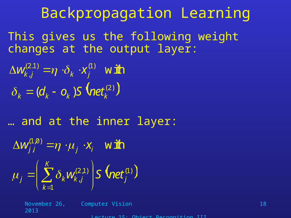
Backpropagation Learning
This gives us the following weight changes at the output layer:
… and at the inner layer:
with)1()1.2(, jkjk xw
)2(')( kkkk netSod
with)0,1(, ijij xw
)1(
1
)1,2(, ' j
K
kjkkj netSw
November 26, 2013 Computer Vision Lecture 15: Object Recognition III
19
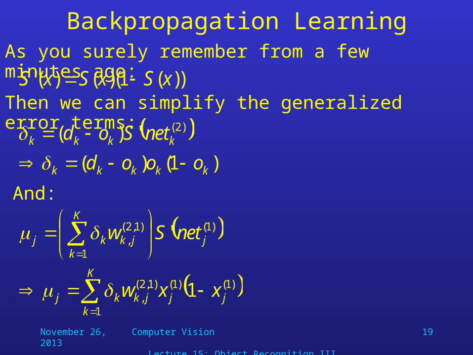
Backpropagation LearningAs you surely remember from a few minutes ago:
Then we can simplify the generalized error terms:))(1)(()(' xSxSxS
)2(')( kkkk netSod )1()( kkkkk oood
And:
)1(
1
)1,2(, ' j
K
kjkkj netSw
)1()1(
1
)1,2(, 1 jj
K
kjkkj xxw
November 26, 2013 Computer Vision Lecture 15: Object Recognition III
20
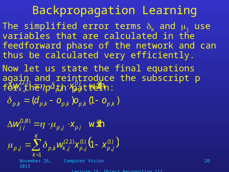
Backpropagation LearningThe simplified error terms k and j use variables that are calculated in the feedforward phase of the network and can thus be calculated very efficiently.
Now let us state the final equations again and reintroduce the subscript p for the p-th pattern:
with)1(,,
)1.2(, jpkpjk xw
)1()( ,,,,, kpkpkpkpkp oood
with,,)0,1(
, ipjpij xw
)1(,
)1(,
1
)1,2(,,, 1 jpjp
K
kjkkpjp xxw
November 26, 2013 Computer Vision Lecture 15: Object Recognition III
21
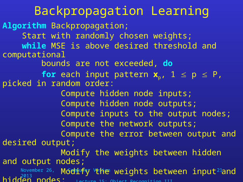
Backpropagation LearningAlgorithm Backpropagation; Start with randomly chosen weights; while MSE is above desired threshold and computational bounds are not exceeded, do for each input pattern xp, 1 p P, picked in random order: Compute hidden node inputs; Compute hidden node outputs; Compute inputs to the output nodes; Compute the network outputs; Compute the error between output and desired output; Modify the weights between hidden and output nodes; Modify the weights between input and hidden nodes; end-for end-while.
November 26, 2013 Computer Vision Lecture 15: Object Recognition III
22
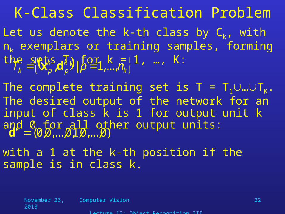
K-Class Classification ProblemLet us denote the k-th class by Ck, with nk exemplars or training samples, forming the sets Tk for k = 1, …, K:
kkp
kpk npT ,...,1|, dx
The complete training set is T = T1…TK.The desired output of the network for an input of class k is 1 for output unit k and 0 for all other output units:
)0,...,0,1,0,...,0,0(kd
with a 1 at the k-th position if the sample is in class k.
November 26, 2013 Computer Vision Lecture 15: Object Recognition III
23
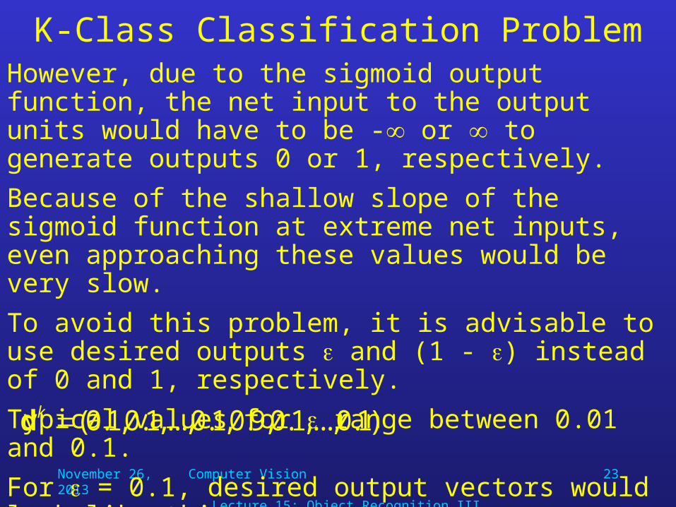
K-Class Classification ProblemHowever, due to the sigmoid output function, the net input to the output units would have to be - or to generate outputs 0 or 1, respectively.
Because of the shallow slope of the sigmoid function at extreme net inputs, even approaching these values would be very slow.
To avoid this problem, it is advisable to use desired outputs and (1 - ) instead of 0 and 1, respectively.
Typical values for range between 0.01 and 0.1.
For = 0.1, desired output vectors would look like this:
)1.0,...,1.0,9.0,1.0,...,1.0,1.0(kd
November 26, 2013 Computer Vision Lecture 15: Object Recognition III
24
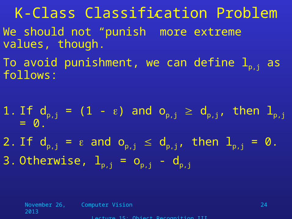
K-Class Classification ProblemWe should not “punish” more extreme values, though.
To avoid punishment, we can define lp,j as follows:
1. If dp,j = (1 - ) and op,j dp,j, then lp,j = 0.
2. If dp,j = and op,j dp,j, then lp,j = 0.
3. Otherwise, lp,j = op,j - dp,j
November 26, 2013 Computer Vision Lecture 15: Object Recognition III
25
NN Application Design
Now that we got some insight into the theory of backpropagation networks, how can we design networks for particular applications?
Designing NNs is basically an engineering task.
For example, there is no formula that would allow you to determine the optimal number of hidden units in a BPN for a given task.
November 26, 2013 Computer Vision Lecture 15: Object Recognition III
26
Training and Performance Evaluation
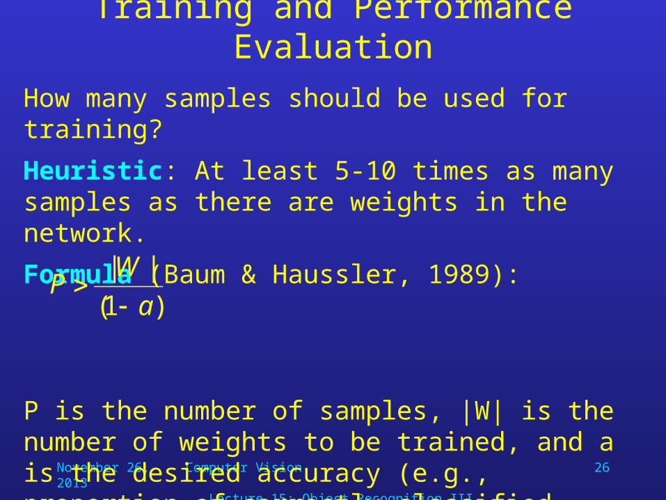
How many samples should be used for training?
Heuristic: At least 5-10 times as many samples as there are weights in the network.
Formula (Baum & Haussler, 1989):
P is the number of samples, |W| is the number of weights to be trained, and a is the desired accuracy (e.g., proportion of correctly classified samples).
)1(
||
a
WP
November 26, 2013 Computer Vision Lecture 15: Object Recognition III
27
Training and Performance EvaluationWhat learning rate should we choose?
The problems that arise when is too small or to big are similar to the perceptron.
Unfortunately, the optimal value of entirely depends on the application.
Values between 0.1 and 0.9 are typical for most applications.
Often, is initially set to a large value and is decreased during the learning process.
Leads to better convergence of learning, also decreases likelihood of “getting stuck” in local error minimum at early learning stage.
November 26, 2013 Computer Vision Lecture 15: Object Recognition III
28
Training and Performance Evaluation
When training a BPN, what is the acceptable error, i.e., when do we stop the training?
The minimum error that can be achieved does not only depend on the network parameters, but also on the specific training set.
Thus, for some applications the minimum error will be higher than for others.
November 26, 2013 Computer Vision Lecture 15: Object Recognition III
29
Training and Performance Evaluation
An insightful way of performance evaluation is partial-set training.
The idea is to split the available data into two sets – the training set and the test set.
The network’s performance on the second set indicates how well the network has actually learned the desired mapping.
We should expect the network to interpolate, but not extrapolate.
Therefore, this test also evaluates our choice of training samples.

November 26, 2013 Computer Vision Lecture 15: Object Recognition III
30
Training and Performance Evaluation
If the test set only contains one exemplar, this type of training is called “hold-one-out” training.
It is to be performed sequentially for every individual exemplar.
This, of course, is a very time-consuming process.
For example, if we have 1,000 exemplars and want to perform 100 epochs of training, this procedure involves 1,000999100 = 99,900,000 training steps.
Partial-set training with a 700-300 split would only require 70,000 training steps.
On the positive side, the advantage of hold-one-out training is that all available exemplars (except one) are use for training, which might lead to better network performance.
November 26, 2013 Computer Vision Lecture 15: Object Recognition III
31
Example: Face Recognition
Now let us assume that we want to build a network for a computer vision application.
More specifically, our network is supposed to recognize faces and face poses.
This is an example that has actually been implemented.
All information, such as program code and data, can be found at:http://www-2.cs.cmu.edu/afs/cs.cmu.edu/user/mitchell/ftp/faces.html
November 26, 2013 Computer Vision Lecture 15: Object Recognition III
32
Example: Face Recognition
The goal is to classify camera images of faces of various people in various poses.
Images of 20 different people were collected, with up to 32 images per person.
The following variables were introduced:• expression (happy, sad, angry, neutral)• direction of looking (left, right, straight ahead, up)• sunglasses (yes or no)
In total, 624 grayscale images were collected, each with a resolution of 30 by 32 pixels and intensity values between 0 and 255.
November 26, 2013 Computer Vision Lecture 15: Object Recognition III
33
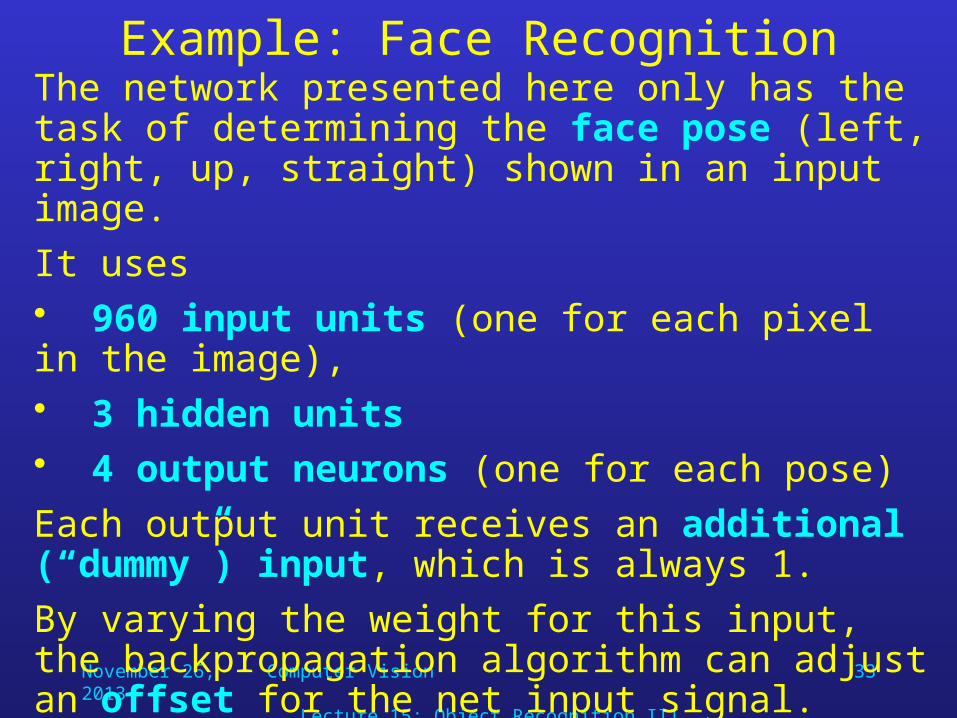
Example: Face RecognitionThe network presented here only has the task of determining the face pose (left, right, up, straight) shown in an input image.
It uses • 960 input units (one for each pixel in the image),• 3 hidden units • 4 output neurons (one for each pose)
Each output unit receives an additional (“dummy”) input, which is always 1.
By varying the weight for this input, the backpropagation algorithm can adjust an offset for the net input signal.
November 26, 2013 Computer Vision Lecture 15: Object Recognition III
34
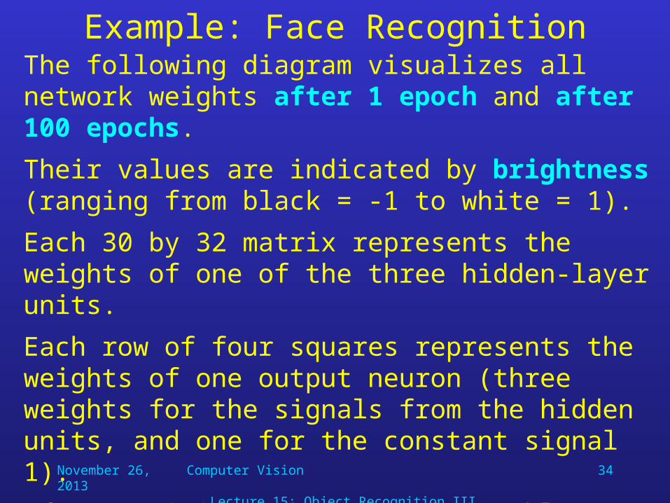
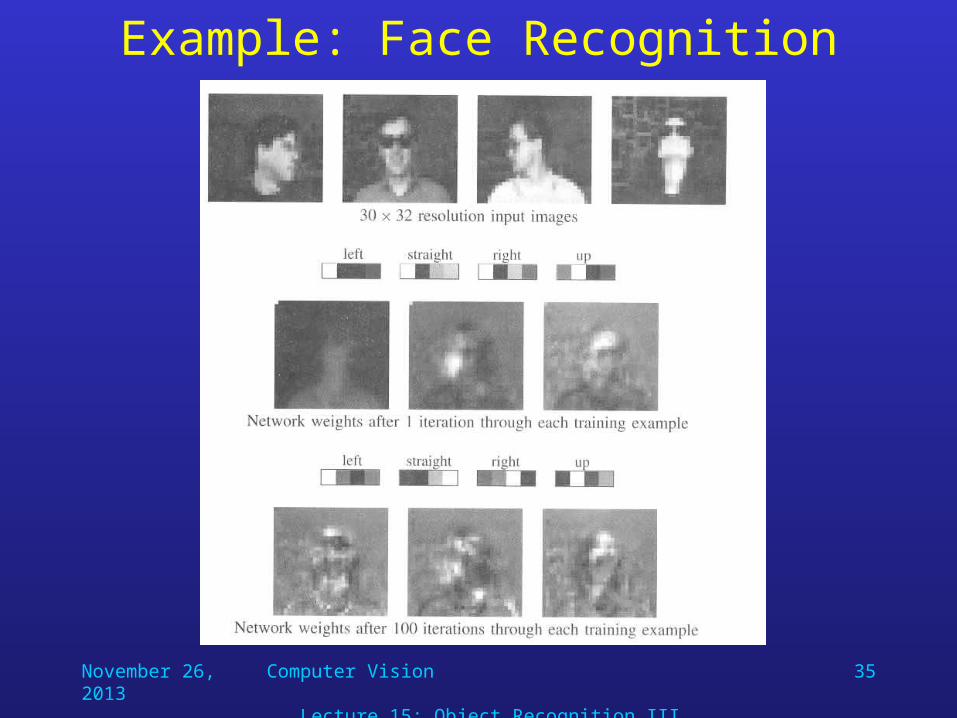
Example: Face RecognitionThe following diagram visualizes all network weights after 1 epoch and after 100 epochs.
Their values are indicated by brightness (ranging from black = -1 to white = 1).
Each 30 by 32 matrix represents the weights of one of the three hidden-layer units.
Each row of four squares represents the weights of one output neuron (three weights for the signals from the hidden units, and one for the constant signal 1).
After training, the network is able to classify 90% of new (non-trained) face images correctly.
November 26, 2013 Computer Vision Lecture 15: Object Recognition III
35
Example: Face Recognition
November 26, 2013 Computer Vision Lecture 15: Object Recognition III
36
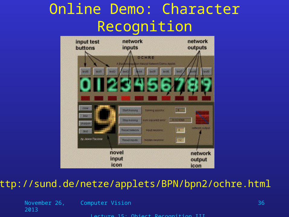
Online Demo: Character Recognition
http://sund.de/netze/applets/BPN/bpn2/ochre.html