Background Paper 2003:5 - AgEcon Searchageconsearch.umn.edu/bitstream/15606/1/bp030005.pdf ·...

Background Paper Series

Background Paper 2003:5

Functional forms used in CGE models: Modelling production

and commodity flows

Elsenburg August 2003

Overview

The Provincial Decision-Making Enabling (PROVIDE) Project aims to facilitate policy design by supplying policymakers with provincial and national level quantitative policy

information. The project entails the development of a series of databases (in the format of Social Accounting Matrices) for use in Computable General Equilibrium

models.

The National and Provincial Departments of Agriculture are the stakeholders and funders of the PROVIDE Project. The research team is located at Elsenburg in the

Western Cape.

PROVIDE Research Team

Project Leader: Cecilia Punt Senior Researchers: Kalie Pauw Melt van Schoor Junior Researchers: Benedict Gilimani Lillian Rantho Technical Expert: Scott McDonald Associate Researchers: Lindsay Chant Christine Valente

PROVIDE Contact Details

Private Bag X1 Elsenburg, 7607 South Africa

[email protected] +27-21-8085191 +27-21-8085210

For the original project proposal and a more detailed description of the project,

please visit www.elsenburg.com/provide

PROVIDE Project Background Paper 2003:5 August 2003

i © PROVIDE Project

Functional forms used in CGE models: Modelling production and

commodity flows1

Abstract

Various well-known functional forms, such as the Cobb-Douglas function, the Leontief function and the Constant Elasticity of Substitution (CES) function, are used frequently in economic modelling. Traditionally these functional forms have been used to model the production side (isoquants) or consumption side (indifference curves) of microeconomic models. The standard approach in CGE modelling has been to adapt the single-level value-added type production structure to a multi-level production structure, thereby including value-added as well as intermediate inputs. This is typically referred to as ‘nested’ production structures, and often makes use of combinations of Cobb-Douglas/CES and Leontief functions. In open-economy CGE models CES functions and the related Constant Elasticity of Transformation (CET) functions have been used to model consumers’ and producers’ decision-making process regarding consumption of production of traded goods (imports or exports) and domestic goods. The various applications of these functional forms are discussed in this paper, with a specific focus on the production side and commodity flows.

1 The main author of this paper is Kalie Pauw, Senior Researcher of the PROVIDE Project. This version was

revised in December 2004.


ii © PROVIDE Project

Table of Contents

1. Introduction .................................................................................................................1 1.1. Linear homogeneity and Euler’s Theorem............................................................1 1.2. Elasticity of substitution and transformation (EOS/EOT) ....................................4

2. Functional forms used to model production.............................................................6 2.1. The Cobb-Douglas function ..................................................................................6 2.2. The CES function ..................................................................................................9

3. Application in CGE models......................................................................................12 3.1. Basic model with no intermediate inputs ............................................................12 3.2. Introducing intermediate inputs - nested production structures..........................14

3.2.1. CES top-level function.................................................................................15 3.2.2. Leontief top-level function...........................................................................15 3.2.3. Second level value added and intermediate input functions .......................15 3.2.4. Simplification of the model structure ..........................................................16

4. Armington (CES/CET) functions – commodity flows in open economy models.17 5. Concluding remarks..................................................................................................20 6. Bibliography ..............................................................................................................21


iii © PROVIDE Project

List of Figures Figure 1: Three production functions and their associated EOS...............................................6 Figure 2: Price and quantity system for a closed 2*2*2*2 model with no intermediate inputs

.........................................................................................................................................13 Figure 3: Nested production structures ...................................................................................14 Figure 4: Price and quantity system for a closed 2*2*2*2 model with intermediate inputs ..17 Figure 5: A Basic 123 Model ..................................................................................................19 Figure 6: Flows of marketed commodities in the IFPRI standard model ...............................20


1

1. Introduction

Various functional forms can be used to model production and consumption in a CGE model. The most frequently used functional forms include the Cobb-Douglas function, the Leontief input-output function, and the Constant Elasticity of Substitution (CES) function. However, these functions are not only used to model consumption and production. CES functions and the related Constant Elasticity of Transformation (CET) functions have also been used as aggregation and transformation functions. Their application in open-economy models that incorporate international trade was an important development in the CGE literature. The incorporation of trade makes it necessary to model producers’ decisions about how they allocate production to the domestic and foreign markets (CET function). Similarly, consumers’ choices regarding the mix of imported versus domestically produced commodities should also be modelled (CES functions).

This note provides a theoretical background to the Cobb-Douglas function, the Leontief input-output function, and the CES function, and focuses particularly on their application in modelling production in a CGE model such as the Basic 2*2*2*2 and standard IFPRI/PROVIDE CGE models. Before looking at the functional forms and their characteristics in section 2, some important concepts are reviewed in sections 1.1 and 1.2. Section 3 looks at the application of these functions in the modelling of production in CGE models. Section 4 discusses the use of CES and CET functions in modelling trade flows.

1.1. Linear homogeneity and Euler’s Theorem

A function ( )nxxfy ,...,1= is said to be homogenous of degree r if multiplication of each of its independent variables by a positive constant λ changes the value of the function by a proportion λr (Chiang, 1984: 410). The degree of homogeneity can be determined by factoring out the term λr. Thus, the function ( )nxxfy ,...1= is said to be homogenous of degree r if

( ) ( )nr

n xxfxxf ,...,.,..., 11 λλλ = [1.1]

The degree of homogeneity is important in microeconomic production theory because it determines whether a function exhibits decreasing, constant or increasing returns to scale. A production function that is homogenous of degree one (or linearly homogenous) exhibits constant returns to scale. Thus, if all factors are doubled (say) outputs will also double. This can be verified for r = 1 and λ = 2 in equation 1.1.


2

A further important feature of linearly homogenous functions is that they satisfy Euler’s Theorem. For a linearly homogenous function ),...,( 1 nxxfy = Euler’s Theorem will yield the following identity:

∑=

≡n

iii yfx

1

where i

n

ii x

xxfxyf

∂∂

=∂∂

=),...,( 1 [1.2]

A basic proof is provided here.2 By definition homogeneity of degree one implies that ).()(. xfxf λλ = where x denotes an n-dimensional vector ),...,( 1 nxxx = and λ is a scalar.

Differentiating both sides with respect to xi and using the chain rule, we see that:

i

i

ii xx

xxf

xxf

xfxf

∂∂

∂∂

=∂

∂∂

∂ ).().().()(

)()(. λ

λλλ [1.3]

Since λλ =∂∂ )()(. xfxf and λλ =∂∂ ii xx ).( the equation above becomes

).().()(

ii xxf

xxf

λλ

∂∂

=∂

∂ [1.4]

Now, both sides of the original expression ).()(. xfxf λλ = are differentiated with respect to λ, yielding the following:

λλ

λλ

λλ

∂∂

∂∂

=∂

∂ ∑=

).().().()(.

1

in

i i

xxxfxf [1.5]

Since )()(. xfxf =∂∂ λλ and ii xx =∂∂ λλ ).( for all i = 1,…,n the expression above reduces to:

∑= ∂

∂=

n

i ii x

xfxxf1 ).(

).()(λλ [1.6]

Using the equality in equation 1.4 we can substitute ixxf ∂∂ )( for ).().( ixxf λλ ∂∂ , thus proving that Euler’s Theorem holds (equation 1.2). A corollary to Euler’s Theorem is that the first order derivatives )(xfi (i = 1,…,n) of the linearly homogenous function )(xf are homogenous of degree zero.3 The implication of this for CGE models is important in the understanding of how CGE models work. Many of the price equations in a CGE model are

2 See http://cepa.newschool.edu/het/essays/math/euler.htm. An alternative proof is provided in Chiang (1984:

412-414) for a production function of the form ( )LKfQ ,= in two inputs. Chiang’s proof can, with some difficulty, be extended to the case of n independent variables (inputs). The proof here proves Euler’s Theorem directly for the n-input case.

3 In general if the function )(xf is homogenous of degree k the first derivatives )(xfi are themselves homogenous of degree k-1. A proof for this corollary is not provided here (see footnote 2 for a reference).


3

first order differentials of the quantity equations that are linearly homogenous.4 Thus, CGE models are typically homogenous of degree zero in prices. A doubling of all prices will have no impact on quantities. Despite the restrictions that linear homogeneity imposes on production functions, they are frequently used due to this and various other “nice mathematical properties” (Chiang, 1984: 414) that they possess.

A further important implication of Euler’s Theorem is the product exhaustion theorem (see Chiang, 1984: 414). If the production function is linearly homogenous, i.e. exhibits constant returns to scale, and each factor (F) is paid a wage (WF) equal to the value of that factor’s marginal revenue product (MRPF), the shares (of output) paid to the factors will exhaust the value of total output. To show this result, consider a production function

( )nxxfQ ,...,1= where the xi’s represent the n factors of production and Q the output. The MRPF of a factor is defined as the marginal physical product (MPPF) of that factor multiplied by the price of the goods produced by the factor:

PMPPMRP FF .= where F

F xQMPP

∂∂

= [1.7]

Under conditions of perfect competition the employer will hire additional units of a factor as long the additional factor cost (wage) is less than the additional revenue generated by that factor. The firm will continue to do so until FF MRPW = for all factors. Suppose the production function in two inputs ( )LKfQ ,= is linearly homogenous. Applying Euler’s Theorem yields

LK MPPLMPPKLQL

KQKQ

.. +=∂∂

+∂∂

≡ [1.8]

The MPPF in each term on the right-hand side of equation 1.8 can now be replaced by the expression in equation 1.7. Thus, when FF MRPW = in equilibrium (profit-maximising condition), the following holds:

LK

LK

WLWKQPP

MRPL

PMRP

KQ

... +=∴

+≡ [1.9]

This result shows that the shares of total product paid to the factors capital and labour respectively, i.e. the wage times the employment level, exhaust the total product if WF equals

4 Some of the price equations are accounting definitions.


4

the MRPF. It only applies in the long run (equilibrium) and under conditions of perfectly competitive product and factor markets, i.e. zero economic profits are made.5

1.2. Elasticity of substitution and transformation (EOS/EOT)

The EOS and the EOT, denoted by σ and Ω respectively, determine the degree of substitutability or ‘transformability’ between inputs. Consider a standard convex production function in two inputs ),( LKfQ = . For a given isoquant representing some constant level of output, say Q , the firm can substitute labour for capital, thus moving along the isoquant without sacrificing or gaining output. The marginal rate of technical substitution of labour for capital (MRTSLK) is defined as dLdK− . It shows the rate at which labour can be substituted for capital while holding output constant (i.e. along the isoquant). In equilibrium the MRTSLK is equal to the ratio of prices (factor costs), (WL/WK). Any rational profit-maximising firm will alter its capital-labour ratio in response to a change in the price ratio. The EOS measures the proportionate change in the capital-labour ratio (K/L) relative to a proportionate change in the ratio of prices ( LKKL MRTSWW = ) (Nicholson, 1992: 308). Thus,

( ) ( )( ) ( )LK

MRTSMRTSd

LKdMRTS

LK LK

LKLK //

%/%

=∆∆

=σ [1.10]

Note that the capital-labour ratio declines as labour is substituted for capital, i.e. labour is increased and capital is decreased. At the same time the slope of the isoquant (MRTSLK) also declines, provided the production function is convex with respect to the origin. The EOS is thus a ratio of the rate of decline of the capital-labour ratio and the rate of decline of the MRTSLK. Most mathematical production and consumption functions used in economics are set-up in such a way that the EOS is constant, i.e. the rate of decline of the capital-labour ratio is equal to the rate of decline of the slope of the isoquant as labour is substituted for capital.6 Note that the EOT refers to the same concept relating to transformation functions, i.e. functions that are concave with respect to the origin.

5 This result can easily be extended to production functions in multiple inputs. For the linearly homogenous

production function ( )nxxfQ ,...,1= Euler’s Theorem yields the following identity:

∑=

=

+++≡n

iii

nn

MPPx

MPPxMPPxMPPxQ

1

2211 ... [1.8a]

Substituting the expression for MPPi yields

∑∑

∑

==

=

==∴

≡

n

iii

n

iii

n

i

ii

WxMRPxQP

PMRPxQ

11

1

.

[1.9a]

6 The EOS along a consumer’s indifference curve can be calculated in the same fashion.


5

Below three functional forms are considered, each with different (constant) elasticities of substitution. The same principle applies throughout to concave functions and the EOT. It is shown that the larger the value of σ, the easier factors can be substituted. The comparison presented here should illustrate clearly that the EOS is effectively a measure of the curvature of an isoquant.

Firstly, consider a linear isoquant of the form LbKaQ .. += , which is characterised by perfect substitutability between the factors. For a given level of output Q the absolute value of the slope of this function is given by LKMRTSabdLdK == . Since the slope is constant for all possible combinations of K and L, the change in the MRTSLK will always be zero. Consequently σ is undefined or “infinite” due to division by zero. Thus, for linear production functions characterised by perfect substitutability between factors, the EOS is infinite.

At the other extreme the Leontief input-output function is characterised by zero substitutability because inputs are used in fixed proportions to the level of output. Any profit-maximising firm will always produce at the corner point of this L-shaped function. Thus, as the ratio of factor prices change, the capital-labour ratio will remain unchanged. The percentage change in the capital-labour ratio is therefore always zero along a given Leontief input-output isoquant, and as a consequence the EOS is also zero for functions with zero substitutability between factors.

The linear and Leontief production functions represent the two extremes for convex production functions, and hence the upper and lower boundaries of the EOS are defined by the expression 0 ≤ σ ≤ ∞. Next we consider the Cobb-Douglas function, which is characterised by imperfect substitutability. The expectation is that the EOS should be somewhere between these two extremities. In fact, the EOS of a standard Cobb-Douglas function is one (1) (see worked example below). Figure 1 below shows these results graphically.


6

Figure 1: Three production functions and their associated EOS

K KK

L L Lσ = ∞ σ = 0σ = 1

Linear production function Cobb-Douglas function Leontief function

The EOS of any linearly homogenous production of the form ),( LKfQ = can be calculated using a formula derived by Allen (see Nicholson, 1992: 309):

KLQQKQLQ

∂∂∂∂∂∂∂

= 2.*σ [1.11]

This formula can be used to calculate the EOS of the linearly homogenous Cobb-Douglas function, αα −= 1. LKAQ . It is fairly easy to see that σ = 1 and constant at any point along the isoquant.

[ ] [ ][ ]

1..)1(

..)1(

1

1

11

==

−

−=

−

−−

−−−

QLKA

LKAQ

LKALKA

αα

αα

αααα

αα

αασ

[1.12]

The calculation of the EOS for a production function in more than two inputs “raises several complications” (Nicholson, 1992: 309). In the real world a change in the ratio of two inputs is likely to have an effect on the level of other inputs as well due to interdependencies between various factors. Most factors are complements or substitutes of each other, but these relationships are not necessarily stable when changing different combinations of factors.

2. Functional forms used to model production

2.1. The Cobb-Douglas function

The Cobb-Douglas function is without doubt the most widely used function in general economics (Heathfield and Wibe, 1987: 76). It owes part of its name to Paul Douglas who


7

used US manufacturing data for the period 1899 - 1922 to infer its properties. His colleague Cobb, a mathematician, suggested the functional form. Although the function was initially based on manufacturing data and two inputs (capital stock and labour), it can be extended to include multiple inputs. It can also be used to model consumption (utility functions). The two-input Cobb-Douglas production function has the following form:

βα LKAQ .= [2.1]

The parameter A (A > 0) is known as a shift or efficiency parameter. The parameters α and β (0 ≤ α ≤ ∞, 0 ≤ β ≤ ∞) are the function exponents. The function exponents determine the degree of homogeneity. If each factor is increased by a factor λ total output will increase by λα+β.

QLKALKAQ βαβαβαβα λλλλ ++ ===′ .).().( [2.2]

The Cobb-Douglas function will exhibit constant returns to scale if the function exponents are restricted to sum to unity. If α + β = 1, β can be replaced by the expression β = 1 - α, and hence we can rewrite the Cobb-Douglas function as αα −= 1. LKAQ . To illustrate an important characteristic of the Cobb-Douglas function, the MPP of each factor is calculated below:

ααα αα =⇒== −−

QMPPK

KQLKMPP K

K..11 [2.3a]

)1(..)1( ααα αα −=⇒=−= −

QMPPL

LQLKMPP L

L [2.3b]

The result in 2.3 shows that, for a linearly homogenous Cobb-Douglas function, the function exponent of each factor represents the relative share (contribution) of that factor in total output. Furthermore, if each factor is paid the value of its MPP, i.e. WF = MRPF = MPPF.P, the equilibrium wage will be a fixed share of the average revenue product (ARPF) of that factor, where the ARPF is defined as the average product ( FQAPF = ) multiplied by price P:

KKK ARP

KQPW

QPMRPK

....

.ααα ==⇒= [2.4a]

LLL ARP

LQPW

QPMRPL

)1(.)1()1(.

.ααα −=

−=⇒−= [2.4b]

The equations in 2.4 are typically used as the first order conditions for profit maximisation, also known as the factor demand equations. The result can also be obtained by directly applying Euler’s Theorem (equation 1.9). The factor demand equations satisfy the


8

optimal input-ratio, which is derived using the standard approach to profit maximisation. Consider the linearly homogenous Cobb-Douglas function αα −= 1. LKAQ in two inputs. If the firm wishes to maximise profits a profit function (Π) needs to be defined as the total revenue (TR) minus total cost (TC); thus:

LWKWLKAP

LWKWQPTCTR

LK

LK

−−=

−−=−=Π

−αα 1..

. [2.5]

Differentiation with respect to K and L gives the following two equations, both of which should be simultaneously set equal to zero:

0... 11 =−=∂Π∂ −−

KWLKAPK

ααα [2.6]

( ) 0..1 =−−=∂Π∂ −

LWLKAPL

ααα [2.7]

This gives the optimal ratio of employment in equilibrium. It can be verified that the result obtained in equation 2.4 satisfies this equilibrium condition:

αα−

=1K

L

WW

LK [2.8]

Next, factor demand equations for K and L can be derived by substituting the above expression into the Cobb-Douglas production function. This will yield factor demand equations of the form ( )*,, QWWKK LK= and ( )*,, QWWLL LK= , where Q* is the profit-maximising level of output. The problem with this approach is that the derivation of the factor demand equations becomes complicated when dealing with functions in more than two inputs, since first order condition equations need to be solved simultaneously for every factor. As a result the “Euler approach” is preferred when dealing with multiple-input Cobb-Douglas production functions.

The n-input Cobb-Douglas function will take on the following form:

∏=

=

=n

ii

n

i

n

xA

xxxAQ

1

21 .... 21

α

ααα

[2.9]

The first-order condition for profit maximisation for this function is derived below. As before (see equation 2.2) multiplication of each factor xF by a factor λ will cause output to increase by a factor nααλ ++...1 . Thus, if 1...1 =++ nαα , the function is linearly homogenous.


9

The parameter αF represents, as before, the share of total product accruing to each factor, as is shown for factor F below:

FnFknFFFFF

QxxxA

QxxxAx

QMPPx nFnF

ααα αααααα

===− .............. 11

11

1 [2.10]

Since FF MPPPMRP .= and FF MRPW = in equilibrium the following equilibrium condition can be derived (the first-order condition for profit maximisation):7

F

FF x

QPW

.α= [2.11]

2.2. The CES function

Although widely used, the Cobb-Douglas function has one large drawback: the EOS always takes on a value of one (see section 1.2). The CES function, first developed by Arrow, Chenery, Minhas and Solow (see Nicholson, 1992: 313), allows for greater flexibility in that the modeller can choose the value of the EOS. This function takes on the following form in the two-input case:

[ ] ρε

ρρ δδ−

−− −+= LKAQ )1( [2.12]

The parameter A (A > 0) is, as in the Cobb-Douglas function, an efficiency or shift parameter. The parameter δ (0 ≤ δ ≤ 1) is a distribution or share parameter. It permits the relative importance of the inputs to vary, thus operating in much the same way as the function exponents of the Cobb-Douglas production function. The parameter ρ (-1 ≤ ρ ≤ ∞, ρ ≠ 0) is the substitution parameter or function exponent. The relationship between this parameter and the EOS is explained below. Finally, ε (0 ≤ ε ≤ ∞) determines the degree of homogeneity of the function. The function can exhibit increasing, decreasing or constant returns to scale,

7 The commodity demand equations for consumers are similar. Consider a Cobb-Douglas utility function

αα −= 121 xxU . Suppose the consumer wishes to maximise utility subject to a budget constraint

2211 xPxPY += , where Y is the consumer’s income, and P1 and P2 are the prices of commodities x1 and x2 respectively. Solving the resulting Lagrangian function yields consumer demand equations:

11 P

Yx α= and

22

)1(P

Yx α−=

Thus, consumers allocate fixed proportions of their income to each commodity. In a Cobb-Douglas utility function in n commodities, n

nxxU αα ...11= will yield the following utility maximising commodity demand

equation for commodity C:

C

CC P

Yx

α=


10

depending on the value of ε. Multiplying each factor by a constant λ changes the level of output as follows:

[ ]

[ ]Q

LKA

LKAQ

.)1(..

).)(1().(

ε

ρρε

ρρ

λ

δδλ

λδλδ

ρε

ρε

=

−+=

−+=′−

−

−−

−−

[2.13]

Thus, if ε < 1, the function exhibits decreasing returns to scale, if ε = 1 there are constant returns to scale and if ε > 1 there are increasing returns to scale. For reasons discussed before only linearly homogenous production functions are used in CGE models. Using the formula in equation 1.11 the relationship between the EOS of a linearly homogenous CES function and the function exponent can be shown to be the following: 8

ρσ

+=

11 , 0 ≤ σ ≤ ∞ [2.14]

The range of the function exponent was given as -1 ≤ ρ ≤ ∞, ρ ≠ 0. The CES function is not defined for ρ = 0 due to division by zero. However, using L’Hôpital’s Rule it can be shown that as ρ → 0, the linearly homogenous CES production function approaches the linearly homogenous Cobb-Douglas function (see Chiang, 1984: 429-430). In a way the CES encompasses all of the functional forms shown in Figure 1, i.e. the linear production function, Cobb-Douglas production function and Leontief production function can be regarded as special cases of the generliased CES function. The flexibility of the CES function has contributed to its popularity in CGE modelling.

The first-order condition for profit-maximisation can be derived directly by substituting the profit maximising condition (WF = MRPF) into the equation for the MPPF:

[ ] [ ]

[ ] [ ]1

1

.)1(.

)()1(.1

11

11

−−−−

−−−−

−−

−−

−+=

−−+

−=

ρρρ

ρρρ

δδδ

ρδδδρ

ρ

ρ

KLKAP

MRP

KLKAMPP

K

K

[2.15]

[ ] [ ]1.)1(..1

1

−−−−−−

−+=∴ ρρρ δδδρ

KLKAPWK [2.16]

8 Some textbooks formulate the CES function as [ ]ρε

ρρ δδ LKAQ )1(. −+= and then define the range of the function exponent as (-∞ ≤ ρ ≤ 1, ρ ≠ 0). This will cause equation 2.14 to change to ( )ρσ −= 11 , with the range of the EOS remaining the same. The formulation in equation 2.12 will be used throughout this paper.


11

The equilibrium factor demand equation for L can be derived in similar fashion.

[ ] [ ]1)1()1(..1

1

−−−− −−+=∴−−

ρρρ δδδρ

LLKAPWL [2.17]

It is easy to show that these equations satisfy the first-order condition for profit maximisation that can be derived by defining a profit function (Π) as TR minus TC:

[ ] LWKWLKAP LK −−−+=Π−

−−ρ

ρρ δδ1

)1(.. [2.18]

Taking the first order partial differentials of the profit function with respect to K and L respectively and solving these simultaneously yields the following profit equilibrium condition:

L

K

WW

KL

=

−

+1

1

ρ

δδ [2.19]

The CES function is easily extended to include multiple inputs. The generalised multiple-input CES function ( )nxxfQ ,...,1= takes on the following form:

[ ]ρε

ρ

ρε

ρρρ

δ

δδδ−

=

−

−−−−

=

+++=

∑n

iii

nn

xA

xxxAQ

1

2211 ... [2.20]

As before (see equation 2.13) multiplication of each of the factor xF by a factor λ will increase output by a factor λε. Thus, this function will be linearly homogenous for ε = 1. The first order condition for profit maximisation looks similar those derived for the two-input function (equations 2.16 and 2.17): 9

[ ] [ ]

[ ]111

1

111

2211

.

....

−−−−

=

−

−−−−−−−

=

+++=

∑ ρρρ

ρρρρρ

δδ

δδδδ

FxP

FxxxAPW

F

n

iii

FnnF

[2.21]

Related to the CES function is the Constant Elasticity of Transformation (CET) function. A CET function has a similar functional form, but is concave with respect to the origin (in the

9 CES functions are seldom used to model consumer utility. The Cobb-Douglas function is more suited for this

since the abstract concept of “utility” can be avoided by assuming that consumers allocate a fixed proportion of their disposable income to each commodity. The CES function does not have this characteristic – in fact, this was exactly the reason why the CES function was developed – and consequently “utility” enters as a variable in the first-order conditions for utility maximisation.


12

two-dimensional case). The only difference in the mathematical statement is that the negative sign in front of the function exponent disappears. The range of the function exponent remains (-1 ≤ ρ ≤ ∞, ρ ≠ 0). Section 4 provides an example of how the CET function may be used in a CGE model with international trade.

3. Application in CGE models

3.1. Basic model with no intermediate inputs

In the basic model with no intermediate inputs production is modelled as a simple value-added type Cobb-Douglas function (see Löfgren, 1999: 4-10). Thus, the output of each activity (QXa) is a function of the primary inputs or factors of production (FDf,a). Note that the function is indexed over activities a (compare equations 2.1 and 2.9):10

∏∈

=Ff

afxaa

afFDadQX ,,

α [3.1]

The values of the αf,a’s are restricted to sum to unity, and hence we can use Euler’s Theorem to derive the first order condition for profit maximisation, or the factor demand equation. This function is indexed over factors f (compare equation 2.11):

af

aaaff FD

QXPXWF

,

,α= [3.2]

Alternatively a CES production function may be used. This function appears below (compare equation 2.21):

xa

xa

faf

xaf

xaa FDadQX

ρρδ

/1

,,

−

−

= ∑ [3.3]

The first-order condition for profit maximisation can either be calculated by differentiating the profit function with respect to each factor. Alternatively, the MPPF can be calculated directly by differentiating QXa with respect to FDf,a.

[ ]1,

11

,,

,,

−−

−−

−

=

∂∂ ∑

xa

af

xax

a

afa afx

faf

xx

af

a FDFDadFDQX ρ

ρρ δδ [3.4]

As before, the MPPF can be replaced by the expression af PXWF , the condition for profit maximisation. Thus,

10 Notation used here complies as far as possible with the PROVIDE Project CGE model notation rather than

that used by Löfgren (see PROVIDE, 2003).


13

[ ]1,

11

, ,,

−−

−−

−

= ∑

xa

af

xax

aafa af

x

faf

xxaf FDFDadPXWF ρ

ρρ δδ [3.5a]

OR

[ ]1,

1

, ,,

−−

−

−

= ∑

xa

af

xa

afa afx

faf

xxaaf FDFDadQXPXWF ρρ δδ [3.5b]

The first formulation of the factor demand equation in 3.5a is similar to the equation derived in 2.21. In equation 3.5b QXa is factored out. Mathematically these two formulations are identical. However, the formulation selected depends on the closure rules of the model. Equation 3.5a should be used when the profit maximising level of output QXa and the levels of factor demand FDf,a are determined simultaneously. However, if a closure rule is selected whereby QXa is fixed, equation 3.5b should be used.

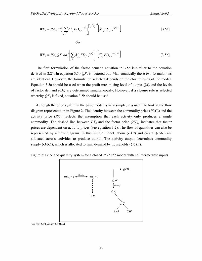
Although the price system in the basic model is very simple, it is useful to look at the flow diagram representation in Figure 2. The identity between the commodity price (PXCc) and the activity price (PXa) reflects the assumption that each activity only produces a single commodity. The dashed line between PXa and the factor price (WFf) indicates that factor prices are dependent on activity prices (see equation 3.2). The flow of quantities can also be represented by a flow diagram. In this simple model labour (LAB) and capital (CAP) are allocated across activities to produce output. The activity output determines commodity supply (QXCc), which is allocated to final demand by households (QCDc).

Figure 2: Price and quantity system for a closed 2*2*2*2 model with no intermediate inputs

PXCc = 1 PXa = 1

WFf

FDf,a

LAB CAP

QXa

QXCc

QCDc

identity

identity

Source: McDonald (2002a)


14

3.2. Introducing intermediate inputs - nested production structures

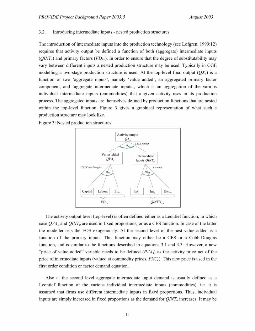
The introduction of intermediate inputs into the production technology (see Löfgren, 1999:12) requires that activity output be defined a function of both (aggregate) intermediate inputs (QINTa) and primary factors (FDf,a). In order to ensure that the degree of substitutability may vary between different inputs a nested production structure may be used. Typically in CGE modelling a two-stage production structure is used. At the top-level final output (QXa) is a function of two ‘aggregate inputs’, namely ‘value added’, an aggregated primary factor component, and ‘aggregate intermediate inputs’, which is an aggregation of the various individual intermediate inputs (commodities) that a given activity uses in its production process. The aggregated inputs are themselves defined by production functions that are nested within the top-level function. Figure 3 gives a graphical representation of what such a production structure may look like.

Figure 3: Nested production structures

Activity outputQXa

Value addedQVAa

IntermediateInputs QINTa

Capital Labour Int1 Int2

σqa

σva σint

Etc… Etc…

FDf,a QINTDc,a

CES/Leontief

LeontiefCES/Cobb-Douglas

The activity output level (top-level) is often defined either as a Leontief function, in which case QVAa and QINTa are used in fixed proportions, or as a CES function. In case of the latter the modeller sets the EOS exogenously. At the second level of the nest value added is a function of the primary inputs. This function may either be a CES or a Cobb-Douglas function, and is similar to the functions described in equations 3.1 and 3.3. However, a new “price of value added” variable needs to be defined (PVAa) as the activity price net of the price of intermediate inputs (valued at commodity prices, PXCc). This new price is used in the first order condition or factor demand equation.

Also at the second level aggregate intermediate input demand is usually defined as a Leontief function of the various individual intermediate inputs (commodities), i.e. it is assumed that firms use different intermediate inputs in fixed proportions. Thus, individual inputs are simply increased in fixed proportions as the demand for QINTa increases. It may be


15

necessary to define a new aggregate intermediate price variable (PINTa) if the top-level function is not a Leontief function. This will become clear in the discussion that follows. PINTa is essentially a weighted aggregation of the individual input prices (commodity prices). The model statement for two alternatives (CES or Leontief top-level) is discussed below, drawing on Löfgren et al. (2001), Löfgren (1999) and McDonald (2002a). The notation is similar to that used in the PROVIDE CGE model (see PROVIDE 2003).

3.2.1. CES top-level function

If the top-level production function is a CES function in two inputs, QVAa and QINTa the following equation is used

( ) xa

xa

xa

axaa

xa

xaa QINTQVAadQX ρρρ δδ

1

)1(−−− −+= [3.6]

The profit maximising input mix is derived by taking the first order differential of the profit equation (Π) with respect to the inputs. Thus,

aaaaaaa QINTPINTQVAPVAQXPX −−=Π [3.7]

This yields the following profit-maximising condition (compare equations 2.18 and 2.19):

xa

xa

xa

a

a

a

a

PVPINT

QINTQVA ρ

δδ +

−

=1

1

1 [3.8]

3.2.2. Leontief top-level function

If the top-level function is a Leontief function both inputs (QVAa and QINTa) are fixed proportions of activity output (QXa).

aaa QXivaQVA = and aaa QXintaQINT = [3.9]

3.2.3. Second level value added and intermediate input functions

The value added production function (QVAa) and its relevant factor demand equation is similar to equations 3.1/3.2 and 3.3/3.5 for the Cobb-Douglas and CES formulations respectively. The only difference is that value added is valued at the price PVAa rather than PXa, while QVAa replaces QXa. Thus, the Cobb-Douglas production function and is related factor demand equation is given by 3.10 and 3.11 respectively:

∏∈

=Ff

afvaaa

vaafFDadQVA ,

,α [3.10]


16

af

aava

aff FD

QVAPVWF

,

,α= [3.11]

Similarly, the CES value added function and its related factor demand equation (two alternatives) are given below (3.12 and 3.13):

vaa

vaa

faf

vaaf

vaaa FDadQVA

ρρδ

/1

,,

−

−

= ∑ [3.12]

[ ]1,,

11

,,−−

−−

−

= ∑

vaa

vaava

aaf

vaaf

faf

vaaf

vaaaf FDFDadPVWF ρ

ρρ δδ [3.13a]

OR

[ ]1,,

1

,,−−

−

−

= ∑

vaa

vaa

afva

aff

afva

afvaaaaf FDFDadQVAPVWF ρρ δδ [3.13b]

The second-level Leontief aggregation function combines intermediate inputs (defined over c) in fixed proportions to form aggregate intermediate inputs (defined over a):

aAa

acc QINTcomactcoQINTD ∑∈

= , [3.14]

3.2.4. Simplification of the model structure

In the 2*2*2*2 model the top-level function is a Leontief function, while at the second level the value added function is a Cobb-Douglas function. Also at the second level aggregate intermediate inputs is a Leontief function of intermediate inputs. Thus, all the functions along the right-hand side “leg” of the nest are Leontief functions. When this is the case it is possible to “collapse” the entire leg. The individual intermediate inputs (QINTDc) are aggregated in fixed proportions and the aggregate intermediate inputs (QINTa) are then used in fixed proportions in the top-level function. This simply implies that QINTDc are used in fixed proportions in the production of QXa and therefore the aggregation equation (3.9, right-hand side) can be left out, thus jumping directly to the following:

∑∈

=Aa

aacc QXcomactcoQINTD , [3.15]

Equations 3.9 (left-hand side) and 3.10 give the top-level and second level formulations for QAa and QVAa respectively. From these two equations the top-level function can be written as


17

∏

∏

∈

∈

=

=

=

Ffafa

Ffaf

vaa

a

aa

a

vaaf

vaaf

FDad

FDadiva

QVAiva

QA

,

,

,*

,1

1

α

α [3.16]

where aaa ivaadad =* . Equations 3.15 and 3.16 thus represent the entire nested production structure of the 2*2*2*2 model with intermediate inputs of Exercise 2. The model statement is a simplification of the expanded structure represented by equations 3.9 (top-level Leontief activity output), 3.12 (value added Cobb-Douglas function) and 3.14 (Leontief aggregate intermediate inputs). The price and quantity system of the model is represented in Figure 4.

Figure 4: Price and quantity system for a closed 2*2*2*2 model with intermediate inputs

PXCc = 1 PXa = 1

FDf,a

LAB CAP

QXa

QXCc

QCDc

identity

identity

∑c

ccaPica

PVAaQINTa

Source: McDonald (2002a)

The price and quantity system is not much different from before, except that the inclusion of intermediate inputs has necessitated the construction of a value added price

∑−=c

cacaa PXicaPXPV , , i.e. the activity price net of the cost of intermediate inputs valued

at commodity (consumer) prices, weighted according to the relative share of each intermediate commodity in aggregate intermediates.

4. Armington (CES/CET) functions – commodity flows in open economy models

The preceding chapters highlighted the use of CES production functions (inter alia) in the modelling of production in CGE models. However, these functions’ use is not limited to the modelling of production (or consumption). CES and CET functions may also be used to


18

model the flow of commodities in the economy. Specifically, they are employed as aggregation and transformation functions in models that incorporate international trade flows.

When a closed economy model is expanded to include a foreign sector local consumers have a choice between imported and domestically produced goods, while local producers can choose whether they wish to export their production or supply it to the local markets. Invariably consumers choose a mix of imported and domestic goods, while producers often supply to both domestic and foreign markets. It is therefore necessary to make certain assumptions regarding the substitutability between imports/domestic goods (consumers) and exports/domestic goods (producers). The standard neoclassical trade model assumes that all goods are tradable and that all goods are perfect substitutes (see McDonald, 2002b). Under these assumptions domestic prices are ultimately determined by world prices. The Salter-Swan or Australian model relaxed the assumption that all goods are traded by introducing a dichotomy between ‘tradeables’ and ‘non-tradeables’. However, the problem of finding ‘corner solutions’ (denoting complete specialisation) or large fluctuations in relative prices still remained for traded goods. The so-called ‘Armington assumption’ provided the solution to this problem. Armington (1969) suggested the assumption that imports/domestic demand and exports/domestic supply are imperfect substitutes. Since then the CGE literature has “virtually without exception” adopted the Armington assumption (McDonald, 2002b: 1).

One of the simplest models that incorporate trade is the so-called 123-Model, which has one country, two production sectors (exports or domestic supply) and three goods (imported goods, exported goods and domestically produced goods).11 This model is useful to explain how CES and CET functions are used in the modelling of trade flows under the Armington assumption. Consider the four-quadrant diagram in Figure 5. All dimensions in this diagram are positive. The production possibility frontier (PPF) in the fourth quadrant (IV) is used to allocate domestic production (QX) to the export market (QE) or the domestic market (QDS) depending on the relative prices of these goods. This PPF or transformation curve is concave with respect to the origin and usually takes on the functional form of the CET function. Profit is maximised at the point of tangency where the slope of the PPF equals the price ratio.

The balance of trade can be represented by a 45o line through the origin (quadrant I) based on the assumption of that export prices (PE) and import prices (PM) are equal and that the balance of trade is zero. Similarly the transformation of domestic supply (QDS) to domestic demand (QDD) is a one-to-one mapping. The information in quadrants I, III and IV can now be used to construct a consumption possibility frontier (CPF), which is concave with respect to the origin (quadrant II). Consumers maximise utility and hence consume a composite good (QQ), which is a combination of imported goods (QM) and domestically produced goods

11 For simplicity reasons the notation used here does not include subscripts.


19

(QDD) at the tangency between the indifference curve (convex with respect to the origin) and the line that represents the price ratio of domestic goods (PDD) relative to imported goods (PM). The utility level is of course subject to the CPF, the ‘budget constraint’ of the consumers.

Figure 5: A Basic 123 Model

QM

QDD QE

Balance of trade

QDS

II I

IVIII

Domestic market

DS

E

PP

( )QDSQEGQX ,=

( )),QDDQMFQQ =

M

DD

PP

Source: McDonald (2002b)

A similar approach to this is adopted in most other open-economy CGE models, including the single country GTAP model (McDonald, 2003), the IFPRI standard CGE model (Löfgren et al, 2001) and the PROVIDE CGE model (PROVIDE, 2003). Figure 6 shows how the IFPRI model makes use of a variety of substitution mechanisms to model the flow of marketed commodities. A CES aggregation function is used to aggregate domestic production into a single commodity (QX) 12, which is then allocated to the domestic (QDS) and export (QE) markets via a constant elasticity of transformation (CET) function (the PPF). A CES aggregation function (the CPF) is used to create a composite commodity (QQ) made up of domestic sales (QDD) and imported goods (QM). The composite commodity represents total domestic supply. One of the macroeconomic constraints imposed in the model ensures that domestic supply equals domestic consumption (the sum of household and government consumption) plus investment demand and intermediate input demand.

12 Note that some CGE models allow for industries to produce more than one type of commodity. Thus, this

aggregation function simply adds up similar commodity types across all industries. If each industry only produces a single commodity (such as is the case in Exercises 1 and 2 in Löfgren (1999)), commodity output QXC can be directly mapped to activity output QX.


20

Figure 6: Flows of marketed commodities in the IFPRI standard model

Commodityoutput:

1st activityAggregate

outputCommodity

output:Nth activity

Aggregateexports

Domesticsales

Aggregateimports

Compositecommodity

CES CET

CES

Householdconsumption

+Governmentconsumption

+Investment

+Intermediate

use

Source: Löfgren et al. (2001)

The model statement of the CES aggregation function and CET transformation function is provided below. Commodity output QX is allocated to the export (QE) and domestic (QDS) markets according to the CET function below:

( ) ttt QDSQEatQX ρρρ γγ1

)1( −+= [4.1]

The optimal allocation depends on the ratio of export to domestic prices, given by the following first-order condition:

11

1 −

−=

t

PDSPE

QDSQE ρ

γγ [4.2]

Similarly, the CES aggregation function and its first order condition is given by equations 4.3 and 4.4 below:

( ) ccc QDDQMacQQ ρρρ δδ1

)1(−−− −+= [4.3]

c

PMPDD

QDDQM ρ

δδ +

−=

11

1 [4.4]

5. Concluding remarks

In order to draw informed conclusions of CGE model results it is imperative that a proper understanding of the functional forms used in CGE models to model production, consumption


21

and commodity flows, is developed. The basic principles discussed in this paper should be a good start to understand the more complex CGE models, most of which are built on the same principles as the ones discussed in this paper. This paper focused on production and commodity flows, explaining the use of various well-known functional forms used in CGE models.

Some important related topics that fell beyond the scope of this particular paper, but are useful to mention include, firstly, explorations of multiple-level nested production functions. This paper only discussed the two-stage production structure. A multiple-level structure would allow for greater flexibility in the setting of substitution elasticities, for example, if labour is further disaggregated into skilled and unskilled labour using a third level of aggregation functions. Secondly, the price system relationships of the simple models described here as well as the more complex models need to be explored in more detail. Thirdly, the current version of the paper focuses mainly on the production side. The consumption side is just as important and various demand systems, especially the Stone-Geary system and the ‘almost ideal demand system’ should be explored for a better understanding of how the CGE model operates. Finally, a functional form that was not discussed in this paper is the translog production function. This function is a single-level function that can be used to estimate a nested production technology. It is also easier to extend a translog function than adding further nests in a nested production technology. Thus, if more detail is required the translog function may be preferable.

6. Bibliography Chiang, AC (1984). Fundamental Methods of Mathematical Economics. Third Edition. McGraw-Hill:

Singapore. Heathfield, DF and Wibe S (1987). An Introduction to Cost and Production Functions. MacMillan Education

Ltd: London. Löfgren, H (1999). “Exercises in General Equilibrium Modelling Using GAMS.” Microcomputers in Policy

Research No. 4, International Food Policy Research Institute. Löfgren, H., Harris, R.L. and Robinson, S. (2001). “A Standard Computable General Equilibrium (CGE) Model

in GAMS.” International Food Policy Research Institute: Trade and Macroeconomics Division Discussion Paper, No.75, May 2001.

McDonald, S (2002a). 2*2*2*2 Closed Economy Model with Investment, Government & Intermediate Inputs. Mimeo.

McDonald, S (2002b). A Basic 123 Open Economy Model. Mimeo. McDonald, S (2003). A Single Country CGE Model Using GTAP Data. Mimeo. Nicholson, W (1992). Intermediate Microeconomics and its Applications. Sixth Edition. The Dryden Press:

Orlando. PROVIDE (2003). “The PROVIDE Project Standard Computable General Equilibrium Model.” PROVIDE

Technical Paper, TP2003:3, September 2003.


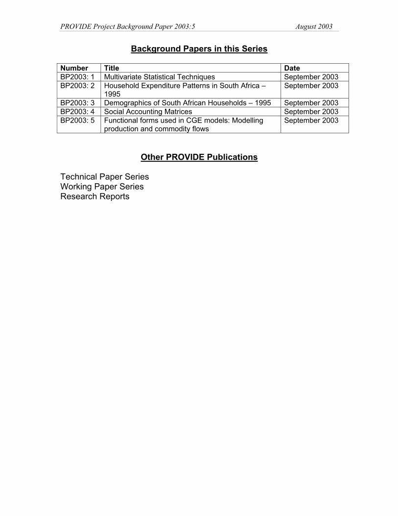
Background Papers in this Series Number Title Date BP2003: 1 Multivariate Statistical Techniques September 2003 BP2003: 2 Household Expenditure Patterns in South Africa –

1995 September 2003

BP2003: 3 Demographics of South African Households – 1995 September 2003 BP2003: 4 Social Accounting Matrices September 2003 BP2003: 5 Functional forms used in CGE models: Modelling

production and commodity flows September 2003

Other PROVIDE Publications Technical Paper Series Working Paper Series Research Reports

Background Paper 2003:5 - AgEcon Searchageconsearch.umn.edu/bitstream/15606/1/bp030005.pdf ·...

Documents

Transcript of Background Paper 2003:5 - AgEcon Searchageconsearch.umn.edu/bitstream/15606/1/bp030005.pdf ·...