BACKGROUND ON FINAL DISTRIBUTED PRIOR TO EXAM

The final will be set as a case study of Shaffer Substandard Auto Company. This means that you will be

using the same set up for all the problems. It also means that you are using the same data for several

problems. This should actually save you some time. However, since the format will be a little different, I

wanted to let you know ahead of time. Here is the case study scenario.

Shaffer sells automobile insurance to drivers who have a bad driving record. Each policy only covers one

automobile. During the exam, you will be studying the results of three years – 2011, 2012, and 2013.

During 2011, Shaffer had 10,000 policies. Each policy paid for 100% of all claims. In other words, there

were no deductibles, no upper limit, and no coinsurance. A policy can have more than one claim on an

automobile. You will then be given the results for 2011 and will be fitting models or the parameters for

models to this data. You could also be asked to do other calculations such as bootstrap the MSE.

During 2012, Shaffer modifies its auto insurance policy by implementing an upper limit per claim of

10,000. There remains no deductible and no coinsurance. Once again, you are given the data for 2012

and will be fitting models or the parameters for the models to this data.

Finally, in 2013, Shaffer has again revised the insurance policy sold by instituting a deductible per claim

of 500. The Company also instituted an upper limit per insurance policy of 25,000. You will be

expected to project the claims for 2013 using simulation.

There are 15 questions and 140 points on the final. While the stem to the problems all revolve around

the case study scenario, each problem stands on its own. In other words, your answer to one problem

does not get used in another problem. However, since you are dealing with the same data, there may

be some time savings. For example, if you are using the same sample data with in multiple problems,

you should only need to calculate the mean and variance of the sample once.

In order to complete all the tasks necessary, Kristin, who is the chief actuary for Shaffer, hires various

consultants to complete each of the 15 problems. For example, McReynolds Moment Matchers is hired

to complete one of the problems. (Guess what this problem is about.) All in all, as you take the test,

you will see Kristin hires ten consultants from this class to complete various tasks. In the end, we can

conclude that Shaffer’s biggest problem is TOO MANY CONSULTANTS!

STAT 479

Spring 2012

Final

Schaffer Substandard Auto Company sells automobile insurance to drivers who have a bad driving

record. Each policy only covers one automobile.

During 2011, Shaffer had 10,000 policies. Each policy paid for 100% of all claims. In other words, there

were no deductibles, no upper limit, and no coinsurance.

During 2011, the number of claims per insured automobile for Shaffer Substandard Auto Company was:

Number of Accidents in 2011 Number of Policies

0 2400

1 3400

2 2400

3 1500

4 300

1. (10 points) Kristin, the company’s actuary, hires Kelli from Chupp Consultants. Kelli models the

data as a Poisson distribution. Calculate the 90% linear confidence interval for based on the

above data.

Solution:

3400 (2)(2400) (3)(1500) (4)(300)ˆ 1.3910,000

ˆ 1.39ˆ[ ] 0.00013910,000

90% 1.39 1.645 0.000139 (1.3706,1.40904)

X

Varn

Confidence Interval =>

During 2011, the number of claims per insured automobile for Shaffer Substandard Auto Company was:

Number of Accidents in 2011 Number of Policies

0 2400

1 3400

2 2400

3 1500

4 300

The above data is repeated from the first page.

2. (10 points) Kelli also models the number of claims as a binomial distribution. She uses the

Method of Moments to estimate m and q . Determine Kelli’s estimate of m and q .

Solution:

2 2 2 22

2

[ ] 1.39

(1 )(3400) (2 )(2400) (3 )(1500) (4 )(300)[ ] 3.13

10,000

[ ] 3.13 1.39 1.1979

1.39 (1 ) 1.1979

(1 ) 1.1979 1.19791 1 0

1.39 1.39

E X See Question 1

E X

Var X

Under Binomial

mq and mq q

mq qq q

mq

.1382

1.39ˆ 10.058 10

0.1382

1.39ˆ 0.139

10

m m since m must be an integer

q=

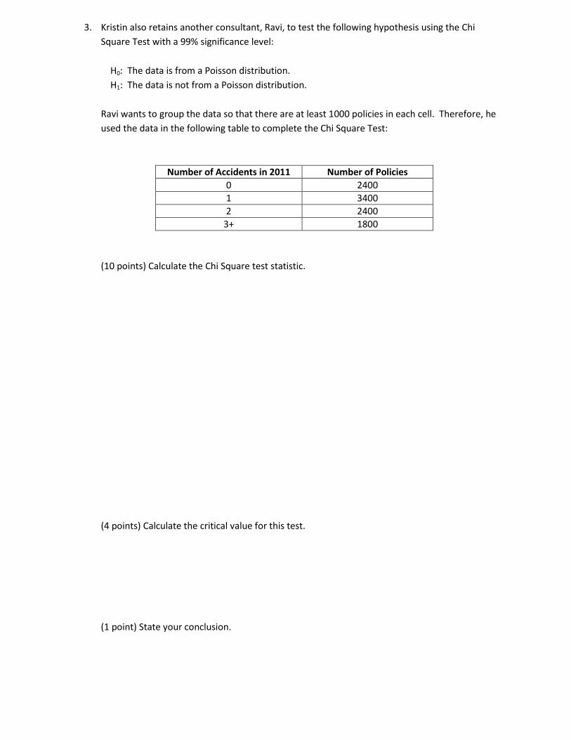
3. Kristin also retains another consultant, Ravi, to test the following hypothesis using the Chi

Square Test with a 99% significance level:

H0: The data is from a Poisson distribution.

H1: The data is not from a Poisson distribution.

Ravi wants to group the data so that there are at least 1000 policies in each cell. Therefore, he

used the data in the following table to complete the Chi Square Test:

Number of Accidents in 2011 Number of Policies

0 2400

1 3400

2 2400

3+ 1800

(10 points) Calculate the Chi Square test statistic.

(4 points) Calculate the critical value for this test.

(1 point) State your conclusion.

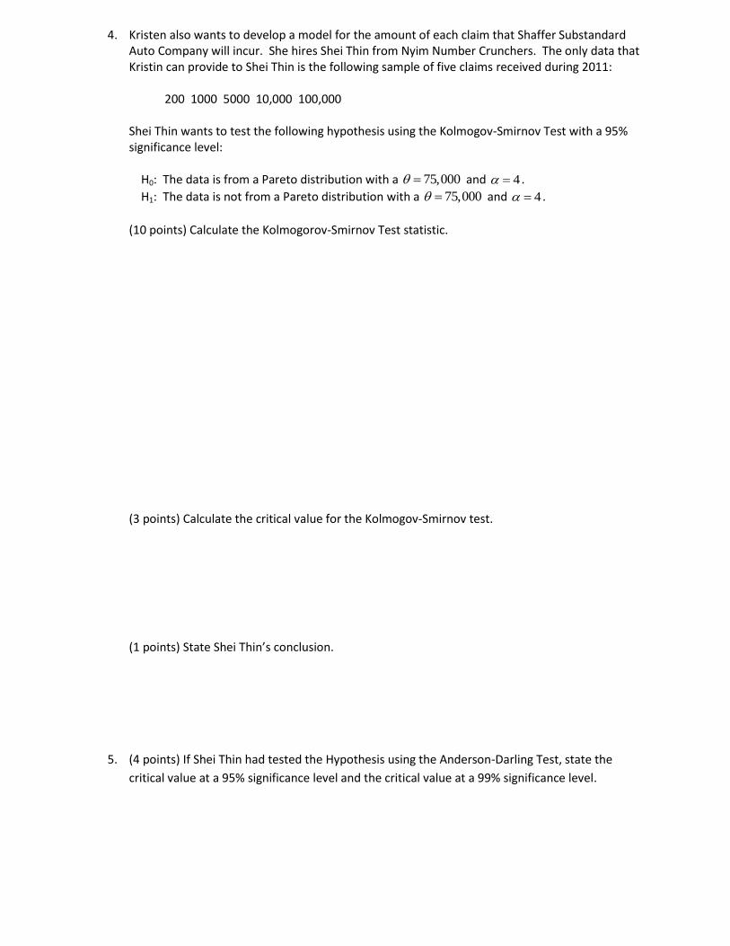
4. Kristen also wants to develop a model for the amount of each claim that Shaffer Substandard Auto Company will incur. She hires Shei Thin from Nyim Number Crunchers. The only data that Kristin can provide to Shei Thin is the following sample of five claims received during 2011: 200 1000 5000 10,000 100,000 Shei Thin wants to test the following hypothesis using the Kolmogov-Smirnov Test with a 95% significance level: H0: The data is from a Pareto distribution with a 75,000 and 4 .

H1: The data is not from a Pareto distribution with a 75,000 and 4 .

(10 points) Calculate the Kolmogorov-Smirnov Test statistic. (3 points) Calculate the critical value for the Kolmogov-Smirnov test. (1 points) State Shei Thin’s conclusion.

5. (4 points) If Shei Thin had tested the Hypothesis using the Anderson-Darling Test, state the

critical value at a 95% significance level and the critical value at a 99% significance level.

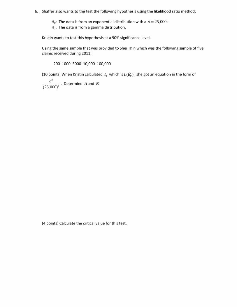
6. Shaffer also wants to the test the following hypothesis using the likelihood ratio method: H0: The data is from an exponential distribution with a 25,000 .

H1: The data is from a gamma distribution. Kristin wants to test this hypothesis at a 90% significance level. Using the same sample that was provided to Shei Thin which was the following sample of five claims received during 2011: 200 1000 5000 10,000 100,000 (10 points) When Kristin calculated

0L which is ( )L 0θ , she got an equation in the form of

(25,000)

A

B

e. Determine A and B .

(4 points) Calculate the critical value for this test.

7. (4 points) While Shei Thin is completing her work, Kristin decides to take the same sample and

model the amount of claims as uniformly distributed on the range of (0,U).

The sample was the following five claims received during 2011:

200 1000 5000 10,000 100,000

Calculate the maximum likelihood estimate of U.

Solution:

MLE of U is MAX(200 1000 5000 10,000 100,000) = 100,000

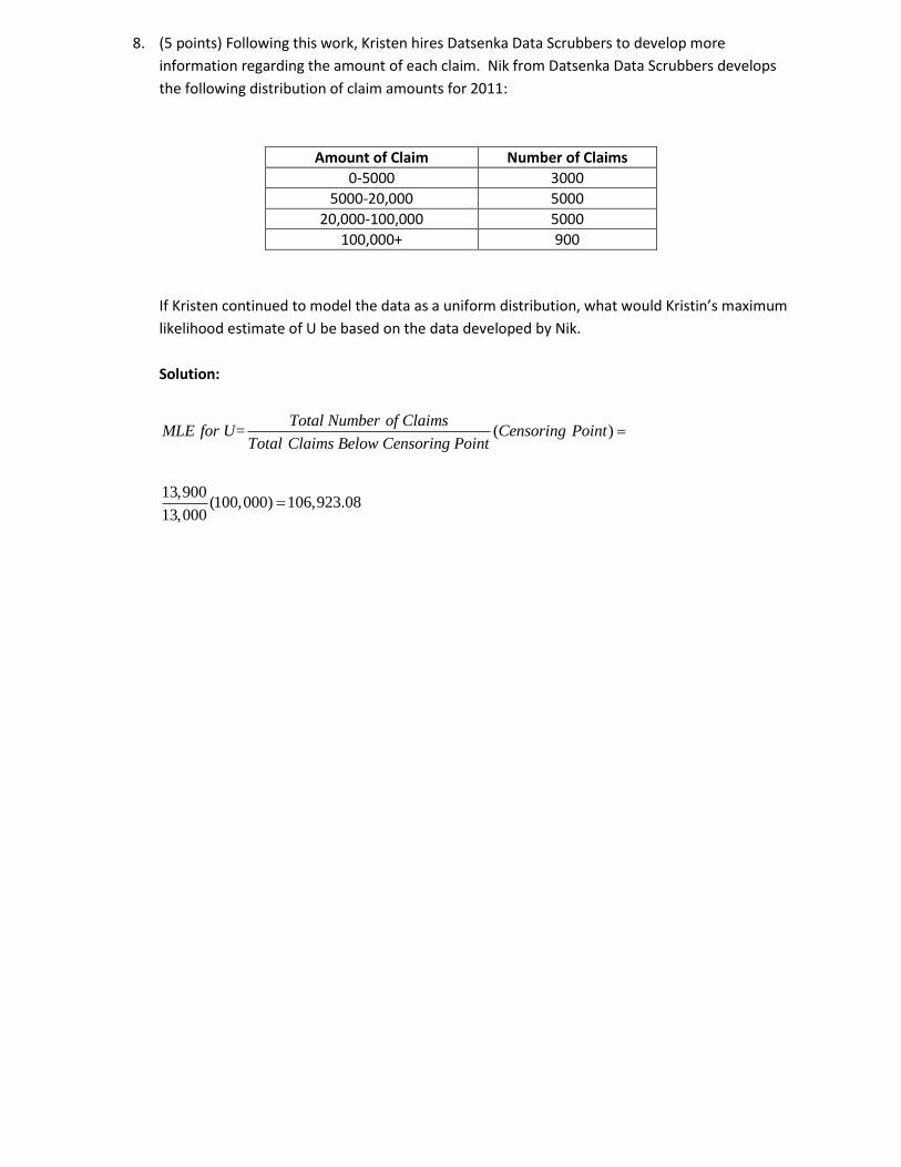
8. (5 points) Following this work, Kristen hires Datsenka Data Scrubbers to develop more

information regarding the amount of each claim. Nik from Datsenka Data Scrubbers develops

the following distribution of claim amounts for 2011:

Amount of Claim Number of Claims

0-5000 3000

5000-20,000 5000

20,000-100,000 5000

100,000+ 900

If Kristen continued to model the data as a uniform distribution, what would Kristin’s maximum

likelihood estimate of U be based on the data developed by Nik.

Solution:

( )

13,900(100,000) 106,923.08

13,000

Total Number of ClaimsMLE for U= Censoring Point

Total Claims Below Censoring Point

9. (10 points) Shaffer is also interested in calculating the median of the distribution of aggregate

claims per policy. The median of the distribution will be estimated as the average of the largest

and smallest values in a sample. In other words,

1 2 1 20.50

( , ,..., ) ( , ,..., )ˆ

2

n nMin X X X Max X X X

The following sample is selected from the distribution:

15,000 15,000 40,000

Using the bootstrap method, estimate the mean square error in the above estimator.

During 2012, Shaffer modifies its auto insurance policy by implementing an upper limit per claim of

10,000. There remains no deductible and no coinsurance.

The first four claims received during 2012 resulted in payments of:

800 4000 10,000 and 10,000

This sample will be used for questions 10-12.

10. (5 points) Shaffer hired Ellie’s Exponential Consulting Firm. Ellie assumes that the total claim

amount is distributed as an exponential distribution with a mean of .

Calculate the maximum likelihood estimate of .

Solution:

800 4000 10,000 10,000ˆ 12,4002

Total Amount Paid

Number of Uncensored Observations

During 2012, Shaffer modifies its auto insurance policy by implementing an upper limit per claim of

10,000. There remains no deductible and no coinsurance.

The first four claims received during 2012 resulted in payments of:

800 4000 10,000 and 10,000

This sample will be used for questions 10-12.

11. (10 points) Still not satisfied, Shaffer also retains The Wang Consulting Group to estimate the

parameters for an exponential distribution. One of Wang’s three partners, Shu, estimates

using the Method of Percentile Matching using the 25th percentile.

Determine Shu’s estimate of .

During 2012, Shaffer modifies its auto insurance policy by implementing an upper limit per claim of

10,000. There remains no deductible and no coinsurance.

The first four claims received during 2012 resulted in payments of:

800 4000 10,000 and 10,000

This sample will be used for questions 10-12.

12. (10 points) Shaffer also hires the consulting firm of Utomo & Guo to analyze the claims. Hassan,

the consultant from Utomo & Guo, assumes that the total claim amount is distributed as a

Weibull distribution with parameters 1 and .

Hassan uses the maximum likelihood estimate to estimate . What was Hassan’s estimate

of .

13. (10 points) Shaffer receives five more claims. The amount of each claim is

1000 4000 10,000 30,000 50,000

Using only this sample (and not data from the previous sample) , Shaffer wants to develop a

model for the total claim amount. Kristin, the company’s actuary, is now convinced that total

claims should be modeled as a Gamma distribution. She hires McReynolds Moment Matchers

to calculate the parameters of the Gamma distribution. McReynolds determines the

parameters using the Method of Moments.

Determine the estimates of and determined by McReynolds.

In 2013, Shaffer has again revised the insurance policy sold by instituting a deductible per claim of 500.

The Company also instituted an upper limit per insurance policy of 25,000.

14. (12 points) Shaffer Substandard Auto Company hires Shu Lei Simulators to simulate claim

payments for 2013.

Shu Lei assumes that the number of claims is distributed as a binomial distribution with 5m

and 0.4q .

Shu Lei also assumes that the amount of each claim is distributed as an exponential distribution

with θ = 20,000.

Using simulation, Shu Lei wants to estimate the total claims that will need to be paid under the

revised policy. She does so by estimating the claims for each insured. Sze-Ie and Booi Yee are

the first two insureds. First, Shu Lei determines the number of claims for Sze-Ie and then the

amount of each claim for Sze-Ie. Next, Shu Lei determines the number of claims for Booi Yee.

Finally, Shu Lei simulates the amount of each of Booi Yee‘s claims.

The random numbers used in the simulation are:

0.40 0.02 0.20 0.80 0.25 0.50 0.30 0.60 0.95 0.75 0.05

Calculate the simulated aggregate claim payments for Sze-Ie and the simulated aggregate claim

payments for Booi Yee.

15. During this wonderful exam, Shaffer has modeled claim amounts using the following

distributions: Exponential, Gamma, Pareto, Weibull, and Uniform. The concept of parsimony

provides guidance in choosing a model.

a. (3 points) State the concept of parsimony.

b. (3 points) If you were hired as a consultant to Shaffer, state which model you would

chose based simply on the concept of parsimony and explain why this model would be

consistent with parsimony.

16. BONUS: What is Shaffer Substandard Auto Company’s biggest problem?