Background intensity correction for terabyte‐sized time ... · tal artefacts without recorded...

Journal of Microscopy, Vol. 257, Issue 3 2015, pp. 226–237 doi: 10.1111/jmi.12205

Received 25 March 2014; accepted 14 November 2014

Background intensity correction for terabyte-sized time-lapseimages

J . C H A L F O U N ∗, M . M A J U R S K I ∗, K . B H A D R I R A J U†, S . L U N D ∗, P . B A J C S Y ∗ & M . B R A D Y ∗∗Information Technology Laboratory, National Institute of Standards and Technology, Gaithersburg, Maryland, U.S.A.

†Material Measurement Laboratory, National Institute of Standards and Technology, Gaithersburg, Maryland, U.S.A.

Key words. Background modelling, fluorescent image correction, imagemosaic, large field of view.

Summary

Several computational challenges associated with large-scalebackground image correction of terabyte-sized fluorescent im-ages are discussed and analysed in this paper. Dark current,flat-field and background correction models are applied overa mosaic of hundreds of spatially overlapping fields of view(FOVs) taken over the course of several days, during whichthe background diminishes as cell colonies grow. The motiva-tion of our work comes from the need to quantify the dynamicsof OCT-4 gene expression via a fluorescent reporter in humanstem cell colonies. Our approach to background correction isformulated as an optimization problem over two image par-titioning schemes and four analytical correction models. Theoptimization objective function is evaluated in terms of (1) theminimum root mean square (RMS) error remaining after im-age correction, (2) the maximum signal-to-noise ratio (SNR)reached after downsampling and (3) the minimum executiontime. Based on the analyses with measured dark current noiseand flat-field images, the most optimal GFP background cor-rection is obtained by using a data partition based on forming aset of submosaic images with a polynomial surface backgroundmodel. The resulting image after correction is characterized byan RMS of about 8, and an SNR value of a 4 × 4 downsam-pling above 5 by Rose criterion. The new technique generatesan image with half RMS value and double SNR value whencompared to an approach that assumes constant backgroundthroughout the mosaic. We show that the background noisein terabyte-sized fluorescent image mosaics can be correctedcomputationally with the optimized triplet (data partition,model, SNR driven downsampling) such that the total RMSvalue from background noise does not exceed the magnitude ofthe measured dark current noise. In this case, the dark currentnoise serves as a benchmark for the lowest noise level that animaging system can achieve. In comparison to previous work,

Correspondence to: Peter Bajcsy, Information Technology Laboratory, National In-

stitute of Standards and Technology, 100 Bureau Drive, Gaithersburg, MD 20899,

U.S.A. Tel: 3019752958; fax: 301-975-6097; e-mail: [email protected]

the past fluorescent image background correction methodshave been designed for single FOV and have not been appliedto terabyte-sized images with large mosaic FOVs, low SNR anddiminishing access to background information over time ascell colonies span entirely multiple FOVs. The code is availableas open-source from the following link https://isg.nist.gov/.

Background

Pluripotent stem cells have great potential as a source of cellsfor regenerative therapies. However, many aspects of control-ling pluripotent stem cells behaviour are still not well under-stood (Saha & Jaenisch, 2009). The motivation of our workcomes from the need to quantify the dynamics of OCT-4 geneexpression in human stem cell colonies, because OCT-4 is acritical gene in the regulation of pluripotency, or the abil-ity of stem cells to differentiate into all somatic cell types(VanDenBerg et al., 2010). OCT-4 gene expression in cells isreported by a green fluorescent protein (GFP) reporter insertedin the regulatory region of the OCT-4 gene (Zwaka & Thomson,2003). Specifically, we are interested in understanding howcolony-level GFP intensity is related to population-level cellbehaviour, how normal regulation of stem cell gene expres-sion occurs, and how to develop and assess human pluripotentstem cells culture quality parameters.

Time-lapse epifluorescence microscopy using fluorescentprotein reporters provides an opportunity for imaging andanalysing the dynamics of gene expression and morpholog-ical changes in live human pluripotent stem cells cultures.Imaging at high spatial and temporal resolutions generatesterabyte-sized image sets spanning hundreds of FOVs throughtime (Fig. 1). There are several technical challenges to over-come before quantitative biological information can be ob-tained from these big data sets. Images of live cells, such aspluripotent stem cells, must be acquired with low-power illu-mination to minimize biological artefacts from light-induceddamage to cells. Light intensity was empirically set at the low-est value, at which we could still discern image features in each

Published 2014. This article is a U.S. Government work and is in the public domain in the USA

B A C K G R O U N D I N T E N S I T Y C O R R E C T I O N 2 2 7

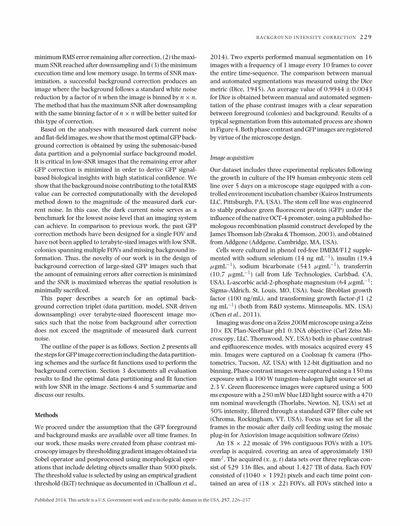
Fig. 1. Uncorrected and flat-field corrected example image: Uncorrected mosaic of green fluorescent protein (GFP) image channel that was stitched from22 × 18 FOVs acquired on the fourth day of a stem cell colony imaging experiment (left). The image on the right is corrected for uneven illumination anddark current but not corrected for background. The five numbered red ‘x’ mark FOVs with nothing but background pixels in them.

Fig. 2. Normalized histogram of foreground and background intensities: Foreground and background normalized histograms of one image with 500bins. The two curves illustrate low SNR = 1.4 in the (1 × 1) binned GFP image.

respective colour channel and could perform image analy-sis. The acquisition requirement of minimally perturbing cellsleads to a low signal-to-noise ratio (SNR) of the fluorescentsignal (Fig. 2) and its sensitivity to correcting for dark current,flat-field and background media sources of noise. We addressthe overall problem of fluorescent image correction with thefocus on background correction in order to minimize the re-maining errors in the corrected background and maximize theSNR.

The background correction poses challenges due to the com-plex interactions of cells, media, fluorescent biomarker andimaging light, and also due to the computational demands ofprocessing images spanning very large fields of view of grow-ing cell colonies. In general, the foreground intensity signalover cell colony image regions includes not only contributionsfrom cells but also non-specific autofluorescence from the cellculture media, culture dish and any extracellular matrix pro-tein coatings (Fig. 3). The fluorescent components may vary

Published 2014. This article is a U.S. Government work and is in the public domain in the USA, 257, 226–237

2 2 8 J . C H A L F O U N E T A L .

Fig. 3. Spatiotemporal graphs of average intensity per FOV: These results are displayed for the five numbered locations shown in Figure 1 through 5 daysof acquisition. A frame is acquired every 45 min and a daily media change for the culture is performed every 24 h from the beginning of the experiment.The curves illustrate global intensity variations across an entire image mosaic and over time.

spatially and temporally because of spatial distribution of fluo-rescent molecules, different amounts of light interacting withthese molecules, and photo-bleaching of molecules over time.It is impossible to capture these spatiotemporal variations offluorescent signal in the background from a single FOV sincestem cell colonies grow to cover very large spatial areas. Fur-thermore, the background correction is complicated by the factthat individual colonies can completely occupy areas spanningseveral FOVs, creating FOVs without any background pixels(Fig. 1). Unlike single cell imaging where background areasaround cells provide accurate estimates of background inten-sity, pluripotent stem cells grow as colonies of cells (islands)that merge with neighbouring colonies over time as the cultureprogresses, and background areas in a colony culture becomesparse at later times. In summary, background correction fromlive stem cell colony microscopy experiments has to overcomeestimation challenges including: (1) finding accurate spatialand temporal models, (2) deriving parameters of the modelsfrom a diminishing number of background pixels over time ascolonies grow, (3) maximizing SNR due to low-light illumina-tion and (4) scaling computations of background models overa very large mosaic of small FOVs, and hence millions of pixelvalues per time frame.

The problem of correcting single FOV images has been ap-proached by imaging reference materials (Model & Burkhardt,2001), designing data-driven models of optical and digi-tal artefacts without recorded images of reference materi-als (Leong, 2003), or combining both recorded images ofreference materials and data-driven models (Piccinini et al.,2013). The past work spans commercial panoramic cameras(Goldman, 2010), microscope cameras (Waters & Swedlow,2007; Wu et al., 2008), and various custom cameras (Kim

& Pollefeys, 2008; Galego, 2011). Many techniques for esti-mating vignetting (radial fall-off), exposure and white balancevariations, and sample radiances are common across multi-ple camera types including the microscope cameras with spe-cific challenges summarized by Waters & Swedlow (2007).Some background correction models are approximated bythe mean grey level of the areas between cells (Model &Burkhardt, 2001). A more accurate background subtractioncan be achieved by extracting average grey level from prede-fined surrounding pixels of a cell or a colony (Chalfoun et al.,2013). This cell/colony specific background value compen-sates for spatial variations better than a single mean grey levelespecially for data sets with large FOVs and acquired over asignificant duration of time.

None of the previous work deals with background mea-surement or modelling over large image mosaics and in thepresence of cells/colonies that cover multiple FOVs. The back-ground is usually considered constant or is neglected. In moreadvanced treatment, background is approximated by averag-ing closest background pixels to the cell areas or estimated by afitting function on the entire FOV pixels. These approaches donot work well on large spatial mosaics due to computationalcomplexity (execution time and machine memory usage) andthe need to model the background across large numbers ofFOVs.

Our approach to background correction is formulated as anoptimization problem over two data partitioning schemes (fullmosaic and submosaic based) and their corresponding cor-rection models represented by four analytical functions. Thefour functions include polynomial surface, cubic spline in-terpolation, linear interpolation and nearest neighbour. Theoptimization objective function is evaluated in terms of (1) the



minimum RMS error remaining after correction, (2) the maxi-mum SNR reached after downsampling and (3) the minimumexecution time and low memory usage. In terms of SNR max-imization, a successful background correction produces animage where the background follows a standard white noisereduction by a factor of n when the image is binned by n × n.The method that has the maximum SNR after downsamplingwith the same binning factor of n × n will be better suited forthis type of correction.

Based on the analyses with measured dark current noiseand flat-field images, we show that the most optimal GFP back-ground correction is obtained by using the submosaic-baseddata partition and a polynomial surface background model.It is critical in low-SNR images that the remaining error afterGFP correction is minimized in order to derive GFP signal-based biological insights with high statistical confidence. Weshow that the background noise contributing to the total RMSvalue can be corrected computationally with the developedmethod down to the magnitude of the measured dark cur-rent noise. In this case, the dark current noise serves as abenchmark for the lowest noise level that an imaging systemcan achieve. In comparison to previous work, the past GFPcorrection methods have been designed for a single FOV andhave not been applied to terabyte-sized images with low SNR,colonies spanning multiple FOVs and missing background in-formation. Thus, the novelty of our work is in the design ofbackground correction of large-sized GFP images such thatthe amount of remaining errors after correction is minimizedand the SNR is maximized whereas the spatial resolution isminimally sacrificed.

This paper describes a search for an optimal back-ground correction triplet (data partition, model, SNR drivendownsampling) over terabyte-sized fluorescent image mo-saics such that the noise from background after correctiondoes not exceed the magnitude of measured dark currentnoise.

The outline of the paper is as follows. Section 2 presents allthe steps for GFP image correction including the data partition-ing schemes and the surface fit functions used to perform thebackground correction. Section 3 documents all evaluationresults to find the optimal data partitioning and fit functionwith low SNR in the image. Sections 4 and 5 summarize anddiscuss our results.

Methods

We proceed under the assumption that the GFP foregroundand background masks are available over all time frames. Inour work, these masks were created from phase contrast mi-croscopy images by thresholding gradient images obtained viaSobel operator and postprocessed using morphological oper-ations that include deleting objects smaller than 5000 pixels.The threshold value is selected by using an empirical gradientthreshold (EGT) technique as documented in (Chalfoun et al.,

2014). Two experts performed manual segmentation on 16images with a frequency of 1 image every 10 frames to coverthe entire time-sequence. The comparison between manualand automated segmentations was measured using the Dicemetric (Dice, 1945). An average value of 0.9944 ± 0.0043for Dice is obtained between manual and automated segmen-tation of the phase contrast images with a clear separationbetween foreground (colonies) and background. Results of atypical segmentation from this automated process are shownin Figure 4. Both phase contrast and GFP images are registeredby virtue of the microscope design.

Image acquisition

Our dataset includes three experimental replicates followingthe growth in culture of the H9 human embryonic stem cellline over 5 days on a microscope stage equipped with a con-trolled environment incubation chamber (Kairos InstrumentsLLC, Pittsburgh, PA, USA). The stem cell line was engineeredto stably produce green fluorescent protein (GFP) under theinfluence of the native OCT-4 promoter, using a published ho-mologous recombination plasmid construct developed by theJames Thomson lab (Zwaka & Thomson, 2003), and obtainedfrom Addgene (Addgene, Cambridge, MA, USA).

Cells were cultured in phenol red-free DMEM/F12 supple-mented with sodium selenium (14 ng mL−1), insulin (19.4μgmL−1), sodium bicarbonate (543 μgmL−1), transferrin(10.7 μgmL−1) (all from Life Technologies, Carlsbad, CA,USA), L-ascorbic acid-2-phosphate magnesium (64 μgmL−1;Sigma-Aldrich, St. Louis, MO, USA), basic fibroblast growthfactor (100 ng/mL), and transforming growth factor-β1 (2ng mL−1) (both from R&D systems, Minneapolis, MN, USA)(Chen et al., 2011).

Imaging was done on a Zeiss 200M microscope using a Zeiss10× EX Plan-NeoFluar ph1 0.3NA objective (Carl Zeiss Mi-croscopy, LLC, Thornwood, NY, USA) both in phase contrastand epifluorescence modes, with mosaics acquired every 45min. Images were captured on a Coolsnap fx camera (Pho-tometrics, Tucson, AZ, USA) with 12-bit digitization and nobinning. Phase contrast images were captured using a 150 msexposure with a 100 W tungsten–halogen light source set at2.3 V. Green fluorescence images were captured using a 500ms exposure with a 250 mW blue LED light source with a 470nm nominal wavelength (Thorlabs, Newton, NJ, USA) set at50% intensity, filtered through a standard GFP filter cube set(Chroma, Rockingham, VT, USA). Focus was set for all theframes in the mosaic after daily cell feeding using the mosaicplug-in for Axiovision image acquisition software (Zeiss)

An 18 × 22 mosaic of 396 contiguous FOVs with a 10%overlap is acquired, covering an area of approximately 180mm2. The acquired (x, y, t) data sets over three replicas con-sist of 529 336 files, and about 1.427 TB of data. Each FOVconsisted of (1040 × 1392) pixels and each time point con-tained an area of (18 × 22) FOVs, all FOVs stitched into a


2 3 0 J . C H A L F O U N E T A L .

Fig. 4. Segmentation example: Phase contrast image example (left). Corresponding segmented image overlaid on top of the phase image (right).

single time point mosaic consisting of approximately (20 000× 20 000) pixels. Flat-field images for the GFP channel werecollected using a fluorescent solution sandwiched between aglass slide and a coverslip, as previously described (Model &Burkhardt, 2001).

Flat-field and dark current correction

In our work, we are interested primarily in fluorescent micro-scope image correction models that compensate for thermalnoise (dark current models), uneven illumination (vignettingfunctions) and stem cell media interaction (background cor-rection methods). The dark current and vignetting functionsare modelled using recorded single FOV images. We follow astandard calibration procedure described in Eq. (1) that utilizesrecorded dark current images acquired with a closed camerashutter and fluorescein images obtained by imaging a refer-ence fluorescent solution (Model & Burkhardt, 2001). In thisstudy, we are not concerned with photo-bleaching, autofluo-rescence, CCD readout and quantization noise since they rep-resent standalone problems (Wu et al., 2008). The calibrationis represented by Eq. (1).

GFPsignal = I − B − DF − D

= I − DF − D

− B f , (1)

where I is the intensity of an acquired image, D is the darkimage, F is the fluorescein image and B is the backgroundimage, the offset information present in I. Note that, B f is thebackground image after flat-field correction. Through the restof the paper all estimation models and analysis are done tomeasure B f .

Optimization framework for background correction

Evaluation of background correction error. For the purpose ofevaluating estimated background, we established a set of back-ground reference pixels (BRP) through the following process,which is displayed in Figure 5: The BRP of any given image arethe set of pixel locations that belong to the background (BK G )of that image and the foreground (F RG ) of the latest image inthe given time-sequence dataset (B RP = F RG latest ∩B K G ).These are the pixels of known background values but consid-ered as unknown when performing the background correc-tion. When fitting the model we use pixels that are containedin the background BK G but not in the BRP. That is, the setBK G ∩B RP c is used for training and the set BRP is used fortesting.

Figure 5 shows segmentation of an early time point (t = 50× 45 min = 37.5 h from the first acquisition on the left). Themiddle mask shows the background pixels that were consid-ered for model fitting. The third mask shows the backgroundpixels from the latest time point (t = 161 × 45 min = 120.75h from the first acquisition) that were omitted from the fitand used to compute the remaining error in the backgroundcorrection.

When applying background correction techniques to theflat-field and dark current corrected GFP images, different re-sults of corrected images are obtained. In order to evaluatemultiple background correction techniques, we define an op-timization objective function in Eq. (2) with the search spacesamples. We search for an optimal data partitioning schemeand background correction model that achieve (1) the mini-mum RMS of the difference between the modelled backgroundintensities and the observed intensities over the BRP (Fig. 5),(2) maximum SNR and (3) minimum execution time (Texec).



Fig. 5. Three regions of interest: Three regions of interest: Segmented image with all available background pixels labelled as white (left). Segmented imagewith background pixels used for the fit modelling in white (middle). Segmented image where background reference pixels (BRP) in white were used forevaluating the remaining error as RMS value.

After successful background correction the image SNR is in-creased by downsampling (replacing a group of neighbouringpixels by their average value). The method that has the maxi-mum SNR after downsampling with the same binning factor ofn×n will be better suited for this type of correction. Each term ofthe optimization objective function in Eq. (2) is given a weightdetermined by its importance. In our experiments, the weightsfollowed the ratio wRMS : wSN R : wT e xec = 3 : 2 : 1. The val-ues of RMS, SNR and Texec were normalized with respect tomaximum RMS value, maximum SNR value, and maximumexecution time per time point. All of the terms in the followingequations will be described in the following subsections.

Optimization function:

{DataPartition, Model}∗ =arg min{DataPartition,Model} (wRMS ∗ RMS

+wSNR ∗ (1−SNR)+wTexec ∗ Texec) . (2)

Search space:

DataPartition = {full mosaic, submosaic} .

Model = {polynomial surface, cubic interpolation, linear

interpolation, nearest neighbor} .

SNR and the RMS error of a given image are computedaccording to the equations below:

SN R = 1NF RG

∑n∈F RG

(In − B̂n)/std({

In − B̂n}

n∈BK G

), (3)

RMS =√

1NB RP

∑n∈B RP

(In − B̂n

)2, (4)

where in Eqs. (3) and (4), NF RG and NB RP denote the numberof foreground pixels and BRP, respectively, n is an index forpixel location in the image, In is the observed intensity of pixeln, B̂n is the modelled background intensity of pixel n, F RG isthe set of pixel locations that are identified as foreground andBK G is the complement of F RG and contains the set of pixelsidentified as background, B RP is a subset of BK G used forbackground model assessment.

Data partitioning schemes and surface fit functions. We haveconsidered two image partitioning schemes, the full mosaicand submosaic-based partitions. Figures 6 and 7 illustrateboth data partitioning schemes. Submosaic images in Figure 7are created by extracting the average value of a sub tile (anexample of a subtile is the red square in the upper left cornerof a FOV) from each FOV at a fixed location and placing it intoa constructed submosaic image according to the FOV index inthe grid of FOVs per time frame. Each FOV has a dimension of(1040 × 1392). For a subtile size of 16 × 16 pixels, each FOVwill be tiled into 65 × 87 = 5655 subtiles. Each subtile at aparticular location will be replaced by the average value over16 × 16 pixels. These values from the same location acrossall FOVs (the red for example) will be assembled together toform one submosaic. Each submosaic will have a size of (18× 22) pixels. The total number of submosaics formed is 5655.The surface fit will be applied on each mosaic independently.Figure 8 shows the submosaic images formed from the (18 ×22) grid of FOVs. The black pixels indicate that they belongto the foreground and hence are not available for backgroundmodelling. The idea behind the submosaic creation is thatbackground intensities are continuous throughout the entireplate and across FOV boundaries. The submosaic image is agood approximated map of the background throughout theentire mosaic representing a particular FOV location.

For the optimization study, we used four surface fit-ting functions for correcting terabyte-sized GFP images


2 3 2 J . C H A L F O U N E T A L .

Fig. 6. Image partitioning scheme 1: Background intensity estimation by surface model fitting to an image mosaic based on available background pixels(nonblack pixels in the image on the left).

Fig. 7. Image partitioning scheme 2: Average values of the red pixels from the same location of all FOV are assembled into the red submosaic. The sameprocedure is performed on the pixels at the following location (the green one) etc. until all locations on the FOV have been assembled into submosaics.Background estimation by surface fitting is performed to the constructed submosaics. There are m = 18 times n = 22 equal to 396 FOVs used forbackground estimation. The red and green colours denote the original location of the pixels in each FOV and their new locations in a submosaic images.

Table 1. Surface fit functions.

Fit Type Description

Polynomial surface Z = p00 + p10*x + p01*y + . . . + p12*x*y2 + p03*y3

Cubic interpolating spline This method fits a different cubic polynomial between sets of three points for surfaces.Linear interpolation This method fits a different linear polynomial between sets of three points for surfaces.Nearest neighbour This method sets the value of an interpolated point to the value of the nearest data point.

as described in Table 1. The methods come directly fromthe Matlab library (with online documentation found in:http://www.mathworks.com/help/curvefit/fit.html) and aredescribed in detail in Rovenskii (2010).

ResultsFirst, we discuss the results of the best technique for GFP back-ground correction found from our optimization scheme. Then,we compute the best image mosaic downsampling to get theSNR to a minimum value of 5 per Rose criterion (Watts et al.,

2000) across all time points and replicas, which gives a goodSNR whereas minimal spatial resolution is sacrificed

Optimization results

We report optimization results performed on 15 time points inFigure 9 below. The time-points are selected by increment of10 frames. The execution time of the model fit is measured inseconds and it is the time needed to perform the background



Fig. 8. Resulting submosaic images over time: The decreasing number of background pixels is due to the growth of stem cell colonies. The submosaicimages on the left are at the early time points and on the right at the later time points of the experiment. Nonblack pixels in 18 × 22 submosaic images areat those FOV locations that contain only background pixels within a FOV. The black pixels in 18 × 22 submosaic images represent the average intensityvalue of the foreground pixels in that particular FOV.

Fig. 9. Results between image partitioning schemes: This figure displays the results for image partitioning approaches for 15 time-slices (one slice istaken every 10 frames). The four illustrations above represent the quality metrics for the eight partitioning-model combinations (two image partitioningschemes and four background interpolation models performed on 4 × 4 downsampled GFP images to meet the SNR constraint). The ‘score’ quality metricis computed according to Eq. (2) with the RMS, BRP, SNR and Texec normalized by the maximum values over both approaches.

estimation on a mosaic image at one time point. The overallexecution time including reading image tiles, model fit, back-ground correction and mosaic assembly takes about 15 minper time point. The optimization code was written in Matlab R©

[version 8.0.0.783 (R2012b)] with the additional packages‘image processing toolbox 8.1’ and ‘statistics toolbox 8.1’. The

code was executed on a desktop machine with Intel R© Xeon R©

CPU E5–2620 0 @ 2.00GHz, 64.0 GB RAM, and Windows 7Enterprise (64 bit) operating system.

The results displayed in Figure 9 indicate that for each ofthe four considered surface fit functions (see Table 1), theapproach based on fitting submosaic images achieves smaller


2 3 4 J . C H A L F O U N E T A L .

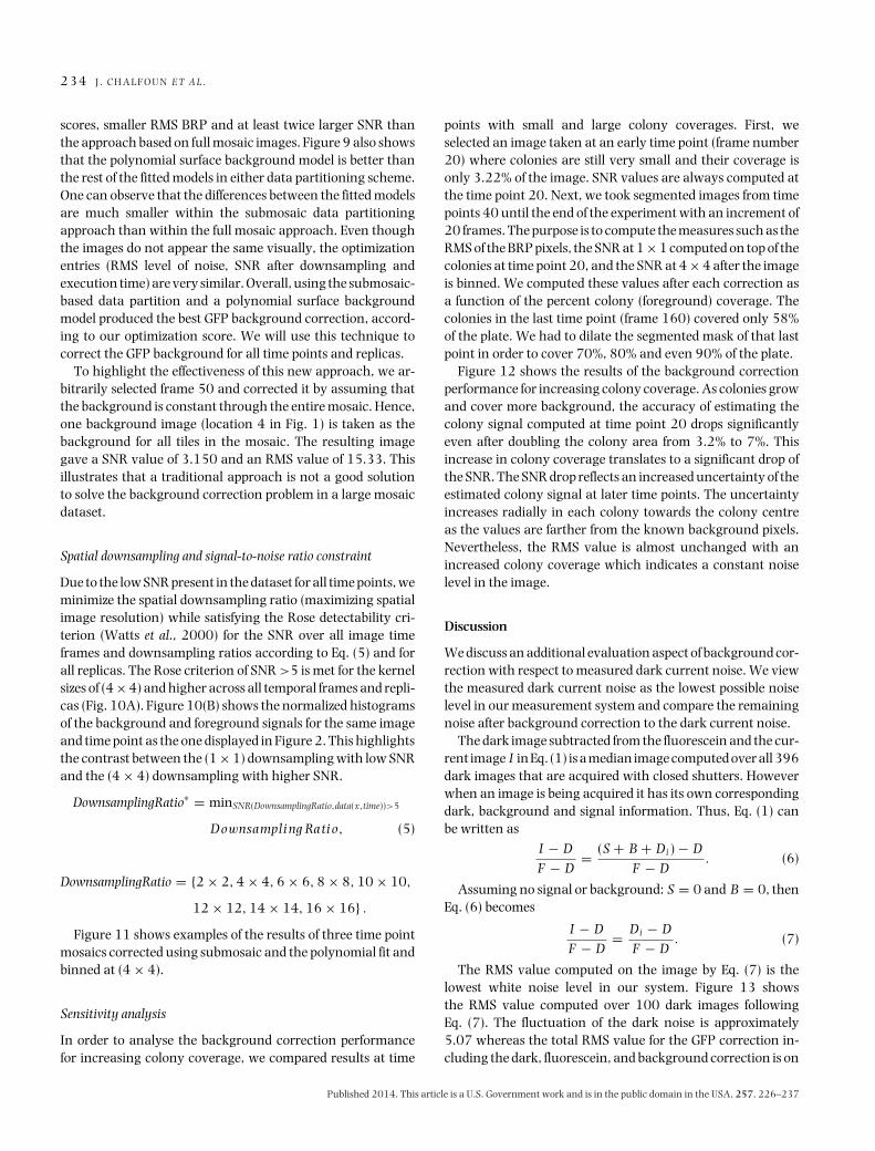
scores, smaller RMS BRP and at least twice larger SNR thanthe approach based on full mosaic images. Figure 9 also showsthat the polynomial surface background model is better thanthe rest of the fitted models in either data partitioning scheme.One can observe that the differences between the fitted modelsare much smaller within the submosaic data partitioningapproach than within the full mosaic approach. Even thoughthe images do not appear the same visually, the optimizationentries (RMS level of noise, SNR after downsampling andexecution time) are very similar. Overall, using the submosaic-based data partition and a polynomial surface backgroundmodel produced the best GFP background correction, accord-ing to our optimization score. We will use this technique tocorrect the GFP background for all time points and replicas.

To highlight the effectiveness of this new approach, we ar-bitrarily selected frame 50 and corrected it by assuming thatthe background is constant through the entire mosaic. Hence,one background image (location 4 in Fig. 1) is taken as thebackground for all tiles in the mosaic. The resulting imagegave a SNR value of 3.150 and an RMS value of 15.33. Thisillustrates that a traditional approach is not a good solutionto solve the background correction problem in a large mosaicdataset.

Spatial downsampling and signal-to-noise ratio constraint

Due to the low SNR present in the dataset for all time points, weminimize the spatial downsampling ratio (maximizing spatialimage resolution) while satisfying the Rose detectability cri-terion (Watts et al., 2000) for the SNR over all image timeframes and downsampling ratios according to Eq. (5) and forall replicas. The Rose criterion of SNR >5 is met for the kernelsizes of (4 × 4) and higher across all temporal frames and repli-cas (Fig. 10A). Figure 10(B) shows the normalized histogramsof the background and foreground signals for the same imageand time point as the one displayed in Figure 2. This highlightsthe contrast between the (1 × 1) downsampling with low SNRand the (4 × 4) downsampling with higher SNR.

DownsamplingRatio∗ = minSNR(DownsamplingRatio,data(x,time))>5

D ownsampli ng Rati o, (5)

DownsamplingRatio = {2 × 2, 4 × 4, 6 × 6, 8 × 8, 10 × 10,

12 × 12, 14 × 14, 16 × 16} .

Figure 11 shows examples of the results of three time pointmosaics corrected using submosaic and the polynomial fit andbinned at (4 × 4).

Sensitivity analysis

In order to analyse the background correction performancefor increasing colony coverage, we compared results at time

points with small and large colony coverages. First, weselected an image taken at an early time point (frame number20) where colonies are still very small and their coverage isonly 3.22% of the image. SNR values are always computed atthe time point 20. Next, we took segmented images from timepoints 40 until the end of the experiment with an increment of20 frames. The purpose is to compute the measures such as theRMS of the BRP pixels, the SNR at 1 × 1 computed on top of thecolonies at time point 20, and the SNR at 4 × 4 after the imageis binned. We computed these values after each correction asa function of the percent colony (foreground) coverage. Thecolonies in the last time point (frame 160) covered only 58%of the plate. We had to dilate the segmented mask of that lastpoint in order to cover 70%, 80% and even 90% of the plate.

Figure 12 shows the results of the background correctionperformance for increasing colony coverage. As colonies growand cover more background, the accuracy of estimating thecolony signal computed at time point 20 drops significantlyeven after doubling the colony area from 3.2% to 7%. Thisincrease in colony coverage translates to a significant drop ofthe SNR. The SNR drop reflects an increased uncertainty of theestimated colony signal at later time points. The uncertaintyincreases radially in each colony towards the colony centreas the values are farther from the known background pixels.Nevertheless, the RMS value is almost unchanged with anincreased colony coverage which indicates a constant noiselevel in the image.

Discussion

We discuss an additional evaluation aspect of background cor-rection with respect to measured dark current noise. We viewthe measured dark current noise as the lowest possible noiselevel in our measurement system and compare the remainingnoise after background correction to the dark current noise.

The dark image subtracted from the fluorescein and the cur-rent image I in Eq. (1) is a median image computed over all 396dark images that are acquired with closed shutters. Howeverwhen an image is being acquired it has its own correspondingdark, background and signal information. Thus, Eq. (1) canbe written as

I − DF − D

= (S + B + Di ) − DF − D

. (6)

Assuming no signal or background: S = 0 and B = 0, thenEq. (6) becomes

I − DF − D

= Di − DF − D

. (7)

The RMS value computed on the image by Eq. (7) is thelowest white noise level in our system. Figure 13 showsthe RMS value computed over 100 dark images followingEq. (7). The fluctuation of the dark noise is approximately5.07 whereas the total RMS value for the GFP correction in-cluding the dark, fluorescein, and background correction is on



Fig. 10. Downsampling and SNR plot: (A) SNR computed over all 161 temporal frames of replica 1 and spatial downsampling kernels between 2 × 2and 16 × 16. The Rose criterion of SNR > 5 is met for the kernel sizes of 4×4 and higher across all frames. (B) Foreground and background normalizedhistograms of one binned image (4 × 4) with 500 bins. The two curves illustrate a SNR = 6.1 in contrast with the SNR = 1.4 in the (1 × 1) binned image.

Fig. 11. Examples of corrected GFP images: Corrected images for frames 50, 100 and 150 from left to right. These images are spatially downsampled by(4 × 4), flat-field correction, dark current correction and background subtraction.

Fig. 12. Sensitivity analysis to the foreground percentile coverage: Image frame 20 is considered for this sensitivity analysis where colonies are still verysmall and cover only 3.22% of the image. SNR values are computed at the image frame 20. RMS values are computed over known background pixelsthat are considered unknown by taking segmented images from image frame 40 until the end of the experiment with an increment of 20 frames. Thecolonies at the end of the experiment cover 58%, morphological dilation is done to get the colony coverage to 90%.


2 3 6 J . C H A L F O U N E T A L .

Fig. 13. Dark images error: RMS error obtained over 100 single FOV images with only background pixels.

the order of 8.9. That gives a maximum error contribution ofe = 9.53 − 5.07 = 3.83 as total error from fluorescein andbackground correction. This error is less than the dark noiseerror contribution which demonstrates experimentally thatthe background noise contributing to the total RMS value canbe corrected computationally with the developed method to amagnitude less than the measured dark current noise.

Conclusions

We demonstrated a computational technique for backgroundcorrection of terabyte-sized fluorescent microscopy images.The solution was obtained by optimizing over a space of twoimage partitioning schemes and four background correctionmodels. The optimization cost function included RMS, SNRand execution time. We concluded that the optimal solutionframework contribution from background noise to the totalRMS value does not exceed the measured dark current noise.The new technique generated a corrected image with half ofthe error value and twice of the SNR value when compared toan approach that assumes constant background throughoutthe mosaic. We made the code is available as open-source fromthe following link https://isg.nist.gov/.

In the future, we plan to develop a temporal model of colonybackground which would include photo-bleaching effects,movement of the media, illumination variation, and other

variables in order to minimize the uncertainty of estimatedcolony pixels, especially for those time points with large colonycoverage.

Acknowledgements

This work has been supported by NIST. We would like to ac-knowledge the team members of the computational science inbiological metrology project at NIST for providing invaluableinputs to our work.

Disclaimer

Commercial products are identified in this document in or-der to specify the experimental procedure adequately. Suchidentification is not intended to imply recommendation or en-dorsement by the National Institute of Standards and Tech-nology, nor is it intended to imply that the products identifiedare necessarily the best available for the purpose.

References

Chalfoun, J., Kociolek, M., Dima, A., Halter, M., Cardone, A., Peskin,A., Bajcsy, P. & Brady, M. (2013) Segmenting time-lapse phasecontrast images of adjacent NIH 3T3 cells. J. Microsc. 249(1), 41–52.



doi:10.1111/j.1365-2818.2012.03678.x. http://www.ncbi.nlm.nih.gov/pubmed/23126432.

Chalfoun, J., Majurski, M., Peskin, A., Breen, C. & Bajcsy, P. (2014) Empir-ical gradient threshold technique for automated segmentation acrossimage modalities and cell lines. J. Microsc. (under review), 1–18.

Chen, G., Gulbranson, D.R., Hou, Z. et al. (2011) Chemically definedconditions for human iPSC derivation and culture. Nat. Meth. 8(5),424–429. doi:10.1038/nmeth.1593. http://www.pubmedcentral.nih.gov/articlerender.fcgi?artid=3084903&tool=pmcentrez&rendertype=abstract.

Dice, L.R. (1945) Measures of the amount of ecologic association betweenspecies. Ecology 26(3), 297–302.

Galego, R.M.F. (2011) Geometric and radiometric calibration forpan-tilt surveillance cameras. Universidade T´ecnica de LisboaInstituto Superior Te´cnico 57. https://dspace.ist.utl.pt/bitstream/2295/990125/1/dissertacao.pdf.

Goldman, D.B. (2010) Vignette and exposure calibration andcompensation. IEEE Trans. Pattern Anal. Mach. Intell. 32(12),2276–2288. doi:10.1109/TPAMI.2010.55. http://www.ncbi.nlm.nih.gov/pubmed/20975123.

Kim, S.J. & Pollefeys, M. (2008) Robust radiometric calibration and vi-gnetting correction. IEEE Trans. Pattern Anal. Mach. Intell. 30(4), 562–576. doi:10.1109/TPAMI.2007.70732.

Leong, F.J.W-.M. (2003) Correction of uneven illumination (vi-gnetting) in digital microscopy images. J. Clin. Pathol. 56(8),619–621. doi:10.1136/jcp.56.8.619. http://jcp.bmj.com/cgi/doi/10.1136/jcp.56.8.619.

Model, M.A. & Burkhardt, J.K. (2001) A standard for calibration andshading correction of a fluorescence microscope. Cytometry 44(4), 309–316. http://www.ncbi.nlm.nih.gov/pubmed/11500847.

Piccinini, F., Bevilacqua, A., Smith, K. & Horvath, P. (2013) Vignettingand photo-bleaching correction in automated fluorescence microscopyfrom an array of overlapping images. Researchgate.net, 464–467.doi:10.1109/ISBI.2013.6556512. http://www.researchgate.net/publication/233779359_Vignetting_and_photo-bleaching_correction_in_automated_fluorescence_microscopy_from_an_array_of_overlapping_images/file/9fcfd5134f61f6dcbc.pdf.

Rovenskii, V.Y. (2010) Modeling of Curves and Surfaces withMATLAB. Labkom.stikom.edu. Springer, New York. http://labkom.stikom.edu/download/ebook/Mathematic Modern/1461401216.pdf.

Saha, K. & Jaenisch, R. (2009) Technical challenges in using humaninduced pluripotent stem cells to model disease. Cell Stem Cell 4(5(6)),584–595. doi:10.1016/j.stem.2009.11.009.

VanDenBerg, D.L.C., Snoek, T., Mullin, N.P., Yates, A., Bezstarosti, K.,Demmers, J. & Poot, R.A. (2010) An Oct-4-centered protein interac-tion network in embryonic stem cells. Cell Stem Cell 6(4), 369–381.http://www.ncbi.nlm.nih.gov/pubmed/20362541.

Waters, J.C. & Swedlow, J.R. (2007) Techniques interpreting fluorescencemicroscopy images and measurements. In Evaluating Techniques in Bio-chemical Research (ed. by D. Zuk), pp. 36–42. Cell Press, Cambridge, MA.http://www.cellpress.com/misc/page?page=ETBR.

Watts, R., Wang, Y., Winchester, P.A., Khilnani, N. & Yu, L. (2000) Rosemodel in mri: noise limitation on spatial resolution and implications forcontrast enhanced MR angiography. Intl. Soc. Mag. Reson. Med. 4(8),462.

Wu, Q., Merchant, F. & Castleman, K. (2008) Microscope Image Processing.Academic Press; Elsevier, Burlington, MA.

Zwaka, T.P. & Thomson, J.A. (2003) Homologous recombination inhuman embryonic stem cells. Nat. Biotechnol. 21(3), 319–321.doi:10.1038/nbt788.


Background intensity correction for terabyte‐sized time ... · tal artefacts without recorded...

Documents

Transcript of Background intensity correction for terabyte‐sized time ... · tal artefacts without recorded...