B. Prabhakaran 1

Multimedia Metadata Multimedia information needs to be “interpreted” Popular example:

“A picture is worth thousand words” Who will “write” those thousand words? (Metadata generation) Will you “accept” those thousand words or will you write another

thousand words? (Personalization) Where will you store those words and how will you use them?

(Storage, organization, and retrieval) Need for analyzing media information, (semi-)automatically Some info are media “independent”

E.g., author of media, date & time of creation, etc.

B. Prabhakaran 2

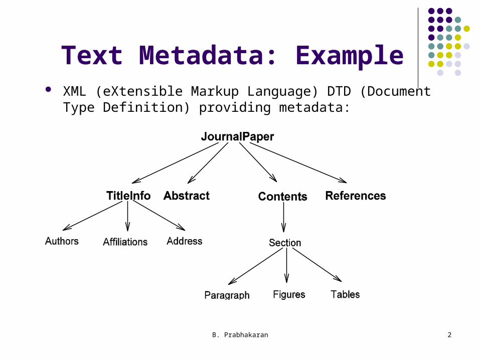
Text Metadata: Example XML (eXtensible Markup Language) DTD (Document Type

Definition) providing metadata:

B. Prabhakaran 3

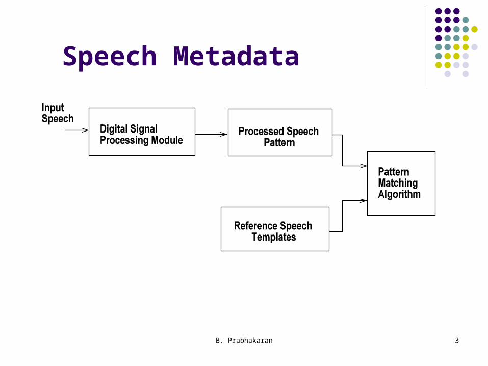
Speech Metadata

B. Prabhakaran 4

Speech Pattern Matching Comparison of a speech sample with a reference

template simple If compared directly, by summing the distances between

respective speech frames. Summation provides overall distance measure of similarity

Complicated by non-linear variations in timing produced from utterance to utterance.

Results in misalignment of the frames of the spoken word with those in the reference template.

B. Prabhakaran 5

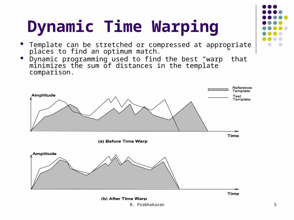
Dynamic Time Warping Template can be stretched or compressed at appropriate

places to find an optimum match. Dynamic programming used to find the best “warp” that

minimizes the sum of distances in the template comparison.

B. Prabhakaran 6

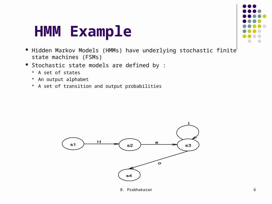
HMM Example Hidden Markov Models (HMMs) have underlying stochastic finite state machines

(FSMs) Stochastic state models are defined by :

A set of states An output alphabet A set of transition and output probabilities

B. Prabhakaran 7

HMM .. Term hidden for this model: due to fact that the actual state of the FSM cannot be observed directly, only

through the alphabets emitted. Probability distribution can be discrete or continuous. For isolated word recognition, each word in the vocabulary has a corresponding HMM. For continuous speech recognition, the HMM represents the domain grammar. This grammar HMM is

constructed from word-model HMMs. HMMs have to be trained to recognize isolated words or continuous speech.

B. Prabhakaran 8

Artificial Neural Networks

B. Prabhakaran 9

Image Metadata Concept of Scene and Objects

Scene: collection of zero or more objects Object: part of a scene E.g., car is an object in a traffic scene

Both scene and objects have visual features: color, texture, shape, location, and relationships among edges (above, below, behind, …)

Question: how can the visual features be (semi-) automatically detected?

B. Prabhakaran 10

Color Histograms

B. Prabhakaran 11

Image Color Color distribution: histogram of intensity values (color “bins” in

X-axis and intensity in Y-axis) (“Good” property) Histograms: invariant to translation, rotation of

scenes/objects. (“Bad” property) Only “global” property, does not describe

specific objects, shapes, etc. Let Q and I be 2 histograms, having N bins in the same order Intersection of the 2 histograms:

∑i =1 N min(Ii, Qi) Normalized intersection

∑i =1 N min(Ii, Qi) / ∑i =1 N Qi

Varies from 0 to 1. Insensitive to changes in image resolution, histogram size, depth, and view point.

B. Prabhakaran 12

Color Histograms Computationally expensive: O(NM), N: no. of

histogram bins; M: no. of images. Reducing search time: reduce N ? “Cluster” the colors? Overcoming “global” property: divide image into sub-

areas; calculate histogram for each of those sub-areas. Increases storage requirements and comparison time (or

number of comparisons)

B. Prabhakaran 13

Image Texture Contrast: Statistical distribution of pixel intensities Coarseness: Measure of “granularity” of texture

Based on “moving” averages: over a window of different sizes, 2k X 2k, 0 < k < 5.

“Moving” average: computing “gray-level” at a pixel location Carrying out the computation in horizontal and vertical directions.

Directionality: “Gradient” vector is calculated at each pixel Magnitude and angle of this vector can be computed for a “small”

array centered on a pixel. Computation for all pixels yields a histogram Flat histogram: non-directional image; Sharp peaks in histograms:

highly directional images.

B. Prabhakaran 14

Image Segmentation Thresholding Technique:

All pixels with gray level at or above a threshold are assigned to object.

Pixels below the threshold fall outside the object. Threshold value influences the boundary position as well as

the overall size of the object. Region Growing Technique:

Proceeds as though the interior of the object grows until their borders correspond with the edges of the objects.

Image divided into a set of tiny regions which may besingle pixel or a set of pixels.

Properties that distinguish the objects (e.g., gray levels, color or texture) are identified

A value for these properties are assigned for each region.

B. Prabhakaran 15

Face Recognition

B. Prabhakaran 16

Video Metadata Generation Identify logical information units in the video Identify different types of video camera

operations Identify the low-level image properties of the

video (such as lighting) Identify the semantic properties of the parsed

logical unit Identify objects and their properties (such as

object motion) in the video frames

B. Prabhakaran 17

Video Shots/Clips Logical unit of video information to be parsed

automatically: camera shot or clip. Shot: a sequence of frames representing a contiguous

action in time and space. Basic idea: frames on either side of a camera break

shows a significant change in the information content. Algorithm needs a quantitative metric to capture the

information content of a frame. Shot identification: whether the difference between the

metrics of two consecutive video frames exceed a threshold.

Gets complex when fancy video presentation techniques such as dissolve, wipe, fade-in or fade-out are used.

B. Prabhakaran 18

Shot Identification Metrics Comparison of corresponding pixels or

blocks in the frame Comparison of histograms based on color

or gray-level

B. Prabhakaran 19

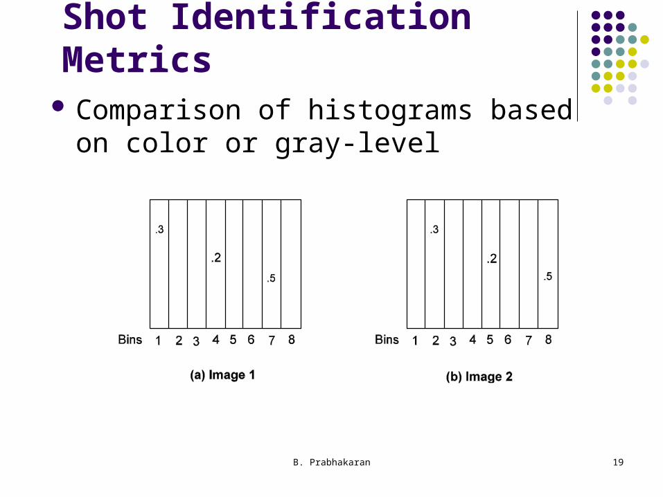
Shot Identification Metrics Comparison of histograms based on color

or gray-level

B. Prabhakaran 20

Algorithms for Uncompressed Video

Histogram Based Algorithm Extracted color features of a video frame are

stored in the form of color bins with the histogram value indicating the percentage (or normalized population) of pixels that are most similar to a particular color.

Each bin: typically a cube in the 3-dimensionalcolor space (corresponding to the basic colors red, green, and blue).

Any two points in the same bin represent the same color.

B. Prabhakaran 21

Algorithms for Uncompressed Video ….

Histogram Based Algorithm … Shot boundaries identified by comparing the

following features between two video frames : gray level sums, gray level histograms, and color histograms.

Here, video frames partitioned into sixteen windows and the corresponding windows in two frames are compared based on the above features.

Division of frames helps in reducing errors due to object motion or camera movements.

Does not consider gradual transition between shots.

B. Prabhakaran 22

Algorithms for Compressed Video Motion JPEG Video

Video frame grouped into data units of 8 * 8 pixels and a Discrete Cosine Transform (DCT) applied to these data units.

DCT coefficients of each frame mathematically related to the spatial domain and hence represents the contents of the frames.

Video shots in motion JPEG identified based on correlation between the DCT coefficients of video frames. Apply a skip factor to select the video frames to be

compared Select regions in the selected frames. Decompress only

the selected regions for further comparison

B. Prabhakaran 23

Selective Video Decoder

B. Prabhakaran 24

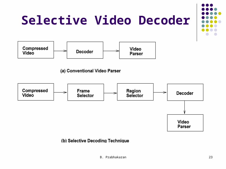
Algorithms for Compressed Video Frame selector uses a skip factor to determine the

subsequent number of frames to be compared. Region selector employs a DCT coefficients based

approach to identify the regions for decompression and for subsequent image processing.

Algorithm adopts a multi-pass approach with the first approach isolating the regions of potential cut points.

Frames that cannot be classified based on DCT coefficients comparison are decompressed for further examination by color histogram approach.

B. Prabhakaran 25

MPEG Video Selection To achieve high rate of compression, redundant

information in the subsequent frames are coded based on the information in the previous frames.

Such frames are termed P and B frames. To provide fast random access, some of the frames are

compressed independently, called I frames. MPEG video stream to be of the following sequence of frames :

IBBPBBPBBIBBPBBP....

B. Prabhakaran 26

Parsing MPEG Video A difference metric for comparison of DCT coefficients

between video frames needed. Difference metric using the DCT coefficients can be

applied only on the I frames of the MPEG video (since only those are coded with DCT coefficients).

Motion information coded in the MPEG data can be used for parsing. Basic idea: B and P frames coded with motion

vectors; the residual error after motion compensation is transformed and coded with DCT coefficients.

Residual error rates are likely to be very high at shot boundaries. Number of motion vectors in the B or P frame is likely to be very few.

B. Prabhakaran 27

Parsing MPEG Video Motion information coded in the MPEG data can be

used for parsing. Algorithm detects a shot boundary if the number of

motion vectors are lower than a threshold value. Can lead to detection of false boundaries

because a shot boundary can lie between two successive I frames.

Advantage is that the processing overhead is reduced as number of I frames are relatively fewer.

Algorithm also does partitioning of the video frames based on motion vectors.

B. Prabhakaran 28

Shots With Transitions Hybrid approach of employing both the DCT coefficient

based comparison and motion vector based comparison.

First step: apply a DCT comparison to I frames with a large skip factor to detect regions of potential gradual transitions.

In the second pass, the comparison is repeated with a smaller skip factor to identify shot boundaries that may lie in between.

Then the motion vector based comparison is applied as another pass on the B and P frames of sequences containing potential breaks and transitions.

This helps in refining and confirming the shot boundaries detected by the shot boundaries.

B. Prabhakaran 29

Camera Operations, Object Motions Induce a specific pattern in the field of motion vectors. Panning and tilting (horizontal or vertical rotation) of the

camera causes the presence of strong motion vectors corresponding to the direction of the camera movement.

Disadvantage (for detection of pan and tilt operations): movement of a large object or a group of objects in the same direction can also result in a similar pattern for the motion vectors.

Motion field of each frame can be divided into a number of macro blocks and then motion analysis can be applied to each block.

B. Prabhakaran 30

Camera Operations, Object Motions .. If the direction of all the macro blocks agree, it is

considered as arising due to camera operation (pan/tilt). Otherwise it is considered as arising due to object motion.

Zoom operation: a focus center for motion vectors is created, resulting in the top and bottom vertical components of motion vectors with opposite signs.

Similarly, leftmost and rightmost horizontal components of the motion vectors will have the opposite sign.

This information is used for identification of zooming operation.

B. Prabhakaran 31

3D Models: Shape-based Retrieval Arizona State University: 3dk.asu.edu CMU: amp.ece.cmu.edu/projects/3DModelRetrieval/ Drexel Univ: www.designrepository.org Heriot-Watt University: www.shaperesearch.net IBM:

www.trl.ibm.com/projects/3dweb/SimSearch_e.htm Informatics & Telematics Inst.: 3d-search.iti.gr/ National Research Council, Canada:

www.cleopatra.nrc.ca Princeton: shape.cs.princeton.edu Purdue: tools.ecn.purdue.edu/~cise/dess.html

B. Prabhakaran 32

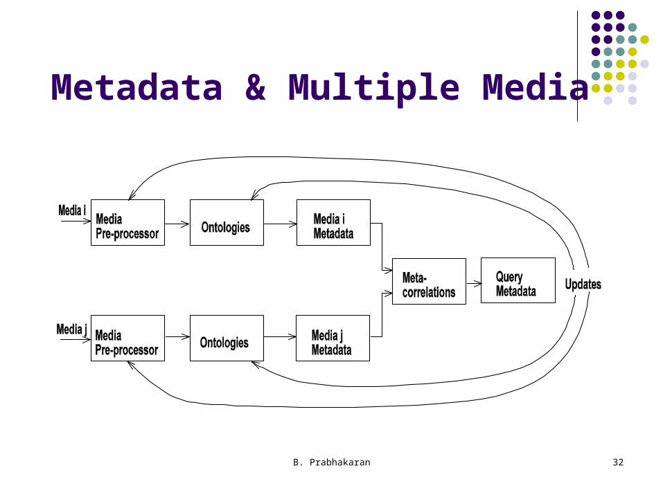
Metadata & Multiple Media