B MUTLU SUMER - Technical University of Denmark · LECTURE NOTES ON TURBULENCE B. MUTLU SUMER...
191
LECT URE NOT ES ON T URBULENCE B. MUTLU SUMER Technical University of Denmark DTU Mekanik, Section for Fluid Mechanics, Coastal & Maritime Engineering Building 403, 2800 Lyngby, Denmark, [email protected] Revised 2013
Transcript of B MUTLU SUMER - Technical University of Denmark · LECTURE NOTES ON TURBULENCE B. MUTLU SUMER...
LECT URE NOT ES ON T URBULENCE
B. MUTLU SUMER
Technical University of Denmark
DTU Mekanik, Section for Fluid Mechanics, Coastal & Maritime Engineering
Building 403, 2800 Lyngby, Denmark, [email protected]
Revised 2013

2

Contents
1 Basic equations 71.1 Method of averaging and Reynolds decomposition . . . . . . . 71.2 Continuity equation . . . . . . . . . . . . . . . . . . . . . . . . 81.3 Equations of motion . . . . . . . . . . . . . . . . . . . . . . . 91.4 Energy equation . . . . . . . . . . . . . . . . . . . . . . . . . . 11
1.4.1 Energy equation for laminar flows . . . . . . . . . . . . 111.4.2 Energy equation for the mean flow . . . . . . . . . . . 121.4.3 Energy equation for the fluctuating flow . . . . . . . . 13
1.5 References . . . . . . . . . . . . . . . . . . . . . . . . . . . . . 15
2 Steady boundary layers 172.1 Flow close to a wall . . . . . . . . . . . . . . . . . . . . . . . . 17
2.1.1 Idealized flow in half space y>0 . . . . . . . . . . . . . 172.1.2 Mean and turbulence characteristics of flow close to a
smooth wall . . . . . . . . . . . . . . . . . . . . . . . . 232.1.3 Mean and turbulence characteristics of flow close to a
rough wall . . . . . . . . . . . . . . . . . . . . . . . . 312.2 Flow across the entire section . . . . . . . . . . . . . . . . . . 432.3 Turbulence-modelling approach . . . . . . . . . . . . . . . . . 48
2.3.1 Turbulence modelling of flow close to a wall . . . . . . 492.3.2 Turbulence modelling of flow across the entire section . 57
2.4 Flow resistance . . . . . . . . . . . . . . . . . . . . . . . . . . 592.5 Bursting process . . . . . . . . . . . . . . . . . . . . . . . . . 612.6 Appendix. Dimensional analysis . . . . . . . . . . . . . . . . . 662.7 References . . . . . . . . . . . . . . . . . . . . . . . . . . . . . 69
3 Statistical analysis 733.1 Probability density function . . . . . . . . . . . . . . . . . . . 73
3

4 CONTENTS
3.2 Correlation analysis . . . . . . . . . . . . . . . . . . . . . . . . 763.2.1 Space correlations . . . . . . . . . . . . . . . . . . . . . 763.2.2 Time correlations . . . . . . . . . . . . . . . . . . . . . 81
3.3 Spectrum analysis . . . . . . . . . . . . . . . . . . . . . . . . . 843.3.1 General considerations . . . . . . . . . . . . . . . . . . 853.3.2 Energy balance in wave number space . . . . . . . . . . 873.3.3 Kolmogoroff’s theory. Universal equilibrium range and
inertial subrange . . . . . . . . . . . . . . . . . . . . . 913.3.4 One-dimensional spectrum . . . . . . . . . . . . . . . . 94
3.4 References . . . . . . . . . . . . . . . . . . . . . . . . . . . . . 98
4 Diffusion and dispersion 994.1 One-Particle analysis . . . . . . . . . . . . . . . . . . . . . . . 99
4.1.1 Diffusion for small times . . . . . . . . . . . . . . . . . 1034.1.2 Diffusion for large times . . . . . . . . . . . . . . . . . 104
4.2 Longitudinal dispersion . . . . . . . . . . . . . . . . . . . . . . 1134.2.1 Mechanism of longitudinal dispersion . . . . . . . . . . 1134.2.2 Application of one-particle analysis . . . . . . . . . . . 114
4.3 Calculation of dispersion coefficient . . . . . . . . . . . . . . . 1184.3.1 Formulation . . . . . . . . . . . . . . . . . . . . . . . . 1194.3.2 Zeroth moment of concentration . . . . . . . . . . . . . 1214.3.3 Mean particle velocity . . . . . . . . . . . . . . . . . . 1234.3.4 Longitudinal dispersion coefficient . . . . . . . . . . . . 124
4.4 Longitudinal dispersion in rivers . . . . . . . . . . . . . . . . . 1264.5 References . . . . . . . . . . . . . . . . . . . . . . . . . . . . . 129
5 Wave boundary layers 1315.1 Laminar wave boundary layers . . . . . . . . . . . . . . . . . . 132
5.1.1 Velocity distribution across the boundary layer depth . 1325.1.2 Flow resistance . . . . . . . . . . . . . . . . . . . . . . 135
5.2 Laminar-to-turbulent transition . . . . . . . . . . . . . . . . . 1365.3 Turbulent wave boundary layers . . . . . . . . . . . . . . . . . 140
5.3.1 Ensemble averaging . . . . . . . . . . . . . . . . . . . . 1405.3.2 Mean flow velocity . . . . . . . . . . . . . . . . . . . . 1415.3.3 Flow resistance . . . . . . . . . . . . . . . . . . . . . . 1445.3.4 Turbulence quantities . . . . . . . . . . . . . . . . . . . 1445.3.5 Effect of Reynolds number . . . . . . . . . . . . . . . . 1445.3.6 Boundary layer thickness . . . . . . . . . . . . . . . . . 146

CONTENTS 5
5.3.7 Turbulent wave boundary layers over rough walls . . . 1485.4 Other aspects . . . . . . . . . . . . . . . . . . . . . . . . . . . 1515.5 References . . . . . . . . . . . . . . . . . . . . . . . . . . . . . 152
6 Turbulence modelling 1556.1 The closure problem . . . . . . . . . . . . . . . . . . . . . . . 1556.2 Turbulence models . . . . . . . . . . . . . . . . . . . . . . . . 1566.3 Mixing-length model . . . . . . . . . . . . . . . . . . . . . . . 157
6.3.1 Turbulent transport of momentum . . . . . . . . . . . 1576.3.2 Mixing length . . . . . . . . . . . . . . . . . . . . . . . 160
6.4 k-omega model . . . . . . . . . . . . . . . . . . . . . . . . . . 1696.4.1 Model equations . . . . . . . . . . . . . . . . . . . . . 1696.4.2 Model constants . . . . . . . . . . . . . . . . . . . . . . 1716.4.3 Blending function F1 . . . . . . . . . . . . . . . . . . . 171
6.4.4 Eddy viscosity and Blending function F2 . . . . . . . . 1726.4.5 Boundary conditions . . . . . . . . . . . . . . . . . . . 1726.4.6 Numerical computation . . . . . . . . . . . . . . . . . . 1746.4.7 An application example . . . . . . . . . . . . . . . . . 175
6.5 Large Eddy Simulation (LES) . . . . . . . . . . . . . . . . . . 1816.5.1 Model equations . . . . . . . . . . . . . . . . . . . . . 1816.5.2 An application example . . . . . . . . . . . . . . . . . 183
6.6 References . . . . . . . . . . . . . . . . . . . . . . . . . . . . . 189
6 CONTENTS

Chapter 1
Basic equations
1.1 Method of averaging and Reynolds de-composition
Themean value of a hydrodynamic quantity, for example, the xi− componentof the velocity, ui, is defined by
ui =1
T
t0+T
t0
ui dt (1.1)
in which t0 is any arbitrary time, and T is the time over which the mean istaken. Clearly T should be sufficiently large to give a reliable mean value.This is called time averaging. There are also other kinds of averaging, such
as ensemble averaging, or moving averaging. We shall adopt the ensemble
Figure 1.1: Time series of ui.
7

8 CHAPTER 1. BASIC EQUATIONS
averaging in the case of wave boundary layers, as will be detailed in Chapter5.The instantaneous value of the velocity ui may be written (see Fig. 1.1)
ui = ui + ui (1.2)
in which ui is called the fluctuating part (or fluctuation) of ui, and ui is itsmean. This is called the Reynolds decomposition. The Reynolds decomposi-tion can be applied to any hydrodynamic quantity.Let f and g be any such quantities (any velocity component, pressure,
etc.). The following relations are known as the Reynolds conditions (here,the overbar denotes the time averaging, Eq. 1.1):
f + g = f + g (1.3)
af = af
a = a∂f
∂s=
∂f
∂s
fg = fg
f = f
f = 0
fg = fg
fh = f h = 0
in which a = constant, and s = x1, x2, x3, t.
1.2 Continuity equation
For an incompressible fluid (such as water), the continuity equation is (fromthe conservation of mass)
∂ui∂xi
= 0 (1.4)
where Einstein’s summation convention is used, namely there is summationover the repeated indices:
∂u1∂x1
+∂u2∂x2
+∂u3∂x3
= 0 (1.5)

1.3. EQUATIONS OF MOTION 9
in which ui is the i−component of the velocity.Averaging (Eq. 1.1) gives:
∂ui∂xi
=∂ui∂xi
= 0 (1.6)
Subtracting the preceding equation from Eq. 1.4 gives
∂ui∂xi
= 0 (1.7)
To sum up, Eq. 1.6 is the continuity equation for the mean velocity andEq. 1.7 is the continuity equation for its fluctuating part.
1.3 Equations of motion
For a Newtonian fluid (such as water) the Navier-Stokes (N.-S.) equation is
ρ(∂ui∂t+ uj
∂ui∂xj
) = ρgi +∂σij∂xj
(1.8)
in which t is the time, gi is the volume force (such as the gravity force) andxi is the Cartesian coordinates. The quantity σij is the stress on the fluid,and given as
σij = −pδij + μ(∂ui∂xj
+∂uj∂xi
) (1.9)
The preceding relation is the constitutive equation for a Newtonian fluid.Here, p is the pressure, and μ is the viscosity, and δij is the Kronecker deltadefined as
δij = 1 for i = j, (1.10)
δij = 0 for i = j
From the continuity equation (Eq. 1.4), the N.-S. equation becomes
ρ∂ui∂t+
∂
∂xj(ρuiuj) = ρgi +
∂σij∂xj
(1.11)
and averaging each term
ρ∂ui∂t+
∂
∂xj(ρuiuj) = ρgi +
∂σij∂xj
(1.12)

10 CHAPTER 1. BASIC EQUATIONS
Now, the second term on the left hand side of the preceding equation (usingthe Reynolds decomposition)
∂
∂xj(ρuiuj) = ρuj
∂ui∂xj
+∂
∂xj(ρuiuj) (1.13)
Inserting the preceding equation in Eq. 1.12
ρ(∂ui∂t+ uj
∂ui∂xj
) = ρgi +∂
∂xj(σij − ρuiuj) (1.14)
This equation is known as the Reynolds equation.As seen, the equation of motion for the mean flow in the case of the
turbulent flow (Eq. 1.14) is quite similar to that in the case of the laminarflow (Eq. 1.8). Comparison of the two equations indicates that, in the caseof the turbulent flow, there is an additional stress, namely −ρuiuj. Thisadditional stress is called the Reynolds stress. There are nine such stresses
−ρuiuj =
⎡⎣ −ρu1u1 − ρu1u2 − ρu1u3−ρu2u1 − ρu2u2 − ρu2u3−ρu3u1 − ρu3u2 − ρu3u3
⎤⎦ (1.15)
As seen, these stresses form a symmetrical second order tensor (the Reynoldsstress tensor).To summarize at this point, there are four equations for the mean flow.
These are
1. the continuity equation (Eq. 1.6) and
2. three equations of motion (Eq. 1.14),
and there are ten unknowns (namely, three components of the velocity,ui, and the pressure, p, and six components of the Reynolds stress, −ρuiuj).Therefore the system is not closed. This problem is known as the closureproblem of turbulence. We shall return to this problem later.(In the case of laminar flow, there are four unknowns (namely, three com-
ponents of the velocity, ui, and the pressure, p) and four equations, namelythe continuity equation (Eq. 1.4) and three N.-S. equation (Eqs. 1.8 and1.9). Therefore, the system is closed.)

1.4. ENERGY EQUATION 11
1.4 Energy equation
1.4.1 Energy equation for laminar flows
N.-S. equation:
∂ui∂t+ uα
∂ui∂xα
= gi −1
ρ
∂p
∂xi+ ν
∂2ui∂xα∂xα
(1.16)
Multiplying both sides of the equation by uj
uj∂ui∂t+ ujuα
∂ui∂xα
= ujgi − uj1
ρ
∂p
∂xi+ νuj
∂2ui∂xα∂xα
(1.17)
The first term on the left hand side is
uj∂ui∂t
=∂
∂t(uiuj)− ui
∂uj∂t
(1.18)
and solving ∂uj∂tfrom Eq. 1.16, and inserting it into the preceding equation
gives
uj∂ui∂t
=∂
∂t(uiuj)− ui(gj −
1
ρ
∂p
∂xj+ ν
∂2uj∂xα∂xα
− uα∂uj∂xα
) (1.19)
Substituting the latter equation in Eq. 1.17, and setting i = j,
∂
∂t(1
2ρuiui) + ui
∂p
∂xi+ ρuiuα
∂ui∂xα
= ρuigi + μui∂2ui
∂xα∂xα(1.20)
Adding the term
−μ( ∂ui∂xα
+∂uα∂xi
)∂ui∂xα
on both sides of the equation and also the term
μui∂2uα
∂xi∂xα
on the right hand side of the equation (this term is actually zero due tocontinuity), and after some algebra, the following equation is obtained
∂K
∂t+
∂
∂xα[Kuα + puα − uiμ(
∂ui∂xα
+∂uα∂xi
)] = ρuαgα − Φ (1.21)

12 CHAPTER 1. BASIC EQUATIONS
in which K is the kinetic energy per unit volume of fluid
K =1
2ρuiui =
1
2ρ(u2 + v2 + w2) (1.22)
and Φ is the energy dissipation per unit volume of fluid and per unit time
Φ = μ(∂ui∂xα
+∂uα∂xi
)∂ui∂xα
(1.23)
1.4.2 Energy equation for the mean flow
The equation of motion for the mean flow (the Reynolds equation, Eq.1.14):
ρ∂ui∂t+ ρuα
∂ui∂xα
= ρgi −∂p
∂xj+ μ
∂2ui∂xα∂xα
+∂
∂xα(−ρuiuα) (1.24)
Now, in the preceding subsection, the energy equation, Eq. 1.21, is ob-tained from the equation of motion, Eq. 1.16. In a similar manner, the energyequation for the mean flow can be obtained from the equation of motion forthe mean flow (i.e., from Eq. 1.24). The result is
∂K0
∂t+
∂
∂xα[K0uα+ρuiuαui+p uα−uiμ(
∂ui∂xα
+∂uα∂xi
)] = ρuαgα−Φ0−(−ρuiuα)∂ui∂xα
(1.25)in which K0 is the kinetic energy per unit volume of fluid for the mean flow
K0 =1
2ρuiui =
1
2ρ(u2 + v2 + w2) (1.26)
and Φ0 is the energy dissipation per unit volume of fluid and per unit time,again, for the mean flow
Φ0 = μ(∂ui∂xα
+∂uα∂xi
)∂ui∂xα
(1.27)
Now, note the last term on the right hand side of Eq. 1.25. We shall returnto this term in the next subsection.
1.4. ENERGY EQUATION 13
1.4.3 Energy equation for the fluctuating flow
Averaging Eq. 1.21 gives
∂
∂t(1
2ρuiui) +
∂
∂xα[1
2ρuiuiuα + puα − uiμ(
∂ui∂xα
+∂uα∂xi
)] = ρuαgα −Φ (1.28)
Furthermore, Eq. 1.25:
∂
∂t(1
2ρuiui) +
∂
∂xα[1
2ρuiuαui + ρuiuαui + p uα − uiμ(
∂ui∂xα
+∂uα∂xi
)] =
= ρuαgα − Φ0 − (−ρuiuα)∂ui∂xα
(1.29)
Subtracting Eq. 1.29 from Eq. 1.28 gives
∂Kt
∂t+
∂
∂xα[Ktuα+
1
2ρuiuiuα+p uα−uiμ(
∂ui∂xα
+∂uα∂xi
)] = ρuαgα−Φt+(−ρuiuα)∂ui∂xα
(1.30)in which Kt is the kinetic energy per unit volume of fluid for the fluctuatingflow (i.e., the kinetic energy of turbulence)
Kt =1
2ρuiui =
1
2ρ(u 2 + v 2 + w 2) (1.31)
and Φt is the viscous dissipation of the turbulent energy per unit volume offluid and per unit time
Φt = μ(∂ui∂xα
+∂uα∂xi
)∂ui∂xα
(1.32)
Eq. 1.25 is the energy equation for the mean flow, and Eq.1.30 is thatfor turbulence. As seen, the term (−ρuiuα) ∂ui∂xα
is common in both equations,but with opposite signs. This implies that if this term is an energy gain forturbulence, then it will be an energy loss for the mean flow, or vice versa.Now, we shall show that this term is an energy gain for turbulence.Integrating Eq.1.30 over a volume V gives
∂
∂t V
Kt dV+S
Fαnα dS =V
ρuαgα dV−V
Φt dV+V
(−ρuiuα)∂ui∂xα
dV
(1.33)

14 CHAPTER 1. BASIC EQUATIONS
in which
Fα = Ktuα +1
2ρuiuiuα + p uα − uiμ(
∂ui∂xα
+∂uα∂xi
) (1.34)
and S is the surface encircling the volume V. Here, the volume integral inthe second term on the left hand side of Eq. 1.33 is converted to a surfaceintegral, using the Green-Gauss theorem. The first term on the right handside of Eq. 1.33 drops when the volume force is taken as the gravity force,since gα = 0. The second term on the left hand side of Eq. 1.33, on the otherhand, is the energy flux at the surface S. Therefore, it is not a source term.Now, consider a situation where there is no influx of turbulent energy. Inthis case, the maintenance of turbulence (i.e., ∂
∂t VKt dV ≥ 0 in Eq. 1.33) is
only possible whenV(−ρuiuα) ∂ui∂xα
dV in Eq. 1.33 is positive, meaning thatthe term (−ρuiuα) ∂ui∂xα
in the turbulence energy equation (Eq. 1.30) shouldbe positive. In other words, this term is an energy gain for turbulence, andtherefore it is an energy loss for the mean flow. This is an important result,because it implies that turbulence extracts its energy from the mean flow, andthe rate at which the energy is extracted from the mean flow is (−ρuiuα) ∂ui∂xα
.An important implication of the above result is that turbulence is gen-
erated only when there exists a velocity gradient in the flow ∂ui∂xα. When
there is no velocity gradient, no turbulence will be generated. In this case,any field of turbulence introduced into the flow will be dissipated (the de-cay of turbulence). See Monin and Yaglom (1973, pp. 373-388) for furtherdiscussion.
Example 1 Find the turbulence energy generation and the total energy dis-sipation (per unit volume of fluid and per unit time) for a turbulent boundaryflow in an open channel (Fig. 1.2).
The energy extracted from the mean flow is (−ρuiuα) ∂ui∂xα. For the present
flow, this will be
(−ρu v )∂u∂y
This is the energy extracted from the mean flow per unit time and per unitvolume of fluid (Fig. 1.2 c). As seen from the figure, the energy ”generation”for turbulence is zero at the free surface while it increases tremendously asthe wall is approached.

1.5. REFERENCES 15
Figure 1.2: (a) Shear stress, (b) velocity and (c) turbulent energy extracted fromthe mean flow.
From Eq. 1.25, the total energy dissipation, on the other hand, is
Φ0 + (−ρuiuα)∂ui∂xα
in which Φ0 is given in Eq. 1.27. The total energy dissipation will thereforebe
(μ∂u
∂y)∂u
∂y+ (−ρu v )∂u
∂y
From the preceding relation, it is seen that the energy dissipation is verylarge near the wall, and it decreases with the distance from the wall, similarto the variation of the turbulent energy generation (Fig. 1.2 c).
1.5 References
1. Monin, A.S. and Yaglom, A.M. (1973). Statistical Fluid Mechanics:Mechanics of Turbulence, vol. 1, MIT Press. Cambridge, Mass.

16 CHAPTER 1. BASIC EQUATIONS
Chapter 2
Steady boundary layers
In this chapter, we will study steady, turbulent boundary layers over a wall,in a channel, or in a pipe. (Examples of turbulent boundary layers over awall may be: flow over a flat plate, flow over the seabed, the atmosphericboundary-layer flow over the earth surface, etc.).We will first concentrate on the flow close to a wall (a general analysis),
and then we will study the flow close to a smooth wall, and subsequentlythat close to a rough wall. (The latter will include the flow near the bedof a channel, and that near the wall of a pipe, etc.). Finally, we will turnour attention to flows in channels/pipes, considering the entire channel/pipecross section.
2.1 Flow close to a wall
2.1.1 Idealized flow in half space y>0
First, consider the following idealized case.The flow is steady, and takes place in the half space y > 0 (Fig. 2.1),
and there is no pressure gradient in the horizontal direction, i.e., no pressuregradient in the x− direction.Shear stress.
The basic equations are the continuity equation and the two componentsof the Reynolds equation. The continuity equation is automatically satis-fied. The y− component of the Reynolds equation gives an equation for the
17

18 CHAPTER 2. STEADY BOUNDARY LAYERS
Figure 2.1: Shear stress in the idealized half space y > 0.
Reynolds stress −ρv 2. The x− component of the Reynolds equation (Eq.1.14), on the other hand, reads
ρ(∂u
∂t+ u
∂u
∂x+ v
∂u
∂y) = ρgx−
∂p
∂x+μ(
∂2u
∂x2+
∂2u
∂y2) +
∂
∂x(−ρu 2) + ∂
∂y(−ρu v )
(2.1)Since ∂u
∂t= 0, v = 0, gx = 0,
∂p∂x= 0, u is a function of only y, and the flow is
uniform in the x− direction (i.e., ∂u∂x= 0), then the Reynolds equation will
be
μd2u
dy2+d
dy(−ρu v ) = 0 (2.2)
or,d
dy(μdu
dy+ (−ρu v )) = dτ
dy= 0 (2.3)
in which τ is the total shear stress:
τ = μdu
dy+ (−ρu v ) (2.4)
which is composed of two parts, namely the viscous part (the first term), andthe part induced by turbulence (the Reynolds stress, the second term).Integrating 2.3 gives
τ = c; c = constant (2.5)
The boundary condition at the wall:
y = 0 : τ = τ 0 (2.6)

2.1. FLOW CLOSE TO A WALL 19
in which τ 0 is the wall shear stress. From Eqs. 2.4 and 2.6, one obtains
τ(= μdu
dy+ (−ρu v )) = τ 0 (2.7)
This is an important result. It shows that the shear stress is constantover the entire depth, and equal to the wall shear stress, τ 0.
Mean velocity.Our objective is to determine the velocity u as a function of y. To this end,
we resort to dimensional analysis (see Appendix at the end of this chapterfor a brief account of the dimensional analysis).Now, the mean properties of the flow (such as u) depend on the following
quantitiesτ 0, y, μ, ρ (2.8)
Here we consider a smooth wall, therefore no parameter representing the wallroughness is included.The flow depends on τ 0 because the shear stress determines the flow
velocity; the larger the shear stress, the larger the flow velocity. (Also, it mustbe stressed that the shear stress in this idealized case remains unchangedacross the depth, as shown in the preceding paragraphs).Likewise, the flow depends on the distance from the wall, y, because the
closer to the wall, the smaller the velocity (just at the wall, obviously thevelocity will be zero due to the no-slip condition).Clearly, the flow should also depend on the fluid properties, namely μ,
and ρ.Hence
u = F (τ 0, y, μ, ρ) (2.9)
orΦ(u, τ 0, y, μ, ρ) = 0 (2.10)
From dimensional analysis, the preceding dimensional function Φ can beconverted to a nondimensional function φ
φ(u
Uf,yUfν) = 0 (2.11)
in which uUf, and yUf
νare two nondimensional quantities, Uf is the friction
velocity defined by
Uf =τ 0ρ
(2.12)

20 CHAPTER 2. STEADY BOUNDARY LAYERS
Figure 2.2: Flow in an open channel.
and ν is the kinematic viscosity
ν =μ
ρ(2.13)
Solving uUffrom Eq. 2.11
u
Uf= f(y+) (2.14)
in whichy+ =
yUfν
(2.15)
Eq. 2.14 is known as the law of the wall. The quantities Uf and ν are calledthe inner flow parameters, or wall parameters.
Example 2 Boundary layer in an open channel. Flow close to the bed ofthe channel.
Now, consider a real-life flow, namely the flow in an open channel (Fig.2.2). The flow in the channel is driven by gravity, with the volume forcegx = gS in which S is the slope of the channel. The x− component of theReynolds equation, Eq. 2.3, will in the present case read
d
dy(μdu
dy+ (−ρu v )) = dτ
dy= −ρgx = −ρgS = −γS (2.16)
in which γ is the specific weight of the fluid. Integrating gives
τ = −γSy + c; c: constant (2.17)

2.1. FLOW CLOSE TO A WALL 21
The boundary condition at the free surface:
y = h : τ = 0 (2.18)
which gives c = γSh where h is the depth. Then the shear stress
τ = γSh(1− yh) (2.19)
The wall shear stress (the bed shear stress) will then be
τ 0 = γSh (2.20)
Hence, the shear stressτ = τ 0(1−
y
h) (2.21)
(see sketch in Fig. 2.2).Our main concern in this section is the flow close to the wall. Close to
the wall, i.e., y h, the wall shear stress
τ = τ 0(1−y
h) τ 0 (2.22)
i.e., near the wall, the shear stress can be assumed to be constant and equalto the wall shear stress, τ τ 0. This thin layer of fluid is called the constantstress layer.As seen, the flow in the constant stress layer is similar to the idealized
flow considered in the preceding section; in both flows, the shear stress isconstant across the depth. The immediate implication of this result is that,the velocity distribution close to the wall in the present case (i.e., in theconstant stress layer) is given by the law of the wall (Eq. 2.14):
u
Uf= f(y+) (2.23)
Example 3 Boundary layer in a pipe. Flow close to the wall of the pipe.
Now, consider a fully developed turbulent boundary layer in a pipe (Fig.2.3).Similar to the previous example, the x− component of the Reynolds equa-
tion in the present case:1
r
∂
∂r(rτ) =
∂p
∂x(2.24)

22 CHAPTER 2. STEADY BOUNDARY LAYERS
Figure 2.3: Flow in a pipe.
Here, the gravity term is included in the pressure gradient term for conve-nience. The flow is driven by the pressure gradient ∂p
∂x.
Integrating Eq.2.24 gives
rτ =∂p
∂x
r2
2+ c (2.25)
in which c is a constant.The boundary condition at the center line of the pipe
r = 0 : τ = 0 (2.26)
which gives c = 0. The boundary condition at the wall of the pipe
r =D
2: τ = τ 0 (2.27)
From Eqs.2.25 and 2.27, one gets
τ = 2τ 0r
Dor τ = τ 0(1−
2y
D) (2.28)
in which y = D2− r is the distance from the pipe wall.
Again, similar to the previous example, for y D2, i.e., close to the wall,
the shear stress can be assumed to be constant and approximately equalto the wall shear stress τ τ 0, the constant stress layer. Similar to theboundary layer in an open channel, in this thin layer of fluid near the wallof the pipe, the velocity is given by the law of the wall
u
Uf= f(y+) (2.29)

2.1. FLOW CLOSE TO A WALL 23
2.1.2 Mean and turbulence characteristics of flow closeto a smooth wall
In this subsection, mean and turbulence characteristics of the boundary layerflow close to a wall will be studied in greater detail. As seen in the previ-ous examples, the shear stress near the wall is approximately constant, andcan be taken equal to the wall shear stress (the constant stress layer). Thissubsection is concerned with the flow in the constant stress layer. The analy-sis regarding the mean velocity will be undertaken for two extreme cases:namely, for small values of y+, and for large values of y+.
Figure 2.4: Shear stress distribution in open channel. Grass (1971).
Mean velocity for small values of y+. Viscous sublayer.As seen in the preceding paragraphs, the total shear stress is composed
of two parts, the viscous part and the turbulent part (Reynolds stress) (Eq.2.4). Fig. 2.4 shows the contribution of each part to the total shear stressas a function of the distance from the wall. The figure indicates that, verynear the wall, the turbulent part is small compared with the viscous part,(−ρu v ) μdu
dy. Hence
τ = τ 0 = μdu
dy+ (−ρu v ) μ
du
dy(2.30)
24 CHAPTER 2. STEADY BOUNDARY LAYERS
or
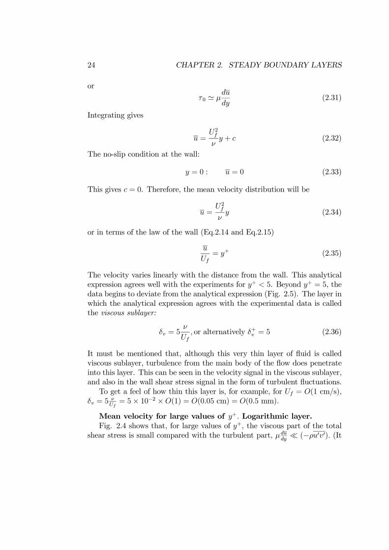
τ 0 μdu
dy(2.31)
Integrating gives
u =U2fνy + c (2.32)
The no-slip condition at the wall:
y = 0 : u = 0 (2.33)
This gives c = 0. Therefore, the mean velocity distribution will be
u =U2fνy (2.34)
or in terms of the law of the wall (Eq.2.14 and Eq.2.15)
u
Uf= y+ (2.35)
The velocity varies linearly with the distance from the wall. This analyticalexpression agrees well with the experiments for y+ < 5. Beyond y+ = 5, thedata begins to deviate from the analytical expression (Fig. 2.5). The layer inwhich the analytical expression agrees with the experimental data is calledthe viscous sublayer:
δv = 5ν
Uf, or alternatively δ+v = 5 (2.36)
It must be mentioned that, although this very thin layer of fluid is calledviscous sublayer, turbulence from the main body of the flow does penetrateinto this layer. This can be seen in the velocity signal in the viscous sublayer,and also in the wall shear stress signal in the form of turbulent fluctuations.To get a feel of how thin this layer is, for example, for Uf = O(1 cm/s),
δv = 5νUf= 5× 10⁻² ×O(1) = O(0.05 cm) = O(0.5 mm).
Mean velocity for large values of y+. Logarithmic layer.Fig. 2.4 shows that, for large values of y+, the viscous part of the total
shear stress is small compared with the turbulent part, μdudy
(−ρu v ). (It

2.1. FLOW CLOSE TO A WALL 25
should be noted that, although y+ is large, yet y is still small compared withh so that τ τ 0, namely y is in the constant stress layer).Now, the shear stress generates the velocity variation over the depth; i.e.,
the cause-and-effect relationship between the shear stress τ and the velocityvariation du
dyis such that τ generates du
dy.
Since the shear stress for large values of y+ is practically uninfluencedby the viscosity, the velocity variation du
dyshould also be uninfluenced by the
viscosity; therefore, dropping the viscosity μ, from Eq. 2.9,
du
dy=d
dyF (τ 0, y, ρ) (2.37)
or
Ψ(du
dy, τ 0, y, ρ) = 0 (2.38)
From dimensional analysis, this dimensional equation is converted to thefollowing nondimensional equation:
ψ(du
dy
1Ufy
) = 0 (2.39)
This equation has a single variable, namely
du
dy
1Ufy
Solving this variable from Eq. 2.39 will give
du
dy
1Ufy
= A (2.40)
in which A is a constant (the solution).Integrating Eq. 2.40 gives
u = AUf ln y + B1 (2.41)
or in terms of the law of the wall (Eq.2.14 and Eq.2.15):
u = Uf (A ln y+ + B) (2.42)
in which B is another constant. This expression is known as the logarithmiclaw.

26 CHAPTER 2. STEADY BOUNDARY LAYERS
Figure 2.5: Velocity distribution. Taken from Monin and Yaglom (1973).
1. Experiments done in pipe flows, in channel flows, and in boundary layerflows over walls, etc. have all confirmed the logarithmic law with
A = 2.5, B = 5.1 (2.43)
Constant A is also written in the literature in the form of 1/κ, inwhich κ is called von Karman constant, κ = 0.4. Apparently, A is auniversal constant; no matter what the category of the wall is (smooth,rough, transitional), this constant always assumes the same value, i.e.,A = 2.5, as will be demonstrated later in the section.
2. Fig. 2.5 compares the logarithmic law with the experimental data.It is seen that the logarithmic law agrees quite well with the data inthe range 30 < y+ < 500. (It may be noted, however, that the upper

2.1. FLOW CLOSE TO A WALL 27
bound of the latter interval is related to the flow-depth (boundary-layerthickness) effect; Obviously, this bound is determined by the conditiony h, or alternatively y+ hUf
ν. Hence, depending on the Reynolds
number hUfν, the numerical value of the upper bound may change).
3. The layer in which the logarithmic law is satisfied is called the logarith-mic layer.
4. The lower bound of the logarithmic layer is often taken as y+ = 70 inthe literature. The layer of fluid which lies between the viscous sublayerand the logarithmic layer is called the buffer layer, 5 < y+ < 70.Clearly, in this layer, both the viscous effects and the turbulence effectsare equally important.
The above analysis implies that, for the velocity distribution to satisfythe logarithmic law, the following two conditions have to be met:
1. y should be in the constant stress layer, τ τ 0, and for this
y h
in which h is the flow depth in the case of the open channel flow, orit is the radius in the case of the pipe flow, or the boundary-layerthickness in the case of the boundary layer over a wall. (The abovecondition can be taken as y < 0.1h. However, the data given in Monin& Yaglom (1971, p. 288-289) implies that it can be relaxed even to y <(0.2− 0.3)h);
2. y should be sufficiently large so that the variation of the velocity, dudy,
is independent of the viscosity. For this, y+ should be
y+ > 30− 70
These conditions are to be observed when fitting the logarithmic law(Eq. 2.42) to a measured velocity distribution.
Turbulence quantities.By ”turbulence quantities”, we mean the Reynolds stresses, namely
−ρuiuj =
⎡⎣ −ρu 2 − ρu v − ρu w
−ρv u − ρv 2 − ρv w
−ρw u − ρw v − ρw 2
⎤⎦ (2.44)
28 CHAPTER 2. STEADY BOUNDARY LAYERS
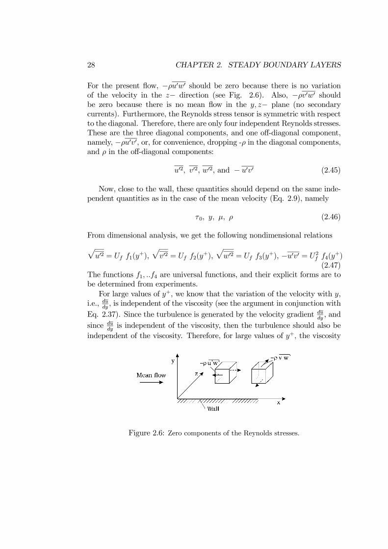
For the present flow, −ρu w should be zero because there is no variationof the velocity in the z− direction (see Fig. 2.6). Also, −ρv w shouldbe zero because there is no mean flow in the y, z− plane (no secondarycurrents). Furthermore, the Reynolds stress tensor is symmetric with respectto the diagonal. Therefore, there are only four independent Reynolds stresses.These are the three diagonal components, and one off-diagonal component,namely, −ρu v , or, for convenience, dropping -ρ in the diagonal components,and ρ in the off-diagonal components:
u 2, v 2, w 2, and − u v (2.45)
Now, close to the wall, these quantities should depend on the same inde-pendent quantities as in the case of the mean velocity (Eq. 2.9), namely
τ 0, y, μ, ρ (2.46)
From dimensional analysis, we get the following nondimensional relations
u 2 = Uf f1(y+), v 2 = Uf f2(y
+), w 2 = Uf f3(y+), −u v = U2f f4(y+)
(2.47)The functions f1, ..f4 are universal functions, and their explicit forms are tobe determined from experiments.For large values of y+, we know that the variation of the velocity with y,
i.e., dudy, is independent of the viscosity (see the argument in conjunction with
Eq. 2.37). Since the turbulence is generated by the velocity gradient dudy, and
since dudyis independent of the viscosity, then the turbulence should also be
independent of the viscosity. Therefore, for large values of y+, the viscosity
Figure 2.6: Zero components of the Reynolds stresses.
2.1. FLOW CLOSE TO A WALL 29
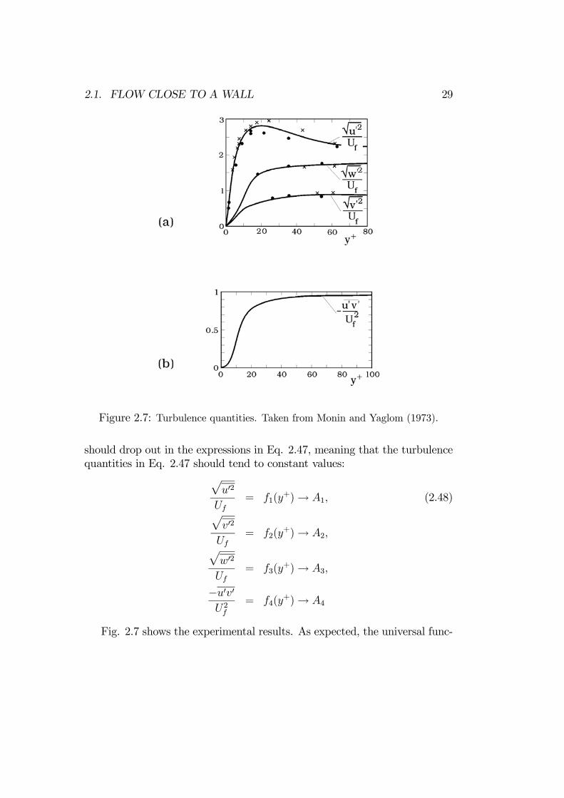
Figure 2.7: Turbulence quantities. Taken from Monin and Yaglom (1973).
should drop out in the expressions in Eq. 2.47, meaning that the turbulencequantities in Eq. 2.47 should tend to constant values:
u 2
Uf= f1(y
+)→ A1, (2.48)
v 2
Uf= f2(y
+)→ A2,
w 2
Uf= f3(y
+)→ A3,
−u vU2f
= f4(y+)→ A4
Fig. 2.7 shows the experimental results. As expected, the universal func-
30 CHAPTER 2. STEADY BOUNDARY LAYERS
tions f1, ..f4 approach zero, as y+ goes to zero, and also, in conformity withEqs. 2.48, they tend to constant values as y+ takes very large values. Fromthe figure, the latter constant values are
A1 2.3, A2 0.9, A3 1.7, and A4 1 (2.49)
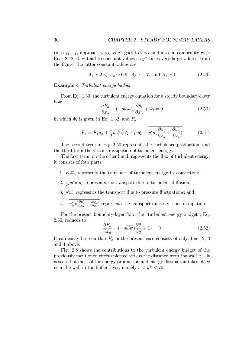
Example 4 Turbulent energy budget
From Eq. 1.30, the turbulent energy equation for a steady boundary-layerflow
∂Fα∂xα− (−ρuiuα)
∂ui∂xα
+ Φt = 0 (2.50)
in which Φt is given in Eq. 1.32, and Fα
Fα = Ktuα +1
2ρuiuiuα + p uα − uiμ(
∂ui∂xα
+∂uα∂xi
) (2.51)
The second term in Eq. 2.50 represents the turbulence production, andthe third term the viscous dissipation of turbulent energy.The first term, on the other hand, represents the flux of turbulent energy;
it consists of four parts:
1. Ktuα represents the transport of turbulent energy by convection;
2. 12ρuiuiuα represents the transport due to turbulent diffusion;
3. p uα represents the transport due to pressure fluctuations; and
4. −uiμ(∂ui∂xα
+ ∂uα∂xi) represents the transport due to viscous dissipation.
For the present boundary-layer flow, the ”turbulent energy budget”, Eq.2.50, reduces to
∂Fα∂xα− (−ρu v )∂u
∂y+ Φt = 0 (2.52)
It can easily be seen that Fα in the present case consists of only items 2, 3and 4 above.Fig. 2.8 shows the contributions to the turbulent energy budget of the
previously mentioned effects plotted versus the distance from the wall y+. Itis seen that most of the energy production and energy dissipation takes placenear the wall in the buffer layer, namely 5 < y+ < 70.

2.1. FLOW CLOSE TO A WALL 31
Figure 2.8: Turbulent energy budget. Laufer (1954).
2.1.3 Mean and turbulence characteristics of flow closeto a rough wall
Mean velocity.Consider that the wall is now covered with roughness elements (Fig. 2.9).
Let the height of the roughness elements be k. Assume that k is sufficientlylarge (larger than the thickness of the viscous sublayer) so that it influencesthe flow.In this case, there is one additional parameter to describe the flow, namely
the roughness height, k. Therefore, Eq. 2.9 will read
u = F (τ 0, y, μ, ρ, k) (2.53)
Now, the total shear stress is given as in the case of the smooth wall (Eq.

32 CHAPTER 2. STEADY BOUNDARY LAYERS
Figure 2.9: Rough wall.
2.4), namely
τ = μdu
dy+ (−ρu v ) (2.54)
However, the turbulent part of the total shear stress, −ρu v , will in thepresent case, consist of two parts:
1. one is induced by the mean velocity gradient, dudy, (in the same way as
in the case of the smooth wall); and
2. the other is caused by the vortex shedding from the roughness elements.(Observations show that lee-wake vortices are shed from the roughnesselements into the main body of the flow in a continuous manner, Sumeret al., 2001).
Clearly, for large distances from the wall, (1) the viscous part μdudyin
the total shear stress (Eq. 2.54) is negligible, as discussed in the previoussection, and (2) the vortex-shedding-induced part of −ρu v is also negligible,because the vortices shed into the flow cannot penetrate to large distancesdue to their limited life time. This means that, for large distances from thewall, the shear stress is practically independent of the viscosity and the wallroughness.Now, as discussed in the previous section, in the cause-and-effect rela-
tionship between the shear stress and the velocity variation, the shear stressis the cause and the velocity variation du
dyis the effect. Since the shear stress
for large distances from the wall is independent of the viscosity and the wall

2.1. FLOW CLOSE TO A WALL 33
roughness, then the velocity variation dudyshould also be independent of these
effects. Hence, dropping out these quantities (i.e., μ and k) in Eq. 2.53,
du
dy=d
dyF (τ 0, y, ρ) (2.55)
This is precisely the same equation as in the case of the smooth wall (Eq.2.37). Therefore, the result obtained in conjunction with Eq. 2.37 is directlyapplicable (Eq. 2.41), i.e.,
u = AUf ln y + B1 (2.56)
Here, A is the same constant as that in the case of the smooth wall, A =2.5. Our analysis implies that this constant has the same value, irrespectiveof the category of the wall (smooth, or rough). Therefore, A must be auniversal constant.In the present context, the preceding expression may be written as
u = AUf ln(y
y0) (2.57)
in which y0 is called the roughness length (not to be confused with the rough-ness height k). Eq. 2.53 suggests that this new quantity should be a functionof μ, k, τ 0 and ρ,
y0 = y0(μ, k, τ 0, ρ) (2.58)
and from dimensional analysis,
y0 = k g(kUfν) (2.59)
The explicit form of the function g(kUfν) can be found from experiments.
Nikuradse carried out such experiments (see Schlichting, 1979); He coatedthe walls of circular pipes with sand grains of given size. The sand grainswere glued on the wall in a densely packed manner. The height of Nikuradse’ssand roughness will be denoted by ks.Changing k by ks, Eq. 2.59 will be
y0 = ks g(ksUfν) (2.60)
According to Nikuradse’s experiments, there are three categories of wall:

34 CHAPTER 2. STEADY BOUNDARY LAYERS
1. Hydraulically smooth wall when ksUfν< 5. (This is when the roughness
height is smaller than the thickness of the viscous sublayer, Eq. 2.36.Clearly, in this case, the roughness elements are covered by the viscoussublayer, and therefore not directly exposed to the main body of theflow. Hence, the wall, although it is rough, acts as a smooth wall);
2. Completely rough wall when ksUfν> 70. (In this case, the viscous sub-
layer is completely destructed, and the roughness elements are com-pletely exposed to the main body of the flow); and
3. Transitional wall when 5 < ksUfν< 70.
Now, in the case of the hydraulically smooth wall, the function g takesthe following form
g(ksUfν) =
aksUfν
(2.61)
This is because ks will drop out only when g is given in the form depictedin the preceding equation. Here a is a constant. Inserting the precedingexpression into Eq. 2.60
y0 = ksa
ksUfν
and from Eq. 2.57
u = AUf ln(y
y0) = AUf ln(
yaUfν
) = AUf ln(1
a
yUfν)
Comparing the preceding equation with Eqs. 2.42 and 2.43 gives the constanta as 1/9.In the case of the completely rough wall, on the other hand, the func-
tion g is given as
g(ksUfν) = b (2.62)
This is because the viscosity does not play any role, and therefore shoulddrop out of formulation; and this is possible only when g is given as in thepreceding form. Here, b is another constant. Nikuradse’s experiments showthat this constant is
g(ksUfν) = b =
1
30(2.63)

2.1. FLOW CLOSE TO A WALL 35
Figure 2.10: Velocity distribution. Rough wall. Grass (1971).
Substituting this into Eq. 2.60, the roughness length will be found
y0 =ks30
(2.64)
and from Eq. 2.57
u = AUf ln(30y
ks) (2.65)
This is the logarithmic law for flow over a completely rough wall. Fig. 2.10compares the above expression with the experimental data (Grass, 1971, Fig.4). As seen, the logarithmic law begins to deviate from the measured velocityprofile for y 0.2ks. This is not unexpected, because it has been seen that,for the velocity profile to satisfy the logarithmic law, y should be sufficientlylarge, so large that the variation of the velocity du
dyis independent of the
wall roughness; otherwise, the velocity distribution will clearly not satisfythe logarithmic law, as revealed by Fig. 2.10.In the case of the transitional wall, the function g is given in Fig. 2.11.
The data can be represented by the following empirical expression:
g(k+s ) =1/9
k+s+1
30exp[−140(k+s + 6)−1.7]

36 CHAPTER 2. STEADY BOUNDARY LAYERS
Figure 2.11: Variation of function g(k+s ). Data: Nikuradse (1933), reproducedfrom Monin and Yaglom (1973). Solid curve: g(k+s ) =
1/9
k+s+ 1
30exp[−140(k+s +
6)−1.7]
Nikuradse’s equivalent sand roughness.The wall roughness is influenced by various factors such as the height of
the roughness elements, the shape of the roughness elements, and the packingpattern. Therefore, it will differ from that in Nikuradse’s experiments. To beable to compare the results obtained with different wall roughnesses, we needa common ”base line”. The concept Nikuradse’s equivalent sand roughnessfacilitates this.The idea is to find Nikuradse’s equivalent sand roughness for any wall
roughness. Nikuradse’s equivalent sand roughness, ks, is defined such thatthe velocity distribution across the depth is given by Eq. 2.65. In practice,it is easy to find ks; the measured velocity distribution is plotted on a semi-logarithmic diagram, and the y− intercept of the line which represents thelogarithmic law (Eq. 2.65) will be ks
30.
The values of Nikuradse’s equivalent sand roughness are reported in theliterature for various wall roughnesses, and they are generally in the rangeks=(2−4)k (Kamphuis, 1974, and the review in the paper by Bayazit, 1983).It may be noted that the upper bound of the previously mentioned range can

2.1. FLOW CLOSE TO A WALL 37
sometimes reach values as much as 5k and even more, depending on the shapeof the roughness elements, the packing pattern as well as the roughness-height-to-flow-depth ratio (the latter is for large values of this ratio such as> O(0.3)) (Bayazit, 1983). In particular, ks=2k for walls covered by sand,pebbles, or stones the size in the range 0.54-46 mm (Kamphuis, 1974); andks=(3− 6)k for the ground covered with ordinary grass or agricultural crops(Monin and Yaglom, 1973). Bayazit (1983) reports the following values forthe equivalent sand roughness for various boundaries:
Author Roughness ks
Leopold et al. (1964) Gravel 3.5D84Limerinos (1970) Gravel 3.5D84Bayazit (1976) Closely packed spheres 2.5DCharlton et al. (1978) Gravel 3.5D90Hey (1979) Gravel 3.5D84Thompson and Campbell (1979) Gravel 4.5D90Gladki (1979) Gravel 2.5D80Denker (1980) Closely-packed cylinders 2DBray (1980) Gravel 3.5D84 (3.1D90)Griffths (1981) Gravel 5D50
Figure 2.12: Theoretical wall.
Finally, ks=2.5k for a river bed where the sediment grains are in motion(k being the grain size). This is when the bed remains plane (i.e., no bedforms are developed) (Engelund and Hansen, 1967). This corresponds to aweak sediment transport, and before bed ripples emerge. When the bed is
38 CHAPTER 2. STEADY BOUNDARY LAYERS
covered with ripples, ks is found to be ks=(2−3)k with 2-D ripples (Fredsøe etal., 2000), k being the ripple height. In the case of 3-D ripples, the previousrelation can, to a first approximation, be used. For very high velocities,ripples are washed away and the bed becomes plane again; This sediment-transport regime is called the sheet-flow regime (Sumer et al., 1996). In thiscase, the ks value can be calculated from the following empirical relations(Sumer et al., 1996):
1. No-suspension sediment transport (w/Uf > 0.8− 1):
ksk= 2 + 0.6θ2.5; 0 < θ 2 (2.66)
2. Suspension sediment transport (w/Uf < 0.8− 1):
ksk= 4.5 +
1
8exp 0.6(
w
Uf)4θ2 θ2.5 (2.67)
in which k is the sediment grain size, w the fall velocity of sedimentgrains and θ the Shields parameter defined by
θ =U2f
g(s− 1)k (2.68)
in which s is the specific gravity of sediment grains and g the acceler-ation due to gravity.
Theoretical wall.In the case of the rough wall, the exact location of the wall is not well
defined. Does it lie at the top of the roughness elements, or does it lie atthe base bottom, or does it lie somewhere between? This issue brings in theconcept of the theoretical wall.Formally, the theoretical wall is defined as the location from which the y
distances in Eq. 2.65 are measured (Fig. 2.12).Now, for convenience, change the coordinate to y , the distance from the
base wall. Now suppose that the theoretical bed lies at the distance y1 fromthe wall (Fig. 2.12), then the relationship between y and y :
y = y − y1 (2.69)

2.1. FLOW CLOSE TO A WALL 39
Figure 2.13: Semilog plots of the velocity distribution for three differenttheoretical-wall locations.

40 CHAPTER 2. STEADY BOUNDARY LAYERS
Hence the logarithmic law (Eq. 2.65) will read
u = AUf ln(30(y − y1)
ks) (2.70)
For a given measured velocity profile u(y ), and taking A = 2.5, thequantities Uf , ks and y1 (i.e., the location of the theoretical wall) can bedetermined from Eq. 2.70. The procedure may possibly be best describedby reference to the following example:In the laboratory, time-averaged velocity profiles are measured with a
Laser Doppler Anemometer over a stone-covered bed in an open channel(the stones the size of k = 3.8 cm, and the flow depth h = 40 cm fromthe top of the stones). The measurements are made at four, equally spaced,vertical sections between the crests of two neigbouring stones. Then, thespace-averaged velocity profile is obtained from the measured, four veloc-ity distributions. Subsequently, the following procedure is adopted to getthe location of the theoretical wall (namely, y1, or alternatively ∆y, see thedefinition sketch in Fig. 2.13), Uf and ks.
1. Plot u (here, u denotes the time- and space-averaged velocity) in a semi-log graph for various values of y1 (or alternatively for various values of∆y). (The measured velocity profiles are plotted for eight values of∆y, namely ∆y/k = 0; 0.1; 0.15; 0.2; 0.25; 0.3; 0.35; 0.4. Only threeprofiles are displayed here, in Fig. 2.13, to keep the figure relativelysimple).
2. Identify the straight line portion of each curve in Fig. 2.13.
3. For this, look at the interval 0.2ks y 0.1h to start with. (The latterinterval can be taken as 0.2ks y (0.2−0.3)h with the upper boundrelaxed if necessary). This is the interval where the logarithmic layer issupposed to lie. Here the upper boundary 0.1h (or (0.2− 0.3)h in therelaxed case), ensures that the y levels lie in the constant stress layer,while the lower boundary, 0.2ks, ensures that the variation of u withrespect to y is not influenced by the boundary roughness, two conditionsnecessary for the velocity distribution to satisfy the logarithmic law.
4. Identify the case where the thickness of the logarithmic layer (where thevelocity is represented with a straight line) is largest. The previously

2.1. FLOW CLOSE TO A WALL 41
mentioned eight velocity profiles, when analyzed, reveals the followingresult:∆yk
Logarithmic layer Thickness of thelogarithmic layer
0 1.5 < y(cm) < 5 3.5 cm0.1 1.5 < y(cm) < 5 3.5 cm0.15 1.5 < y(cm) < 5 3.5 cm0.2 1.5 < y(cm) < 6 4.5 cm0.25 1.5 < y(cm) < 5 3.5 cm0.3 2.5 < y(cm) < 5.5 3.0 cm0.35 2.5 < y(cm) < 5 2.5 cm0.4 2.5 < y(cm) < 5 2.5 cm
5. As seen from the preceding table, the case where ∆y/k = 0.2 givesthe thickest logarithmic layer. Therefore, adopt this location as thelocation of the theoretical wall (Fig. 2.13 b).
6. The straight line portion of this velocity profile (corresponding to∆y/k =0.2, Fig. 2.13 b) has a slope equal to AUf , Eq. 2.70. From this infor-mation, find Uf .
7. Extend the straight line portion of the velocity profile (correspondingto ∆y/k = 0.2) to find its y-intercept; this is equal to ks
30(Fig. 2.13 b).
Returning to the theoretical wall, research shows that the origin of thedistance y(= y −y1), namely the level of the theoretical bed, lies (0.15-0.35)kbelow the top of the roughness elements (Bayazit, 1976, and 1983).
Turbulence quantities.The turbulence quantities given in Eq. 2.45 in the case of the rough
wall should depend on the same independent quantities as in the case ofthe smooth wall (Eq. 2.46) except that (1) μ will drop out (no influence ofviscosity) and (2) ks will be added to the list of the independent quantities:
τ 0, y, ρ, ks (2.71)
From dimensional analysis, we get the following nondimensional relations
u 2 = Uf g1(y
ks), v 2 = Uf g2(
y
ks), w 2 = Uf g3(
y
ks), −u v = U2f g4(
y
ks)
(2.72)
42 CHAPTER 2. STEADY BOUNDARY LAYERS
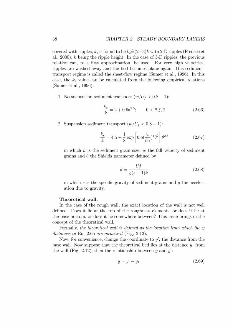
Figure 2.14: Turbulence quantities. Rough wall. Averaging over both time andspace. Sumer et al. (2001).
Fig. 2.14 shows data regarding u 2, v 2, and−u v . The data are plot-ted in a format slightly different from that in the above equation, namely,the actual roughness height is used to normalize y, rather than Nikurad-se’s equivalent sand roughness. Notice the large difference in the roughnessReynolds numbers of the two sets of data. Despite this, the good agreementbetween these two data may imply that the functions g1,.., g4 are universal.
Fig. 2.15 compares the turbulence quantities obtained in another study;in these tests, everything else is maintained unchanged, but the wall rough-ness is changed, to see the influence of the wall roughness on the end results.From the figure, the following two points are worth emphasizing:
1. The influence of the wall roughness disappears with the distance fromthe wall, as expected.
2. The distribution of turbulence across the depth is more uniform in thecase of the rough wall than in the case of the smooth wall.

2.2. FLOW ACROSS THE ENTIRE SECTION 43
Figure 2.15: Turbulence quantities. Grass (1971).
2.2 Flow across the entire section
In the preceding section, we have been concerned with the flow close to awall (a wall of an open channel, that of a pipe, etc.). In this section we willturn our attention to the flow across the entire section of the channel/pipe.Clearly, in this case, there will be an additional parameter, namely the flowdepth in the case of the channel-flow (or the pipe radius in the case of thepipe flow, or the boundary-layer thickness in the case of the boundary-layerflow).
Mean flow.In the analysis developed for flows close to a wall, the mean flow velocity
has been written as a function of four quantities, τ 0, y, μ, ρ (Eq. 2.9). Whenwe consider the flow across the entire section, however, two changes will takeplace:
1. There will be one additional parameter, namely the flow depth (orthe pipe radius, or the boundary-layer thickness) affecting the flow, asmentioned in the preceding paragraph (Fig. 2.2); and
44 CHAPTER 2. STEADY BOUNDARY LAYERS
2. The shear stress τ (Fig. 2.2),
τ = τ 0(1−y
h) (2.73)
will replace the wall shear stress τ 0 .
Hence, the velocity is now dependent of the following five parameters
u = F (τ , y, μ, ρ, h) (2.74)
However, from Eqs. 2.73 and 2.74, the preceding equation may be written as
u = F (τ 0, y, μ, ρ, h) (2.75)
From dimensional analysis, the following nondimensional function maybe obtained
u = Uf ϕ(Ufh
ν,y
h) (2.76)
Now, we will follow the same line of thought as in the preceding sections;namely, the variation of the velocity du
dyat large distances from the wall is
independent of the viscosity. Dropping out the viscosity in Eq. 2.75,
du
dy=d
dyF (τ 0, y, ρ, h)
or
Ψ1(du
dy, τ 0, y, ρ, h) = 0 (2.77)
and from dimensional analysis one obtains
du
dy=Ufh
ϕ1(y
h) (2.78)
Integrating gives
u = Uf ϕ1(y
h) d(
y
h) + c
and using the boundary condition
y = h : u = U0
one obtains
u− U0 = Ufy
y=h
ϕ1(y
h) d(
y
h)

2.2. FLOW ACROSS THE ENTIRE SECTION 45
Figure 2.16: Flow regions in a turbulent boundary layer.
or denoting the integral by another function, f1(yh),
u− U0 = Uf f1(y
h) (2.79)
in which U0 is the velocity at the free surface in the case of the open-channelflow, and the center line velocity in the case of the pipe flow. The precedingequation is known as the velocity-defect law. This velocity distribution issatisfied in the outer-flow region, Fig. 2.16.The explicit form of the function f1(
yh) can be found in the following way.
As sketched in Fig. 2.16, the outer region and the logarithmic layer isexpected to overlap over a certain y interval. Therefore, in the overlappingregion, the two velocity distributions, namely the logarithmic law (Eq. 2.42)and the velocity-defect law (Eq. 2.79), should be identical; therefore fromEqs. 2.42 and 2.79,
AUf ln(yUfν) + BUf ≡ U0 + Uf f1(
y
h) (2.80)
and solving the function f1
f1(y
h) = A ln(
y
h) +B (2.81)
Therefore, the velocity-defect law
u− U0 = Uf (A ln(y
h) +B ) (2.82)

46 CHAPTER 2. STEADY BOUNDARY LAYERS
Figure 2.17: Velocity distribution over the entire section of the pipe.
1. A is the same universal constant as in the analysis for the near-wallflow, i.e., A = 2.5.
2. B , on the other hand, is found from experiments as B = −0.8 for pipeflows (Monin and Yaglom, 1971). However, if Eq. 2.82 is assumed tobe applicable for the entire cross section, then B has to be B = 0.
3. Experiments show that the velocity-defect law begins to deviate fromthe measured velocity profiles (not very significantly, however) for y
h>
0.2− 0.3 (Fig. 2.17).
4. When the general form of the equation for the velocity is considered(Eq. 2.76), it will be seen that U0 is a function of the Reynolds number.From Eq. 2.80,
U0 = AUf ln(hUfν) + Uf(B −B ) (2.83)
5. The velocity-defect law is also given in terms of the cross-sectionalaverage velocity. In the case of the open-channel flow
V =1
h
h
y=0
u(y) dy
andV = U0 − Uf(A−B ) (2.84)
2.2. FLOW ACROSS THE ENTIRE SECTION 47
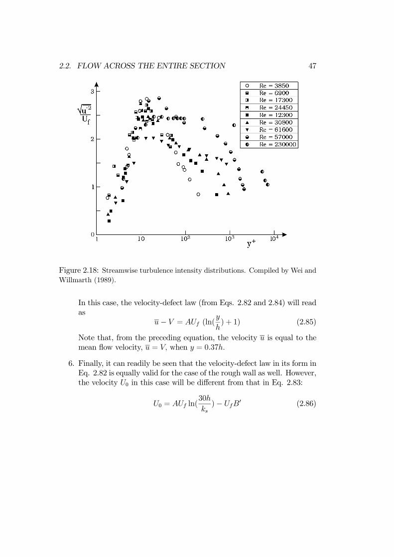
Figure 2.18: Streamwise turbulence intensity distributions. Compiled by Wei andWillmarth (1989).
In this case, the velocity-defect law (from Eqs. 2.82 and 2.84) will readas
u− V = AUf (ln(y
h) + 1) (2.85)
Note that, from the preceding equation, the velocity u is equal to themean flow velocity, u = V, when y = 0.37h.
6. Finally, it can readily be seen that the velocity-defect law in its form inEq. 2.82 is equally valid for the case of the rough wall as well. However,the velocity U0 in this case will be different from that in Eq. 2.83:
U0 = AUf ln(30h
ks)− UfB (2.86)

48 CHAPTER 2. STEADY BOUNDARY LAYERS
Figure 2.19: Transverse turbulence intensity distributions. Compiled by Wei andWillmarth (1989).
Turbulence quantities.The functional forms of the turbulence quantities depicted in Eq. 2.47
will include one additional parameter in the present case, namely hUfν, or
alternatively hVν, the Reynolds number.
Figs. 2.18 and 2.19 illustrates how this latter parameter influences theturbulence quantities u 2 and v 2 (Wei and Willmarth, 1989). As seen,near the wall, the effect of Re disappears, as expected (see Section 2.1.2).However, away from the wall, the Reynolds number significantly influences
the turbulence quantities. As Re increases,√u 2
Uf, and
√v 2
Ufincrease. This
is basically due to the increase in the flow depth when Re increases; indeed,the flow depth in terms of the wall parameters is like h+ ∼ Rep, p > 0 inwhich h+(= hUf
ν). (As Re increases, the turbulence generated near the wall
will be diffused to larger and larger h+, as revealed by Figs. 2.18 and 2.19).
2.3 Turbulence-modelling approach
The preceding sections give a considerable insight into the process of turbu-lent boundary layers in channels/pipes, and over walls. However, the methodused for the analysis does not enable us to do a parametric study, a study

2.3. TURBULENCE-MODELLING APPROACH 49
where the influence of various parameters on the boundary layer process canbe studied in a systematic manner. This can be achieved with the aid ofturbulence modelling. A detailed account of turbulence modelling is given inChapter 6. We restrict ourselves here only with the so-called mixing-lengthmodel and use it to address the problem of determining the mean velocitydistribution as function of the distance from the wall.
2.3.1 Turbulence modelling of flow close to a wall
Smooth wall.Our objective is to obtain the velocity distribution, u, near the wall (in
the constant-stress layer). The x− component of the Reynolds equation leadsto the following equation (Eq. 2.7):
τ(= μdu
dy+ (−ρu v )) = τ 0 (2.87)
in which there are two unknowns, namely u, and −ρu v . To close the system,we need a second equation. Drawing an analogy to Newton’s friction law
τ = μdu
dy(2.88)
the turbulence-induced shear stress can be written as
−ρu v = μtdu
dy(2.89)
in which μt is called turbulence viscosity. This is the simplest turbulencemodel, and was suggested by Boussinesq in 1877.The second step is to determine the turbulence viscosity in the above
equation. Making an analogy, this time, to the kinetic theory of gases, μt iswritten as
μt = ρ mVt (2.90)
in which m is what is called the mixing length (interpreted as the lengthof ”penetration” of fluid particles, or the length over which fluid parti-cles/parcels keep their coherence), and Vt is the turbulence velocity (a char-
acteristic velocity of the turbulent motion, for example, Vt ∼ v 2). Thehypothesis leading to Eq. 2.90 is known as Prandtl’s mixing-length hypoth-esis. The preceding equation is obtained in a different way in Chapter 6,Section 6.3.2.

50 CHAPTER 2. STEADY BOUNDARY LAYERS
There are two quantities to be ascribed in the preceding equation todetermine the turbulence viscosity: m and Vt. According to Prandtl’s secondhypothesis, these two quantities are related in the following way (see Chapter6, Section 6.3.2):
Vt = mdu
dy(2.91)
Clearly, it is expected that (1) the larger the mixing length, the larger the
turbulence velocity; and also (2) the larger the velocity gradient dudy, the
larger the turbulence generation (Section 1.4.3), and therefore the larger theturbulence velocity, revealing Eq. 2.91.From Eqs. 2.90 and 2.91, the turbulence viscosity
μt = ρ 2m
du
dy(2.92)
The third step is to determine the mixing length in the preceding equa-tion. van Driest (1956) gives the mixing length as follows
m = κy[1− exp(−y+
Ad)] (2.93)
in which κ is the von Karman constant (=0.4), and Ad is called the dampingcoefficient, and taken as 25. As seen,
m → κy, for large values of y+ (2.94)
while
m → 0, as y+ → 0 (2.95)
The latter implies that there will be no turbulence mixing as the wall isapproached.Eqs. 2.89, 2.92 and 2.93 are the model equations (three equations); so,
there are four equations altogether (along with the Reynolds equation, Eq.2.87), and four unknowns, namely, u, −ρu v , μt, and m (the latter alreadygiven by Eq. 2.93). Hence, the system is closed. Therefore the unknowns canbe determined. Let us focus on u.From Eqs. 2.87, 2.89 and 2.92, one gets
ρ 2m(du
dy)2 + μ
du
dy= τ 0 (2.96)

2.3. TURBULENCE-MODELLING APPROACH 51
Figure 2.20: Velocity distribution. Nezu and Rodi (1986).
Solving dudyfrom the preceding equation, and then substituting Eq. 2.93 into
the solution, and subsequently integrating gives
u = 2Ufy+
0
dy+
1 + 1 + 4κ2y+2[1− exp(−y+
Ad)]2
1/2(2.97)
The velocity distribution described by this expression is known as the vanDriest velocity profile, Fig. 2.20.
1. As seen from the figure, for small values of y+, the van Driest profilegoes to the linear velocity distribution in the viscous sublayer (Eq.2.35),
u
Uf= y+ (2.98)
while, for large values of y+, it goes to the logarithmic velocity distri-bution in the logarithmic layer (Eq. 2.42),
u = Uf (A ln y+ +B) (2.99)
2. Furthermore, the van Driest profile agrees remarkably well with themeasured velocity profile including the buffer layer (5 < y+ < 70).

52 CHAPTER 2. STEADY BOUNDARY LAYERS
Figure 2.21: van Driest velocity profiles for different values of roughness.
Regarding the other two unknowns, −ρu v and μt, inserting Eqs. 2.93and 2.97 in Eq.2.92, μt is obtained, and from this and Eqs. 2.97 and 2.89,−ρu v is obtained.Transitional and rough walls.In this case, the mixing length may be given as (Cebeci and Chang, 1978)
m = κ(y +∆y)[1− exp(−(y+ +∆y+)
Ad)] (2.100)
1. y in the above equation is the distance from the wall; it is measuredfrom the level where the velocity u is zero. This level lies almost at thetop of the roughness elements. (y here should not be confused with thedistance measured from the theoretical wall. As will be pointed outlater (Item 3 below), apparently y+∆y is the distance measured fromthe theoretical wall).
2. ∆y is the so-called coordinate displacement, or the coordinate shift (seeExample 5 below), and given by Cebeci and Chang (1978)
∆y+ = 0.9[ k+s − k+s exp(−k+s
6)]; 5 < k+s < 2000 (2.101)
2.3. TURBULENCE-MODELLING APPROACH 53
in which k+s is the roughness Reynolds number (ks being Nikuradse’sequivalent sand roughness):
k+s =ksUfν
(2.102)
3. Apparently, the distance y + ∆y is the distance measured from thetheoretical wall, as will be shown in Example 5.
Similar to the case of the smooth wall, u can be obtained from the modelequations, with m given in Eq. 2.100:
u = 2Ufy+
0
dy+
1 + 1 + 4κ2(y+ +∆y+)2[1− exp(− (y++∆y+)Ad
)]21/2
(2.103)
Fig. 2.21 displays the velocity profiles obtained from Eq. 2.103 including thesmooth-wall profile. In Fig. 2.21, a represents the linear profile in the viscoussublayer (Eq. 2.98), b the logarithmic profile in the case of the hydraulicallysmooth wall (Eq. 2.99), and c the logarithmic profile in the case of thecompletely rough wall (Eq. 2.65), namely, by putting z = y +∆y,
u = AUf ln(30z
ks) (2.104)
z being measured from the theoretical wall.
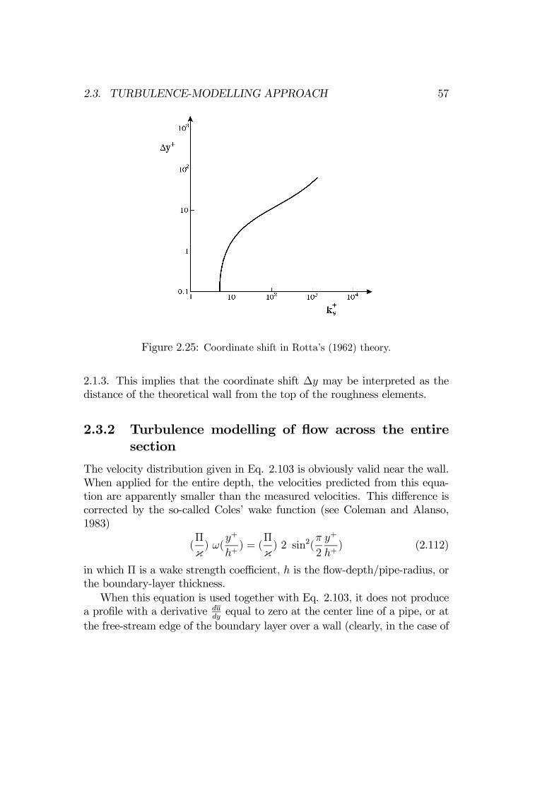
Example 5 Rotta’s (1962) theory about the coordinate shift ∆y.
The velocity distribution for large y+ values is written in the followingform:
u = Uf [1
κln y+ + c(k+s )] (2.105)
in which y is measured from the level where the velocity u = 0 (not to beconfused with y measured from the theoretical wall). The function c(k+s ) inthe above equation is determined from Nikuradse’s experiments (Fig. 2.22).Note that 1 < k+s < 1000 (see the figure).For the smooth-wall case, the preceding equation reduces to
u = Uf [1
κln y+ + c(0)] (2.106)
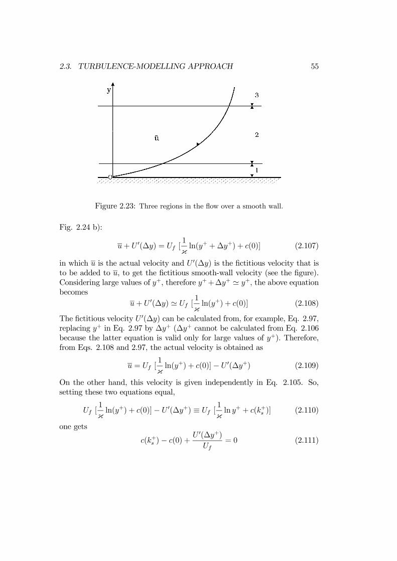
Now, in the case of the smooth wall, we know that there are three distinctregions, namely,

54 CHAPTER 2. STEADY BOUNDARY LAYERS
Figure 2.22: Function c(k+s ) in Rotta’s (1962) theory.
1. y+ < 5 where the momentum transfer across the depth is due to vis-cosity (Region 1, Fig. 2.23);
2. 5 < y+ < 70 where this transfer is due to both viscosity and turbulence(Region 2, Fig. 2.23); and
3. y+ > 70 where it is practically due to turbulence alone (Region 3, Fig.2.23).
In the case of the transitional/rough wall, Region 2 and Region 3 are stillpresent (Fig. 2.24 a). However, Region 1 is practically not existent. Now, weimagine a fictitious region (Region 1) just beneath Region 2, where a fictitiousmomentum transfer takes place. Let us assume that this momentum transferis due to viscosity. Let the thickness of this layer be∆y. So, with the additionof this fictitious layer, the flow over the rough wall will be ”identical” to thatover the smooth wall. Therefore, we can implement the smooth-wall velocitydistribution (Eq. 2.106) for the present case (with the wall coordinate y+∆y,
2.3. TURBULENCE-MODELLING APPROACH 55
Figure 2.23: Three regions in the flow over a smooth wall.
Fig. 2.24 b):
u+ U (∆y) = Uf [1
κln(y+ +∆y+) + c(0)] (2.107)
in which u is the actual velocity and U (∆y) is the fictitious velocity that isto be added to u, to get the fictitious smooth-wall velocity (see the figure).Considering large values of y+, therefore y++∆y+ y+, the above equationbecomes
u+ U (∆y) Uf [1
κln(y+) + c(0)] (2.108)
The fictitious velocity U (∆y) can be calculated from, for example, Eq. 2.97,replacing y+ in Eq. 2.97 by ∆y+ (∆y+ cannot be calculated from Eq. 2.106because the latter equation is valid only for large values of y+). Therefore,from Eqs. 2.108 and 2.97, the actual velocity is obtained as
u = Uf [1
κln(y+) + c(0)]− U (∆y+) (2.109)
On the other hand, this velocity is given independently in Eq. 2.105. So,setting these two equations equal,
Uf [1
κln(y+) + c(0)]− U (∆y+) ≡ Uf [
1
κln y+ + c(k+s )] (2.110)
one gets
c(k+s )− c(0) +U (∆y+)
Uf= 0 (2.111)

56 CHAPTER 2. STEADY BOUNDARY LAYERS
Figure 2.24: Flow over a rough wall in Rotta’s (1962) theory.
Given the function c(k+s ) (Fig. 2.22), and U (∆y+) from Eq. 2.97,
U (∆y+) = 2Uf∆y+
0
dy+
1 + 1 + 4κ2∆y+2[1− exp(−∆y+
Ad)]2
1/2
the coordinate shift ∆y+ can be calculated from Eq. 2.111. Rotta (1962)carried out this calculation. Fig. 2.25 shows the result.It may be noted that the variation depicted in Fig. 2.25 agrees fairly well
with the expression given by Cebeci and Chang (1978) in Eq. 2.101.As a final remark, the coordinate shift normalized by the roughness
height,∆yk, can be found from Eq. 2.101 (where ks may be taken as 2k).
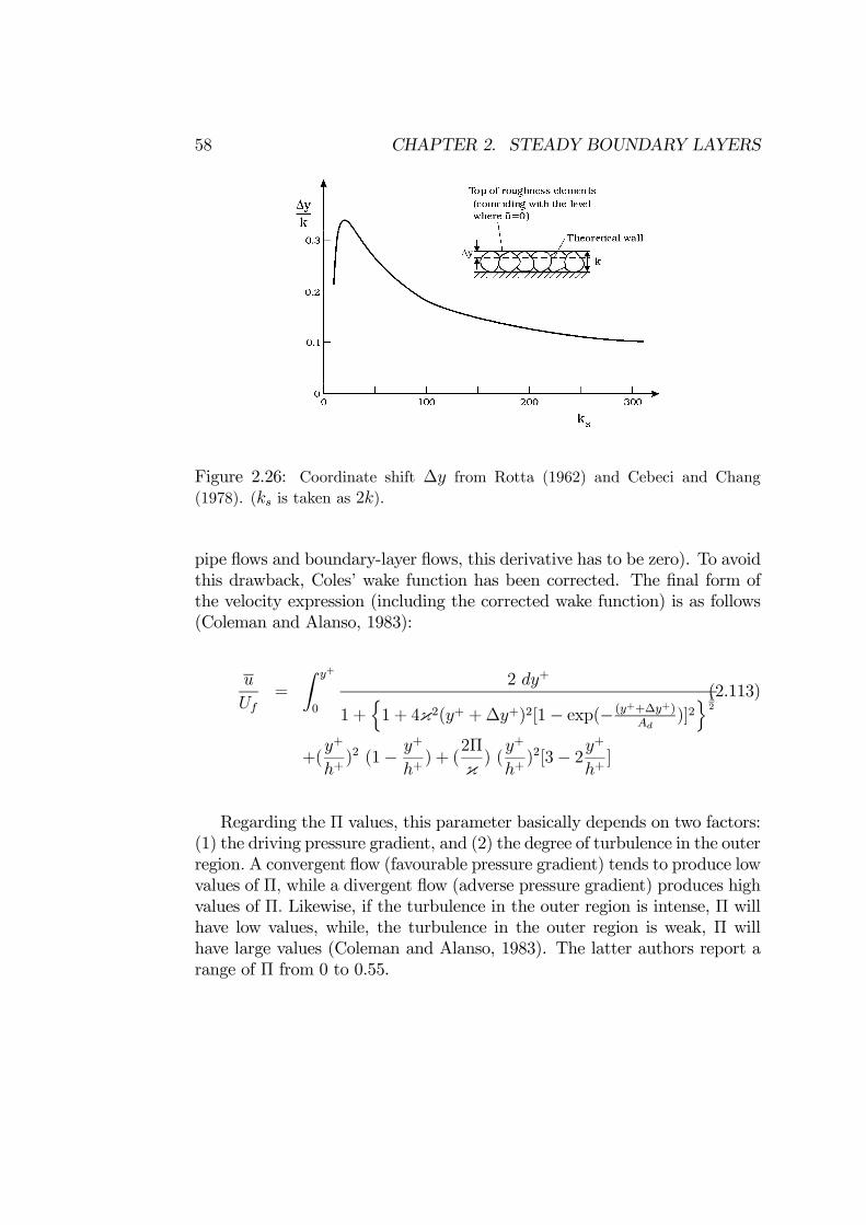
The result of this exercise is plotted in Fig. 2.26. As seen, the ∆ykvalues
exhibited in the figure agree rather well with the experimental observationsthat the level of the theoretical bed lies (0.15-0.35)k below the top of theroughness elements, given in conjunction with the theoretical bed in Section
2.3. TURBULENCE-MODELLING APPROACH 57
Figure 2.25: Coordinate shift in Rotta’s (1962) theory.
2.1.3. This implies that the coordinate shift ∆y may be interpreted as thedistance of the theoretical wall from the top of the roughness elements.
2.3.2 Turbulence modelling of flow across the entiresection
The velocity distribution given in Eq. 2.103 is obviously valid near the wall.When applied for the entire depth, the velocities predicted from this equa-tion are apparently smaller than the measured velocities. This difference iscorrected by the so-called Coles’ wake function (see Coleman and Alanso,1983)
(Π
κ) ω(
y+
h+) = (
Π
κ) 2 sin2(
π
2
y+
h+) (2.112)
in which Π is a wake strength coefficient, h is the flow-depth/pipe-radius, orthe boundary-layer thickness.When this equation is used together with Eq. 2.103, it does not produce
a profile with a derivative dudyequal to zero at the center line of a pipe, or at
the free-stream edge of the boundary layer over a wall (clearly, in the case of
58 CHAPTER 2. STEADY BOUNDARY LAYERS
Figure 2.26: Coordinate shift ∆y from Rotta (1962) and Cebeci and Chang(1978). (ks is taken as 2k).
pipe flows and boundary-layer flows, this derivative has to be zero). To avoidthis drawback, Coles’ wake function has been corrected. The final form ofthe velocity expression (including the corrected wake function) is as follows(Coleman and Alanso, 1983):
u
Uf=
y+
0
2 dy+
1 + 1 + 4κ2(y+ +∆y+)2[1− exp(− (y++∆y+)Ad
)]212
(2.113)
+(y+
h+)2 (1− y
+
h+) + (
2Π
κ) (y+
h+)2[3− 2y
+
h+]
Regarding the Π values, this parameter basically depends on two factors:(1) the driving pressure gradient, and (2) the degree of turbulence in the outerregion. A convergent flow (favourable pressure gradient) tends to produce lowvalues of Π, while a divergent flow (adverse pressure gradient) produces highvalues of Π. Likewise, if the turbulence in the outer region is intense, Π willhave low values, while, the turbulence in the outer region is weak, Π willhave large values (Coleman and Alanso, 1983). The latter authors report arange of Π from 0 to 0.55.

2.4. FLOW RESISTANCE 59
2.4 Flow resistance
The question here is that, given the mean flow velocity V, how we can cal-culate the friction velocity Uf , i.e.,
Uf =τ 0ρ
(2.114)
This issue may be best described by reference to a circular pipe flow.For a smooth circular pipe, the flow velocity is given by Eq. 2.42 with
coefficients given in Eq. 2.43. Schlichting (1979, p. 603) takes it in thefollowing, slightly different form:
u = Uf (2.5 ln y+ + 5.5) (2.115)
Assuming that this velocity distribution is, to a first approximation, validacross the entire section, and therefore putting y = R, the pipe radius, willgive:
U0 = Uf (2.5 ln(RUfν) + 5.5) (2.116)
On the other hand, we have obtained in the preceding paragraphs a relation-ship between the mean flow velocity and the maximum velocity (Eq. 2.84),which reads
V = U0 − (A−B )Uf (2.117)
Now, Schlichting (1979, p.609) takes this relation in the following form
V = U0 − 3.75Uf (2.118)
Combining Eq. 2.116 with Eq. 2.118, we obtain the following equation(Schlichting, 1979, p. 610)
1√8
V
Uf= 2.035 log(
V D
ν
√8UfV)− 0.91 (2.119)
in which D is the pipe diameter. (Note that log in the above equation shouldnot be confused with the natural logarithm). The coefficients can be adjustedslightly so that the preceding equation agrees with the experimental data.This latter exercise gives the following relation
1√8
V
Uf= 2.0 log(
V D
ν
√8UfV)− 0.8 (2.120)
60 CHAPTER 2. STEADY BOUNDARY LAYERS
This is Prandtl’s universal law of friction for smooth pipes (Schlichting, 1979,p.611).In the case of a rough circular pipe, we can do the same exercise, but this
time with the velocity distribution given by Eq. 2.65
u = AUf ln(30y
ks) (2.121)
Putting y = R in the above equation
U0 = AUf ln(30R
ks) (2.122)
and combining Eqs. 2.122 and 2.118, we get (Schlichting, 1979, p. 621)
UfV=
1√8(2 log R
ks+ 1.68)
(2.123)
A comparison with Nikuradse’s experimental results shows that closer agree-ment can be obtained, if the constant 1.68 is replaced by 1.74 (Schlichting,1979, p.621):
UfV=
1√8(2 log R
ks+ 1.74)
(2.124)
In the case of a transitional-wall-category circular pipe, Colebrook andWhite obtains the following resistance relation (Schlichting, 1979, p.621)
1√8
V
Uf= 1.74− 2 log(ks
R+
18.7
(V Dν)(√8UfV)) (2.125)
Given the mean-flow velocity, the friction velocity can easily be calculatedfrom Eqs. 2.120, 2.124 or 2.125.In the case of a non-circular pipe flow or an open flow, the preceding
resistance relations can be used provided that the pipe diameter D shouldbe replaced by 4rh in which rh is the hydraulic radius, equal to the cross-sectional area divided by the wetted perimeter (Schlichting, 1979, p. 622).For example, in the case of an open channel with a rough bed, the resistancerelation can be found as
V
Uf= 5.75 log(
14.8rhks
) (2.126)

2.5. BURSTING PROCESS 61
orV
Uf= 2.5 ln(
14.8rhks
) (2.127)
It may be noted that the ratio V/Uf may be traditionally written in termsof the friction coefficient, f, as
Uf =f
2V (2.128)
Figure 2.27: Snapshot of flow near the wall.
2.5 Bursting process
Experimental work conducted in 1960s and 70s has shown that the natureof the flow pattern near the wall in a turbulent boundary layer is repetitive;the flow near the wall occurs in the form of a quasi-cyclic process, called thebursting process. Reviews of the subject can be found in Laufer (1975), Hinze(1975, pp. 659-668), Cantwell (1981), Grass (1983) and Nezu and Nakagawa(1993).

62 CHAPTER 2. STEADY BOUNDARY LAYERS
Figure 2.28: Flow separation induced by adverse pressure gradient.
The description of the bursting process in the following paragraphs ismainly based on the work of Offen and Kline (1973, 1975).Fig. 2.27 gives a snapshot of the flow picture near the wall. As seen, the
flow consists of a transverse alternation of low-speed (A) and high-speed (B)regions. These are called low-speed and high-speed streaks. The low-speedand high-speed streaks form locally and temporarily.Similar to the separation of a boundary layer subject to an adverse pres-
sure gradient (such as, for example, the boundary layer separation over acylinder, see Fig. 2.28 a), a low-speed wall streak is subject to separationdue to a local and temporary adverse pressure gradient ∂p
∂x, Fig. 2.28 b. This
causes this coherent, low-speed fluid to entrain into the main body of theflow. This is called the ejection event. See Fig. 2.29, Frames 1 and 2.The fluid ejected into the flow grows in size, as it is convected downstream,
while keeping its coherent entity. This continues for some period of time (Fig.2.29, Frame 3), and finally, at some point (t = T ), the previously mentionedcoherent structure breaks up (Fig. 2.29, Frame 4). At this point, some fluidfrom the coherent structure returns back to the near-wall region (Fig. 2.29,Frame 5). This fluid impinges the wall (in the form of a high-speed wallstreak, called the in-rush event), and spreads out sideways (Fig. 2.29, Frame6). Two-such neighbouring high-speed streaks eventually merge (Fig. 2.29,Frame 6), and retard the flow there, and, as a result, a new low-speed wallstreak is formed. The time period spent from the formation of the low-speedstreak at time t = 0 (Fig. 2.29, Frame 1) to the formation of the next oneat time t = T1 (Fig. 2.29, Frame 6) is called the bursting period. After theformation of this new low-speed streak, the same chain of events occurs, andthe process continues in a repetitive manner.Fig. 2.30 displays two snapshots (viewed from the side), illustrating the

2.5. BURSTING PROCESS 63
Figure 2.29: Sequence of flow pictures over one bursting period.

64 CHAPTER 2. STEADY BOUNDARY LAYERS
Figure 2.30: (a): ejection; and (b): in-rush events. Grass (1971).
ejection event (Fig. 2.30, a), and the in-rush event (Fig. 2.30 b).The bursting process has been studied in the case of rough walls, and it
was found that practically the same kind of quasi-cyclic process takes place(Grass, 1971, and Grass et al., 1991).The rest of this section is concerned with quantitative information on the
bursting process.
1. The mean spacing of the low-speed wall streaks (Fig. 2.29, Frame 1) is
λ+ =λUfν
100 (2.129)
(see for example, Lee et al., 1974)
2. Fluid ejections originate in
5 < y+ < 50 (2.130)
(Nychas et al., 1973). Corino and Brodkey (1969), on the other hand,report that lower half of the viscous sublayer y+ < 2.5 is essentially
2.5. BURSTING PROCESS 65
passive and the rest (2.5 < y+ < 5) active, being influenced by thequasi-cyclic, bursting events occurring in 5 < y+ < 70.
3. The x− and z−extents of ejected low-speed fluid structures involvedimensions of the order of
20 to 40 of x+, and 15 to 20 of z+ (2.131)
4. Ejected fluid elements reach y+s of
y+ = 80− 100 (2.132)
(Nychas et al., 1973). Praturi and Brodkey (1978) report that, in somerare cases, the ejected fluid elements travel up to 300 y+).
5. The mean streamwise distance from the onset of lift-up of a low-speedwall streak to the break-up of any sign of coherency is about
1300 in x+ (2.133)
(Offen and Kline, 1973).
6. The mean time between the onset of ejection and break-up (the lifetime of a burst) is
TU0h
= 2.3 for the smooth boundary data, and (2.134)
1.3 for the rough boundary data
of the study by Jackson (1976). As seen, T scales with the outer flowparameters, namely U0, the free-stream velocity (or the velocity at thefree surface in the case of the open channel flow), and h is the boundary-layer thickness/the flow depth.
7. Finally, the mean bursting period
T1U0h
= 5 (2.135)
(Jackson, 1976). Note that this, too, scales with the outer flow para-meters.

66 CHAPTER 2. STEADY BOUNDARY LAYERS
There have been several implications of this newly discovered aspect ofturbulent boundary-layer flows. One of them is the process of sedimentsuspension in rivers and in the marine environment. The work conducted in1970s and 80s indicated that the bursting process is the key mechanism forsediment suspension from/near the bed (see, for example, Sumer and Oguz,1978, Sumer and Deigaard, 1981, Grass, 1983, and Sumer, 1986).
2.6 Appendix. Dimensional analysis
We may write the unit of any hydrodynamic quantity in the following form
[A] = LαT βKγ (2.136)
in which [A] is the unit of A, and L, T, and K are the fundamental units,namely, L is the length, T the time, and K is the force. α,β and γ arepositive or negative integers, or they may be zero.Now, Buckingham’s Pi Theorem states the following.A dimensional function
f(A1, A2, ...., An) = 0 (2.137)
can always be converted to the following nondimensional function
F (π1,π2, ......πn−r) = 0 (2.138)
in which Ai (i = 1, .....n) are the dimensional quantities, and r is the numberof the fundamental units (normally r = 3, i.e., the length, the time and theforce). The quantities πi (i = 1, ..., n− r) are the nondimensional quantitiesand calculated from
π1 = Ax11 Ay12 A
z13 A4 (2.139)
π1 = Ax21 Ay22 A
z23 A4
..........
πn−r = Axn−r1 Ayn−r2 Azn−r3 A4
Note that the above combinations of Ai (for each πi) should be selected sothat
1. The unit of any one of Ai should not be a combination of the units ofthe others; and

2.6. APPENDIX. DIMENSIONAL ANALYSIS 67
2. Each and every fundamental unit should be included in at least one ofthe Ai’s.
The advantage of the dimensional analysis is that, first of all, it ”trans-lates” the dimensional function into a nondimensional function in a system-atic way, secondly and more importantly, in doing so, the number of thequantities included in the dimensional function is reduced by r (normallyr = 3).
Example 6 Law of the wall.
In Section 2.1.1, the flow velocity is written as a function of the followingnondimensional quantities (Eq. 2.9)
u = F (τ 0, y, μ, ρ) (2.140)
orf(τ 0, μ, ρ, u, y) = 0 (2.141)
As seen, n = 5, and therefore the number of nondimensional quantities willbe n− r = 5− 3 = 2. Hence
F (π1,π2) = 0 (2.142)
in which the nondimensional quantities π1 and π2
π1 = τx10 μy1 ρz1 u (2.143)
andπ2 = τx20 μy2 ρz2y (2.144)
The left and right hand sides of Eq. 2.143 should have the same units.Writing the units of the quantities on both sides of the equation accordingto Eq. 2.136,
L0T 0K0 = (KL−2)x1(KL−2T )y1(KL−4T 2)z1(LT−1) (2.145)
orL0T 0K0 = L−2x1−2y1−4z1+1T y1+2z1−1Kx1+y1+z1 (2.146)

68 CHAPTER 2. STEADY BOUNDARY LAYERS
which requires
−2x1 − 2y1 − 4z1 + 1 = 0, (2.147)
y1 + 2z1 − 1 = 0,
x1 + y1 + z1 = 0
This gives
x1 = −1
2, y1 = 0, and z1 =
1
2(2.148)
Hence the first nondimensional quantity
π1 = τ−1/20 μ0ρ1/2u =
u
( τ0ρ)1/2
=u
Uf(2.149)
Regarding the second nondimensional quantity, from Eq. 2.144
L0T 0K0 = (KL−2)x2(KL−2T )y2(KL−4T 2)z2L (2.150)
and
−2x2 − 2y2 − 4z2 + 1 = 0, (2.151)
y2 + 2z2 = 0,
x2 + y2 + z2 = 0
andx2 =
1
2, y2 = −1, and z2 =
1
2(2.152)
Then, the second nondimensional quantity
π2 = τ1/20 μ−1ρ1/2y =
y( τ0ρ)1/2
μρ
=yUfν
(2.153)
Therefore, the nondimensional function will be
F (u
Uf,yUfν) = 0 (2.154)
or solving the velocityu
Uf= f(
yUfν) (2.155)
This relation is known as the law of the wall.

2.7. REFERENCES 69
2.7 References
1. Bayazit, M. (1976): ”Free surface flow in a channel of large relativeroughness”, J. Hyd. Res., 14, no. 2, 1976, p. 115.
2. Bayazit, M. (1983): ”Flow structure and sediment transport mechanicsin steep channels. In: Mechanics of Sediment Transport, Proc. ofEuromech 156, Istanbul, 12-14. July 1982, A.A. Balkema (Rotterdam),p.197.
3. Cantwell, B.J. (1981): ”Organized motion in turbulent flow”. Ann.Rev. Fluid Mech., vol 13, p.457.
4. Cebeci, T. and Chang, K.C. (1978): ”Calculation of incompressiblerough-wall boundary-layer flows”. AIAA Journal, vol. 16, No. 7,p.730.
5. Coleman, N.L. and Alanso, C.V. (1983): ”Two-Dimensional channelflows over rough surfaces”. J. Hydraul. Eng., Proc. ASCE, vol 109,No. 2, p.175.
6. Corino, E.R. and Brodkey, R.S. (1969): ”A visual investigation of thewall region in turbulent flow”. J. Fluid Mech., vol. 37, p.1.
7. Engelund, F. and Hansen, E. (1967): AMonograph on Sediment Trans-port in Alluvial Streams, Teknisk Forlag, Copenhagen.
8. Fredsøe, J. Andersen, K.H. and Sumer, B.M. (2000): ”Wave plus cur-rent over a ripple-covered bed”. Coastal Engineering.
9. Grass, A.J. (1971): ”Structural features of turbulent flow over smoothand rough boundaries”. J. Fluid Mech., vol. 50, p.233.
10. Grass, A.J. (1983): ”The influence of boundary layer turbulence on themechanics of sediment transport”. In: Mechanics of Sediment Trans-port, Proc. of Euromech 156, Istanbul, 12-14. July 1982, A.A. Balkema(Rotterdam).
11. Grass, A.J., Stuart, R.J. and Mansour-Tehrani, M. (1991): ”Vorti-cal structures and coherent motion in turbulent flow over smooth andrough boundaries”, Phil. Trans. R. Soc. London A, vol. 336, p. 35.

70 CHAPTER 2. STEADY BOUNDARY LAYERS
12. Hinze, J.O. (1975): Turbulence. McGraw-Hill.
13. Jackson, R.G. (1976): ”Sedimentological and fluid-dynamic implica-tions of the turbulent bursting phenomenon in geopyhsical flows”. J.Fluid Mech., vol. 77, p. 531.
14. Kamphuis, J. W. (1974): ”Determination of sand roughness for fixedbeds”. J. Hydraulic Res., Vol. 12, No.2, p.193.
15. Laufer, J. (1954): The Structure of Turbulence in Fully Developed PipeFlow. NACA, Report No. 1174.
16. Laufer, J. (1975): ”New trends in experimental turbulence research”.Ann. Review of Fluid Mech., vol. 7, p.307.
17. Lee, M.K., Eckelman, L.D., Hanratty, T.J. (1974): ”Identification ofturbulent wall eddies through the phase relation of the components ofthe fluctuating velocity gradient”. J. Fluid Mech., vol. 66, p. 17.
18. Monin, A. S. and Yaglom, A. M. (1973): Statistical Fluid Mechanics:Mechanics of Turbulence. MIT Press, Cambridge, Mass.
19. Nezu, I. and Rodi, W. (1986): ”Open-Channel flow measurements witha laser Doppler anemometry”. ASCE J. Hyd. Eng., vol. 112, No. 5,335-355.
20. Nezu, I. and Nakagawa, H. (1993): Turbulence in Open-Channel Flow.IAHR Monograph, A.A. Balkema (Roterdam).
21. Nychas, S.G., Hershey, H.C. and Brodkey, R.S. (1973): ”A visual studyof turbulent shear flow”. J. Fluid Mech., vol. 61, p. 513.
22. Offen, G.R. and Kline, S.J. (1973): Experiments on the velocity char-acteristics of ”Bursts” and on the Interactions Between the Inner andOuter Regions of a Turbulent Boundary Layer. Dept. of Mech. Engrg.,Stanford University, Report MD-31.
23. Offen, G.R. and Kline, S.J. (1975): ”A proposed model of the burstingprocess in turbulent boundary layers”. J. Fluid Mech.., vol. 70, p. 209.

2.7. REFERENCES 71
24. Praturi, A.K. and Brodkey, R.S. (1978): ”A stereoscopic visual studyof coherent structures in turbulent shear flow. J. Fluid Mech., vol. 89,p.251.
25. Rotta, J.C. (1962). ”Turbulent boundary layers in incompressible flow”.Progress in Aerospace Science, vol. 2, p.1.
26. Schlichting, H. (1979). Boundary-Layer Theory. McGraw-Hill.
27. Sumer, B.M. (1986): ”Recent Developments on the Mechanics of sedi-ment suspension”, General-Lecture Paper, in the book: Euromech 192:Transport of suspended solids in open channels, A.A. Balkema Pub-lishers, Rotterdam, 1986.
28. Sumer, B.M., Cokgor, S. and Fredsøe, J. (2001): ”Suction removal ofsediment from between armour blocks”. Journal of Hydraulic Engi-neering, ASCE, vol. 127, No. 4, pp. 293-306, 2001.
29. Sumer, B.M. and Deigaard, R. (1981): ”Particle motions near the bot-tom in turbulent flow in an open channel - Part 2”. Journal of FluidMechanics, Vol. 109, p. 311.
30. Sumer, B.M. and Oguz, B. (1978): ”Particle motions near the bottomin turbulent flow in an open channel”. Journal of Fluid Mechanics, Vol.86, p. 109, 1978.
31. Sumer, B.M., Kozakiewicz, A., Fredsøe, J. and Deigaard, R. (1996):”Velocity and concentration profiles in the sheet flow layer of movablebed”. Journal of Hydraulic Engineering, ASCE, vol. 122, No. 10,549-558.
32. van Driest, E.R. (1956): ”On turbulent flow near a wall”. J. Aeronau-tical Sciences, vol. 23, p.1007.
33. Wei, T. and Willmarth, W.W. (1989): ”Reynolds-number effects onthe structure of a turbulent channel flow”. J. Fluid Mech., vol. 204, p.57.

72 CHAPTER 2. STEADY BOUNDARY LAYERS
Chapter 3
Statistical analysis
As has been seen in the previous chapters, hydrodynamic quantities suchas the velocity components appear to be random variables. Although re-cent research has shown that the near-wall turbulent-boundary-layer processis repetitive in nature (Chapter 3, Bursting Process), unless special pat-tern recognition techniques are used to detect these repetitive, quasi-cyclicevents, the turbulence signals even near the wall appear to be largely ran-dom. Therefore, it is imperative to use statistical techniques to study theturbulence.Three topics will be discussed in the present chapter. First we will briefly
study the probability density function of the turbulent velocity, then we willconcentrate on the correlation and subsequently spectral analysis of turbu-lence. In the entire analysis, it will be assumed that the turbulence is isotropicunless otherwise stated.
3.1 Probability density function
Consider, for example, the x− component of the velocity, u (Fig. 3.1 a). Thevelocity u (or its fluctuating component u ) is a random variable. Thus, u(or u ) must have a probability density function (p.d.f.) such that
p(u ) du = Pr[u < U < u + du ] (3.1)
and ∞
−∞p(u ) du = 1 (3.2)
73

74 CHAPTER 3. STATISTICAL ANALYSIS
Figure 3.1: Time series and p.d.f. of velocity.
in which p(u ) is the p.d.f. of the fluctuating velocity u , and Pr[u < U <u + du ] is the probability of occurrence of the fluctuating velocity betweenu and u + du .Experiments show that p(u ) can be represented by the Gaussian (normal)
distribution
p(u ) =1
σu√2πexp(− u
2
2σ2u) (3.3)
in which σu is the standard deviation of the velocity of u :
σu = (u− u)2 = u 2 (3.4)
The significance of σu is that the probability of occurrence of u outside therange, for example, −2σu < u < +2σu is only 4.6%, while that outside therange −3σu < u < +3σu is even much smaller, namely 0.3% (if the p.d.f. isrepresented by the Gaussian distribution).It may be noted that the p.d.f. of the fluctuating velocity components
may be different from the Gaussian distribution, with non-zero skewness,particularly near the wall (see the measurements made very close to the wall,reported in Eckelmann, 1974). This may be linked to the bursting process(Chapter 3).Fig. 3.2 shows the p.d.f.’s (in the form of frequency histograms) for the
two components of the turbulent velocities, u and v, near the wall for threedifferent boundaries, namely the smooth, transitional and rough walls. Notethe non-zero skewness in all distributions.The statistical moments (or central moments) also give some information
on the statistical properties of the velocities and other quantities:
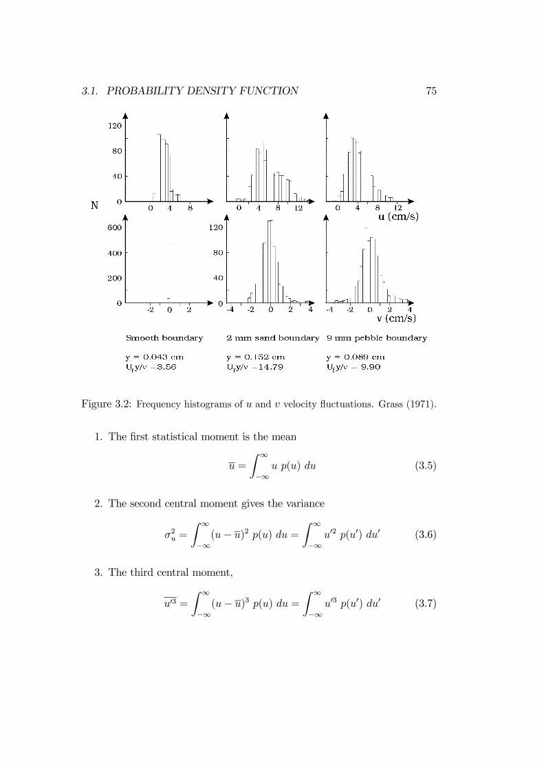
3.1. PROBABILITY DENSITY FUNCTION 75
Figure 3.2: Frequency histograms of u and v velocity fluctuations. Grass (1971).
1. The first statistical moment is the mean
u =∞
−∞u p(u) du (3.5)
2. The second central moment gives the variance
σ2u =∞
−∞(u− u)2 p(u) du =
∞
−∞u 2 p(u ) du (3.6)
3. The third central moment,
u 3 =∞
−∞(u− u)3 p(u) du =
∞
−∞u 3 p(u ) du (3.7)

76 CHAPTER 3. STATISTICAL ANALYSIS
gives the skewness factor :
Su =u 3
(σ2u)32
(3.8)
4. The fourth central moment,
u 4 =∞
−∞(u− u)4 p(u) du =
∞
−∞u 4 p(u ) du (3.9)
gives the flatness factor:
Fu =u 4
(σ2u)2
3.2 Correlation analysis
There are two kinds of correlations: (1) Space correlations, and (2) timecorrelations. We will first focus on the space correlations.
3.2.1 Space correlations
Definitions.Fig. 3.3 gives the definition sketch. Consider the i− component of the
fluctuating velocity at Point A, (ui)A, and j− component of the fluctuat-ing velocity at Point B, (uj)B. Suppose that these velocities are measuredsimultaneously.Two-point double correlation is defined by
(Oij)AB = (ui)A (uj)B (3.10)
in which the overbar indicates the time averaging (Eq. 1.1). There areother correlations as well: three-point, four-point,..., and triple, quadru-ple,...correlations.Two most important two-point double correlations (Fig. 3.4) are
u (x) u (x+ r) (3.11)
andv (x) v (x+ r) (3.12)

3.2. CORRELATION ANALYSIS 77
Figure 3.3: Correlation measurement.
in which r is the separation between the two points.For convenience, these correlations are normalized by u 2 and v 2, respec-
tively:
f(r) =u (x) u (x+ r)
u 2(3.13)
g(r) =v (x) v (x+ r)
v 2(3.14)
f(r) and g(r) are called the correlation coefficients.The physical interpretation of the correlation functions/coefficients is as
follows. The larger the correlation, the better correlated the motions at thetwo measurement points, and therefore the more likely that these two pointsbelong to the same coherent structure. This would obviously give an ideaabout the length scale of the coherent structures, as will be detailed later inthe section.
Properties of two-point double correlations.
1. The correlation coefficients are unity at r = 0:
f(0) = g(0) = 1 (3.15)

78 CHAPTER 3. STATISTICAL ANALYSIS
Figure 3.4: Correlation measurement.
(from Eqs. 3.13 and 3.14).
2. There is symmetry between positive and negative separations:
f(r) = f(−r), and g(r) = g(−r) (3.16)
(from the requirement of homogeneity).
3. The correlation coefficients are smaller than or equal to unity:
f(r) ≤ 1, and g(r) ≤ 1 (3.17)
This can easily be seen from
(u (x)− u (x+ r))2 = u 2(x) + u 2(x+ r)− 2u (x)u (x+ r)= 2(u 2 − u (x)u (x+ r))
Since the left hand side of the equation ≥ 0, then u 2−u (x)u (x+ r) ≥0, hence f(r) ≤ 1.
4. The correlation coefficients tend to zero as the separation distance goesto infinity
f(r)→ 0, and g(r)→ 0, as r →∞ (3.18)
This is because when r is very large, there will be as many u (x)u (x+r)products with the negative sign as with the positive sign, therefore,when averaged, u (x)u (x+ r) will be zero. Physically, r is so largethat the two points will not lie in the same coherent structure, there-fore, their motions will be uncorrelated, meaning that the correlationcoefficients should be zero for such large r distances.

3.2. CORRELATION ANALYSIS 79
Figure 3.5: Correlation coefficients f and g, and micro scales.
5. While f(r) is always positive, g(r) can take negative values as well. Toshow this, we employ
rg(r) = rf(r) +1
2r2∂f
∂r=1
2
∂
∂r(r2f(r)) (3.19)
This is the relationship between f(r) and g(r) in isotropic turbulence,as will be detailed in the following paragraphs. Integrating gives
∞
0
rg(r)dr =1
2[r2f(r)]∞0 = 0 (3.20)
provided that r2f(r) = 0 as r → ∞. (Experiments show that f(r) islike f(r) ∼ e−r, then it is easy to see that r2f(r)→ 0 as r →∞.) Forthe integral on the left hand side of the equation to be zero, clearlyg(r) must have positive and negative values.
The general forms of the functions of f(r) and g(r) are shown in Fig. 3.5.Finally, we note the following. There is a special class of turbulence,
called isotropic turbulence where turbulence characteristics such as u 2 areindependent of the rotation of the axes. This implies that u 2 = v 2 = w 2.Turbulence in the ”core” region in a wind tunnel (where the wall effectsare practically nonexistent) may be considered to be isotropic. In such aturbulence field, the correlations coefficients are related with the followingequation
g(r) = f(r) +r
2
∂
∂rf(r) (3.21)
(see Hinze, 1959, p. 150).

80 CHAPTER 3. STATISTICAL ANALYSIS
Scales of turbulence.Micro scales. Expanding f(r) as a Taylor series, and for small values
of r, gives
f(r) = 1 +1
2(∂2f
∂r2)r=0 r2 + ... (3.22)
Note that the terms with rn (n being an odd number, n = 1, 3, 5, ..) will dropbecause f(r) = f(−r).Now, the formal definition of the micro time scale is
1
λ2f= −1
2(∂2f
∂r2)r=0 (3.23)
in which λf is the micro length scale of turbulence. Inserting the precedingequation in Eq. 3.22, one gets
f(r) = 1− r2
λ2f(3.24)
As seen from Fig. 3.5, this is a parabola fit to the correlation coefficient forsmall values of r , and λf is the x− intercept of the fitted parabola.Likewise,
g(r) = 1− r2
λ2g(3.25)
in which λg is another micro length scale.These length scales can also be expressed in terms of the fluctuating-
velocity gradients:1
λ2f=
1
2u 2(∂u
∂r)2 (3.26)
and1
λ2g=
1
2v 2(∂v
∂r)2 (3.27)
(see Raudkivi and Callander, 1975, p. 167).λf and λg are not independent of each other. In isotropic turbulence,
from Eq. 3.21,
(∂2
∂r2g(r))r=0 = 2(
∂2
∂r2f(r))r=0 (3.28)

3.2. CORRELATION ANALYSIS 81
and inserting Eqs. 3.24 and 3.25,
λf =√2λg (3.29)
Macro scales. The macro scales of turbulence are defined by
Λf =∞
0
f(r)dr (3.30)
and
Λg =∞
0
g(r)dr (3.31)
This length scale is indicated in Fig. 3.6 where the area of the rectangleΛf × 1 is equal to the area under the correlation curve.
Figure 3.6: Definition of macro scale.
Λf or Λg can be interpreted as the length scales of coherent structures(or the so-called eddies, the rotating entities) of turbulence.Similar to the micro scales, the macro scales are also related to each other.
In isotropic turbulence, integrating Eq. 3.21 gives
∞
0
g(r)dr =∞
0
f(r)dr +1
2[rf(r) |∞0 −
1
2
∞
0
f(r)dr (3.32)
which givesΛf = 2Λg (3.33)
3.2.2 Time correlations
There are two kinds of time correlations: Eulerian time correlations, andLagrangian time correlations.

82 CHAPTER 3. STATISTICAL ANALYSIS
The Eulerian time correlation is defined by
RE(t) =u (τ)u (τ + t)
u 2(3.34)
This is for the x− component of the velocity. Likewise, other Eulerian cor-relation coefficient can also be defined for the y− and z− components of thevelocity.Similar to space correlations, one has
RE(0) = 1 (3.35)
RE(t) ≤ 1 (3.36)
andRE(t)→ 0, as t→∞ (3.37)
(Similar relations for the other components of the velocity).The micro and macro time scales can also be defined, similar to the space
correlations.The micro time scale is defined by
1
τ 2E= −1
2(∂2RE(t)
∂t2)t=0 (3.38)
(cf. Eq.3.23), or
RE(t) = 1−t2
τ 2E(3.39)
(cf. Eq. 3.24).The macro time scale, on the other hand, is defined by
TE =∞
0
RE(t)dt (3.40)
The macro time scale can be interpreted as the time during which a coherentstructure (or an eddy) passes the measurement point.We expect that the macro time scale and the macro length scale are re-
lated. To find this relation, G.I. Taylor made the so-called frozen-turbulenceapproximation. Consider the coherent structure at time t in Fig. 3.7. Thesize of this coherent structure is Λf , the macro length scale of turbulence.

3.2. CORRELATION ANALYSIS 83
Figure 3.7: Taylor’s frozen turbulence approximation.
Consider the measurement point A. Now, with the frozen-turbulence ap-proximation, the size of the coherent structure will remain unchanged, as itis convected downstream. The time for the coherent structure to pass PointA is TE (by virtue of the physical interpretation in the previous paragraph).Therefore, the distance that the coherent structure travels can, to a firstapproximation, be written as uTE in which u is the mean velocity at themeasurement point. From the figure, this distance is equal to the size of thecoherent structure, hence
Λf = uTE (3.41)
This relationship enables the length scale to be calculated from the knowledgeof the time scale. (The latter is easier to measure than the former).
The Lagrangian time correlation is defined in the same way as in the caseof the Eulerian time correlation. However, the velocity is now measured bytracking the fluid particle, as the particle travels. Therefore, the Euleriantime series (which is the basis for the Eulerian time correlation) is to bereplaced by the time series from the Lagrangian particle tracking. Then, allthe equations given for the Eulerian correlation (Eqs. 3.34 - 3.41) are equallyvalid for the Lagrangian correlation.

84 CHAPTER 3. STATISTICAL ANALYSIS
So, the Lagrangian correlation coefficient (cf. Eq. 3.34)
RL(t) =V (τ)V (τ + t)
V 2(3.42)
in which V is the Lagrangian fluctuating velocity, and, for later use, theLagrangian macro time scale
TL =∞
0
RL(t) dt (3.43)
cf., Eq. 3.40).It may be noted that, in the laboratory, tracking of particles can be
achieved by means of an ordinary camera (or, two special cameras used inthe field of photogrammetry for 3-D tracking), combined with a stroboscope(Sumer and Oguz, 1978, and Sumer and Deigaard, 1981), or using videotechniques.Of particular interest is the physical interpretation for the Lagrangian
macro time scale. The Lagrangian macro time scale may be interpreted asthe time during which a coherent structure keeps its ”identity”. Also, thelength scale to be obtained by application of Eq. 3.41 may be interpreted asthe distance traveled by the coherent structure.
3.3 Spectrum analysis
In turbulent flows, there is a continuous, broad range of length/time scales.For example, smoke coming out of a smoke stack has flow structures withvarying sizes; Larger eddies (coherent structures) contain smaller eddies;these smaller eddies contain even smaller eddies, and so on.The correlation analysis cannot address the issue of the previously men-
tioned continuous, broad range of length/time scales. (It gives only twodiscrete length/time scales (the micro and the macro scales), and no morethan that).This continuous, broad range of scales can be studied only by use of the
spectrum analysis. We will study this in this section.The analysis will be developed for isotropic turbulence for convenience.There are two kinds of spectrum analyses. One involves the space corre-
lations, and the other involves time correlations. The spectrum function inthe first case is resolved in the wave number space, while that in the second

3.3. SPECTRUM ANALYSIS 85
Figure 3.8: Definition sketch.
case is resolved in the frequency space. We will consider in this section theformer spectrum analysis. However, the analysis in the latter is basically thesame, provided that the wave number is to be replaced by the frequency.
3.3.1 General considerations
The Fourier transform of two-point double correlation Qij (see Eq. 3.10 forthe definition of Qij) is
Φij(k) =1
(2π)3
∞
−∞Qij (r) e
−ik·rdr (3.44)
in which r is the separation vector (Fig. 3.8), dr =dr1dr2dr3, k is the wavenumber vector and i is the imaginary unit, i =
√−1. The inverse transform,
on the other hand, is
Qij (r) =∞
−∞Φij(k) e
ik·rdk (3.45)
in which dk = dk1dk2dk3 is an element of volume in wave number space.Now, for r = 0, the preceding equation becomes
Qij (0) =∞
−∞Φij(k) dk
and setting i = j,
Qii (0) =∞
−∞Φii(k) dk (3.46)

86 CHAPTER 3. STATISTICAL ANALYSIS
Figure 3.9: Energy spectrum. Isotropic turbulence.
Here, Qii (0) is two times the mean kinetic energy of turbulence per unitmass in the i-th direction:
Qii (0) = uiui = 2 [1
2(u 2 + v 2 + w 2)] (3.47)
We write Eq. 3.46 in the following form
Qii (0) =∞
−∞
∞
−∞
∞
−∞Φii(k1,k2, k3) dk1dk2dk3 (3.48)
Since the left hand side of the above equation is proportional to the turbulentenergy, then Φii(k1,k2, k3) will be like the energy density in the wave numberspace. We shall return to this in the following paragraphs.In the case of isotropic turbulence, there will be spherical symmetry.
Therefore, the spherical coordinates can be used in the wave number space.Eq. 3.48 in this case will read
Qii (0) =∞
k=0 A(k)
Φii(k) dk dA(k)
=∞
k=0
Φii(k) dkA(k)
dA(k) =∞
k=0
(4πk2)Φii(k) dk
3.3. SPECTRUM ANALYSIS 87
or1
2Qii (0) =
∞
k=0
E(k) dk (3.49)
in whichE(k) = 2πk2Φii(k) (3.50)
1. Eq. 3.49 is an important equation. As pointed out in the precedingparagraphs, the left hand side of the equation is the turbulent energy(per unit mass), therefore, E(k) will be the energy density in the wavenumber space k. The function E(k) is called the energy spectrum func-tion.
2. It may be noted that the spherical symmetry enables us to replace thethree-dimensional spectrum function Φii(k1, k2, k3) (Eq. 3.48) with aone-dimensional spectrum function, E(k).
3. The relation given in Eq. 3.49 can be envisaged as follows (see thesketch in Fig. 3.9): The velocity time series of the three components ofthe velocity are recorded at the measurement point P. From these timeseries, the turbulent energy per unit mass, 1
2Qii (0), is calculated, using
Eq. 3.47. Then, according to Eq. 3.49, this energy is decomposed intoinfinite number of small energies, i.e., E(k) dk, in the wave numberspace. Each of these small energies corresponds to a wave number, k,which itself corresponds to a wave length (or to a turbulence ”lengthscale”)
λ =2π
k(3.51)
As seen, the objective set at the beginning of this section, namely thestudy of the continuous, broad range of length scales of turbulence,apparently can be achieved by the application of the energy spectrumfunction E(k). In the following section, we will have a closer look atthis function.
3.3.2 Energy balance in wave number space
In isotropic turbulence, the previously mentioned correlation function Qij(r)satisfies the following equation (Hinze, 1959, p. 159, and Raudkivi and

88 CHAPTER 3. STATISTICAL ANALYSIS
Callander, 1975, p. 163)
∂
∂tQij(r) = Sij(r) + 2ν
∂2
∂rk∂rkQij(r) (3.52)
in which
Sij(r) =∂
∂rk(Sik,j + Skj,i) (3.53)
in which(Sik,j)AB = (ui)A(uk)A(uj)B (3.54)
and(Si,kj)AB = (ui)A(uk)B(uj)B (3.55)
It should be noted that Eq. 3.52 stems from the N.-S. equation.The Fourier transform of Eq. 3.52
∂
∂tΦij(k) = Ωij(k)− 2νk2Φij(k) (3.56)
in which
Ωij(k) =1
(2π)3
∞
−∞Sij(r) e
−ik·rdr (3.57)
and the inverse transform reads
Sij(r) =∞
−∞Ωij(k) e
−ik·rdk (3.58)
Now, putting i = j in Eq. 3.56 gives
∂
∂tΦii(k) = Ωii(k)− 2νk2Φii(k) (3.59)
and multiplying both sides of the latter equation by 2πk2, and recallingE(k) = 2πk2Φii(k) (Eq. 3.50), one gets
∂
∂tE(k) = T (k)− 2νk2E(k) (3.60)
in whichT (k) = 2πk2Ωii(k) (3.61)

3.3. SPECTRUM ANALYSIS 89
Figure 3.10: Energy spectrum and dissipation spectrum. (Note that peaks arewell apart).
This equation (Eq. 3.60) represents the ”turbulent energy balance” inthe wave number space. To study the physical meaning of each term in theequation, we integrate Eq. 3.60 from k = 0 to ∞:
∂
∂t
∞
0
E(k)dk =∞
0
T (k)dk − 2ν∞
0
k2E(k)dk (3.62)
It can be shown that the first term on the right hand side of the precedingequation is zero (Hinze, 1959, p. 178). Hence Eq. 3.62 will be
∂
∂t
∞
0
E(k)dk = −2ν∞
0
k2E(k)dk (3.63)
Recall that ∞0E(k)dk is the turbulent energy per unit mass (Eq. 3.49);
hence, the left hand side of the above equation will represent the rate ofchange of the turbulent energy. Now, the integral on the right hand side ofthe equation, ∞
0k2E(k)dk, is always positive. This means that
∂
∂t
∞
0
E(k)dk < 0 (3.64)
From the above analysis, the following deductions can be made:
1. Turbulent energy in isotropic turbulence decreases with time (Eq. 3.64).This is due to viscous dissipation, governed by the term on the righthand side of Eq. 3.63.

90 CHAPTER 3. STATISTICAL ANALYSIS
2. As seen from Eq. 3.63, the latter term is weighted by the factor k2,and clearly is more effective at large wave numbers (i.e., at small sizeeddies) than at small wave numbers (i.e., at large size eddies), Fig.3.10.
3. The fact that the first term on the right hand side in Eq. 3.62 is zeroimplies that it is neither a source term nor a sink term. It can be shownthat this term, namely T (k), is responsible for the transfer of turbulentenergy from small wave numbers to large wave numbers (see Example7 below).
Summarizing at this point,
1. Most of the turbulent energy is contained in small wave numbers (largeeddies, or large scale motion) (Fig. 3.10);
2. Most of the dissipation occurs at large wave numbers (small eddies, orsmall scale motion) (Fig. 3.10); and
3. Between the small wave numbers and large wave numbers, there is arange of wave numbers responsible for transferring turbulent energyfrom small to large wave numbers.
Example 7 Transfer of turbulent energy in the wave number space.
Integrate Eq.3.60 from k = 0 to k:
∂
∂t
k
0
E(k)dk =k
0
T (k)dk − 2νk
0
k2E(k)dk (3.65)
Consider the interval in the wave number space from k = 0 to k (Fig. 3.10).The first term on the left hand side of the above equation represents thechange in the turbulent energy in this interval per unit time. The third termrepresents the viscous dissipation in this interval per unit time (Fig. 3.11).Experiments show that the sign of the term k
0T (k)dk is the same as
that of the viscous dissipation. Therefore, k
0T (k)dk should be an efflux,
rather than an influx. This efflux cannot take place at the k = 0 end of theconsidered interval, because k = 0 forms a closed end (there is no negative

3.3. SPECTRUM ANALYSIS 91
Figure 3.11: Transfer of energy in wave-number space.
wave numbers!). Therefore, this efflux must take place at the other end ofthe interval, namely at k = k (Fig. 3.11).So, the picture is as follows. In the interval (0, k) in the wave-number
space, some part of the turbulent energy is dissipated into heat (viscous dis-sipation), and some part of it is transferred to wave numbers larger than k.The latter means that there is, on average, a continuous flow of turbulentenergy from small wave numbers to large wave numbers. The term responsi-ble for this is T (k). This term originates from the inertia terms in the N.-S.equations. Therefore, the previously mentioned transfer of energy is calledthe inertial transfer.
3.3.3 Kolmogoroff’s theory. Universal equilibrium rangeand inertial subrange
In the process of turbulent energy transfer from small wave numbers (largescale motion) to large wave numbers (small-scale motion), a point is reachedbeyond which the turbulence will ”forget” the influence of the initial large-scale motion. From this point to the wave numbers where the viscous dis-sipation occurs, there is a range of wave numbers in which the character ofturbulence will be the same in all flows (in streams, in atmospheric boundary-

92 CHAPTER 3. STATISTICAL ANALYSIS
layer turbulence, etc.). This range is called the universal equilibrium range.It is called universal because the character of turbulence in this range is in-dependent of the flow environment; and it is called equilibrium because theenergy input is in balance with the energy dissipation, as will be detailedlater in the section. Kolmogoroff’s theory is concerned with this range.Kolmogoroff’s first hypothesis states that, irrespective of the large-scale
motion, the turbulence in the universal equilibrium range is isotropic. Now,the energy spectrum function in this range is a function of the followingquantities
E = f(ε, ν, k) (3.66)
in which ε is the dissipation of turbulent energy per unit mass and per unittime:
ε = ν(∂ui∂xα
+∂uα∂xi
)∂ui∂xα
(3.67)
(Eq. 1.32).ε is involved because it represents the dissipation of turbulent energy. ν
should be involved because the energy is dissipated into heat through viscos-ity. The wave number, k, is involved because the turbulent energy process isprimarily dependent on the wave number (Eq. 3.60). (k is taken instead ofk1, k2 and k3 because of the spherical symmetry; isotropic turbulence!). Notethat E (rather than Φii) is adopted here to represent the energy spectrumbecause we assume that turbulence is isotropic.From dimensional analysis, one gets
E(k) = v2 η θ(ηk) (3.68)
in which θ is a nondimensional function of ηk, the quantity v is
v = (νε)14 (3.69)
and η is
η = (ν3
ε)14 (3.70)
Here the unit of v is [v] = ( cm2
scm2
s( cms.cm
)2)14 = cm
s, and that of η is
[η] = (( cm2
s)3 1
cm2
s( cms.cm
)2)14 = cm. The quantity v is called the characteristic
velocity, while η is called the characteristic length. Based on the quantitiesv and η, the following characteristic time may be defined
τ =η
v= (
ν
ε)12 (3.71)

3.3. SPECTRUM ANALYSIS 93
The above characteristic length, η, and the characteristic time, τ , are in-volved in the large wave number range (small scale motion); they representthe smallest scales of turbulence, namely η the smallest length scale (knownas the Kolmogoroff scale), and τ the smallest time scale. These are the small-est scales of turbulence because scales smaller than these involve molecularmotion.
The nondimensional equation obtained for the spectrum function (Eq.3.68) can be developed further, following Kolmogoroff’s second hypothesis.The latter states that the peaks of the energy spectrum and that of thedissipation spectrum are sufficiently apart. This is illustrated in Fig. 3.10.The latter implies that there is a dominating wave number range in theenergy spectrum (small wave numbers, or alternatively, large eddies) whichcontain most of the turbulent energy, while there is another dominating wavenumber range (large wave number, or alternatively small eddies) which areassociated with the viscous dissipation. According to Kolmogoroff’s secondhypothesis, these wave number ranges are sufficiently apart, meaning thatthere must be a wave number range between these two ranges where there isno significant energy, and there is no significant dissipation.
First of all, this range should be a part of the universal equilibrium range,because it contains no significant energy. (Recall the definition of the uni-versal equilibrium range at the beginning of this subsection: In the universalequilibrium range, the energy input is in balance with the energy dissipation;no significant energy presence).
Secondly, in this range, the only significant activity is that the turbulentenergy is transferred from small wave numbers to large wave numbers. Thisprocess is governed by the inertia terms in the N.-S. equation, as describedin Example 7 above. Therefore, this particular range of wave numbers iscalled the inertial subrange. (”inertial” because of the previously mentionedinertia terms; and ”subrange” because this range is a part of the universalequilibrium range, as pointed out in the preceding paragraphs).
Now, in the inertial subrange, the energy spectrum should be independentof the viscosity because no significant dissipation takes place in this range,as mentioned previously. This is an important statement. Because, for theviscosity to drop out in Eq. 3.68, the function θ(ηk) has to be given in thefollowing form
θ(ηk) = Constant× (kη)− 53 (3.72)
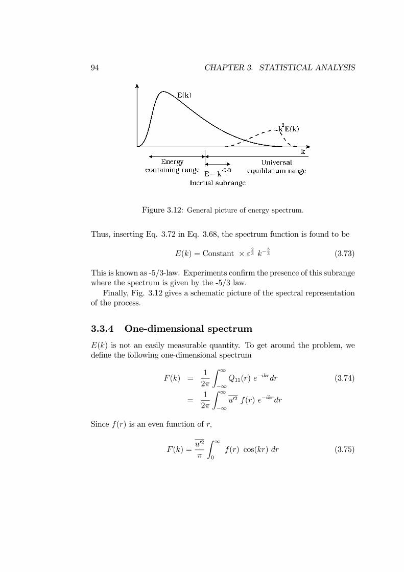
94 CHAPTER 3. STATISTICAL ANALYSIS
Figure 3.12: General picture of energy spectrum.
Thus, inserting Eq. 3.72 in Eq. 3.68, the spectrum function is found to be
E(k) = Constant × ε23 k−
53 (3.73)
This is known as -5/3-law. Experiments confirm the presence of this subrangewhere the spectrum is given by the -5/3 law.Finally, Fig. 3.12 gives a schematic picture of the spectral representation
of the process.
3.3.4 One-dimensional spectrum
E(k) is not an easily measurable quantity. To get around the problem, wedefine the following one-dimensional spectrum
F (k) =1
2π
∞
−∞Q11(r) e
−ikrdr (3.74)
=1
2π
∞
−∞u 2 f(r) e−ikrdr
Since f(r) is an even function of r,
F (k) =u 2
π
∞
0
f(r) cos(kr) dr (3.75)

3.3. SPECTRUM ANALYSIS 95
The inverse transform is
u 2f(r) = 2∞
0
F (k) cos(kr) dk (3.76)
It can be shown that, in isotropic turbulence, the one-dimensional spec-trum F (k) is related to the energy spectrum function E(k)
E(k) = k2F (k)− kF (k) (3.77)
(see for example Raudkivi and Callander, 1975, p.174).Incidentally, inserting Eq. 3.73 into Eq. 3.77 gives
ε23
k53
= k2F (k)− kF (k) (3.78)
This has a solution:
F (k) =9
55ε23k−
53 +
k2
2C1 + C2 (3.79)
The second and third terms on the right-hand-side of the preceding equationshould drop because F (k) should go to zero for large values of k, and therefore
F (k) = Constant× ε23k−
53 (3.80)
Example 8 The correlation function f(r) is approximated by
f(r) = exp(− r
Λf)
Find the one-dimensional and three-dimensional spectrum functions.
The one-dimensional spectrum function from Eq. 3.75
F (k) =u 2
π
∞
0
f(r) cos(kr) dr =Λf u 2
π(1 + (kΛf)2)
For k = 0:
k = 0 : F (0) =Λf u 2
π

96 CHAPTER 3. STATISTICAL ANALYSIS
Figure 3.13: 1-D and 3-D energy spectra for the numerical example.
Hence,
F (k) =F (0)
1 + (kΛf)2
(see Fig. 3.13 a).Regarding the three-dimensional energy spectrum function E(k), consid-
ering that the turbulence is isotropic, therefore using Eq. 3.77
E(k) = 8F (0)(kΛf)
4
(1 + (kΛf)2)3
(see Fig. 3.13 b for E(k)).
Example 9 One-dimensional spectrum function for a boundary layer in anopen channel.
Fig. 3.14 a shows the one-dimensional spectrum function obtained foran open channel flow by Raichlen (1967). (The results are normalized as

3.3. SPECTRUM ANALYSIS 97
Figure 3.14: 1-D energy spectra. (a): measured in an open channel. Raichlen(1967). (b): measured in a jet. Champagne (1978).

98 CHAPTER 3. STATISTICAL ANALYSIS
indicated in the figure. The Reynolds number is defined as Re = 4RVνin
which R is the hydraulic radius). Fig. 3.14 b, on the other hand, shows theone-dimensional spectrum measured in a jet.It may be noticed that, over a wave number interval, namely 1 < kh
2π< 6,
in Fig. 3.14 a, E(k) is apparently
E(k) ∼ k− 53
revealing the previously mentioned Kolmogoroff’s -5/3 law. The same holdstrue for the second example (Fig. 3.14 b) for the range 4×10⁻² cm−1 < k1 <10 cm−1.
3.4 References
1. Champagne, F.H. (1978): ”The fine-scale structure of the turbulentvelocity field”. Journal of Fluid Mechanics, Vol. 86, pp. 67-108.
2. Eckelman, H. (1974): ”The structure of the viscous sublayer and theadjacent wall region in a turbulent channel flow”. J. Fluid Mech., vol.65, p.439.
3. Hinze, J.O. (1959): Turbulence. McGraw-Hill.
4. Raichlen, F. (1967): ”Some turbulence measurements in water”. J.Eng. Mech. Proc. ASCE, p.73.
5. Raudkivi, A.J. and Callander, R.A. (1975). Advanced FluidMechanics.Edward Arnold.
6. Sumer, B.M. and Deigaard, R. (1981): ”Particle motions near the bot-tom in turbulent flow in an open channel - Part 2”. Journal of FluidMechanics, Vol. 109, pp. 311-337.
7. Sumer, B.M. and Oguz, B. (1978): ”Particle motions near the bottomin turbulent flow in an open channel”. Journal of Fluid Mechanics, Vol.86, pp. 109-127.

Chapter 4
Diffusion and dispersion
Diffusion/dispersion is another important property of turbulent flows. Someexamples are: (1) Waste products released into a recipient environment suchas a stream or the ocean undergo rapid diffusion; (2) Smoke (or exhaust gases)released into the atmosphere diffuses rapidly when there is strong wind; (3)Likewise, dredged material (sand, silt, etc.), when dumped into the sea, issubjected to large diffusion.The objective of this chapter is to describe the diffusion and dispersion
processes in turbulent flows. First, we will study the diffusion process in aturbulent flow field (a general analysis), and then, we will turn our atten-tion to the so-called longitudinal dispersion process, a process caused by thecombined action of the turbulent diffusion and the velocity variation in theflow.
4.1 One-Particle analysis
Release a lump of dispersant into the flow in the form of an instantaneouspoint source. The point of release is x = 0, and time t = 0 (Fig. 4.1). Thisdispersant will undergo diffusion as it is convected downstream, as sketchedin Fig. 4.1.(Note that we will use the term dispersant to refer to any kind of passive
quantity such as waste products, suspended sediment, heat, etc. Also notethat we assume that there is no interaction between the dispersant and theflow; the dispersant acts as a ”passive” quantity).The diffusion of the dispersant is caused by the following mechanism.
99

100 CHAPTER 4. DIFFUSION AND DISPERSION
Figure 4.1: Definition sketch.
The instantaneous point source is actually formed by many dispersantparticles. Since the flow is turbulent, each particle will follow a randompath. This will cause the particles to get farther and farther apart as theytravel (Fig. 4.2). The end result will be the continuous spreading (diffusion)of the dispersant, as sketched in Fig. 4.1.The diffusion of a passive quantity can be studied by adopting one of the
following two approaches.
1. Release the dispersant in the form of a lump at x = 0 and at time t = 0;and follow the cloud of the dispersant as it ”grows” and is convecteddownstream; or
2. Release one particle at x = 0 and at time t = 0, and follow its pathx = x(t); Repeat this exercise many times, and determine the statisticalproperties of x(t). This approach is called the one-particle analysis.
In the following paragraphs, the latter approach will be adopted.For simplicity, we shall study the process in one dimension.The particles are released at x = 0, at time t = 0. They follow ran-
dom paths x(t). The objective of the analysis is to determine the statisticalproperties of x(t). These statistical properties are (Fig. 4.3)
1. The mean value of x, namely x; this will give the mean position of thedispersing cloud as it is convected downstream.
2. The variance of x, namely (x− x)2; this will give a measure of thedegree of dispersion of the cloud.

4.1. ONE-PARTICLE ANALYSIS 101
Figure 4.2: Random paths of particles.
3. Other statistical moments; and
4. The probability density function (p.d.f.) of the particle position, namelyp(x). This quantity is proportional to the concentration, as will bedemonstrated later in the chapter.
Figure 4.3: One-dimensional diffusion.
The particle velocity (the Lagrangian velocity):
V =dx
dt(4.1)
102 CHAPTER 4. DIFFUSION AND DISPERSION
Integrating gives
x(t) =t
0
V (t ) dt (4.2)
Now, ensemble averaging gives the mean particle position (the position ofthe centroid of the particle cloud):
x(t) =t
0
V (t ) dt =t
0
V (t ) dt (4.3)
Here, the ensemble averaging is
φ =Nn=1 φnN
(4.4)
in which φ is any hydrodynamic quantity, φn the value of φ in one realiza-tion, and N the total number of realizations. (In the present context, onerealization is one release of particle).The variance, on the other hand, can be calculated in the following way.
Lety(t) = x(t)− x(t) (4.5)
Then, from Eq. 4.2
y(t) = x(t)− x(t) =t
0
V (t ) dt −t
0
V (t ) dt (4.6)
=t
0
[V (t )− V (t )] dt
The integrand here is the fluctuating part of the particle velocity
V = V − V (4.7)
Hence,
y(t) =t
0
V (t ) dt (4.8)
Differentiating y2(t) with respect to t
d
dty2(t) = 2 y
dy
dt(4.9)

4.1. ONE-PARTICLE ANALYSIS 103
and from Eq. 4.8
d
dty2(t) = 2 [
t
0
V (t ) dt ] V (t) (4.10)
= 2t
0
V (t ) V (t) dt
The integrand in the preceding equation, V (t ) V (t), recalling the Lagrangiancorrelation coefficient (Eq. 3.42):
V (t ) V (t) = V 2V (t )V (t)
V 2= RL(t− t ) V 2 (4.11)
Then,d
dty2(t) = 2 V 2
t
0
RL(t− t ) dt (4.12)
To summarize at this point,
1. The mean particle position is given by Eq. 4.3; and
2. The variance of the particle position is given by Eq. 4.12.
Now, we will continue with the analysis for the following two extremecases: (1) For small times (t TL); and (2) For large times (t TL) inwhich TL is the Lagrangian macro time scale defined by
TL =∞
0
RL(t) dt (4.13)
(Eqs. 3.42 and 3.43). Recall that Lagrangian macro time scale, TL, may beinterpreted as the time during which a coherent structure keeps its ”identity”/ coherence (Section 3.2.2).
4.1.1 Diffusion for small times
For small times (t TL), the fluid particle keeps its identity/coherence,meaning that the particle velocity will be pretty much the same as that atthe point where the particle starts its travel, namely at x = 0 at time t = 0.This velocity is the Eulerian velocity at x = 0:
V (t) V (t = 0) ≡ u(x = 0) (4.14)

104 CHAPTER 4. DIFFUSION AND DISPERSION
Now, the mean particle position, from Eq. 4.3:
x(t) =t
0
V (t ) dt =t
0
u(x = 0) dt = u(x = 0)t
0
dt = u(x = 0) t
(4.15)Regarding the variance, for small times (t TL), first of all, V 2
u 2(x = 0), and secondly, RL(t− t ) 1. Therefore, Eq. 4.12
d
dty2(t) = 2 u 2(x = 0) t
and integrating givesy2(t) = u 2(x = 0) t2 (4.16)
Now, assume that the flow/turbulence is homogenous. Then the statisti-cal properties of velocity should be invariant with respect to the position:
u(x = 0) ≡ u(x) = u = constant (4.17)
andu 2(x = 0) ≡ u 2(x) = u 2 = constant (4.18)
Thus, the mean particle position and the variance will be (from Eqs. 4.15,4.16, 4.17, 4.18)
x(t) = u t (4.19)
andy2(t) = u 2 t2 (4.20)
The p.d.f. of the particle position, on the other hand, will be the sameas that of the Eulerian velocity provided that u should be replaced with x
t.
4.1.2 Diffusion for large times
Mean and variance of particle position.For large times (t TL), the analysis will be developed further for the
following special case. Namely, the particle velocity is a stationary randomfunction (s.r.f.) of time.(The particle velocity is a s.r.f. of time if the probability density function
of particle velocity is invariant with respect to time, i.e.,
p[V (t)] ≡ p[V (t+ τ)] (4.21)

4.1. ONE-PARTICLE ANALYSIS 105
meaning that the statistical properties of the particle velocity such as themean V and the variance (V − V )2 = V 2 are time invariant. Homogeneityin space is equivalent to being stationary in time).First, consider the mean particle position. From Eq. 4.3 (taking V (t )
outside the integral because it is constant),
x(t) =t
0
V (t ) dt = V t (4.22)
The mean particle velocity should be equal to the Eulerian mean velocity,u. (The fact that the Lagrangian velocity is a stationary random functionof time requires the homogeneity in the Eulerian sense; therefore, V ≡ u).Hence,
x(t) = u t (4.23)
Next, consider the variance of the particle position. Eq. 4.12:
d
dty2(t) = 2 V 2
t
0
RL(t− t ) dt (4.24)
Change the notationξ = t− t (4.25)
then Eq. 4.24 will be
d
dty2(t) = 2 V 2
t
ξ=0
RL(ξ) dξ (4.26)
Integrating by parts gives
y2(t) = 2 V 2(t
ξ=0
RL(ξ) dξ) t− 2V 2t
ξ=0
ξRL(ξ) dξ (4.27)
For large times (t TL), t is so large that the integrals in the precedingequation converge (provided, of course, that the form of RL(ξ) is such thatthe integrals do converge). Furthermore, the second term on the right handside is small compared with the first term. Hence, for large times,
y2(t) = 2 V 2(t
ξ=0
RL(ξ) dξ) t (4.28)

106 CHAPTER 4. DIFFUSION AND DISPERSION
The integral for large times can be approximated to
t
ξ=0
RL(ξ) dξ∞
ξ=0
RL(ξ) dξ = TL (4.29)
(from Eq.4.13). Inserting the latter equation in Eq. 4.28, and also consideringthat V 2 is identically equal to u 2 (due to the fact that V (t) is a stationaryrandom function of time), the variance is obtained as
y2(t) = 2 u 2TL t (4.30)
(As will be detailed in the following paragraphs, this is diffusion becausey2(t) ∼ t).To summarize, the mean particle position and the variance are given by
Eqs. 4.23 and 4.30, respectively.As seen from Eqs. 4.20 and 4.30, the variance is
y2(t) ∼ t2 for small times (t TL) (4.31)
andy2(t) ∼ t for large times (t TL) (4.32)
This implies that the spreading occurs very fast in the beginning of theprocess (y2(t) ∼ t2), and then the rate at which the spreading occurs reachesan equilibrium stage where y2(t) ∼ t, as sketched in Fig. 4.4.P.d.f. of particle position.The particle displacement (Eq. 4.2)
x(t) =t
0
V (t ) dt
can be considered as the sum of a series integral over a fixed interval, say τ ,
x(t) =t
0
V (t ) dt =n
(n+1)τ
nτ
V (t ) dt (4.33)
such that each integral has only a partial statistical connection with eachother. For times t TL, the number of such integrals becomes sufficientlylarge so that we have a situation like that covered by the central limit theo-rem.

4.1. ONE-PARTICLE ANALYSIS 107
Figure 4.4: Variance of particle position.
The central limit theorem states that for a series of statistically indepen-dent terms, the p.d.f. of the sum tends to the Gaussian distribution (normaldistribution), as the number of terms approaches infinity, irrespective of theprobability distributions of each term, which form the sum.Therefore, for large times t TL, the p.d.f. of x(t) will be
p(x) =1
√2π (x− x)2
exp(− (x− x)2
2(x− x)2) (4.34)
or, for convenience, changing the notation to y = x− x,
p(y) =1
√2π y2
exp(− y2
2 y2) (4.35)
Inserting Eq. 4.30 in the preceding equation,
p(y) =1
√2π 2 u 2TL t
exp(− y2
2 (2 u 2TL t)) (4.36)
We shall return to this equation later in the section.Now, consider the diffusion equation
∂c
∂t= D
∂2c
∂y2(4.37)

108 CHAPTER 4. DIFFUSION AND DISPERSION
in which D is the diffusion coefficient, y the space coordinate, and t the time.Consider the initial condition
t = 0 : c = δ(y) (4.38)
in which δ(y) is the Dirac delta function, which is defined by
δ(y) = 0 for y = 0
δ(y) = ∞ for y = 0
and ∞
−∞δ(y)dy = 1
The solution to the diffusion equation with the above initial condition is
c(y) =1√
2π√2Dt
exp(− y2
2 (2 D t)) (4.39)
Now, compare the above equation with Eq. 4.36. From this comparison,the following deductions can be made:
1. The p.d.f. of the particle position for large times (t TL) satisfies thediffusion equation (cf., 4.37)
∂p
∂t= D
∂2p
∂y2(4.40)
2. The diffusion coefficient of the diffusion process is
D = u 2TL (4.41)
which can, from Eq. 4.30, also be written as
D = u 2TL =1
2
dy2(t)
dt(4.42)
D is called the turbulent diffusion coefficient.
The theory summarized in the preceding paragraphs was developed byG.I. Taylor (1921). It was later extended to the three-dimensional case

4.1. ONE-PARTICLE ANALYSIS 109
by Batchelor (1949). For further reading, consult Batchelor and Townsend(1956) and Monin and Yaglom (1973).
Flux due to turbulent diffusion.The probability that a particle is present in the interval (y, y + dy)
Pr[y < Y < y + dy] =m
M(4.43)
where M is the total number of released particles, and m is the number ofparticles occupying the interval (y, y + dy).This probability can also be written as
Pr[y < Y < y + dy] = p(y) dy (4.44)
From the preceding two equations, one gets
p(y) =1
M
m
dy(4.45)
Here, mdy, the number of particles per unit length, is the concentration c in
the one-dimensional case. So,
p(y) =c(y)
M(4.46)
Now, the probability that a particle is present in the half space (−∞, y)is
Pr[−∞ < Y < y] =m1
M(4.47)
in which m1 is the number of particles occupying the interval (−∞, y). Like-wise, this probability can be written as
Pr[−∞ < Y < y] =y
−∞p(y) dy (4.48)
Then from Eqs. 4.47 and 4.48
m1 =My
−∞p(y) dy (4.49)
Differentiate the above equation with respect to time
−∂m1
∂t= −M ∂
∂t
y
−∞p(y) dy (4.50)

110 CHAPTER 4. DIFFUSION AND DISPERSION
Figure 4.5: Flux due to turbulent diffusion.
Here −∂m1
∂tis the rate of change in the number of the particles which occupy
the region (−∞, y), i.e., the decrease in the number of particles in the region(−∞, y) per unit time. This means that there is a continuous supply ofparticles from the region (−∞, y) to the region (y,+∞) at a rate −∂m1
∂t, i.e.,
the number of particles passing through the section y per unit time is −∂m1
∂t.
The expression for p(y) is given in Eq. 4.35. Substituting this equation inEq. 4.50, and integrating and then differentiating with respect to time gives
−∂m1
∂t=M
y
2tp(y) (4.51)
Differentiating Eq. 4.35 with respect to y, on the other hand, gives
∂p
∂y= − y
2Dtp(y) (4.52)
From the preceding two equations,
−∂m1
∂t= −MD∂p
∂y
or
−∂m1
∂t= −D∂(Mp)
∂y(4.53)
From Eq. 4.46, c =Mp. Inserting this in the above equation gives
−∂m1
∂t= −D ∂c
∂y(4.54)
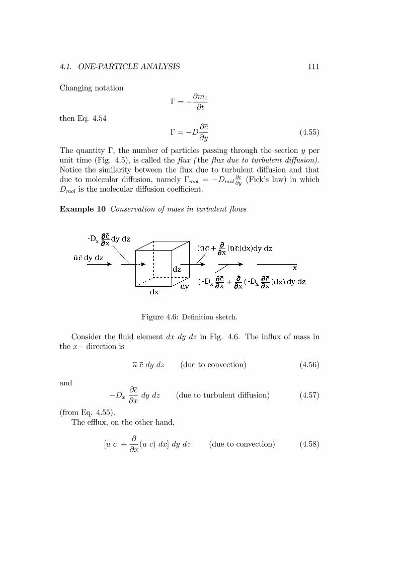
4.1. ONE-PARTICLE ANALYSIS 111
Changing notation
Γ = −∂m1
∂t
then Eq. 4.54
Γ = −D ∂c
∂y(4.55)
The quantity Γ, the number of particles passing through the section y perunit time (Fig. 4.5), is called the flux ( the flux due to turbulent diffusion).Notice the similarity between the flux due to turbulent diffusion and thatdue to molecular diffusion, namely Γmol = −Dmol ∂c∂y (Fick’s law) in whichDmol is the molecular diffusion coefficient.
Example 10 Conservation of mass in turbulent flows
Figure 4.6: Definition sketch.
Consider the fluid element dx dy dz in Fig. 4.6. The influx of mass inthe x− direction is
u c dy dz (due to convection) (4.56)
and
−Dx∂c
∂xdy dz (due to turbulent diffusion) (4.57)
(from Eq. 4.55).The efflux, on the other hand,
[u c +∂
∂x(u c) dx] dy dz (due to convection) (4.58)

112 CHAPTER 4. DIFFUSION AND DISPERSION
and
[−Dx∂c
∂x+
∂
∂x(−Dx
∂c
∂x) dx] dy dz (due to turbulent diffusion) (4.59)
Thus the net influx in the x− direction is
− ∂
∂x(u c) dx dy dz − ∂
∂x(−Dx
∂c
∂x) dx dy dz (4.60)
Similar expressions for the y− and z− directions:
− ∂
∂y(v c) dx dy dz − ∂
∂y(−Dy
∂c
∂y) dx dy dz (4.61)
− ∂
∂z(w c) dx dy dz − ∂
∂z(−Dz
∂c
∂z) dx dy dz (4.62)
On the other hand, the rate of change of mass in the volume dx dy dz
∂
∂t(c dx dy dz) (4.63)
The conservation of mass requires that the rate of change of mass shouldbe equal to the net influx. Hence, from Eqs. 4.60-4.63, and using the conti-nuity equation (Eq. 1.6), namely
∂u
∂x+
∂v
∂y+
∂w
∂z= 0 (4.64)
one gets
∂c
∂t+ u
∂c
∂x+ v
∂c
∂y+ w
∂c
∂z=
∂
∂x(Dx
∂c
∂x) +
∂
∂y(Dy
∂c
∂y) +
∂
∂z(Dz
∂c
∂z) (4.65)
or, in index notation
∂c
∂t+ ui
∂c
∂xi=
∂
∂xi(Di
∂c
∂xi) (4.66)
and including the molecular diffusion effect as well
∂c
∂t+ ui
∂c
∂xi=
∂
∂xi(Di +Dmol)
∂c
∂xi) (4.67)
However, note that, normally, Dmol Di.

4.2. LONGITUDINAL DISPERSION 113
4.2 Longitudinal dispersion
4.2.1 Mechanism of longitudinal dispersion
The mechanism of longitudinal dispersion may be best described by referenceto an open-channel flow, Fig. 4.7. Release a lump of dispersant in the formof a point source at section x = 0 and t = 0. Consider that the releaseddispersant is formed by many particles. Now, these particles are subject totwo effects:
1. The turbulent motion in the y− direction; Under this effect, the parti-cles travel up and down in a random fashion.
2. The streamwise motion in the x− direction. The particles take thevelocity u(y), plus a small fluctuating velocity u . (However, the latteris negligible with respect to the former).
Figure 4.7: Longitudinal dispersion.

114 CHAPTER 4. DIFFUSION AND DISPERSION
Particles near the bottomwill experience relatively smaller velocities u(y),and therefore will be retarded (Path 1 in Fig. 4.7 a) while particles near thefree surface will experience relatively larger velocities u(y), and thereforewill be moved large distances (Path 2 in Fig. 4.7 a). This implies that theparticles are prone to disperse farther and farther apart in the streamwisedirection. Thus, the end result will be the progressive dispersion of thedispersant in the streamwise direction, as sketched in Fig. 4.7 b. This processis called the longitudinal dispersion.When compared with the ordinary diffusion process studied in the previ-
ous section (cf., Fig. 4.1 and 4.2), the key effect here is that the dispersion iscaused mainly by the velocity variation u(y) across the depth, whereas thedispersion in the ordinary diffusion process is caused by the random paths ofparticles; no spatial variation in the mean velocity exists in the latter process.For the above reason, the present diffusion process is sometimes called
the mechanical dispersion.From the preceding considerations, it can easily be seen that
1. there will be no longitudinal dispersion, when the velocity distributionacross the depth is uniform; and
2. likewise, there will be no longitudinal dispersion when there is no turbu-lent motion across the depth (i.e., when there is no turbulent diffusionacross the depth). (Note, however, that the existing molecular diffu-sion will cause longitudinal dispersion although the degree of dispersionin this case is several orders of magnitude smaller than the turbulentlongitudinal dispersion, Taylor, 1953, 1954, Elder, 1959).
4.2.2 Application of one-particle analysis
Fig. 4.8 shows the path of a particle. Here, V (t) is the streamwise velocityof the particle. V (t) is actually the sum of two velocities:
1. the velocity u(y) at the position where the particle is at that particulartime t, and
2. the x− component of the fluctuating velocity u , which occurs at thatposition, and at that particular time, t.
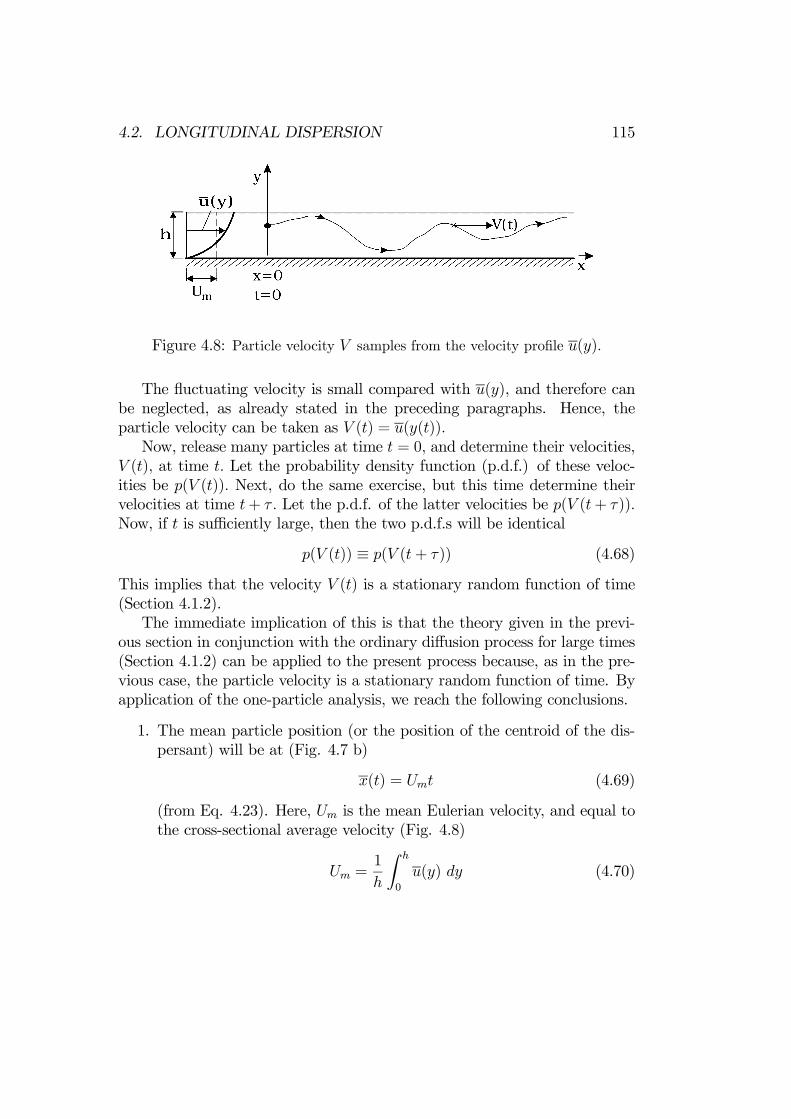
4.2. LONGITUDINAL DISPERSION 115
Figure 4.8: Particle velocity V samples from the velocity profile u(y).
The fluctuating velocity is small compared with u(y), and therefore canbe neglected, as already stated in the preceding paragraphs. Hence, theparticle velocity can be taken as V (t) = u(y(t)).Now, release many particles at time t = 0, and determine their velocities,
V (t), at time t. Let the probability density function (p.d.f.) of these veloc-ities be p(V (t)). Next, do the same exercise, but this time determine theirvelocities at time t+ τ . Let the p.d.f. of the latter velocities be p(V (t+ τ)).Now, if t is sufficiently large, then the two p.d.f.s will be identical
p(V (t)) ≡ p(V (t+ τ)) (4.68)
This implies that the velocity V (t) is a stationary random function of time(Section 4.1.2).The immediate implication of this is that the theory given in the previ-
ous section in conjunction with the ordinary diffusion process for large times(Section 4.1.2) can be applied to the present process because, as in the pre-vious case, the particle velocity is a stationary random function of time. Byapplication of the one-particle analysis, we reach the following conclusions.
1. The mean particle position (or the position of the centroid of the dis-persant) will be at (Fig. 4.7 b)
x(t) = Umt (4.69)
(from Eq. 4.23). Here, Um is the mean Eulerian velocity, and equal tothe cross-sectional average velocity (Fig. 4.8)
Um =1
h
h
0
u(y) dy (4.70)

116 CHAPTER 4. DIFFUSION AND DISPERSION
2. The variance will be
(x− x)2 = 2 V 2TL1 t (4.71)
(from Eq. 4.30). Here TL1 is the Lagrangian time scale defined by
TL1 =∞
0
RL1(t) dt (4.72)
in which RL1(t) is the Lagrangian correlation coefficient
RL1(t) =V (τ)V (τ + t)
V 2(4.73)
in whichV = V − Um (4.74)
Here, the subindex 1 is used to distinguish the present application fromthe ordinary diffusion.
3. The p.d.f. of the particle position tends to the Gaussian (normal)distribution for large times (t TL1):
p(x) =1
√2π (x− x)2
exp(− (x− x)2
2(x− x)2) (4.75)
(from Eq. 4.34).
4. The diffusion coefficient of the process is
D1 = V 2TL1 =1
2
d(x− x)2dt
(4.76)
(from Eq. 4.42). Here, D1 is called the longitudinal dispersion coeffi-cient.
5. The p.d.f. of particle position satisfies the diffusion equation
∂p
∂t= D1
∂2p
∂(x− x)2 (4.77)

4.2. LONGITUDINAL DISPERSION 117
(from Eq. 4.40). Here, ∂∂tis the time derivative when considering the
moving coordinate x− x(t). Changing to the fixed coordinate x,
∂
∂t=
∂
∂t+
∂
∂x
∂x
∂t=
∂
∂t+
∂x(t)
∂t
∂
∂x=
∂
∂t+ Um
∂
∂x(4.78)
Then, Eq. 4.77 becomes
∂p
∂t+ Um
∂p
∂x= D1
∂2p
∂x2(4.79)
6. From Eqs. 4.79 and 4.46
∂ < c >
∂t+ Um
∂ < c >
∂x= D1
∂2 < c >
∂x2(4.80)
in which < c > is the cross-sectional average concentration:
< c >=1
h
h
0
c dy (4.81)
Eq. 4.80 is called the dispersion equation.
The above analysis shows that the longitudinal dispersion process is rep-resented by a one-dimensional diffusion equation with constant coefficientsUm and D1 (Eq. 4.80). The process is also governed by the general diffusionequation (Eq. 4.65):
∂c
∂t+ u
∂c
∂x+ v
∂c
∂y=
∂
∂x(Dx
∂c
∂x) +
∂
∂y(Dy
∂c
∂y) (4.82)
Clearly, the one-dimensional equation (Eq. 4.80) is much simpler than thetwo-dimensional representation (Eq. 4.82). (This is the advantage of thelongitudinal-dispersion concept). Obviously, this is at the expense of thecalculated concentration. In the one-dimensional representation, the cross-sectional average concentration is calculated, whereas, in the two-dimensionalrepresentation, the point-concentration is calculated. However, this is not aproblem, because, in longitudinal-dispersion problems, the calculation withthe cross-sectional average concentration is normally good enough (the con-centration variations in the longitudinal direction are important, not thevariations over the cross section).

118 CHAPTER 4. DIFFUSION AND DISPERSION
For the application of the previously mentioned one-dimensional disper-sion equation, two quantities need to be known: the cross-sectional averagevelocity, Um, and the longitudinal dispersion coefficient, D1.
Um is obtained simply by integrating the velocity distribution over thecross-section, and dividing it by the cross-sectional area. This is done ifthe velocity distribution is known theoretically (for ex., in the form of thelogarithmic law). Otherwise, the velocity distribution over the cross-sectionis measured, for example, as in the case of a natural stream, and the meanvelocity calculation is based on the measured velocity.
The longitudinal dispersion coefficient, on the other hand, can be calcu-lated theoretically (see the next section), or it can be calculated numerically,based on the measured velocity distribution over the cross section, as will bedetailed in Section 4.4.
G.I. Taylor (1953, 1954) introduced the concept of the longitudinal disper-sion. In his study, the flow environment was a circular pipe. His theoreticalwork and his experiments showed that the longitudinal dispersion coefficientin a turbulent pipe flow (Taylor, 1954) is D1
aUf= 10 in which a is the radius of
the pipe, and Uf is the friction velocity. Taylor’s work laid the groundworkfor the later research in 1960s and 70s in the area of dispersion in naturalstreams, estuaries, etc. and also in industrial flows (such as pipe flows).
4.3 Calculation of dispersion coefficient
In this section, we shall calculate the longitudinal dispersion coefficient foran open channel flow (Fig. 4.7). We shall do this exercise for heavy particles(for example, sand, or silt in water). This feature will be represented by thefall velocity of the particles, w. However, the case of the neutrally-buoyantparticles/dispersant will be captured by setting w equal to zero in the endsolutions.
The analysis presented in the following paragraphs is mainly based on thework of Sumer (1974). It may be noted that the method used in the analysiswas first introduced by Aris (1956) and also employed by Sayre (1968).

4.3. CALCULATION OF DISPERSION COEFFICIENT 119
4.3.1 Formulation
The conservation of mass (Fig. 4.7) from Eq. 4.65:
∂c
∂t+ u(y)
∂c
∂x− w ∂c
∂y=
∂
∂x( (y)
∂c
∂x) +
∂
∂y( (y)
∂c
∂y) (4.83)
in which w is the fall velocity of the particles, and (y) is the turbulentdiffusion coefficient. It is assumed that (y) is the same for both x− and y−directions.The boundary conditions:
y = 0 and h: (y)∂c
∂y+ wc = 0 (4.84)
implying that there is no net transport across the boundaries.The initial condition is (for a uniformly distributed plane source)
t = 0: c(x, y, 0) =M
hδ(x) (4.85)
in which M is the total number of particles released into the flow.Furthermore, we write
u(y) = Um(1 + χ(y)), and (y) = Dmψ(y) (4.86)
in which Um and Dm are the cross-sectional average velocity and the cross-sectional average diffusion coefficient, respectively. We shall return to thesequantities and the nondimensional functions χ(y) and ψ(y) later in the sec-tion.Now, define the pth moment of concentration
Cp =∞
−∞ξpCdξ (4.87)
in which ξ is the normalized streamwise distance defined by
ξ =x− Usth
(4.88)
in which Us is the mean particle velocity, and C is the normalized concen-tration defined by
C =cMh2
(4.89)

120 CHAPTER 4. DIFFUSION AND DISPERSION
Now, multiply the two sides of the above equations (Eqs. 4.83-4.85) byξp, and integrate the equations from −∞ to +∞:
∂Cp∂τ− (μ− μs + μχ)pCp−1 − νs
∂Cp∂η
= p(p− 1)ψCp−2 +∂
∂η(ψ
∂Cp∂η) (4.90)
η = 0 and 1: ψ∂Cp∂η
+ νsCp = 0 (4.91)
and
τ = 0: Cp(η, 0) = 1 and 0, respectively, for p = 0 and p > 0 (4.92)
Here,
η =y
h, τ =
Dmt
h2(4.93)
are the normalized distance from the bottom of the channel and the nor-malized time, respectively. Also, μ, μs and νs are the normalized mean flowvelocity, the normalized mean particle velocity and the normalized mean fallvelocity, respectively:
μ =Umh
Dm, μs =
Ush
Dm, νs =
wh
Dm(4.94)
Regarding the flow velocity, u(y), and turbulent diffusion coefficient, (y),distributions across the depth, first of all, from Eq. 2.85,
u− Um =1
κUf [ln(
y
h) + 1] (4.95)
(the logarithmic law). The distribution of the turbulent diffusion coefficient,on the other hand, is found from the analogy between the momentum flux(Eq. 2.89) and the flux due to turbulent diffusion
=−Γdcdy
=−ρu vρdudy
(4.96)
Taking −ρu v ρU2f (1 − yh) (see Eq. 2.21), and using the above analogy
(Eq. 4.96), the diffusion coefficient
(y) = κUf y(1−y
h) (4.97)

4.3. CALCULATION OF DISPERSION COEFFICIENT 121
and Dm is
Dm =1
h
h
0
(y) dy =1
6κhUf (4.98)
The functions χ(y) and ψ(y) in Eqs. 4.86 are then
μχ =6
κ2(1 + ln η), and ψ = 6η(1− η) (4.99)
4.3.2 Zeroth moment of concentration
For p = 0, the solution to the Eqs. 4.90-4.92 is found to be as follows
C0 =sin(πβ)
πβ(1− η
η)β+
∞
K=1
aK(1− η
η)βF (−K, 1+K; 1−β; η) exp−6(K2+K)τ
(4.100)in which aK
aK =(2K + 1) Γ(K + 1− β)
Γ2(1− β) Γ(K + 1 + β)3F2(−K,K + 1, 1; 1− β, 2; 1) (4.101)
F is a hypergeometric function, 3F2 is a generalized hypergeometric series,and Γ is the Gamma function (Gradshteyn and Ryzhik, 1965). The quantityβ here is the fall velocity parameter defined by
β =νs6=
w
κUf(4.102)
and the solution is found for β = 0, β < 1.Fig. 4.9 displays C0(η, τ) for two values of β. Note that the physical
meaning of C0 is that C0 is identical to the p.d.f. of the particle positionacross the depth. As seen from the figure, the larger the value of β, the moreweighted the distributions towards the bottom, as expected.From Eq. 4.100
C0(η) =sin(πβ)
πβ(1− η
η)β as τ →∞ (4.103)
Sumer (1974) argues that, for the case of neutrally buoyant particles (β = 0),C0 should go to unity, C0 → 1. Indeed the above equation reveals this.

122 CHAPTER 4. DIFFUSION AND DISPERSION
Figure 4.9: C0(η, τ) for two different sediment with (a): β = wκUf
= 0.1, and (b):
β = wκUf
= 0.3. Sumer (1974).
4.3. CALCULATION OF DISPERSION COEFFICIENT 123
4.3.3 Mean particle velocity
For this, we define
mp =1
0
Cp dη (4.104)
Now, integrate Eqs. 4.90 and 4.92 from η = 0 to 1, and using the boundaryconditions (Eq. 4.91),
dmp
dτ− p
1
0
(μ− μs + μχ)Cp−1 dη − p(p− 1)1
0
ψCp−2 dη = 0 (4.105)
τ = 0: mp(0) = 1 and 0, respectively, for p = 0 and p > 0 (4.106)
Now, the preceding two equations for p = 1
dm1
dτ−
1
0
(μ− μs + μχ)C0 dη = 0 (4.107)
andm1(0) = 0 at τ = 0 (4.108)
Note that m1 represents the mean particle displacement relative to the ξaxis, and dm1
dτrepresents the mean particle velocity relative to this axis. Since
this axis moves with the mean particle velocity (Eq. 4.88), then dm1
dτ→ 0 as
time τ →∞. Hence, from Eq. 4.107, for large times
−1
0
(μ− μs + μχ)C0(η,∞) dη = 0
or, from Eq. 4.103,
μs − μ =1
0
μχ C0(η,∞) dη =1
0
μχsin(πβ)
πβ(1− η
η)β dη (4.109)
This is the mean particle velocity relative to the mean flow velocity. Fig.4.10 illustrates how the mean particle velocity varies with the fall velocityparameter. Note that for β = 0, the case of neutrally-buoyant particles,obviously this velocity must be equal to the mean flow velocity, meaningthat μs − μ must be zero, as revealed by the figure.

124 CHAPTER 4. DIFFUSION AND DISPERSION
Figure 4.10: Mean velocity of heavy particles relative to the mean flow velocity.Sumer (1974).
4.3.4 Longitudinal dispersion coefficient
The longitudinal dispersion coefficient can be written in the normalized formas
D1hUf
=κ6(1
2
dm2
dτ)τ→∞ (4.110)
(see Eqs. 4.87 and 4.104).From Eq. 4.105,
1
2
dm2
dτ= 6
1
0
η(1− η)C0 dη +1
0
(μ− μs + μχ)C1 dη (4.111)

4.3. CALCULATION OF DISPERSION COEFFICIENT 125
in which C1 is found from Eqs. 4.90-4.92, setting p = 1
C1 = φ(η) +∞
K=1
aKfK(η) exp−6(K2 +K)τ (4.112)
+∞
K=1
dK(1− η
η)βF (−K, 1 +K; 1− β; η) exp−6(K2 +K)τ
in which
φ = Aφ(1− η
η)β − sin(πβ)
πβ(1− η
η)β
η
0
(1− η
η)−β
1
6η(1− η)dη(4.113)
×η
0
(μ− μs + μχ)(1− η
η)βdη
in which β < 1. It may be noted that C1 → φ as τ →∞.Now, from Eqs. 4.111, 4.113 and 4.103, the dispersion coefficient is ob-
tained as
D1hUf
=κ6(1− β2)− κ
36
sin(πβ)
πβ
1
0
[(μ− μs) + μχ](1− η
η)βdη (4.114)
×η
0
(1− η
η)−β
1
η(1− η)dη
η
0
[(μ− μs) + μχ](1− η
η)βdη
in which β < 1.For the case of neutrally buoyant particles/dispersant, putting β = 0, one
getsD1hUf
=κ6− κ36
1
0
μχdηη
0
1
η(1− η)dη
η
0
μχdη (4.115)
The expression in Eq. 4.115 was first obtained by Elder (1959). The integralcan be calculated numerically. The result is (taking κ, the von Karmanconstant, 0.41)
D1hUf
= 0.07 + 5.86 = 5.93 (4.116)
As seen from Eq. 4.115, the dispersion coefficient consists of two terms; thefirst term on the right hand side of the equation, κ
6, (the numerical value of
which is 0.07, Eq. 4.116) represents the effect of the turbulent diffusion inthe streamwise direction; it stems from the first term on the right hand sideof Eq. 4.83. The second term is actually the main portion of the longitudinal

126 CHAPTER 4. DIFFUSION AND DISPERSION
Figure 4.11: Ratio of the longitudinal dispersion coefficient of heavy particles tothat of neutrally-buoyant particles. Sumer (1974).
dispersion coefficient, and induced by the combined action of the turbulentdiffusion across the depth y and the variation of the flow velocity in the y−direction.Returning to the case of heavy particles, the dispersion coefficient is plot-
ted in Fig. 4.11. The figure shows that the dispersion coefficient increaseswith increasing β, the fall velocity parameter. This can be explained as fol-lows. A heavy particle spends most of the time near the bottom where thevelocity gradient is largest. On the other hand, the larger the velocity gra-dient, the larger the dispersion coefficient. Therefore, a heavier particle (i.e.,with larger β) should have a larger dispersion coefficient.
4.4 Longitudinal dispersion in rivers
In the previous section, the longitudinal dispersion coefficient has been calcu-lated for an open-channel flow, and found to be D1
hUf6. Field experiments in

4.4. LONGITUDINAL DISPERSION IN RIVERS 127
Figure 4.12: (a): The cross-sectional velocity distribution at Renton Junction inthe Green-Duwamish River, Washington. Contours are lines of constant velocity,in increment of 0.2 ft/s; (b): The transverse profile of the depth-averaged velocitycorresponding to the velocity distribution shown in (a). Taken from Fischer et al.(1979).
rivers show, however, that D1hUf
takes values much larger than 6. The largest
value reported in Fischer et al. (1979) is D1hUf
7500 in the Missouri river.This evidence makes it clear that the value obtained for the case of the openchannel, namely D1
hUf6, cannot apply to real streams. The reason why
D1hUf
6 value does not apply was studied by Fischer (1966, 1967). It wasshown that, in the case of real streams, although the velocity distributionsatisfies the logarithmic law in the vertical direction, the variation of thevelocity across the river width apparently plays the major role.A quantitative estimate of the dispersion coefficient in a real stream can be
obtained by neglecting the vertical profile completely, but instead, by taking

128 CHAPTER 4. DIFFUSION AND DISPERSION
the transverse velocity profile, i.e., the velocity profile across the river width.(Fig. 4.12 displays an example illustrating the transverse velocity variation ina river, the velocity isolines at a measurement section in the Green-DuwamishRiver in Washington, and the corresponding transverse velocity profile).Fisher obtained the following expression for the longitudinal dispersion
coefficient
D1 = −1
A
W
0
(u(y)− Um) d(y) dyy
0
1
td(y)dy
y
0
(u(y)− Um) d(y) dy(4.117)
in which A is the cross-sectional area of the river, W width at the surface,Um mean flow velocity, y the transverse distance measured from one bankof the river (Fig. 4.12) (not to be confused with the vertical distance usedin the previous section), d(y) the depth (the depth is a function of y, Fig.4.12), t is the turbulent diffusion coefficient in the transverse direction (itmay or may not be a function of y), and u(y) is the depth-averaged velocitydefined by (Fig. 4.12) :
u(y) =1
d(y)
0
−d(y)u(y, z) dz (4.118)
Returning to the expression obtained for the case of the open-channelflow in the previous section, Eq. 4.115, (omitting the first term on the righthand side of the equation)
D1hUf
= − κ36
1
0
μχdηη
0
1
η(1− η)dη
η
0
μχdη
This is actually in terms of dimensional quantities
D1hUf
= −1h
h
0
(u(y)− Um)dyy
0
1
(y)dy
y
0
(u(y)− Um)dy
or alternatively
D1hUf
= − 1h2
h
0
(u(y)− Um)hdyy
0
1
(y)hdy
y
0
(u(y)− Um)hdy (4.119)
As seen, this expression is quite similar to that obtained by Fischer (1966,1967), Eq. 4.117. The only difference is that, in the case of the river dis-persion, y is the transverse distance, while, in the case of the open-channeldispersion, y is the vertical distance.

4.5. REFERENCES 129
Fischer et al. (1979) give a numerical example to illustrate how to useEq. 4.117 in a field application.Finally, it may be noted that real streams may have irregularities such as
bends, sandbars, side pockets, pools, riffles, bridge piers, man-made revet-ments, and even occasional junked car, or sunken barges. Every irregularitycontributes to dispersion. (Fischer et al., 1979, and Pedersen, 1977). Empir-ical expressions have been given for the longitudinal dispersion coefficient interms of gross flow characteristics of the river (Fischer et al., 1979, p. 136).These can be used to make first assessments of the dispersion coefficient.
4.5 References
1. Aris, R. (1956): ”On the dispersion of a solute in a fluid flowing througha tube”. Proc. Roy. Soc., vol. A235, p. 67.
2. Batchelor, G.K. (1949): ”Diffusion in a field of homogenous turbu-lence”. Australian J. Sci. Res., vol. A2, No. 4, p.473.
3. Batchelor, G.K. and Townsend, A.A. (1956):”Turbulent diffusion”. In:Surveys in Mechanics (ed. G.K. Batchelor and R. M Davies), Cam-bridge University Press, p.352.
4. Elder, J. (1959): ”The dispersion of marked fluid in turbulent shearflow”. J. Fluid Mech.., vol. 5, p. 544.
5. Fischer, H.B. (1966): Longitudinal Dispersion in Laboratory and Nat-ural Streams. Tech. Report KH-R-12, California Institute of Technol-ogy, Pasadena, California.
6. Fischer, H.B. (1967): ”The mechanics of dispersion in natural streams”.J. Hydraul. Div., Proc. ASCE, vol. 93, p. 187.
7. Fischer, H.B., List, E.J., Koh, R.C.Y., Imberger, J. and Brooks, N.H.(1979): Mixing in Inland and Coastal Waters. Academic Press, Inc.
8. Monin, A.M. and Yaglom, A.S. (1973): Statistical Fluid Mechanics:Mechanics of Turbulence, vol. 1, MIT Press. Cambridge, Mass.

130 CHAPTER 4. DIFFUSION AND DISPERSION
9. Pedersen, F.B. (1977): Prediction of Longitudinal Dispersion in Nat-ural Streams. Series Paper No. 14, Technical University of Denmark,Institute of Hydrodyn. and Hyd. Eng. (ISVA).
10. Sayre, W.W. (1968): Hydraulic Papers, No. 3, Colorado State Univer-sity, Fort Collins.
11. Sumer, B.M. (1974): ”Mean velocity and longitudinal dispersion ofheavy particles in turbulent open-channel flow”. J. Fluid Mech., vol.65, p.11.
12. Taylor, G.I. (1921): ”Diffusion by continuous movements”. Proc. Lon-don Math. Soc., vol. 20, p. 196.
13. Taylor, G.I. (1953): ”Dispersion of soluble matter in solvent flowingslowly through a tube”. Proc. Roy. Soc. London, A, vol. CCXIX,p.186.
14. Taylor, G.I. (1954): ”The dispersion of matter in turbulent flow througha pipe”. Proc. Roy. Soc. London, vol. A223, p.446.

Chapter 5
Wave boundary layers
In shallow waters, the orbital motion of water particles under a progressivewave degenerates into a bottom-parallel, straight line, oscillatory motion atthe seabed (Fig. 5.1). For each half cycle of this oscillatory motion at thebed, a ”new” time-dependent boundary layer develops. This cyclic boundarylayer is called the wave boundary layer.
The wave boundary layers are of great importance for several processes:Turbulent mixing of mass and momentum takes place in the wave bound-ary layers; Likewise, frictional dissipation takes place in the wave boundarylayers; The wave boundary layers are one of the key components of the sed-iment transport processes; Exchanges of chemicals and organisms betweenseabed and the main body of the water take place in the wave boundary lay-ers. Therefore, understanding of wave-boundary layers is essential to developpredictive tools and capabilities for the previously mentioned processes.
Fredsøe and Deigaard (1992, Chapters 2 and 3) can be consulted for adetailed treatment of the subject including the mathematical modelling.
The flow in the wave boundary layers may be in the laminar regime, itmay be in the transitional, or it may be in the turbulent regime.
We will start off with the laminar-regime wave boundary layers, and thenwe will focus on the turbulent wave boundary layers. The latter will bemainly based on the work of Jensen et al. (1989), an extensive experimen-tal work conducted in an oscillating water tunnel, covering both smooth-and rough-boundary flows, with very broad range of the Reynolds numberincluding very high Reynolds numbers.
131
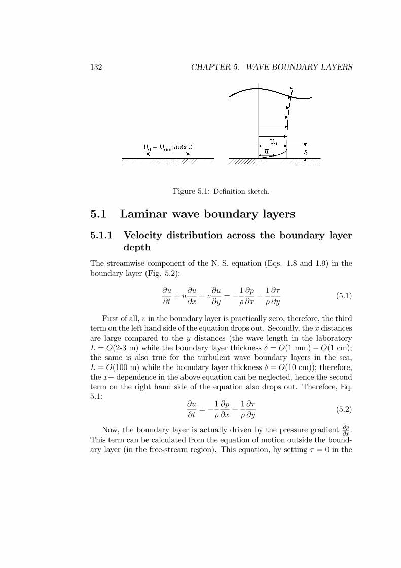
132 CHAPTER 5. WAVE BOUNDARY LAYERS
Figure 5.1: Definition sketch.
5.1 Laminar wave boundary layers
5.1.1 Velocity distribution across the boundary layerdepth
The streamwise component of the N.-S. equation (Eqs. 1.8 and 1.9) in theboundary layer (Fig. 5.2):
∂u
∂t+ u
∂u
∂x+ v
∂u
∂y= −1
ρ
∂p
∂x+1
ρ
∂τ
∂y(5.1)
First of all, v in the boundary layer is practically zero, therefore, the thirdterm on the left hand side of the equation drops out. Secondly, the x distancesare large compared to the y distances (the wave length in the laboratoryL = O(2-3 m) while the boundary layer thickness δ = O(1 mm)−O(1 cm);the same is also true for the turbulent wave boundary layers in the sea,L = O(100 m) while the boundary layer thickness δ = O(10 cm)); therefore,the x− dependence in the above equation can be neglected, hence the secondterm on the right hand side of the equation also drops out. Therefore, Eq.5.1:
∂u
∂t= −1
ρ
∂p
∂x+1
ρ
∂τ
∂y(5.2)
Now, the boundary layer is actually driven by the pressure gradient ∂p∂x.
This term can be calculated from the equation of motion outside the bound-ary layer (in the free-stream region). This equation, by setting τ = 0 in the

5.1. LAMINAR WAVE BOUNDARY LAYERS 133
Figure 5.2: The boundary-layer thickness, δ, is small compared with the wavelength, L.
above equation,∂U0∂t
= −1ρ
∂p
∂x(5.3)
in which U0 is given as
U0 = U0m sin(ωt) (5.4)
in which ω is the angular frequency of the wave (ω = 2πT), T being the wave
period.From Eqs. 5.2 and 5.3, one gets
∂u
∂t=
∂U0∂t
+1
ρ
∂τ
∂y(5.5)
in which τ is the shear stress
τ = μ∂u
∂y(5.6)
Therefore Eq. 5.5∂u
∂t=
∂
∂t(U0m sin(ωt)) + ν
∂2u
∂y2(5.7)
The boundary conditions
y →∞: u→ U0m sin(ωt) (5.8)

134 CHAPTER 5. WAVE BOUNDARY LAYERS
andy = 0: u = 0 (5.9)
The solution to Eq. 5.7 with the preceding boundary conditions is
u(y, t) = U0m sin(ωt)− U0m exp(−y
δ1) sin(ωt− y
δ1) (5.10)
in which δ1
δ1 = (2ν
ω)12 (5.11)
representing the thickness of the boundary layer, called the Stokes length.The time development of the velocity distribution is plotted from Eq.
5.10 in Fig. 5.3. In the figure, δ is the boundary layer thickness, slightlydifferent from that in Eq. 5.11; namely, δ is the distance from the bed wherethe velocity becomes maximum at the phase value ωt = 900; this distance isfound from the above solution as
δ =3π
4(2ν
ω)12 (5.12)
or, in terms of the Reynolds number, Re,
δ
a=3π
4(2
Re)12 (5.13)
in which
Re =aU0mν
(5.14)
in which a is the amplitude of the orbital motion of water particles at thebed,
a =U0mω
(5.15)
As seen from Fig. 5.3, the flow near the bed leads over the flow in thefree stream region. (As a result, the near-bed flow reverses earlier).This is related to the driving pressure gradient. From Eqs. 5.3 and 5.4,
it can readily be seen that ∂p∂x> 0 after ωt = 900 in the half period of the
motion. This means that the boundary layer will experience an adverse pres-sure gradient during this phase of the half period (Fig. 5.4). This pressuregradient dictates the boundary-layer flow to reverse. However, for the flowto respond, it will have to ”dissipate” its momentum. Clearly, the near-bedflow dissipates its momentum earlier than the outer flow, meaning that it will

5.1. LAMINAR WAVE BOUNDARY LAYERS 135
Figure 5.3: Time development of velocity profiles in laminar wave boundary layer.
respond to the pressure gradient earlier, therefore will reverse earlier than theouter flow, as revealed by the velocity profiles in Fig. 5.3.It may be noted that the preceding description may also explain the
overshooting exhibited by the plotted velocity profiles in Fig. 5.3.
5.1.2 Flow resistance
The bed shear stress,
τ 0 = μ(∂u
∂y)y=0 =
μU0mδ1
[sin(ωt) + cos(ωt)] (5.16)
or
τ 0 =
√2μU0mδ1
[sin(ωt+π
4)] (5.17)
This equation shows that the bed shear stress leads over the free-stream flowwith a phase difference (cf. Eq. 5.4)
Φ = 450 (5.18)
This also implies that the flow at the bed reverses Φ = 450 earlier than thefree stream.

136 CHAPTER 5. WAVE BOUNDARY LAYERS
Figure 5.4: Two different pressure gradients over one half cycle.
Finally, the friction coefficient in wave boundary layers is defined by
fw =2τ 0m/ρ
U20m(5.19)
or
Ufm =fw2U0m (5.20)
in which fw is the wave friction coefficient (cf. Eq. 2.128), and Ufm is themaximum value of the friction velocity defined by
Ufm =τ 0mρ
(5.21)
Here τ 0m is the maximum value of the bed shear stress. From Eqs. 5.16 and5.20, fw
fw =2√Re
(5.22)
5.2 Laminar-to-turbulent transition
One way of illustrating the laminar-to-turbulent transition is to plot thefriction factor as a function the Reynolds number. Fig. 5.5 a shows this.
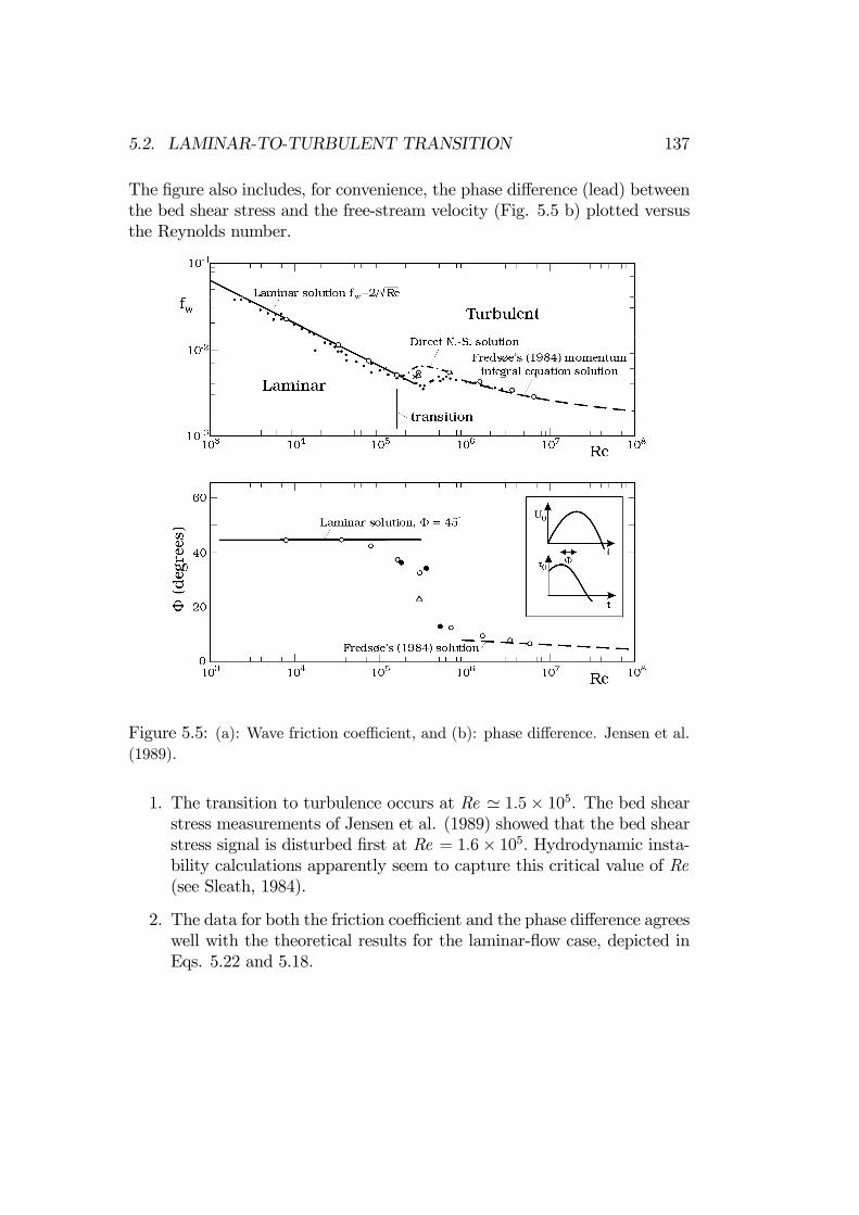
5.2. LAMINAR-TO-TURBULENT TRANSITION 137
The figure also includes, for convenience, the phase difference (lead) betweenthe bed shear stress and the free-stream velocity (Fig. 5.5 b) plotted versusthe Reynolds number.
Figure 5.5: (a): Wave friction coefficient, and (b): phase difference. Jensen et al.(1989).
1. The transition to turbulence occurs at Re 1.5× 10⁵. The bed shearstress measurements of Jensen et al. (1989) showed that the bed shearstress signal is disturbed first at Re = 1.6× 10⁵. Hydrodynamic insta-bility calculations apparently seem to capture this critical value of Re(see Sleath, 1984).
2. The data for both the friction coefficient and the phase difference agreeswell with the theoretical results for the laminar-flow case, depicted inEqs. 5.22 and 5.18.
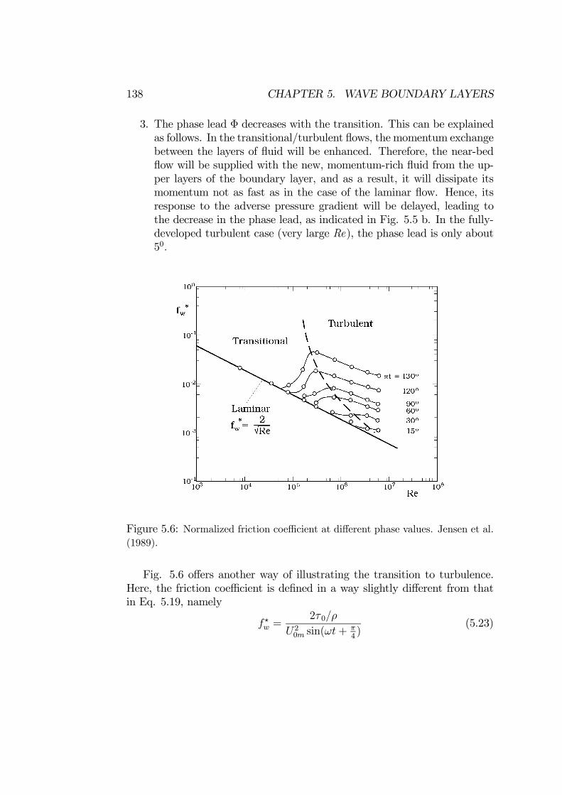
138 CHAPTER 5. WAVE BOUNDARY LAYERS
3. The phase lead Φ decreases with the transition. This can be explainedas follows. In the transitional/turbulent flows, the momentum exchangebetween the layers of fluid will be enhanced. Therefore, the near-bedflow will be supplied with the new, momentum-rich fluid from the up-per layers of the boundary layer, and as a result, it will dissipate itsmomentum not as fast as in the case of the laminar flow. Hence, itsresponse to the adverse pressure gradient will be delayed, leading tothe decrease in the phase lead, as indicated in Fig. 5.5 b. In the fully-developed turbulent case (very large Re), the phase lead is only about50.
Figure 5.6: Normalized friction coefficient at different phase values. Jensen et al.(1989).
Fig. 5.6 offers another way of illustrating the transition to turbulence.Here, the friction coefficient is defined in a way slightly different from thatin Eq. 5.19, namely
fw =2τ 0/ρ
U20m sin(ωt+π4)
(5.23)
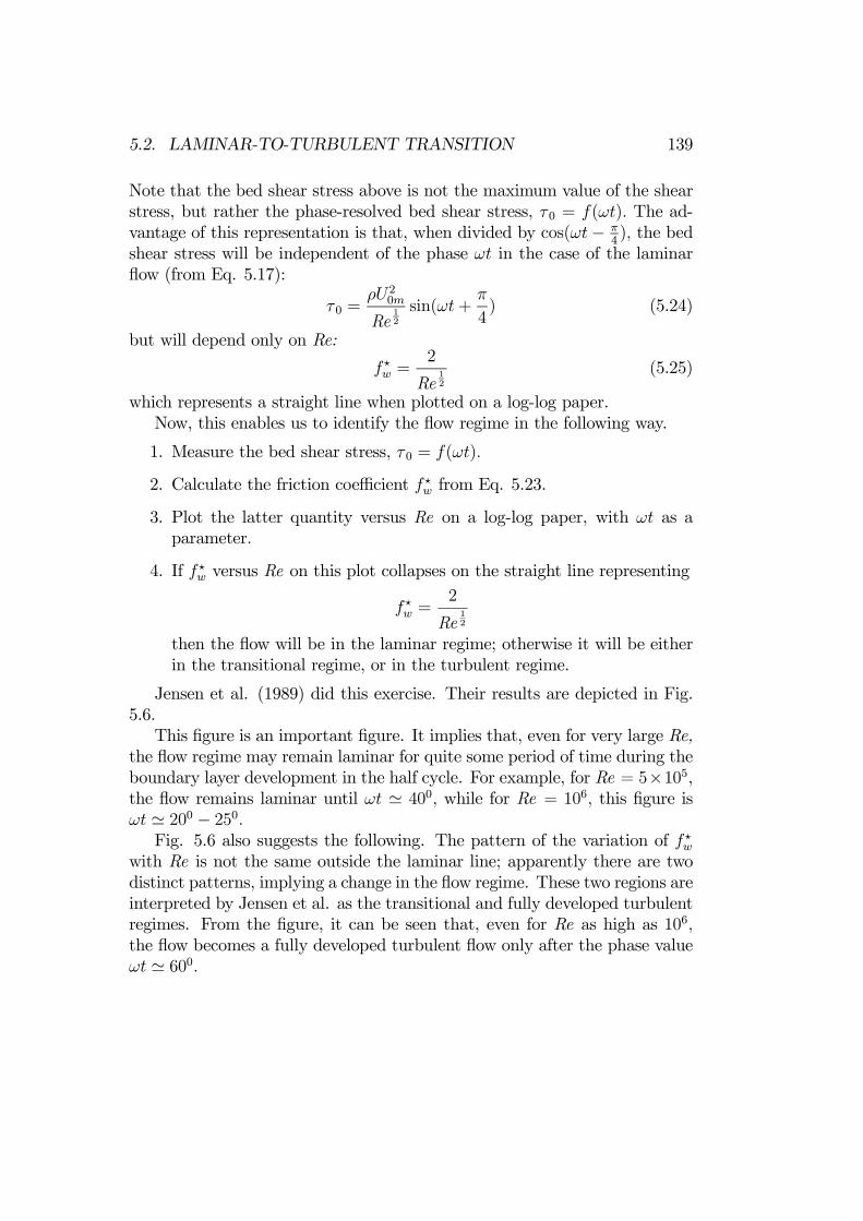
5.2. LAMINAR-TO-TURBULENT TRANSITION 139
Note that the bed shear stress above is not the maximum value of the shearstress, but rather the phase-resolved bed shear stress, τ 0 = f(ωt). The ad-vantage of this representation is that, when divided by cos(ωt− π
4), the bed
shear stress will be independent of the phase ωt in the case of the laminarflow (from Eq. 5.17):
τ 0 =ρU20m
Re12
sin(ωt+π
4) (5.24)
but will depend only on Re:
fw =2
Re12
(5.25)
which represents a straight line when plotted on a log-log paper.Now, this enables us to identify the flow regime in the following way.
1. Measure the bed shear stress, τ 0 = f(ωt).
2. Calculate the friction coefficient fw from Eq. 5.23.
3. Plot the latter quantity versus Re on a log-log paper, with ωt as aparameter.
4. If fw versus Re on this plot collapses on the straight line representing
fw =2
Re12
then the flow will be in the laminar regime; otherwise it will be eitherin the transitional regime, or in the turbulent regime.
Jensen et al. (1989) did this exercise. Their results are depicted in Fig.5.6.This figure is an important figure. It implies that, even for very large Re,
the flow regime may remain laminar for quite some period of time during theboundary layer development in the half cycle. For example, for Re = 5×10⁵,the flow remains laminar until ωt 400, while for Re = 106, this figure isωt 200 − 250.Fig. 5.6 also suggests the following. The pattern of the variation of fw
with Re is not the same outside the laminar line; apparently there are twodistinct patterns, implying a change in the flow regime. These two regions areinterpreted by Jensen et al. as the transitional and fully developed turbulentregimes. From the figure, it can be seen that, even for Re as high as 106,the flow becomes a fully developed turbulent flow only after the phase valueωt 600.

140 CHAPTER 5. WAVE BOUNDARY LAYERS
Figure 5.7: Sample velocity records. Re = 6× 10⁶. U0 was measured at y = 140mm, and u and v at y = 1 mm. Jensen et al. (1989).
5.3 Turbulent wave boundary layers
5.3.1 Ensemble averaging
Fig. 5.7 displays time series of the horizontal and vertical velocity compo-nents of the velocity in the boundary layer (the bottom two time series). Thetop time series is the free-stream velocity. This is from an experiment withRe = 6× 10⁶.The so-called ensemble averaging is used to calculate the mean values:
u(y,ωt) =1
N
N
j=1
u[y, ω(t+ (j − 1)T )] (5.26)
Likewise, for example, the root-mean-square (r.m.s.) value of the fluctuating

5.3. TURBULENT WAVE BOUNDARY LAYERS 141
Figure 5.8: Mean velocity distributions. Smooth bed. Re = 6×10⁶. Jensen et al.(1989).
velocity u = u− u,
u 2(y,ωt) =1
N − 1
N
j=1
[u[y, ω(t+ (j − 1)T )]− u(y,ωt)]212
(5.27)
5.3.2 Mean flow velocity
Fig. 5.8 shows the time development of the velocity profiles for Re = 6×10⁶.The way in which the velocity profiles evolve with time is similar to that inthe case of the laminar wave boundary layer (Fig. 5.3). Features such as theearly reversal of the flow near the bed, and the overshooting in the velocityprofiles are observed here, too.The velocity profiles in the previous figure are plotted in wall units on
semi-logarithmic plots in Fig. 5.9. The figure also includes the van Driestprofile (Eq. 2.97, the velocity profile obtained for steady boundary layers) asa reference line in each panel. Note that Uf used in the normalized quantitiesy+ =
yUfνand u
Ufis the temporal value (the phase resolved value) of the
friction velocity. Recall that the van Driest profile tends to the logarithmic
142 CHAPTER 5. WAVE BOUNDARY LAYERS
Figure 5.9: Mean velocity distributions in semi-log plot. Smooth bed. Re =6 × 10⁶. Solid curve: van Driest profile. Dashed lines: log law. Jensen et al.(1989).
distribution for large values of y+ (Eqs. 2.97 and 2.99)
u = Uf (A ln y+ +B) (5.28)
Fig. 5.9 shows the following.
1. The oscillatory-flow velocity distributions agree remarkably well withthe steady-flow ones in the range of ωt = 700 − 1100 where the flowexperiences almost zero pressure gradient.
2. The logarithmic layer exists already at ωt = 150 and is maintainedthroughout the ωt range from ωt 150 up to almost 1600.
3. At earlier phases, the logarithmic layer does not exist, however. Thisis because the boundary layer at these stages is not thick enough tohouse the logarithmic layer in it.
4. It may be noted that the velocity profiles in the early phases of theacceleration stage (where the pressure gradient is favourable) resem-ble quite closely those obtained in favourable pressure-gradient steadyboundary layers, and likewise, those in the later phases of the decel-eration stage (where the pressure gradient is adverse) resemble, again,quite closely the velocity distributions obtained in adverse pressure-gradient steady boundary layers (Coles, 1956).

5.3. TURBULENT WAVE BOUNDARY LAYERS 143
Figure 5.10: Mean velocity distributions. Sumer et al. (1987).
Figure 5.11: Shear stress distributions, corresponding to the velocity distributionsin the previous figure. Sumer et al. (1987).
Finally, note the following. Fig. 5.10 shows the semi-log plots of thevelocity distributions obtained in another research (Sumer et al., 1987), whileFig. 5.11 shows the corresponding shear stress distributions. As seen fromFig. 5.11, the constant stress layer is displaced to higher elevations in thelater phases (starting from ωt = 9π
12) of the deceleration stage. This means
that the logarithmic layer should also be displaced to these higher elevations.The velocity distributions may still be represented by the logarithmic law.However, Uf in such a representation cannot be the wall shear velocity, buta velocity defined by ( τ
ρ)12 where τ is the shear stress occurring at these
elevations rather than at the wall.

144 CHAPTER 5. WAVE BOUNDARY LAYERS
5.3.3 Flow resistance
The friction coefficient, defined by Eq. 5.19 or Eq. 5.20, has been deter-mined from experiments in oscillatory flows and plotted in Fig. 5.5 for bothtransitional and fully developed turbulent oscillatory boundary layers.The variation of the friction coefficient with Re in Fig. 5.5 in the fully
developed turbulent regime (Re 106) can be approximated by (Fredsøeand Deigaard, 1992, p. 29)
fw =0.035
Re0.16(5.29)
5.3.4 Turbulence quantities
Fig. 5.12 and 5.13 presents the turbulence data in terms of
u 2
Uf,
v 2
Uf,
w 2
Uf,−u vU2f
(5.30)
versus y+. Also plotted in the figures are the corresponding steady boundary-layer distributions (see, for example, Fig. 2.7).Except at very early phases of the acceleration stage, and also late phases
of the deceleration stage, the oscillatory-flow profiles appear to be in rea-sonable accord with the steady boundary-layer distributions throughout thephase space. See Jensen et al. (1989) for further details.
5.3.5 Effect of Reynolds number
Fig. 5.14 gives the mean velocity profiles for different Reynolds number.The characteristic features of the time development of the velocity profiles
shown in the preceding figure are as follows.
1. The velocity profile eventually reaches a state where the logarithmiclayer comes into existence.
2. This logarithmic layer grows in thickness, as one proceeds further inthe phase space ωt.
3. This continues to be the case until practically the point of reversal nearthe bed is reached.

5.3. TURBULENT WAVE BOUNDARY LAYERS 145
Figure 5.12: R.m.s. values of u , v and w . Smooth bed. Re = 6× 10⁶. Jensenet al. (1989).

146 CHAPTER 5. WAVE BOUNDARY LAYERS
Figure 5.13: Reynolds stresses. Smooth bed. Re = 6 ×10⁶. Jensen et al. (1989).
From the figure, it is seen that the higher Re, the earlier the logarithmiclayer comes into existence. This can be explained by reference to Fig. 5.6;From the latter figure, it is seen that, for the establishment of the logarithmiclayer, the flow has to reach the fully developed turbulent state.Jensen et al. (1989) also give the effect of Re on the turbulence quantities.
5.3.6 Boundary layer thickness
Fig. 5.15 presents the normalized boundary-layer thickness δaplotted against
Re. Here δ is the distance from the bed where the velocity becomes maximumat the phase value ωt = 900. The laminar flow solution has already been givenin Eq. 5.12; in terms of Re:
δ
a=3π
4(2
Re)12 (5.31)
From the figure, the boundary-layer thickness for storm conditions (verylarge Re)
δ
a= O(0.01) (5.32)
This corresponds to a boundary-layer thickness of δ = O(10 cm).

5.3. TURBULENT WAVE BOUNDARY LAYERS 147
Figure 5.14: Mean velocity distributions. Smooth bed. Diamonds: Re = 6×10⁶.Jensen et al. (1989). Empty circles: Re = 1.6× 10⁶. Filled circles: Re = 5× 10⁵.Dashed lines: Re = 5×10⁵, Spalart and Baldwin’s (1987) direct N.-S. simulation.Triangles: Re = 2.8× 10⁵, Hino et al. (1983). From Jensen et al. (1989).

148 CHAPTER 5. WAVE BOUNDARY LAYERS
Figure 5.15: Boundary-layer thickness. Smooth bed. Jensen et al. (1989).
Figure 5.16: Mean velocity u. Circles: Smooth bed. Triangles: Rough bed. Re= 6× 10⁶. Jensen et al. (1989).
5.3.7 Turbulent wave boundary layers over rough walls
Figs. 5.16-5.19 compare the rough-bed results with the corresponding smooth-bed ones in the tests of Jensen et al. (1989). Re = 6× 10⁶ and k+s = 84 inwhich k+s =
ksUfmν
where ks is Nikuradse’s equivalent sand roughness. Theparameter a
ks, on the other hand, is 3700.
From these figures, the following points appear to be noteworthy.
1. The description given in the preceding paragraphs of how the flow andturbulence evolve during one half-cycle is qualitatively the same for therough-bed flows, too.
2. The introduction of the roughness, however, results in a decrease in the

5.3. TURBULENT WAVE BOUNDARY LAYERS 149
Figure 5.17: R.m.s. value of u . Circles: Smooth bed. Triangles: Rough bed. Re= 6× 10⁶. Jensen et al. (1989).
Figure 5.18: R.m.s. value of v . Circles: Smooth bed. Triangles: Rough bed. Re= 6× 10⁶. Jensen et al. (1989).
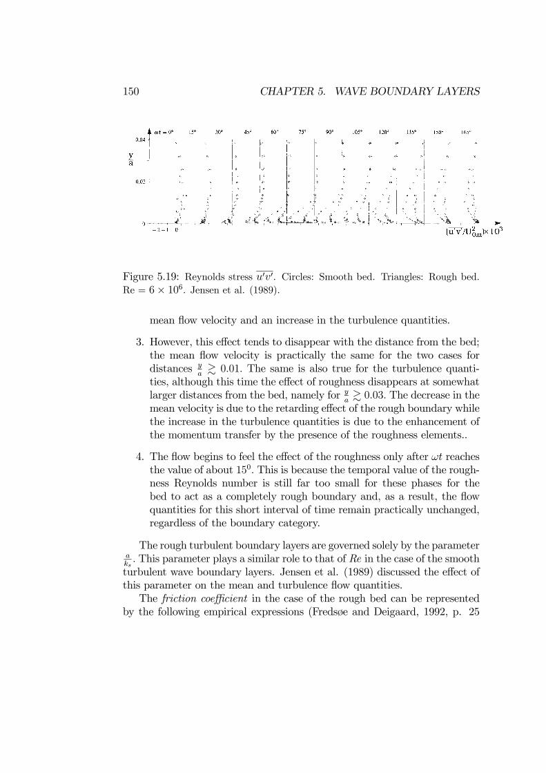
150 CHAPTER 5. WAVE BOUNDARY LAYERS
Figure 5.19: Reynolds stress u v . Circles: Smooth bed. Triangles: Rough bed.Re = 6× 10⁶. Jensen et al. (1989).
mean flow velocity and an increase in the turbulence quantities.
3. However, this effect tends to disappear with the distance from the bed;the mean flow velocity is practically the same for the two cases fordistances y
a0.01. The same is also true for the turbulence quanti-
ties, although this time the effect of roughness disappears at somewhatlarger distances from the bed, namely for y
a0.03. The decrease in the
mean velocity is due to the retarding effect of the rough boundary whilethe increase in the turbulence quantities is due to the enhancement ofthe momentum transfer by the presence of the roughness elements..
4. The flow begins to feel the effect of the roughness only after ωt reachesthe value of about 150. This is because the temporal value of the rough-ness Reynolds number is still far too small for these phases for thebed to act as a completely rough boundary and, as a result, the flowquantities for this short interval of time remain practically unchanged,regardless of the boundary category.
The rough turbulent boundary layers are governed solely by the parameteraks. This parameter plays a similar role to that of Re in the case of the smooth
turbulent wave boundary layers. Jensen et al. (1989) discussed the effect ofthis parameter on the mean and turbulence flow quantities.The friction coefficient in the case of the rough bed can be represented
by the following empirical expressions (Fredsøe and Deigaard, 1992, p. 25

5.4. OTHER ASPECTS 151
Figure 5.20: Boundary-layer thickness. Rough bed. Jensen et al. (1989).
and 26):fw = 0.04(
a
ks)−
14 when
a
ks> 50 (5.33)
fw = 0.4(a
ks)−
34 when
a
ks< 50 (5.34)
The latter expression is due to Kamphuis (1975) (Fredsøe and Deigaard,1992, p. 26).In the case of the transitional-category-bed wave boundary layers, the fric-
tion coefficient can be obtained from Kamphuis’ (1975) empirical diagrams.Also consult Fredsøe and Deigaard (1992, p. 33).Finally, Fig. 5.20 depicts the boundary-layer thickness. The figure shows
that, the boundary-layer thickness for storm conditions (very large aks)
δ
a= O(0.02) (5.35)
which corresponds to a boundary-layer thickness of δ = O(20 cm).
5.4 Other aspects
Several other aspects of wave boundary layers have been studied in recentyears. The following is a partial list of these studies undertaken at ISVA.Fredsøe, Sumer, Laursen and Pedersen (1993) have studied the non-
uniform wave boundary layers, where the non-uniformity is due to a suddenchange in the bed roughness, while Sumer, Laursen and Fredsøe (1993) have

152 CHAPTER 5. WAVE BOUNDARY LAYERS
studied the non-uniform wave boundary layers, where the non-uniformity isdue to the convergent/divergent geometry of the flow environment.Lodahl, Sumer and Fredsøe (1998) have investigated the combined os-
cillatory boundary layer and current in a circular pipe. The circular pipehas been selected in favour of a rectangular-section tunnel, to achieve a ”-clean” flow environment (to avoid secondary currents, and more importantlyto achieve a 2-D flow environment).Arnskov, Fredsøe and Sumer (1993) have studied combined wave and cur-
rent boundary-layer flow in a basin. In this study, the waves were propagatingat an angle to the current, including the normally incident waves.Tanaka, Sumer and Lodahl (1998) have studied the effect of cnoidal waves
on laminar wave boundary layers.Fredsøe, Andersen and Sumer (1999) have studied combined wave and
current boundary-layer flows over a ripple-covered bed.Fredsøe, Sumer, Kozakiewicz, Chua and Deigaard (2003) have studied
the effect of externally-generated turbulence on wave boundary layers.
5.5 References
1. Arnskov, M. M., Fredsøe, J. and Sumer, B. M. (1993): ”Bed shear stressmeasurements over a smooth bed in three-dimensional wave-currentmotion”. Coastal Engineering, Vol. 20, pp. 277- 316.
2. Coles, D. (1956): ”The law of the wake in a turbulent boundary layer”.J. Fluid Mech., vol. 1, p. 191.
3. Fredsøe, J. (1984): ”Turbulent boundary layer in wave-current mo-tion”. J. Hydraul. Eng. ASCE. 110, p. 1103.
4. Fredsøe, J., Andersen, K. H. and Sumer, B. M. (1999): ”Wave pluscurrent over ripple-covered bed”, Coastal Engineering, vol. 38, 177-221.
5. Fredsøe, J. and Deigaard, R. (1992). Mechanic of Coastal SedimentTransport. Advanced Series on Ocean Engineering., Vol. 3, WorldScientific.

5.5. REFERENCES 153
6. Fredsøe, J., Sumer, B.M., Laursen, T. S.and Pedersen, C. (1993): ”Ex-perimental investigations of wave boundary layers with a sudden changein roughness”. Journal of Fluid Mechanics, Vol. 252, pp.117-145.
7. Fredsøe, J., Sumer, B.M., Kozakkiewicz, A., Chua, L. H. C. and Deigaard,R. (2003): ”Effect of externally generated turbulence on wave boundarylayer”. Coastal Engineering, vol. 49, pp. 155-183.
8. Jensen, B. L., Sumer, B. M. and Fredsøe, J.: ”Turbulent oscillatoryboundary layers at high Reynolds numbers”. Journal of Fluid Mechan-ics, Vol. 206, p. 265, 1989.
9. Kamphuis, J. W. (1975): ”Friction factor under oscillatory waves”.J. Waterways, Port, Coastal and Ocean Eng. Div., ASCE, Vol. 101(WW2), pp. 135-144.
10. Lodahl, C. R., Sumer, B. M. and Fredsøe, J. (1998): ”Turbulent com-bined oscillatory flow and current in a pipe”, J. Fluid Mech., vol. 373,313-348.
11. Sleath, J. F. A. (1984): Sea Bed Mechanics, John Wiley & Sons.
12. Sumer, B. M., Jensen, B. L. and Fredsøe, J: ”Turbulence in oscilla-tory boundary layers”. Advances in Turbulence. Proc. 1st EuropeanConference, Lyon, France, published by Springer, p. 556, 1987.
13. Sumer, B. M., Laursen, T. S. and Fredsøe, J. (1993): ”Wave boundarylayers in a convergent tunnel”. Coastal Engineering, Vol. 20, pp. 317-342.
14. Tanaka, H., Sumer, B. M. and Lodahl, C. (1998): ”Theoretical andexperimental investigation on laminar boundary layers under cnoidalwave motion”, Coastal Engineering Journal, vol. 40, No. 1, 81-98.

154 CHAPTER 5. WAVE BOUNDARY LAYERS

Chapter 6
Turbulence modelling
6.1 The closure problem
We have derived the basic equations of turbulent flows in Chapter 1. Theseequations are the continuity equation (Eq. 1.6) and the Reynolds equations(the equations of motion) (Eq. 1.14), respectively:
∂ui∂xi
= 0 (6.1)
ρ(∂ui∂t+ uj
∂ui∂xj
) = ρgi +∂
∂xj(σij − ρuiuj) (6.2)
with the quantity σij, the stress on the fluid
σij = −pδij + μ(∂ui∂xj
+∂uj∂xi
) (6.3)
and the Reynolds stress tensor
−ρuiuj =
⎡⎣ −ρu1u1 − ρu1u2 − ρu1u3−ρu2u1 − ρu2u2 − ρu2u3−ρu3u1 − ρu3u2 − ρu3u3
⎤⎦ (6.4)
in which there are, due to symmetry, six independent Reynolds stresses (threediagonal components and three off-diagonal ones).As has already been discussed (Chapter 1), there are four equations for
the mean flow, i.e., the continuity equation (Eq. 1.6) and the three Reynolds
155

156 CHAPTER 6. TURBULENCE MODELLING
equations (Eq. 1.14) whereas there are ten unknowns (namely, three com-ponents of the velocity, ui, and the pressure, p, and six components of theReynolds stress, −ρuiuj), hence the system is not closed. This problem isknown as the closure problem of turbulence.To close the system, we must find enough number of equations to solve
for the unknowns. We do this through turbulence modelling.(In the case of laminar flow, there are four unknowns (namely, three
components of the velocity, ui, and the pressure, p), and four equations, i.e.,the continuity equation (Eq. 1.4) and three N.-S. equation (Eqs. 1.8 and1.9). Therefore, the system is closed.)
6.2 Turbulence models
There are several kinds of turbulence models the most important of whichare
1. Algebraic models;
2. Turbulence-energy equation models; and
3. Simulation models such as Direct Numerical Simulation (DNS), LargeEddy Simulation (LES) and Detached Eddy Simulation (DES).
Algebraic models, also known as the zero-equation models, are the sim-plest of all turbulent models. Here, (1) the Reynolds stress is expressed asthe product of a turbulence viscosity (eddy viscosity) and the mean strainrate, the so-called Boussinesq eddy-viscosity approximation, and (2) the tur-bulence viscosity, in turn, is often computed in terms of a mixing length. Ofthe algebraic models, the mixing-length model is the simplest and the most”popular” one. This model will be described in the next section.Turbulence-energy equation models are advanced models. Here, too, the
Reynolds stress is expressed as the product of a turbulence viscosity (eddyviscosity) and the mean strain rate. However, the turbulence viscosity is notcomputed in terms of a mixing length, but rather in terms of the turbulencekinetic energy, k = 1
2(uiui). There are two kinds of turbulence-energy equa-
tion models: (1) One-equation models, and (2) Two-equations models. As anexample, the so-called k−ω model, a two-equations model, will be describedin the following paragraphs.

6.3. MIXING-LENGTH MODEL 157
Simulation models are most advanced models. These models directly ad-dress the turbulence process itself, and therefore they do not involve the aforementioned closure problem. In a DNS study, a complete time-dependent so-lution of the Navier-Stokes equations and the continuity equation is sought.Therefore the solution furnishes the time series of (1) the three componentsof the velocity and (2) the pressure in 3-D space. Up until now, only lowReynolds number-flows are calculated with the DNS method. For largeReynolds numbers, the scales of the dissipative part of turbulence motionare so small that this kind of small scale motion can not be resolved in anumerical calculation (the number of grid points required to resolve this mo-tion increases approximately with Re3, Rodi, 1992). However, the upperlimit of the Reynolds number range is pushed to higher and higher values asmore and more computer power becomes available. Rogallo and Moin (1984)gives a review of the DNS method where the principal/early publications arecited. Regarding the LES model, here the large eddies (large-scale motions)are computed while the smallest eddies are modelled. The details of the LESmodel along with an application example are given in the chapter.Wilcox’s (1994) book can be consulted for a detailed account of turbulence
models.
6.3 Mixing-length model
The mixing-length model is an algebraic model. We will describe this modelwith reference to the steady boundary-layer flow close to a smooth or roughwall (i.e., in the constant stress layer, see Section 2.1).
6.3.1 Turbulent transport of momentum
Under this subsection, we will focus on the turbulent transport of momentum.We need this piece of information to develop the mixing-length theory/model.The treatment will be quite general, not necessarily limited to the flow closeto a wall.For this, we refer to Fig. 6.1, and we consider a small fluid element (a
fluid parcel) adjacent to the unit area indicated in Fig. 6.1, A (Fig. 6.2),at time t. This fluid parcel will be transported to the other side of the areaduring the time interval ∆t (B, Fig. 6.2), and this is due to the turbulentmotion. (No such transportation would occur if the flow was in the laminar
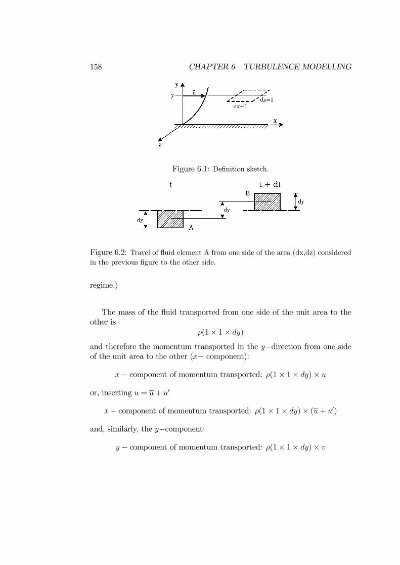
158 CHAPTER 6. TURBULENCE MODELLING
Figure 6.1: Definition sketch.
Figure 6.2: Travel of fluid element A from one side of the area (dx,dz) consideredin the previous figure to the other side.
regime.)
The mass of the fluid transported from one side of the unit area to theother is
ρ(1× 1× dy)
and therefore the momentum transported in the y−direction from one sideof the unit area to the other (x− component):
x− component of momentum transported: ρ(1× 1× dy)× u
or, inserting u = u+ u
x− component of momentum transported: ρ(1× 1× dy)× (u+ u )
and, similarly, the y−component:
y − component of momentum transported: ρ(1× 1× dy)× v

6.3. MIXING-LENGTH MODEL 159
Now, Newton’s second law (for the x−direction)
Fx =d
dt[x− component of momentum transported]
=d
dt[ρ(1× 1× dy)× (u+ u )]
= ρd(dy)
dt(u+ u )
in which Fx is the force generated by this momentum transport. Here,d(dy)dt
=ddt(Vertical distance travelled by fluid) = v = v , and therefore
Fx = ρv (u+ u )
and by time averaging
Fx = ρv (u+ u ) = ρv u+ ρu v ) = 0 + ρu v = ρu v (6.5)
Likewise, Newton’s second law for the y−direction gives
Fy = ρv v (6.6)
These forces, Fx and Fy, are exerted on the unit area indicated in Fig. 6.1,and therefore they are, respectively, the shear and normal stresses. (Noticethat these stresses are induced by turbulence (Fig. 6.3.) So the aboveanalysis demonstrates that
1. The turbulent transport of momentum in the y−direction generatesstresses in the fluid;
Figure 6.3: Forces (stresses) induced by turbulence.
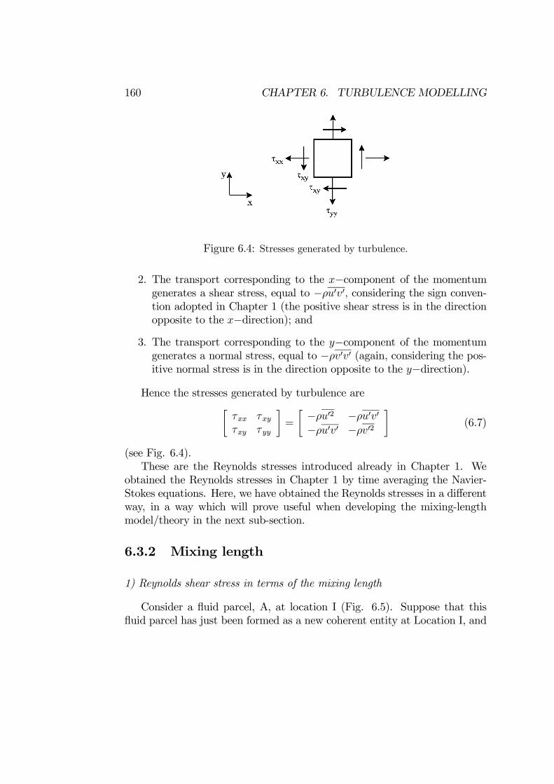
160 CHAPTER 6. TURBULENCE MODELLING
Figure 6.4: Stresses generated by turbulence.
2. The transport corresponding to the x−component of the momentumgenerates a shear stress, equal to −ρu v , considering the sign conven-tion adopted in Chapter 1 (the positive shear stress is in the directionopposite to the x−direction); and
3. The transport corresponding to the y−component of the momentumgenerates a normal stress, equal to −ρv v (again, considering the pos-itive normal stress is in the direction opposite to the y−direction).
Hence the stresses generated by turbulence are
τxx τxyτxy τ yy
=−ρu 2 −ρu v−ρu v −ρv 2 (6.7)
(see Fig. 6.4).These are the Reynolds stresses introduced already in Chapter 1. We
obtained the Reynolds stresses in Chapter 1 by time averaging the Navier-Stokes equations. Here, we have obtained the Reynolds stresses in a differentway, in a way which will prove useful when developing the mixing-lengthmodel/theory in the next sub-section.
6.3.2 Mixing length
1) Reynolds shear stress in terms of the mixing length
Consider a fluid parcel, A, at location I (Fig. 6.5). Suppose that thisfluid parcel has just been formed as a new coherent entity at Location I, and
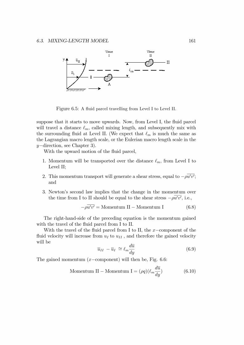
6.3. MIXING-LENGTH MODEL 161
Figure 6.5: A fluid parcel travelling from Level I to Level II.
suppose that it starts to move upwards. Now, from Level I, the fluid parcelwill travel a distance m, called mixing length, and subsequently mix withthe surrounding fluid at Level II. (We expect that m is much the same asthe Lagrangian macro length scale, or the Eulerian macro length scale in they−direction, see Chapter 3).With the upward motion of the fluid parcel,
1. Momentum will be transported over the distance m, from Level I toLevel II;
2. This momentum transport will generate a shear stress, equal to −ρu v ;and
3. Newton’s second law implies that the change in the momentum overthe time from I to II should be equal to the shear stress −ρu v , i.e.,
−ρu v =Momentum II−Momentum I (6.8)
The right-hand-side of the preceding equation is the momentum gainedwith the travel of the fluid parcel from I to II.With the travel of the fluid parcel from I to II, the x−component of the
fluid velocity will increase from uI to uII , and therefore the gained velocitywill be
uII − uI ∼= mdu
dy(6.9)
The gained momentum (x−component) will then be, Fig. 6.6:
Momentum II−Momentum I = (ρq)( mdu
dy) (6.10)

162 CHAPTER 6. TURBULENCE MODELLING
Figure 6.6: Volume associated with Fluid Parcel A passing through per unit area.
in which q is the volume associated with the fluid parcel (Fig. 6.5) passingthrough per unit area per unit time (Fig. 6.6). The quantity q is
q = Vt(1× 1) = Vt
and therefore the gained momentum (x−component) will be
Momentum II−Momentum I = ρVt mdu
dy(6.11)
in which Vt is the fluid velocity in the vertical direction, an average velocityrepresenting the vertical velocity of the fluid parcel over the travelled distancem. From Eqs. 6.8 and 6.11:
−ρu v =Momentum II−Momentum I = (6.12)
= ρVt mdu
dy(6.13)
2) Boussinesq eddy-viscosity approximation and Prandtl’s mixing lengthhypothesis
Now, drawing an analogy to Newton’s friction law
τ = μdu
dy(6.14)

6.3. MIXING-LENGTH MODEL 163
the turbulence shear stress can be written as (as was first suggested by Boussi-nesq in 1877)
−ρu v = μtdu
dy(6.15)
in which μt is called turbulence viscosity (or eddy viscosity). Hence, fromEqs. 6.13 and 6.15, the turbulence viscosity is
μt = ρ mVt (6.16)
The hypothesis leading to Eq. 6.16 is known as Prandtl’s mixing-lengthhypothesis.(It may be noted that, in a recent publication, Nielsen and Teakle, 2004,
develop a theory of turbulent diffusion of momentum and suspended particles,a finite-mixing-length theory, in which the turbulence viscosity is expressedas μt = ρ mVt(1+O( m/L)
2). Here L is the scale of the velocity distributionu(y). It may also be noted that different diffusivities exhibited by different”species”, like density, heat and salinity, in turbulent flows may be qualita-tively explained in terms of Nielsen and Teakle’s theory. See also Absi, 2005,in relation to the latter publication.)To sum up at this point: (1) The Reynolds shear stress is expressed as the
product of a turbulence viscosity (eddy viscosity), μt, and the mean strainrate, du
dy(Eq. 6.15), the so-called Boussinesq eddy-viscosity approximation;
and (2) The turbulence (eddy) viscosity, in turn, is computed in terms of themixing length (Eq. 6.16).
3) Prandtl’s second hypothesis
The question is, however: What is Vt? To assess and therefore model this,we consider the control volume in Fig. 6.7. The motion associated with thefluid parcel A in Fig. 6.5 is from the left bottom corner of the control volumeto the right top corner, and involves three kinds of velocities:
1. The vertical velocity Vt at the instant I (It is important to notice thatthere is no vertical velocity at the instant II because the fluid parcelmixes with the surrounding fluid at II; Recall the definition of themixing length m.);
2. The horizontal velocity at the instant I; and

164 CHAPTER 6. TURBULENCE MODELLING
Figure 6.7: Control volume.
3. The horizontal velocity at the instant II.
The amount of fluid entering the control volume in the vertical direction(associated with this motion) per unit time is then:
Vt × dx (6.17)
while the amount of fluid entering the control volume in the horizontal di-rection per unit time at the instant I:
uI × m (6.18)
and that leaving the control volume in the horizontal direction per unit timeat the instant II:
uII × m (6.19)
Continuity requires:
Vt × dx+ uI × m = uII × m
and therefore
Vt = (uII − uI) m
dx
and since O( m) = O(dx) (small), then
Vt ∼= uII − uI
or from Eq. 6.9:
Vt ∼= mdu
dy

6.3. MIXING-LENGTH MODEL 165
We write the term dudyin terms of its absolute value to ensure that the amount
of fluid passing through the unit area, i.e., q(= v) is always positive (Fig.6.5):
Vt = mdu
dy(6.20)
This is known as Prandtl’s second hypothesis.With the latter hypothesis (Eq. 6.20), the turbulence (eddy) viscosity
from Eq. 6.16 is expressed as
μt = ρ 2m
du
dy(6.21)
4) van Driest mixing length
The fourth step is to determine the mixing length in the preceding equa-tion. Until now the analysis is given for the general case, and therefore it canbe implemented for any distance y from the wall. However, from now on,we will restrict our attention to the region close to the wall, the layer calledconstant stress layer. (See Chapter 2). So, y is so small that we are in theconstant stress layer, τ τ 0, and for this
y h
in which h is the flow depth in the case of an open channel flow, or it is theradius in the case of a pipe flow, or the boundary-layer thickness in the caseof a boundary layer over a wall. (See discussion in Section 2.1.2);On the other hand, y should be sufficiently large, so large that the trans-
port of momentum is due to turbulence. (Viscosity is neglected in the trans-port of momentum; This is for the case of the smooth wall. The rough-wallcase will be treated later.) We require that the transport of momentum isdue to turbulence because the previously described mixing length (Section1.3.2) is essentially based on the turbulent transport of momentum. Thislast condition requires that y+ should be
y+ > 30− 70
in which y+ = yUfν, Uf being the wall shear stress (friction) velocity (Chapter
2).

166 CHAPTER 6. TURBULENCE MODELLING
Now, we should expect that the mixing length (for y values in the rangey h and y+ > 30 − 70) increases with increasing distance from the wall,and the simplest form of this dependence is
m = κy (6.22)
in which κ is a constant. From the solution for the velocity (Eq. 6.28),κ turns out to be the von Karman constant (κ = 1
A= 0.4) introduced in
Chapter 2. Eq. 6.22 is valid for the ranges 30− 70 < y+, and y h.van Driest (1956) revised Eq. 6.22 so as to accommodate the influence of
viscosity in the transport of momentum. This led to
m = κy[1− exp(−y+
Ad)] (6.23)
in which Ad is called the damping coefficient, and taken as 25, and thisequation for the mixing length is valid for the range 0 ≤ y h. From Eq.6.23, it is seen that
m → κy, for large values of y+ (6.24)
while
m → 0, as y+ → 0 (6.25)
The latter implies that there will be no turbulent transport of momentumas the wall is approached. Note that, for rough-wall flows, the mixing-lengthwill inevitably change. We shall consider the transitional and rough-wallsituations later.
5) Summary of the model equations and solution
Eqs. 6.15, 6.21 and 6.23 are the model equations:
−ρu v = μtdu
dy
μt = ρ 2m
du
dy
m = κy[1− exp(−y+
Ad)]
6.3. MIXING-LENGTH MODEL 167
So, for the problem we consider, i.e., the steady boundary-layer flow closeto a smooth wall (in the constant stress layer, see Section 2.1), there are threemodel equations (the preceding equations), and one Reynolds equation, Eq.2.87, i.e., altogether four equations, and four unknowns, namely, u, −ρu v ,μt, and m. Hence, the system is closed. Therefore the unknowns can bedetermined. Of particular interest is the velocity, u. The solution for thelatter quantity is obtained in Section 2.3.1 (Eq. 2.97):
u = 2Ufy+
0
dy+
1 + 1 + 4κ2y+2[1− exp(−y+
Ad)]2
1/2(6.26)
(the van Driest velocity distribution, Fig. 2.20). This equation is valid inthe constant stress layer, namely for the range 0 ≤ y h.)For small values of y+, the van Driest profile reduces to the linear velocity
distribution in the viscous sublayer (Eq. 2.20),
u
Uf= y+ (6.27)
while, for large values of y+, it reduces to the logarithmic velocity distributionin the logarithmic layer (Eq. 2.20),
u = Uf (A ln y+ +B) (6.28)
It is seen from Fig. 2.20 that the van Driest profile agrees remarkably wellwith the experiment.
6) Mixing length in the case of transitional and rough walls and solution
In this case, the mixing length may be given as (Cebeci and Chang, 1978)
m = κ(y +∆y)[1− exp(−(y+ +∆y+)
Ad)] (6.29)
y in the above equation is measured from the level where the velocity u iszero. This level lies almost at the top of the roughness elements, as discussedin Section 2.3.1 (y here should not be confused with the distance measuredfrom the theoretical wall. y+∆y is the distance measured from the theoreticalwall. See the detailed discussion in Section 2.3.1).

168 CHAPTER 6. TURBULENCE MODELLING
∆y is the so-called coordinate displacement, or the coordinate shift (seeExample 5 in Section 2.3.1), and given by Cebeci and Chang (1978)
∆y+ = 0.9[ k+s − k+s exp(−k+s
6)]; 5 < k+s < 2000 (6.30)
in which k+s is the roughness Reynolds number (ks being Nikuradse’s equiv-alent sand roughness):
k+s =ksUfν
(6.31)
Here the distance from the wall y should be in the interval 0 ≤ y h wherethe upper boundary ensures that the y levels lie in the constant stress layer.The solution for u for the set of the model equations along with the
Reynolds equation is obtained in Section 2.3.1 (Eq. 2.103):
u = 2Ufy+
0
dy+
1 + 1 + 4κ2(y+ +∆y+)2[1− exp(− (y++∆y+)Ad
)]21/2
(6.32)
Fig. 2.21 displays the velocity profiles obtained from the preceding equationincluding the smooth-wall profile. In Fig. 2.21, a represents the linear profilein the viscous sublayer (Eq. 6.27), b the logarithmic profile (Eq. 6.28) in thecase of the hydraulically smooth wall, and c the logarithmic profile in thecase of the completely rough wall (Eq. 2.65), namely, by putting z = y+∆y,
u = AUf ln(30z
ks) (6.33)
z being measured from the theoretical wall.
7) Turbulence quantities
The turbulence quantities, namely the Reynolds stresses, −ρu 2, −ρv 2,−ρw 2 and−ρu v , also are unknowns. The Reynolds shear stress, −ρu v , canbe determined, using the model equation−ρu v = μt
dudy, once the velocity u is
computed. The mixing-length model is ”designed” only to be able to handlethe velocity u, (and from the latter, the Reynolds stress −ρu v ). It does notoffer solutions for the other three unknowns, the turbulence quantities −ρu 2,−ρv 2 and −ρw 2.

6.4. K-OMEGA MODEL 169
6.4 k-omega model
This model is a turbulence-energy equation model. As mentioned in the pre-ceding paragraphs, there are two kinds of turbulence-energy equation model,one-equation model and two-equations model. The k − ω model is a two-equations model.There are three versions of the k−ω model in the literature: (1) the origi-
nal k−ω model, which is due to Wilcox (1994), (2) the k−ω, BSL (baseline)model, and (3) the k−ω, SST (shear-stress transport) model. The latter twomodels were developed by Menter (1993) to improve Wilcox’s original modelso that an even higher sensitivity could be obtained for adverse-pressure-gradient flows. In this section, we will describe the k − ω, SST model.Incidentally, the following note is worth mentioning. Menter (1993) made
an extensive comparison between (1) the classic k− ε model; (2) the originalk − ω model; (3) the k − ω, BSL model; and (4) the k − ω, SST model forvarious well documented flows. The tested flows were, among others, twokinds of adverse pressure gradient flow (one having a very strong adversepressure gradient, so strong that separation occurs); the backward-facing-step flow; and the flow past a NACA 4412 airfoil at an angle of attack nearmaximum lift condition. The latter two flows also have substantial adversepressure gradient effects. The main conclusion from this inter-comparisonexercise was that the k−ω, SST model gave the most accurate results whilethe k − ε model did not yield as accurate results as the other three for thetested adverse-pressure-gradient flow cases.
6.4.1 Model equations
There are two basic equations in the k − ω model: one equation for k, andthe other equation for ω in which k is the turbulent kinetic energy (Eq. 1.31or Eq. 6.36) and ω the specific dissipation of turbulent kinetic energy (Eq.6.37). (We will use the symbol k for turbulent energy in favour of Kt, to beconsistent with the usual notation used in the literature in conjunction withturbulence modelling.)The equation for k:
∂ρk
∂t+
∂ρujk
∂xj− ∂
∂xj(μ+ σkμt)
∂k
∂xj= τ ij
∂ui∂xj− β∗ρkω (6.34)
(It should be noted that this equation is in a form slightly different from that
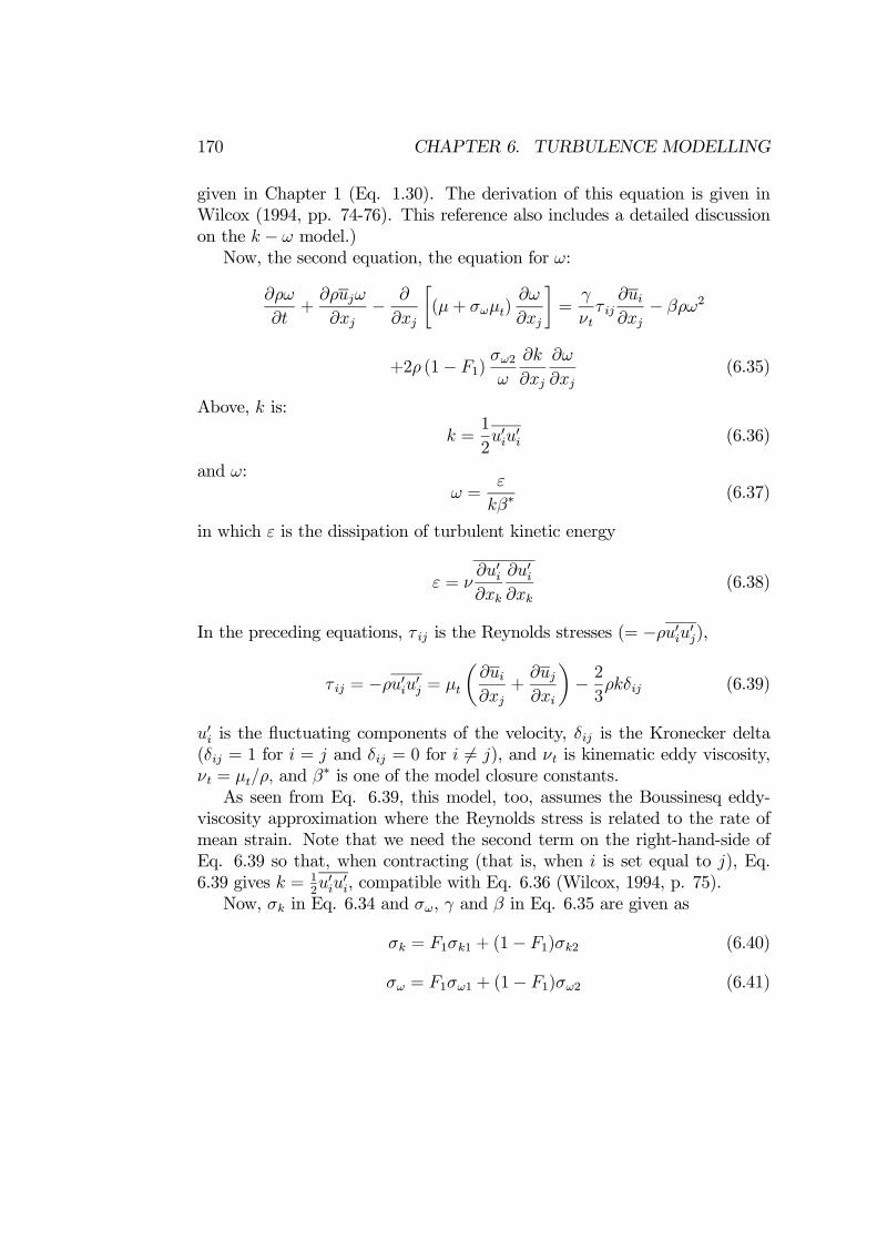
170 CHAPTER 6. TURBULENCE MODELLING
given in Chapter 1 (Eq. 1.30). The derivation of this equation is given inWilcox (1994, pp. 74-76). This reference also includes a detailed discussionon the k − ω model.)Now, the second equation, the equation for ω:
∂ρω
∂t+
∂ρujω
∂xj− ∂
∂xj(μ+ σωμt)
∂ω
∂xj=
γ
νtτ ij
∂ui∂xj− βρω2
+2ρ (1− F1)σω2
ω
∂k
∂xj
∂ω
∂xj(6.35)
Above, k is:
k =1
2uiui (6.36)
and ω:ω =
ε
kβ∗(6.37)
in which ε is the dissipation of turbulent kinetic energy
ε = ν∂ui∂xk
∂ui∂xk
(6.38)
In the preceding equations, τ ij is the Reynolds stresses (= −ρuiuj),
τ ij = −ρuiuj = μt∂ui∂xj
+∂uj∂xi
− 23ρkδij (6.39)
ui is the fluctuating components of the velocity, δij is the Kronecker delta(δij = 1 for i = j and δij = 0 for i = j), and νt is kinematic eddy viscosity,νt = μt/ρ, and β∗ is one of the model closure constants.As seen from Eq. 6.39, this model, too, assumes the Boussinesq eddy-
viscosity approximation where the Reynolds stress is related to the rate ofmean strain. Note that we need the second term on the right-hand-side ofEq. 6.39 so that, when contracting (that is, when i is set equal to j), Eq.6.39 gives k = 1
2uiui, compatible with Eq. 6.36 (Wilcox, 1994, p. 75).
Now, σk in Eq. 6.34 and σω, γ and β in Eq. 6.35 are given as
σk = F1σk1 + (1− F1)σk2 (6.40)
σω = F1σω1 + (1− F1)σω2 (6.41)

6.4. K-OMEGA MODEL 171
γ = F1γ1 + (1− F1)γ2 (6.42)
β = F1β1 + (1− F1)β2 (6.43)
in which σk1, σk2, σω1, σω2, γ1, γ2, β1 and β2, the model constants, arecombined as a function of the distance z to the nearest wall with the so-called blending function , F1.
6.4.2 Model constants
The model constants for inner (wall) region are:β1 β∗ γ1(=
β1β∗ −
σω1κ2√β∗) σk1 σω1
0.0750 0.09 0.567 0.85 0.5
and for the outer region (κ in the tables is the von Karman constant):β2 β∗ γ2(=
β2β∗ −
σω2κ2√β∗) σk2 σω2
0.0828 0.09 0.463 1.0 0.856
6.4.3 Blending function F1
The blending function F1 is
F1 = tanh arg41 (6.44)
and
arg1 = min max
√k
0.09ωz;500ν
z2ω;4ρkσω2
(CDkω)z2(6.45)
with
(CDkω) = max 2ρσω2
ω
∂k
∂xj
∂ω
∂xj; 10−20 (6.46)

172 CHAPTER 6. TURBULENCE MODELLING
Figure 6.8: Computation domain.
6.4.4 Eddy viscosity and Blending function F2In the k − ω, SST model, the eddy viscosity is calculated from
μt = ρ0.3k
max (0.3ω;ΩF2)(6.47)
where Ω is the absolute value of the vorticity. The function F2 in Eq. 6.47is another blending function, defined by
F2 = tanh arg22 (6.48)
in which
arg2 = max 2
√k
0.09ωz;500ν
z2ω(6.49)
Both F1 and F2 take the value unity at the wall and gradually decrease andapproach to zero as the distance from the wall is increased.
6.4.5 Boundary conditions
The boundaries of the computational domain (Fig. 6.8) are (1) Inlet, (2)Outlet, (3) Symmetry Boundaries and (4) Walls (e.g., the bed in the example

6.4. K-OMEGA MODEL 173
given in Fig. 6.8 and the surface of a rigid body present in the computationaldomain, if any).
1) Inlet and outlet boundary conditions
At the inlet, zero transverse, and vertical velocities are specified. Atthe outlet, zero-gradient conditions (∂/∂n = 0), Neumann conditions, areapplied for all quantities.
2) Symmetry boundaries
At the symmetry boundaries , Neumann conditions are applied for k andω and for the three components of the velocity (u, v and w). This is (1) atthe sides and (2) at the top surface of the computational domain where a”lid” is placed in the case when the model cannot handle the free surface,Fig. 6.8).
3) Walls (e.g., the bed and/or the surface of a rigid body)
1. Zero velocity is specified for u , v and w.2. Zero turbulent energy is specified for k when the wall is smooth, while
the Neumann condition is applied when the wall is rough and transitional.Regarding the latter condition, experiments reveal that the Neumann condi-tion is satisfied (∂k/∂n = 0) at the wall for rough boundaries, n being thedirection normal to the wall (Nezu, 1977, Sumer et al., 2001 and 2003). Avalidation exercise for the case of a steady boundary layer in an open chan-nel flow revealed a much better agreement with the experiments (Nezu, 1977,and Sumer et al., 2001) when the boundary condition was taken in the formof the Neumann condition (Roulund, 2000, p. 25).3. The Dirichlet condition is applied for ω, namely
ω = SrU2fν
at the wall (6.50)
where Uf = τ o/ρ is the friction velocity based on the wall shear stress τ o.The quantity Sr is a tuning parameter, and it is used to account for the bedroughness:
Sr =
⎧⎨⎩ 40k+s
3
, k+s < 20.2100
(k+s )0.85 , k+s > 20.2
(6.51)

174 CHAPTER 6. TURBULENCE MODELLING
where k+s = (ksUf)/ν is the wall roughness in wall units, and ks is Nikuradse’sequivalent sand roughness. Wilcox (1994) was the first to introduce theboundary condition in Eq. 6.50. The tuning parameter Sr was given byWilcox (1994) as in Eq. 6.51, but with constants slightly different fromthose in Eq. 6.51 due to the special implementation of the velocity boundaryconditions. With the present constants (Eq. 6.51), the friction velocitydetermined for a wide range of velocities for the case of the undisturbed flowwas found to agree rather well with that obtained from the classic Colebrookand White equation (the difference being less than 6%, depending on thewall roughness, Roulund, 2000, p. 23).4. For the implementation of the preceding boundary condition, the wall
shear stress, τ 0(= ρU2f ), is needed. Traditionally, τ 0 is calculated from τ 0 =
(μ + μt)(∂ui∂xj
+∂uj∂xi)Wall. However, it may also be calculated from the van
Driest (1956) velocity profile (Eq. 6.32):
u
Uf= 2
y+
0
dy+
1 + 1 + 4κ2 (y+ +∆y+)2 1− exp −y++∆y+A
2(6.52)
This improves the stability of the model and allows a coarser mesh resolutionat the bed, as was revealed by the work of Roulund et al. (2005). In theimplementation of Eq. 6.52, u is taken as the tangential velocity in the celladjacent to the wall.Similar implementation of the bed shear stress in the wall boundary con-
ditions is reported in Sørensen (1995) for the k − ε model.As a final remark in conjunction with the previous description, it may be
emphasized that the k − ω model is a well tested model and has been usedsuccessfully in various contents in computational fluid dynamics (Wilcox,1994, Menter, 1993). The only change made in the present implementationis the values of the constants in Eq. 6.51 which are slightly different fromthose originally given by Wilcox (1994) (item 3 above), plus the way in whichthe wall shear stress is calculated is through the van Driest equation (item 4above).
6.4.6 Numerical computation
To sum up, the set of equations which needs to be solved consists of
1. The continuity equation, Eq. 6.1;

6.4. K-OMEGA MODEL 175
2. The Reynolds equations, Eqs. 6.2-6.4; and
3. The model equations, Eqs. 6.34-6.35.
With the solution, the three velocity components, the pressure, the tur-bulent kinetic energy and the specific dissipation of turbulent kinetic energyare calculated.Unlike the mixing-length model, this set of equations is too complex for
one to seek analytical solutions. Instead, the equations are solved numer-ically. To this end, one resorts to a CFD (Computational-Fluid-Dynamic)code coupled with a turbulence model (e.g., the k − ω model in the presentcase) which is incorporated into the code. CFD codes may also offer variousturbulence-modelling options. In these codes, the momentum, continuityand turbulence-model equations are typically transformed into curvilinearcoordinates, and they may be linearized and decoupled. The equations arediscretized, using a computational mesh (e.g., the latter can be based ona multi-block structure with each block containing N3 computational cellswhere N is the number of cells in each spatial direction.)The k − ω model was implemented in a Ph.D. study to calculate flow
around a vertical cylinder (a bridge pier or a pile) in relation to numericalmodelling of scour around such structures (Roulund, 2000, and Roulund etal., 2005). More information about the model, boundary conditions, numer-ical computation, etc. with regard to the previously mentioned applicationcan be found in the latter publications.
6.4.7 An application example
Under this subsection, we will present the results of a small study where thek − ω model was employed.The CFD code used in this study, EllipSys3D, is a three-dimensional
general purpose flow solver (an incompressible general purpose Navier-Stokessolver). It is a multiblock finite-volume numerical model that solves theincompressible Reynolds equations (Eqs. 6.2-6.2). The k − ω, SST model isused as the turbulence closure. EllipSys3D has been developed at the RisøNational Laboratory, Denmark and at the Technical University of Denmark,Department of Fluid Mechanics. The code offers a variety of turbulence-model options, including the k − ω, SST model. The basic principles of themodel are described in Michelsen (1992) and Sørensen (1995).

176 CHAPTER 6. TURBULENCE MODELLING
The problem studied in this example is a steady boundary layer flow in anopen channel with a smooth, or alternatively, a rough bed. The flow domainis the same as that depicted in Fig. 6.8. As the model does not have thefree-surface facility, a lid is placed at the top surface of the computationaldomain. The boundary conditions are exactly the same as described aboveunder the heading Boundary conditions. The study is a part of the Ph.D.project of Dixen (2007).Figs. 6.9 and 6.10 compare the velocity distributions obtained in this
study with the experimental data, in linear and semi-logarithmic plots, re-spectively. (The Reynolds number is Re(=hV
ν) = 1.9 × 10⁴, V being the
depth-average velocity.) The agreement between the model prediction andthe experiment is very good. (It may be noted that the experimental dataagree very well with the van Driest velocity profile, not shown here for reasonsof space.)Figs. 6.11 and 6.12 present the kinetic energy of turbulence, k, obtained
by the model, Fig. 6.11 in y/h, and 6.12 in y+ (the latter figure gives a close-up picture near the bed). The figures also present data from experiments.k = 1
2(u 2 + v 2 +w 2) is obtained in the experiments by measuring the three
components of the velocity. The model prediction is not as good as thatregarding the mean velocity. It underpredicts the turbulent energy by about30% near the bed. Wilcox (1994, pp. 132-135) also reports similar behaviourfor channel- and pipe-flow applications.Next we give the results obtained for a rough bed. Nikuradse’s equivalent
sand roughness, k+s (=ksUfν), is 200. The Reynolds number, Re(=hV
ν), is
1.4 × 10⁴. Similar to the smooth-bed case, Figs. 6.13 and 6.14 comparethe velocity distributions with the experimental data, in linear and semi-logarithmic plots, respectively. The agreement between the model resultsand the experiment is generally good although the model underpredicts thevelocity by slightly less than 20% near the free surface (at the lid in thecomputational domain). The model prediction captures the velocity quitewell in the logarithmic region and in the buffer zone.Finally, Figs. 6.15 and 6.16 present the kinetic energy of turbulence,
k, obtained by the model, Fig. 6.15 in y+(= yUfν), and 6.16 in y
ks. The
agreement between the model prediction and the experiment is quite good.

6.4. K-OMEGA MODEL 177
Figure 6.9: Velocity profile. Smooth wall.
Figure 6.10: Velocity profile. Smooth wall. Semi-log plot.

178 CHAPTER 6. TURBULENCE MODELLING
Figure 6.11: Turbulence kinetic energy versus distance from the wall. Smoothwall.
Figure 6.12: Turbulence kinetik energy versus distance from the wall, in terms ofinner flow parameters. Smooth wall.

6.4. K-OMEGA MODEL 179
Figure 6.13: Velocity profile. Rough wall.
Figure 6.14: Velocity profile. Rough wall. Semi-log plot.
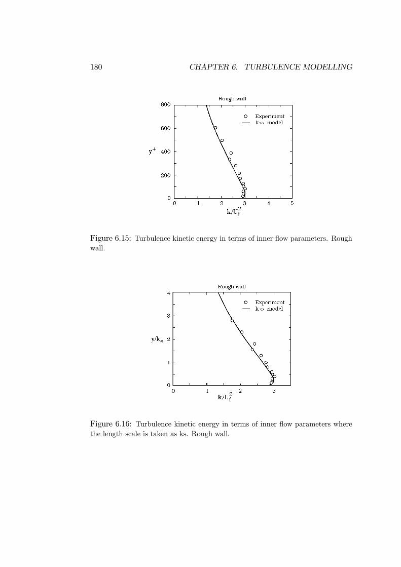
180 CHAPTER 6. TURBULENCE MODELLING
Figure 6.15: Turbulence kinetic energy in terms of inner flow parameters. Roughwall.
Figure 6.16: Turbulence kinetic energy in terms of inner flow parameters wherethe length scale is taken as ks. Rough wall.

6.5. LARGE EDDY SIMULATION (LES) 181
6.5 Large Eddy Simulation (LES)
6.5.1 Model equations
The principal idea in the method of LES is to average the N.-S. equations overa small volume of space. (Recall that the N.-S. equations are averaged overtime to obtain the Reynolds equations, i.e., Eqs. 6.1 and 6.2). Normally, thesize of the averaging volume is chosen such that the small-scale componentof turbulence is, for convenience, not resolved. The aforementioned space-averaging gives the following set of equations: (1) the continuity equation,
∂ui∂xi
= 0 (6.53)
and (2) the equation of motion
∂ui∂t+ uj
∂ui∂xj
= −1ρ
∂p
∂xi+ ν
∂
∂xj(∂ui∂xj
+∂uj∂xi
)−∂uiuj∂xj
(6.54)
in which ui = the space-averaged (the resolved) component of the velocity;p = the space-averaged (the resolved) component of the pressure; and ui =the fluctuating component of the velocity over the averaging volume (calledthe subgrid-scale component of the velocity, to differentiate it from the term”fluctuation” in the conventional Reynolds decomposition), and uiuj = thesubgrid-scale stresses, analogous to the Reynolds stresses in the case of theReynolds decomposition.The subgrid-scale stresses (SGS) are written (by analogy to the Boussi-
nesq approximation)
uiuj = νt(∂ui∂xj
+∂uj∂xi
) (6.55)
in which νt = the turbulence viscosity associated with the unresolved com-ponent of turbulence. (Note that the subgrid-scale stresses in the aboveequation are the off-diagonal part of the subgrid-scale stress tensor. The di-agonal part is automatically included in the pressure term.) Hence, Eq. 6.54will be
∂ui∂t+ uj
∂ui∂xj
= −1ρ
∂p
∂xi+
∂
∂xj(ν + νt)(
∂ui∂xj
+∂uj∂xi
) (6.56)
(It may be noted that the turbulence viscosity νt here is different from thatin the k − ω model defined in the previous section. As emphasized in the

182 CHAPTER 6. TURBULENCE MODELLING
present definition, Eq. 6.55, νt is associated with the unresolved small-scaleturbulence averaged over the ”averaging” volume, while νt defined in con-junction with the k − ω model is associated with the turbulence over theentire spectrum).On dimensional grounds, the turbulence viscosity is written as
νt = C2s∆
2s (6.57)
in which∆ is a length scale and Cs is a nondimensional constant. (By makingan analogy to Prandtl’s mixing-length hypothesis, it may be seen that s mustbe a quantity like ∂u/∂y). We shall return to this point later.Clearly, the resolved quantities, ui(xi, t), p(xi, t) and νt(xi, t) in Eqs. 6.55-
6.57 should be dependent on the size of the averaging volume. The smallerthe size of this volume, the better the resolution (both in space and time),and therefore the more information on space and time variations of ui(xi, t),p(xi, t) and νt(xi, t), implying that these quantities are dependent on thesize of the averaging volume. This feature in LES is handled through νt asfollows.As seen in Eq. 6.57, νt involves a length scale, ∆. This quantity is taken
as the length scale representing the size of the averaging volume
∆ = (∆x1∆x2∆x3)1/3 (6.58)
in which ∆x1, ∆x2, ∆x3 are the grid sizes in the x1−, x2−, x3− directions,respectively. (The averaging volume being considered to be ∆x1∆x2∆x3).Furthermore, the quantity s in Eq. 6.57 is taken as
s = (2SijSij)1/2 (6.59)
in which Sij
Sij =1
2(∂ui∂xj
+∂uj∂xi
) (6.60)
It is easy to see that s can also be written in the following form
s = (∂ui∂xj
+∂uj∂xi
)∂ui∂xj
1/2
(6.61)
The above model (Eqs. 6.53-6.59) is known as the Smagorinsky (1963)model for LES. As seen, only one ”closure” coefficient is required, namely
6.5. LARGE EDDY SIMULATION (LES) 183
Cs, the Smagorinsky constant. The value of the Smagorinsky constant isdetermined from experiments.To sum up, the solution of the above set of equations, namely Eqs. 6.53-
6.55, and Eqs. 6.57-6.60, basically gives the time series of the hydrodynamicquantities (the velocity components and the pressure) in space, similar tothe time series obtained in a laboratory experiment using, for example, theLaser Doppler Anemometer (LDA), or the Particle Image Velocimetry (PIV)techniques. Once we obtain this raw data, then we process the data interms of statistical quantities such as the mean, the variance, other statisticalmoments, and even correlations and spectra, in exactly the same fashion aswe process data from experiments. (It should be added that, clearly, the timeseries obtained through the LES ”experiments” are resolved with a resolutionequal to the grid size selected in the simulation, just as the experimentallyobtained time series are resolved with a resolution equal to the size of themeasurement volume of the measuring instrument, e.g. to the size of themeasurement volume of the LDA probe.)A detailed account of turbulence models for LES has been given in a
review paper by Meneveau and Katz (2000).
6.5.2 An application example
In this subsection, we will present the results of a study where the LES modelwas used to simulate the wave boundary layer in a U-shaped oscillating tunnel(Fig. 6.17); The study is essentially a part of a Ph.D. work conducted at theTechnical University of Denmark, Lohmann et al. (2006). The CFD codeemployed in the study, called NS3, a 3-D numerical flow solver, was madeavailable by DHI Water and Environment.The Smagorinski subgrid-scale model was used in the calculations. Re-
garding the value chosen for the Smagorinski constant,Cs, experience showsthatCs equals 0.2 in isotropic turbulence and 0.1 in channel flow. In Lohmannet al.’s (2006) study, the latter value was found to be most appropriate, basedon comparison with experimental data. The van Driest damping functionf = 1 − exp(−y+
Ad) (see Eq. 6.23) is generally used as a standard part of
the Smagorinski subgrid-scale formation; it was also used in the study ofLohmann et al. (2006) (see p. 3 of the latter publication).Note that the free-stream velocity varies according to
U0 = U0m sin(ωt)

184 CHAPTER 6. TURBULENCE MODELLING
Figure 6.17: U-shaped oscillating tunnel.
in which ω is the angular frequency of the motion, ω = 2πT, T being the
period. (See Chapter 5 for a detailed discussion of wave boundary layers.)
Fig. 6.18 presents the raw time series of the three components of theresolved velocity at three different values of the distance y from the bed. Asseen from Fig. 6.18, the time series is, qualitatively, no different from theones obtained experimentally using LDA (c.f. Fig. 5.7 in Chapter 5).Ensemble averaging is used to calculate the mean value of the resolved
velocity, e.g.,
u(y,ωt) =1
N
N
j=1
u[y, ω(t+ (j − 1)T )] (6.62)
and the root-mean-square (r.m.s.) value of the subgrid-scale component ofthe velocity, e.g., u = u− u,
u 2(y,ωt) =1
N − 1
N
j=1
[u[y, ω(t+ (j − 1)T )]− u(y,ωt)]212
(6.63)
Lohmann et al. (2006) found that, for the chosen phase values, averaging

6.5. LARGE EDDY SIMULATION (LES) 185
Figure 6.18: Time series of velocity components.

186 CHAPTER 6. TURBULENCE MODELLING
Figure 6.19: Sequence of velocity profiles over half period of the motion.
Figure 6.20: Sequence of velocity profiles over half period of the motion. Semi-logplot.

6.5. LARGE EDDY SIMULATION (LES) 187
Figure 6.21: Sequence of turbulence profiles.

188 CHAPTER 6. TURBULENCE MODELLING
Figure 6.22: Shear stress profiles.
first over the x− z plane at a given y−location, and then over 3 periods wassufficient to achieve reliable ensemble averages.Fig. 6.19 gives a sequence of velocity profiles at different phase values ωt
over one half period of the motion. The distance from the wall is normalizedby the amplitude of the free-stream motion, a(= U0mT
2π). The figure also gives
two sets of other data: one from the numerical study of Justesen (1988) wherea turbulence-energy equation model, namely the k− ε model, was used; andthe second from the experimental work of Jensen et al. (1989); the latterhas been described in greater detail in Chapter 5. Fig. 6.19 shows that theLES model does a better job than the k− ε model. In Fig. 6.20, the velocityinformation is plotted on a semi-logarithmic graph. The figure illustrates howthe LES solution behaves for small values of the distance from the bed inrelation to the experimental data. From the figure, although superior to thek − ε model, the LES model underpredicts the velocities for small y values.Figs. 6.21 and 6.22 present the turbulence data obtained by the LES
model along with the experimental data. Although there are discrepanciesbetween the model prediction and the experiment, the model predicts the

6.6. REFERENCES 189
turbulence fairly well. Yet, one must note that the model near the bed failsto some extent to predict the turbulence accurately. This may be a majorshortcoming when processes (to be studied by the model) have significantelements related to the turbulence near the bed, particularly related to they− and z−components of turbulence.
6.6 References
1. Absi, R. (2005): ”Comment on ’Turbulent diffusion of momentum andsuspended particles: A finite-mixing-length theory’ (Physics of Fluids,16, 2342 (2004))”. Physics of Fluids, vol. 17, 079101-079102.
2. Cebeci, T. and Chang, K.C. (1978): ”Calculation of incompressiblerough-wall boundary-layer flows”. AIAA Journal, vol. 16, No. 7,p.730.
3. Dixen, M. (2007): Ph.D. Study. Technical University of Denmark,MEK, Coastal, Maritime and Structural Engineering Section. Ph.D.study is in progress, and undertaken under the supervision of B. M.Sumer and J. Fredsøe.
4. Jensen, B. L., Sumer, B. M. and Fredsøe, J.: ”Turbulent oscillatoryboundary layers at high Reynolds numbers”. Journal of Fluid Mechan-ics, Vol. 206, p. 265, 1989.
5. Justesen, P. (1988): Turbulent wave boundary layers. Series Papers43, Institute of Hydrodynamics and Hydraulic Engineering, Lyngby,Denmark. A Ph.D. study supervised by J. Fredsøe and B.M. Sumer.
6. Lohmann, I.P., Fredsøe, J., Sumer, B.M. and Christensen, E.D. (2006):”Large eddy simulation of the ventilated wave boundary layer”, J. Geo-physical Research, vol. 111, C06036, doi:10.1029/2005JC002946, 1-21.
7. Meneveau, C. and Katz, J. (2000): Scale-Invariance and turbulencemodels for Large-Eddy Simulation. In: Annual Rev. Fluid Mech., vol.32, 1-32.
8. Menter, F. R. 1993 Zonal two equation k-ω turbulence models for aero-dynamic flows. Paper AIAA-93-2906, AIAA 24th Fluid Dynamic Con-ference, July 6-9, 1993, Orlando, Florida.
190 CHAPTER 6. TURBULENCE MODELLING
9. Michelsen, J. A. 1992 Basis3D - a platform for development of multi-block PDE solvers. Technical report, Dept. of Fluid Mechanics, Tech-nical University of Denmark, AFM 92-05, ISSN 0590-8809.
10. Nezu, I. 1977 Turbulent Structure in Open Channel Flows. Ph.D.thesis, Kyoto University, Japan.
11. Nielsen, P. and Teakle, A.L. (2004). ”Turbulent diffusion of momentumand suspended particles: A finite-mixing-length theory”. Physics ofFluids, vol. 16, Number 7, p. 2342.
12. Rodi, W. (1992): ”On the simulation of turbulent flows past bluff bod-ies”. J. Wind Eng., No. 52, August, pp.1-16.
13. Rogallo, R.S. and Moin, P. (1984): ”Numerical simulation of turbulentflows”. Annual Review of Fluid Mechanics, vol. 16, pp. 99-137.
14. Roulund, A. 2000 Three-dimensional modelling of flow around a bottom-mounted pile and its application to scour. Ph.D. thesis, Departmentof Hydrodynamics and Water Resources, Technical University of Den-mark, Supervisors B.M. Sumer, and J. Fredsøe.
15. Roulund, A., Sumer, B.M., Fredsøe, J. and Michelsen, J.: ”Numericaland experimental investigation of flow and scour around a circular pile”.J. Fluid Mechanics, vol. 534, 351-401, 2005.
16. Sørensen, N. N. 1995 General purpose flow solver applied to flow overhills. Ph.D. thesis, Risø National Laboratory, Roskilde, Denmark, Risø-R-827(EN).
17. Sumer, B. M., Chua, L. H. C., Cheng N.-S. & Fredsøe, J. 2003 Theinfluence of turbulence on bedload sediment transport, J. HydraulicEngineering ASCE, 129, No. 8, August Issue.
18. Sumer, B. M., Cokgor, S., & Fredsøe, J. 2001 Suction removal of sedi-ment from between armour blocks. Journal of Hydraulic Engineering,ASCE, 127, No. 4, pp. 293-306, 2001.
19. van Driest, E.R. (1956): ”On turbulent flow near a wall”. J. Aeronau-tical Sciences, vol. 23, p.1007.

6.6. REFERENCES 191
20. Wilcox, D.C. (1994): Turbulence Modelling for CFD. DCW Industries,Inc., La Canada, California, 460 p.
.