B e n d in g D y n a m ic s o f F lu c tu a tin g B io p o...

Bending Dynamics of Fluctuating Biopolymers Probed by AutomatedHigh-Resolution Filament Tracking

Clifford P. Brangwynne,* Gijsje H. Koenderink,* Ed Barry,y Zvonimir Dogic,y Frederick C. MacKintosh,z

and David A. Weitz*§

*Harvard School of Engineering and Applied Sciences, Harvard University, Cambridge, Massachusetts; yRowland Institute at Harvard,Cambridge, Massachusetts; zDepartment of Physics and Astronomy, Vrije Universiteit, Amsterdam, The Netherlands; and §Departmentof Physics, Harvard University, Cambridge, Massachusetts

ABSTRACT Microscope images of fluctuating biopolymers contain a wealth of information about their underlying mechanicsand dynamics. However, successful extraction of this information requires precise localization of filament position and shapefrom thousands of noisy images. Here, we present careful measurements of the bending dynamics of filamentous (F-)actin andmicrotubules at thermal equilibrium with high spatial and temporal resolution using a new, simple but robust, automated imageanalysis algorithm with subpixel accuracy. We find that slender actin filaments have a persistence length of ;17 mm, anddisplay a q!4-dependent relaxation spectrum, as expected from viscous drag. Microtubules have a persistence length of severalmillimeters; interestingly, there is a small correlation between total microtubule length and rigidity, with shorter filamentsappearing softer. However, we show that this correlation can arise, in principle, from intrinsic measurement noise that must becarefully considered. The dynamic behavior of the bending of microtubules also appears more complex than that of F-actin,reflecting their higher-order structure. These results emphasize both the power and limitations of light microscopy techniques forstudying the mechanics and dynamics of biopolymers.

INTRODUCTION

Actin filaments and microtubules are semiflexible biopoly-mers that form the elastic cytoskeletal network within cellsthat controls cell migration, division, cargo transport, andmechanosensing (1). Understanding the mechanical behav-ior of these filaments is thus of central importance forestablishing how they function as a dynamic mechanicalscaffold within living cells. Indeed, mechanical models ofthe cell require accurate measurements of the stiffness anddynamical behavior of the component filaments (2–4).However, the semiflexible macromolecular backbone ofmicrotubules and actin filaments results in physical behaviorthat remains incompletely understood.Using light microscope images to directly measure the

shape fluctuations of individual biopolymers is a powerfultechnique for studying their dynamics and mechanicalbehavior (5–9). By extracting a set of filament coordinatesfrom each image, the variance of the curvature fluctuationsinduced by thermal motion can be used to obtain the bendingrigidity. The rigidity is typically expressed in terms of thelength scale beyond which the filament shows significantcurvature due to thermal forces, known as the persistencelength, lp: Changes in thermally-induced curvature occur ona timescale that is set by viscous drag from the surrounding

fluid. This time can be obtained from the relaxation time of ashape autocorrelation function, such as the mean-squareddifference in curvature calculated for increasing lag times.Utilizing variations of this technique, actin filaments havebeen shown to have a persistence length of;17 mm (5,8,10),although they were initially suggested to have a length scale-dependent rigidity (11). Microtubules have been shown to beorders of magnitude more stiff, with a persistence length onthe order of millimeters (8). However, recent studies havesuggested that microtubule rigidity may depend on theirgrowth velocity (7) and other factors related to their mac-romolecular structure (12–14). Indeed, it was recentlysuggested that inter-protofilament shearing leads to a soft-ening of shorter microtubules (15). Other studies havesuggested that internal dissipation mechanisms may domi-nate over hydrodynamic drag to increase the relaxation timesof microtubules on short length scales (7,16).Successfully extracting such mechanical information from

microscope images is limited by position uncertainties re-sulting from image noise, requiring precise filament tracking.Despite the need for accurate filament localization, reportsutilizing this technique often use semi-manual filamenttracking methods and do not report a noise floor. Automatedvideo tracking of objects with spherical symmetry, such ascolloidal particles and fluorescent point-sources, is a well-developed technique for quantifying their dynamic behavior.Tracking of large numbers of spherical probe particles iscentral to microrheological measurements of the mechanicalbehavior of soft materials such as biopolymer gels and evenliving cells (17–19). Particle tracking algorithms typicallyemploy an initial particle localization, such as intensity

Submitted September 7, 2006, and accepted for publication February 15,2007.

Address reprint requests to David A. Weitz, Gordon Mckay Professor ofApplied Physics and Professor of Physics, Harvard University, Pierce Hall,

Rm. 321, 29 Oxford St., Cambridge, MA 02138. Tel.: 617-496-2842; Fax:

617-495-2875; E-mail: [email protected].

Editor: Marileen Dogterom.

! 2007 by the Biophysical Society

0006-3495/07/07/346/14 $2.00 doi: 10.1529/biophysj.106.096966

346 Biophysical Journal Volume 93 July 2007 346–359

maxima, followed by particle position refinement using anintensity weighted center of mass (20) or fitting to a Gaussianor parabolic function. These algorithms can be used to obtainparticle positions with subpixel accuracy. Positions are thenlinked in time to establish the trajectories of the particles.Precise tracking of objects with nonspherical symmetry,such as biopolymer filaments, presents more of a challenge.Unlike colloidal particles, the shape of the filament is notknown a priori and thus conventional automated fittingtechniques are no longer applicable. There is an extensivecomputer vision literature that describes identification of lin-ear structures, such as roads or capillary tubes, from complexlandscapes (21). A related technique for automated trackingof differential interference contrast (DIC) images of linearstructures such as microtubules has been described (22). Arecent study describes automated tracking of uniformly-sizedfluorescent colloidal rods (23). There are also a number ofpapers describing filament-centroid tracking routines for invitro motility assays of fluorescent actin filaments glidingover myosin-coated surfaces (24,25). However, to our know-ledge there have been no reports describing automatedcontour tracking of fluctuating fluorescent filaments withsub-pixel accuracy.In this paper, we develop and utilize a robust automated

image analysis algorithm for tracking fluorescently-labeledbiopolymer filaments with subpixel accuracy. We first dem-onstrate the accuracy of this technique by tracking im-mobilized fluorescent biopolymers and show that we obtain aroot mean-square precision of ;0.15 pixel (;20 nm), evenas the filaments begin to be photobleached after hundreds ofexposures. We then use this technique to study the shapefluctuations of microtubules and actin filaments at thermalequilibrium down to short length and time scales. Thisallows us to address recent conflicting reports of themechanics and dynamics of biopolymer bending fluctu-ations, particularly those of microtubules. The persis-tence length of actin filaments obtained from ourmeasurements agrees well with previous experiments(5,8,10), lp " 17 mm. We obtain microtubule persistencelengths on the order of a few mm, also in agreement withprevious measurements (7,8,13,14). Our data show aslight correlation between filament length and stiffness,consistent with a recent study (15). However, we dem-onstrate that this correlation can in principle arise frominherent noise limitations that occur even with high precisionmeasurements. Thus, over the range we study, there does notappear to be a systematic dependence of the bending rigidityon length or wavevector, in agreement with other studies(7,8,13,14). However, after a careful analysis of the relax-ation times of the fluctuating normal modes, we findevidence that microtubules do display anomalous bendingdynamics that reflects their more complex molecular struc-ture (26) compared to actin filaments. Although the relax-ation times of fluctuating actin filaments are consistent withsimple viscous drag, for microtubules they are much longer

than expected from hydrodynamic drag on short lengthscales. This effect may be due to a surprisingly large internaldissipation that dominates the relaxation times of microtu-bules on biologically relevant length and time scales. Ourfindings emphasize both the power and limitations of lightmicroscopy techniques for probing the complex mechanicalbehavior of semiflexible polymers.

Filament tracking algorithm

The analysis algorithm used to track the shape of fluo-rescently labeled biopolymers in successive images consistsof the steps detailed below. Briefly, an initial rough estimateof the position of a filament is first determined by thresh-olding the image. Pixels above threshold are then skeleton-ized to obtain a 1-pixel-wide representation of the filament.A polynomial fit to this skeleton is then used to walk alongthe contour of the filament, refining the position estimate byfinding the intensity maximum along perpendicular cutsacross the filament.

Background noise reduction

We first performed an image noise reduction by convolvingeach pixel of the image with a Gaussian kernel over a localregion of size w:

AGauss#x; y$ %1

B#x; y$+w

i;j%!w

A#x1 i; y1 j$exp !i2 1 j2

4

! ";

(1)

where B#x; y$ is an appropriate normalization. The longwavelength background intensity variation is alsoaccounted for by averaging each pixel of the unfilteredimage over a local region of size w, to obtain Abackground#x; y$:The final filtered image is then obtained from: Afilter#x; y$ %abs AGauss#x; y$ ! Abackground#x; y$

# $(20). For initial filament

localization, the size w was set to be around three timeslarger than the width of the filament, ;5 pixels in oursystem. For refinement of the initial filament localization, welimit the convolution of local position information withneighboring position information by setting the filter size toapproximately the width of the filament. An example of theresult of this procedure for a typical image of a fluorescentlylabeled microtubule (Fig. 1 A) is shown in Fig. 1 B. Filtersdesigned specifically for highlighting linear structures areanother alternative (27).

Thresholding

Thresholding was done to separate the filament from theremaining background intensity fluctuations. Pixels with avalue greater than the threshold value are assigned a value of1, whereas those with a value less than the threshold valueare assigned a value of 0. The threshold value is given by

Biopolymer Bending Dynamics 347

Biophysical Journal 93(1) 346–359

f % ÆIijæ1msij; where ÆIijæ is the average intensity value ofall pixels ij, and sij is the standard deviation of the pixelintensity, both of which are dominated by the nonfilamentbackground pixels. For high-frequency image acquisition,the signal/noise ratio (s/n) is usually small; thus, it is criticalto determine an appropriate threshold value by determiningthe number of standard deviations away from the average, m.If m is too small, some background may be included, whereasif it is large, the entire filament may not be included. Wetypically start with a small value of m(;3) and successivelyincrease its value in small increments (0.2) until the backboneof the thresholded region is well fit by a polynomial. Anexample of thresholding is shown in Fig. 1 C.

Skeletonization

For good s/n and an appropriate threshold value, pixelsabove threshold will cover the fluorescent filament in acluster several pixels wide. This cluster can be thinned to a1-pixel-wide line using a skeletonization routine that erodespixels while maintaining cluster connectedness (28). Skel-etonization has the advantage that small clusters correspond-ing to nonfilament background fluctuations above thresholdare typically eliminated by the erosion process. Persistentfluorescent specks that are still not eliminated are ignoredusing a simple routine to exclude objects above thresholdfrom specific regions of the image. If necessary, morecomplex pixel clustering algorithms may be used to identifypixels associated with the desired filament (28). An exampleof skeletonization of a thresholded filament is shown in Fig.1 D. This line, corresponding to a set of position coordinates

x % i, y % j such that Iij % 1; provides a first, imprecise,estimate of the filament location.

Polynomial fitting and filament rotation

We refine the initial position estimate by analyzing the inten-sity distribution of sections taken perpendicular to the localslope of the filament (Fig. 2 A). To obtain the local slope,we fit the xy coordinates of the skeleton with a polynomialof order p. The polynomial degree required depends on theamount of curvature in the filaments under study; wetypically use p % 3–5 for microtubules and actin filaments.We thus obtain a curve f #x$ % +p

i%0 cixi that can be dif-

ferentiated to obtain an estimate of the local slope of the

filament at position x0: u#x0$ % tan!1 dfdxjx%x0

: To obtain the

FIGURE 1 Example of the initial image processing stages of the filament

localization algorithm for a typical fluorescence micrograph of an Alexa-488dye-labeled microtubule constrained to move in a quasi-two-dimensional

chamber. (A) Unprocessed image, and image after bandpassing, as in Eq.

1 (B), followed by thresholding (C), and skeletonization (D). Note that thespurious speck in the thresholded image is eliminated upon skeletonization.

FIGURE 2 Example of filament position refinement by fitting Gaussianintensity profiles along cuts perpendicular to the filament contour. (A)Skeleton (see Fig. 1 D) in the xy coordinate frame with polynomial fit and

schematic perpendicular cuts. (B) The intensity profile along a perpendicularcut of an unprocessed image is shown (solid squares). After bandpassing theimage, the intensity distribution (open squares) is fit to a Gaussian (solidline). The filament location is taken to be the maximum of the Gaussian.

348 Brangwynne et al.


intensity profile of the filament perpendicular to this localslope, we rotate the original image by an angle u#x0$ aroundthe position, !xrot % #xo; f #xo$$; to orient the filament hor-izontally. Successful image rotation requires the use of agood interpolation algorithm that maps the intensity of allpixels onto the rotated image without introducing artifacts.Image rotation routines implementing good interpolationalgorithms accompany software packages such as IDL andMatlab. The process is computationally intensive, and thuswe restrict image rotation to a local region of interest aroundthe filament with coordinates &#x0!b$ : #x01b$;#f #x0$!b$ :#f #x0$1b$'; where b is larger than the extent of the Gaussiankernel, w.Because the skeletonization procedure erodes pixels at the

ends of the thresholded filament, we sample perpendicularsections along the polynomial backbone from, typically, 4pixels before to 4 pixels after the end points of the skeleton.We calculate the integrated signal along the perpendicularcolumn of pixels k, M % +k Ik; and set a threshold value(‘‘masscut’’) for identified filament positions. The first andlast filament positions with a signal mass above thresholddefine the two ends of the filament. Because fluorescentlylabeled biopolymers frequently display nonuniform labelingalong their length, masscut thresholding often leaves holes inthe position identification of the filament, particularly inlow-s/n images. We fill in these gaps by linear interpolationbetween the nearest successfully sampled points.

Position refinement by Gaussian fitting

We proceed to analyze the intensity distribution of thevertical column of pixels in each rotated region. An exampleof such an intensity distribution is shown in Fig. 2 B (solidsquares). By applying the Gaussian convolution kernel andbackground subtraction to this rotated local region, weimprove the s/n ratio by eliminating both high- and low-frequency noise (Fig. 2 B, open squares). The center of thefilament can be identified from this intensity distributionusing either functional fitting or an intensity-weighted centerof mass. It is important to note that the Gaussian filter leadsto averaging of pixel intensities over a local region definedby the size of the Gaussian kernel (;5–10 pixels); averagingthe filament centroid obtained from adjacent perpendicularcuts of unbandpassed images could provide an alternative s/nimprovement, without undesirable averaging in the perpen-dicular direction. We choose to fit the intensity distributionto a Gaussian intensity profile (Fig. 2 B, solid line), whichyields the highest precision for tracking of spherical objects(29). We find that the primary advantage of Gaussian fittingover an intensity-weighted center-of-mass approach is itsrelative insensitivity to any residual background signal.The position of the center of the Gaussian, y9g; identifiesthe position of the filament in the rotated frame. This centerposition is then mapped back onto the unrotated full imagecoordinate system to obtain the real-space position of the

mth sampled point !xm; using ym% f #x0$1f&y9g! f #x0$'3cos#u#x0$$g and xm% x0!f&y9g! f #x0$'3sin#u#x0$$g: Thisprocedure is repeated along the polynomial at the desiredsampling frequency, typically in steps of size Ds%2 pixels,until a full set of refined filament coordinates is obtained.

MATERIALS AND METHODS

Monomeric (G) actin was purified from rabbit skeletal muscle (30), with an

additional gel-column chromatography step (Sephacryl S-200) to removeresidual cross-linking and capping proteins. Actin filaments stabilized with

phalloidin were prepared by polymerizing G-actin in AB-buffer (25 mM

imidazole, 50mMKCl, 2mMMgCl2, 1mMEGTA, and 1mMdithiothreitol,

pH 7.4). Filaments were fluorescently labeled by using Alexa-488-modifiedG-actin, or by stabilizing unlabeled actin filaments withAlexa-488 phalloidin

(Molecular Probes). We analyzed actin filaments with contour lengths

between 8 and 15 mm. Tubulin was purified from bovine brain according tostandard procedures and fluorescently labeled with Alexa-488. Microtubules

were polymerized in K-Pipes buffer (80 mM K-Pipes, 1 mM EGTA, and

1 mMMgCl2, pH 6.8) at 37"C and stabilized with 10 mM taxol.

Microtubules were imaged in a quasi-two-dimensional sample chamberthat was made by placing a small volume (typically 0.3 mL) of a dilute

solution of stabilized filaments augmented with a standard antioxidant

mixture (glucose oxidase, catalase, glucose, 2-mercaptoethanol) (31) to slow

photobleaching between a microscope slide and coverslip. The edges ofthe coverslip were sealed with mineral oil to prevent fluid flow due to

evaporation. Adsorption of filaments onto the glass surfaces was avoided by

passivating the glass with adsorbed bovine serum albumin or covalently

attached poly-(ethylene glycol) chains (MPEG-silane-5000, Nektar, SanCarlos, CA). All experiments were performed at room temperature.

Fluorescent images of microtubules were acquired on a Leica DM-IRB

inverted microscope equipped with either a Hamamatsu intensified charge-coupled device (CCD) camera C7190-21 (exposure time 33 ms, 0.136 mm/

pixel) or a Hamamatsu ORCA CCD camera C4742-95 (exposure time 59

ms, 0.128 mm/pixel) (Hamamatsu City, Japan). Images of actin filaments

and some microtubules were obtained using a Nikon inverted microscopewith Coolsnap HQ camera (exposure time of 5–100 ms, 0.129–0.194 mm/

pixel). Microtubules were also imaged with a 10-ms exposure using a high-

speed camera (Phantom V7, Vision Research, Wayne, NJ) equipped with an

image intensifier (Model VS4-1845HS, Video Scope International, Dulles,VA). Some actin filament bending data (see Fig. 7) was obtained using a

second method to slow down the filament dynamics by adding nonadsorbing

polymer (2–3%, Dextran 500,000 g/mol). The polymer induces an attractivedepletion interaction between the coverglass and the filaments, leading to

confinement of the filaments close to the bottom surface. Using these

samples, we were able to acquire images with either epi-illumination or total

internal reflection fluorescence (TIRF) illumination. Due to the low levels ofbackground fluorescence, we were able to decrease exposure time with TIRF

illumination to a few milliseconds.

The data in Fig. 11 B were fit to a line to obtain a slope of !0.050 60.066, indicating no statistically significant correlation between persistencelength, lp; and wavevector, q. In addition, the correlation coefficient was

calculated using r % slpq=slpsq;where slpq is the covariance between lp andq, and slp and sq is the standard deviation of lp and q, respectively. Thevalues of r vary from 1 (strongly correlated) to !1 (strongly anticorrelated).We obtained a value of !0.096, which is a statistically insignificant

correlation (p . 0.005).

RESULTS

Evaluation of tracking precision

As a first test to evaluate the performance of our algorithmwe determined the uncertainty in filament localization



arising from camera shot noise and tracking limitations. Thiswas accomplished by analyzing the shape fluctuations ofmicrotubules that were immobilized by physically adheringthem to poly-L-lysine coated surfaces. These microtubuleswere locked tightly to the glass coverslip surface, so anyresidual filament shape fluctuations that we measured wouldbe due to uncertainty in filament localization inherent in ourtechnique. To visualize the typical noise level, we overlaythe extracted shapes of an immobilized filament for 10consecutive frames of a movie in Fig. 3. The insets showhigher-magnification views of two representative positionsalong the filament against a pixel-sized grid. This explicitlydemonstrates that we obtained subpixel tracking accuracywith a noise level of;0.1–0.2 pixels (;20 nm). This degreeof accuracy is representative of the filaments we track in typ-ical conditions, although, as we quantify below, the trackingaccuracy decreased with decreasing s/n. Since sphericallysymmetric colloidal particles are much more straightforwardto track, and typically result in ;0.1-pixel accuracy, our fil-ament tracking algorithm performed well, with a comparableroot mean-squared (RMS) noise level.

Bending rigidity of microtubules and actinfilaments from mode analysis

We track microtubules and actin filaments freely fluctuating inquasi-two-dimensional chambers. We obtain the filamentbending rigidities by analyzing the shape fluctuations using aFourier decomposition technique developed in previous stud-ies (8,9). From the pixel coordinates #xm; ym$ of the filamentswe first calculate the tangent angle u#s$ as a function ofarclength s, using: u#sm$ % tan!1#ym11 ! ym$= #xm11 ! xm$;where

sm % +m!1

j%0

%%%%%%%%%%%%%%%%%%%%%%%%%%%%%%%%%%%%%%%%%%%%%%%%%#xj11 ! xj$2 1 #yj11 ! yj$2

q( )

1 1=2%%%%%%%%%%%%%%%%%%%%%%%%%%%%%%%%%%%%%%%%%%%%%%%%%%%%%%#xm11 ! xm$2 1 #ym11 ! ym$2

q:

The tangent angle is then decomposed into a sum of cosines,

u#s$ %%%%2

L

r+N

n%0

aq cos#qs$; (2)

where the wave vector q is defined as q % np=L; with n themode number and L the filament contour length (8). A cosineexpansion of the tangent angle using different normalizationprefactors has been used in other studies (9), but we find thenormalization used by Gittes et al. most natural since it re-sults in a length-independent variance of the mode ampli-tude. Use of this pure cosine mode decomposition assumes azero-curvature boundary condition at the free filament ends,appropriate for freely fluctuating filaments.The amplitudes, aq; of the first 24 bending modes of a

freely fluctuating microtubule are plotted as a function oftime in each of the subpanels of Fig. 4. The microtubule has anonzero intrinsic curvature, u0#s$ %

%%%%%%%%2=L

p+N

n%0 a0q cos#qs$;

resulting in a nonzero mean amplitude. The variance of thelower modes contains information about the flexural rigidity,whereas the amplitude of the higher modes is dominated byexperimental noise. The amplitudes of these higher modeswiden with time (Fig. 4, inset) due to photobleaching andconcomitant reduction of the s/n.A convenient feature of the cosine expansion in Eq. 2 is

that random noise due to errors in filament localization obeysthe following simple relation (8):

FIGURE 3 Filament contours for a microtubule fixed to an oppositely

charged, poly-L-lysine-coated glass surface. (Insets) Higher-magnificationviews of 10 consecutive filament contours from a video acquisition; the pixel

size is represented by the gray grid, demonstrating that the filament tracking

algorithm performs with subpixel accuracy.

FIGURE 4 The amplitude of 24 bendingmodes for the microtubule shownin Fig. 1, plotted as a function of time in each of the subpanels. The micro-

tubule has intrinsic curvature, resulting in a nonzero mean amplitude. The

variance of the lower modes contains information about the flexural rigidity,

whereas the amplitude of the higher modes is dominated by experimentalnoise. The amplitudes widen with time (see inset) due to photobleaching andconcomitant reduction of the signal/noise ratio.



Æ#a0

q ! aq$2ænoise %4

Le2 11 #N ! 2$sin2 np

2#N ! 1$

! "& '; (3)

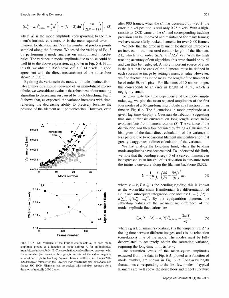
where a0q is the mode amplitude corresponding to the fila-ment’s intrinsic curvature, e2 is the mean-squared error infilament localization, and N is the number of position pointssampled along the filament. We tested the validity of Eq. 3by performing a mode analysis on immobilized microtu-bules. The variance in mode amplitude due to noise could bewell fit to the above expression, as shown in Fig. 5 A. Fromthis fit, we obtain a RMS error

%%%%e2

p" 0:14 pixels, in good

agreement with the direct measurement of the noise floorshown in Fig. 3.By fitting the variance in themode amplitude obtained from

later frames of a movie sequence of an immobilized micro-tubule, wewere able to evaluate the robustness of our trackingalgorithm to decreasing s/n caused by photobleaching. Fig. 5B shows that, as expected, the variance increases with time,reflecting the decreasing ability to precisely localize theposition of the filament as it photobleaches. However, even

after 900 frames, when the s/n has decreased by ;20%, theerror in pixel position is still only 0.25 pixels. With a high-sensitivity CCD camera, the s/n and corresponding trackingprecision can be improved and maintained for many frames;we have successfully tracked filaments for over 7000 frames.We note that the error in filament localization introduces

an increase in the measured contour length of the filament,DL, which is of order DL=L " e2=Ds2 (8). With the hightracking accuracy of our algorithm, this error should be,1%and can thus be neglected. A more important source of erroris the fact that the ends of the filaments must be defined ineach successive image by setting a masscut value. However,we find fluctuations in the measured length of the filament tobe of order dL " 1 pixel. For filaments of 10 mm or longer,this corresponds to an error in length of ,1%, which isnegligibly small.To investigate the time dependence of the mode ampli-

tudes, aq; we plot the mean-squared amplitudes of the firstfour modes of a 30-mm-long microtubule as a function of lagtime in Fig. 6 A. The fluctuations in mode amplitude at agiven lag time display a Gaussian distribution, suggestingthat small intrinsic curvature on long length scales helpsavoid artifacts from filament rotation (8). The variance of thedistribution was therefore obtained by fitting a Gaussian to ahistogram of the data; direct calculation of the variance isless precise due to occasional filament misidentification thatgreatly exaggerates a direct calculation of the variance.We first analyze the long-time limit, where the bending

mode amplitudes have decorrelated. To understand this limit,we note that the bending energy U of a curved filament canbe expressed as an integral of its deviation in curvature fromthe intrinsic curvature along the filament backbone (8,32):

U % 1

2k

Z L

0

@u

@s! @u0

@s

! "2

ds; (4)

where k % kBT3 lp is the bending rigidity; this is knownas the worm-like chain Hamiltonian. By differentiation ofEq. 2 and subsequent integration, one obtains: U % #1=2$3k+N

n%1 q2#a0q ! aq$2: By the equipartition theorem, the

saturating values of the mean-square difference of themode amplitude fluctuations are

Æ#aq#t1Dt$ ! aq#t$$2æt;Dt(t %2kBT

kq2 ; (5)

where kB is Boltzmann’s constant, T is the temperature, Dt isthe lag time between different images, and t is the relaxation(correlation) time of the mode. The modes must be fullydecorrelated to accurately obtain the saturating variance,requiring the long-time limit Dt ( t:The saturation levels of the mean-square amplitudes

extracted from the data in Fig. 6 A, plotted as a function ofmode number, are shown in Fig. 6 B. Long-wavelengthfluctuations corresponding to the first few modes of typicalfilaments are well above the noise floor and reflect curvature

FIGURE 5 (A) Variance of the Fourier coefficients aq of each modeamplitude plotted as a function of mode number n, for an individual

immobilizedmicrotubule. (B) The error in filament localization increaseswith

frame number (i.e., time) as the signal/noise ratio of the video images is

reduced due to photobleaching. Squares, frames 0–200; circles, frames 200–400, triangles, frames 400–600, inverted triangles, frames600–800,diamonds,frames 800–1000. Filaments can be tracked with subpixel accuracy for a

duration of typically 2000 frames.



fluctutions due to thermal energy. The saturating amplitudesof the first few modes scale with the expected q!2 depen-dence of Eq. 5 (Fig. 2 B, solid line). Higher modes cannot beused if their relaxation timescale, t; is similar to or shorterthan the exposure time texp (5–100 ms in our studies). Thefluctuations of these modes are effectively blurred, causingthem to appear stiffer. We were able to extend the mea-surable q range to higher q values by using short exposuretimes, either with TIRF illumination (33,34), or by using ahigh-speed camera equipped with an intensifier. As ex-pected, for data acquired using short exposure times, theregime displaying the expected q!2 dependence is extended,as demonstrated in Fig. 7.We obtain the persistence length of filaments by fitting the

saturating mean-square amplitude versus q to Eq. 5. The fits

were extended over the range of modes for which no sys-tematic deviation below q!2 was observed, i.e., texp ) t(typically, the first three to five modes). From these fits, wefind a persistence length lp of 17.06 2.8mm (mean6 SD) foractin filaments, in good agreement with previous studies(5,8,10). This persistence length is independent of the lengthof the actin filaments within the observed range of 8–15 mm,as shown in Fig. 8 A. In contrast, for microtubules, we finda small apparent correlation between lp and length: shortfilaments tend to appear softer, as shown in Fig. 8 B.Microtubules with lengths between 25 and 66 mm have anaverage persistence length of 2.8 6 1 mm (mean 6 SD),similar to previously reported values (7,8,14) (Fig. 8 B).Shorter filaments with lengths in the range 18–25 mm have alower average persistence length of 1.5 6 0.7 mm. The dataare thus in qualitative agreement with a recent reportsuggesting that the internal protofilament structure of micro-tubules leads to a bending rigidity that depends on totalmicrotubule length (15). Indeed, our data can be fit reasonablywell to the reported functional form of this dependence lp %lNp &11 Lcrit=L# $2'!1; with lNp % 4:5 mm; and Lcrit % 30 mm;as shown by the dashed line in Fig. 8 B. However, the closeproximity of the noise floor both in our measurements (Fig. 8B, dotted line) and in those of Pampaloni et al. (15) suggest acautious interpretation of these results.

Bending relaxation timescales

By using a Fourier decomposition of the filament shape,we can readily determine mode relaxation times from theautocorrelation function, as shown in Fig. 6 A. However,these Fourier modes are only approximations of the truenormal modes of the dynamical equation of motion (seeAppendix). Although a Fourier decomposition is suitable fordetermining the static behavior, as described above, Fouriermodes are not normal modes of the system. Instead, Fouriermodes will reflect the combined behavior of different normalmodes relaxing on different timescales. Nevertheless, the

FIGURE 6 (A) Time dependence of

the mean-square amplitude of Fourier

coefficients aq of the first four bendingmodes of a 30-mm -long microtubule,

with fits to Eq. 6. (Inset) Note that datascale together when plotted as a func-

tion of the scaled variables MSD#aq$=MSD#aq$plateau and t/t. (B)Mean-square

amplitudes of the Fourier coefficients aqplotted as a function of mode number n,for increasing lag times Dt % 0.059 s,

0.0177 s, and 5.9 s. At longer lag times,

the variance of the amplitude for the first

few modes approaches the expectedq2-dependence of Eq. 6, with a persis-

tence length of 4 mm (decreasing solidline). At higher mode numbers, the am-

plitudes are dominated by a RMS noiseof 0.15 pixel (increasing solid line).

FIGURE 7 Saturation values of the mean-square amplitudes of the bend-

ing modes of 12 actin filaments imaged using different ratios of exposure

time to mode relaxation time. Light gray squares were imaged with 100 msexposure in aqueous buffer, gray triangles were imaged with 100 ms ex-

posure time in a viscous background solution. Black circles were imaged

with 5–10 ms exposure time using TIRF illumination. The onset of deviation

from q2-scaling (black line, slope 1/lp % 17 mm) corresponds to wavevectorsfor which the relaxation time roughly equals the exposure time; fluctuations

for larger wavevectors are blurred and register as smaller values.



Fourier modes are a convenient basis set that completelycaptures the instantaneous filament shape. It is thereforepossible to express the true normal-mode amplitudes interms of our measured amplitudes aq#t$; and thus to measurethe normal-mode relaxation rates. A more complete descrip-tion of this procedure is provided in the Appendix.Surprisingly, we found that over all experimentally

accessible timescales, mode-mixing effects arising from thefact that these Fourier modes are not pure normal modeswere small. This can be understood as follows. By symme-try, the odd (even) Fourier modes decompose into only odd(even) normal modes Jl: Strictly speaking, this means thatthe amplitudes in Eq. 5 for finite Dt exhibit non-single-exponential relaxation. For the lowest Fourier modes, n % 1,2; however, only the corresponding l % 1, 2 normal modes

are apparent at later stages of relaxation, since the higher-order normal modes relax more quickly. A comparisonbetween the first Fourier mode and the corresponding normalmode of a microtubule is shown in Fig. 9 A. The relaxationtimes obtained from fits to a single exponential are verysimilar: 0.84 s for the Fourier mode and 0.82 s for the normalmode. For the higher Fourier modes, n % 3, 4. . . , thefilament end effects are less apparent, and the normal modesare better approximated by Fourier modes. However, asdiscussed in the Appendix, since these modes mix with moreslowly decaying modes the non-single-exponential behaviormay be apparent at longer times in the relaxation. Neverthe-less, these non-single-exponential corrections can be shown tobe of order 10–15%. Thus, in practice, the dynamical behaviorof the cosine modes is well approximated by the single-exponential relaxation of the normal modes:

Æ#aq#t1Dt$ ! aq#t$$2æt % #1! e!Dt=t$2kBT

kq2 : (6)

As shown in the appendix, the mode relaxation times t aregiven by:

t ’ g

kq4

*; (7)

where q* " #n11=2$p=L: The hydrodynamic drag coeffi-cient for a rod confined between two surfaces is approxi-mated by

g " 4ph

ln2h

a

! ";

where h is the buffer viscosity, h is the distance between thefilament and the coverslips (;1 mm), and 2a is the filamentdiameter (8,10). The mean-square fluctuation of the modeamplitudes can indeed be well fit to Eq. 6 (Fig. 6 A, lines).The collected data for the relaxation times t of 26

microtubules and 22 actin filaments, obtained from fits to Eq.6, are shown in Fig. 9. For actin filaments (circles), the re-laxation times decay rapidly with q*; consistent with theexpected q!4

* -dependence. We fit the data to Eq. 7; using theaverage persistence length, lp % 17:0 mm; we obtain a dragcoefficient of gactin % 9:4 mPa+s, in reasonable agreementwith the calculated value of 1.8 mPa+s obtained from theapproximate hydrodynamic expression. The inset shows thenormalized relaxation timescales, tkq4*; which are roughlyconstant. This indicates that the bending relaxation timescalefor actin filaments is set by hydrodynamic drag. The relax-ation timescales of microtubules show a similar behavior(Fig. 9, squares) at the smallest wavevectors, with the re-laxation times decreasing rapidly as t " q!4

* : However, atlarger wavectors, the relaxation times are much larger thanexpected and appear to become wavevector-independent.Data taken with faster acquisition time also show this trend,although some points remain consistent with a simple t "q!4* scaling, suggesting that the dynamic behavior of micro-

tubules is heterogeneous.

FIGURE 8 Persistence length of 22 actin filaments and 26 microtubules

plotted as a function of filament length. (A) Actin filaments show a relatively

narrow distribution of persistence lengths with an average lp % 17:0 6 2:8mm (dashed line). There does not appear to be any dependence on filamentlength over the range studied. (B) Microtubules display a broader dis-

tribution of persistence lengths, and there is an apparent small correlation

between the bending rigidity and filament length, with shorter filaments

appearing softer. Our data can be fit to a length-dependent expression forthe persistence length, lp % lNp &11 Lcrit=L# $2'!1; with lNp % 4:5 mm; and

Lcrit % 30 mm; as shown by the dashed line (15). However, the dotted line,

denoting a conservative estimate of the intrinsic noise limitations, suggeststhat this correlation may only reflect a noise limitation.



For microtubules, a similar deviation from q!4* -depen-

dence was recently reported for the relaxation times ofthermally fluctuating microtubules clamped at one end (7). Apossible explanation for the origin of these anomalous relaxa-tion times comes from a recent study (16) that incorporatesan additional friction term in the Langevin equation (seeAppendix), describing the bending dynamics of thermallyfluctuating biopolymers:

k@4u

@s41 g

@u

@t1 g9

@

@t

@4u

@s4

! "% f #s; t$: (8)

This additional third term represents internal frictionwithin the biopolymer. The mode relaxation times (Eq. 7)now become:

t % g1 g9q4

*

kq4

*; (9)

where g9=a4 can be considered an effective internal viscosity.Equation 9 implies that at wavevectors larger than qc;#g=g9$1=4; internal friction will dominate and the relaxation timescorrespondingly become q*-independent. The microtubule re-laxation time data can befit to Eq. 9, as shown in Fig. 9B; usingthe average persistence length, lp % 2.5 mm, we obtain a dragcoefficient of gMT % 8:3 mPa+s, in fair agreement with thevalue of 2.4 mPa+s estimated from the approximate hydrody-namic expression. From the fit, we also obtain an internaldissipation ofg9 % 163 10!25 N +m2 + s , corresponding to aninternal viscosity of g9=a4MT " 107 mPa+s. Interestingly, thisvalue is similar to that obtained in the previous study,g9 % 6:93 10!25 N +m2 + s (7) (fit shown in Fig. 9 B, inset).Thus, in both cases, microtubules appear to cross over to awavevector-independent relaxation regime at qc " 0:3mm!1;on a length scale corresponding to l " 20 mm.

Microtubules in cells

Our tracking algorithm can also be extended to extract thecontours of fluorescently labeled microtubules within livingcells. Because the cytoskeleton of living cells is typically

packed with a dense network of microtubules with a mesh sizeof ;1 mm, initial filament localization using a thresholding/skeletonization routine is insufficient. However, with a graph-ical interface that enables the user to provide an initial estimateof the filament position, it is possible to implement our simplealgorithm with minor modifications. Alternatively, the initialfilament localization may be accomplished with automatededge-detection routines (21). A modification for handlingfilament intersections must also be added to our algorithm forcomplex networks. This can be accomplished by introducing ax2 goodness-of-fit parameter for theGaussianfit to the intensityprofile of the filament cross-section. In this way, filamentintersections, for which the intensity profile is poorly fit to aGaussian, can be easily distinguished from nonoverlappingsegments of the filament. Such filament positions can then beinterpolated between neighboring sampled positions. In Fig.10, we demonstrate that we can track a single microtubulethrough the dense network in a fixed tissue-culture cell usingsuch an approach (4).

DISCUSSION

We have developed and characterized a simple but robustalgorithm for precisely tracking fluorescent filaments. Tostudy biopolymer bending dynamics using this algorithm,we took care to identify and characterize the main sources oferror that arise in these measurements.

1. Intrinsic noise makes the bending fluctuations appearlarger and therefore makes the filament look softer.

2. Correlated fluctuations appear to have a smaller variancethan uncorrelated fluctuations evaluated at longer times,and thus cause error since the filament appears stiffer.

3. Long exposure times relative to relaxation time can causethe filament to blur, making the fluctuations appearsmaller and, thus, the filament appear stiffer.

4. Improper mode decomposition can lead to mode-mixingeffects that hinder interpretation of the dynamic behaviorof filaments.

FIGURE 9 (A) Comparison betweenthe decorrelation of the first Fourier

mode (green squares) and the corre-

sponding normal mode (blue circles)of the microtubule shown in Fig. 6 A.The normal mode was obtained from a

sum of odd Fourier modes, as described

in the Appendix. The relaxation timeobtained from a fit to a single expo-

nential is 0.84 s for the Fourier mode

and 0.82 s for the normal mode. (B)Relaxation times of bending modes ofactin filaments (circles) and microtu-

bules (squares) plotted as a function of

wavevector q*: Solid symbols represent

data obtained using short exposure times (5–10 ms). The data for actin filaments are consistent with a q!4* dependence (solid line) expected from simple

hydrodynamic drag (Eq. 7). For microtubules, we find a deviation from q!4* at q* . 0:3mm!1 (solid line, fit to Eq. 9; dotted line, fit to q!4

* ). The inset shows the

same data normalized as tkq4* plotted versus q*: Black crosses are data for microtubules from Janson and Dogterom (7).



Each of these sources of error can affect measurements ofbending rigidity and/or relaxation time, and need to becarefully considered.

Filament bending rigidity

Using our precise tracking algorithm, we determine thepersistence length and relaxation timescales of thermallyfluctuating actin filaments and microtubules. Consistent withprevious studies, we find that microtubules are two orders ofmagnitude stiffer than actin filaments. Both actin filaments andmicrotubules show a wavevector dependence of their bendingamplitude that agreeswellwith expectations fromthewormlikechain model. Actin filaments have a persistence length of;17mm, independent of filament length. Interestingly, for micro-tubuleswefind aweak dependence on the filament length, withshort microtubules appearing softer than long ones.The persistence lengths plotted in Fig. 8, A and B, are

essentially averages over multiple q-values, since they areobtained by fitting multiple bending modes to Eq. 5 (see Fig.6 B). Thus, the apparent length dependence of the bendingrigidity of microtubules in Fig. 8 B could actually reflect a

q-dependence. To test this, we plot the persistence lengthobtained from the variance of each mode as a function of thecorresponding wavevector, as shown in Fig. 11 A. Althoughthere does not appear to be a strong correlation at smallwavevector, high-wavevector fluctuations indeed appear tobe softer. These soft high-wavevector modes would tend tomake shorter filaments appear softer, since their relativecontribution to the average stiffness (obtained from a fit ofmultiple modes to Eq. 5) would be larger. One possibleexplanation for this wavevector dependence is that atsufficiently high wavevectors, mode amplitude fluctuationsdue to filament tracking noise dominate over thermalbending fluctuations. This is unlikely, however, since modesin the noise regime obey the noise relationship (Eq. 3) that iseasily identifiable, as illustrated in Fig. 6 B. Moreover, weonly considered modes that clearly decorrelated with lagtime, which is never true for modes in the noise regime.Thus, the high wavevector fluctuations we measure are notdirectly affected by intrinsic noise fluctuations.Although intrinsic noise does not directly contribute to the

measured fluctuations, it is possible that noise still indirectlyaffects the measurements, since it introduces a bias: highwavevector fluctuations can be detected above the noise flooronly if the filament is sufficiently soft. This effect is likely toarise for microtubules in particular because of the largefilament-to-filament variability of the persistence length.Indeed, using conservative values for the noise floor (takingan RMS noise of 0.5 pixel), an estimate of the location of thisbias agrees with the trend in Fig. 11 A (solid line). Furthersupport for this comes from the fact that within individualfilaments there is no detectable wavevector dependence ofthe bending rigidity, as can be seen in the rescaled data inFig. 11 B. As expected from the plot, linear regression showsno statistically significant correlation. Interestingly, althoughour data are consistent with the findings of Pampaloni et al.(15), intrinsic noise biasing likely contributes to the smallcorrelation we find between total filament length and rigidity,as shown by the corresponding noise boundary in Fig. 8 B.Indeed, such artifacts introduced by noise limitations could

FIGURE 10 Fluorescence image of a monkey kidney epithelial cell that

has been fixed and stained, showing microtubules near the cell edge. Wetrack one microtubule by combining the automated filament tracking

algorithm with a manual initial filament identification. On the right is the

fluorescence image with the filament coordinates overlaid in red.

FIGURE 11 Persistencelengthofmi-

crotubulebendingmodesas a functionofthe correspondingwavevectorq. (A) Thepersistence length appears to be lower at

higherwavevectors, but this is likely dueto a bias caused by intrinsic noise

limitations. The dotted line denoting

the noise-limited regime was obtained

using conservative values for the noisefloor (RMS error of 0.5 pixel) in Eq. 3.

(B) Within individual filaments, there is

no dependence of the persistence length

obtained from each mode (normalizedby the persistence length averaged over

all modes) on wavevector (normalized

by the wavevector averaged over all

modes). Each filament is shown with adifferent symbol.



also contribute to the bending rigidity/length correlationfound in this recent study. Further experimental work in-corporating a careful analysis of the noise will be required todetermine whether there is indeed a significant dependenceof the rigidity on microtubule length, and to elucidate theprecise origin of this potentially interesting finding (15).

Bending relaxation timescales

By studying the time evolution of the mode amplitudes, wefound that actin filaments display relatively simple bendingdynamics, whereas microtubule bending reflects a morecomplex mechanical behavior. The relaxation times of actinfilaments are consistent with the q!4

* -wavevector depen-dence expected from hydrodynamic drag. Microtubules,however, appear to cross over from a hydrodynamically-dominated relaxation regime at long length scales, l. 20mmto a wavevector-independent relaxation regime at shorterlength scales, l, 20mm:These anomalous relaxation timescales do not appear to be

due to any of the sources of measurement error we identified.In particular, if high-wavevector relaxation timescales wereaffected by the exposure time of the camera, then therelaxation timescales would become smaller and not larger,as we have observed. We addressed the possibility of ex-posure time effects by obtaining data using much shorterexposure times (Fig. 9 B, solid symbols). These data showa similar trend, although some points remain consistent witha simple q!4

* scaling. Although the actin relaxation time-scale data show a very slight deviation from a perfectq!4* -dependence possibly due to measurement errors, for

microtubules the marked spread in the data showing devi-ation from the expected q!4

* -dependence does not appear toresult from measurement error, and highlights the heteroge-neity of the dynamic behavior of microtubules.As discussed above, it was recently suggested that

structural changes in the form of interprotofilament shearinglead to a filament-length-dependent stiffness (15). Interest-ingly, the model described there would seem to lead to areduced effective stiffness, and therefore reduced relaxationrate for short wavelength modes. However, we find noevidence for a true wavevector-dependent rigidity (Fig. 11).Moreover, the strong trend in our microtubule relaxationtime data could not be explained by the small stiffness biaswe observe, since the normalized relaxation times (Fig. 9,inset) remain consistent with a wavevector-independentrelaxation regime. The anomalous microtubule relaxationtimes thus appear to reflect some form of viscous dissipationwithin a heterogeneous population of microtubules.To estimate the dissipative parameter g9 in Eq. 8, we adopt

a simple physical picture for the microtubules (16). For anelastic filament composed of a porous or viscoelastic gel-likematerial, internal dissipation results from the flow of a fluidof viscosity h9 through pores of size j: This leads tog9 % h9a6=j2; where 2a is the filament diameter. Wave-

vector-independent relaxation times for bulky mitotic chro-mosomes appear to be described by such a picture (16).Because the diameter of microtubules is ;25 nm, whereasactin filaments are a more slender 7 nm, similar internaldissipation should be more apparent for microtubules; this isqualitatively consistent with our findings. However, thehigh-frequency rheology of actin solutions (35–37) shows noevidence of deviations from pure hydrodynamic drag up tofrequencies as high as 100 kHz, corresponding to relaxationtimes up to four orders of magnitude smaller than formicrotubules in this study. This fact cannot be explained bythe difference between microtubule and actin diametersalone. Specifically, the bending moduli of both microtubulesand actin are consistent with the simple prediction k % Ea4

of elasticity theory, where the Young’s modulus E " 1 GPafor both. Thus, the model above for porous filaments wouldresult in a relaxation rate of order h9#a=j$2=E: It seems morelikely that anomalously large values of g9 for microtubules,as compared with actin, are due to slow structural fluctua-tions or conformational changes (16).

CONCLUSIONS

We have demonstrated that bending fluctuations of fluo-rescently-labeled biopolymers can be tracked with highspatial and temporal resolution using a simple and robustautomated subpixel tracking algorithm. Using this algorithm,we confirmed previous studies reporting a persistence lengthof actin filaments of ;17 mm, and microtubule persistencelengths on the order of a few millimeters. For microtubules,we found that a correlation between persistence length andfilament length can arise due to biasing from intrinsic noiselimitations. By studying the time evolution of actin bendingfluctuations, we found that their relaxation times display aq!4* hydrodynamic scaling, whereas some microtubules

appear to transition into a high-wavevector regime domi-nated by surprisingly large internal viscous dissipation.These results emphasize the heterogeneous mechanical be-havior of microtubules, and suggest that microtubulesdisplay anomalous bending dynamics that reflect their com-plex molecular structure.

APPENDIX

To understand the time dependence of the mode amplitude fluctuations (Fig.

6 A), we consider the following Langevin equation for changes in the

transverse position u(s,t) of the filament as a function of arclength, s, andtime, t (5,8,10,38):

k@4u

@s41 g

@u

@t% f #s; t$: (A1)

The first term accounts for the elastic restoring force prescribed by Eq. 4, the

second term is the hydrodynamic drag on the filament as it moves through

the viscous buffer, and the third term is the d-function correlated randomthermal noise acting along the filament.



Following Aragon and Pecora (38), we find solutions to the equation of

motion (Eq. A1) in terms of normal modes jl#s$; which are solutions to the

eigenvalue equation

k@4jl@s4

% lljl; (A2)

with the boundary conditions corresponding to no net forces or torques on

the ends,

@2jl@s2

% @3jl@s3

% 0: (A3)

Here, the eigenvalues are given by ll % k#al=L$4; where cos#al$ cosh#al$ %1: To within better than 0.4%, the solutions of the latter are approximatelygiven by al , #l 1 1=2$p for l $ 1; where this approximation becomes in-

creasingly accurate for the higher modes. Thus, even though the al will

appear raised to the power of four in the expressions below, we will make

no more than ;1.5% error using the approximation above.The solutions to Eq. A2 are orthogonal. Thus, we can construct an

orthonormal basis for functions on #!L=2;L=2$; given by

jl %

1%%%L

p 3cos#als=L$cos#al=2$

1cosh#als=L$cosh#al=2$

& 'For l % 1; 3; 5 . . .

1%%%L

p 3sin#als=L$sin#al=2$

1sinh#als=L$sinh#al=2$

& 'For l % 2; 4; 6 . . .

8>><

>>:

(A4)

The solutions we seek can be expressed as

u#s; t$ % +N

l%1

Jl#t$jl#s$: (A5)

The Langevin equation can also be written now in terms of the amplitudes

Jl#t$ %Zjl#s9$u#s9; t$ds9 and fl#t$ %

Zjl#s9$f #s9; t$ds9

gd

dtJl % !llJl 1 fl: (A6)

The solutions to this are of the form

Jl#t$ % Jl#0$e!vlt 1e!vl t

g

Z t

0

evlt9fl#t9$dt9 (A7)

for t $ 0: This allows us to calculate the correlation functions

ÆJl#t$Jm#0$æ % ÆJl#0$Jm#0$æe!vl t; (A8)

since Æfl#t$Jm#0$æ % 0: However, given the time translation invariance of

this result, as well as the nondegenerate spectrum of relaxation rates

vl % ll=g; this only makes sense if ÆJl#t$Jm#0$æ % 0 for all l 6% m: Thiscan also be seen from the fact that the bending energy

k

2

Z@2u

@s2

! "2

ds % 1

2+l

llJlJl; (A9)

which results in Gaussian distributed amplitudes

ÆJlJmæ %kT

ll

dlm: (A10)

Here, we have used partial integration for the bending energy, together with

the force- and torque-free boundary conditions.

Of course, we could have also used the more familiar Fourier modes

bn#s$ %%%%2

L

rsin

pn

L&s1 L=2'

( ); (A11)

but only for the statics. These are not normal modes for the dynamics. The

Fourier amplitudes Bn#t$ %Rbn#s9$u#s9; t$ds9 now satisfy

ÆBnBmæ %kT

fn

dnm; (A12)

where this is an equal-time correlation function and fn % k#pn=L$4:We note that the last two terms of Eq. A1 both depend on the local

position/velocity of the polymer. As these variables are nonlocal in the

tangent angle variables, it is not possible to write this Langevin equation in

terms of u(s). However, for weakly bending filaments, the local slope of thefilament u#s; t$ % du#s; t$=ds can also be used to describe the shape. This

shape can be further described by the Fourier amplitudes above:

an %Z

gn#s9$u#s9; t$ds9; (A13)

where

gn#s$ %%%%2

L

rcos

pn

L&s1 L=2'

( ): (A14)

In terms of the normal modes, the amplitudes an#t$ can be expressed as

an#t$ % +N

l%1

Jl#t$Z

gn#s$d

dsjl#s$ds: (A15)

We define the matrix

Mnl %Z

gn#s$d

dsjl#s$ds: (A16)

Thus, the correlation of amplitudes an#t$ can be found in terms of the normal

modes:

Æan#t$an#0$æ % +N

l%1

ÆJl#t$Jl#0$æ#Mnl$2 % +N

l%1

kT

ll

#Mnl$2e!vl t:

(A17)

We note that the functions gn#s$ are alternately odd and even, whereas thefunctions jl#s$ are alternately even and odd. Thus, Mnl % 0; unless n and lare either both odd or both even. For example, LM1l % 7.05, 0, 5.69, 0, 5.66,

0, for l % 1, 2, . . . 6, whereas LM3l % !0.377, 0, 12.29, 0, 6.21, 0, for l % 1,

2, . . . 6.Alternatively, the matrix inverse M!1 can be used to express the normal

mode amplitudes Jl in terms of the measured amplitudes an:

Jl#t$ % +N

m%1

#M!1$lmam#t$; (A18)

so that

ÆDJl#t$2æ [ Æ&Jl#t$ !Jl#0$'2æ % +N

m%1

ÆDam#t$2æ##M!1$lm$2

% kT

ll

#1! e!vl t$: (A19)

Since the matrices describing the linear transformations between Jl and anare easily evaluated, this procedure provides a practical way to determine the

normal-mode relaxation spectrum in terms of the an that can be measured as

discussed above.



For large l, the dominant term in this sum is for m % l, since the effect ofthe ends of the filament become negligible in this limit. Thus, we expect that

for large enough n, the relaxation of an is approximately single-exponential

with relaxation rate

vn , k#&n1 1=2'p=L$4=g: (A20)

At the other end of the spectrum, for n% 1, 2, the relaxation of an will also beapproximately single-exponential with relaxation rate vn for long times,since the most slowly relaxing mode in Eq. A17 is for l % n when n % 1, 2.

The corrections to this approximate single-exponential behavior, due

to modes l % n 1 2, both have amplitudes smaller by approximatelyln=ln12 % &#n1 1=2$=#n1 5=2$'4 and relax substantially faster (specifi-

cally, by a factor of ln12=ln). Using the matrix entries Mnl above, we find

that the second term in Eq. A17 is smaller than the first by a factor of 0.022

(0.036) for n % 1 (2). Perhaps surprisingly, even though the n % 3, 4 modesmix with the slowly relaxing l % 1, 2 normal modes in Eq. A17, using the

Mnl above, we find the relative contribution of these slow modes to be 0.027

and 0.048, respectively. Including other subdominant terms in Eq. A17, we

expect that it is sufficient to keep only the l% n term, to within;10–15%. Thisexplains why we find little evidence, in practice, for non-single-exponential

relaxation for any of the modes we examined. We have directly implemented

the procedure described above for several data sets for n % 1–6 and find thatthe correction is within our error bars. However, accounting for the correct

normal mode relaxation using Eq. A20 is essential for interpretation of the

dynamics of both microtubules and F-actin in our experiments.

We thank T. Mitchison and Z. Perlman for their kind donation of tubulin

and their assistance with fluorescent labeling. We also thank L. Mahadevan

for helpful discussions.

This work was supported by the National Science Foundation (DMR-

0602684 and CTS-0505929), the Harvard Materials Research Science andEngineering Center (DMR-0213805), the Harvard Integrative Graduate

Education and Research Traineeship on Biomechanics (DGE-0221682),

and the Stichting voor Fundamenteel Onderzoek der Materie/Nederlandse

Organisatie voor Wetenschappelijk Onderzoek. G.H.K. is supported by aEuropean Marie Curie Fellowship (FP6-2002-Mobility-6B, Contract No.

8526).

REFERENCES

1. Alberts, B., A. Johnson, J. Lewis, M. Raff, K. Roberts, and P. Walter.2006.Molecular Biology of the Cell, 4th ed. Academic Press, NewYork.

2. Mackintosh, F., J. Kas, and P. Janmey. 1995. Elasticity of semiflexiblebiopolymer networks. Phys. Rev. Lett. 75:4425–4429.

3. Gardel, M. L., J. H. Shin, F. C. MacKintosh, L. Mahadevan, P.Matsudaira, and D. A. Weitz. 2004. Elastic behavior of cross-linkedand bundled actin networks. Science. 304:1301–1305.

4. Brangwynne, C. P., F. C. MacKintosh, S. Kumar, N. A. Geisse, J.Talbot, L. Mahadevan, K. K. Parker, D. E. Ingber, and D. A. Weitz.2006. Microtubules can bear enhanced compressive loads in livingcells because of lateral reinforcement. J. Cell Biol. 173:733–741.

5. Ott, A., M. Magnasco, A. Simon, and A. Libchaber. 1993. Measure-ment of the persistence length of polymerized actin using fluorescencemicroscopy. Phys. Rev. E. 48:R1652–R1645.

6. Venier, P., A. C. Maggs, M. F. Carlier, and D. Pantaloni, 1994.Analysis of microtubule rigidity using hydrodynamic flow and thermalfluctuations. J. Biol. Chem. 269:13353–13360.

7. Janson, M. E., and M. Dogterom. 2004. A bending mode analysis forgrowing microtubules: evidence for a velocity-dependent rigidity.Biophys. J. 87:2723–2736.

8. Gittes, F., B. Mickey, J. Nettleton, and J. Howard. 1993. Flexuralrigidity of microtubules and actin filaments measured from thermalfluctuations in shape. J. Cell Biol. 120:923–934.

9. Kas, J., H. Strey, J. X. Tang, D. Finger, R. Ezzell, E. Sackmann, andP. A. Janmey. 1996. F-actin, a model polymer for semiflexible chainsin dilute, semidilute, and liquid crystalline solutions. Biophys. J. 70:609–625.

10. Le Goff, L., O. Hallatschek, E. Frey, and F. Amblard. 2002.Tracerstudies on f-actin fluctuations. Phys. Rev. Lett. 89:258101.

11. Kas, J., H. Strey, and E. Sackmann. 1993. Direct measurement of thewave-vector-dependent bending stiffness of freely flickering actinfilaments. Europhys. Lett. 21:865–870.

12. Mickey, B., and J. Howard. 1995. Rigidity of microtubules is increasedby stabilizing agents. J. Cell Biol. 130:909–917.

13. Kikumoto, M., M. Kurachi,V. Tosa, and H. Tashiro. 2006. Flexuralrigidity of individual microtubules measured by a buckling force withoptical traps. Biophys. J. 90:1687–1696.

14. Felgner, H., R. Frank, and M. Schliwa. 1996. Flexural rigidity ofmicrotubules measured with the use of optical tweezers. J. Cell Sci.109:509–516.

15. Pampaloni, F., G. Lattanzi, A. Jonas, T. Surrey, E. Frey, and E. L.Florin. 2006. Thermal fluctuations of grafted microtubules provideevidence of a length-dependent persistence length. Proc. Natl. Acad.Sci. USA. 103:10248–10253.

16. Poirier, M. G., and J. F. Marko. 2002. Effect of internal friction onbiofilament dynamics. Phys. Rev. Lett. 88:228103.

17. Gardel, M. L., M. T. Valentine, J. C. Crocker, A. R. Bausch, and D. A.Weitz. 2003. Microrheology of entangled F-actin solutions. Phys. Rev.Lett. 91:158302.

18. Lau, A. W. C.,B. D. Hoffman, A. Davies, J. C. Crocker, and T. C.Lubensky. 2003.Microrheology, stress fluctuations, and active behav-ior of living cells. Phys. Rev. Lett. 91.198101

19. Gittes, F., B. Schnurr, P. D. Olmsted, F. C. Mackintosh, and C. F.Schmidt. 1997. Microscopic viscoelasticity: shear moduli of softmaterials determined from thermal fluctuations. Phys. Rev. Lett. 79:3286–3289.

20. Crocker, J. C., and D. Grier. 1996. Methods of digital video mi-croscopy for colloidal studies. J. Colloid Interface Sci. 179:298–310.

21. Steger, C. 1998. An unbiased detector of curvilinear structures. IEEETrans. Pattern Anal. Mach. Intell. 20:113–125.

22. Danuser, G., P. T. Tran, and E. D. Salmon. 2000. Tracking differentialinterference contrast diffraction line images with nanometre sensitivity.J. Microsc. 198:34–53.

23. Mohraz, A., and M. J. Solomon. 2005. Direct visualization of colloidalrod assembly by confocal microscopy. Langmuir. 21:5298–5306.

24. Hamelink, W., J. G. Zegers, B. W. Treijtel, and T. Blange. 1999. Pathreconstruction as a tool for actin filament speed determination in the invitro motility assay. Anal. Biochem. 273:12–19.

25. Work, S. S., and D. M. Warshaw. 1992. Computer-assisted tracking ofactin filament motility. Anal. Biochem. 202:275–285.

26. Nogales, E. 2000. Structural insights into microtubule function. Annu.Rev. Biochem. 69:277–302.

27. Jacob, M., and M. Unser. 2004. Design of steerable filters for featuredetection using canny-like criteria. IEEE Trans. Pattern Anal. Mach.Intell. 26:1007–1019.

28. Russ, J. C. 1998. The Image Processing Handbook, 3rd ed. CRC press& IEEE press, Boca Raton, FL.

29. Cheezum, M. K., W. F. Walker, and W. H. Guilford. 2001.Quantitative comparison of algorithms for tracking single fluorescentparticles. Biophys. J. 81:2378–2388.

30. Pardee, J. D., and J. A. Spudich. 1982. Purification of muscle actin.Methods Enzymol. 85:164–181.

31. Uhde, J., M. Keller, E. Sackmann, E. Parmeggiani, and E. Frey. 2004.Internal motility in stiffening actin-myosin networks. Phys. Rev. Lett.93:268101.

32. Landau, L. D., and E. M. Lifshitz. Theory of Elasticity, 3rd ed. 1986,Pergamon Press, Oxford, U.K.



33. Kuhn, J. R., and T. D. Pollard. 2005. Real-time measurements of actinfilament polymerization by total internal reflection fluorescencemicroscopy. Biophys. J. 88:1387–1402.

34. Axelrod, D. 2003. Total internal reflection microscopy in cell biology.Methods Enzymol. 361:1–33.

35. Koenderink, G. H., M. Atakhorrami, F. C. Mackintosh, and C. F.Schmidt. 2006.High-frequency stress relaxation in semiflexible poly-mer solutions and networks. Phys. Rev. Lett. 96:138307.

36. Gisler, T., and D. A. Weitz. 1999. Scaling of the microrheology ofsemidilute f-actin solutions. Phys. Rev. Lett. 82:1606–1609.

37. Schnurr, B., F. Gittes, F. C. Mackintosh, and C. F. Schmidt. 1997.Determining microscopic viscoelasticity in flexible and semiflexiblepolymer networks from thermal fluctuations. Macromolecules. 30:7781–7792.

38. Aragon, S. R., and R. Pecora. 1985. Dynamics of wormlike chains.Macromolecules. 18:1868–1875.



B e n d in g D y n a m ic s o f F lu c tu a tin g B io p o...

Documents

Transcript of B e n d in g D y n a m ic s o f F lu c tu a tin g B io p o...