IOP PUBLISHING FLUID DYNAMICS RESEARCH

Fluid Dyn. Res. 41 (2009) 051405 (16pp) doi:10.1088/0169-5983/41/5/051405

INVITED PAPER

Azimuthal instability of a vortex ring computed by avortex sheet panel method

Hualong Feng1, Leon Kaganovskiy2 and Robert Krasny3

1 School of Science, Nanjing University of Science and Technology, Nanjing, Jiangsu 210094,People’s Republic of China2 Department of Natural Sciences, New College of Florida, Sarasota, FL 34243, USA3 Department of Mathematics, University of Michigan, Ann Arbor, MI 48109, USA

E-mail: krasny@umich.edu

Received 31 December 2007, in final form 23 February 2009Published 2 September 2009Online at stacks.iop.org/FDR/41/051405

Communicated by Y Fukumoto

AbstractA Lagrangian panel method is presented for vortex sheet motion in three-dimensional (3D) flow. The sheet is represented by a set of quadrilateral panelshaving a tree structure. The panels have active particles that carry circulationand passive particles used for adaptive refinement. The Biot–Savart kernel isregularized and the velocity is evaluated by a treecode. The method is appliedto compute the azimuthal instability of a vortex ring, starting from a perturbedcircular disc vortex sheet initial condition. Details of the core dynamics areclarified by tracking material lines on the sheet surface. Results are presentedshowing the following sequence of events: spiral roll-up of the sheet into aring, wavy deformation of the ring axis, first collapse of the vortex core ineach wavelength, second collapse of the vortex core out of phase with the firstcollapse, formation of loops wrapped around the core and radial ejection ofringlets. The collapse of the vortex core is correlated with converging axialflow.

1. Introduction

Vortex rings are readily formed by ejecting fluid from a circular nozzle. At early times thering maintains axisymmetry, but at later times it often undergoes a wavy azimuthal instabilityand abrupt transition to turbulence. A detailed understanding of this process is still beingpursued by many investigators. The present work is concerned with numerical simulation ofthe azimuthal instability using a vortex sheet model for the ring. Comprehensive reviews onvortex rings were given by Shariff and Leonard (1992) and Lim and Nickels (1995). First, webriefly recall some of the relevant prior results, starting with experiments and proceeding totheory and numerical simulations.

© 2009 The Japan Society of Fluid Mechanics and IOP Publishing Ltd Printed in the UK0169-5983/09/051405+16$30.00 1

Fluid Dyn. Res. 41 (2009) 051405 Hualong Feng et al

Experimental visualization of the azimuthal instability must contend with the fact that thering translates in space as the instability develops, but nonetheless many detailed features havebeen revealed. Maxworthy (1977) found that axial flow develops along the core of the ring dueto azimuthal pressure gradients arising from non-uniform breakdown of the azimuthal waves.Glezer and Coles (1990) inferred that secondary vortex tubes with alternating circulation arewrapped around the core of the ring. Weigand and Gharib (1994) observed vortex sheddingfrom the periphery of the ring accompanied by a stepwise decrease in ring circulation. Naitohet al (2002) found that the deformation of the ring axis is correlated with axial flow in thecore. Dazin et al (2006a, 2006b) documented many aspects of the linear and nonlinear stagesof the instability, including the presence of secondary dipole structures in slices through thering.

Theoretical analysis of the azimuthal instability is complicated by the curvature of thering axis, but the case of a straight vortex tube offers a starting point. For example, Mooreand Saffman (1975) performed a stability analysis of a vortex tube in an external strain field.From such studies emerged the idea that the azimuthal ring instability involves a competitionbetween the irrotational strain induced by distant portions of the ring and the self-inducedrotation of the core. Widnall and co-workers presented a series of papers culminating in thework of Widnall and Tsai (1977), which gave predictions for the instability wavenumber,growth rate and mode structure in good agreement with experiment. Saffman (1978) studiedthe effect of the core vorticity profile and derived a formula for the instability wavenumberas a function of Reynolds number. Recent work by Fukumoto and Hattori (2005) showed thatthe ring’s self-induced dipole field may have an even greater effect than the strain field indestabilizing the ring.

Numerical simulation of the azimuthal ring instability has been carried out using finite-differences (e.g. Archer et al 2008, Shariff et al 1994) and vortex methods (e.g. Bergdorfet al 2007, Cocle et al 2008, Knio and Ghoniem 1990). In most cases the initial condition is atoroidal core to which a perturbation is applied. The present work instead uses a vortex sheetmodel encompassing the spiral roll-up by which the core of the ring is formed. In addition,we use free-space boundary conditions (i.e. the velocity vanishes far from the ring) instead ofthe periodic boundary conditions common in previous simulations.

Vortex methods were reviewed by Cottet and Koumoutsakos (2000). A numericalmethod for tracking vortex sheet motion in three-dimensional (3D) flow requires a discreterepresentation of the sheet, a quadrature scheme for evaluating the Biot–Savart integral andan adaptive refinement scheme to maintain resolution as the sheet rolls up. Triangulationsare often used to represent the sheet surface (e.g. Agishtein and Migdal 1989, Brady et al1998, Pozrikidis 2000, Stock 2006, Stock et al 2008), but filament representations have alsobeen employed (e.g. Ashurst and Meiburg 1988, Lindsay and Krasny 2001, Sakajo 2001). Avariety of quadrature and adaptive refinement schemes have been developed, and this is stillan active area of research.

The present approach uses a Lagrangian panel method that builds on previous work,but also incorporates some new techniques (Kaganovskiy 2006, 2007, Feng 2007). Panelmethods are often used in aerodynamics to treat unsteady free vortex sheets as well as boundvortex sheets on solid surfaces (Katz and Plotkin 2001). Here, we regularize the Biot–Savartkernel and use a treecode to evaluate the velocity, following Lindsay and Krasny (2001), butinstead of the filament representation used there, we employ a panel representation that ismore effective in resolving the deformed sheet surface. Each panel is a quadrilateral patchwith respect to Lagrangian coordinates. The set of all panels has a quadtree structure distinctfrom the octtree structure used in the treecode. The panels have active particles that carrycirculation and passive particles used for adaptive refinement. The refinement scheme tests

2

Fluid Dyn. Res. 41 (2009) 051405 Hualong Feng et al

each panel for deformation and if necessary subdivides the panel into four subpanels. Newparticles are inserted by interpolation with respect to Lagrangian coodinates (Krasny 1987).The quadrature scheme evaluates the circulation element using differences of the flow map.The numerical method is local in the sense that it requires little communication betweenneighboring panels.

The method is applied to compute the azimuthal instability of a vortex ring, startingfrom a perturbed circular disk vortex sheet initial condition. Details of the core dynamicsare clarified by tracking material lines on the sheet surface. Results are presented showingthe following sequence of events. Initially the edge of the sheet rolls up into a spiral core,effectively forming a perturbed vortex ring. While this is happening, the azimuthal wavessteepen, leading to a collapse of the core in each wavelength. Afterward, a second collapseoccurs out of phase with the first collapse, accompanied by the formation of loops wrappedaround the core and radial ejection of ringlets. The collapse of the vortex core is correlatedwith converging axial flow, possibly as in the experiments of Naitoh et al (2002). Slicesthrough the sheet surface reveal dipole structures, possibly resembling those observed byDazin et al (2006a, 2006b).

The paper is organized as follows. Section 2 presents the vortex sheet evolution equation.Section 3 describes the numerical method. Section 4 presents numerical results. Conclusionsare given in section 5.

2. Vortex sheet evolution equation

Following Caflisch (1988) and Kaneda (1990), we present the evolution equation for vortexsheet motion in 3D flow. The starting point is the Biot–Savart integral for the velocity inducedby a vortex sheet,

u(x) =∫

SK (x, y) × d!( y), (1)

where S is the sheet surface, d! is the vector-valued circulation element on the sheet and

K (x, y) = − x − y4π |x − y|3

(2)

is the Biot–Savart kernel. Note that

d! = (n × U)dS, (3)

where n is a unit normal vector on the sheet, U is the jump in velocity across thesheet and dS is a scalar area element on the surface. In computations it is advantageousto regularize the kernel and we employ the form suggested by Rosenhead (1930) andMoore (1972),

K δ(x, y) = − x − y4π(|x − y|2 + δ2)3/2

, (4)

where δ is a smoothing parameter. Chorin and Bernard (1973) used a similar approach tocompute vortex sheet motion in 2D flow.

We assume the sheet is a parametrized surface,

x = x(α, β, t), (5)

3

Fluid Dyn. Res. 41 (2009) 051405 Hualong Feng et al

(b)(a) (c)

Figure 1. Schematic of circular disk vortex sheet: (a) vortex filaments, (b) panel representation,(c) azimuthal angles θ1 = π

8 mod π4 (solid lines), θ2 = 0 mod π

4 (dashed lines).

with Lagrangian coordinates α, β. We also refer to x(α, β, t) as the flow map of the vortexsheet. Caflisch (1988) and Kaneda (1990) derived the following expression for the circulationelement,

d! =(

∂'

∂α

∂x∂β

− ∂'

∂β

∂x∂α

)dα dβ, (6)

where ' = '(α, β) is the scalar circulation on the sheet and the Lagrangian derivatives of theflow map, ∂x/∂α, ∂x/∂β, account for vortex stretching. In the present application to vortexrings, the vortex filaments are assumed to be closed curves and we take α = ', β = θ , wherethe circulation is normalized so that 0! ' ! 1 and θ is an angle variable along the filamentswith 0! θ ! 2π . This yields

d! = ∂x∂θ

d'dθ (7)

as a special case of equation (6). Finally, we have the vortex sheet evolution equation,

∂x∂t

=∫ 2π

0

∫ 1

0K δ(x, x̃) × d!̃, (8)

a form of equation (1) expressing the idea that the sheet advects in its self-induced velocityfield.

3. Numerical method

In this section, we describe first the panel representation of the vortex sheet, then thequadrature and adaptive refinement schemes, and finally some coding details.

3.1. Panel representation

Consider Cartesian coordinates x = (x, y, z), where the z-direction is vertical. Figure 1adepicts a circular disc vortex sheet defined by

x =√

1 − '2 cos θ, y =√

1 − '2 sin θ, z = 0, (9)

where 0! ' ! 1, 0! θ ! 2π . The sheet is comprised of circular vortex filaments, i.e. lineson which the circulation ' is constant. Equation (9) corresponds to the bound vortex sheet

4

Fluid Dyn. Res. 41 (2009) 051405 Hualong Feng et al

= =

=

=

(a) (b)

xd

xc

xa

xb

Figure 2. Definition of a panel. (a) Panel in Lagrangian coordinate space with vertices a, b, c, dand (b) the same panel in physical space with vertices xa, xb, xc, xd . Arrows indicate panel edgescorresponding to vortex filaments.

in potential flow past a circular disk, and if the sheet is allowed to roll up, it forms anaxisymmetric vortex ring (Taylor 1953). The initial condition for the simulation includesa perturbation in the z-coordinate, leading to a non-axisymmetric ring. Figure 1(b) is aschematic of the panel representation of the sheet. A panel is a quadrilateral patch on the sheetsurface with particles at the vertices. The panels cover the sheet and the set of all panels hasa quadtree structure created by adaptive refinement, as explained below. For future reference,in figure 1(c) we define two sets of azimuthal angles, θ1 ≡ π

8 mod π4 and θ2 ≡ 0 mod π

4 ; in theexample computed later below, θ1 corresponds to the crests and θ2 corresponds to the troughsof the perturbation in the direction of ring propagation.

Figure 2 gives more detail about the definition of a panel. Figure 2(a) depicts a panel inLagrangian coordinate space with vertices a, b, c, d . A panel is a rectangle with sides parallelto the coordinate axes, so that either ' = constant or θ = constant on each edge. The linesof constant ', indicated by arrows, correspond to vortex filaments. Figure 2(b) depicts thepanel in physical space with particles xa, xb, xc, xd at the vertices. The particles are advectedin physical space and the panel retains its definition as a rectangular patch in Lagrangiancoodinate space.

3.2. Quadrature scheme

Let xi , i = 1 : N denote the set of all particles on the sheet. We need to explain how theparticle velocities are computed. The method is conceptually simple; the integral over thesheet surface in equation (8) is replaced by a sum over panels and the integral over each panelis evaluated by a 2D trapezoid rule. This leads to a discretization of the form

dxi

dt=

N∑

j=1

K δ(xi − xj ) × wj , (10)

where wj is the weight associated with particle xj . The weights are given in terms of thecirculation elements d! and we refer to figure 2 to explain how these are computed. Oneapproach, based on equation (7), has the general form

d! ≈(

∂x∂θ

)

v

· ('d − 'a)(θb − θa), (11)

5

Fluid Dyn. Res. 41 (2009) 051405 Hualong Feng et al

(b)(a)

xi

xi

Figure 3. Assigning particle weights, two cases. (a) Particle xi receives weight from panelsp1, p2, p3, p4, and (b) particle xi receives weight from panels p5, p6.

(c)(a) (b)

Figure 4. Adaptive refinement scheme: (a) a panel has active particles (•) and passive particles (◦),(b) the original panel has been subdivided into four subpanels and (c) adjacent panels can resideat different levels of subdivision; the particle labeled ©• is passive for the left panel and active forthe two right subpanels of which it is a vertex.

where (∂x/∂θ)v is a finite-difference approximation to the partial derivative of the flow mapat a given vertex v of the panel. This approach was employed by Kaganovskiy (2006), buthe used a finite-difference formula requiring information from neighboring panels to compute(∂x/∂θ)v and found that accuracy was lost as the sheet surface became increasingly deformed.Feng (2007) proposed a simple alternative,

d! ≈( xb + xc

2− xa + xd

2

)('d − 'a), (12)

which does not require information from neighboring panels, and this is the form used here.Hence the vertices of the panel are assigned weights

wa = wb = wc = wd = 14 d!, (13)

where d! is given by equation (12). The factor 14 amounts to applying a 2D trapezoid rule for

the integral over a panel.Note that each panel gives rise to particle weights in this manner. The code therefore

loops over the panels and assigns weight to the panel vertices. Figure 3 depicts two cases.The typical case is that a particle receives weight from four panels (figure 3(a)), but someparticles receive weight from only two panels (figure 3(b)). This concludes our discussion ofthe particle weights in equation (10).

3.3. Adaptive refinement scheme

At this point we note that the code actually advects two types of particles, denoted active andpassive. The active particles are the ones dealt with up to now and the passive particles are anew type used for adaptive refinement. Figure 4(a) shows a panel with active particles (•) at

6

Fluid Dyn. Res. 41 (2009) 051405 Hualong Feng et al

(a) (b)

Figure 5. Distances in physical space used to flag panels for refinement. (a) d1: chord length ofedge and (b) d2: distance from passive particle to chord midpoint.

the vertices and passive particles (◦) at the midpoints of the edges and the panel interior. Weemphasize that these are midpoints with respect to Lagrangian coordinates. For example withreference to the panel in figure 2, a passive particle at the midpoint of edge ab has Lagrangiancoordinates (', θ) = ('a,

12 (θa + θb)), and in physical space it lies somewhere on the arc xa xb.

The active particles contribute circulation to the quadrature scheme through equation (12), aspreviously described. The passive particles do not contribute circulation, but instead enableus to account for panel curvature in the refinement scheme. We explain their role below.

When a panel is flagged for refinement, it is subdivided into four subpanels as infigure 4(b). In this case, the passive particles in the original panel become active particles in thesubpanels, and new passive particles are inserted in the subpanels by quadratic interpolationwith respect to Lagrangian coordinates. For example, along the panel edge where ' = 'a ='b in figure 2, there are two active particles (with θ = θa, θb) and one passive particle (withθ = 1

2 (θa + θb)); this information is used to insert passive particles at the midpoints of thesubpanel edges by quadratic interpolation with respect to θ . Also note that the code allowsadjacent panels to reside at different levels of subdivision, as in figure 4(c). In this case theparticle labeled ©• is passive for the left panel and active for the two right subpanels of whichit is a vertex.

Finally we need to explain how a panel is flagged for refinement. This is done by testingthe panel edges using the distances in physical space defined in figure 5. For each edge wecompute d1 (chord length) and d2 (distance from passive particle to chord midpoint). If d1

or d2 exceeds a user-specified tolerance, the panels on either side of the edge are subdivided.Distance d1 acts in regions where the sheet is being stretched and distance d2 acts in regionsof high curvature. This concludes our discussion of the adaptive refinement scheme.

3.4. Coding details

As explained above, the sheet is represented by a set of panels and particles. A particle hasCartesian coordinates xi = (xi , yi , zi ), Lagrangian coordinates ('i , θi ) and quadrature weightwi , and the code uses global linear arrays to store this information. There is also a quadtreedata structure for the panels, with each node containing information about a given panel, e.g.level of the panel in the quadtree, pointers to subpanels, flags for panel refinement and indicesin the global particle arrays of the particles belonging to the panel. The panel quadtree iscreated at time t = 0 and is updated at each time step by the refinement scheme.

Each edge belongs to two adjacent panels (except for edges on the boundaryof the sheet) and when a new passive particle is inserted on an edge, that information needs tobe communicated to the two panels on either side of the edge. To find these panels, a recursivesearch of Lagrangian coordinate space is performed using a bisection method. The costof the search is logarithmic in the number of panels.

7

Fluid Dyn. Res. 41 (2009) 051405 Hualong Feng et al

t=0

t=1

t=2

t=3

t=4

t=5

t=6

t=7

t=8

Figure 6. Vortex sheet roll-up into a vortex ring. The panels representing the sheet surface areplotted as a wire mesh.

The code was written in Fortran90. There are two components, a main programand the treecode subroutine. The main program controls input, output, timestepping andrefinement. The treecode subroutine computes the velocity of the particles using the methoddescribed by Lindsay and Krasny (2001). The Fortran90 treecode subroutine is based oncode for electrostatics (Johnston). The quadtree structure of the panels is distinct from theocttree structure of the particle clusters in the treecode. The results are visualized usingTecplot.

4. Numerical results

The panel method was applied to compute an example of vortex sheet roll-up into a vortexring. A perturbation of the form z = ar2coskθ was imposed on the circular disk vortex sheet inequation (9), where (r, θ) are polar coordinates on the unperturbed sheet (the factor r2 ensuresthat the perturbation is concentrated near the edge of the disk). The perturbation amplitude wasa = 0.1 the azimuthal wavenumber was k = 8, the smoothing parameter was δ = 0.1 and thefourth-order Runge–Kutta method with (t = 0.05 was used for timestepping. The tolerancesfor panel refinement were d1 ! 0.2 (chord length) and d2 ! 0.02 (midpoint-chord distance).The treecode used pmax = 8 (maximum order), ε = 10−5 (error tolerance) and N0 = 1000(maximum number of particles in a leaf of the tree). Refinement tests were performed toensure that the results are well-resolved. The initial condition has eight-fold symmetry andalthough this was not imposed in the simulation, it was preserved to a high degree of accuracy.

8

Fluid Dyn. Res. 41 (2009) 051405 Hualong Feng et al

t=0

t=1

t=2

t=3

t=4

t=5

t=6

t=7

t=8

Figure 7. Vortex sheet plotted as a translucent surface, permitting a view of the core.

The computation was stopped at t = 8 when the sheet had become highly distorted. At t = 0there were 2004 active particles and 7785 passive particles, and at t = 8 there were 274 628active particles and 1 117 875 passive particles. The code was compiled using gfortran. Thecomputation was performed on a Mac PowerPC G5 computer and required 52 h of CPU time.

Figure 6 plots the panels representing the sheet surface as a wire mesh. Initially the sheetis a circular disk with a wavy perturbation in the z-coordinate. At early times the edge of thesheet rolls up into a spiral, effectively forming a perturbed vortex ring. The ring propagatesin the negative z-direction, and recalling figure 1(c), this means that angles θ1 correspondto the crests and angles θ2 correspond to the troughs of the perturbation in the direction ofring propagation. The outer surface of the ring is smooth up to t = 6, but some wrinklingis evident at t = 7, and this becomes more pronounced at t = 8. As we shall see, there arecomplex dynamical events occurring inside the ring.

Figure 7 plots the sheet as a translucent surface, permitting a view of the core. At t = 2the core is still a smooth wavy tube, but the waves are steepening and by t = 5, a folding of thecore or collapse occurs at angles θ1 around the ring. Details of the collapse will be shown insubsequent figures. This is followed at t = 6 by a second collapse at angles θ2 around the ring,out of phase with the first collapse. The second collapse is accompanied by the formationof loops wrapped around the core. The loops become more narrow and stretched at t = 7and 8.

Figure 8 plots three isosurfaces of vorticity, high (red), medium (blue) and low (green). Inprinciple, the vorticity associated with a vortex sheet is a delta-function, but the regularizationof the Biot–Savart kernel, equation (4), yields a smooth vorticity distribution from which

9

Fluid Dyn. Res. 41 (2009) 051405 Hualong Feng et al

t=0

t=1

t=2

t=3

t=4

t=5

t=6

t=7

t=8

Figure 8. Vorticity isosurfaces: high (red), medium (blue), low (green). A smooth vorticitydistribution is obtained due to the regularization of the Biot–Savart kernel, equation (4).

isosurfaces can be obtained. At early times the red isosurface representing the core is a smoothwavy tube, but at t = 4 it is disconnected at angles θ1, the site of the first collapse. At t = 8the red isosurface has reconnected at angles θ1, but it is disconnected at angles θ2, the siteof the second collapse. At t = 8 the blue isosurface defines a connected central core, witha disconnected portion present in the loops wrapped around the core. The green isosurfaceforms a sheath around the entire structure.

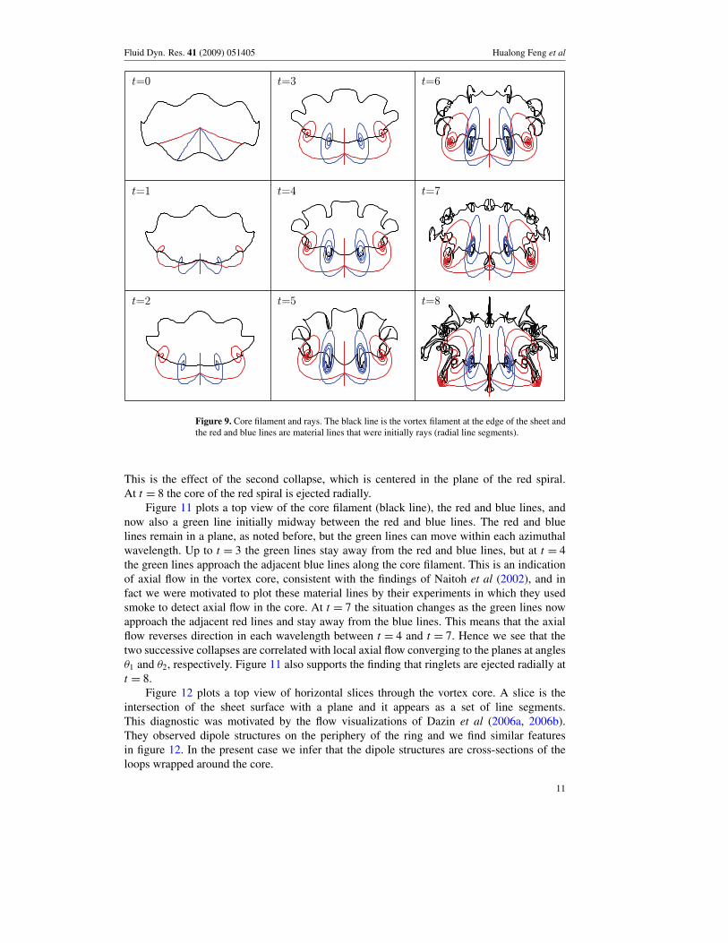
Figure 9 plots a set of material lines. The black line at the edge of the sheet rolls upinto the core and is referred to as the core filament. At t = 0 it has a wavy perturbation. Alsoplotted are red and blue lines that were initially rays (radial line segments). The blue lines areat angles θ1 and the red lines are at angles θ2. The red and blue lines roll up into spirals aroundthe core filament, but they remain in a plane due to the symmetry of the perturbation. At t = 5a hairpin forms in the core filament at angles θ1, corresponding to the first collapse of the core.At this time the core filament is still smooth at angles θ2, but it becomes semi-circular there att = 6 and undergoes severe distortion at t = 7 and t = 8, corresponding to the second collapseof the core. At t = 8 the core of the red spiral is ejected radially.

Figure 10 plots vertical planar cross sections of the sheet containing the red and bluematerial lines. In an axisymmetric problem, the red and blue lines would be identical andindeed they are similar up to t = 2. Thereafter for 2! t ! 6 the outer turn of the blue spiralgrows more rapidly and its core is more distorted, in comparison with the red spiral. This is theeffect of the first collapse, which is centered in the plane of the blue spiral. For 6! t ! 8 thesituation is reversed, as the outer turn of the red spiral grows rapidly and its core is distorted.

10

Fluid Dyn. Res. 41 (2009) 051405 Hualong Feng et al

t=0

t=1

t=2

t=3

t=4

t=5

t=6

t=7

t=8

Figure 9. Core filament and rays. The black line is the vortex filament at the edge of the sheet andthe red and blue lines are material lines that were initially rays (radial line segments).

This is the effect of the second collapse, which is centered in the plane of the red spiral.At t = 8 the core of the red spiral is ejected radially.

Figure 11 plots a top view of the core filament (black line), the red and blue lines, andnow also a green line initially midway between the red and blue lines. The red and bluelines remain in a plane, as noted before, but the green lines can move within each azimuthalwavelength. Up to t = 3 the green lines stay away from the red and blue lines, but at t = 4the green lines approach the adjacent blue lines along the core filament. This is an indicationof axial flow in the vortex core, consistent with the findings of Naitoh et al (2002), and infact we were motivated to plot these material lines by their experiments in which they usedsmoke to detect axial flow in the core. At t = 7 the situation changes as the green lines nowapproach the adjacent red lines and stay away from the blue lines. This means that the axialflow reverses direction in each wavelength between t = 4 and t = 7. Hence we see that thetwo successive collapses are correlated with local axial flow converging to the planes at anglesθ1 and θ2, respectively. Figure 11 also supports the finding that ringlets are ejected radially att = 8.

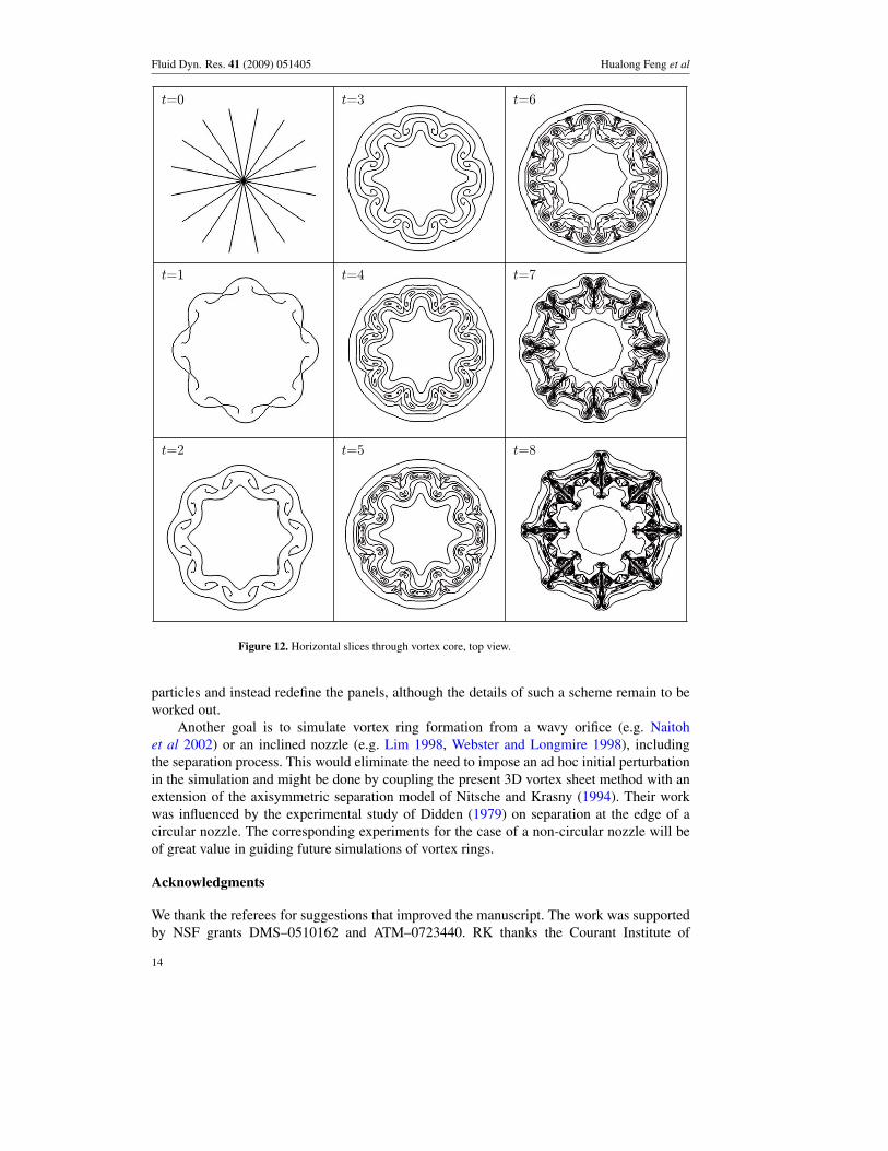
Figure 12 plots a top view of horizontal slices through the vortex core. A slice is theintersection of the sheet surface with a plane and it appears as a set of line segments.This diagnostic was motivated by the flow visualizations of Dazin et al (2006a, 2006b).They observed dipole structures on the periphery of the ring and we find similar featuresin figure 12. In the present case we infer that the dipole structures are cross-sections of theloops wrapped around the core.

11

Fluid Dyn. Res. 41 (2009) 051405 Hualong Feng et al

t=0

t=1

t=2

t=3

t=4

t=5

t=6

t=7

t=8

Figure 10. Planar cross sections through the sheet. The blue line is in the plane of the first collapseand the red line is in the plane of the second collapse.

5. Conclusions

A Lagrangian panel method was presented for vortex sheet roll-up in 3D flow. The methodemploys some common previous techniques such as regularizing the Biot–Savart integraland using a treecode to evaluate the velocity, but it also incorporates some new techniques:(i) representing the sheet by a set of quadrilateral panels having a tree structure, (ii) usingpassive particles to account for panel curvature in the refinement scheme and (iii) evaluatingthe circulation element by equation (12).

Results were presented for the azimuthal instability of a vortex ring starting from aperturbed circular disk vortex sheet initial condition. Details of the core dynamics were

12

Fluid Dyn. Res. 41 (2009) 051405 Hualong Feng et al

t=0

t=1

t=2

t=3

t=4

t=5

t=6

t=7

t=8

Figure 11. Core filament and rays, top view. The black line is the vortex filament at the edge ofthe sheet and the red, blue and green lines are material lines that were initially rays (radial linesegments).

clarified by tracking material lines on the sheet surface. We observed two successive collapsesof the vortex core, out of phase from each other by half an azimuthal wavelength andcorrelated with local axial flow converging to the collapse locations. At late times a sequenceof ringlets is ejected radially from the core. Some features were found to resemble recentexperimental findings on vortex rings, for example by Naitoh et al (2002) on axial flow in thecore of the ring and by Dazin et al (2006a, 2006b) on dipole structures around the peripheryof the ring.

There are several directions for future work. The proposed quadrature scheme amountsto a 2D trapezoid rule and it may be worthwhile to increase the order of accuracy by trackingmore particles on each panel. The panel refinement scheme is effective in resolving the sheet’sroll-up, stretching and folding, but it is not well suited for regions where the sheet is twisting.The twisting is an obstacle to further progress and may require a remeshing scheme. Howeverinstead of resetting the particles to lie on a regular mesh, it may be possible to retain the

13

Fluid Dyn. Res. 41 (2009) 051405 Hualong Feng et al

t=0

t=1

t=2

t=3

t=4

t=5

t=6

t=7

t=8

Figure 12. Horizontal slices through vortex core, top view.

particles and instead redefine the panels, although the details of such a scheme remain to beworked out.

Another goal is to simulate vortex ring formation from a wavy orifice (e.g. Naitohet al 2002) or an inclined nozzle (e.g. Lim 1998, Webster and Longmire 1998), includingthe separation process. This would eliminate the need to impose an ad hoc initial perturbationin the simulation and might be done by coupling the present 3D vortex sheet method with anextension of the axisymmetric separation model of Nitsche and Krasny (1994). Their workwas influenced by the experimental study of Didden (1979) on separation at the edge of acircular nozzle. The corresponding experiments for the case of a non-circular nozzle will beof great value in guiding future simulations of vortex rings.

Acknowledgments

We thank the referees for suggestions that improved the manuscript. The work was supportedby NSF grants DMS–0510162 and ATM–0723440. RK thanks the Courant Institute of

14

Fluid Dyn. Res. 41 (2009) 051405 Hualong Feng et al

Mathematical Sciences for hospitality during the initial preparation of the manuscript andfor support in part by the Applied Mathematical Sciences Program of the US Department ofEnergy under Contract DEFG0200ER25053.

References

Agishtein M E and Migdal A A 1989 Dynamics of vortex surfaces in three dimensions: theory and simulationsPhysica D 40 91–118

Archer P J, Thomas T G and Coleman G N 2008 Direct numerical simulation of vortex ring evolution from thelaminar to the early turbulent regime J. Fluid Mech. 598 201–26

Ashurst W T and Meiburg E 1988 Three-dimensional shear layers via vortex dynamics J. Fluid Mech. 18987–116

Bergdorf M, Koumoutsakos P and Leonard A 2007 Direct numerical simulations of vortex rings at Re' = 7500J. Fluid Mech. 581 495–505

Brady M, Leonard A and Pullin D I 1998 Regularized vortex sheet evolution in three dimensions J. Comput. Phys.146 520–45

Caflisch R E 1988 Mathematical analysis of vortex dynamics Mathematical Aspects of Vortex Dynamics edR E Caflisch (Leesburg, VA: SIAM) pp 1–24

Chorin A J and Bernard P S 1973 Discretization of a vortex sheet with an example of roll-up J. Comput. Phys. 13423–9

Cocle R, Winckelmans G and Daeninck G 2008 Combining the vortex-in-cell and parallel fast multipole methods forefficient domain decomposition simulations J. Comput. Phys. 227 9091–120

Cottet G-H and Koumoutsakos P D 2000 Vortex Methods: Theory and Practice (Cambridge: Cambridge UniversityPress)

Dazin A, Dupont P and Stanislas M 2006a Experimental characterization of the instability of the vortex ring. Part I:Linear phase Exp. Fluids 40 383–99

Dazin A, Dupont P and Stanislas M 2006b Experimental characterization of the instability of the vortex rings. PartII: Non-linear phase Exp. Fluids 41 401–13

Didden N 1979 On the formation of vortex rings: rolling-up and production of circulation Z. Angew. Math. Phys. 30101–16

Feng H 2007 Vortex sheet simulations of 3D flows using an adaptive triangular panel/particle method PhD ThesisUniversity of Michigan

Fukumoto Y and Hattori Y 2005 Curvature instability of a vortex ring J. Fluid Mech. 526 77–115Glezer A and Coles D 1990 An experimental study of a turbulent vortex ring J. Fluid Mech. 211 243–83Johnston H www.math.umass.edu/∼johnston/newtreecode.htmlKaganovskiy L 2006 Hierarchical panel method for vortex sheet motion in three-dimensional flow PhD Thesis

University of MichiganKaganovskiy L 2007 Adaptive panel representation for 3D vortex ring motion and instability Math. Probl. Eng. 68953

doi:10.1155/2007/68953Kaneda Y 1990 A representation of the motion of a vortex sheet in a three-dimensional flow Phys. Fluids A 2 458–61Katz J and Plotkin A 2001 Low-Speed Aerodynamics (Cambridge: Cambridge University Press)Knio O M and Ghoniem A F 1990 Numerical study of a three-dimensional vortex method J. Comput. Phys. 86

75–106Krasny R 1987 Computation of vortex sheet roll-up in the Trefftz plane J. Fluid Mech. 184 123–55Lim T T 1998 On the breakdown of vortex rings from inclined nozzles Phys. Fluids 10 1666–71Lim T T and Nickels T B 1995 Vortex rings Fluid Vortices ed S I Green (Dordrecht: Kluwer) pp 95–153Lindsay K and Krasny R 2001 A particle method and adaptive treecode for vortex sheet motion in three-dimensional

flow J. Comput. Phys. 172 879–907Maxworthy T 1977 Some experimental studies of vortex rings J. Fluid Mech. 81 465–95Moore D W 1972 Finite amplitude waves on aircraft trailing vortices Aeronaut. Q. 23 307–314Moore D W and Saffman P G 1975 The instability of a straight vortex filament in a strain field Proc. R. Soc. Lond. A

346 413–25Naitoh T, Fukuda N, Gotoh T, Yamada H and Nakajima K 2002 Experimental study of axial flow in a vortex ring

Phys. Fluids 14 143–9Nitsche M and Krasny R 1994 A numerical study of vortex ring formation at the edge of a circular tube J. Fluid

Mech. 216 139–61

15

Fluid Dyn. Res. 41 (2009) 051405 Hualong Feng et al

Pozrikidis C 2000 Theoretical and computational aspects of the self-induced motion of three-dimensional vortexsheets J. Fluid Mech. 425 335–66

Rosenhead L 1930 The spread of vorticity in the wake behind a cylinder Proc. R. Soc. Lond. A 127 590–612Saffman P G 1978 The number of waves on unstable vortex rings J. Fluid Mech. 84 625–39Sakajo T 2001 Numerical computation of a three-dimensional vortex sheet in a swirl flow Fluid Dyn. Res. 28 423–48Shariff K and Leonard A 1992 Vortex rings Annu. Rev. Fluid Mech. 24 235–79Shariff K, Verzicco R and Orlandi P 1994 A numerical study of 3-dimensional vortex ring instabilities—viscous

corrections and early nonlinear stage J. Fluid Mech. 279 351–75Stock M J 2006 A regularized inviscid vortex sheet method for three dimensional flows with density interfaces PhD

Thesis University of MichiganStock M J, Dahm W J A and Tryggvason G 2008 Impact of a vortex ring on a density interface using a regularized

inviscid vortex sheet method J. Comput. Phys. 227 9021–43Taylor G I 1953 Formation of a vortex ring by giving an impulse to a circular disc and then dissolving it away J. Appl.

Phys. 24 104–5Webster D R and Longmire E K 1998 Vortex rings from cylinders with inclined exits Phys. Fluids 10 400–16Weigand A and Gharib M 1994 On the decay of a turbulent vortex ring Phys. Fluids 6 3806–8Widnall S E and Tsai C Y 1977 The instability of the thin vortex ring of constant vorticity Phil. Trans. R. Soc. A 287

273–305

16