Axom Documentation

Axom Documentation

LLNL

Feb 11, 2022

Contents

1 Axom Software 3

2 Documentation 5

3 Component Level Dependencies 7

4 Other Tools Application Developers May Find Useful 9

5 Developer Resources 11

6 Communicating with the Axom Team 136.1 Mailing Lists . . . . . . . . . . . . . . . . . . . . . . . . . . . . . . . . . . . . . . . . . . . . . . . 136.2 Chat Room . . . . . . . . . . . . . . . . . . . . . . . . . . . . . . . . . . . . . . . . . . . . . . . . 13

7 Axom Copyright and License Information 157.1 Quickstart Guide . . . . . . . . . . . . . . . . . . . . . . . . . . . . . . . . . . . . . . . . . . . . . 157.2 Axom Core User Guide . . . . . . . . . . . . . . . . . . . . . . . . . . . . . . . . . . . . . . . . . 267.3 Inlet User Guide . . . . . . . . . . . . . . . . . . . . . . . . . . . . . . . . . . . . . . . . . . . . . 417.4 Klee User Guide . . . . . . . . . . . . . . . . . . . . . . . . . . . . . . . . . . . . . . . . . . . . . 607.5 Lumberjack User Guide . . . . . . . . . . . . . . . . . . . . . . . . . . . . . . . . . . . . . . . . . 667.6 Mint User Guide . . . . . . . . . . . . . . . . . . . . . . . . . . . . . . . . . . . . . . . . . . . . . 737.7 Primal User Guide . . . . . . . . . . . . . . . . . . . . . . . . . . . . . . . . . . . . . . . . . . . . 1527.8 Quest User Guide . . . . . . . . . . . . . . . . . . . . . . . . . . . . . . . . . . . . . . . . . . . . 1597.9 Sidre User Guide . . . . . . . . . . . . . . . . . . . . . . . . . . . . . . . . . . . . . . . . . . . . . 1697.10 Slam User Guide . . . . . . . . . . . . . . . . . . . . . . . . . . . . . . . . . . . . . . . . . . . . . 2117.11 Slic User Guide . . . . . . . . . . . . . . . . . . . . . . . . . . . . . . . . . . . . . . . . . . . . . . 2207.12 Spin User Guide . . . . . . . . . . . . . . . . . . . . . . . . . . . . . . . . . . . . . . . . . . . . . 2367.13 Developer Guide . . . . . . . . . . . . . . . . . . . . . . . . . . . . . . . . . . . . . . . . . . . . . 2507.14 Coding Guidelines . . . . . . . . . . . . . . . . . . . . . . . . . . . . . . . . . . . . . . . . . . . . 2817.15 License Info . . . . . . . . . . . . . . . . . . . . . . . . . . . . . . . . . . . . . . . . . . . . . . . 323

i

Axom Documentation

Axom is an open source project that provides robust and flexible software components that serve as building blocksfor high performance scientific computing applications. A key goal of the project is to have different application teamsco-develop and share general core infrastructure software across their projects instead of individually developing andmaintaining capabilities that are similar in functionality but are not easily shared.

An important objective of Axom is to facilitate integration of novel, forward-looking computer science capabilitiesinto simulation codes. A pillar of Axom design is to enable and simplify the exchange of simulation data betweenapplications and tools. Axom developers emphasize the following principles in software design and implementation:

• Start design and implementation based on concrete application use cases and maintain flexibility to meet theneeds of a diverse set of applications

• Develop high-quality, robust, high performance software that has well-designed APIs, good documentation, andsolid testing

• Apply consistent software engineering practices across all Axom components so developers can easily work onthem

• Ensure that components integrate well together and are easy for applications to adopt

The main drivers of Axom capabilities originate in the needs of multiphysics applications in the Advanced Simula-tion and Computing (ASC) Program at Lawrence Livermore National Laboratory (LLNL) . However, Axom can beemployed in a wide range of applications beyond that scope, including research codes, proxy application, etc. Of-ten, developing these types of applications using Axom can facilitate technology transfer from research efforts intoproduction applications.

Contents 1

https://asc.llnl.gov

https://asc.llnl.gov

https://www.llnl.gov

Axom Documentation

2 Contents

CHAPTER 1

Axom Software

Axom software components are maintained and developed on the Axom GitHub Project.

Note: While Axom is developed in C++, its components have native interfaces in C and Fortran for straightforwardusage in applications developed in those languages. Python interfaces are in development.

Our current collection of components is listed here. The number of components and their capabilities will expand overtime as new needs are identified.

• Inlet: Input file parsing and information storage/retrieval

• Klee: Shaping specification and implementation

• Lumberjack: Scalable parallel message logging and filtering

• Mint: Mesh data model

• Primal: Computational geometry primitives

• Quest: Querying on surface tool

• Sidre: Simulation data repository

• Slam: Set-theoretic lightweight API for meshes

• Slic: Simple Logging Interface Code

• Spin: Spatial index structures for managing and accelerating spatial searches

3

https://github.com/LLNL/axom

Axom Documentation

4 Chapter 1. Axom Software

CHAPTER 2

Documentation

User guides and source code documentation are always linked on this site.

• Quickstart Guide

• Source documentation

Core User Guide Source documentationInlet User Guide Source documentationKlee User Guide Source documentationLumberjack User Guide Source documentationMint User Guide Source documentationPrimal User Guide Source documentationQuest User Guide Source documentationSidre User Guide Source documentationSlam User Guide Source documentationSlic User Guide Source documentationSpin User Guide Source documentation

5

doxygen/html/index.html

doxygen/html/coretop.html

doxygen/html/inlettop.html

doxygen/html/kleetop.html

doxygen/html/lumberjacktop.html

doxygen/html/minttop.html

doxygen/html/primaltop.html

doxygen/html/questtop.html

doxygen/html/sidretop.html

doxygen/html/slamtop.html

doxygen/html/slictop.html

doxygen/html/spintop.html

Axom Documentation

6 Chapter 2. Documentation

CHAPTER 3

Component Level Dependencies

Axom has the following inter-component dependencies:

• Core has no dependencies and the other components depend on Core

• Slic optionally depends on Lumberjack

• Slam, Spin, Primal, Mint, Quest, and Sidre depend on Slic

• Mint optionally depends on Sidre

• Inlet depends on Sidre, Slic, and Primal

• Klee depends on Sidre, Slic, Inlet and Primal

• Quest depends on Slam, Spin, Primal, Mint, and, optionally, Klee

The figure below summarizes these dependencies. Solid links indicate hard dependencies; dashed links indicate op-tional dependencies.

7

Axom Documentation

quest

slam primal

mintspin

klee

slic

core

sidre

inlet

lumberjack

8 Chapter 3. Component Level Dependencies

CHAPTER 4

Other Tools Application Developers May Find Useful

The Axom team develops and supports other software tools that are useful for software projects independent of theAxom. These include:

• BLT CMake-based build system developed by the Axom team to simplify CMake usage and development toolintegration

• Shroud Generator for C, Fortran, and Python interfaces to C++ libraries, and Fortran and Python interfaces to Clibraries

• Conduit Library for describing and managing in-memory simulation data

9

https://github.com/LLNL/blt

https://github.com/LLNL/shroud

https://github.com/LLNL/conduit

Axom Documentation

10 Chapter 4. Other Tools Application Developers May Find Useful

CHAPTER 5

Developer Resources

Folks interested in contributing to Axom may be interested in our developer resource guides.

• Developer Guide

• Coding Guide

11

Axom Documentation

12 Chapter 5. Developer Resources

CHAPTER 6

Communicating with the Axom Team

6.1 Mailing Lists

The most effective way to communicate with the Axom team is by using one of our email lists:

• ‘[email protected]’ is for Axom users to contact developers to ask questions, report issues, etc.

• ‘[email protected]’ is mainly for communication among Axom team members

6.2 Chat Room

We also have the ‘Axom’ chat room on the LLNL Microsoft Teams server. This is open to anyone with access to theLLNL network. Just log onto Teams and join the room.

13

mailto:'[email protected]


Axom Documentation

14 Chapter 6. Communicating with the Axom Team

CHAPTER 7

Axom Copyright and License Information

Please see the Axom License.

Copyright (c) 2017-2022, Lawrence Livermore National Security, LLC. Produced at the Lawrence Livermore NationalLaboratory.

LLNL-CODE-741217

7.1 Quickstart Guide

This guide provides information to help Axom users and developers get up and running quickly.

It provides instructions for:

• Obtaining, building and installing third-party libraries on which Axom depends

• Configuring, building and installing the Axom component libraries you want to use

• Compiling and linking an application with Axom

Additional information about Axom can be found on the main Axom Web Page:

• Build system

• User guides and source code documentation for individual Axom components

• Developer guide, coding guidelines, etc.

• Communicating with the Axom development team (email lists, chat room, etc.)

Contents:

7.1.1 Zero to Axom: Quick install of Axom and Third Party Dependencies

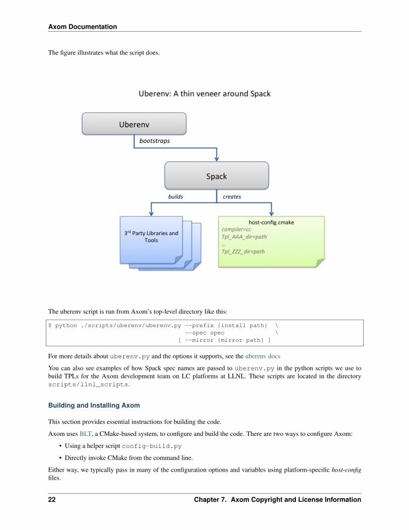
The easiest path to build Axom’s dependencies is to use Spack. This has been encapsulated using Uberenv. Uberenvhelps by doing the following:

15

../../../index.html

https://github.com/spack/spack

https://github.com/LLNL/uberenv

Axom Documentation

• Pulls a blessed version of Spack locally

• If you are on a known operating system, such as the clusters on Livermore Computing (LC), or our provideddocker images, we have defined Spack configuration files to keep Spack from building the world

• Installs our Spack packages into the local Spack

• Simplifies whole dependency build into one command

Uberenv will create a directory containing a Spack instance with the required Axom dependencies installed.

It also generates a host-config file (<config_dependent_name>.cmake) at the root of Axom repository. Thishost-config defines all the required information for building Axom.

$ python3 scripts/uberenv/uberenv.py

Note: On LC machines, it is good practice to do the build step in parallel on a compute node. Here is an examplecommand: salloc -ppdebug -N1-1 python3 scripts/uberenv/uberenv.py

Unless otherwise specified, Spack will default to a compiler. This is generally not a good idea when developing largecodes. To specify which compiler to use, add the compiler specification to the --specUberenv command line option.Supported compiler specs can be found in the Spack compiler files in our repository: scripts/spack/configs/<platform>/compilers.yaml.

We currently regularly test the following Spack configuration files:

• Linux Ubuntu 20.04 (via Windows WSL 2)

• TOSS 3 (On ruby at LC)

• BlueOS (On Lassen at LC)

To install Axom on a new platform, it is a good idea to start with a known Spack configuration directory (located in theAxom repo at scripts/spack/configs/<platform>). The compilers.yaml file describes the compilersand associated flags required for the platform and the packages.yaml file describes the low-level libraries on thesystem to prevent Spack from building the world. Documentation on these configuration files is located in the Spackdocs.

Some helpful uberenv options include :

• --spec=+cuda (build Axom with CUDA support)

• --spec=+devtools (also build the devtools with one command)

• --spec=%[email protected] (build with a specific compiler as defined in the compiler.yaml file)

• --spack-config-dir=<Path to spack configuration directory> (use specific Spackconfiguration files)

• --prefix=<Path> (required, build and install the dependencies in a particular location)

There is more thorough uberenv documentation here.

The modifiers to the Spack specification spec can be chained together, e.g. --spec=%[email protected]+debug+devtools.

If you already have a Spack instance from another project that you would like to reuse, you can do so by changing theuberenv command as follows:

$ python3 scripts/uberenv/uberenv.py --upstream=</path/to/my/spack>/opt/spack

16 Chapter 7. Axom Copyright and License Information

https://spack.readthedocs.io/en/latest/configuration.html

https://spack.readthedocs.io/en/latest/configuration.html

https://uberenv.readthedocs.io/en/latest/

Axom Documentation

Preparing Windows WSL/Ubuntu for Axom installation

For faster installation of the Axom dependencies via Spack on Windows WSL/Ubuntu systems, install CMake,MPICH, openblas, OpenGL, and the various developer tools using the following commands:

Ubuntu 20.04

$ sudo apt-get update$ sudo apt-get upgrade$ sudo apt-get install cmake libopenblas-dev libopenblas-base mpich cppcheck doxygen→˓libreadline-dev python3-sphinx python3-pip clang-format-10 m4$ sudo ln -s /usr/lib/x86_64-linux-gnu/* /usr/lib

Note that the last line is required since Spack expects the system libraries to exist in a directory named lib. Duringthe third party library build phase, the appropriate Spack config directory must be specified using either:

Ubuntu 20.04

python3 scripts/uberenv/uberenv.py --spack-config-dir=scripts/spack/configs/linux_ubuntu_20 --prefix=path/to/install/libraries

Using Axom in Your Project

The install includes examples that demonstrate how to use Axom in CMake-based, BLT-based and Makefile-basedbuild systems.

CMake-based build system example

#------------------------------------------------------------------------------# Check for AXOM_DIR and use CMake's find_package to import axom's targets#------------------------------------------------------------------------------if(NOT DEFINED AXOM_DIR OR NOT EXISTS $AXOM_DIR/lib/cmake/axom-config.cmake)

message(FATAL_ERROR "Missing required 'AXOM_DIR' variable pointing to an→˓installed axom")endif()

find_package(axom REQUIREDNO_DEFAULT_PATHPATHS $AXOM_DIR/lib/cmake)

#------------------------------------------------------------------------------# Set up example target that depends on axom#------------------------------------------------------------------------------add_executable(example example.cpp)

# setup the axom include pathtarget_include_directories(example PRIVATE $AXOM_INCLUDE_DIRS)

# link to axom targetstarget_link_libraries(example axom)target_link_libraries(example fmt)

See: examples/axom/using-with-cmake

7.1. Quickstart Guide 17

Axom Documentation

BLT-based build system example

#------------------------------------------------------------------------------# Set up BLT with validity checks#------------------------------------------------------------------------------

# Check that path to BLT is provided and validif(NOT DEFINED BLT_SOURCE_DIR OR NOT EXISTS $BLT_SOURCE_DIR/SetupBLT.cmake)

message(FATAL_ERROR "Missing required 'BLT_SOURCE_DIR' variable pointing to a→˓valid blt")endif()

include($BLT_SOURCE_DIR/SetupBLT.cmake)

#------------------------------------------------------------------------------# Check for AXOM_DIR and use CMake's find_package to import axom's targets#------------------------------------------------------------------------------if(NOT DEFINED AXOM_DIR OR NOT EXISTS $AXOM_DIR/lib/cmake/axom-config.cmake)

message(FATAL_ERROR "Missing required 'AXOM_DIR' variable pointing to an→˓installed axom")endif()

find_package(axom REQUIREDNO_DEFAULT_PATHPATHS $AXOM_DIR/lib/cmake)

#------------------------------------------------------------------------------# Set up example target that depends on axom#------------------------------------------------------------------------------

blt_add_executable(NAME exampleSOURCES example.cppDEPENDS_ON axom fmt)

See: examples/axom/using-with-blt

Makefile-based build system example

INC_FLAGS=-I$(AXOM_DIR)/include/LINK_FLAGS=-L$(AXOM_DIR)/lib/ -laxom

main:$(CXX) $(INC_FLAGS) example.cpp $(LINK_FLAGS) -o example

See: examples/axom/using-with-make

7.1.2 The Code

Our Git repository contains the Axom source code, documentation, test suites and all files and scripts used for config-uring and building the code. The repository lives in our Github repository.

We use Github for issue tracking. Please report issues, feature requests, etc. there or send email to the Axom develop-ment team.



https://github.com/LLNL/axom/issues

Axom Documentation

Getting the Code

Access to our repository and Atlassian tools requires membership in the LC group axom. If you’re not in the group,please send email to ‘[email protected]’ and request to be added.

SSH keys

If you have not used Github before, you should start by creating and adding your SSH keys to Github. Github providesa good tutorial. Performing these two simple steps will make it easier for you to interact with our Git repositorywithout having to repeatedly enter login credentials.

Cloning the repo

To clone the repo into your local working space, type the following:

$ git clone --recursive [email protected]:LLNL/axom.git

Important notes:

• You don’t need to remember the URL for the Axom repo above. It can be found by going to the Axom repo onour Github project and clicking on the ‘Clone or download’ button that is on the upper right of the Axom Githubpage.

• The --recursive argument above is needed to pull in Axom’s submodules. This includes our data directory,which is used for testing, as well as our build system called BLT, a standalone product that lives in its ownrepository. Documentation for BLT can be found here.

• If you forget to pass the --recursive argument to the git clone command, the following commands can betyped after cloning:

$ cd axom$ git submodule init$ git submodule update

Repository Layout

If you need to look through the repository, this section explains how it is organized. If you do not need this informationand just want to build the code, please continue on to the next section.

The top-level Axom directory contains the following directories:

data The optional axom_data submodule is cloned here.

host-configs Detailed configuration information for platforms and compilers we support.

See Host-config files for more information.

scripts Scripts that we maintain to simplify development and usage tasks

src The bulk of the repo contents.

Within the src directory, you will find the following directories:

axom Directories for individual Axom components (see below)

cmake Axom’s build system lives here.

The BLT submodule is cloned into the blt subdirectory.



https://help.github.com/en/enterprise/2.18/user/github/authenticating-to-github/adding-a-new-ssh-key-to-your-github-account

https://github.com/llnl/blt

https://github.com/llnl/blt

https://llnl-blt.readthedocs.io/en/latest/

Axom Documentation

docs General Axom documentation files

examples Example programs that utilize Axom in their build systems

thirdparty Built-in third party libraries with tests to ensure they are built properly.

In the axom directory, you will find a directory for each of the Axom components. Although there are dependenciesamong them, each is developed and maintained in a largely self-contained fashion. Axom component dependenciesare essentially treated as library dependencies. Each component directory contains subdirectories for the componentheader and implementation files, as well as user documentation, examples and tests.

7.1.3 Configuration and Building

This section provides information about configuring and building the Axom software after you have cloned the repos-itory. The main steps for using Axom are:

1. Configure, build, and install third-party libraries (TPLs) on which Axom depends.

2. Build and install Axom component libraries that you wish to use.

3. Build and link your application with the Axom installation.

Depending on how your team uses Axom, some of these steps, such as installing the Axom TPLs and Axom itself,may need to be done only once. These installations can be shared across the team.

Requirements, Dependencies, and Supported Compilers

Basic requirements:

• C++ Compiler with C++11 support

• CMake

• Fortran Compiler (optional)

Supported Compilers

Axom supports a wide variety of compilers. Please see the <axom_src>/scripts/spack/configs/<platform>/compilers.yaml for an up to date list of the currently supported and tested compilers for eachplatform.

External Dependencies

Axom’s dependencies come in two flavors:

• Library: contain code that axom must link against

• Tool: executables that we use as part of our development process, e.g. to generate documentation and formatour code.

Unless otherwise marked, the dependencies are optional.


Axom Documentation

Library Dependencies

Library Dependent Components Build system variableConduit Required: Sidre CONDUIT_DIRc2c Optional C2C_DIRHDF5 Optional: Sidre HDF5_DIRLua Optional: Inlet LUA_DIRMFEM Optional: Quest MFEM_DIRRAJA Optional: Mint, Spin, Quest RAJA_DIRSCR Optional: Sidre SCR_DIRUmpire Optional: Core, Spin, Quest UMPIRE_DIR

Each library dependency has a corresponding build system variable (with the suffix _DIR) to supply the path to thelibrary’s installation directory. For example, hdf5 has a corresponding variable HDF5_DIR.

Note: Optional c2c library is currently only available for configurations on LLNL clusters.

Tool Dependencies

Tool Purpose Build System Variableclangformat Code Style Checks CLANGFORMAT_EXECUTABLECppCheck Static C/C++ code analysis CPPCHECK_EXECUTABLEDoxygen Source Code Docs DOXYGEN_EXECUTABLELcov Code Coverage Reports LCOV_EXECUTABLEShroud Multi-language binding generation SHROUD_EXECUTABLESphinx User Docs SPHINX_EXECUTABLE

Each tool has a corresponding build system variable (with the suffix _EXECUTABLE) to supply the tool’s executablepath. For example, sphinx has a corresponding build system variable SPHINX_EXECUTABLE.

Note: To get a full list of all dependencies of Axom’s dependencies in an uberenv build of our TPLs, please go tothe TPL root directory and run the following spack command ./spack/bin/spack spec axom.

Building and Installing Third-party Libraries

We use the Spack Package Manager to manage and build TPL dependencies for Axom. The Spack process works onLinux and macOS systems. Axom does not currently have a tool to automatically build dependencies for Windowssystems.

To make the TPL process easier (you don’t really need to learn much about Spack) and automatic, we drive it with apython script called uberenv.py, which is located in the scripts/uberenv directory. Running this script doesseveral things:

• Clones the Spack repo from GitHub and checks out a specific version that we have tested.

• Configures Spack compiler sets, adds custom package build rules and sets any options specific to Axom.

• Invokes Spack to build a complete set of TPLs for each configuration and generates a host-config file thatcaptures all details of the configuration and build dependencies.


https://llnl-conduit.readthedocs.io/en/latest

https://rzlc.llnl.gov/c2c

https://www.hdfgroup.org/solutions/hdf5/

https://www.lua.org/

https://mfem.org/

https://raja.readthedocs.io/en/main/

https://computation.llnl.gov/projects/scalable-checkpoint-restart-for-mpi

https://umpire.readthedocs.io/en/latest/

https://releases.llvm.org/10.0.0/tools/clang/docs/ClangFormat.html

http://cppcheck.sourceforge.net/

http://www.doxygen.nl/

http://ltp.sourceforge.net/coverage/lcov.php

https://shroud.readthedocs.io/en/develop/

http://www.sphinx-doc.org/en/master/

https://github.com/spack/spack

Axom Documentation

The figure illustrates what the script does.

The uberenv script is run from Axom’s top-level directory like this:

$ python ./scripts/uberenv/uberenv.py --prefix install path \--spec spec \

[ --mirror mirror path ]

For more details about uberenv.py and the options it supports, see the uberenv docs

You can also see examples of how Spack spec names are passed to uberenv.py in the python scripts we use tobuild TPLs for the Axom development team on LC platforms at LLNL. These scripts are located in the directoryscripts/llnl_scripts.

Building and Installing Axom

This section provides essential instructions for building the code.

Axom uses BLT, a CMake-based system, to configure and build the code. There are two ways to configure Axom:

• Using a helper script config-build.py

• Directly invoke CMake from the command line.

Either way, we typically pass in many of the configuration options and variables using platform-specific host-configfiles.


https://uberenv.readthedocs.io/en/latest/

https://github.com/LLNL/blt

Axom Documentation

Host-config files

Host-config files help make Axom’s configuration process more automatic and reproducible. A host-config file cap-tures all build configuration information used for the build such as compiler version and options, paths to all TPLs,etc. When passed to CMake, a host-config file initializes the CMake cache with the configuration specified in the file.

We noted in the previous section that the uberenv script generates a host-config file for each item in the Spack spec listgiven to it. These files are generated by spack in the directory where the TPLs were installed. The name of each filecontains information about the platform and spec.

For more information, see BLT’s host-config documentation.

Python helper script

The easiest way to configure the code for compilation is to use the config-build.py python script located inAxom’s base directory; e.g.,:

$ ./config-build.py -hc host-config path

This script requires that you pass it a host-config file. The script runs CMake and passes it the host-config. SeeHost-config files for more information.

Running the script, as in the example above, will create two directories to hold the build and install contents for theplatform and compiler specified in the name of the host-config file.

To build the code and install the header files, libraries, and documentation in the install directory, go into the builddirectory and run make; e.g.,:

$ cd build directory$ make$ make install

Caution: When building on LC systems, please don’t compile on login nodes.

Tip: Most make targets can be run in parallel by supplying the ‘-j’ flag along with the number of threads to use. E.g.$ make -j8 runs make using 8 threads.

The python helper script accepts other arguments that allow you to specify explicitly the build and install paths andbuild type. Following CMake conventions, we support three build types: ‘Release’, ‘RelWithDebInfo’, and ‘Debug’.To see the script options, run the script without any arguments; i.e.,:

$ ./config-build.py

You can also pass extra CMake configuration variables through the script; e.g.,:

$ ./config-build.py -hc host-config file name \-DBUILD_SHARED_LIBS=ON \-DENABLE_FORTRAN=OFF

This will configure cmake to build shared libraries and disable fortran for the generated configuration.


https://llnl-blt.readthedocs.io/en/develop/tutorial/host_configs.html

Axom Documentation

Run CMake directly

You can also configure the code by running CMake directly and passing it the appropriate arguments. For example, toconfigure, build and install a release build with the gcc compiler, you could pass a host-config file to CMake:

$ mkdir build-gcc-release$ cd build-gcc-release$ cmake -C host config file for gcc compiler \

-DCMAKE_BUILD_TYPE=Release \-DCMAKE_INSTALL_PREFIX=../install-gcc-release \../src/

$ make$ make install

Alternatively, you could forego the host-config file entirely and pass all the arguments you need, including paths tothird-party libraries, directly to CMake; for example:

$ mkdir build-gcc-release$ cd build-gcc-release$ cmake -DCMAKE_C_COMPILER=path to gcc compiler \

-DCMAKE_CXX_COMPILER=path to g++ compiler \-DCMAKE_BUILD_TYPE=Release \-DCMAKE_INSTALL_PREFIX=../install-gcc-release \-DCONDUIT_DIR=path/to/conduit/install \many other args \../src/

$ make$ make install

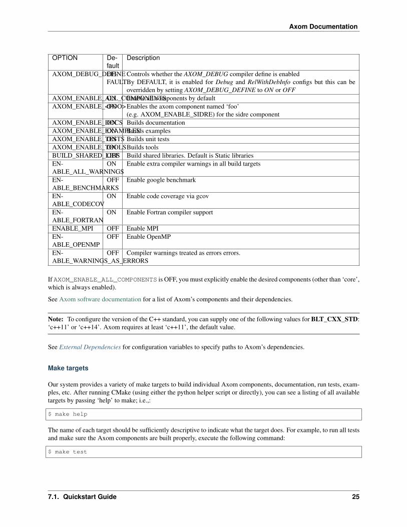
CMake Configuration Options

Here are the key build system options in Axom:


Axom Documentation

OPTION De-fault

Description

AXOM_DEBUG_DEFINEDE-FAULT

Controls whether the AXOM_DEBUG compiler define is enabledBy DEFAULT, it is enabled for Debug and RelWithDebInfo configs but this can beoverridden by setting AXOM_DEBUG_DEFINE to ON or OFF

AXOM_ENABLE_ALL_COMPONENTSON Enable all components by defaultAXOM_ENABLE_<FOO>ON Enables the axom component named ‘foo’

(e.g. AXOM_ENABLE_SIDRE) for the sidre componentAXOM_ENABLE_DOCSON Builds documentationAXOM_ENABLE_EXAMPLESON Builds examplesAXOM_ENABLE_TESTSON Builds unit testsAXOM_ENABLE_TOOLSON Builds toolsBUILD_SHARED_LIBSOFF Build shared libraries. Default is Static librariesEN-ABLE_ALL_WARNINGS

ON Enable extra compiler warnings in all build targets

EN-ABLE_BENCHMARKS

OFF Enable google benchmark

EN-ABLE_CODECOV

ON Enable code coverage via gcov

EN-ABLE_FORTRAN

ON Enable Fortran compiler support

ENABLE_MPI OFF Enable MPIEN-ABLE_OPENMP

OFF Enable OpenMP

EN-ABLE_WARNINGS_AS_ERRORS

OFF Compiler warnings treated as errors errors.

If AXOM_ENABLE_ALL_COMPONENTS is OFF, you must explicitly enable the desired components (other than ‘core’,which is always enabled).

See Axom software documentation for a list of Axom’s components and their dependencies.

Note: To configure the version of the C++ standard, you can supply one of the following values for BLT_CXX_STD:‘c++11’ or ‘c++14’. Axom requires at least ‘c++11’, the default value.

See External Dependencies for configuration variables to specify paths to Axom’s dependencies.

Make targets

Our system provides a variety of make targets to build individual Axom components, documentation, run tests, exam-ples, etc. After running CMake (using either the python helper script or directly), you can see a listing of all availabletargets by passing ‘help’ to make; i.e.,:

$ make help

The name of each target should be sufficiently descriptive to indicate what the target does. For example, to run all testsand make sure the Axom components are built properly, execute the following command:

$ make test


../../../index.html

Axom Documentation

Compiling and Linking with an Application

Please see Preparing Windows WSL/Ubuntu for Axom installation for examples of how to use Axom in your project.

7.2 Axom Core User Guide

The Axom Core component provides fundamental data structures and operations used throughout Axom. Differentcompilers and platforms support these essential building blocks in various ways; the Core library provides a uniforminterface.

Axom Core contains numeric limits and a matrix representation with operators in the axom::numerics namespace.It contains various utilities including a timer class, lexical comparator class, processAbort() function, and nu-meric, filesystem, and string manipulation utilities in the axom::utilities namespace. Axom Core also containsthe axom::Array and axom::StackArray container classes.

Note: The Core library does not depend on any other Axom components/libraries. In particular, Core does not usemacros from the Axom Slic library for output.

7.2.1 API Documentation

Doxygen generated API documentation can be found here: API documentation

Core numerics

The axom::numerics namespace was designed for convenient representation and use of matrices and vectors, withaccompanying manipulation and solver routines.

As an example, the following code shows vector operations.

namespace numerics = axom::numerics;

// First and second vectorsdouble u[] = 4., 1., 0.;double v[] = 1., 2., 3.;double w[] = 0., 0., 0.;

std::cout << "Originally, u and v are" << std::endl<< "u = [" << u[0] << ", " << u[1] << ", " << u[2] << "]" << std::endl<< "v = [" << v[0] << ", " << v[1] << ", " << v[2] << "]"<< std::endl;

// Calculate dot and cross productsdouble dotprod = numerics::dot_product(u, v, 3);numerics::cross_product(u, v, w);

std::cout << "The dot product is " << dotprod << " and the cross product is"<< std::endl<< "[" << w[0] << ", " << w[1] << ", " << w[2] << "]" << std::endl;

// Make u orthogonal to v, then normalize vnumerics::make_orthogonal(u, v, 3);

(continues on next page)


../../../../doxygen/html/coretop.html

Axom Documentation

(continued from previous page)

numerics::normalize(v, 3);

std::cout << "Now orthogonal u and normalized v are" << std::endl<< "u = [" << u[0] << ", " << u[1] << ", " << u[2] << "]" << std::endl<< "v = [" << v[0] << ", " << v[1] << ", " << v[2] << "]"<< std::endl;

// Fill a linear spaceconst int lincount = 45;double s[lincount];numerics::linspace(1., 9., s, lincount);

// Find the real roots of a cubic equation.// (x + 2)(x - 1)(2x - 3) = 0 = 2x^3 - x^2 - 7x + 6 has real roots at// x = -2, x = 1, x = 1.5.double coeff[] = 6., -7., -1., 2.;double roots[3];int numRoots;int result = numerics::solve_cubic(coeff, roots, numRoots);

std::cout << "Root-finding returned " << result<< " (should be 0, success)."

" Found "<< numRoots << " roots (should be 3)" << std::endl<< "at x = " << roots[0] << ", " << roots[1] << ", " << roots[2]<< " (should be x = -2, 1, 1.5 in arbitrary order)." << std::endl;

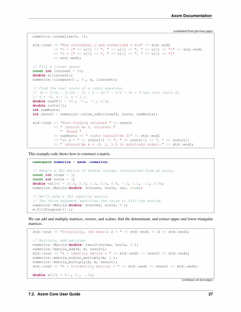
This example code shows how to construct a matrix.

namespace numerics = axom::numerics;

// Here's a 3X3 matrix of double values, initialized from an array.const int nrows = 3;const int ncols = 3;double val[9] = 0.6, 2.4, 1.1, 2.4, 0.6, -.1, 1.1, -.1, 0.6;numerics::Matrix<double> A(nrows, ncols, val, true);

// We'll make a 3X3 identity matrix.// The third argument specifies the value to fill the matrix.numerics::Matrix<double> m(nrows, ncols, 0.);m.fillDiagonal(1.);

We can add and multiply matrices, vectors, and scalars, find the determinant, and extract upper and lower triangularmatrices.

std::cout << "Originally, the matrix A = " << std::endl << A << std::endl;

// Multiply, add matricesnumerics::Matrix<double> result(nrows, ncols, 0.);numerics::matrix_add(A, m, result);std::cout << "A + identity matrix = " << std::endl << result << std::endl;numerics::matrix_scalar_multiply(m, 2.);numerics::matrix_multiply(A, m, result);std::cout << "A * 2*(identity matrix) = " << std::endl << result << std::endl;

double x1[3] = 1., 2., -.5;


7.2. Axom Core User Guide 27

Axom Documentation


double b1[3];std::cout << "Vector x1 = [" << x1[0] << ", " << x1[1] << ", " << x1[2] << "]"

<< std::endl;numerics::matrix_vector_multiply(A, x1, b1);std::cout << "A * x1 = [" << b1[0] << ", " << b1[1] << ", " << b1[2] << "]"

<< std::endl;

// Calculate determinantstd::cout << "Determinant of A = " << numerics::determinant(A) << std::endl;

// Get lower, upper triangle.// By default the diagonal entries are copied from A, but you can get the// identity vector main diagonal entries by passing true as the second// argument.numerics::Matrix<double> ltri = lower_triangular(A);numerics::Matrix<double> utri = upper_triangular(A, true);std::cout << "A's lower triangle = " << std::endl << ltri << std::endl;std::cout << "A's upper triangle (with 1s in the main diagonal) = " << std::endl

<< utri << std::endl;

// Get a column from the matrix.double* col1 = A.getColumn(1);std::cout << "A's column 1 is [" << col1[0] << ", " << col1[1] << ", "

<< col1[2] << "]" << std::endl;

We can also extract rows and columns. The preceding example shows how to get a column. Since the underlyingstorage layout of Matrix is column-based, retrieving a row is a little more involved: the call to getRow() retrieves thestride for accessing row elements p as well the upper bound for element indexes in the row. The next selection showshow to sum the entries in a row.

IndexType p = 0;IndexType N = 0;const T* row = A.getRow(i, p, N);

T row_sum = 0.0;for(IndexType j = 0; j < N; j += p)

row_sum += utilities::abs(row[j]); // END for all columns

We can use the power method or the Jacobi method to find the eigenvalues and vectors of a matrix. The power methodis a stochastic algorithm, computing many matrix-vector multiplications to produce approximations of a matrix’seigenvalues and vectors. The Jacobi method is also an iterative algorithm, but it is not stochastic, and tends to convergemuch more quickly and stably than other methods. However, the Jacobi method is only applicable to symmetricmatrices. In the following snippet, we show both the power method and the Jacobi method to demonstrate that theyget the same answer.

Note: As of August 2020, the API of eigen_solve is not consistent with jacobi_eigensolve(eigen_solve takes a double pointer as input instead of a Matrix and the return codes differ). This is anissue we’re fixing.

// Solve for eigenvectors and values using the power method// The power method calls rand(), so we need to initialize it with srand().std::srand(std::time(0));



Axom Documentation


double eigvec[nrows * ncols];double eigval[nrows];int res = numerics::eigen_solve(A, nrows, eigvec, eigval);std::cout << "Tried to find " << nrows

<< " eigenvectors and values from"" matrix "

<< std::endl<< A << std::endl<< "and the result code was " << res << " (1 = success)."<< std::endl;

if(res > 0)for(int i = 0; i < nrows; ++i)

display_eigs(eigvec, eigval, nrows, i);

// Solve for eigenvectors and values using the Jacobi method.numerics::Matrix<double> evecs(nrows, ncols);res = numerics::jacobi_eigensolve(A, evecs, eigval);std::cout << "Using the Jacobi method, tried to find eigenvectors and "

"eigenvalues of matrix "<< std::endl<< A << std::endl<< "and the result code was " << res << " ("<< numerics::JACOBI_EIGENSOLVE_SUCCESS << " = success)."<< std::endl;

if(res == numerics::JACOBI_EIGENSOLVE_SUCCESS)for(int i = 0; i < nrows; ++i)

display_eigs(evecs, eigval, i);

We can solve a linear system directly or by using LU decomposition and back-substitution.

// Solve a linear system Ax = bnumerics::Matrix<double> A(nrows, ncols);A(0, 0) = 1;A(0, 1) = 2;A(0, 2) = 4;A(1, 0) = 3;A(1, 1) = 8;A(1, 2) = 14;A(2, 0) = 2;A(2, 1) = 6;A(2, 2) = 13;double b[3] = 3., 13., 4.;double x[3];

int rc = numerics::linear_solve(A, b, x);

std::cout << "Solved for x in the linear system Ax = b," << std::endl<< "A = " << std::endl



Axom Documentation


<< A << " and b = [" << b[0] << ", " << b[1] << ", " << b[2]<< "]." << std::endl<< "Result code is " << rc << " (0 = success)" << std::endl;

if(rc == 0)

std::cout << "Found x = [" << x[0] << ", " << x[1] << ", " << x[2] << "]"<< std::endl;

// Solve a linear system Ax = b using LU decomposition and back-substitutionnumerics::Matrix<double> A(nrows, ncols);A(0, 0) = 1;A(0, 1) = 2;A(0, 2) = 4;A(1, 0) = 3;A(1, 1) = 8;A(1, 2) = 14;A(2, 0) = 2;A(2, 1) = 6;A(2, 2) = 13;double b[3] = 3., 13., 4.;double x[3];int pivots[3];

int rc = numerics::lu_decompose(A, pivots);

std::cout << "Decomposed to " << std::endl<< A << " with pivots [" << pivots[0] << ", " << pivots[1] << ", "<< pivots[2] << "]"<< " with result " << rc << " (" << numerics::LU_SUCCESS<< " is success)" << std::endl;

rc = numerics::lu_solve(A, pivots, b, x);if(rc == numerics::LU_SUCCESS)

std::cout << "Found x = [" << x[0] << ", " << x[1] << ", " << x[2] << "]"<< std::endl;

Core utilities

The axom::utilities namespace contains basic commonly-used functions. Often these started out in anotherAxom component and were “promoted” to Axom Core when they were useful in other Axom libraries. In some cases,axom::utilities brings functionality from recent C++ standards to platforms restricted to older compilers.

Axom can print a self-explanatory message and provide a version string.

std::cout << "Here is a message telling you about Axom." << std::endl;axom::about();

std::cout << "The version string '" << axom::getVersion()<< "' is part of the previous message, " << std::endl<< " and is also available separately." << std::endl;


Axom Documentation

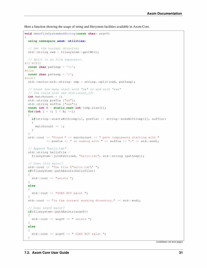
Here a function showing the usage of string and filesystem facilities available in Axom Core.

void demoFileSystemAndString(const char* argv0)

using namespace axom::utilities;

// Get the current directorystd::string cwd = filesystem::getCWD();

// Split it on file separator.#if WIN32

const char pathsep = '\\';#else

const char pathsep = '/';#endif

std::vector<std::string> cmp = string::split(cwd, pathsep);

// Count how many start with "ax" or end with "exe"// (we could also use std::count_if)int matchcount = 0;std::string prefix "ax";std::string suffix "exe";const int N = static_cast<int>(cmp.size());for(int i = 0; i < N; ++i)if(string::startsWith(cmp[i], prefix) || string::endsWith(cmp[i], suffix))

matchcount += 1;

std::cout << "Found " << matchcount << " path components starting with "

<< prefix << " or ending with " << suffix << "." << std::endl;

// Append "hello.txt"std::string hellofile =filesystem::joinPath(cwd, "hello.txt", std::string pathsep);

// Does this exist?std::cout << "The file \"hello.txt\" ";if(filesystem::pathExists(hellofile))std::cout << "exists ";

elsestd::cout << "DOES NOT exist ";

std::cout << "in the current working directory." << std::endl;

// Does argv0 exist?if(filesystem::pathExists(argv0))std::cout << argv0 << " exists ";

elsestd::cout << argv0 << " DOES NOT exist ";



Axom Documentation


std::cout << "in the current working directory." << std::endl;

// sleep for a secondsleep(1);

Axom Core also includes a Timer class. Here, we time the preceding filesystem example snippet.

axom::utilities::Timer t;

t.start();

if(argc == 1)std::cerr << "Error: no path given on command line" << std::endl;return 1;

elsedemoFileSystemAndString(argv[0]);

t.stop();

std::cout << "The tests took " << t.elapsedTimeInMilliSec() << " ms."<< std::endl;

There are several other utility functions. Some are numerical functions such as variations on clamp (ensure a variableis restricted to a given range) and swap (exchange the values of two variables). There are also functions for testingvalues with tolerances, such as isNearlyEqual and isNearlyEqualRelative. These are provided since theywork in device (GPU) kernel code, wheras C++ standard library routines do not. There is also processAbort, togracefully exit an application. For details, please see the Axom Core API Documentation.

Core containers

Warning: Axom’s containers are currently the target of a refactoring effort. The following information is subjectto change, as are the interfaces for the containers themselves. When changes are made to the Axom containers, thechanges will be reflected here.

Axom Core contains the Array, ArrayView, and StackArray classes. Among other things, these data containersfacilitate porting code that uses std::vector to GPUs.

Array

Array is a multidimensional contiguous container template. In the 1-dimensional case, this class behaves similar tostd::vector. In higher dimensions, some vector-like functionality, such as push_back, are not available andmultidimensional-specific operations will mirror the ndarray provided by numpy when possible.

The Array object manages all memory. Typically, the Array object will allocate extra space to facilitate the insertionof new elements and minimize the number of reallocations. The actual capacity of the array (i.e., total number ofelements that the Array can hold) can be queried via the capacity() method. When allocated memory is used


../../../../doxygen/html/coretop.html

Axom Documentation

up, inserting a new element triggers a reallocation. At each reallocation, extra space is allocated according to theresize_ratio parameter, which is set to 2.0 by default. To return all extra memory, an application can call shrink().

Warning: Reallocations tend to be costly operations in terms of performance. Use reserve()when the numberof nodes is known a priori, or use a constructor that takes an actual size and capacity when possible.

Note: The Array destructor deallocates and returns all memory associated with it to the system.

Here’s an example showing how to use Array instead of std::vector.

// Here is an Array of ints with length three.axom::Array<int> a(3);std::cout << "Length of a = " << a.size() << std::endl;a[0] = 2;a[1] = 5;a[2] = 11;

// An Array increases in size if a value is pushed back.a.push_back(4);std::cout << "After pushing back a value, a's length = " << a.size()

<< std::endl;

// You can also insert a value in the middle of the Array.// Here we insert value 6 at position 2 and value 1 at position 4.showArray(a, "a");a.insert(2, 6);a.insert(4, 1);std::cout << "After inserting two values, ";showArray(a, "a");

The output of this example is:

Length of a = 3After appending a value, a's length = 4Array a = [2, 5, 11, 4]After inserting two values, Array a = [2, 5, 6, 11, 1, 4]

Applications commonly store tuples of data in a flat array or a std::vector. In this sense, it can be thought ofas a two-dimensional array. Array supports arbitrary dimensionalities but an alias, MCArray (or Multi-ComponentArray), is provided for this two-dimensional case.

The MCArray (i.e., Array<T, 2>) class formalizes tuple storage, as shown in the next example.

// Here is an MCArray of ints, containing two triples.const int numTuples = 2;const int numComponents = 3;axom::MCArray<int> b(numTuples, numComponents);// Set tuple 0 to (1, 4, 2).b(0, 0) = 1;b(0, 1) = 4;b(0, 2) = 2;// Set tuple 1 to one tuple, (8, 0, -1).// The first argument to set() is the buffer to copy into the MCArray, the// second is the number of tuples in the buffer, and the third argument



Axom Documentation


// is the first tuple to fill from the buffer.int ival[3] = 8, 0, -1;b.set(ival, 3, 3);

showTupleArray(b, "b");

// Now, insert two tuples, (0, -1, 1), (1, -1, 0), into the MCArray, directly// after tuple 0.int jval[6] = 0, -1, 1, 1, -1, 0;b.insert(1, numTuples * numComponents, jval);

showTupleArray(b, "b");


MCArray b with 2 3-tuples = [[1, 4, 2][8, 0, -1]

]MCArray b with 4 3-tuples = [

[1, 4, 2][0, -1, 1][1, -1, 0][8, 0, -1]

]

ArrayView

It is also often useful to wrap an external, user-supplied buffer without taking ownership of the data. For this purposeAxom provides the ArrayView class, which is a lightweight wrapper over a buffer that provides one- or multi-dimensional indexing/reshaping semantics. For example, it might be useful to reinterpret a flat (one-dimensional)array as a two-dimensional array. This is accomplished via MCArrayView which, similar to the MCArray alias, isan alias for ArrayView<T, 2>.

// The internal buffer maintained by an MCArray is accessible.int* pa = a.data();// An MCArray can be constructed with a pointer to an external buffer.// Here's an Array interpreting the memory pointed to by pa as three 2-tuples.axom::MCArrayView<int> c(pa, 3, 2);

showArray(a, "a");showTupleArrayView(c, "c");

// Since c is an alias to a's internal memory, changes affect both Arrays.a[0] = 1;c(1, 1) = 9;

std::cout<< "Array a and MCArrayView c use the same memory, a's internal buffer."<< std::endl;

showArray(a, "a");showTupleArrayView(c, "c");



Axom Documentation

Array a = [2, 5, 6, 11, 1, 4]MCArrayView c with 3 2-tuples = [[2, 5][6, 11][1, 4]

]Array a and MCArrayView c use the same memory, a's internal buffer.Array a = [1, 5, 6, 9, 1, 4]MCArrayView c with 3 2-tuples = [[1, 5][6, 9][1, 4]

]

Note: The set of permissible operations on an ArrayView is somewhat limited, as operations that would cause thebuffer to resize are not permitted.

In the future, it will also be possible to restride an ArrayView.

Iteration is also identical between the Array and ArrayView classes. In particular:

• operator() indexes into multidimensional data. Currently, the number of indexes passed must match thedimensionality of the array.

• operator[] indexes into the full buffer, i.e., arr[i] is equivalent to arr.data()[i].

• begin() and end() refer to the full buffer.

Consider the following example:

// Iteration over multidimensional arrays uses the shape() method// to retrieve the extents in each dimension.for(int i = 0; i < c.shape()[0]; i++)for(int j = 0; j < c.shape()[1]; j++)

// Note that c's operator() accepts two arguments because it is two-dimensionalstd::cout << "In ArrayView c, index (" << i << ", " << j << ") yields "

<< c(i, j) << std::endl;

// To iterate over the "flat" data in an Array, regardless of dimension,// use a range-based for loop.std::cout << "Range-based for loop over ArrayView c yields: ";for(const int value : c)std::cout << value << " ";

std::cout << std::endl;

// Alternatively, the "flat" data can be iterated over with operator[]// from 0 -> size().std::cout << "Standard for loop over ArrayView c yields: ";for(int i = 0; i < c.size(); i++)std::cout << c[i] << " ";



Axom Documentation




In ArrayView c, index (0, 0) yields 1In ArrayView c, index (0, 1) yields 5In ArrayView c, index (1, 0) yields 6In ArrayView c, index (1, 1) yields 9In ArrayView c, index (2, 0) yields 1In ArrayView c, index (2, 1) yields 4Range-based for loop over ArrayView c yields: 1 5 6 9 1 4Standard for loop over ArrayView c yields: 1 5 6 9 1 4

Using Arrays in GPU Code

Instead of writing kernels and device functions that operate on raw pointers, we can use ArrayView in device code.The basic “workflow” for this process is as follows:

1. Create an Array allocated in device-accessible memory via either specifying an allocator ID or using a classtemplate parameter for the desired memory space.

2. Write a kernel that accepts an ArrayView parameter by value, not by reference or pointer.

3. Create an ArrayView from the Array to call the function. For non-templated kernels an implicit conversionis provided.

The full template signature for Array (ArrayView has an analogous signature) is Array<typename T, intDIM = 1, MemorySpace SPACE = MemorySpace::Dynamic>. Of particular interest is the last parame-ter, which specifies the memory space in which the array’s data are allocated. The default, Dynamic, means that thememory space is set via an allocator ID at runtime.

Note: Allocating Array s in different memory spaces is only possible when Umpire is available. To learn moreabout Umpire, see the Umpire documentation

Setting the MemorySpace to an option other than Dynamic (for example, MemorySpace::Device) provides acompile-time guarantee that data can always be accessed from a GPU. “Locking down” the memory space at compiletime can help to prevent illegal memory accesses and segmentation faults when pointers are dereferenced from thewrong execution space.

To summarize, there are a couple different options for creating an ArrayView. Consider a function that takes as anargument an ArrayView on the device:

void takesDeviceArrayView(axom::ArrayView<int, 1, axom::MemorySpace::Device>)

To create an argument to this function we can select the space either at runtime or at compile-time as follows:

constexpr int N = 10;// An device array can be constructed by either specifying the corresponding

→˓allocator ID...const int device_allocator_id = axom::getUmpireResourceAllocatorID(umpire::resource::MemoryResourceType::Device);

axom::Array<int> device_array_dynamic(N, N, device_allocator_id);// ...or by providing the memory space via template parameter:axom::Array<int, 1, axom::MemorySpace::Device> device_array_template(N);


https://readthedocs.org/projects/umpire

Axom Documentation

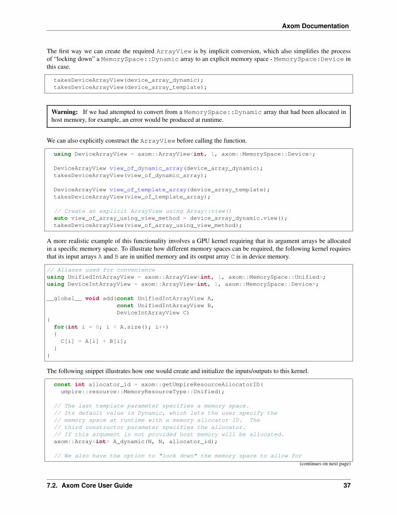
The first way we can create the required ArrayView is by implicit conversion, which also simplifies the processof “locking down” a MemorySpace::Dynamic array to an explicit memory space - MemorySpace:Device inthis case.

takesDeviceArrayView(device_array_dynamic);takesDeviceArrayView(device_array_template);

Warning: If we had attempted to convert from a MemorySpace::Dynamic array that had been allocated inhost memory, for example, an error would be produced at runtime.

We can also explicitly construct the ArrayView before calling the function.

using DeviceArrayView = axom::ArrayView<int, 1, axom::MemorySpace::Device>;

DeviceArrayView view_of_dynamic_array(device_array_dynamic);takesDeviceArrayView(view_of_dynamic_array);

DeviceArrayView view_of_template_array(device_array_template);takesDeviceArrayView(view_of_template_array);

// Create an explicit ArrayView using Array::view()auto view_of_array_using_view_method = device_array_dynamic.view();takesDeviceArrayView(view_of_array_using_view_method);

A more realistic example of this functionality involves a GPU kernel requiring that its argument arrays be allocatedin a specific memory space. To illustrate how different memory spaces can be required, the following kernel requiresthat its input arrays A and B are in unified memory and its output array C is in device memory.

// Aliases used for convenienceusing UnifiedIntArrayView = axom::ArrayView<int, 1, axom::MemorySpace::Unified>;using DeviceIntArrayView = axom::ArrayView<int, 1, axom::MemorySpace::Device>;

__global__ void add(const UnifiedIntArrayView A,const UnifiedIntArrayView B,DeviceIntArrayView C)

for(int i = 0; i < A.size(); i++)C[i] = A[i] + B[i];

The following snippet illustrates how one would create and initialize the inputs/outputs to this kernel.

const int allocator_id = axom::getUmpireResourceAllocatorID(umpire::resource::MemoryResourceType::Unified);

// The last template parameter specifies a memory space.// Its default value is Dynamic, which lets the user specify the// memory space at runtime with a memory allocator ID. The// third constructor parameter specifies the allocator.// If this argument is not provided host memory will be allocated.axom::Array<int> A_dynamic(N, N, allocator_id);

// We also have the option to "lock down" the memory space to allow for



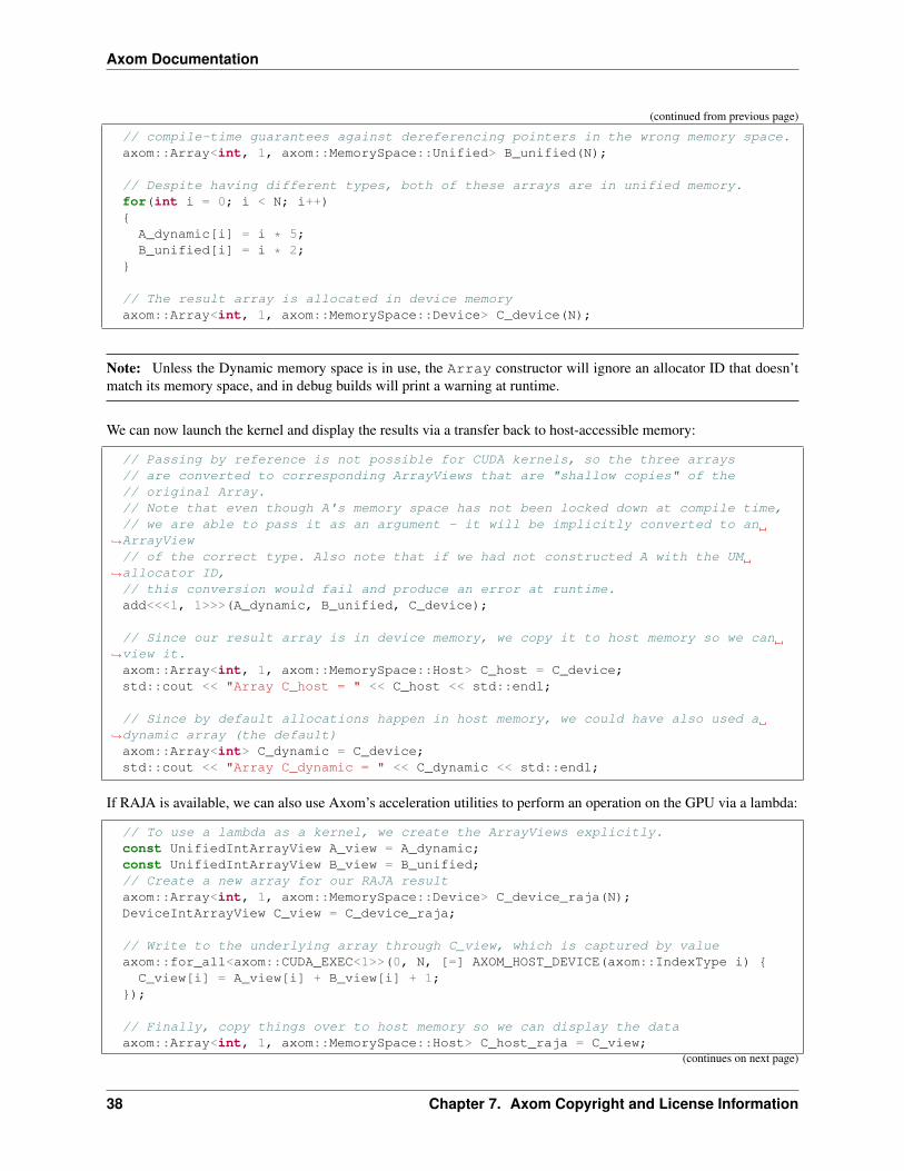
Axom Documentation


// compile-time guarantees against dereferencing pointers in the wrong memory space.axom::Array<int, 1, axom::MemorySpace::Unified> B_unified(N);

// Despite having different types, both of these arrays are in unified memory.for(int i = 0; i < N; i++)A_dynamic[i] = i * 5;B_unified[i] = i * 2;

// The result array is allocated in device memoryaxom::Array<int, 1, axom::MemorySpace::Device> C_device(N);

Note: Unless the Dynamic memory space is in use, the Array constructor will ignore an allocator ID that doesn’tmatch its memory space, and in debug builds will print a warning at runtime.

We can now launch the kernel and display the results via a transfer back to host-accessible memory:

// Passing by reference is not possible for CUDA kernels, so the three arrays// are converted to corresponding ArrayViews that are "shallow copies" of the// original Array.// Note that even though A's memory space has not been locked down at compile time,// we are able to pass it as an argument - it will be implicitly converted to an

→˓ArrayView// of the correct type. Also note that if we had not constructed A with the UM

→˓allocator ID,// this conversion would fail and produce an error at runtime.add<<<1, 1>>>(A_dynamic, B_unified, C_device);

// Since our result array is in device memory, we copy it to host memory so we can→˓view it.axom::Array<int, 1, axom::MemorySpace::Host> C_host = C_device;std::cout << "Array C_host = " << C_host << std::endl;

// Since by default allocations happen in host memory, we could have also used a→˓dynamic array (the default)axom::Array<int> C_dynamic = C_device;std::cout << "Array C_dynamic = " << C_dynamic << std::endl;

If RAJA is available, we can also use Axom’s acceleration utilities to perform an operation on the GPU via a lambda:

// To use a lambda as a kernel, we create the ArrayViews explicitly.const UnifiedIntArrayView A_view = A_dynamic;const UnifiedIntArrayView B_view = B_unified;// Create a new array for our RAJA resultaxom::Array<int, 1, axom::MemorySpace::Device> C_device_raja(N);DeviceIntArrayView C_view = C_device_raja;

// Write to the underlying array through C_view, which is captured by valueaxom::for_all<axom::CUDA_EXEC<1>>(0, N, [=] AXOM_HOST_DEVICE(axom::IndexType i) C_view[i] = A_view[i] + B_view[i] + 1;

);

// Finally, copy things over to host memory so we can display the dataaxom::Array<int, 1, axom::MemorySpace::Host> C_host_raja = C_view;



Axom Documentation


std::cout << "Array C_host_raja = " << C_host_raja << std::endl;

StackArray

The StackArray class is a work-around for a limitation in older versions of the nvcc compiler, which do not capturearrays on the stack in device lambdas. More details are in the API documentation and in the tests.

Core acceleration

Axom’s core component provides several utilities for user applications that intend to support execution on hardwareaccelerators. Axom lets users control execution space using RAJA and memory space using Umpire. As noted in theRAJA documentation, developers of high-performance computing applications have many options for running code:on the CPU, using OpenMP, or on GPU hardware accelerators, and the options are constantly developing. RAJAcontrols where code runs; Umpire moves data between memory spaces.

Note: Axom’s memory management and execution space APIs have default implementations when Axom is notconfigured with Umpire and RAJA, respectively, and can be used in all Axom configurations.

The memory management API allows the user to leverage either C++ memory functions or Umpire, depending on theavailability of Umpire at compilation. It supports a simple operation set: allocate, deallocate, reallocate, and copy. IfUmpire is in use, an allocator can be specified – see Umpire documentation for more details. Note that the fall-backto C++ memory functions is automatic, so the same piece of code can handle standard C++ or C++ with Umpire.However, to use advanced features, such as accessing unified memory, Umpire must be enabled, otherwise errors willoccur at compilation.

Here is an example of using Axom’s memory management tools:

int *dynamic_memory_array;int *dyn_array_dst;int len = 20;

//Allocation looks similar to use of malloc() in C -- just template//return type instead of casting.dynamic_memory_array = axom::allocate<int>(len);

for(int i = 0; i < len; i++)dynamic_memory_array[i] = i;

for(int i = 0; i < len; i++)std::cout << i << " Current value: " << dynamic_memory_array[i] << std::endl;

dyn_array_dst = axom::allocate<int>(len);

//Now, a copy operation. It's used exactly like memcpy -- destination, source,→˓number of bytes.axom::copy(dyn_array_dst, dynamic_memory_array, sizeof(int) * len);

for(int i = 0; i < len; i++)(continues on next page)


https://raja.readthedocs.io/en/main/index.html

https://readthedocs.org/projects/umpire

Axom Documentation


std::cout << i << " Current value: " << dyn_array_dst[i] << std::endl;std::cout << "Matches old value? " << std::boolalpha

<< (dynamic_memory_array[i] == dyn_array_dst[i]) << std::endl;

//Deallocate is exactly like free. Of course, we won't try to access the now-→˓deallocated//memory after this:axom::deallocate(dyn_array_dst);

//Reallocate is like realloc -- copies existing contents into a larger memory space.//Slight deviation from realloc() in that it asks for item count, rather than bytes.dynamic_memory_array = axom::reallocate(dynamic_memory_array, len * 2);for(int i = 20; i < len * 2; i++)dynamic_memory_array[i] = i;

for(int i = 0; i < len * 2; i++)std::cout << i << " Current value: " << dynamic_memory_array[i] << std::endl;

Throughout Axom, acceleration is increasingly supported. Both internally, and to support users, Axom Core offers aninterface that, using RAJA and Umpire internally, provides easy access to for-loop level acceleration via the parallel-foridiom, which applies a given lambda function for every index in range.

Here is an Axom example showing sequential execution:

//This part of the code works regardless of Umpire's presence, allowing for generic//use of axom::allocate in C++ code.int *A = axom::allocate<int>(N);int *B = axom::allocate<int>(N);int *C = axom::allocate<int>(N);

for(int i = 0; i < N; i++)A[i] = i * 5;B[i] = i * 2;C[i] = 0;

//Axom provides an API for the most basic usage of RAJA, the for_all loop.axom::for_all<axom::SEQ_EXEC>(0,N,AXOM_LAMBDA(axom::IndexType i) C[i] = A[i] + B[i]; );

std::cout << "Sums: " << std::endl;for(int i = 0; i < N; i++)std::cout << C[i] << " ";C[i] = 0;

Here’s the same loop from the above snippet, this time with CUDA:


Axom Documentation

//This example requires Umpire to be in use, and Unified memory available.const int allocator_id = axom::getUmpireResourceAllocatorID(umpire::resource::MemoryResourceType::Unified);

A = axom::allocate<int>(N, allocator_id);B = axom::allocate<int>(N, allocator_id);C = axom::allocate<int>(N, allocator_id);

for(int i = 0; i < N; i++)A[i] = i * 5;B[i] = i * 2;C[i] = 0;

axom::for_all<axom::CUDA_EXEC<256>>(0,N,AXOM_LAMBDA(axom::IndexType i) C[i] = A[i] + B[i]; );

std::cout << "Sums: " << std::endl;for(int i = 0; i < N; i++)std::cout << C[i] << " ";


For more advanced functionality, users can directly call RAJA and Umpire. See the RAJA documentation and theUmpire documentation.

7.3 Inlet User Guide

Note: Inlet, and this guide, is under heavy development.

Inlet, named because it provides a place of entry, is a C++ library that provides an easy way to read, store, and accessinput files for computer simulations in a variety of input languages.



7.3.2 Introduction

Inlet provides an easy and extensible way to handle input files for a simulation code. We provide readers for JSON,Lua, and YAML. Additional languages can be supported via an implementation of Inlet’s Reader interface.

All information read from the input file is stored via Inlet into a user-provided Sidre DataStore. This allows us toutilize the functionality of Sidre, such as simulation restart capabilities.

Inlet is used to define the schema of the information expected in your input file. That data is then read via a Readerclass into the Sidre Datastore. You can then verify that the input file met your criteria and use that information later inyour code.

7.3. Inlet User Guide 41

https://raja.readthedocs.io

https://umpire.readthedocs.io

../../../../doxygen/html/inlettop.html

Axom Documentation

7.3.3 Requirements

• Sidre - Inlet stores all data from the input file in the Sidre DataStore

• (Optional) Lua - Inlet provides a Lua reader class that assists in Lua input files

7.3.4 Glossary

• inlet::Container: Internal nodes of the Inlet hierarchy

• inlet::Field: Terminal nodes of the Inlet hierarchy that store primitive types (bool, int, string, double)

• inlet::Function: Terminal nodes of the Inlet hierarchy that store function callbacks

• inlet::Proxy: Provides type-erased access to data in the Inlet hierarchy - can refer to either a Container,Field, or Function internally

• struct: Refers to something that maps to a C++ struct. This can be a Lua table, a YAML dictionary, or aJSON object.

• dictionary: Refers to an associative array whose keys are either strings or a mix of strings and integers, andwhose values are of homogeneous type

• array: Refers to either a contiguous array or an integer-keyed associative array whose values are of homoge-neous type

• collection: Refers to either an array or dictionary

Quick Start

Inlet’s workflow is broken into the four following steps:

• Defining the schema of your input file and reading in the user-provided input file

• Verifying that the user-provided input file is valid

• Accessing the input data in your program

• Optional Generating documentation based on defined schema

Defining Schema

The first step in using Inlet is to define the schema of your input file. Inlet defines an input file into two basic classes:Containers and Fields. Basically Fields are individual values and Containers hold groups of Fields and Containers.

Define the schema by using the following functions, on either the main Inlet class, for global Containers and Fields,or on individual Container instances, for Containers and Fields under that Container:

Name DescriptionaddContainer Adds a Container to the input file schema with the given name.addBool Adds a boolean Field to the global or parent Container with the given name.addDouble Adds a double Field to the global or parent Container with the given name.addInt Adds a integer Field to the global or parent Container with the given name.addString Adds a string Field to the global or parent Container with the given name.

All possible Containers and Fields that are can be found in the input file must be defined at this step. The value of theField is read and stored into the Sidre datastore when you call the appropriate add function. Use the required class


Axom Documentation

member function on the Container and Field class to indicate that they have to present in the given input file. You canalso set a default value to each field via the type-safe Field::defaultValue() member functions. Doing so willpopulate the corresponding Fields value if the specific Field is not present in the input file. The following exampleshows these concepts:

// defines a required global field named "dimensions" with a default value of 2myInlet.addInt("dimensions").required(true).defaultValue(2);

// _inlet_verification_container_start// defines a required container named vector with an internal field named 'x'auto& v = myInlet.addStruct("vector").required(true);// _inlet_verification_container_endv.addDouble("x");

Verification

This step helps ensure that the given input file follows the rules expected by the code. This should be done aftercompletely defining your schema, which also reads in the values in the input file. This allows you to access any otherpart of the user-provided input. These rules are not verified until you call Inlet::verify(). Doing so will returntrue/false and output SLIC warnings to indicate which Field or Container violated which rule.

As shown above, both Containers and Fields can be marked as required. Fields have two additional basic rules thatcan be enforced with the following Field class member functions:

Name DescriptionvalidValues Indicates the Field can only be set to one of the given values.range Indicates the Field can only be set to inclusively between two values.

Inlet also provides functionality to write your own custom rules via callable lambda verifiers. Fields and Containerscan both register one lambda each via their registerVerifier() member functions. The following exampleadds a custom verifier that simply verifies that the given dimensions field match the length the given vector:

v.registerVerifier([&myInlet](const axom::inlet::Container& container) -> bool int dim = myInlet["dimensions"];bool x_present = container.contains("x") &&

(container["x"].type() == axom::inlet::InletType::Double);bool y_present = container.contains("y") &&

(container["y"].type() == axom::inlet::InletType::Double);bool z_present = container.contains("z") &&

(container["z"].type() == axom::inlet::InletType::Double);if(dim == 1 && x_present)

return true;else if(dim == 2 && x_present && y_present)

return true;else if(dim == 3 && x_present && y_present && z_present)

return true;return false;

);



Axom Documentation


std::string msg;// We expect verification to be unsuccessful since the only Field// in vector is x but 2 dimensions are expectedSLIC_INFO("This should fail due to a missing dimension:");myInlet.verify() ? msg = "Verification was successful\n"

: msg = "Verification was unsuccessful\n";SLIC_INFO(msg);

// Add required dimension to schemav.addDouble("y");

// We expect the verification to succeed because vector now contains// both x and y to match the 2 dimensionsSLIC_INFO("After adding the required dimension:");myInlet.verify() ? msg = "Verification was successful\n"

: msg = "Verification was unsuccessful\n";SLIC_INFO(msg);

Note: Inlet::getGlobalContainer()->registerVerifier() can be used to add a verifier to applyrules to the Fields at the global level.

For a full description of Inlet’s verification rules, see Verification.

Accessing Data

After the input file has been read and verified by the previous steps, you can access the data by name viaInlet::get() functions. These functions are type-safe, fill the given variable with what is found, and return aboolean whether the Field was present in the input file or had a default value it could fall back on. Variables, on theInlet side, are used in a language-agnostic way and are then converted to the language-specific version inside of theappropriate Reader. For example, Inlet refers to the Lua variable vector=x=3 or vector.x as vector/xon all Inlet function calls.

For example, given the previous verificiation example, this access previously read values:

// Get dimensions if it was present in input fileauto proxy = myInlet["dimensions"];if(proxy.type() == axom::inlet::InletType::Integer)msg = "Dimensions = " + std::to_string(proxy.get<int>()) + "\n";SLIC_INFO(msg);

// Get vector information if it was present in input filebool x_found = myInlet["vector/x"].type() == axom::inlet::InletType::Double;bool y_found = myInlet["vector/y"].type() == axom::inlet::InletType::Double;if(x_found && y_found)msg = "Vector = " + std::to_string(myInlet["vector/x"].get<double>()) +

"," + std::to_string(myInlet["vector/y"].get<double>()) + "\n";SLIC_INFO(msg);


Axom Documentation

Generating Documentation

We provide a slightly more complex but closer to a real world Inlet usage example of the usage of Inlet. You can findthat example in our repository here.

Once you have defined your schema, call write() on your Inlet class, passing it a concrete instantiation of aWriter class.

inlet.write(SphinxWriter("example_doc.rst"));

We provided a basic Sphinx documentation writing class but you may want to customize it to your own style. Thelinks below show the example output from the documentation_generation.cpp, mfem_coefficient.cpp, and nested_structs.cpp examples:

Example Output: Input file Options

thermal_solver

Table 7.1: FieldsField Name Description Default Value Range/Valid Val-

uesRequired

timestepper thermal solvertimestepper

quasistatic quasistatic, for-wardeuler, back-wardeuler

order polynomial order 1 to 2147483647

solver


uesRequired

dt time step 1.000000 0.000e+00 to1.798e+308

steps number ofsteps/cycles totake

1 1 to 2147483647

print_level solver print/debuglevel

0 0 to 3

rel_tol solver relative toler-ance

0.000001 0.000e+00 to1.798e+308

max_iter maximum iterationlimit

100 1 to 2147483647

abs_tol solver absolute tol-erance

0.000000 0.000e+00 to1.798e+308


https://github.com/LLNL/axom/blob/develop/src/axom/inlet/examples/document_generation.cpp

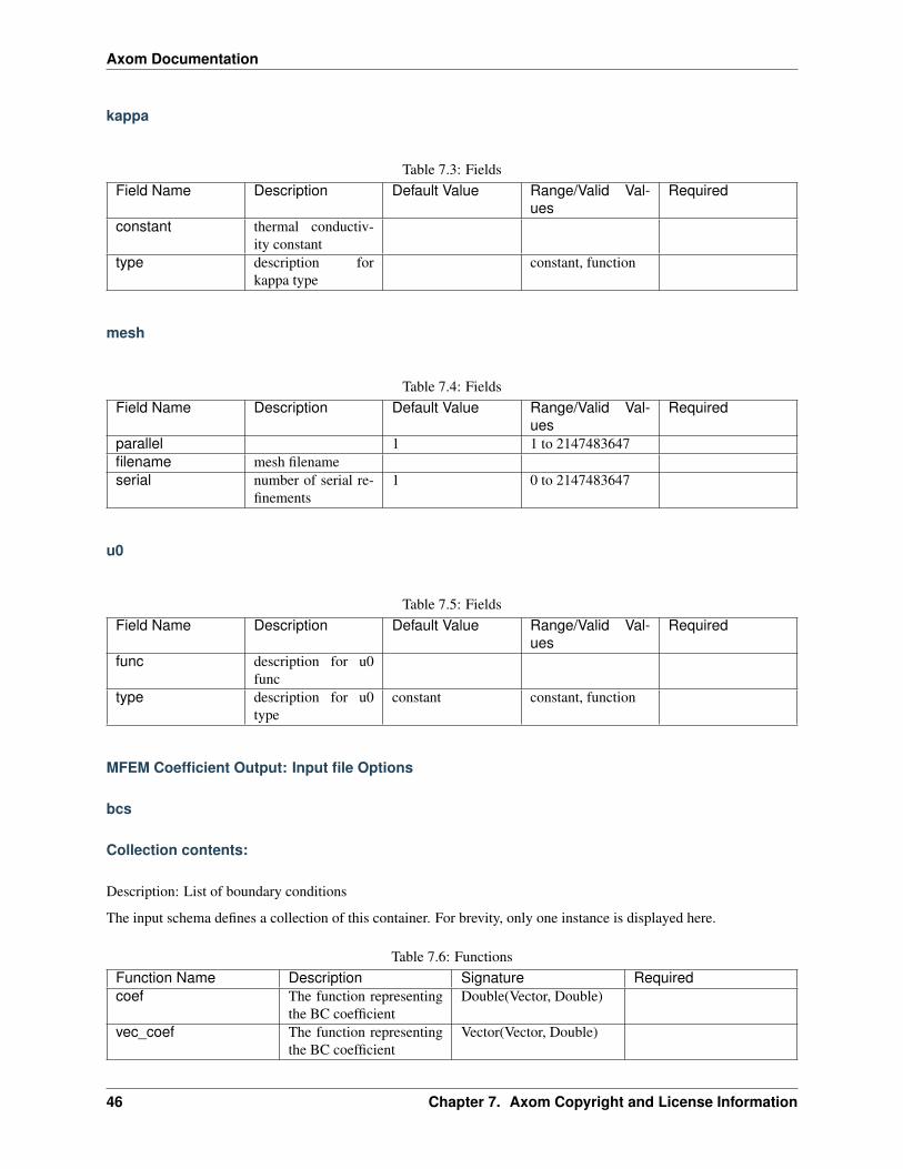
Axom Documentation

kappa


uesRequired

constant thermal conductiv-ity constant

type description forkappa type

constant, function

mesh


uesRequired

parallel 1 1 to 2147483647filename mesh filenameserial number of serial re-

finements1 0 to 2147483647

u0


uesRequired

func description for u0func

type description for u0type

constant constant, function

MFEM Coefficient Output: Input file Options

bcs

Collection contents:

Description: List of boundary conditions

The input schema defines a collection of this container. For brevity, only one instance is displayed here.

Table 7.6: FunctionsFunction Name Description Signature Requiredcoef The function representing

the BC coefficientDouble(Vector, Double)

vec_coef The function representingthe BC coefficient

Vector(Vector, Double)


Axom Documentation

attrs


Description: List of boundary attributes


uesRequired

123

Nested Structs Output: Input file Options

shapes




uesRequired

material Material of theshape

steel, wood, plastic

name Name of the shape

geometry

Description: Geometric information on the shape


uesRequired

start_dimensions Dimension in whichto begin applyingoperations

3

units Units for length cm cm, mpath Path to the shape fileformat File format for the

shape

operators


Axom Documentation


Description: List of shape operations to apply



uesRequired

rotate Degrees of rotation -1.800e+02 to1.800e+02

slice

Description: Options for a slice operation


uesRequired

z z-axis point to sliceon

y y-axis point to sliceon

x x-axis point to sliceon

translate


Description: Translation vector


uesRequired

012

Inlet also provides a utility for generating a JSON schema from your input file schema. This allows for integration withtext editors like Visual Studio Code, which allows you to associate a JSON schema with an input file and subsequentlyprovides autocompletion, linting, tooltips, and more. VSCode and other editors currently support verification of JSONand YAML input files with JSON schemas.

Using the same documentation_generation.cpp example, the automatically generated schema can be usedto assist with input file writing:


https://json-schema.org/

Axom Documentation

Readers

Inlet has built-in support for three input file languages: JSON, Lua, and YAML. Due to language features, not allreaders support all Inlet features. Below is a table that lists supported features:

Table 7.13: Supported Language FeaturesJSON Lua YAML

Primitive Types bool, double, int, string bool, double, int, string bool, double, int, stringDictionaries X X XArrays X X XNon-contiguous Arrays XMixed-typed key Arrays XCallback Functions X

Extra Lua functionality

Inlet opens four Lua libraries by default: base, math, string, package. All libraries are documented here.

For example, you can add the io library by doing this:

// Create Inlet Reader that supports Lua input filesauto lr = std::make_unique<axom::inlet::LuaReader>();

// Load extra io Lua librarylr->solState().open_libraries(axom::sol::lib::io);

// Parse example input stringlr->parseString(input);

Simple Types

To help structure your input file, Inlet categorizes the information into two types: Fields and Containers.

Fields refer to the individual scalar values that are either at the global level or that are contained inside of a Container.

Containers can contain multiple Fields, other sub-Containers, as well as a single array or a single dictionary.

Note: There is a global Container that holds all top-level Fields. This can be accessed via your Inlet class instance.

Fields

In Inlet, Fields represent an individual scalar value of primitive type. There are four supported field types: bool,int, double, and string.

In this example we will be using the following part of an input file:

a_simple_bool = truea_simple_int = 5a_simple_double = 7.5a_simple_string = 'such simplicity'


https://sol2.readthedocs.io/en/v2.20.6/api/state.html?highlight=open_libraries#enumerations

Axom Documentation

Defining And Storing

This example shows how to add the four simple field types with descriptions to the input file schema and add theirvalues, if present in the input file, to the Sidre DataStore to be accessed later.

// Define and store the values in the input file

// Add an optional top-level booleaninlet.addBool("a_simple_bool", "A description of a_simple_bool");

// Add an optional top-level integerinlet.addInt("a_simple_int", "A description of a_simple_int");

// Add a required top-level doubleinlet.addDouble("a_simple_double", "A description of a_simple_double").required();

// Add an optional top-level stringinlet.addString("a_simple_string", "A description of a_simple_string");

// Add an optional top-level integer with a default value of 17 if not defined by→˓the userinlet.addInt("a_defaulted_int", "An int that has a default value").defaultValue(17);

// Add an optional top-level string not defined in the input file for example→˓purposesinlet.addString("does_not_exist",

"Shows that not all fields need to be present in input file");

You can also add default values to Fields to fall back to if they are not defined in your input file. The last added Fieldwas intentionally not present in the input file. Not all fields need to be present, unless they are marked required, likea_simple_double.

Accessing

Accessing field values stored in Inlet can be accessed via their name with the [] operator or through the templatedget<T> function. The [] operator is more streamlined but can lead to compile time ambiquity depending on how itis used. The example below shows an example of this.

Prior to accessing optional fields, you should verify they were provided by the user via the contains function.

The contains function returns true if the field was either provided by the user or via a default. To check if thefield was provided by the user (and not via a default), you can use the isUserProvided method, which returnstrue if the value was provided by the user in the input file.

Accessing a value that was not provided by the user, or a default value, will result in a runtime error.

// Access values stored in the Datastore via Inlet

// Check if input file contained info before accessing optional fieldsif(inlet.contains("a_simple_bool"))// Access field via "[]" operator, save value first to avoid type ambiquitybool a_simple_bool = inlet["a_simple_bool"];std::cout << "a_simple_bool = " << a_simple_bool << std::endl;



Axom Documentation


if(inlet.contains("a_simple_int"))// Access field via `get<T>` directly, no ambiquitystd::cout << "a_simple_int = " << inlet.get<int>("a_simple_int") << std::endl;

// Because this field was marked required, we do not have to call contains before→˓accessingstd::cout << "a_simple_double = " << inlet.get<double>("a_simple_double")

<< std::endl;

if(inlet.contains("a_simple_string"))std::string a_simple_string = inlet["a_simple_string"];std::cout << "a_simple_string = " << a_simple_string << std::endl;

// If the user did not provide a value, the default value will be used. Safe to use// without checking containsint a_defaulted_int = inlet["a_defaulted_int"];std::cout << "a_defaulted_int = " << a_defaulted_int << std::endl;// We can also verify that the user did not provided a valuestd::cout << "a_defaulted_int provided by user: "

<< inlet.isUserProvided("a_defaulted_int") << std::endl;

Note: The field does_not_exist was purposefully left this out of the user-provided input file to show no warn-ings/errors are thrown during runtime for defining optional fields in the schema.

Containers

Containers help with grouping associated data together into a single collection. Containers can contain multipleindividually named Fields, multiple sub-Containers, as well as a single array or a single dictionary.

In this example, we will be using the following part of an input file:

driver = name = "Speed Racer",car =

make = "BestCompany",seats = 2,horsepower = 200


This example shows how to add a Container with a nested Container to the input file schema and add the underlyingfield values to the Sidre DataStore to be accessed later.

auto& driver_schema = inlet.addStruct("driver", "A description of driver");driver_schema.addString("name", "Name of driver");



Axom Documentation


auto& car_schema = driver_schema.addStruct("car", "Car of driver");car_schema.addString("make", "Make of car");car_schema.addString("color", "Color of car").defaultValue("red");car_schema.addInt("seats", "Number of seats");car_schema.addInt("horsepower", "Amount of horsepower");

This example also shows that the color Field that was not given in the input file but used the default value that wasspecified in the schema.

Note: Inlet also has an addStruct member for defining more complex types, such as nested structures. SeeAdvanced Types for more details

Accessing

Field values stored inside a container can be accessed via their name with the [] operator. They can be accessed fromthe Inlet class instance with their fully qualified name or you can get the Container instance first, then access it withthe relative name.

// Access values by fully qualified name from Inlet instancestd::string name = inlet["driver/name"];

// ... or... Get car container then access values from thereauto car = inlet["driver/car"];std::string make = car["make"];std::string color = car["color"];int seats = car["seats"];int horsepower = car["horsepower"];

Arrays

Coming soon!


Coming soon!

Accessing

Coming soon!

Dictionaries

Coming soon!


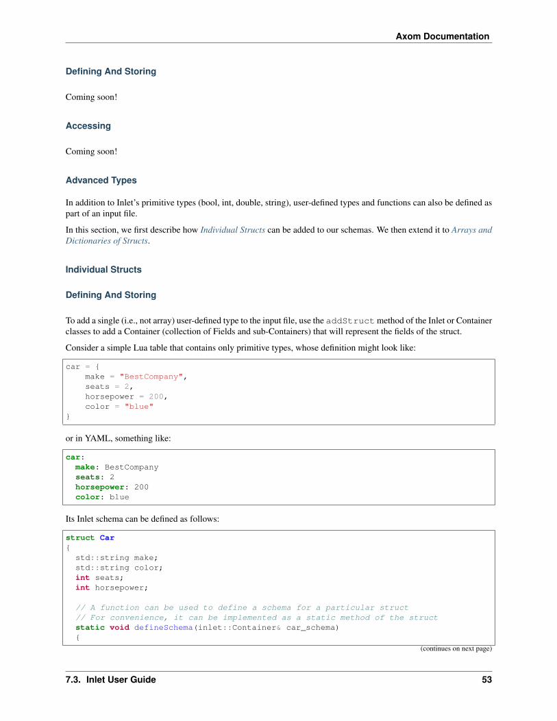
Axom Documentation


Coming soon!

Accessing

Coming soon!

Advanced Types

In addition to Inlet’s primitive types (bool, int, double, string), user-defined types and functions can also be defined aspart of an input file.

In this section, we first describe how Individual Structs can be added to our schemas. We then extend it to Arrays andDictionaries of Structs.

Individual Structs


To add a single (i.e., not array) user-defined type to the input file, use the addStructmethod of the Inlet or Containerclasses to add a Container (collection of Fields and sub-Containers) that will represent the fields of the struct.

Consider a simple Lua table that contains only primitive types, whose definition might look like:

car = make = "BestCompany",seats = 2,horsepower = 200,color = "blue"

or in YAML, something like:

car:make: BestCompanyseats: 2horsepower: 200color: blue

Its Inlet schema can be defined as follows:

struct Car

std::string make;std::string color;int seats;int horsepower;

// A function can be used to define a schema for a particular struct// For convenience, it can be implemented as a static method of the structstatic void defineSchema(inlet::Container& car_schema)



Axom Documentation


car_schema.addString("make", "Make of car");car_schema.addString("color", "Color of car").defaultValue("red");car_schema.addInt("seats", "Number of seats").range(2, 7);car_schema.addInt("horsepower", "Amount of horsepower");

;

This would be used by creating an inlet::Container for the Car instance and then defining the struct schemaon that subcontainer, e.g.:

// Create a container off the global container for the car object// then define its schemaauto& car_schema = inlet.addStruct("car", "Vehicle description");Car::defineSchema(car_schema);

Note: The definition of a static defineSchema member function is not required, and is just used for convenience.The schema definition for a class or struct could also be implemented as a free function for third-party types, or evenin the same place as the sub-container declaration.

Accessing

In order to convert from Inlet’s internal representation to a custom C++ struct, you must provide deserializationlogic. This is accomplished by a specialization of the FromInlet<T> functor for your type T, which implementsa member function with the signature T operator()(const inlet::Container&). This function shouldreturn an instance of type T with its members populated with the corresponding fields in the input file. For the simpleCar example whose schema is defined above, the specialization might look like:

template <>struct FromInlet<Car>

Car operator()(const inlet::Container& input_data)Car result;result.make = input_data["make"];result.color = input_data["color"];result.seats = input_data["seats"];result.horsepower = input_data["horsepower"];return result;

;

In the above snippet, Container::operator[] is used to extract data from Inlet’s internal representation whichis automatically converted to the correct member variable types when the function’s return value is constructed. Thisconversion does not happen automatically for user-defined types. If a Car object as defined above is located at thepath “car” within the input file, it can be retrieved as follows:

Car car = inlet["car"].get<Car>();

Arrays and Dictionaries of Structs

Arrays of user-defined types are also supported in Inlet.


Axom Documentation


Consider a collection of cars, described in Lua as:

fleet = make = "Globex Corp",seats = 3,horsepower = 155,color = "green"

,make = "Initech",seats = 4,horsepower = 370-- uses default value for color

,make = "Cyberdyne",seats = 1,horsepower = 101,color = "silver"

or in YAML, as:

fleet:- make: Globex Corpseats: 3horsepower: 155color: green

- make: Initechseats: 4horsepower: 370# uses default value for color

- make: Cyberdyneseats: 1horsepower: 101color: silver

First, use the addStructArray function to create a subcontainer, then define the schema on that container usingthe same Car::defineSchema used above:

// Create a fleet of cars with the same Car::defineSchemaauto& fleet_schema = inlet.addStructArray("fleet", "A collection of cars");Car::defineSchema(fleet_schema);

Note: The schema definition logic for a struct is identical between individual instances of structs and arrays of structs.The distinction is made by Container on which the struct schema is defined - specifically, whether it is obtainedvia addStruct or addStructArray.

Associative arrays are also supported, using string keys or a mixture of string and integer keys. TheaddStructDictionary function can be used analogously to the addStructArray function for these asso-ciative arrays.


Axom Documentation

Note: Although many of Inlet’s input file languages do not distinguish between a “dictionary” type and a “record”type, Inlet treats them differently for type safety reasons:

Dictionaries use arbitrary strings or integers for their keys, and their values (entries) can only be retreived as a homo-geneous type. In other words, dictionaries must map to std::unordered_map<Key, Value> for fixed key andvalue types.

Structs contain a fixed set of named fields, but these fields can be of any type. As the name suggests, these map tostructs in C++.

Accessing

As with the schema definition, the FromInlet specialization for a user-defined type will work for both single in-stances of the type and arrays of the type.

To retrieve an array of structs as a contiguous array of user-defined type, use std::vector:

auto fleet = base["fleet"].get<std::vector<Car>>();

Some input file languages support non-contiguous array indexing, so you can also retrieve arrays asstd::unordered_map<int, T>:

auto fleet = inlet["fleet"].get<std::unordered_map<int, Car>>();

Note: If a non-contiguous array is retrieved as a (contiguous) std::vector, the elements will be ordered byincreasing index.

String-keyed dictionaries are implemented as std::unordered_map<std::string, T> and can be retrievedin the same way as the array above. For dictionaries with a mix of string and integer keys, the inlet::VariantKeytype can be used, namely, by retrieving a std::unordered_map<inlet::VariantKey, T>.

Function Callbacks

For input file types that support functions, e.g., Lua, functions can also be read from the input file into astd::function, the wrapper for callables provided by the C++ standard library.


This is accomplished by calling addFunction on an Inlet or Container object.

Consider the following Lua function that accepts a vector in R2 or R3 and returns a double:

coef = function (v)if v.dim == 2 thenreturn v.x + (v.y * 0.5)

elsereturn v.x + (v.y * 0.5) + (v.z * 0.25)

endend

The schema for this function would be defined as follows:


Axom Documentation

schema.addFunction("coef",

inlet::FunctionTag::Double,inlet::FunctionTag::Vector, inlet::FunctionTag::Double,"The function representing the BC coefficient")

The return type and argument types are described with the inlet::FunctionTag enumeration, which has thefollowing members:

• Double - corresponds to a C++ double

• String - corresponds to a C++ std::string

• Vector - corresponds to a C++ inlet::InletVector

• Void - corresponds to C++ void, should only be used for functions that don’t return a value

Note that a single type tag is passed for the return type, while a vector of tags is passed for the argument types.Currently a maximum of two arguments are supported. To declare a function with no arguments, simply leave the listof argument types empty.

Note: The InletVector type (and its Lua representation) are statically-sized vectors with a maximum dimensionof three. That is, they can also be used to represent two-dimensional vectors.

In Lua, the following operations on the Vector type are supported (for Vector s u, v, and w):

1. Construction of a 3D vector: u = Vector.new(1, 2, 3)

2. Construction of a 2D vector: u = Vector.new(1, 2)

3. Construction of an empty vector (default dimension is 3): u = Vector.new()

4. Vector addition and subtraction: w = u + v, w = u - v

5. Vector negation: v = -u

6. Scalar multiplication: v = u * 0.5, v = 0.5 * u

7. Indexing (1-indexed for consistency with Lua): d = u[1], u[1] = 0.5

8. L2 norm and its square: d = u:norm(), d = u:squared_norm()

9. Normalization: v = u:unitVector()

10. Dot and cross products: d = u:dot(v), w = u:cross(v)

11. Dimension retrieval: d = u.dim

12. Component retrieval: d = u.x, d = u.y, d = u.z

Accessing

To retrieve a function, both the implicit conversion and get<T> syntax is supported. For example, a function can beretrieved as follows:

// Retrieve the function (makes a copy) to be moved into the lambdaauto func =base["coef"].get<std::function<double(FunctionType::Vector, double)>>();

It can also be assigned directly to a std::function without the need to use get<T>:


Axom Documentation

std::function<double(FunctionType::Vector)> coef = inlet["coef"];

Additionally, if a function does not need to be stored, the overhead of a copy can be eliminated by calling it directly:

double result = inlet["coef"].call<double>(axom::inlet::FunctionType::Vector3, 5, 7→˓);

Note: Using call<ReturnType>(ArgType1, ArgType2, ...) requires both that the return type be ex-plicitly specified and that argument types be passed with the exact type as used in the signature defined as part of theschema. This is because the arguments do not participate in overload resolution.

Verification

Before input file data can be accessed, it must first be verified by calling the verify() method of the top-levelInlet object. This will return a bool indicating whether the provided input conformed to the schema and specificviolations of the schema are logged via SLIC by default. If you would like to suppress the SLIC warnings and processthe list of verification errors instead, you can pass a std::vector<inlet::VerificationError> to theverify() method as follows:

std::vector<inlet::VerificationError> errors;inlet.verify(&errors);

You can then iterate over the list of errors, each of which contains the path within the input file of the offendingContainer, Field, or Function and the corresponding message.

This section describes the verification rules that apply to each possible element of the Inlet hierarchy, namely,Container, Field, and Function.

Container Verification

If a Container is marked as required (via the required()) method, then the Container must have a Fieldor Function that was present in the input or contain a sub-Container that does. This does not apply to aContainer that corresponds to an array or dictionary, as empty collections provided by the user are consideredvalid. Consider the following definition and input file:

addIntArray("foo").required();

foo =

Inlet verification will succeed for the above snippets.

If a Container corresponds to an array or dictionary, the elements of the array must all be of the requested type, ifany were provided. This restriction applies even if the array/dictionary was not marked as required.

If a verification function was provided via the registerVerifier() method, this function must return truewhen passed the corresponding Container object.

Note: Since a Container represents internal nodes in the Inlet hierarchy, its verification status is dependent on thatof its child objects. A Container is only considered valid if all of its child Container, Field, and Functionobjects are also valid.


Axom Documentation

Field Verification

If a Field is marked as required (via the required()) method, then a value must be provided in the input.

Providing a value of the wrong type will result in verification failure, even if the field was not marked as required.

If a range (inclusive upper/lower bounds) of valid values is specified with the range() method, both the providedvalue (if applicable) and default value (if specified with defaultValue()) must fall within the range.

If a set of valid values is specified with the validValues() method, both the provided value (if applicable) anddefault value (if specified with defaultValue()) must be included in the set.

If a verification function was provided via the registerVerifier() method, this function must return truewhen passed the corresponding Field object.

Function Verification

If a Function is marked as required (via the required()) method, then a function must be provided in the input.

If a verification function was provided via the registerVerifier() method, this function must return truewhen passed the corresponding Function object.

Unexpected Entries in Input Files

In order to better detect user error, e.g., misspelled names, Inlet provides a method to retrieve the names of entries inthe input file that were not requested in the schema definition phase. Consider the following input:

const std::string input = R"(dimensions = 2dim = 2 -- An example typo, should be "dimensions" and not "dim"vector = x = 1.0,y = 2.0,z = 3.0 -- Only 2 component vectors are supported

)";

The full set of unexpected names across the entire input file can be retrieved from the top-level Inlet object asfollows:

const std::vector<std::string> all_unexpected_names =myInlet.unexpectedNames(); // "dim", "vector/z"

The list of unexpected names can also be retrieved relative to an individual Container - that is, anywherewithin/below that container:

// defines a required container named vector with an internal field named 'x'auto& v = myInlet.addStruct("vector").required(true);

const std::vector<std::string> vector_unexpected_names =v.unexpectedNames(); // "vector/z"

These lists of unexpected names can be useful if you’d like to implement custom/targeted error messages - in theexample above, one might wish to provide a message indicating that dimension should be used instead of justdim. In other cases, it may be sufficient to just require that all or part of the input file have no unexpected entries.


Axom Documentation

This is supported via the strict() method, which will cause a Container to fail verification if it contains anyunexpected entries:

v.strict();

7.4 Klee User Guide

Klee provides a way to embed 2D and 3D non-conformal geometry in a mesh.

Contents:

7.4.1 Specifying Shapes

“Shaping”, or “painting”, is the process of adding non-conformal material regions to a mesh. Traditionally, this hasbeen done in code-specific formats by each code that provides such a capability. Axom’s Klee library provides a wayto read shape specifications in YAML files and apply the specified geometry to a mesh.

Basics

Shapes in Klee are specified in YAML. A basic file consists of a list of shapes. Each one specifies its name andmaterial, as well as a description of its geometry.

In addition to the shapes themselves, a file must specify the number of dimensions of the shapes (only 2 and 3 areallowed). This will be important later when specifying transformations and slices.

dimensions: 3

shapes:- name: wheelmaterial: steelgeometry:

format: stlpath: wheel.stlunits: cm

- name: windshieldmaterial: glassgeometry:

format: stlpath: windshield.stlunits: in

The above example describes a series of 3D shapes. The first is a wheel made of steel. Its geometry is specified in anSTL file named wheel.stl. Since STL files don’t have units embedded in them, we must specify them. The secondshape is named “windshield”, is made of “glass”, and its geometry is specified in windshield.stl. Note that Kleedoes not specify what a particular material means. A material is simply a label which can be used by a host code toapply properties to part of a mesh.

Paths

The paths specified in shapes are specified either as absolute paths (begin with a /), or as relative paths. Absolutepaths are evaluated as absolute paths in the file systems. Relative paths are evaluated relative to the YAML file (not


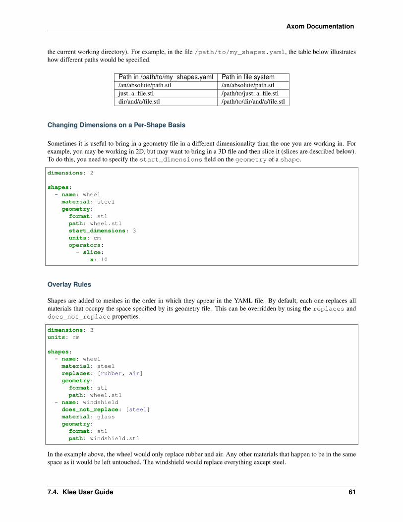
Axom Documentation

the current working directory). For example, in the file /path/to/my_shapes.yaml, the table below illustrateshow different paths would be specified.

Path in /path/to/my_shapes.yaml Path in file system/an/absolute/path.stl /an/absolute/path.stljust_a_file.stl /path/to/just_a_file.stldir/and/a/file.stl /path/to/dir/and/a/file.stl

Changing Dimensions on a Per-Shape Basis

Sometimes it is useful to bring in a geometry file in a different dimensionality than the one you are working in. Forexample, you may be working in 2D, but may want to bring in a 3D file and then slice it (slices are described below).To do this, you need to specify the start_dimensions field on the geometry of a shape.

dimensions: 2


format: stlpath: wheel.stlstart_dimensions: 3units: cmoperators:- slice:

x: 10

Overlay Rules

Shapes are added to meshes in the order in which they appear in the YAML file. By default, each one replaces allmaterials that occupy the space specified by its geometry file. This can be overridden by using the replaces anddoes_not_replace properties.

dimensions: 3units: cm

shapes:- name: wheelmaterial: steelreplaces: [rubber, air]geometry:

format: stlpath: wheel.stl

- name: windshielddoes_not_replace: [steel]material: glassgeometry:

format: stlpath: windshield.stl

In the example above, the wheel would only replace rubber and air. Any other materials that happen to be in the samespace as it would be left untouched. The windshield would replace everything except steel.

7.4. Klee User Guide 61

Axom Documentation

Warning: It is an error to specify both replaces and does_not_replace for the same shape.

Operators

When assembling complex geometries, it is often the case that different parts are specified in different coordinatesystems. For example, a description of the wheel of a car might be specified around its center, not its position relativeto the rest of the car. To help with this, Klee provides a mechanism to apply transformations to shapes.

dimensions: 3

shapes:- name: windshieldmaterial: glassgeometry:

format: stlpath: windshield.stlunits: cmoperators:- rotate: 90axis: [0, 1, 0]center: [0, 0, -10]

- translate: [10, 20, 30]

In the example above, the wheel is rotated 90 degrees counterclockwise around an axis centered at the point (0, 0,-10) and pointing in the direction of the vector (0, 1, 0). It is then translated by the vector (10, 20, 30).

Regardless of whether the geometry file has embedded units and what those may be, units must be specified wheneverspecifying operators. These are the units that will be used to interpret any lengths and points specified in operators.Units may be specified in one of two ways: by specifying units, or by specifying start_units and end_units.Specifying units is the same as giving the same value for start_units and end_units. Being able to changeunits is useful for situations where your geometry file is in one set units, but you’re thinking about your larger assemblyin another set of units. For example:

dimensions: 3

shapes:- name: windshieldmaterial: glassgeometry:

format: stlpath: windshield.stlstart_units: inend_units: ftoperators:# Orient the windshield about its own coordinate system,# working in its native units (inches)- translate: [10, 20, 30] # inches- rotate: 90axis: [0, 1, 0]center: [0, 0, -10] # inches

# switch to feet to put in the right place while thinking of# of the car in car in different units- convert_units_to: ft- translate: [2, 3, 4] # feet

It is an error if the end_units do not match the units after the last operator.


Axom Documentation

Supported Operators

The supported operators are listed below. Unless otherwise specified, the only difference between the 2D and 3Dversions are that whenever points or vectors are expected, the points and vectors must be of the dimensionality specifiedby the shape file.

Operators take the form of operator_name: value, where operator_name is the name of the operator,and value is the value specifying the parameters of the operation. Operators may also have additional required oroptional parameters.

• Translations

description Translate the shape by a given vector.

name translate

value a vector specifying the amount by which to translate the shape

example

# Translate by vector (1, 2, 3)translate: [1, 2, 3]

• Rotations

description Rotate the shape by a given amount around a specified axis

name rotate

value an angle, in degrees by which the shape will be rotated counterclockwise.

additional required parameters

axis (3D only) the axis of rotation

optional arguments

center a point specifying the center of rotation

example

# Rotate 45 degrees counterclockwise around the ray passing through# the point (1, 2, 3) and pointing in the direction of the vector# (4, 5, 6)rotate: 45center: [1, 2, 3]axis: [4, 5, 6]

• Scaling

description Scale the shape by a specified amount

name scale

value a vector specifying the amount by which to scale in each dimension, or a single value speci-fying by which to scale in all dimensions

example

# Scale by 2x in the x direction 0.5x in y, and 1.5x in zscale: [2.0, 0.5, 1.5]

• Changing Units


Axom Documentation

description Change the units in which subsequent operators are expressed. This is the same asscaling by the appropriate factor.

name convert_units_to

value the name of the units to convert to. Must be one of the named units.

example

geometry:...start_units: inend_units: cmoperators:- translate: [2, 3] # in inches- convert_units_to: cm # same as scale: 2.54- translate: [5, 6] # in centimeters

• Slices

description Slice a 3D object and convert it into a 2D object. This is accomplished by defining a cutplane which will be used to determine what slice of the geometry to take. In addition, a pointon the plane is picked as the new origin, and a vector is used to specify how the plane should beoriented with the 2D axes.

name slice

value an object with the the following properties

origin the point to use as the origin of the new coordinate system

normal a vector normal to the slice plane

up a vector which will be mapped to the positive Y direction on the cut plane.

optional arguments

x a single value specifying that the cut plane perpendicular to the x-axis at this value.See defaults table below.

y a single value specifying that the cut plane perpendicular to the y-axis at this value.See defaults table below.

z a single value specifying that the cut plane perpendicular to the z-axis at this value.See defaults table below.

If a plane is specified by just giving “x”, “y”, or “z”, then the origin, normal, and up vectorsare given the default values specified in the table below. They can be overridden so long as theorigin is still on the plane, and the normal is a multiple of the default normal.

Usage origin normal upx: <val> (<val>, 0, 0) (1, 0, 0) (0, 0, 1)y: <val> (0, <val>, 0) (0, 1, 0) (1, 0, 0)z: <val> (0, 0, <val>) (0, 0, 1) (0, 1, 0)

example

# Cut a 3D object with a plane that passes through the point# [10, 20, 30] and is normal to the vector [4, 5, 6]. The vector# [-5, 4, 0] will be mapped to the positive Y axis. [10, 20, 30] will# be mapped to the origin.



Axom Documentation


slice:origin: [10, 20, 30]normal: [4, 5, 6]up: [-5, 4, 0]

Named Operators

It can often be useful to name and reuse operators. For example, you may have several parts of an assembly specifiedin one coordinate system that you then need to transform to another. To enable reuse, we provide support for namedoperators.

Named operators are specified via the top-level named_operators object. This is a list where each entry has thefollowing values:

name (required) the name of the operator. This is how it is referenced later.

value (required) A list of operators. This is identical to the operators entry in the geometry objectof a shape.

start_dimensions (optional) the number of initial dimensions of the operator. Must be 2 or 3. If notspecified, the number of dimensions of the document is used.

units (required, must specify this or start_units and end_units) the units in which the operator isspecified

start_units (optional, must specify this or units) the units in which the first operator is specified

end_units (optional, must specify this or units) the units in which the last operator is specified. It is anerror if the units aren’t properly converted to end_units after applying all operations.

The example below demonstrates how to create and then use a named operator. Notice how we can use multiple refentries in the list of operators and we can intermix these with other operators as needed.

dimensions: 2

named_operators:- name: MyFirstOperatorunits: cmvalue:

- translate: [10, 20]- scale: 1.5

- name: AnotherOperatorunit: cmvalue:

- translate: [30, 40]


format: c2cpath: wheel.contourunits: cmoperators:- ref: MyFirstOperator- rotate: 90- ref: AnotherOperator


Axom Documentation

An important thing to note is that the units of the named operator and the shape that uses it do not have to match.The appropriate conversions will be done automatically if needed. This allows you to not worry about how thetransformation was defined when you use it.

dimensions: 2

named_operators:- name: MySampleOperatorstart_units: cmend_units: mmvalue:

- translate: [10, 20] # cm- convert_units_to: mm- translate: [30, 40] # mm


format: c2cpath: wheel.contourunits: inoperators:# Automatic conversion from in to cm- ref: MySampleOperator# Automatic conversion from mm to in- translate: [50, 60] # in

In addition to using ref in an individual shape’s operators, you can also use it in other named operators. The onlyrestriction is that it be defined in the list before it is used.

dimensions: 2units: cm

named_operators:- name: SomeOperatorunits: cmvalue:

- translate: [10, 20]- scale: 1.5

- name: AnotherOperatorunits: cmvalue:

- rotate: 90- ref: SomeOperator

7.5 Lumberjack User Guide

Lumberjack, named because it cuts down logs, is a C++ library that provides scalable logging while reducing theamount of messages written out the screen or file system.




../../../../doxygen/html/lumberjacktop.html

Axom Documentation

7.5.2 Introduction

Lumberjack was created to provide scalable logging with a simple programming model while allowing developers tocustomize its behavior. It is named Lumberjack because it cuts down logs. It uses MPI and a scalable binary treereduction scheme to combine duplicate messages and limit output to only the root node.

7.5.3 Requirements

• MPI - MPI is fundamental to Lumberjack and without MPI, Lumberjack is not useful.

7.5.4 Code Guarding

You tell if Axom was built with Lumberjack enabled by using the following include and compiler define:

#include "axom/config.hpp"#ifdef AXOM_USE_LUMBERJACK

// Lumberjack code#endif

Quick Start

This quick start guide goes over the bare minimum you need to do to get up and running with Lumberjack. You canfind this example in the repository under Lumberjack’s examples directory.

This example uses the Binary Tree Communicator and queues one unique message and three similar messages perrank. They are combined and then pushed fully through the tree.

The following files need to be included for Lumberjack:

# Lumberjack specific header#include "axom/lumberjack.hpp"

# MPI and C++#include <mpi.h>#include <iostream>

Basic MPI setup and information:

// Initialize MPI and get rank and comm sizeMPI_Init(&argc, &argv);

int commRank = -1;MPI_Comm_rank(MPI_COMM_WORLD, &commRank);int commSize = -1;MPI_Comm_size(MPI_COMM_WORLD, &commSize);

Initialize Lumberjack:

// Determine how many ranks we want to individually track per messageint ranksLimit = commSize/2;

// Initialize which lumberjack communicator we wantaxom::lumberjack::BinaryTreeCommunicator communicator;communicator.initialize(MPI_COMM_WORLD, ranksLimit);


7.5. Lumberjack User Guide 67

Axom Documentation


// Initialize lumberjackaxom::lumberjack::Lumberjack lj;lj.initialize(&communicator, ranksLimit);

This queues the individual messages into Lumberjack:

// Queue messages into lumberjackif (commRank == 0)

lj.queueMessage("This message will not be combined");else

lj.queueMessage("This message will be combined");lj.queueMessage("This message will be combined");lj.queueMessage("This message will be combined");

This is how you fully push all Messages through the Communicator, which also combines Messages before and afterpushing :

// Push messages fully through lumberjack's communicatorlj.pushMessagesFully();

Optionally, you could spread the pushing over the course of your work by doing the following:

int cycleCount = 0;int cycleLimit = 10;for (int i = 0; i < someLoopLength; ++i)

//// Do some work//lj.queueMessage("This message will combine")++cycleCount;if (cycleCount > cycleLimit)

// Incrementally push messages through systemlj.pushMessagesOnce();cycleCount = 0;

Once you are ready to retrieve your messages, do so by the following:

// Determine if this is an output nodeif (lj.isOutputNode())

// Get Messages from Lumberjackstd::vector<axom::lumberjack::Message*> messages = lj.getMessages();for(int i=0; i<(int)(messages.size()); ++i)

// Output a single Message at a time to screenstd::cout << "(" << messages[i]->stringOfRanks() << ") " << messages[i]->

→˓count() <<" '" << messages[i]->text() << "'" << std::endl;

// Clear already outputted Messages from Lumberjacklj.clearMessages();

Finalize Lumberjack, the Lumberjack Communicator and MPI in the following order to guarantee nothing goes wrong:


Axom Documentation

// Finalize lumberjacklj.finalize();// Finalize the lumberjack communicatorcommunicator.finalize();// Finalize MPIMPI_Finalize();

Core Concepts

The following are core concepts required to understand how Lumberjack works.

Combining

Combining Messages is how Lumberjack cuts down on the number of Messages output from your program. It doesso by giving the currently held Messages at the current node, two at a time, to the Combiner classes that are currentlyregistered to Lumberjack when a Push happens.

Lumberjack only provides one Combiner, the TextEqualityCombiner. You can write your own Combiners and registerthem with Lumberjack. The idea is that each Combiner would have its own criteria for whether a Message should becombined and how to combine that specific Message with another of the same type.

Combiner’s have two main functions, shouldMessagesBeCombined and combine.

The function shouldMessagesBeCombined, returns True if the pair of messages satisfy the associated criteria. Forexample in the TextEqualityCombiner, if the Text strings are exactly equal, it signals they should be combined.

The function combine, takes two Messages and combines them in the way that is specific to that Combiner class. Forexample in the TextEqualityCombiner, the only thing that happens is the second Message’s ranks gets added to thefirst and the message count is increased. This is because the text strings were equal. This may not be the case for allCombiners that you write yourself.

Communication

Communicating Messages between nodes in an intelligent way is how Lumberjack scales logging Messages. TheCommunicator class instance handles the specifics on how the communication is implemented. For example, it handleswhere a specific node passes its Messages and which nodes are allowed to output messages. As of now, there are twoimplemented Communicators: BinaryTreeCommunicator and RootCommunicator.

BinaryTreeCommunicator, as the name implies, utilizes a standard Binary Tree algorithm to define how the nodes areconnected. Children pass their Messages to their parent and the root node is the only node allowed to output Messages.

RootCommunicator has a very simple communication scheme that does not scale well but is useful in some cases forits simplicity. All nodes connect directly to the root node which is also the only node allowed to output Messages.

Pushing

A push has three steps: combining, sending, and receiving Messages. When you queue a Message into Lumberjack, itis held at the node that generated the Message until you indicate the Lumberjack to push, either once or fully. If youdo not push, then only the Messages generated at the root node will be outputed.

In a single push, nodes send their currently held Messages to the nodes their are connected to based on the Communi-cator’s communcation scheme. For example in the BinaryTreeCommunicator, children nodes send their Messages to


Axom Documentation

their parent. While the root node only receives Messages. After a single push, it is not guaranteed that all Messageswill be ready to be outputted.

A full push is a number of single pushes until all currently held Messages. The Communicator tells the Lumberjackclass how many single pushes it takes to fully flush the system of Messages. For example in the BinaryTreeCommu-nicator, it is the log of the number of nodes.

Lumberjack Classes

Basic

• Lumberjack - Performs all high level functionality for the Lumberjack library.

• Message - Holds all information pertaining to a Message.

Combiners

Handles Message combination and tests whether Message classes should be combined.

• Combiner - Abstract base class that all Combiners must inherit from.

• TextEqualityCombiner - Combines Message classes that have equal Text member variables.

Communicators

Handles all node-to-node Message passing.

• Communicator - Abstract base class that all Communicators must inherit from.

• BinaryTreeCommunicator - Main Communicator that is implemented with a scalable Binary Tree scheme.

• RootCommunicator - non-scalable communication scheme that all nodes connect to the root node. This is givenfor diagnostic purposes only.

Lumberjack Class

The Lumberjack class is where all high-level functionality of the library is done, such as adding, retrieving, andcombining messages and telling the given Communicator to push Messages through the communication scheme. Youcan also add and remove Combiner classes, as well as tell if the current node is supposed to output any messages.

Functions

General

Name Descriptioninitialize Starts up Lumberjack. Must be called before anything else.finalize Cleans up Lumberjack. Must be called when done with Lumberjack.isOutputNode Returns whether this node should output messages.ranksLimit Sets the limit on individually tracked ranksranksLimit Gets the limit on individually tracked ranks


Axom Documentation

Combiners

Name DescriptionaddCombiner Adds a combiner to LumberjackremoveCombiner Removes a specific combiner from LumberjackclearCombiners Removes all currently registered Combiners from Lumberjack

Messages

Name DescriptionclearMessages Delete all Messages currently held by this node.getMessages Get all Messages currently held by this node.queueMessage Adds a Message to LumberjackpushMessagesOnce Moves Messages up the communication scheme oncepushMessagesFully Moves all Messages through the communication scheme to the output node.

Combiner Class

The Combiner class is an abstract base class that defines the interface for all Combiner classes. Concrete instancesneed to inherit from this class and implement these functions to be used when Message classes are combined by theLumberjack class.

Functions

Name Descriptionid Returns the unique differentiating identifier for the class instance.shouldMessagesBeCombined Indicates if two messages should be combined.combine Combines the second message into the first.

Concrete Instances

TextEqualityCombiner

This Combiner combines the two given Messages if the Message text strings are equal. It does so by adding the secondMessage’s ranks to the first Message (if not past the ranksLimit) and incrementing the Message’s count as well. Thisis handled by Message.addRanks().

Note: This is the only Combiner automatically added to Lumberjack for you. You can remove it by calling Lumber-jack::removeCombiner(“TextEqualityCombiner”).

Communicator Class

The Communicator class is an abstract base class that defines the interface for all Communicator classes. Concreteinstances need to inherit from this class and implement these functions to be used when the Lumberjack class does


Axom Documentation

any communication work.

Functions

Name Descriptioninitialize Starts up the Communicator. Must be called before anything else.finalize Cleans up the Communicator. Must be called when finished.rank Returns the rank of the current node.ranksLimit Getter/Setter for the limit on individually stored ranks.numPushesToFlush Returns the number of individual pushes to completely flush all Messages.push Pushes all currently held Messages once up structure.isOutputNode Returns whether this node should output messages.

Concrete Instances

BinaryTreeCommunicator

Note: This is the recommended Communicator.

This Communicator uses a standard Binary Tree design to scalably pass Messages between nodes. Rank 0 is theroot of the Binary Tree and the only node allowed to output messages. For each single push, the child nodes sendtheir currently held messages to their parents without waiting to receive messages themselves. For a full push, thiscommunicator takes the log of nodes to completely flush all currently held messages to the root node.

RootCommunicator

Note: This Communicator is useful for debugging purposes, but will not scale as well as the recommended Binary-TreeCommunicator.

This Communicator has all nodes directly connecting to the root node which is rank 0. The root node is the only nodeallowed to output messages. Each single push, the child nodes send their currently held messages to the root. Aftereach push the tree is completely flushed.

Message Class

The Message class holds the information about a single message or multiple messages that were combined via aCombiner instance.

Information

The Message class contains the following information. All fields have their respective getters and setters.


Axom Documentation

Name Descriptiontext Contents of the messageranks Truncated list of where the message originatedcount Total count of how many individual messages occurredfileName File name that generated the messagelineNumber Line number that generated the messagelevel Message severity (error, warning, debug, etc.)tag Tag for showing what part of the code generated the message

Functions

The Message class also contains the following helper functions to ease use of the class.

Name DescriptionstringOfRanks Returns a string of the rankspack Returns a packed version of all the message’s informationunpack Takes a packed message and overwrites all the message’s informationaddRank Add a rank to the message to the given limitaddRanks Add ranks to the message to the given limit

7.6 Mint User Guide

Mint provides a comprehensive mesh data model and a mesh-aware, fine-grain, parallel execution model that underpinsthe development of computational tools and numerical discretization methods. Thereby, enable implementations thatare born parallel and portable to new and emerging architectures.



7.6.2 Key Features

• Support for 1D/2D/3D mesh geometry.

• Efficient data structures to represent Particle Mesh, Structured Mesh and Unstructured Mesh types, includingunstructured meshes with Mixed Cell Type Topology.

• Native support for a variety of commonly employed Cell Types.

• A flexible Mesh Storage Management system, which can optionally inter-operate with Sidre as the underlying,in-memory, hierarchical datastore, facilitating the integration across packages.

• Basic support for Finite Elements, consisting of commonly employed shape functions and quadratures.

• A Mesh-Aware Execution Model, based on the RAJA programming model abstraction layer that supports on-node parallelism for mesh-traversals, enabling the implementation of computational kernels that are born paralleland portable across different processor architectures.

7.6. Mint User Guide 73

../../../../doxygen/html/minttop.html

../../../sidre/docs/sphinx/index.html


Axom Documentation

7.6.3 Requirements

Mint is designed to be light-weight and self-contained. The only requirement for using Mint is a C++11 compli-ant compiler. However, to realize the full spectrum of capabilities, support for the following third-party libraries isprovided:

• RAJA, used for the parallel execution and portability layer.

• Conduit , for using Sidre as the Mesh Storage Management system.

• Umpire, for memory management on next-generation architectures.

For further information on how to build the Axom Toolkit using these third-party libraries, consult the Axom QuickStart Guide.

7.6.4 About this Guide

This guide discusses the basic concepts and architecture of Mint.

• The Getting Started with Mint section provides a quick introduction to Mint, designed to illustrate high-levelconcepts and key capabilities, in the context of a small working example.

• The Tutorial section provides code snippets that demonstrate specific topics in a structured and simple format.

• For complete documentation of the interfaces of the various classes and functions in Mint consult the MintDoxygen API Documentation.

• Complete examples and code walk-throughs of mini-apps using Mint are provided in the Examples section.

Additional questions, feature requests or bug reports on Mint can be submitted by creating a new issue on Github orby sending e-mail to the Axom Developers mailing list at [email protected].

Getting Started with Mint

This section presents a complete code walk-through of an example Mint application, designed to illustrate someof the key concepts and capabilities of Mint. The complete Mint Application Code Example, is included in the Ap-pendix section and is also available in the Axom source code under src/axom/mint/examples/user_guide/mint_getting_started.cpp.

The example Mint application demonstrates how Mint is used to develop kernels that are both mesh-agnostic anddevice-agnostic.

Tip: Mint’s RAJA-based Execution Model helps facilitate the implementation of various computational kernels thatare both mesh-agnostic and device-agnostic. Both kernels discussed in this example do not make any assumptionsabout the underlying mesh type or the target execution device, e.g. CPU or GPU. Consequently, the same implemen-tation can operate on both Structured Mesh and Unstructured Mesh types and run sequentially or in parallel on allexecution devices supported through RAJA.

Prerequisites

Understanding the discussion and material presented in this section requires:

• Working knowledge of C++ templates and Lambda Expression functions.

• High-level understanding of nested memory hierarchies on heterogeneous architectures and CUDA UnifiedMemory.



https://llnl-conduit.readthedocs.io/en/latest/index.html

../../../sidre/docs/sphinx/index.html

https://umpire.readthedocs.io/en/develop/

../../../../index.html

../../../../docs/sphinx/quickstart_guide/index.html





mailto:[email protected]



https://www.cprogramming.com/c++11/c++11-lambda-closures.html

https://devblogs.nvidia.com/unified-memory-cuda-beginners/


Axom Documentation

• Basics of the Execution Model (recommended)

Note: Mint does not provide a memory manager. The application must explicitly specify the desired allocationstrategy and memory space to use. This is facilitated by using Umpire for memory management. Specifically, thisexample uses CUDA Unified Memory when compiled with RAJA and CUDA enabled by setting the default Umpireallocator in the beginning of the program as follows:

// NOTE: use unified memory if we are using CUDAconst int allocID = axom::execution_space<ExecPolicy>::allocatorID();axom::setDefaultAllocator(allocID);

When Umpire , RAJA and CUDA are not enabled, the code will use the malloc() internally to allocate memory onthe host and all kernels will be executed on the CPU.

Goals

Completion of the walk-though of this simple code example should only require a few minutes. Upon completion, theuser will be familiar with using Mint to:

• Create and evaluate fields on a mesh

• Use the Node Traversal Functions and Cell Traversal Functions of the Execution Model to implement kernelsthat operate on the mesh and associated fields.

• Plot the mesh and associated fields in VTK for visualization.

Step 1: Add Header Includes

First, the Mint header must be included for the definition of the various Mint classes and functions. Note, this examplealso makes use of Axom’s Matrix class, which is also included by the following:

1 #include "axom/config.hpp" // compile time definitions2 #include "axom/core/execution/execution_space.hpp" // for execution_space traits3

4 #include "axom/mint.hpp" // for mint classes and functions5 #include "axom/core/numerics/Matrix.hpp" // for numerics::Matrix

Step 2: Get a Mesh

The example application is designed to operate on either a Structured Mesh or an Unstructured Mesh. The type ofmesh to use is specified by a runtime option that can be set by the user at the command line. See Step 7: Run theExample for more details.

To make the code work with both Structured Mesh and Unstructured Mesh instances the kernels are developed in termsof the The Mesh Base Class, mint::Mesh.

The pointer to a mint::Mesh object is acquired as follows:

1 mint::Mesh* mesh =2 (Arguments.useUnstructured) ? getUnstructuredMesh() : getUniformMesh();

When using a Uniform Mesh, the mesh is constructed by the following:








Axom Documentation

1 mint::Mesh* getUniformMesh()2 3 // construct a N x N grid within a domain defined in [-5.0, 5.0]4 const double lo[] = -5.0, -5.0;5 const double hi[] = 5.0, 5.0;6 mint::Mesh* m = new mint::UniformMesh(lo, hi, Arguments.res, Arguments.res);7 return (m);8

This creates an 𝑁 ×𝑁 Uniform Mesh, defined on a domain given by the interval ℐ : [−5.0, 5.0] × [−5.0, 5.0], where𝑁 = 25, unless specified otherwise by the user at the command line.

When an Unstructured Mesh is used, the code will generate the Uniform Mesh internally and triangulate it by subdi-viding each quadrilateral element into four triangles. See the complete Mint Application Code Example for details.

See the Tutorial for more details on how to Create a Uniform Mesh or Create an Unstructured Mesh.

Step 3: Add Fields

Fields are added to the mesh by calling the createField() method on the mesh object:

1 // add a cell-centered and a node-centered field2 double* phi = mesh->createField<double>("phi", mint::NODE_CENTERED);3 double* hc = mesh->createField<double>("hc", mint::CELL_CENTERED);4

5 constexpr int NUM_COMPONENTS = 2;6 double* xc =7 mesh->createField<double>("xc", mint::CELL_CENTERED, NUM_COMPONENTS);

• The node-centered field, phi, stores the result, computed in Step 4: Evaluate a Scalar Field

• The cell-centered field, hc, stores the nodal average of phi, computed in Step 5: Average to Cell Centers

• The cell-centered field, xc, stores the cell-centers, computed in Step 5: Average to Cell Centers

Note, the template argument to the createField() method indicates the underlying field type, e.g. double, int, etc. In this case, all three fields have a double field type.

The first required argument to the createField() method is a string corresponding to the name of the field. Thesecond argument, which is also required, indicates the centering of the field, i.e. node-centered, cell-centered orface-centered.

A third, optional, argument may be specified to indicate the number of components of the corresponding field. Inthis case, the node-centered field, phi, is a scalar field. However, the cell-centered field, xc, is a 2D vector quantity,which is specified explicitly by supplying the third argument in the createField() method invocation.

Note: Absence of the third argument when calling createField() indicates that the number of components ofthe field defaults to 1 and thereby the field is assumed to be a scalar quantity.

See the Tutorial for more details on Working with Fields on a mesh.

Step 4: Evaluate a Scalar Field

The first kernel employs the for_all_nodes() traversal function of the Execution Model to iterate over the con-stituent mesh Nodes and evaluate Himmelblau’s Function at each node:


https://en.wikipedia.org/wiki/Himmelblau%27s_function

Axom Documentation

1 // loop over the nodes and evaluate Himmelblaus Function2 mint::for_all_nodes<ExecPolicy, xargs::xy>(3 mesh,4 AXOM_LAMBDA(IndexType nodeIdx, double x, double y) 5 const double x_2 = x * x;6 const double y_2 = y * y;7 const double A = x_2 + y - 11.0;8 const double B = x + y_2 - 7.0;9

10 phi[nodeIdx] = A * A + B * B;11 );

• The arguments to the for_all_nodes() function consists of:

1. A pointer to the mesh object, and

2. The kernel that defines the per-node operations, encapsulated within a Lambda Expression, using theconvenience AXOM_LAMBDA Macro.

• In addition, the for_all_nodes() function has two template arguments:

1. ExecPolicy: The execution policy specifies, where and how the kernel is executed. It is a requiredtemplate argument that corresponds to an Execution Policy defined by the Execution Model.

2. xargs::xy: Indicates that in addition to the index of the node, nodeIdx, the kernel takes the x and ynode coordinates as additional arguments.

Within the body of the kernel, Himmelblau’s Function is evaluated using the supplied x and y node coordinates. Theresult is stored in the corresponding field array, phi, which is captured by the Lambda Expression, at the correspond-ing node location, phi[ nodeIdx ].

See the Tutorial for more details on using the Node Traversal Functions of the Execution Model.

Step 5: Average to Cell Centers

The second kernel employs the for_all_cells() traversal function of the Execution Model to iterate over theconstituent mesh Cells and performs the following:

1. computes the corresponding cell centroid, a 2D vector quantity,

2. averages the node-centered field, phi, computed in Step 4: Evaluate a Scalar Field, at the cell center.

1 // loop over cells and compute cell centers2 mint::for_all_cells<ExecPolicy, xargs::coords>(3 mesh,4 AXOM_LAMBDA(IndexType cellIdx,5 const numerics::Matrix<double>& coords,6 const IndexType* nodeIds) 7 // NOTE: A column vector of the coords matrix corresponds to a nodes coords8

9 // Sum the cell's nodal coordinates10 double xsum = 0.0;11 double ysum = 0.0;12 double hsum = 0.0;13

14 const IndexType numNodes = coords.getNumColumns();15 for(IndexType inode = 0; inode < numNodes; ++inode)16 17 const double* node = coords.getColumn(inode);






Axom Documentation


18 xsum += node[mint::X_COORDINATE];19 ysum += node[mint::Y_COORDINATE];20

21 hsum += phi[nodeIds[inode]];22 // END for all cell nodes23

24 // compute cell centroid by averaging the nodal coordinate sums25 const IndexType offset = cellIdx * NUM_COMPONENTS;26 const double invnnodes = 1.f / static_cast<double>(numNodes);27 xc[offset] = xsum * invnnodes;28 xc[offset + 1] = ysum * invnnodes;29

30 hc[cellIdx] = hsum * invnnodes;31 );

• Similarly, the arguments to the for_all_cells() function consists of:

1. A pointer to the mesh object, and

2. The kernel that defines the per-cell operations, encapsulated within a Lambda Expression, using the con-venience AXOM_LAMBDA Macro.

• In addition, the for_all_cells() function has two template arguments:

1. ExecPolicy: As with the for_all_nodes() function, the execution policy specifies, where andhow the kernel is executed.

2. xargs::coords: Indicates that in addition to the index of the cell, cellIdx, the supplied kernel takestwo additional arguments:

a. coords, a matrix that stores the node coordinates of the cell, and

b. nodeIds, an array that stores the IDs of the constituent cell nodes.

The cell node coordinates matrix, defined by axom::numerics::Matrix is organized such that:

• The number of rows of the matrix corresponds to the cell dimension, and,

• The number of columns of the matrix corresponds to the number of cell nodes.

• The 𝑖𝑡ℎ column vector of the matrix stores the coordinates of the 𝑖𝑡ℎ cell node.

In this example, the 2D Uniform Mesh, consists of 2D rectangular cells, which are defined by 4 nodes. Consequently,the supplied node coordinates matrix to the kernel, coords, will be a 2 × 4 matrix of the following form:(

𝑥0 𝑥1 𝑥2 𝑥3

𝑦0 𝑦1 𝑦2 𝑦3

)Within the body of the kernel, the centroid of the cell is calculated by averaging the node coordinates. The code loopsover the columns of the coords matrix (i.e., the cell nodes) and computes the sum of each node coordinate in xsumand ysum respectively. Then, the average is evaluated by multiplying each coordinate sum with 1/𝑁 , where 𝑁 is thenumber of nodes of a cell. The result is stored in the corresponding field array, xc, which is captured by the LambdaExpression.

Since, the cell centroid is a 2D vector quantity, each cell entry has an x-component and y-component. Multi-componentfields in Mint are stored using a 2D row-major contiguous memory layout, where, the number of rows corresponds tothe number of cells, and the number of columns correspond to the number of components of the field. Consequently,the x-component of the centroid of a cell with ID, cellIdx is stored at xc[ cellIIdx * NUM_COMPONENTS ]and the y-component is stored at xc[ cellIdx * NUM_COMPONENTS + 1 ], where NUM_COMPONENTS=2.





Axom Documentation

In addition, the node-centered quantity, phi, computed in Step 4: Evaluate a Scalar Field is averaged and stored atthe cell centers. The kernel first sums all the nodal contributions in hsum and then multiplies by 1/𝑁 , where 𝑁 is thenumber of nodes of a cell.

See the Tutorial for more details on using the Cell Traversal Functions of the Execution Model.

Step 6: Output the Mesh in VTK

Last, the resulting mesh and data can be output in the Legacy VTK File Format, which can be visualized by a varietyof visualization tools, such as VisIt and ParaView as follows:

1 // write the mesh in a VTK file for visualization2 std::string vtkfile =3 (Arguments.useUnstructured) ? "unstructured_mesh.vtk" : "uniform_mesh.vtk";4 mint::write_vtk(mesh, vtkfile);

A VTK file corresponding to the VTK File Format specification for the mesh type used will be generated.

Step 7: Run the Example

After building the Axom Toolkit, the basic Mint example may be run from within the build space directory as follows:

> ./examples/mint_getting_started_ex

By default the example will use a 25 × 25 Uniform Mesh domain defined on the interval ℐ : [−5.0, 5.0] × [−5.0, 5.0].The resulting VTK file is stored in the specified file, uniform_mesh.vtk. A depiction of the mesh showing a plotof Himmelblau’s Function computed over the constituent Nodes of the mesh is illustrated in Fig. 7.1.

The user may choose to use an Unstructured Mesh instead by specifying the --unstructured option at the com-mand line as follows:

> ./examples/mint_getting_started_ex --unstructured

The code will generate an Unstructured Mesh by triangulating the Uniform Mesh such that each quadrilateral is sub-divided into four triangles. The resulting unstructured mesh is stored in a VTK file, unstructured_mesh.vtk,depicted in Fig. 7.2.

By default the resolution of the mesh is set to 25 × 25. A user may set the desired resolution to use at the commandline, using the --resolution [N] command line option.

For example, the following indicates that a mesh of resolution 100 × 100 will be used instead when running theexample.

> ./examples/mint_getting_started_ex --resolution 100

Note: This example is designed to run:

• In parallel on the GPU when the Axom Toolkit is compiled with RAJA and CUDA enabled.

• In parallel on the CPU when the Axom Toolkit is compiled with RAJA and OpenMP enabled.

• Sequentially on the CPU, otherwise.


https://vtk.org/Wiki/images/5/51/VTK-File-Formats.pdf

https://wci.llnl.gov/simulation/computer-codes/visit

https://www.paraview.org/


../../../../../index.html


../../../../../index.html


../../../../../index.html


Axom Documentation

Fig. 7.1: Plot of Himmelblau’s Function computed over the constituent Nodes of the Uniform Mesh.



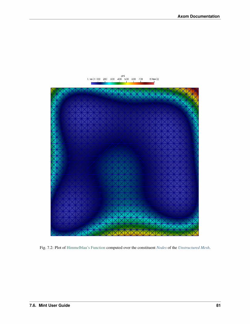
Axom Documentation

Fig. 7.2: Plot of Himmelblau’s Function computed over the constituent Nodes of the Unstructured Mesh.



Axom Documentation

Preliminary Concepts

A mesh (sometimes also called a grid), denoted by ℳ(Ω), provides a discrete represenation of a geometric domain ofinterest, Ω, on which, the underlying mathematical model is evaluated. The mathematical model is typically definedby a system of governing Partial Differential Equations (PDEs) and associated boundary and initial conditions. Thesolution to the governing PDE predicts a physical process that occurs and evolves on Ω over time. For example,consider the flow around an aircraft, turbulence modeling, blast wave propagation over complex terrains, or, heattransfer in contacting objects, to name a few. Evolving the mathematical model to predict such a physical process istypically done numerically, which requires discretizing the governing PDE by a numerical scheme, such as a FiniteDifference (FD), Finite Volume (FV), or, the Finite Element Method (FEM), chief among them.

Fig. 7.3: Mesh discretization of a geometric domain: (a) Sample geometric domain, Ω. (b) Corresponding mesh ofthe domain, ℳ(Ω). The nodes and cells of the mesh, depicted in red, correspond to the discrete locations where theunknown variables of the governing PDE are stored and evaluated.

Discretization of the governing PDE requires the domain to be approximated with a mesh. For example, Fig. 7.3 (a)depicts a geometric domain, Ω. The corresponding mesh, ℳ(Ω), is illustrated in Fig. 7.3 (b). The mesh approximatesthe geometric domain, Ω, by a finite number of simple geometric entities, such as nodes and cells, depicted in red inFig. 7.3 (b). These geometric entities comprising the mesh define the discrete locations, in space and time, at whichthe unknown variables, i.e., the degrees of freedom of the governing PDE, are evaluated, by the numerical schemebeing employed.

There are a variety of different Mesh Types one can choose from. The type of mesh employed depends on the choice ofthe underlying numerical discretization scheme. For example, a finite difference scheme typically requires a StructuredMesh. However, the finite volume and finite element methods may be implemented for both Structured Mesh andUnstructured Mesh types. In contrast, meshless or mesh-free methods, such as Smoothed Particle Hydrodynamics(SPH), discretize the governing PDE over a set of particles or nodes, using a Particle Mesh representation.


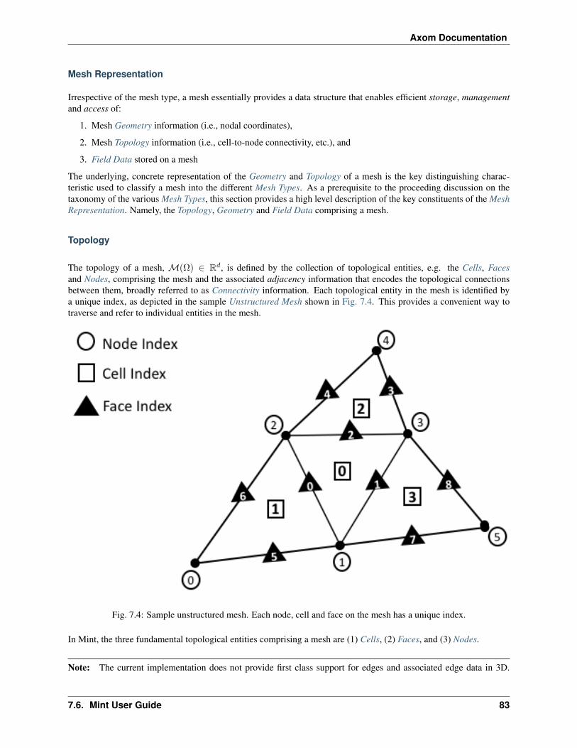
Axom Documentation

Mesh Representation

Irrespective of the mesh type, a mesh essentially provides a data structure that enables efficient storage, managementand access of:

1. Mesh Geometry information (i.e., nodal coordinates),

2. Mesh Topology information (i.e., cell-to-node connectivity, etc.), and

3. Field Data stored on a mesh

The underlying, concrete representation of the Geometry and Topology of a mesh is the key distinguishing charac-teristic used to classify a mesh into the different Mesh Types. As a prerequisite to the proceeding discussion on thetaxonomy of the various Mesh Types, this section provides a high level description of the key constituents of the MeshRepresentation. Namely, the Topology, Geometry and Field Data comprising a mesh.

Topology

The topology of a mesh, ℳ(Ω) ∈ R𝑑, is defined by the collection of topological entities, e.g. the Cells, Facesand Nodes, comprising the mesh and the associated adjacency information that encodes the topological connectionsbetween them, broadly referred to as Connectivity information. Each topological entity in the mesh is identified bya unique index, as depicted in the sample Unstructured Mesh shown in Fig. 7.4. This provides a convenient way totraverse and refer to individual entities in the mesh.

Fig. 7.4: Sample unstructured mesh. Each node, cell and face on the mesh has a unique index.

In Mint, the three fundamental topological entities comprising a mesh are (1) Cells, (2) Faces, and (3) Nodes.

Note: The current implementation does not provide first class support for edges and associated edge data in 3D.


Axom Documentation

However, this is a feature we are planning to support in future versions of Mint.

Cells

A cell, 𝒞𝑖, is given by an ordered list of Nodes, 𝒞𝑖 = 𝑛0, 𝑛1, ...𝑛𝑘, where each entry, 𝑛𝑗 ∈ 𝒞𝑖, corresponds toa unique node index in the mesh. The order of Nodes defining a cell is determined according to a prescribed localnumbering convention for a particular cell type. See Fig. 7.15 and Fig. 7.16. All Mint Cell Types follow the CGNSNumbering Conventions.

Faces

Similarly, a face, ℱ𝑖, is defined by an ordered list of Nodes, ℱ𝑖 = 𝑛0, 𝑛1, ..., 𝑛𝑘. Faces are essentially Cells whosetopological dimension is one less than the dimension of the Cells they are bound to. See Fig. 7.5. Consequently, theconstituent faces of a 3D cell are 2D topological entities, such as triangles or quads, depending on the cell type. Thefaces of a 2D cell are 1D topological entities, i.e. segments. Last, the faces of a 1D cell are 0D topological entities, i.e.Nodes.

Note: In 1D the Faces of a cell are equivalent to the constituent mesh Nodes, hence, Mint does not explicitly supportFaces in 1D.

Fig. 7.5: Constituent faces of a cell in 2D and 3D respectively. the constituent faces of a 3D cell are 2D topologicalentities, such as triangles or quads, depending on the cell type. The faces of a 2D cell are 1D topological entities, i.e.segments.

Face Types

A mesh face can be bound to either one or two Cells:


https://cgns.github.io/CGNS_docs_current/sids/conv.html#unstructgrid.


Axom Documentation

• Faces bound to two Cells, within the same domain, are called internal faces.

• Faces bound to two Cells, across different domains (or partitions), are called internal boundary faces. Internalboundary faces define the communication boundaries where ghost data is exchanged between domains.

• Faces bound to a single cell are called external boundary faces. External boundary faces (and/or their con-sistuent nodes) are typically associated with a boundary condition.

Face Orientation

As with Cells, the ordering of the constituent nodes of a face is determined by the cell type. However, by convention,the orientation of a face is according to an outward pointing face normal, as illustrated in Fig. 7.6.

Fig. 7.6: Face Orientation. (a) From the viewpoint of a cell, its constituent faces are oriented according to anoutward facing normal. (b) From the viewpoint of a face, a face is oriented according to an outward facing normalwith respect to the first cell abutting to the face, denoted by, 𝒞0.

From the viewpoint of a cell, 𝒞𝑘, its constituent faces, defined in the local node numbering of the cell, are orientedaccording to an outward facing normal with respect to the cell, 𝒞𝑘. For example, in Fig. 7.6 (a), the triangle, 𝒞𝑘,has three faces that are oriented according to an outward facing normal and defined using local node numbers withrespect to their cell as follows, ℱ0 = 0, 1, ℱ1 = 1, 2 and ℱ2 = 2, 0

As noted earlier, a face can have at most two adjacent Cells, denoted by 𝒞0 and 𝒞1. By convention, from theviewpoint of a face, ℱ𝑘, defined using global node numbers, the face is oriented according to an outward facingnormal with respect to the cell corresponding to 𝒞0. As depicted in Fig. 7.6 (b), the face denoted by ℱ𝑘 has anoutward facing normal with respect to 𝒞0, consequently it is defined as follows, ℱ𝑘 = 1, 2.

Note: By convention, 𝒞1 is set to −1 for external boundary faces, which are bound to a single cell.


Axom Documentation

Nodes

The Nodes are zero dimensional topological entities and hence, are the lowest dimensional constituententities of a mesh. The Nodes are associated with the spatial coordinates of the mesh and are used indefining the topology of the higher dimensional topological entities comprising the mesh, such as theCells, Faces, etc., as discussed earlier. In a sense, the Nodes provide the means to link the Topology of themesh to its constituent Geometry and thereby instantiate the mesh in physical space.

Definition

A mesh node, ∖⟩, is associated with a point, 𝑝𝑖 ∈ R𝑑 and provides the means to:

1. Link the Topology of the mesh to its constituent Geometry

2. Support one or more degrees of freedom, evaluated at the given node location.

Notably, the nodes of a mesh may be more than just the vertices of the mesh. As discussed in the Preliminary Conceptssection, a mesh is a discretization of a PDE. Recall, the primary purpose of the mesh is to define the discrete locations,in both space and time, at which the unknown variables or degrees of freedom of the governing PDE are evaluated.Depending on the numerical scheme employed and the Cell Types used, additional mesh Nodes may be located on theconstituent cell faces, edges and in the cell interior. For example, in the Finite Element Method (FEM), the nodes forthe linear Lagrange Finite Elements, see Fig. 7.15, are located at the cell vertices. However, for quadratic Cell Types,see Fig. 7.16, the Lagrange 𝑃 2 finite element, for the quadrilateral and hexahedron (in 3D) cells, includes as Nodes,the cell, face and edge (in 3D) centroids in addition to the cell vertices. Other higher order finite elements may involveadditional nodes for each edge and face as well as in the interior of the cell.

Connectivity

The topological connections or adjecencies between the Cells, Faces and Nodes comprising the mesh, give rise to ahierarchical topological structure, depicted in Fig. 7.7, that is broadly referred to as Connectivity information. At thetop level, a mesh consists of one or more Cells, which constitute the highest dimensional entity comprising the mesh.Each cell is bounded by zero or more Faces, each of which is bounded by one or more Nodes.

The topological connections between the constituent entities of the mesh can be distinguished in (a) downward and(b) upward topological connections, as illustrated in Fig. 7.7.

• The downward topological connections encode the connections from higher dimensional mesh entities to lowerdimensional entities, such as cell-to-node, face-to-node or cell-to-face.

• The upward topological connections, also called reverse connectivities, encode the connections from lowerdimensional mesh entities to higher dimensional entities, such as face-to-cell.

Two key guiding considerations in the design and implementation of mesh data structures are storage and compu-tational efficiency. In that respect, the various Mesh Types offer different advantages and tradeoffs. For example,the inherent regular topology of a Structured Mesh implicitly defines the Connectivity information. Consequently,the topological connections between mesh entities can be efficiently computed on-the-fly. However, for an Unstruc-tured Mesh, the Connectivity information has to be extracted and stored explicitly so that it is readily available forcomputation.

An Unstructured Mesh representation that explicitly stores all 0 to 𝑑 topological entities and associated downwardand upward Connectivity information is said to be a full mesh representation. Otherwise, it is called a reduced meshrepresentation. In practice, it can be prohibitively expensive to store a full mesh representation. Consequently, mostapplications keep a reduced mesh representation.

The question that needs to be addressed at this point is what Connectivity information is generally required. The answercan vary depending on the application. The type of operations performed on the mesh impose the requirements for the


Axom Documentation

Fig. 7.7: Hierarchical topological structure illustrating the downward and upward topological connections of theconstituent mesh entities supported in Mint.


Axom Documentation

Connectivity information needed. The minimum sufficient representation for an Unstructured Mesh is the cell-to-nodeConnectivity, since, all additional Connectivity information can be subsequently computed based on this information.

In an effort to balance both flexibility and simplicity, Mint, in its simplest form, employs the minumum sufficientUnstructured Mesh representation, consisting of the cell-to-node Connectivity. This allows applications to employ afairly light-weight mesh representation when possible. However, for applications that demand additional Connectivityinformation, Mint provides methods to compute the needed additional information.

Warning: The present implementation of Mint provides first class support for cell-to-node, cell-to-face, face-to-cell and face-to-node Connectivity information for all the Mesh Types. Support for additional Connectivityinformation will be added in future versions based on demand by applications.

Geometry

The Geometry of a mesh is given by a set of Nodes. Let 𝒩 = 𝑛0, 𝑛1, 𝑛2, ..., 𝑛𝑘 be the finite set of nodes comprisinga mesh, ℳ(Ω) ∈ R𝑑, where 𝑑 is the spatial dimension, 𝑑 ∈ 1, 2, 3. Each node, 𝑛𝑖 ∈ 𝒩 , corresponds to a point,𝑝𝑖 ∈ R𝑑, whose spatial coordinates, i.e. an ordered tuple, define the physical location of the node in space, 𝑛𝑖 ∈ R𝑑 .The Nodes link the Geometry of the mesh to its Topology. The Geometry and Topology of the mesh collectively definethe physical shape, size and location of the mesh in space.

Field Data

The Field Data are used to define various physical quantities over the constituent mesh entities, i.e. the Cells, Facesand Nodes of the mesh. Each constituent mesh entity can be associated with zero or more fields, each of which maycorrespond to a scalar, vector or tensor quantity, such as temperature, velocity, pressure, etc. Essentially, the FieldData are used to define the solution to the unknown variables of the governing PDE that are evaluated on a given mesh,as well as, any other auxiliary variables or derived quantities that an application may need.

Warning: The present implementation of Mint supports Field Data defined on Cells, Faces and Nodes. Supportfor storing Field Data on edges will be added in future versions based on application demand.

Mesh Types

The underlying, concrete, representation of the constituent Geometry and Topology of a mesh is the key definingcharachteristic used in classifying a mesh into the different Mesh Types. The Geometry and Topology of a mesh isspecified in one of the following three representations:

1. Implicit Representation: based on mesh metadata

2. Explicit Representation: employs explicitly stored information.

3. Semi-Implicit Representation: combines mesh metadata and explicitly stored information.

The possible representation combinations of the constituent Geometry and Topology comprising a mesh define a tax-onomy of Mesh Types summarized in the table below.


Axom Documentation

Mesh Type Geometry TopologyCurvilinear Mesh explicit implicitRectilinear Mesh semi-implicit implicitUniform Mesh implicit implicitUnstructured Mesh explicit explicitParticle Mesh explicit implicit

A brief overview of the distinct characteristics of each of the Mesh Types is provided in the following sections.

Structured Mesh

A Structured Mesh discretization is characterized by its ordered, regular, Topology. A Structured Mesh divides thecomputational domain into Cells that are logically arranged on a regular grid. The regular grid topology allows forthe constituent Nodes, Cells and Faces of the mesh to be identified using an IJK ordering scheme.

Numbering and Ordering Conventions in a Structured Mesh

The IJK ordering scheme employs indices along each dimension, typically using the letters i,j,k for the 1st, 2nd and3rd dimension respectively. The IJK indices can be thought of as counters. Each index counts the number of Nodesor Cells along a given dimension. As noted in the general Mesh Representation section, the constituent entities of themesh Topology are associated with a unique index. Therefore, a convention needs to be established for mapping theIJK indices to the corresponding unique index and vice-versa.

The general convention and what Mint employs is the following:

• All Nodes and Cells of a Structured Mesh are indexed first along the I-direction, then along the J-direction andlast along the K-direction.

• Likewise, the Faces of a Structured Mesh are indexed by first counting the Faces of each of the Cells along theI-direction (I-Faces), then the J-direction (J-Faces) and last the K-direction (K-Faces).

One of the important advantages of a Structured Mesh representation is that the constituent Topology of the mesh isimplicit. This enables a convenient way for computing the Connectivity information automatically without the need tostore this information explicitly. For example, an interior 2D cell (i.e., not at a boundary) located at 𝐶 = (𝑖, 𝑗), willalways have four face neighbors given by the following indices:

• 𝑁0 = (𝑖− 1, 𝑗),

• 𝑁1 = (𝑖 + 1, 𝑗),

• 𝑁2 = (𝑖, 𝑗 − 1) and

• 𝑁3 = (𝑖, 𝑗 + 1)

Notably, the neighboring information follows directly from the IJK ordering scheme and therefore does not need to bestored explicitly.

In addition to the convenience of having automatic Connectivity, the IJK ordering of a Structured Mesh offers oneother important advantage over an Unstructured Mesh discretization. The IJK ordering results in coefficient matricesthat are banded. This enables the use of specialized algebraic solvers that rely on the banded structure of the matrixthat are generally more efficient.

While a Structured Mesh discretization offers several advantages, there are some notable tradeoffs and considerations.Chief among them, is the implied restriction imposed by the regular topology of the Structured Mesh. Namely,the number of Nodes and Cells on opposite sides must be matching. This requirement makes local refinement lesseffective, since grid lines need to span across the entire range along a given dimension. Moreover, meshing of complex


Axom Documentation

geometries, consisting of sharp features, is complicated and can lead to degenerate Cells that can be problematic inthe computation. These shortcomings are alleviated to an extent using a block-structured meshing strategy and/orpatch-based AMR, however the fundamental limitations still persist.

All Structured Mesh types have implicit Topology. However, depending on the underlying, concrete representation ofthe consituent mesh Geometry, a Structured Mesh is distinguished into three subtypes:

1. Curvilinear Mesh,

2. Rectilinear Mesh, and,

3. Uniform Mesh

The key characteristics of each of theses types is discussed in more detail in the following sections.

Curvilinear Mesh

The Curvilinear Mesh, shown in Fig. 7.8, is logically a regular mesh, however in contrast to the Rectilinear Mesh andUniform Mesh, the Nodes of a Curvilinear Mesh are not placed along the Cartesian grid lines. Instead, the equationsof the governing PDE are transformed from the Cartesian coordinates to a new coordinate system, called a curvilinearcoordinate system. Consequently, the Topology of a Curvilinear Mesh is implicit, however its Geometry, given by theconstituent Nodes of the mesh, is explicit.

Fig. 7.8: Sample Curvilinear Mesh example.

The mapping of coordinates to the curvilinear coordinate system facilitates the use of structured meshes for bodies ofarbitrary shape. Note, the axes defining the curvilinear coordinate system do not need to be straight lines. They canbe curves and align with the contours of a solid body. For this reason, the resulting Curvilinear Mesh is often called amapped mesh or body-fitted mesh.

See the Tutorial for an example that demonstrates how to Create a Curvilinear Mesh.


Axom Documentation

Rectilinear Mesh

A Rectilinear Mesh, depicted in Fig. 7.9, divides the computational domain into a set of rectangular Cells, arrangedon a regular lattice. However, in contrast to the Curvilinear Mesh, the Geometry of the mesh is not mapped to adifferent coordinate system. Instead, the rows and columns of Nodes comprising a Rectilinear Mesh are parallel to theaxis of the Cartesian coordinate system. Due to this restriction, the geometric domain and resulting mesh are alwaysrectangular.

Fig. 7.9: Sample Rectilinear Mesh example.

The Topology of a Rectilinear Mesh is implicit, however its constituent Geometry is semi-implicit. Although, theNodes are aligned with the Cartesian coordinate axis, the spacing between adjacent Nodes can vary. This allowsa Rectilinear Mesh to have tighter spacing over regions of interest and be sufficiently coarse in other parts of thedomain. Consequently, the spatial coordinates of the Nodes along each axis are specified explicitly in a seperate arrayfor each coordinate axis, i.e. 𝑥, 𝑦 and 𝑧 arrays for each dimension respectively. Given the IJK index of a node, itscorresponding physical coordinates can be obtained by taking the Cartesian product of the corresponding coordinatealong each coordinate axis. For this reason, the Rectilinear Mesh is sometimes called a product mesh.

See the Tutorial for an example that demonstrates how to Create a Rectilinear Mesh.


Axom Documentation

Uniform Mesh

A Uniform Mesh, depicted in Fig. 7.10, is the simplest of all three Structured Mesh types, but also, relatively the mostrestrictive of all Mesh Types. As with the Rectilinear Mesh, a Uniform Mesh divides the computational domain intoa set of rectangular Cells arranged on a regular lattice. However, a Uniform Mesh imposes the additional restrictionthat Nodes are uniformly distributed parallel to each axis. Therefore, in contrast to the Rectilinear Mesh, the spacingbetween adjacent Nodes in a Uniform Mesh is constant.

Fig. 7.10: Sample Uniform Mesh example.

The inherent constraints of a Uniform Mesh allow for a more compact representation. Notably, both the Topology andGeometry of a Uniform Mesh are implicit. Given the origin of the mesh, 𝑋0 = (𝑥0, 𝑦0, 𝑧0)𝑇 , i.e. the coordinates of thelowest corner of the rectangular domain, and spacing along each direction, 𝐻 = (ℎ𝑥, ℎ𝑦, ℎ𝑧)𝑇 , the spatial coordinatesof any point, 𝑝 = (𝑝𝑥, 𝑝𝑦, 𝑝𝑧)𝑇 , corresponding to a node with lattice coordinates, (𝑖, 𝑗, 𝑘), are computed as follows:

𝑝𝑥 = 𝑥0 +𝑖 × ℎ𝑥 (7.1)

𝑝𝑦 = 𝑦0 +𝑗 × ℎ𝑦 (7.2)𝑝𝑧 = 𝑧0 +𝑘 × ℎ𝑧 (7.3)

(7.4)


Axom Documentation

See the Tutorial for an example that demonstrates how to Create a Uniform Mesh.

Unstructured Mesh

The impetus for an Unstructured Mesh discretization is largely prompted by the need to model physical phenomenaon complex geometries. In relation to the various Mesh Types, an Unstructured Mesh discretization provides the mostflexibility. Notably, an Unstructured Mesh can accomodate different Cell Types and does not enforce any constraints orparticular ordering on the constituent Nodes and Cells. This makes an Unstructured Mesh discretization particularlyattractive, especially for applications that require local adaptive mesh refinement (i.e., local h-refinement) and dealwith complex geometries.

Generally, the advantages of using an Unstructured Mesh come at the cost of an increase in memory requirementsand computational intensity. This is due to the inherently explicit, Mesh Representation required for an UnstructuredMesh. Notably, both Topology and Geometry are represented explicitly thereby increasing the storage requirementsand computational time needed per operation. For example, consider a stencil operation. For a Structured Mesh, theneighbor indices needed by the stencil can be automatically computed directly from the IJK ordering, a relativelyfast and local operation. However, to obtain the neighbor indices in an Unstructured Mesh, the arrays that store theassociated Connectivity information need to be accessed, resulting in additional load/store operations that are generalyslower.

Depending on the application, the constituent Topology of an Unstructured Mesh may employ a:

1. Single Cell Type Topology, i.e. consisting of Cells of the same type, or,

2. Mixed Cell Type Topology, i.e. consisting of Cells of different type, i.e. mixed cell type.

There are subtle differrences in the underlying Mesh Representation that can result in a more compact and efficient rep-resentation when the Unstructured Mesh employs a Single Cell Type Topology. The following sections discuss brieflythese differences and other key aspects of the Single Cell Type Topology and Mixed Cell Type Topology representa-tions. Moreover, the list of natively supported Cell Types that can be used with an Unstructured Mesh is presented, aswell as, the steps necessary to Add a New Cell Type in Mint.

Note: In an effort to balance both flexibility and simplicity, Mint, in its simplest form, employs the minumum sufficientUnstructured Mesh Mesh Representation, consisting of the cell-to-node Connectivity. This allows applications toemploy a fairly light-weight mesh representation when possible. However, for applications that demand additionalConnectivity information, Mint provides methods to compute the needed additional information.

Single Cell Type Topology

An Unstructured Mesh with Single Cell Type Topology consists of a collection of Cells of the same cell type. AnyStructured Mesh can be treated as an Unstructured Mesh with Single Cell Type Topology, in which case, the resultingCells would either be segments (in 1D), quadrilaterals (in 2D) or hexahedrons (in 3D). However, an UnstructuredMesh can have arbitrary Connectivity and does not impose any ordering constraints. Moreover, the Cells can also betriangular (in 2D) or tetrahedral (in 3D). The choice of cell type generally depends on the application, the physicsbeing modeled, and the numerical scheme employed. An example tetrahedral Unstructured Mesh of the F-17 blendedwing fuselage configuration is shown in Fig. 7.11. For this type of complex geometries it is nearly impossible to obtaina Structured Mesh that is adequate for computation.

Mint’s Mesh Representation of an Unstructured Mesh with Single Cell Type Topology consists of a the cell typespecification and the cell-to-node Connectivity information. The Connectivity information is specified with a flat arrayconsisting of the node indices that comprise each cell. Since the constituent mesh Cells are of the same type, cell-to-node information for a particular cell can be obtained by accessing the Connectivity array with a constant stride,where the stride corresponds to the number of Nodes of the cell type being used. This is equivalent to a 2D row-major


Axom Documentation

Fig. 7.11: Sample unstructured tetrahedral mesh of the F-17 blended wing fuselage configuration.


Axom Documentation

array layout where the number of rows corresponds to the number of Cells in the mesh and the number of columnscorresponds to the stride, i.e. the number of Nodes per cell.

Fig. 7.12: Mesh Representation of an Unstructured Mesh with Single Cell Type Topology consiting of triangularCells. Knowing the cell type enables traversing the cell-to-node Connectivity array with a constant stride of 3, whichcorresponds to the number of constituent Nodes of each triangle.

This simple concept is best illustrated with an example. Fig. 7.12 depicts a sample Unstructured Mesh with SingleCell Type Topology consisting of 𝑁𝑐 = 4 triangular Cells. Each triangular cell, 𝐶𝑖, is defined by ||𝐶𝑖|| Nodes. In thiscase, ||𝐶𝑖|| = 3.

Note: The number of Nodes of the cell type used to define an Unstructured Mesh with Single Cell Type Topology,denoted by ||𝐶𝑖||, corresponds to the constant stride used to access the flat cell-to-node Connectivity array.

Consequently, the length of the cell-to-node Connectivity array is then given by 𝑁𝑐×||𝐶𝑖||. The node indices for eachof the cells are stored from left to right. The base offset for a given cell is given as a multiple of the cell index and thestride. As illustrated in Fig. 7.12, the base offset for cell 𝐶0 is 0× 3 = 0, the offest for cell 𝐶1 is 1× 3 = 3, the offsetfor cell 𝐶2 is 2 × 3 = 6 and so on.

Direct Stride Cell Access in a Single Cell Type Topology UnstructuredMesh

In general, the Nodes of a cell, 𝐶𝑖, of an Unstructured Mesh with Single Cell Type Topology and cell stride ||𝐶𝑖|| = 𝑘,can be obtained from a given cell-to-node Connectivity array as follows:

𝑛0 = 𝑐𝑒𝑙𝑙_𝑡𝑜_𝑛𝑜𝑑𝑒[𝑖× 𝑘] (7.5)𝑛1 = 𝑐𝑒𝑙𝑙_𝑡𝑜_𝑛𝑜𝑑𝑒[𝑖× 𝑘 + 1] (7.6)... (7.7)𝑛𝑘 = 𝑐𝑒𝑙𝑙_𝑡𝑜_𝑛𝑜𝑑𝑒[𝑖× 𝑘 + (𝑘 − 1)] (7.8)


Axom Documentation

Cell Type Stride Topological Dimension Spatial DimensionQuadrilateral 4 2 2,3Triangle 3 2 2,3Hexahdron 8 3 3Tetrahedron 4 3 3

The same procedure follows for any cell type. Thereby, the stride for a mesh consisting of quadrilaterals is 4, the stridefor a mesh consisting of tetrahedrons is 4 and the stride for a mesh consisting of hexahedrons is 8. The table abovesummarizes the possible Cell Types that can be employed for an Unstructured Mesh with Single Cell Type Topology,corresponding stride and applicalble topological and spatial dimension.

See the Tutorial for an example that demonstrates how to Create an Unstructured Mesh.

Mixed Cell Type Topology

An Unstructured Mesh with Mixed Cell Type Topology provides the most flexibility relative to the other Mesh Types.Similar to the Single Cell Type Topology Unstructured Mesh, the constituent Nodes and Cells of a Mixed Cell TypeTopology Unstructured Mesh can have arbitrary ordering. Both Topology and Geometry are explicit. However, a MixedCell Type Topology Unstructured Mesh may consist Cells of different cell type. Hence, the cell topology and cell typeis said to be mixed.

Note: The constituent Cells of an Unstructured Mesh with Mixed Cell Type Topology have a mixed cell type. For thisreason, an Unstructured Mesh with Mixed Cell Type Topology is sometimes also called a mixed cell mesh or hybridmesh.

Several factors need to be taken in to account when selecting the cell topology of the mesh. The physics beingmodeled, the PDE discretization employed and the required simulation fidelity are chief among them. Different CellTypes can have superior properties for certain calculations. The continuous demand for increasing fidelity in physics-based predictive modeling applications has prompted practitioners to employ a Mixed Cell Type Topology UnstructuredMesh discretization in order to accurately capture the underlying physical phenomena.

For example, for Navier-Stokes viscous fluid-flow computations, at high Reynolds numbers, it is imperative to capturethe high gradients across the boundary layer normal to the wall. Typically, high-aspect ratio, anisotropic triangularprisms or hexahedron Cells are used for discretizing the viscous region of the computational domain, while isotropictetrahedron or hexahedron Cells are used in the inviscid region to solve the Euler equations. The sample MixedCell Type Topology Unstructured Mesh, of a Generic Wing/Fuselage configuration, depicted in Fig. 7.13, consists oftriangular prism Cells for the viscous boundary layer portion of the domain that are stitched to tetrahedra Cells forthe inviscid/Euler portion of the mesh.

The added flexibility enabled by employing a Mixed Cell Type Topology Unstructured Mesh imposes additional re-quirements to the underlying Mesh Representation. Most notably, compared to the Single Cell Type Topology MeshRepresentation, the cell-to-node Connectivity array can consist Cells of different cell type, where each cell can havea different number of Nodes. Consequently, the simple stride array access indexing scheme, used for the Single CellType Topology Mesh Representation, cannot be employed to obtain cell-to-node information. For a Mixed Cell TypeTopology an indirect addressing access scheme must be used instead.

There are a number of ways to represent a Mixed Cell Type Topology mesh. In addition to the cell-to-node Connectivityarray, Mint’s Mesh Representation for a Mixed Cell Type Topology Unstructured Mesh employs two additional arrays.See sample mesh and corresponding Mesh Representation in Fig. 7.14. First, the Cell Offsets array is used to provideindirect addressing to the cell-to-node information of each constituent mesh cell. Second, the Cell Types array is usedto store the cell type of each cell in the mesh.


Axom Documentation

Fig. 7.13: Sample Unstructured Mesh with Mixed Cell Type Topology of a Generic wing/fuselage configuration. Themesh consists of high-aspect ratio prism cells in the viscous region of the computational domain to accurately capturethe high gradients across the boundary layer and tetrahedra cells for the inviscid/Euler portion of the mesh.


Axom Documentation

Fig. 7.14: Mesh Representation of a Mixed Cell Type Topology Unstructured Mesh with a total of 𝑁 = 3 Cells, 2triangles and 1 quadrilateral. The Mixed Cell Type Topology representation consists of two additional arrays. First,the Cell Offsets array, an array of size 𝑁 +1, where the first 𝑁 entries store the starting position to the flat cell-to-nodeConnectivity array for each cell. The last entry of the Cell Offsets array stores the total length of the Connectivity array.Second, the Cell Types array , an array of size 𝑁 , which stores the cell type of each constituent cell of the mesh.


Axom Documentation

The Cell Offsets is an array of size 𝑁 + 1, where the first 𝑁 entries, corresponding to each cell in the mesh, store thestart index position to the cell-to-node Connectivity array for the given cell. The last entry of the Cell Offsets arraystores the total length of the Connectivity array. Moreover, the number of constituent cell Nodes for a given cell canbe directly computed by subtracting a Cell’s start index from the next adjacent entry in the Cell Offsets array.

However, knowing the start index position to the cell-to-node Connectivity array and number of constituent Nodes fora given cell is not sufficient to disambiguate and deduce the cell type. For example, both tetrahedron and quadrilateralCells are defined by 4 Nodes. The cell type is needed in order to correctly interpret the Topology of the cell accordingto the cell’s local numbering. Consequently, the Cell Types array, whose length is 𝑁 , corresponding to the number ofcells in the mesh, is used to store the cell type for each constituent mesh cell.

Indirect Address Cell Access in a Mixed Cell Type Topology UnstructuredMesh

In general, for a given cell, 𝐶𝑖, of a Mixed Cell Type Topology Unstructured Mesh, the number of Nodes that definethe cell, ||𝐶𝑖||, is given by:

𝑘 = ||𝐶𝑖|| = 𝑐𝑒𝑙𝑙𝑠_𝑜𝑓𝑓𝑠𝑒𝑡[𝑖 + 1] − 𝑐𝑒𝑙𝑙𝑠_𝑜𝑓𝑓𝑠𝑒𝑡[𝑖] (7.9)(7.10)

The corresponding cell type is directly obtained from the Cell Types array:

𝑐𝑡𝑦𝑝𝑒 = 𝑐𝑒𝑙𝑙_𝑡𝑦𝑝𝑒𝑠[𝑖] (7.11)(7.12)

The list of constituent cell Nodes can then obtained from the cell-to-node Connectivity array as follows:

offset = cells_offset[ i+1 ] (7.13)

k = cells_offset[ i + 1 ] - cell_offset[ i ] (7.14)(7.15)

n0 = 𝑐𝑒𝑙𝑙_𝑡𝑜_𝑛𝑜𝑑𝑒[𝑜𝑓𝑓𝑠𝑒𝑡](7.16)

n1 = 𝑐𝑒𝑙𝑙_𝑡𝑜_𝑛𝑜𝑑𝑒[𝑜𝑓𝑓𝑠𝑒𝑡 + 1](7.17)

... (7.18)

n𝑘 = 𝑐𝑒𝑙𝑙_𝑡𝑜_𝑛𝑜𝑑𝑒[𝑜𝑓𝑓𝑠𝑒𝑡 + (𝑘 − 1)](7.19)

See the Tutorial for an example that demonstrates how to Create a Mixed Unstructured Mesh.

Cell Types

Mint currently supports the common Linear Cell Types, depicted in Fig. 7.15, as well as, support for quadratic, quadri-lateral and hexahedron Cells, see Fig. 7.16.

Note: All Mint Cell Types follow the CGNS Numbering Conventions.

Moreover, Mint is designed to be extensible. It is relatively straightforward to Add a New Cell Type in Mint. Each ofthe Cell Types in Mint simply encode the following attributes:

• the cell’s topology, e.g. number of nodes, faces, local node numbering etc.,



Axom Documentation

Fig. 7.15: List of supported linear cell types and their respective local node numbering.

Fig. 7.16: List of supported quadratic cell types and their respective local node numbering.


Axom Documentation

• the corresponding VTK type, used for VTK dumps, and,

• the associated blueprint name, conforming to the Blueprint conventions, used for storing the mesh in Sidre

Warning: The Blueprint specification does not currently support the following cell types:

1. Transitional cell types, Pyramid(mint::PYRAMID) and Prism(mint::PRISM)

2. Quadratic cells, the 9-node, quadratic Quadrilateral(mint::QUAD9) and the 27-node, quadratic Hexahe-dron(mint::HEX27)

Add a New Cell Type

Warning: This section is under construction.

Particle Mesh

A Particle Mesh, depicted in Fig. 7.17, discretizes the computational domain by a set of particles which correspondto the Nodes at which the solution is evaluated. A Particle Mesh is commonly employed in the so called particlemethods, such as Smoothed Particle Hydrodynamics (SPH) and Particle-In-Cell (PIC) methods, which are used in avariety of applications ranging from astrophysics and cosmology simulations to plasma physics.

There is no special ordering imposed on the particles. Therefore, the particle coordinates are explicitly specified bynodal coordinates, similar to an Unstructured Mesh. However, the particles are not connected to form a control volume,i.e. a filled region of space. Consequently, a Particle Mesh does not have Faces and any associated Connectivityinformation. For this reason, methods that employ a Particle Mesh discretization are often referred to as meshless ormesh-free methods.

A Particle Mesh can be thought of as having explicit Geometry, but, implicit Topology. Mint’s Mesh Representationfor a Particle Mesh, associates the constituent particles with the Nodes of the mesh. The Nodes of the Particle Meshcan also be thought of as Cells that are defined by a single node index. However, since this information can be triviallyobtained there is no need to be stored explicitly.

Note: A Particle Mesh can only store variables at its constituent particles, i.e. the Nodes of the mesh. Consequently,a Particle Mesh in Mint can only be associated with node-centered Field Data.

Component Architecture

This section links the core concepts, presented in the Mesh Representation and Mesh Types sections, to the underlyingimplementation of the Mint mesh data model. The Component Architecture of Mint’s mesh data model consists of aclass hierarchy that follows directly the taxonomy of Mesh Types discussed earlier. The constituent classes of the meshdata model are combined using a mix of class inheritance and composition, as illustrated in the class diagram depictedin Fig. 7.18.

At the top level, The Mesh Base Class, implemented in mint::Mesh, stores common mesh attributes and fields.Moreover, it defines a unified Application Programming Interface (API) for the various Mesh Types. See theMint Doxygen API Documentation for a complete specification of the API. The Concrete Mesh Classes extendThe Mesh Base Class and implement the Mesh Representation for each of the Mesh Types respectively. Themint::ConnectivityArray and mint::MeshCoordinates classes, are the two main internal support


https://llnl-conduit.readthedocs.io/en/latest/blueprint.html

../../../../sidre/docs/sphinx/index.html


../../../../../doxygen/html/minttop.html

Axom Documentation

Fig. 7.17: Sample Particle Mesh within a box domain.


Axom Documentation

Fig. 7.18: Component Architecture of the Mint mesh data model, depicting the core mesh classes and the inter-relationship between them. The solid arrows indicate an inheritance relationship, while the dashed arrows indicate anownership relationship between two classes.

classes that underpin the implementation of the Concrete Mesh Classes and facilitate the representation of the con-stituent Geometry and Topology of the mesh.

Note: All Mint classes and functions are encapsulated in the axom::mint namespace.

The Mesh Base Class

The Mesh Base Class stores common attributes associated with a mesh. Irrespective of the mesh type, a Mint mesh hastwo identifiers. The mesh BlockID and mesh DomainID, which are assigned by domain decomposition. Notably, thecomputational domain can consist of one or more blocks, which are usually defined by the user or application. Eachblock is then subsequently partitioned to multiple domains that are distributed across processing units for parallelcomputation. For example, a sample block and domain decomposition is depicted in Fig. 7.19. Each of the constituentdomains is represented by a corresponding mint::Mesh instance, which in aggregate define the entire problemdomain.

Note: A mint::Mesh instance provides the means to store the mesh BlockID and DomainID respectively. However,Mint does not impose a numbering or partitioning scheme. Assignment of the BlockID and DomainID is handled atthe application level and by the underlying mesh partitioner that is being employed.

Moreover, each mint::Mesh instance has associated Mesh Field Data, represented by the mint::FieldDataclass. Each of the constituent topological mesh entities, i.e. the Cells, Faces and Nodes comprising the mesh, hasa handle to a corresponding mint::FieldData instance. The mint::FieldData object essentialy provides acontainer to store and manage a collection of fields, defined over the corresponding mesh entity.


Axom Documentation

Fig. 7.19: Sample block & domain decomposition of the computational domain. The computational domain is definedusing 3 blocks (left). Each block is further partitioned into two or more domains(right). A mint::Mesh instancerepresents one of the constituent domains used to define the overall problem domain.

Warning: Since a Particle Mesh is defined by a set of Nodes, it can only store Field Data at its constituent Nodes.All other supported Mesh Types can have Field Data associated with their constituent Cells, Faces and Nodes.

Mesh Field Data

A mint::FieldData instance typically stores multiple fields. Each field is represented by an instance of amint::Field object and defines a named numerical quantity, such as mass, velocity, temperature, etc., definedon a given mesh. Moreover, a field can be either single-component, i.e. a scalar quantity, or, multi-component, e.g. avector or tensor quantity. Typically, a field represents some physical quantity that is being modeled, or, an auxiliaryquantity that is needed to perform a particular calculation.

In addition, each mint::Field instance can be of different data type. The mint::FieldData object can storedifferent types of fields. For example, floating point quantities i.e., float or double, as well as, integral quantities,i.e. int32_t, int64_t, etc. This is accomplished using a combination of C++ templates and inheritance. Themint::Field object is an abstract base class that defines a type-agnostic interface to encapsulate a field. Sincemint::Field is an abstract base class, it is not instantiated directly. Instead, all fields are created by instantiating amint::FieldVariable object, a class templated on data type, that derives from the mint::Field base class.For example, the code snippet below illustrates how fields of different type can be instantiated.

...

// create a scalar field to store mass as a single precision quantitymint::Field* mass = new mint::FieldVariable< float >( "mass", size );

// create a velocity vector field as a double precision floating point quantityconstexpr int NUM_COMPONENTS = 3;mint::Field* vel = new mint::FieldVariable< double >( "vel", size, NUM_COMPONENTS );

...

Generally, in application code, it is not necessary to create fields using the mint::FieldVariable class directly.


Axom Documentation

The mint::Mesh object provides convenience methods for adding, removing and accessing fields on a mesh. Con-sult the Tutorial for more details on Working with Fields on a Mesh.

Concrete Mesh Classes

The Concrete Mesh Classes, extend The Mesh Base Class and implement the underlying Mesh Representation of thevarious Mesh Types, depicted in Fig. 7.20.

Fig. 7.20: Depiction of the supported Mesh Types with labels of the corresponding Mint class used for the underlyingMesh Representation.

Structured Mesh

All Structured Mesh types in Mint can be represented by an instance of the mint::StructuredMesh class, whichderives directly from The Mesh Base Class, mint::Mesh. The mint::StructuredMesh class is also an abstractbase class that encapsulates the implementation of the implicit, ordered and regular Topology that is common to allStructured Mesh types. The distinguishing characteristic of the different Structured Mesh types is the representationof the constituent Geometry. Mint implements each of the different Structured Mesh types by a corresponding class,which derives directly from mint::StructuredMesh and thereby inherit its implicit Topology representation.

Consequently, support for the Uniform Mesh is implemented in mint::UniformMesh. The Geometry of a UniformMesh is implicit, given by two attributes, the mesh origin and spacing. Consequently, the mint::UniformMeshconsists of two data members to store the origin and spacing of the Uniform Mesh and provides functionality forevaluating the spatial coordinates of a node given its corresponding IJK lattice coordinates.

Similarly, support for the Rectilinear Mesh is implemented in mint::RectilinearMesh. The constituent Geom-etry representation of the Rectilinear Mesh is semi-implicit. The spatial coordinates of the Nodes along each axis arespecified explicitly while the coordinates of the interior Nodes are evaluated by taking the Cartesian product of thecorresponding coordinate along each coordinate axis. The mint::RectilinearMesh consists of seperate arraysto store the coordinates along each axis for the semi-implicit Geometry representation of the Rectilinear Mesh.

Support for the Curvilinear Mesh is implemented by the mint::CurvilinearMesh class. The Curvilinear Meshrequires explicit representation of its constituent Geometry. The mint::CurvilinearMesh makes use of themint::MeshCoordinates class to explicitly represent the spatial coordinates associated with the constituentNodes of the mesh.


Axom Documentation

Unstructured Mesh

Mint’s Unstructured Mesh representation is provided by the mint::UnstructuredMesh class, which de-rives directly from the The Mesh Base Class, mint::Mesh. An Unstructured Mesh has both explicit Geom-etry and Topology. As with the mint::CurvilinearMesh class, the explicit Geometry representation ofthe Unstructured Mesh employs the mint::MeshCoordinates. The constituent Topology is handled by themint::ConnectivityArray, which is employed for the representation of all the topological Connectivity in-formation, i.e. cell-to-node, face-to-node, face-to-cell, etc.

Note: Upon construction, a mint::UnstructuredMesh instance consists of the minimum sufficient represen-tation for an Unstructured Mesh comprised of the cell-to-node Connectivity information. Applications that requireface Connectivity information must explicitly call the initializeFaceConnectivity() method on the corre-sponding Unstructured Mesh object.

Depending on the cell Topology being employed, an Unstructured Mesh can be classified as either a Single Cell TypeTopology Unstructured Mesh or a Mixed Cell Type Topology Unstructured Mesh. To accomodate these two differentrepresentations, the mint::UnstructuredMesh class, is templated on CELL_TOPOLOGY. Internally, the tem-plate argument is used to indicate the type of mint::ConnectivityArray to use, i.e. whether, stride accessaddressing or indirect addressing is used, for Single Cell Type Topology and Mixed Cell Type Topology respectively.

Particle Mesh

Support for the Particle Mesh representation is implemented in mint::ParticleMesh, which derives directlyfrom The Mesh Base Class, mint::Mesh. A Particle Mesh discretizes the domain by a set of particles, whichcorrespond to the constituent Nodes of the mesh. The Nodes of a Particle Mesh can also be thought of as Cells,however, since this information is trivially obtrained, there is not need to be stored explicitly, e.g. using a Single CellType Topology Unstructured Mesh representation. Consequently, the Particle Mesh representation consists of explicitGeometry and implicit Topology. As with the mint::CurvilinearMesh and mint::UnstructuredMesh,the explicit Geometry of the Particle Mesh is represented by employing the mint::MeshCoordinates as aninternal class member.

The following code snippet provides a simple examples illustrating how to construct and operate on a Particle Mesh.

1 // Copyright (c) 2017-2022, Lawrence Livermore National Security, LLC and2 // other Axom Project Developers. See the top-level LICENSE file for details.3 //4 // SPDX-License-Identifier: (BSD-3-Clause)5

6 /*!7 * \file8 *9 * \brief Illustrates how to construct and use a ParticleMesh to perform

10 * operations on a set of particles.11 */12

13 // Axom utilities14 #include "axom/core.hpp"15 #include "axom/mint.hpp"16

17 // namespace aliases18 namespace mint = axom::mint;19 namespace utilities = axom::utilities;20



Axom Documentation


21 //------------------------------------------------------------------------------22 int main(int AXOM_UNUSED_PARAM(argc), char** AXOM_UNUSED_PARAM(argv))23 24 using int64 = axom::IndexType;25 const axom::IndexType NUM_PARTICLES = 100;26 const int DIMENSION = 3;27

28 const double HI = 10.0;29 const double LO = -10.0;30 const double VLO = 0.0;31 const double VHI = 1.0;32

33 // STEP 0: create the ParticleMesh34 mint::ParticleMesh particles(DIMENSION, NUM_PARTICLES);35

36 // STEP 1: Add fields to the Particles37 double* vx = particles.createField<double>("vx", mint::NODE_CENTERED);38 double* vy = particles.createField<double>("vy", mint::NODE_CENTERED);39 double* vz = particles.createField<double>("vz", mint::NODE_CENTERED);40 int64* id = particles.createField<int64>("id", mint::NODE_CENTERED);41

42 // STEP 2: grab handle to the particle position arrays43 double* px = particles.getCoordinateArray(mint::X_COORDINATE);44 double* py = particles.getCoordinateArray(mint::Y_COORDINATE);45 double* pz = particles.getCoordinateArray(mint::Z_COORDINATE);46

47 // STEP 3: loop over the particle data48 const int64 numParticles = particles.getNumberOfNodes();49 for(int64 i = 0; i < numParticles; ++i)50 51 px[i] = utilities::random_real(LO, HI);52 py[i] = utilities::random_real(LO, HI);53 pz[i] = utilities::random_real(LO, HI);54

55 vx[i] = utilities::random_real(VLO, VHI);56 vy[i] = utilities::random_real(VLO, VHI);57 vz[i] = utilities::random_real(VLO, VHI);58

59 id[i] = i;60

61 // END62

63 // STEP 4: write the particle mesh in VTK format for visualization64 mint::write_vtk(&particles, "particles.vtk");65

66 return 0;67

Mesh Storage Management

Mint provides a flexible Mesh Storage Management system that can optionally interoperate with Sidre as the under-lying, in-memory, hierarchichal datastore. This enables Mint to natively conform to Conduit’s Blueprint protocolfor representing a computational mesh in memory and thereby, facilitate with the integration across different physicspackages.

Mint’s Mesh Storage Management substrate supports three storage options. The applicable operations and ownership





Axom Documentation

state of each storage option are summarized in the table below, followed by a brief description of each option.

Modify Reallocate OwnershipNative Storage X X MintExternal Storage X ApplicationSidre Storage X X Sidre

Native Storage

A Mint object using Native Storage owns all memory and associated data. The data can be modified and the associatedmemory space can be reallocated to grow and shrink as needed. However, once the Mint object goes out-of-scope, alldata is deleted and the memory is returned to the system.

See the Tutorial for more information and a set of concrete examples on how to create a mesh using Native Storage.

External Storage

A Mint object using External Storage has a pointer to a supplied application buffer. In this case, the data can bemodified, but the application maintains ownership of the underlying memory. Consequently, the memory space cannotbe reallocated and once the Mint object goes out-of-scope, the data is not deleted. The data remains persistent in theapplication buffers until it is deleted by the application.

See the Tutorial for more information on Using External Storage.

Sidre Storage

A Mint object using Sidre Storage is associated with a Sidre Group object which has owneship of the mesh data. In thiscase the data can be modified and the associated memory can be reallocated to grow and shrink as needed. However,when the Mint object goes out-of-scope, the data remains persistent in Sidre.

See the Tutorial for more information and a set of concrete examples on Using Sidre.

Execution Model

Mint provides a mesh-aware Execution Model, based on the RAJA programming model abstraction layer. The ex-ecution model supports on-node fine-grain parallelism for mesh traversals. Thereby, enable the implementation ofcomputational kernels that are born parallel and portable across different processor architectures.

Note: To utilize NVIDIA GPUs, using the RAJA CUDA backend, Axom needs to be compiled with CUDA supportand linked to a CUDA-enabled RAJA library. Consult the Axom Quick Start Guide for more information.

The execution model consists of a set of templated functions that accept two arguments:

1. A pointer to a mesh object corresponding to one of the supported Mesh Types.

2. The kernel that defines the operations on the supplied mesh, which is usually specified by a C++11 LambdaExpression.








../../../../../docs/sphinx/quickstart_guide/index.html

Axom Documentation

Note: Instead of a C++11 Lambda Expression a C++ functor may also be used to encapsulate a kernel. However,in our experience, using C++11 functors, usually requires more boiler plate code, which reduces readability and maypotentially have a negative impact on performance.

The Execution Model provides Node Traversal Functions, Cell Traversal Functions and Face Traversal Functions toiterate and operate on the constituent Nodes, Cells and Faces of the mesh respectively. The general form of thesefunctions is shown in Fig. 7.21.

Fig. 7.21: General form of the constituent templated functions of the Execution Model

As shown in Fig. 7.21, the key elements of the functions that comprise the Execution Model are:

• The Iteration Space: Indicated by the function suffix, used to specify the mesh entities to traverse and operateupon, e.g. the Nodes, Cells or Faces of the mesh.

• The Execution Policy: Specified as as the first, required, template argument to the constituent functions of theExecution Model. The Execution Policy specifies where and how the kernel is executed.

• The Execution Signature: Specified by a second, optional, template argument to the constituent functions of theExecution Model. The Execution Signature specifies the type of arguments supplied to a given kernel.

• The Kernel: Supplied as an argument to the constituent functions of the Execution Model. It defines the bodyof operations performed on the supplied mesh.

See the Tutorial for code snippets that illustrate how to use the Node Traversal Functions, Cell Traversal Functionsand Face Traversal Functions of the Execution Model.

Execution Policy

The Execution Policy is specifed as the first template argument and is required by all of the constituent functions ofthe Execution Model. Axom defines a set of high-level execution spaces, summarized in the table below.

Execution Policy Requirements DescriptionSEQ_EXEC None. Sequential execution on the CPU.OMP_EXEC RAJA + OpenMP Parallel execution on the CPU using

OpenMP.CUDA_EXEC< BLOCK-SIZE >

RAJA + CUDA + Umpire (memorymanagement)

Parallel execution on CUDA-enabledGPUs.

CUDA_EXEC< BLOCK-SIZE, ASYNC >

RAJA + CUDA + Umpire (memorymanagement)

Asynchronous parallel execution onCUDA-enabled GPUs.

Internally, the implementation uses the axom::execution_space traits object to map each execution space tocorresponding RAJA execution policies and bind the default memory space for a given execution space. For example,the default memory space for the axom::CUDA_EXEC execution space is unified memory, which can be accessedfrom both the host (CPU ) and device (GPU).









Axom Documentation

Execution Signature

The Execution Signature is specified as the second, optional template argument to the constituent functions of theExecution Model. The Execution Signature indicates the list of arguments that are supplied to the user-specifiedkernel.

Note: If not specified, the default Execution Signature is set to mint::xargs::index, which indicates that thesupplied kernel takes a single argument that corresponds to the index of the corresponding iteration space, i.e, the loopindex.

The list of currently available Execution Signature options is based on commonly employed access patterns foundin various mesh processing and numerical kernels. However, the Execution Model is designed such that it can beextended to accomodate additional access patterns.

• mint::xargs::index

– Default Execution Signature to all functions of the Execution Model

– Indicates that the supplied kernel takes a single argument that corresponds to the index of the iterationspace, i.e. the loop index.

• mint::xargs::ij/mint::xargs::ijk

– Applicable only with a Structured Mesh.

– Used with Node Traversal Functions (mint::for_all_nodes()) and Cell Traversal Functions(mint::for_all_cells()).

– Indicates that the supplied kernel takes the corresonding (𝑖, 𝑗) or (𝑖, 𝑗, 𝑘) indices, in 2D or 3D respec-tively, as additional arguments.

• mint::xargs::x/mint::xargs::xy/mint::xargs::xyz

– Used with Node Traversal Functions (mint::for_all_nodes()).

– Indicates that the supplied kernel takes the corresponding nodal coordinates, 𝑥 in 1D, (𝑥, 𝑦) in 2D and(𝑥, 𝑦, 𝑧) in 3D, in addition to the corresponding node index, nodeIdx.

• mint::xargs::nodeids

– Used with Cell Traversal Functions (mint::for_all_cells()) and Face Traversal Functions(mint::for_all_faces()).

– Indicates that the specified kernel is supplied the constituent node IDs as an array argument to thekernel.

• mint::xargs::coords

– Used with Cell Traversal Functions (mint::for_all_cells()). and Face Traversal Functions(mint::for_all_faces())

– Indicates that the specified kernel is supplied the constituent node IDs and corresponding coordinatesas arguments to the kernel.

• mint::xargs::faceids

– Used with the Cell Traversal Functions (mint::for_all_cells()).

– Indicates that the specified kernel is supplied an array consisting of the constituent cell face IDs as anadditional argument.

• mint::xargs::cellids


Axom Documentation

– Used with the Face Traversal Functions (mint::for_all_faces()).

– Indicates that the specified kernel is supplied the ID of the two abutting Cells to the given. By con-ventions, tor external boundary Faces, that are bound to a single cell, the second cell is set to −1.

Warning: Calling a traversal function with an unsupported Execution Signature will result in a compile timeerror.

Finite Elements

The Finite Element Method (FEM) is a widely used numerical technique, employed for the solution of partial dif-ferential equations (PDEs), arising in structural engineering analysis and more broadly in the field of continuummechanics.

However, due to their generality and mathematically sound foundation, Finite Elements, are often employed in theimplementation of other numerical schemes and for various computational operators, e.g. interpolation, integration,etc.

Mint provides basic support for Finite Elements that consists:

1. Lagrange Basis shape functions for commonly employed Cell Types

2. Corresponding Quadratures (under development)

3. Routines for forward/inverse Isoparametric Mapping, and

4. Infrastructure to facilitate adding shape functions for new Cell Types, as well as, to Add a New Finite ElementBasis.

This functionality is collectively exposed to the application through the mint::FiniteElement class. Concreteexamples illustrating the usage of the mint::FiniteElement class within an application code are provided in theFinite Elements tutorial section.

A Finite Element Basis consists of a family of shape functions corresponding to different Cell Types. Mint currentlysupports Lagrange isoparametric Finite Elements.

Lagrange Basis

The Lagrange basis consists of Cell Types whose shape functions are formed from products of the one-dimensionalLagrange polynomial. This section provides a summary of supported Lagrange Basis Cell Types, their associatedshape functions, and summarize the process to Add a New Lagrange Element.

Note: The shape functions of all Lagrange Cells in Mint, follow the CGNS Numbering Conventions and are definedwithin a reference coordinate system, on the closed interval 𝜉 ∈ [0, 1].



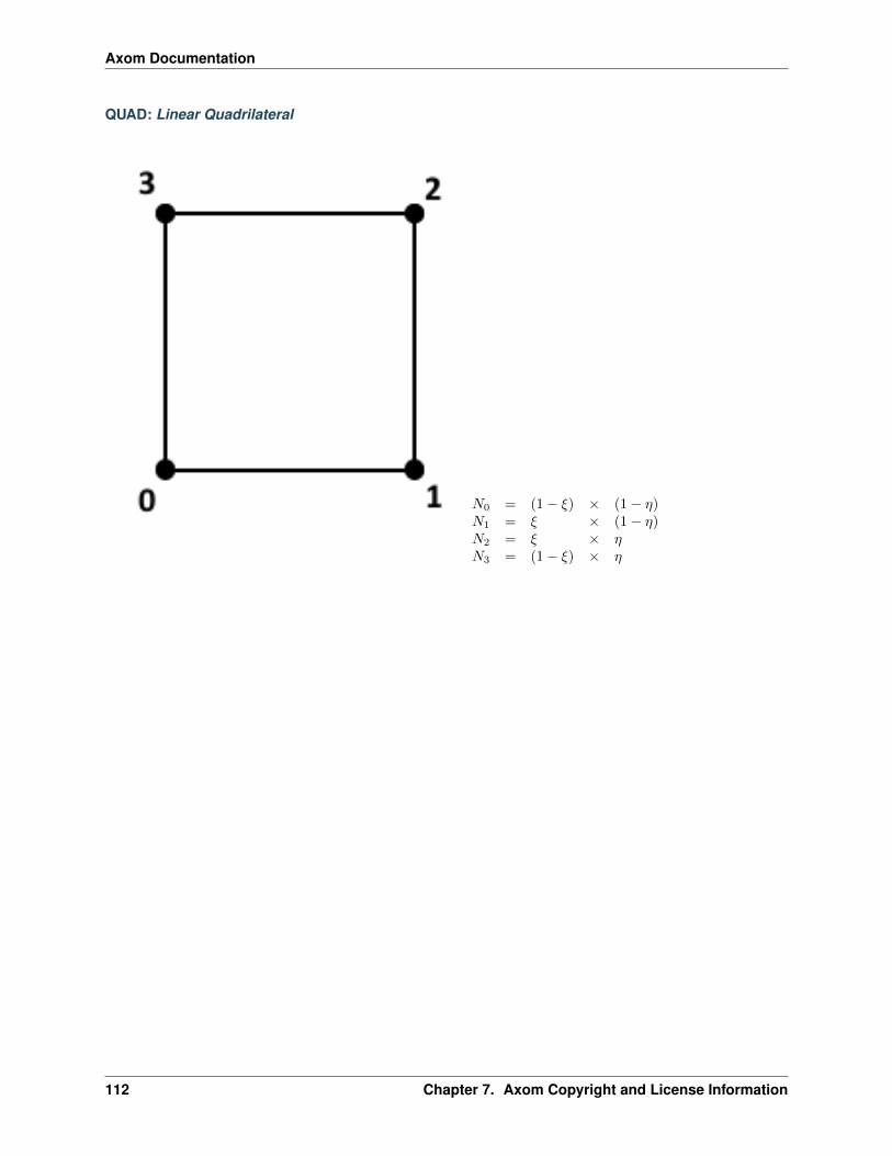
Axom Documentation

QUAD: Linear Quadrilateral

𝑁0 = (1 − 𝜉) × (1 − 𝜂)𝑁1 = 𝜉 × (1 − 𝜂)𝑁2 = 𝜉 × 𝜂𝑁3 = (1 − 𝜉) × 𝜂


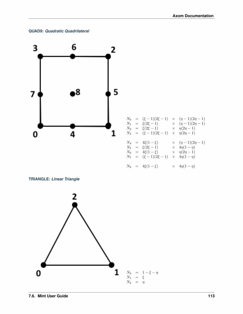
Axom Documentation

QUAD9: Quadratic Quadrilateral

𝑁0 = (𝜉 − 1)(2𝜉 − 1) × (𝜂 − 1)(2𝜂 − 1)𝑁1 = 𝜉(2𝜉 − 1) × (𝜂 − 1)(2𝜂 − 1)𝑁2 = 𝜉(2𝜉 − 1) × 𝜂(2𝜂 − 1)𝑁3 = (𝜉 − 1)(2𝜉 − 1) × 𝜂(2𝜂 − 1)

𝑁4 = 4𝜉(1 − 𝜉) × (𝜂 − 1)(2𝜂 − 1)𝑁5 = 𝜉(2𝜉 − 1) × 4𝜂(1 − 𝜂)𝑁6 = 4𝜉(1 − 𝜉) × 𝜂(2𝜂 − 1)𝑁7 = (𝜉 − 1)(2𝜉 − 1) × 4𝜂(1 − 𝜂)

𝑁8 = 4𝜉(1 − 𝜉) × 4𝜂(1 − 𝜂)

TRIANGLE: Linear Triangle

𝑁0 = 1 − 𝜉 − 𝜂𝑁1 = 𝜉𝑁2 = 𝜂


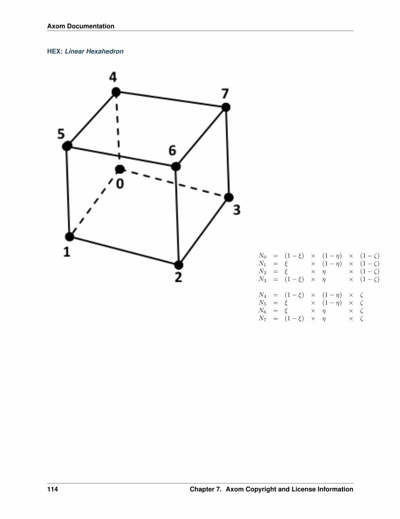
Axom Documentation

HEX: Linear Hexahedron

𝑁0 = (1 − 𝜉) × (1 − 𝜂) × (1 − 𝜁)𝑁1 = 𝜉 × (1 − 𝜂) × (1 − 𝜁)𝑁2 = 𝜉 × 𝜂 × (1 − 𝜁)𝑁3 = (1 − 𝜉) × 𝜂 × (1 − 𝜁)

𝑁4 = (1 − 𝜉) × (1 − 𝜂) × 𝜁𝑁5 = 𝜉 × (1 − 𝜂) × 𝜁𝑁6 = 𝜉 × 𝜂 × 𝜁𝑁7 = (1 − 𝜉) × 𝜂 × 𝜁


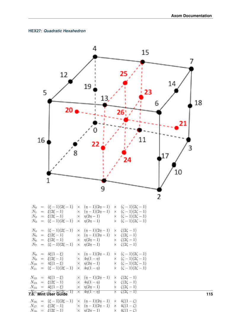
Axom Documentation

HEX27: Quadratic Hexahedron

𝑁0 = (𝜉 − 1)(2𝜉 − 1) × (𝜂 − 1)(2𝜂 − 1) × (𝜁 − 1)(2𝜁 − 1)𝑁1 = 𝜉(2𝜉 − 1) × (𝜂 − 1)(2𝜂 − 1) × (𝜁 − 1)(2𝜁 − 1)𝑁2 = 𝜉(2𝜉 − 1) × 𝜂(2𝜂 − 1) × (𝜁 − 1)(2𝜁 − 1)𝑁3 = (𝜉 − 1)(2𝜉 − 1) × 𝜂(2𝜂 − 1) × (𝜁 − 1)(2𝜁 − 1)

𝑁4 = (𝜉 − 1)(2𝜉 − 1) × (𝜂 − 1)(2𝜂 − 1) × 𝜁(2𝜁 − 1)𝑁5 = 𝜉(2𝜉 − 1) × (𝜂 − 1)(2𝜂 − 1) × 𝜁(2𝜁 − 1)𝑁6 = 𝜉(2𝜉 − 1) × 𝜂(2𝜂 − 1) × 𝜁(2𝜁 − 1)𝑁7 = (𝜉 − 1)(2𝜉 − 1) × 𝜂(2𝜂 − 1) × 𝜁(2𝜁 − 1)

𝑁8 = 4𝜉(1 − 𝜉) × (𝜂 − 1)(2𝜂 − 1) × (𝜁 − 1)(2𝜁 − 1)𝑁9 = 𝜉(2𝜉 − 1) × 4𝜂(1 − 𝜂) × (𝜁 − 1)(2𝜁 − 1)𝑁10 = 4𝜉(1 − 𝜉) × 𝜂(2𝜂 − 1) × (𝜁 − 1)(2𝜁 − 1)𝑁11 = (𝜉 − 1)(2𝜉 − 1) × 4𝜂(1 − 𝜂) × (𝜁 − 1)(2𝜁 − 1)

𝑁12 = 4𝜉(1 − 𝜉) × (𝜂 − 1)(2𝜂 − 1) × 𝜁(2𝜁 − 1)𝑁13 = 𝜉(2𝜉 − 1) × 4𝜂(1 − 𝜂) × 𝜁(2𝜁 − 1)𝑁14 = 4𝜉(1 − 𝜉) × 𝜂(2𝜂 − 1) × 𝜁(2𝜁 − 1)𝑁15 = (𝜉 − 1)(2𝜉 − 1) × 4𝜂(1 − 𝜂) × 𝜁(2𝜁 − 1)

𝑁16 = (𝜉 − 1)(2𝜉 − 1) × (𝜂 − 1)(2𝜂 − 1) × 4𝜁(1 − 𝜁)𝑁17 = 𝜉(2𝜉 − 1) × (𝜂 − 1)(2𝜂 − 1) × 4𝜁(1 − 𝜁)𝑁18 = 𝜉(2𝜉 − 1) × 𝜂(2𝜂 − 1) × 4𝜁(1 − 𝜁)𝑁19 = (𝜉 − 1)(2𝜉 − 1) × 𝜂(2𝜂 − 1) × 4𝜁(1 − 𝜁)

𝑁20 = (𝜉 − 1)(2𝜉 − 1) × 4𝜂(1 − 𝜂) × 4𝜁(1 − 𝜁)𝑁21 = 𝜉(2𝜉 − 1) × 4𝜂(1 − 𝜂) × 4𝜁(1 − 𝜁)𝑁22 = 4𝜉(1 − 𝜉) × (𝜂 − 1)(2𝜂 − 1) × 4𝜁(1 − 𝜁)𝑁23 = 4𝜉(1 − 𝜉) × 𝜂(2𝜂 − 1) × 4𝜁(1 − 𝜁)𝑁24 = 4𝜉(1 − 𝜉) × 4𝜂(1 − 𝜂) × (𝜁 − 1)(2𝜁 − 1)𝑁25 = 4𝜉(1 − 𝜉) × 4𝜂(1 − 𝜂) × 𝜁(2𝜁 − 1)

𝑁26 = 4𝜉(1 − 𝜉) × 4𝜂(1 − 𝜂) × 4𝜁(1 − 𝜁)


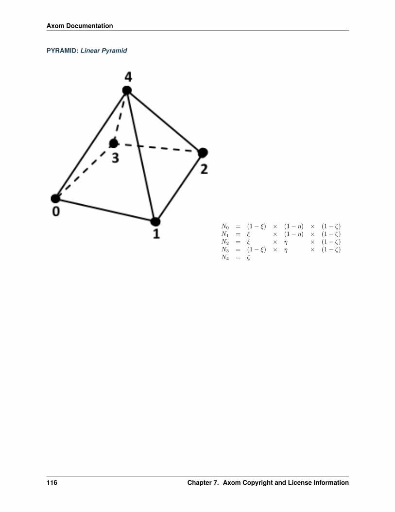
Axom Documentation

PYRAMID: Linear Pyramid

𝑁0 = (1 − 𝜉) × (1 − 𝜂) × (1 − 𝜁)𝑁1 = 𝜉 × (1 − 𝜂) × (1 − 𝜁)𝑁2 = 𝜉 × 𝜂 × (1 − 𝜁)𝑁3 = (1 − 𝜉) × 𝜂 × (1 − 𝜁)𝑁4 = 𝜁


Axom Documentation

PRISM: Linear Prism/Wedge

𝑁0 = (1 − 𝜉) − 𝜂 × (1 − 𝜁)𝑁1 = 𝜉 × (1 − 𝜁)𝑁2 = 𝜂 × (1 − 𝜁)𝑁3 = (1 − 𝜉) − 𝜂 × 𝜁𝑁4 = 𝜉 × 𝜁𝑁5 = 𝜂 × 𝜁

Add a New Lagrange Element


Isoparametric Mapping


Quadratures

Warning: Support for Quadratures in Mint is under development.

Add a New Finite Element Basis



Axom Documentation

Tutorial

The Tutorial section consists of simple examples and code snippets that illustrate how to use Mint’s core classesand functions to construct and operate on the various supported Mesh Types. The examples presented herein aimto illustrate specific Mint concepts and capabilities in a structured and simple format. To quickly learn basic Mintconcepts and capabilities through an illustrative walk-through of a complete working code example, see the GettingStarted with Mint section. Additional code examples, based on Mint mini-apps, are provided in the Examples section.For thorough documentation of the interfaces of the various classes and functions in Mint, developers are advised toconsult the Mint Doxygen API Documentation, in conjunction with this Tutorial.

Create a Uniform Mesh

A Uniform Mesh is relatively the simplest Structured Mesh type, but also, the most restrictive mesh out of all MeshTypes. The constituent Nodes of the Uniform Mesh are uniformly spaced along each axis on a regular lattice. Conse-quently, a Uniform Mesh can be easily constructed by simply specifying the spatial extents of the domain and desireddimensions, e.g. the number of Nodes along each dimension.

For example, a 50×50 Uniform Mesh, defined on a bounded domain given by the interval ℐ : [−5.0, 5.0]× [−5.0, 5.0],can be easily constructed as follows:

1 const double lo[] = -5.0, -5.0;2 const double hi[] = 5.0, 5.0;3 mint::UniformMesh mesh(lo, hi, 50, 50);

The resulting mesh is depicted in Fig. 7.22.

Create a Rectilinear Mesh

A Rectilinear Mesh, also called a product mesh, is similar to a Uniform Mesh. However, the constituent Nodes ofa Rectilinear Mesh are not uniformly spaced. The spacing between adjacent Nodes can vary arbitrarily along eachaxis, but the Topology of the mesh remains a regular Structured Mesh Topology. To allow for this flexibility, thecoordinates of the Nodes along each axis are explicitly stored in separate arrays, i.e. 𝑥, 𝑦 and 𝑧, for each coordinateaxis respectively.

The following code snippet illustrates how to construct a 25 × 25 Rectilinear Mesh where the spacing of the Nodesgrows according to an exponential stretching function along the 𝑥 and 𝑦 axis respectively. The resulting mesh isdepicted in Fig. 7.23.

1 constexpr double beta = 0.1;2 const double expbeta = exp(beta);3 const double invf = 1 / (expbeta - 1.0);4

5 // construct a N x N rectilinear mesh6 constexpr axom::IndexType N = 25;7 mint::RectilinearMesh mesh(N, N);8 double* x = mesh.getCoordinateArray(mint::X_COORDINATE);9 double* y = mesh.getCoordinateArray(mint::Y_COORDINATE);

10

11 // fill the coordinates along each axis12 x[0] = y[0] = 0.0;13 for(int i = 1; i < N; ++i)14 15 const double delta = (exp(i * beta) - 1.0) * invf;16 x[i] = x[i - 1] + delta;




Axom Documentation

Fig. 7.22: Resulting Uniform Mesh.


Axom Documentation


17 y[i] = y[i - 1] + delta;18

Fig. 7.23: Resulting Rectilinear Mesh.

Create a Curvilinear Mesh

A Curvilinear Mesh, also called a body-fitted mesh, is the most general of the Structured Mesh types. Similar to theUniform Mesh and Rectilinear Mesh types, a Curvilinear Mesh also has regular Structured Mesh Topology. However,the coordinates of the Nodes comprising a Curvilinear Mesh are defined explicitly, enabling the use of a StructuredMesh discretization with more general geometric domains, i.e., the domain may not be necessarily Cartesian. Conse-quently, the coordinates of the Nodes are specified explicitly in separate arrays, 𝑥, 𝑦, and 𝑧.

The following code snippet illustrates how to construct a 25 × 25 Curvilinear Mesh. The coordinates of the Nodesfollow from the equation of a cylinder with a radius of 2.5. The resulting mesh is depicted in Fig. 7.24.

1 constexpr double R = 2.5;2 constexpr double M = (2 * M_PI) / 50.0;3 constexpr double h = 0.5;4 constexpr axom::IndexType N = 25;



Axom Documentation


5

6 // construct the curvilinear mesh object7 mint::CurvilinearMesh mesh(N, N);8

9 // get a handle on the coordinate arrays10 double* x = mesh.getCoordinateArray(mint::X_COORDINATE);11 double* y = mesh.getCoordinateArray(mint::Y_COORDINATE);12

13 // fill the coordinates of the curvilinear mesh14 const axom::IndexType jp = mesh.nodeJp();15 for(axom::IndexType j = 0; j < N; ++j)16 17 const axom::IndexType j_offset = j * jp;18

19 for(axom::IndexType i = 0; i < N; ++i)20 21 const axom::IndexType nodeIdx = i + j_offset;22

23 const double xx = h * i;24 const double yy = h * j;25 const double alpha = yy + R;26 const double beta = xx * M;27

28 x[nodeIdx] = alpha * cos(beta);29 y[nodeIdx] = alpha * sin(beta);30 // END for all i31

32 // END for all j

Create an Unstructured Mesh

An Unstructured Mesh with Single Cell Type Topology has both explicit Topology and Geometry. However, the celltype that the mesh stores is known a priori, allowing for an optimized underlying Mesh Representation, compared tothe more general Mixed Cell Type Topology Mesh Representation.

Since both Geometry and Topology are explicit, an Unstructured Mesh is created by specifying:

1. the coordinates of the constituent Nodes, and

2. the Cells comprising the mesh, defined by the cell-to-node Connectivity

The following code snippet illustrates how to create the simple Unstructured Mesh depicted in Fig. 7.25.

1 constexpr int DIMENSION = 2;2 constexpr mint::CellType CELL_TYPE = mint::TRIANGLE;3

4 // Construct the mesh object5 mint::UnstructuredMesh<mint::SINGLE_SHAPE> mesh(DIMENSION, CELL_TYPE);6

7 // Append the mesh nodes8 const axom::IndexType n0 = mesh.appendNode(0.0, 0.0);9 const axom::IndexType n1 = mesh.appendNode(2.0, 0.0);

10 const axom::IndexType n2 = mesh.appendNode(1.0, 1.0);11 const axom::IndexType n3 = mesh.appendNode(3.5, 1.0);12 const axom::IndexType n4 = mesh.appendNode(2.5, 2.0);13 const axom::IndexType n5 = mesh.appendNode(5.0, 0.0);



Axom Documentation

Fig. 7.24: Resulting Curvilinear Mesh.

Fig. 7.25: Resulting Single Cell Type Topology Unstructured Mesh


Axom Documentation


14

15 // Append mesh cells16 const axom::IndexType c0[] = n1, n3, n2;17 const axom::IndexType c1[] = n2, n0, n1;18 const axom::IndexType c2[] = n3, n4, n2;19 const axom::IndexType c3[] = n1, n5, n3;20

21 mesh.appendCell(c0);22 mesh.appendCell(c1);23 mesh.appendCell(c2);24 mesh.appendCell(c3);

An Unstructured Mesh is represented by the mint::UnstructuredMesh template class. The template argu-ment of the class, mint::SINGLE_SHAPE indicates the mesh has Single Cell Type Topology. The two argu-ments to the class constructor correspond to the problem dimension and cell type, which in this case, is 2 andmint::TRIANGLE respectively. Once the mesh is constructed, the Nodes and Cells are appended to the meshby calls to the appendNode() and appendCell() methods respectively. The resulting mesh is shown in Fig.7.25.

Tip: The storage for the mint::UstructuredMesh will grow dynamically as new Nodes and Cells are appendedon the mesh. However, reallocations tend to be costly operations. For best performance, it is advised the node capacityand cell capacity for the mesh are specified in the constructor if known a priori. Consult the Mint Doxygen APIDocumentation for more details.

Create a Mixed Unstructured Mesh

Compared to the Single Cell Type Topology Unstructured Mesh, a Mixed Cell Type Topology Unstructured Mesh hasalso explicit Topology and Geometry. However, the cell type is not fixed. Notably, the mesh can store different CellTypes, e.g. triangles and quads, as shown in the simple 2D mesh depicted in Fig. 7.26.

Fig. 7.26: Sample Mixed Cell Type Topology Unstructured Mesh

As with the Single Cell Type Topology Unstructured Mesh, a Mixed Cell Type Topology Unstructured Mesh is createdby specifying:

1. the coordinates of the constituent Nodes, and

2. the Cells comprising the mesh, defined by the cell-to-node Connectivity




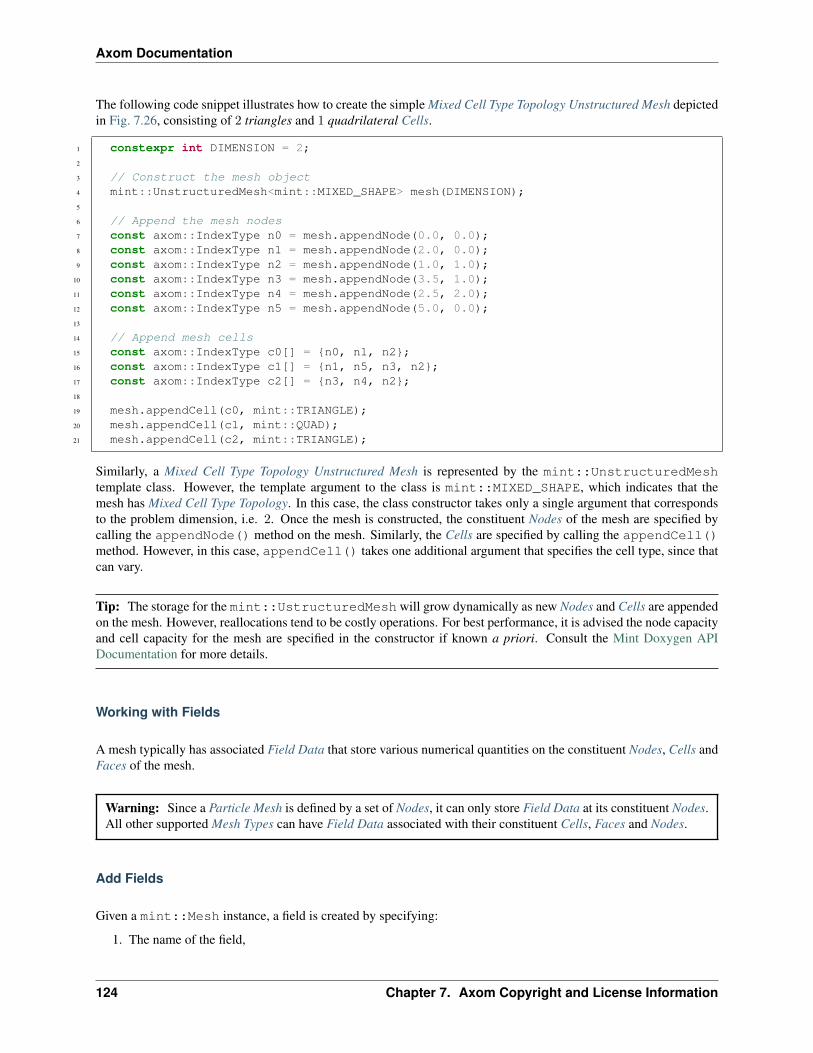
Axom Documentation

The following code snippet illustrates how to create the simple Mixed Cell Type Topology Unstructured Mesh depictedin Fig. 7.26, consisting of 2 triangles and 1 quadrilateral Cells.

1 constexpr int DIMENSION = 2;2

3 // Construct the mesh object4 mint::UnstructuredMesh<mint::MIXED_SHAPE> mesh(DIMENSION);5

6 // Append the mesh nodes7 const axom::IndexType n0 = mesh.appendNode(0.0, 0.0);8 const axom::IndexType n1 = mesh.appendNode(2.0, 0.0);9 const axom::IndexType n2 = mesh.appendNode(1.0, 1.0);

10 const axom::IndexType n3 = mesh.appendNode(3.5, 1.0);11 const axom::IndexType n4 = mesh.appendNode(2.5, 2.0);12 const axom::IndexType n5 = mesh.appendNode(5.0, 0.0);13

14 // Append mesh cells15 const axom::IndexType c0[] = n0, n1, n2;16 const axom::IndexType c1[] = n1, n5, n3, n2;17 const axom::IndexType c2[] = n3, n4, n2;18

19 mesh.appendCell(c0, mint::TRIANGLE);20 mesh.appendCell(c1, mint::QUAD);21 mesh.appendCell(c2, mint::TRIANGLE);

Similarly, a Mixed Cell Type Topology Unstructured Mesh is represented by the mint::UnstructuredMeshtemplate class. However, the template argument to the class is mint::MIXED_SHAPE, which indicates that themesh has Mixed Cell Type Topology. In this case, the class constructor takes only a single argument that correspondsto the problem dimension, i.e. 2. Once the mesh is constructed, the constituent Nodes of the mesh are specified bycalling the appendNode() method on the mesh. Similarly, the Cells are specified by calling the appendCell()method. However, in this case, appendCell() takes one additional argument that specifies the cell type, since thatcan vary.

Tip: The storage for the mint::UstructuredMesh will grow dynamically as new Nodes and Cells are appendedon the mesh. However, reallocations tend to be costly operations. For best performance, it is advised the node capacityand cell capacity for the mesh are specified in the constructor if known a priori. Consult the Mint Doxygen APIDocumentation for more details.

Working with Fields

A mesh typically has associated Field Data that store various numerical quantities on the constituent Nodes, Cells andFaces of the mesh.

Warning: Since a Particle Mesh is defined by a set of Nodes, it can only store Field Data at its constituent Nodes.All other supported Mesh Types can have Field Data associated with their constituent Cells, Faces and Nodes.

Add Fields

Given a mint::Mesh instance, a field is created by specifying:

1. The name of the field,




Axom Documentation

2. The field association, i.e. centering, and

3. Optionally, the number of components of the field, required if the field is not a scalar quantity.

For example, the following code snippet creates the scalar density field, den, stored at the cell centers, and the vectorvelocity field, vel, stored at the Nodes:

1 double* den = mesh->createField<double>("den", mint::CELL_CENTERED);2 double* vel = mesh->createField<double>("vel", mint::NODE_CENTERED, 3);

Note: If Sidre is used as the backend Mesh Storage Management substrate, createField() will populate theSidre tree hierarchy accordingly. See Using Sidre for more information.

• Note, the template argument to the createField()method indicates the underlying field type, e.g. double,int , etc. In this case, both fields are of double field type.

• The name of the field is specified by the first required argument to the createField() call.

• The field association, is specified by the second argument to the createField() call.

• A third, optional, argument may be specified to indicate the number of components of the corresponding field.In this case, since vel is a vector quantity the number of components must be explicitly specified.

• The createField() method returns a raw pointer to the data corresponding to the new field, which can beused by the application.

Note: Absence of the third argument when calling createField() indicates that the number of components ofthe field defaults to 1 and thereby the field is assumed to be a scalar quantity.

Request Fields by Name

Specific, existing fields can be requested by calling getFieldPtr() on the target mesh as follows:

1 double* den = mesh->getFieldPtr<double>("den", mint::CELL_CENTERED);2

3 axom::IndexType nc = -1; // number of components4 double* vel = mesh->getFieldPtr<double>("vel", mint::NODE_CENTERED, nc);

• As with the createField() method, the template argument indicates the underlying field type, e.g.double, int , etc.

• The first argument specifies the name of the requested field

• The second argument specifies the corresponding association of the requested field.

• The third argument is optional and it can be used to get back the number of components of the field, i.e. if thefield is not a scalar quantity.

Note: Calls to getFieldPtr() assume that the caller knows a priori the:

• Field name,

• Field association, i.e. centering, and

• The underlying field type, e.g. double, int, etc.




Axom Documentation

Check Fields

An application can also check if a field exists by calling hasField() on the mesh, which takes as arguments thefield name and corresponding field association as follows:

1 const bool hasDen = mesh->hasField("den", mint::CELL_CENTERED);2 const bool hasVel = mesh->hasField("vel", mint::NODE_CENTERED);

The hasField() method returns true or false indicating whether a given field is defined on the mesh.

Remove Fields

A field can be removed from a mesh by calling removeField() on the target mesh, which takes as arguments thefield name and corresponding field association as follows:

1 bool isRemoved = mesh->removeField("den", mint::CELL_CENTERED);

The removeField() method returns true or false indicating whether the corresponding field was removedsuccessfully from the mesh.

Query Fields

In some cases, an application may not always know a priori the name or type of the field, or, we may want to write afunction to process all fields, regardless of their type.

The following code snippet illustrates how to do that:

1 const mint::FieldData* fieldData = mesh->getFieldData(FIELD_ASSOCIATION);2

3 const int numFields = fieldData->getNumFields();4 for(int ifield = 0; ifield < numFields; ++ifield)5 6 const mint::Field* field = fieldData->getField(ifield);7

8 const std::string& fieldName = field->getName();9 axom::IndexType numTuples = field->getNumTuples();

10 axom::IndexType numComponents = field->getNumComponents();11

12 std::cout << "field name: " << fieldName << std::endl;13 std::cout << "numTuples: " << numTuples << std::endl;14 std::cout << "numComponents: " << numComponents << std::endl;15

16 if(field->getType() == mint::DOUBLE_FIELD_TYPE)17 18 double* data = mesh->getFieldPtr<double>(fieldName, FIELD_ASSOCIATION);19 data[0] = 42.0;20 // process double precision floating point data21 // ...22 23 else if(field->getType() == mint::INT32_FIELD_TYPE)24 25 int* data = mesh->getFieldPtr<int>(fieldName, FIELD_ASSOCIATION);26 data[0] = 42;27 // process integral data



Axom Documentation


28 // ...29 30 // ...31

32 // END for all fields

• The mint::FieldData instance obtained by calling getFieldData() on the target mesh holds all thefields with a field association given by FIELD_ASSOCIATION.

• The total number of fields can be obtained by calling getNumFields() on the mint::FieldData in-stance, which allows looping over the fields with a simple for loop.

• Within the loop, a pointer to a mint::Field instance, corresponding to a particular field, can be requestedby calling getField() on the mint::FieldData instance, which takes the field index, ifield, as anargument.

• Given the pointer to a mint::Field instance, an application can query the following field metadata:

– The field name, by calling getName,

– The number of tuples of the field, by calling getNumTuples()

– The number of components of the field, by calling getNumComponents()

– The underlying field type by calling getType()

• Given the above metadata, the application can then obtain a pointer to the raw field data by callinggetFieldPtr() on the target mesh, as shown in the code snippet above.

Using External Storage

A Mint mesh may also be constructed from External Storage. In this case, the application holds buffers that describethe constituent Geometry, Topology and Field Data of the mesh, which are wrapped in Mint for further processing.

The following code snippet illustrates how to use External Storage using the Single Cell Type Topology UnstructuredMesh used to demonstrate how to Create an Unstructured Mesh with Native Storage:

1 constexpr axom::IndexType NUM_NODES = 6;2 constexpr axom::IndexType NUM_CELLS = 4;3

4 // application buffers5 double x[] = 0.0, 2.0, 1.0, 3.5, 2.5, 5.0;6 double y[] = 0.0, 0.0, 1.0, 1.0, 2.0, 0.0;7

8 axom::IndexType cell_connectivity[] = 9 1,

10 3,11 2, // c012 2,13 0,14 1, // c115 3,16 4,17 2, // c218 1,19 5,20 3 // c321 ;



Axom Documentation


22

23 // cell-centered density field values24 double den[] = 0.5, 1.2, 2.5, 0.9;25

26 // construct mesh object with external buffers27 using MeshType = mint::UnstructuredMesh<mint::SINGLE_SHAPE>;28 MeshType* mesh =29 new MeshType(mint::TRIANGLE, NUM_CELLS, cell_connectivity, NUM_NODES, x, y);30

31 // register external field32 mesh->createField<double>("den", mint::CELL_CENTERED, den);33

34 // output external mesh to vtk35 mint::write_vtk(mesh, "tutorial_external_mesh.vtk");36

37 // delete the mesh, doesn't touch application buffers38 delete mesh;39 mesh = nullptr;

• The application has the following buffers:

– x and y buffers to hold the coordinates of the Nodes

– cell_connectivity, which stores the cell-to-node connectivity

– den which holds a scalar density field defined over the constituent Cells of the mesh.

• The mesh is created by calling the mint::UnstructuredMesh class constructor, with the following argu-ments:

– The cell type, i.e, mint::TRIANGLE,

– The total number of cells, NUM_CELLS,

– The cell_connectivity which specifies the Topology of the Unstructured Mesh,

– The total number of nodes, NUM_NODES, and

– The x, y coordinate buffers that specify the Geometry of the Unstructured Mesh.

• The scalar density field is registered with Mint by calling the createField() method on the target meshinstance, as before, but also passing the raw pointer to the application buffer in a third argument.

Note: The other Mesh Types can be similarly constructed using External Storage by calling the appropriate construc-tor. Consult the Mint Doxygen API Documentation for more details.

The resulting mesh instance points to the application’s buffers. Mint may be used to process the data e.g., Output toVTK etc. The values of the data may also be modified, however the mesh cannot dynamically grow or shrink whenusing External Storage.

Warning: A mesh using External Storage may modify the values of the application data. However, the data isowned by the application that supplied the external buffers. Mint cannot reallocate external buffers to grow orshrink the the mesh. Once the mesh is deleted, the data remains persistent in the application buffers until it isdeleted by the application.



Axom Documentation

Using Sidre

Mint can also use Sidre as the underlying Mesh Storage Management substrate, thereby, facilitate the integration ofpackages or codes within the overarching WSC software ecosystem. Sidre is another component of the Axom Toolkitthat provides a centralized data management system that enables efficient coordination of data across the constituentpackages of a multi-physics application.

There are two primary operations a package/code may want to perform:

1. Create a new Mesh in Sidre so that it can be shared with other packages.

2. Import a Mesh from Sidre, presumably created by different package or code upstream, to operate on, e.g. evalu-ate a new field on the mesh, etc.

Code snippets illustrating these two operations are presented in the following sections using a simple UnstructuredMesh example. However, the basic concepts extend to all supported Mesh Types.

Note: To use Sidre with Mint, the Axom Toolkit must be compiled with Conduit support and Sidre must be enabled(default). Consult the Axom Quick Start Guide for the details on how to build the Axom Toolkit.

Create a new Mesh in Sidre

Creating a mesh using Sidre is very similar to creating a mesh that uses Native Storage. The key difference is thatwhen calling the mesh constructor, the target sidre::Group, that will consist of the mesh, must be specified.

Warning: The target sidre::Group supplied to the mesh constructor is expected to be empty.

The following code snippet illustrates this capability using the Single Cell Type Topology Unstructured Mesh used todemonstrate how to Create an Unstructured Mesh with Native Storage. The key differences in the code are highlightedbelow:

1 // create a Sidre Datastore to store the mesh2 sidre::DataStore ds;3 sidre::Group* group = ds.getRoot();4

5 // Construct the mesh object and populate the supplied Sidre Group6 mint::UnstructuredMesh<mint::SINGLE_SHAPE> mesh(2, mint::TRIANGLE, group);7

8 // Append the mesh nodes9 const axom::IndexType n0 = mesh.appendNode(0.0, 0.0);

10 const axom::IndexType n1 = mesh.appendNode(2.0, 0.0);11 const axom::IndexType n2 = mesh.appendNode(1.0, 1.0);12 const axom::IndexType n3 = mesh.appendNode(3.5, 1.0);13 const axom::IndexType n4 = mesh.appendNode(2.5, 2.0);14 const axom::IndexType n5 = mesh.appendNode(5.0, 0.0);15

16 // Append mesh cells17 const axom::IndexType c0[] = n1, n3, n2;18 const axom::IndexType c1[] = n2, n0, n1;19 const axom::IndexType c2[] = n3, n4, n2;20 const axom::IndexType c3[] = n1, n5, n3;21

22 mesh.appendCell(c0);




https://wci.llnl.gov/about-us/weapon-simulation-and-computing


../../../../../index.html


../../../../../index.html




../../../../../index.html


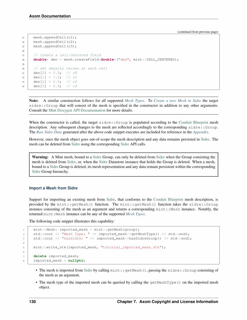
Axom Documentation


23 mesh.appendCell(c1);24 mesh.appendCell(c2);25 mesh.appendCell(c3);26

27 // create a cell-centered field28 double* den = mesh.createField<double>("den", mint::CELL_CENTERED);29

30 // set density values at each cell31 den[0] = 0.5; // c032 den[1] = 1.2; // c133 den[2] = 2.5; // c234 den[3] = 0.9; // c3

Note: A similar construction follows for all supported Mesh Types. To Create a new Mesh in Sidre the targetsidre::Group that will consist of the mesh is specified in the constructor in addition to any other arguments.Consult the Mint Doxygen API Documentation for more details.

When the constructor is called, the target sidre::Group is populated according to the Conduit Blueprint meshdescription. Any subsequent changes to the mesh are reflected accordingly to the corresponding sidre::Group.The Raw Sidre Data generated after the above code snippet executes are included for reference in the Appendix.

However, once the mesh object goes out-of-scope the mesh description and any data remains persisted in Sidre. Themesh can be deleted from Sidre using the corresponding Sidre API calls.

Warning: A Mint mesh, bound to a Sidre Group, can only be deleted from Sidre when the Group consisting themesh is deleted from Sidre, or, when the Sidre Datastore instance that holds the Group is deleted. When a mesh,bound to a Sidre Group is deleted, its mesh representation and any data remain persistent within the correspondingSidre Group hierarchy.

Import a Mesh from Sidre

Support for importing an existing mesh from Sidre, that conforms to the Conduit Blueprint mesh description, isprovided by the mint::getMesh() function. The mint::getMesh() function takes the sidre::Groupinstance consisting of the mesh as an argument and returns a corresponding mint::Mesh instance. Notably, thereturned mint:Mesh instance can be any of the supported Mesh Types.

The following code snippet illustrates this capability:

1 mint::Mesh* imported_mesh = mint::getMesh(group);2 std::cout << "Mesh Type: " << imported_mesh->getMeshType() << std::endl;3 std::cout << "hasSidre: " << imported_mesh->hasSidreGroup() << std::endl;4

5 mint::write_vtk(imported_mesh, "tutorial_imported_mesh.vtk");6

7 delete imported_mesh;8 imported_mesh = nullptr;

• The mesh is imported from Sidre by calling mint::getMesh(), passing the sidre::Group consisting ofthe mesh as an argument.

• The mesh type of the imported mesh can be queried by calling the getMeshType() on the imported meshobject.


















Axom Documentation

• Moreover, an application can check if the mesh is bound to a Sidre group by calling hasSidreGroup() onthe mesh.

• Once the mesh is imported, the application can operate on it, e.g. Output to VTK, etc., as illustrated in the abovecode snippet.

• Any subsequent changes to the mesh are reflected accordingly to the corresponding sidre::Group

However, once the mesh object goes out-of-scope the mesh description and any data remains persisted in Sidre. Themesh can be deleted from Sidre using the corresponding Sidre API calls.

Warning:

• When a Mint mesh bound to a Sidre Group is deleted, its mesh representation and any data remain persistentwithin the corresponding Sidre Group hierarchy.

• A Mint mesh, bound to a Sidre Group, is deleted from Sidre by deleting the corresponding Sidre Group, or,when the Sidre Datastore instance that holds the Group is deleted.

Node Traversal Functions

The Node Traversal Functions iterate over the constituent Nodes of the mesh and apply a user-supplied kerneloperation, often specified with a Lambda Expression. The Node Traversal Functions are implemented by themint::for_all_nodes() family of functions, which take an Execution Policy as the first template argument,and optionally, a second template argument to indicate the Execution Signature of the supplied kernel.

Note: If a second template argument is not specified, the default Execution Signature is set to xargs::index,which indicates that the supplied kernel takes a single argument corresponding to the index of the iteration space, inthis case the node index, nodeIdx.

Simple Loop Over Nodes

The following code snippet illustrates a simple loop over the Nodes of a 2D mesh that computes the velocity magnitude,vmag, given the corresponding velocity components, vx and vy.

1 const double* vx = mesh.getFieldPtr<double>("vx", mint::NODE_CENTERED);2 const double* vy = mesh.getFieldPtr<double>("vy", mint::NODE_CENTERED);3

4 double* vmag = mesh.getFieldPtr<double>("vmag", mint::NODE_CENTERED);5

6 mint::for_all_nodes<exec_policy>(7 &mesh,8 AXOM_LAMBDA(IndexType nodeIdx) 9 const double vx2 = vx[nodeIdx] * vx[nodeIdx];

10 const double vy2 = vy[nodeIdx] * vy[nodeIdx];11 vmag[nodeIdx] = sqrt(vx2 + vy2);12 );













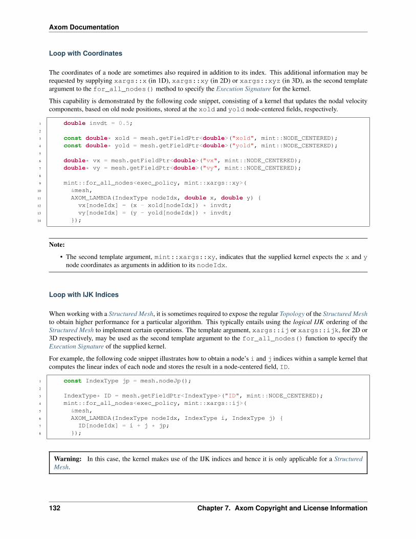
Axom Documentation

Loop with Coordinates

The coordinates of a node are sometimes also required in addition to its index. This additional information may berequested by supplying xargs::x (in 1D), xargs::xy (in 2D) or xargs::xyz (in 3D), as the second templateargument to the for_all_nodes() method to specify the Execution Signature for the kernel.

This capability is demonstrated by the following code snippet, consisting of a kernel that updates the nodal velocitycomponents, based on old node positions, stored at the xold and yold node-centered fields, respectively.

1 double invdt = 0.5;2

3 const double* xold = mesh.getFieldPtr<double>("xold", mint::NODE_CENTERED);4 const double* yold = mesh.getFieldPtr<double>("yold", mint::NODE_CENTERED);5

6 double* vx = mesh.getFieldPtr<double>("vx", mint::NODE_CENTERED);7 double* vy = mesh.getFieldPtr<double>("vy", mint::NODE_CENTERED);8

9 mint::for_all_nodes<exec_policy, mint::xargs::xy>(10 &mesh,11 AXOM_LAMBDA(IndexType nodeIdx, double x, double y) 12 vx[nodeIdx] = (x - xold[nodeIdx]) * invdt;13 vy[nodeIdx] = (y - yold[nodeIdx]) * invdt;14 );

Note:

• The second template argument, mint::xargs::xy, indicates that the supplied kernel expects the x and ynode coordinates as arguments in addition to its nodeIdx.

Loop with IJK Indices

When working with a Structured Mesh, it is sometimes required to expose the regular Topology of the Structured Meshto obtain higher performance for a particular algorithm. This typically entails using the logical IJK ordering of theStructured Mesh to implement certain operations. The template argument, xargs::ij or xargs::ijk, for 2D or3D respectively, may be used as the second template argument to the for_all_nodes() function to specify theExecution Signature of the supplied kernel.

For example, the following code snippet illustrates how to obtain a node’s i and j indices within a sample kernel thatcomputes the linear index of each node and stores the result in a node-centered field, ID.

1 const IndexType jp = mesh.nodeJp();2

3 IndexType* ID = mesh.getFieldPtr<IndexType>("ID", mint::NODE_CENTERED);4 mint::for_all_nodes<exec_policy, mint::xargs::ij>(5 &mesh,6 AXOM_LAMBDA(IndexType nodeIdx, IndexType i, IndexType j) 7 ID[nodeIdx] = i + j * jp;8 );

Warning: In this case, the kernel makes use of the IJK indices and hence it is only applicable for a StructuredMesh.


Axom Documentation

Cell Traversal Functions

The Cell Traversal Functions iterate over the constituent Cells of the mesh and apply a user-supplied kerneloperation, often specified with a Lambda Expression. The Cell Traversal Functions are implemented by themint::for_all_cells() family of functions, which take an Execution Policy as the first template argument,and optionally, a second template argument to indicate the Execution Signature of the supplied kernel.

Note: If a second template argument is not specified, the default Execution Signature is set to xargs::index,which indicates that the supplied kernel takes a single argument corresponding to the index of the iteration space, inthis case the cell index, cellIdx.

Simple Loop Over Cells

The following code snippet illustrates a simple loop over the constituent Cells of the mesh that computes the celldensity (den), given corresponding mass (mass) and volume (vol) quantities.

1 const double* mass = mesh.getFieldPtr<double>("mass", mint::CELL_CENTERED);2 const double* vol = mesh.getFieldPtr<double>("vol", mint::CELL_CENTERED);3

4 double* den = mesh.getFieldPtr<double>("den", mint::CELL_CENTERED);5

6 mint::for_all_cells<exec_policy>(7 &mesh,8 AXOM_LAMBDA(IndexType cellIdx) 9 den[cellIdx] = mass[cellIdx] / vol[cellIdx];

10 );

Loop with Node IDs

Certain operations may require the IDs of the constituent cell Nodes for some calculation. The template argument,xargs::nodeids, may be used as the second template argument to the for_all_cells() function to specifythe Execution Signature for the kernel. The xargs::nodeids indicates that the supplied kernel also takes the theIDs of the constituent cell Nodes as an argument.

This feature is demonstrated with the following code snippet, which averages the node-centered velocity componentsto corresponding cell-centered fields:


4 double* cell_vx = mesh.getFieldPtr<double>("cell_vx", mint::CELL_CENTERED);5 double* cell_vy = mesh.getFieldPtr<double>("cell_vy", mint::CELL_CENTERED);6

7 mint::for_all_cells<exec_policy, mint::xargs::nodeids>(8 &mesh,9 AXOM_LAMBDA(IndexType cellIdx, const IndexType* nodeIDs, IndexType N)

10 // sum nodal contributions11 cell_vx[cellIdx] = 0.0;12 cell_vy[cellIdx] = 0.0;13 for(IndexType inode = 0; inode < N; ++inode)14 15 cell_vx[cellIdx] += vx[nodeIDs[inode]];




Axom Documentation


16 cell_vy[cellIdx] += vy[nodeIDs[inode]];17 // END for all cell nodes18

19 // average at the cell center20 const double invf = 1.0 / static_cast<double>(N);21 cell_vx[cellIdx] *= invf;22 cell_vy[cellIdx] *= invf;23 );

Note:

• xargs::nodeids indicates that the specified kernel takes three arguments:

– cellIdx, the ID of the cell,

– nodeIDs, an array of the constituent node IDs, and

– N, the number of Nodes for the given cell.


The coordinates of the constituent cell Nodes are often required in some calculations. A cell’s node coordinates maybe supplied to the specified kernel as an argument using xargs::coords as the second template argument to thefor_all_cells() function, to specify the Execution Signature of the supplied kernel.

This feature is demonstrated with the following code snippet, which computes the cell centroid by averaging thecoordinates of the constituent cell Nodes:

Note: Since this kernel does not use the node IDs, the argument to the kernel is annotated using theAXOM_UNUSED_PARAM macro to silence compiler warnings.

1 double* xc = mesh.getFieldPtr<double>("xc", mint::CELL_CENTERED);2 double* yc = mesh.getFieldPtr<double>("yc", mint::CELL_CENTERED);3

4 mint::for_all_cells<exec_policy, mint::xargs::coords>(5 &mesh,6 AXOM_LAMBDA(IndexType cellIdx,7 const numerics::Matrix<double>& coords,8 const IndexType* AXOM_UNUSED_PARAM(nodeIdx)) 9 // sum nodal coordinates

10 double xsum = 0.0;11 double ysum = 0.0;12 const int numNodes = coords.getNumColumns();13 for(int inode = 0; inode < numNodes; ++inode)14 15 const double* node = coords.getColumn(inode);16 xsum += node[mint::X_COORDINATE];17 ysum += node[mint::Y_COORDINATE];18 // end for all cell nodes19

20 // compute centroid by averaging nodal coordinates21 const double invf = 1.0 / static_cast<double>(numNodes);22 xc[cellIdx] = xsum * invf;



Axom Documentation


23 yc[cellIdx] = ysum * invf;24 );

Note:

• xargs::coords indicates that the specified kernel takes the following arguments:


– coords, a matrix that stores the cell coordinates, such that:

* The number of rows corresponds to the problem dimension, and,

* The number of columns corresponds to the number of nodes.

* The 𝑖𝑡ℎ column vector of the matrix stores the coordinates of the 𝑖𝑡ℎ node.

– nodeIdx array of corresponding node IDs.

Loop with Face IDs

The IDs of the constituent cell Faces are sometimes needed to access the corresponding face-centered quantities forcertain operations. The face IDs can be obtained using xargs::faceids as the second template argument to thefor_all_faces() function, to specify the Execution Signature of the supplied kernel.

This feature is demonstrated with the following code snippet, which computes the perimeter of each cell by summingthe pre-computed face areas:

1 const double* area = mesh.getFieldPtr<double>("area", mint::FACE_CENTERED);2 double* perimeter =3 mesh.getFieldPtr<double>("perimeter", mint::CELL_CENTERED);4

5 mint::for_all_cells<exec_policy, mint::xargs::faceids>(6 &mesh,7 AXOM_LAMBDA(IndexType cellIdx, const IndexType* faceIDs, IndexType N) 8 perimeter[cellIdx] = 0.0;9 for(IndexType iface = 0; iface < N; ++iface)

10 11 perimeter[cellIdx] += area[faceIDs[iface]];12 13 );

Note:

• xargs::faceids indicates that the specified kernel takes the following arguments:


– faceIDs, an array of the constituent face IDs, and,

– N, the number of Faces for the given cell.


Axom Documentation

Loop with IJK Indices

As with the Node Traversal Functions, when working with a Structured Mesh, it is sometimes required to exposethe regular Topology of the Structured Mesh to obtain higher performance for a particular algorithm. This typi-cally entails using the logical IJK ordering of the Structured Mesh to implement certain operations. The templateargument, xargs::ij (in 2D) or xargs::ijk (in 3D) may be used as the second template argument to thefor_all_cells() function, to specify the Execution Signature of the supplied kernel.

For example, the following code snippet illustrates to obtain a cell’s i and j indices within a kernel that computes thelinear index of each cell and stores the result in a cell-centered field, ID.

1 const IndexType jp = mesh.cellJp();2

3 IndexType* ID = mesh.getFieldPtr<IndexType>("ID", mint::CELL_CENTERED);4 mint::for_all_cells<exec_policy, mint::xargs::ij>(5 &mesh,6 AXOM_LAMBDA(IndexType cellIdx, IndexType i, IndexType j) 7 ID[cellIdx] = i + j * jp;8 );

Warning: In this case, the kernel makes use of the IJK indices and hence it is only applicable for a StructuredMesh.

Face Traversal Functions

The Face Traversal Functions functions iterate over the constituent Faces of the mesh and apply a user-suppliedkernel operation, often specified with a Lambda Expression. The Face Traversal Functions are implemented by themint::for_all_faces() family of functions. which take an Execution Policy as the first template argument,and optionally, a second template argument to indicate the Execution Signature of the supplied kernel.

Note: If a second template argument is not specified, the default Execution Signature is set to xargs::index,which indicates that the supplied kernel takes a single argument corresponding to the index of the iteration space, inthis case the face index, faceIdx.

Simple Loop Over Faces

The following code snippet illustrates a simple loop over the constituent Faces of a 2D mesh that computes an inter-polated face-centered quantity (temp) based on pre-computed interpolation coefficients t1 , t2 and w.

1 const double* t1 = mesh.getFieldPtr<double>("t1", mint::FACE_CENTERED);2 const double* t2 = mesh.getFieldPtr<double>("t2", mint::FACE_CENTERED);3 const double* w = mesh.getFieldPtr<double>("w", mint::FACE_CENTERED);4

5 double* temp = mesh.getFieldPtr<double>("temp", mint::FACE_CENTERED);6 mint::for_all_faces<exec_policy>(7 &mesh,8 AXOM_LAMBDA(IndexType faceIdx) 9 const double wf = w[faceIdx];

10 const double a = t1[faceIdx];11 const double b = t2[faceIdx];




Axom Documentation


12

13 temp[faceIdx] = wf * a + (1. - wf) * b;14 );

Loop with Node IDs

The IDs of the constituent face Nodes are sometimes needed to access associated node-centered data for certaincalculations. The template argument, xargs::nodeids, may be used as the second template argument to thefor_all_faces() function to specify the Execution Signature of the supplied kernel. The xargs::nodeidstemplate argument indicates that the supplied kernel also takes the IDs of the constituent face Nodes as an argument.

This feature is demonstrated with the following code snippet which averages the node-centered velocity componentsto corresponding face-centered quantities:


4 double* face_vx = mesh.getFieldPtr<double>("face_vx", mint::FACE_CENTERED);5 double* face_vy = mesh.getFieldPtr<double>("face_vy", mint::FACE_CENTERED);6

7 mint::for_all_faces<exec_policy, mint::xargs::nodeids>(8 &mesh,9 AXOM_LAMBDA(IndexType faceIdx, const IndexType* nodeIDs, IndexType N)

10 // sum constituent face node contributions11 face_vx[faceIdx] = 0.0;12 face_vy[faceIdx] = 0.0;13 for(int inode = 0; inode < N; ++inode)14 15 face_vx[faceIdx] += vx[nodeIDs[inode]];16 face_vy[faceIdx] += vy[nodeIDs[inode]];17 // END for all face nodes18

19 // average20 const double invf = 1.0 / static_cast<double>(N);21 face_vx[faceIdx] *= invf;22 face_vy[faceIdx] *= invf;23 );

Note:

• xargs::nodeids indicates that the specified kernel takes three arguments:

– faceIdx, the ID of the cell,

– nodeIDs, an array of the constituent node IDs, and

– N, the number of Nodes for the corresponding face.


The coordinates of the constituent face Nodes are often required in some calculations. The constituent face nodecoordinates may be supplied to the specified kernel as an argument using xargs::coords as the second templateargument to the for_all_faces() function, to specify the Execution Signature of the supplied kernel.


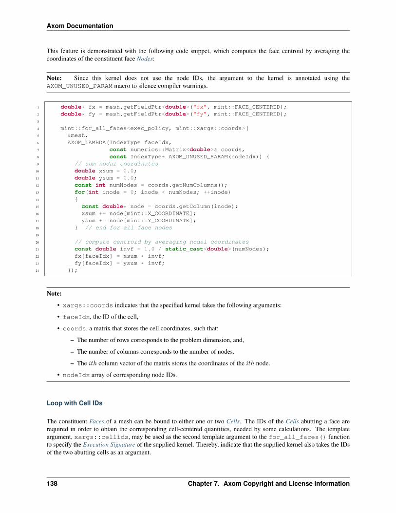
Axom Documentation

This feature is demonstrated with the following code snippet, which computes the face centroid by averaging thecoordinates of the constituent face Nodes:

Note: Since this kernel does not use the node IDs, the argument to the kernel is annotated using theAXOM_UNUSED_PARAM macro to silence compiler warnings.

1 double* fx = mesh.getFieldPtr<double>("fx", mint::FACE_CENTERED);2 double* fy = mesh.getFieldPtr<double>("fy", mint::FACE_CENTERED);3

4 mint::for_all_faces<exec_policy, mint::xargs::coords>(5 &mesh,6 AXOM_LAMBDA(IndexType faceIdx,7 const numerics::Matrix<double>& coords,8 const IndexType* AXOM_UNUSED_PARAM(nodeIdx)) 9 // sum nodal coordinates

10 double xsum = 0.0;11 double ysum = 0.0;12 const int numNodes = coords.getNumColumns();13 for(int inode = 0; inode < numNodes; ++inode)14 15 const double* node = coords.getColumn(inode);16 xsum += node[mint::X_COORDINATE];17 ysum += node[mint::Y_COORDINATE];18 // end for all face nodes19

20 // compute centroid by averaging nodal coordinates21 const double invf = 1.0 / static_cast<double>(numNodes);22 fx[faceIdx] = xsum * invf;23 fy[faceIdx] = ysum * invf;24 );

Note:


• faceIdx, the ID of the cell,

• coords, a matrix that stores the cell coordinates, such that:

– The number of rows corresponds to the problem dimension, and,

– The number of columns corresponds to the number of nodes.

– The 𝑖𝑡ℎ column vector of the matrix stores the coordinates of the 𝑖𝑡ℎ node.

• nodeIdx array of corresponding node IDs.

Loop with Cell IDs

The constituent Faces of a mesh can be bound to either one or two Cells. The IDs of the Cells abutting a face arerequired in order to obtain the corresponding cell-centered quantities, needed by some calculations. The templateargument, xargs::cellids, may be used as the second template argument to the for_all_faces() functionto specify the Execution Signature of the supplied kernel. Thereby, indicate that the supplied kernel also takes the IDsof the two abutting cells as an argument.


Axom Documentation

Note: External boundary faces are only bound to one cell. By convention, the ID of the second cell for externalboundary faces is set to −1.

This functionality is demonstrated with the following example that loops over the constituent Faces of a mesh andmarks external boundary faces:

1 constexpr IndexType ON_BOUNDARY = 1;2 constexpr IndexType INTERIOR = 0;3

4 IndexType* boundary =5 mesh.getFieldPtr<IndexType>("boundary", mint::FACE_CENTERED);6

7 mint::for_all_faces<exec_policy, mint::xargs::cellids>(8 &mesh,9 AXOM_LAMBDA(IndexType faceIdx, IndexType AXOM_UNUSED_PARAM(c1), IndexType c2)

10 boundary[faceIdx] = (c2 == -1) ? ON_BOUNDARY : INTERIOR;11 );

Note:


• faceIdx, the ID of the cell,

• c1, the ID of the first cell,

• c2, the ID of the second cell, set to a −1 if the face is an external boundary face.

Finite Elements

Mint provides basic support for Finite Elements consisting of Lagrange Basis shape functions for commonly employedCell Types and associated operations, such as functions to evaluate the Jacobian and compute the forward and inverseIsoparametric Mapping.

Warning: Porting and refactoring of Mint’s Finite Elements for GPUs is under development. This feature will beavailable in future versions of Mint.

Create a Finite Element Object

All associated functionality with Finite Elements is exposed to the application through the mint::FiniteElementclass. The following code snippet illustrates how to Create a Finite Element Object using a Linear Lagrangian Quadri-lateral Finite Element as an example:

1 constexpr bool ZERO_COPY = true;2

3 double coords[] = 4 0.0,5 0.0, // x1, y16 5.0,7 0.0, // x2, y2



Axom Documentation


8 5.0,9 5.0, // x3, y3,

10 0.0,11 5.0 // x4, y412 ;13

14 numerics::Matrix<double> nodes_matrix(2, 4, coords, ZERO_COPY);15 mint::FiniteElement fe(nodes_matrix, mint::QUAD);16

17 // bind to FE basis, wires the shape function pointers18 mint::bind_basis<MINT_LAGRANGE_BASIS, mint::QUAD>(fe);

• The mint::FiniteElement constructor takes two arguments:

– An 𝑁 ×𝑀 Matrix consisting of the cell coordinates, where, 𝑁 corresponds to physical dimension of thecell and 𝑀 corresponds to the number of constituent cell nodes. The cell coordinates are organized in thematrix such that, each column vector stores the coordinates of a corresponding node.

– The cell type, e.g. mint::QUAD

• Then, mint::bind_basis() is called to bind the Finite Element object to the Lagrange Basis. Effectively,this step wires the pointers to the Lagrange Basis shape functions for the particular cell type.

A similar construction follows for different Cell Types and associated supported shape functions.

The Finite Element object, once constructed and bound to a basis, it may be used to perform the following operations:

1. Given a point in reference space, 𝜉 ∈ Ω:

• Evaluate Shape Functions, 𝑁𝑖(𝜉), associated with each of the constituent cell nodes, which are often usedas interpolation weights,

• Evaluate the Jacobian, 𝐽(𝜉), and

• Compute the Forward Isoparametric Map : Ω → Ω𝑒

2. Given a point in physical space, ∈ Ω:

• Compute the Inverse Isoparametric Map, which attempts to evaluate the corresponding reference coordi-nates of the point, 𝜉 ∈ Ω, with respect to the finite element, Ω𝑒. This operation is only defined for pointsthat are inside the element (within some 𝜖).

Evaluate Shape Functions

The shape functions can be readily computed from any mint::FiniteElement instance by calling theevaluateShapeFunctions() method on the finite element object. The following code snippet illustrates howto Evaluate Shape Functions at the isoparametric center of a quadrilateral element, given by 𝜉 = (0.5, 0.5)𝑇 :

1 // isoparametric center2 double xi[] = 0.5, 0.5;3 double N[4];4 fe.evaluateShapeFunctions(xi, N);

• The evaluateShapeFunctions() method takes two arguments:

– xi, an input argument corresponding to the reference coordinates of the point, 𝜉, where the shape functionswill be evaluated, and

– N, an output argument which is an array of length equal to the number of constituent cell Nodes, storingthe corresponding shape functions.


Axom Documentation

Evaluate the Jacobian

Similarly, for a reference point, 𝜉 ∈ Ω, the Jacobian matrix, consisting the sums of derivatives of shape functions andthe corresponding determinant of the Jacobian, can be readily computed from the finite element object as follows:

1 numerics::Matrix<double> J(2, 2);2 fe.jacobian(xi, J);3

4 const double jdet = numerics::determinant(J);5 std::cout << "jacobian determinant: " << jdet << std::endl;

• The Jacobian matrix is computed by calling the jacobian() method on the finite element object, which takestwo arguments:

– xi, an input argument corresponding to the reference coordinates of the point, 𝜉, where the Jacobian willbe evaluated, and

– A matrix, represented by the axom::numerics::Matrix class, to store the resulting Jacobian.

Note: The Jacobian matrix is not necessarily a square matrix. It can have 𝑁 ×𝑀 dimensions, where, 𝑁 correspondsto the dimension in the reference 𝑥𝑖-space and 𝑀 is the physical dimension. For example, a quadrilateral element isdefined in a 2D reference space, but it may be instantiated within a 3D ambient space. Consequently, the dimensionsof the corresponding Jacobian would be 2 × 3 in this case.

• The determinant of the Jacobian can then be computed by calling axom::numerics::determinant(),with the Jacobian as the input argument.

Forward Isoparametric Map

Given a point in reference space, 𝜉 ∈ Ω, the corresponding physical point, ∈ Ω𝑒 is computed by calling thecomputePhysicalCoords() method on the finite element object as illustrated below:

1 double xc[2];2 fe.computePhysicalCoords(xi, xc);3 std::cout << "xc: ( ";4 std::cout << xc[0] << ", " << xc[1];5 std::cout << " )\n";

The computePhysicalCoords() method takes two arguments:

• xi, an input argument corresponding to the reference coordinates of the point, 𝜉, whose physical coordinatesare computed, and

• xc, an output array argument that stores the computed physical coordinates, ∈ Ω𝑒

Inverse Isoparametric Map

Similarly, given a point in physical space, ∈ Ω, a corresponding point in the reference space of the element, 𝜉 ∈ Ω,can be obtained by calling the computeReferenceCoords() method on the finite element object as illustratedby the following:


Axom Documentation

1 double xr[2];2 int status = fe.computeReferenceCoords(xc, xr);3

4 switch(status)5 6 case mint::INVERSE_MAP_FAILED:7 std::cout << "Newton-Raphson failed!";8 break;9 case mint::OUTSIDE_ELEMENT:

10 std::cout << "point is outside!\n";11 break;12 default:13 // found the reference coordinates!14 std::cout << "xr: ( ";15 std::cout << xr[0] << ", " << xr[1];16 std::cout << " )\n";17

The computeReferenceCoords() method takes two arguments:

• xc an input argument consisting of the physical point coordinates, whose reference coordinates are computed,and

• xi an output array to store the computed reference coordinates, if successful.

The Inverse Isoparametric Map typically requires an iterative, non-linear solve, which is typically implemented witha Newton-Raphson. Moreover, the Inverse Isoparametric Map is only defined for points within the element, Ω𝑒.Consequently, the computeReferenceCoords() method returns a status that indicates whether the operationwas successful. Specifically, computeReferenceCoords() can return the following statuses:

• INVERSE_MAP_FAILED This typically indicates that the Newton-Raphson iteration did not converge, e.g.,negative Jacobian, etc.

• OUTSIDE_ELEMENT This indicates that the Newton-Raphson converged, but the point is outside the element.Consequently, valid reference coordinates do not exist for the given point with respect to the element.

• INSIDE_ELEMENT This indicates the the Newton-Raphson converged and the point is inside the element

Output to VTK

Mint provides native support for writing meshes in the ASCII Legacy VTK File Format. Legacy VTK files are populardue to their simplicity and can be read by a variety of visualization tools, such as VisIt and ParaView. Thereby, enablequick visualization of the various Mesh Types and constituent Field Data, which can significantly aid in debugging.

Warning: The Legacy VTK File Format does not provide support for face-centered fields. Consequently, theoutput consists of only the node-centered and cell-centered fields of the mesh.

The functionality for outputting a mesh to VTK is provided by the mint::write_vtk() function. This is a freefunction in the axom::mint namespace, which takes two arguments: (1) a pointer to a mint::Mesh object, and,(2) the filename of the target VTK file, as illustrated in the code snippet below:

1 mint::write_vtk(mesh, fileName);

This function can be invoked on a mint::Mesh object, which can correspond to any of the supported Mesh Types.The concrete mesh type will be reflected in the resulting VTK output file according to the VTK File Format specifica-tion.




https://www.paraview.org/



Axom Documentation

Note: Support for VTK output is primarily intended for debugging and quick visualization of meshes. This function-ality is not intended for routine output or restart dumps from a simulation. Production I/O capabilities in the AxomToolkit are supported through Sidre. Consult the Sidre documentation for the details.

Examples

Warning: This section is under development

FAQ

Warning: This section is under development.

Appendix

Mint Application Code Example

Below is the complete Mint Application Code Example presented in the Getting Started with Mint sec-tion. The code can be found in the Axom source code under src/axom/mint/examples/user_guide/mint_getting_started.cpp.

1 // sphinx_tutorial_walkthrough_includes_start2

3 #include "axom/config.hpp" // compile time definitions4 #include "axom/core/execution/execution_space.hpp" // for execution_space traits5

6 #include "axom/mint.hpp" // for mint classes and functions7 #include "axom/core/numerics/Matrix.hpp" // for numerics::Matrix8

9 // sphinx_tutorial_walkthrough_includes_end10

11 // namespace aliases12 namespace mint = axom::mint;13 namespace numerics = axom::numerics;14 namespace xargs = mint::xargs;15

16 using IndexType = axom::IndexType;17

18 // compile-time switch for execution policy19 #if defined(AXOM_USE_RAJA) && defined(AXOM_USE_CUDA) && defined(AXOM_USE_UMPIRE)20 constexpr int NUM_BLOCKS = 512;21 using ExecPolicy = axom::CUDA_EXEC<NUM_BLOCKS>;22 #elif defined(AXOM_USE_RAJA) && defined(AXOM_USE_OPENMP)23 using ExecPolicy = axom::OMP_EXEC;24 #else25 using ExecPolicy = axom::SEQ_EXEC;26 #endif27

28 constexpr IndexType NUM_NODES_PER_CELL = 4;29 constexpr double ONE_OVER_4 = 1. / static_cast<double>(NUM_NODES_PER_CELL);



../../../../../index.html

../../../../../index.html



Axom Documentation


30

31 /*!32 * \brief Holds command-line arguments33 */34 static struct35 36 int res;37 bool useUnstructured;38 Arguments;39

40 //------------------------------------------------------------------------------41 // FUNCTION PROTOTYPES42 //------------------------------------------------------------------------------43 void parse_args(int argc, char** argv);44 mint::Mesh* getUniformMesh();45 mint::Mesh* getUnstructuredMesh();46

47 //------------------------------------------------------------------------------48 // PROGRAM MAIN49 //------------------------------------------------------------------------------50 int main(int argc, char** argv)51 52 parse_args(argc, argv);53

54 // sphinx_tutorial_walkthrough_set_memory_start55 // NOTE: use unified memory if we are using CUDA56 const int allocID = axom::execution_space<ExecPolicy>::allocatorID();57 axom::setDefaultAllocator(allocID);58 // sphinx_tutorial_walkthrough_set_memory_end59

60 // sphinx_tutorial_walkthrough_construct_mesh_start61

62 mint::Mesh* mesh =63 (Arguments.useUnstructured) ? getUnstructuredMesh() : getUniformMesh();64

65 // sphinx_tutorial_walkthrough_construct_mesh_end66

67 // sphinx_tutorial_walkthrough_add_fields_start68

69 // add a cell-centered and a node-centered field70 double* phi = mesh->createField<double>("phi", mint::NODE_CENTERED);71 double* hc = mesh->createField<double>("hc", mint::CELL_CENTERED);72

73 constexpr int NUM_COMPONENTS = 2;74 double* xc =75 mesh->createField<double>("xc", mint::CELL_CENTERED, NUM_COMPONENTS);76

77 // sphinx_tutorial_walkthrough_add_fields_end78

79 // sphinx_tutorial_walkthrough_compute_hf_start80

81 // loop over the nodes and evaluate Himmelblaus Function82 mint::for_all_nodes<ExecPolicy, xargs::xy>(83 mesh,84 AXOM_LAMBDA(IndexType nodeIdx, double x, double y) 85 const double x_2 = x * x;86 const double y_2 = y * y;



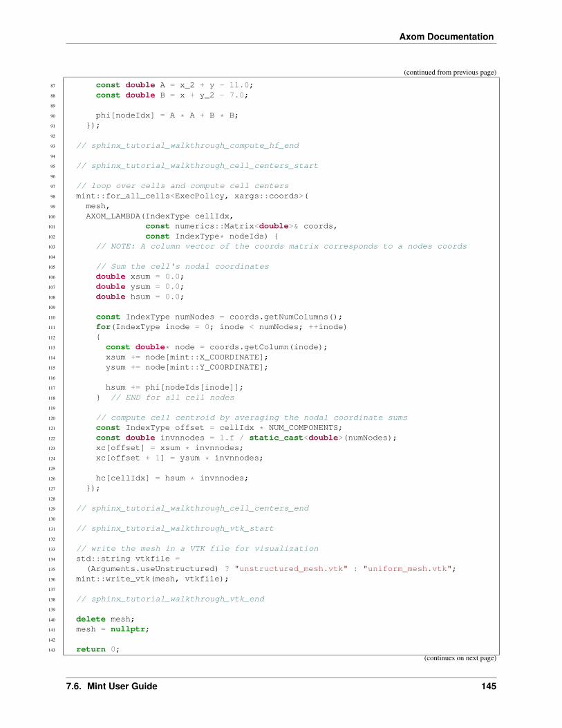
Axom Documentation


87 const double A = x_2 + y - 11.0;88 const double B = x + y_2 - 7.0;89

90 phi[nodeIdx] = A * A + B * B;91 );92

93 // sphinx_tutorial_walkthrough_compute_hf_end94

95 // sphinx_tutorial_walkthrough_cell_centers_start96

97 // loop over cells and compute cell centers98 mint::for_all_cells<ExecPolicy, xargs::coords>(99 mesh,

100 AXOM_LAMBDA(IndexType cellIdx,101 const numerics::Matrix<double>& coords,102 const IndexType* nodeIds) 103 // NOTE: A column vector of the coords matrix corresponds to a nodes coords104

105 // Sum the cell's nodal coordinates106 double xsum = 0.0;107 double ysum = 0.0;108 double hsum = 0.0;109

110 const IndexType numNodes = coords.getNumColumns();111 for(IndexType inode = 0; inode < numNodes; ++inode)112 113 const double* node = coords.getColumn(inode);114 xsum += node[mint::X_COORDINATE];115 ysum += node[mint::Y_COORDINATE];116

117 hsum += phi[nodeIds[inode]];118 // END for all cell nodes119

120 // compute cell centroid by averaging the nodal coordinate sums121 const IndexType offset = cellIdx * NUM_COMPONENTS;122 const double invnnodes = 1.f / static_cast<double>(numNodes);123 xc[offset] = xsum * invnnodes;124 xc[offset + 1] = ysum * invnnodes;125

126 hc[cellIdx] = hsum * invnnodes;127 );128

129 // sphinx_tutorial_walkthrough_cell_centers_end130

131 // sphinx_tutorial_walkthrough_vtk_start132

133 // write the mesh in a VTK file for visualization134 std::string vtkfile =135 (Arguments.useUnstructured) ? "unstructured_mesh.vtk" : "uniform_mesh.vtk";136 mint::write_vtk(mesh, vtkfile);137

138 // sphinx_tutorial_walkthrough_vtk_end139

140 delete mesh;141 mesh = nullptr;142

143 return 0;(continues on next page)


Axom Documentation


144 145

146 //------------------------------------------------------------------------------147 // FUNCTION PROTOTYPE IMPLEMENTATION148 //------------------------------------------------------------------------------149 void parse_args(int argc, char** argv)150 151 Arguments.res = 25;152 Arguments.useUnstructured = false;153

154 for(int i = 1; i < argc; ++i)155 156 if(strcmp(argv[i], "--unstructured") == 0)157 158 Arguments.useUnstructured = true;159 160

161 else if(strcmp(argv[i], "--resolution") == 0)162 163 Arguments.res = std::atoi(argv[++i]);164 165

166 // END for all arguments167

168 SLIC_ERROR_IF(169 Arguments.res < 2,170 "invalid mesh resolution! Please, pick a value greater than 2.");171 172

173 //------------------------------------------------------------------------------174 // sphinx_tutorial_walkthrough_construct_umesh_start175 mint::Mesh* getUniformMesh()176 177 // construct a N x N grid within a domain defined in [-5.0, 5.0]178 const double lo[] = -5.0, -5.0;179 const double hi[] = 5.0, 5.0;180 mint::Mesh* m = new mint::UniformMesh(lo, hi, Arguments.res, Arguments.res);181 return (m);182 183 // sphinx_tutorial_walkthrough_construct_umesh_end184

185 //------------------------------------------------------------------------------186 mint::Mesh* getUnstructuredMesh()187 188 mint::Mesh* umesh = getUniformMesh();189 const IndexType umesh_ncells = umesh->getNumberOfCells();190 const IndexType umesh_nnodes = umesh->getNumberOfNodes();191

192 const IndexType ncells = umesh_ncells * 4; // split each quad into 4 triangles193 const IndexType nnodes = umesh_nnodes + umesh_ncells;194

195 constexpr int DIMENSION = 2;196 using MeshType = mint::UnstructuredMesh<mint::SINGLE_SHAPE>;197 MeshType* m = new MeshType(DIMENSION, mint::TRIANGLE, nnodes, ncells);198 m->resize(nnodes, ncells);199

200 double* x = m->getCoordinateArray(mint::X_COORDINATE);(continues on next page)


Axom Documentation


201 double* y = m->getCoordinateArray(mint::Y_COORDINATE);202 IndexType* cells = m->getCellNodesArray();203

204 // fill coordinates from uniform mesh205 mint::for_all_nodes<ExecPolicy, xargs::xy>(206 umesh,207 AXOM_LAMBDA(IndexType nodeIdx, double nx, double ny) 208 x[nodeIdx] = nx;209 y[nodeIdx] = ny;210 );211

212 // loop over cells, compute cell centers and fill connectivity213 mint::for_all_cells<ExecPolicy, xargs::coords>(214 umesh,215 AXOM_LAMBDA(IndexType cellIdx,216 const numerics::Matrix<double>& coords,217 const IndexType* nodeIds) 218 // NOTE: A column vector of the coords matrix corresponds to a nodes coords219

220 // Sum the cell's nodal coordinates221 double xsum = 0.0;222 double ysum = 0.0;223 for(IndexType inode = 0; inode < NUM_NODES_PER_CELL; ++inode)224 225 const double* node = coords.getColumn(inode);226 xsum += node[mint::X_COORDINATE];227 ysum += node[mint::Y_COORDINATE];228 // END for all cell nodes229

230 // compute cell centroid by averaging the nodal coordinate sums231 const IndexType nc = umesh_nnodes + cellIdx; /* centroid index */232 x[nc] = xsum * ONE_OVER_4;233 y[nc] = ysum * ONE_OVER_4;234

235 // triangulate236 const IndexType& n0 = nodeIds[0];237 const IndexType& n1 = nodeIds[1];238 const IndexType& n2 = nodeIds[2];239 const IndexType& n3 = nodeIds[3];240

241 const IndexType offset = cellIdx * 12;242

243 cells[offset] = n0;244 cells[offset + 1] = nc;245 cells[offset + 2] = n3;246

247 cells[offset + 3] = n0;248 cells[offset + 4] = n1;249 cells[offset + 5] = nc;250

251 cells[offset + 6] = n1;252 cells[offset + 7] = n2;253 cells[offset + 8] = nc;254

255 cells[offset + 9] = n2;256 cells[offset + 10] = n3;257 cells[offset + 11] = nc;



Axom Documentation


258 );259

260 // delete uniform mesh261 delete umesh;262 umesh = nullptr;263

264 return (m);265

AXOM_LAMBDA Macro

The AXOM_LAMBDA convenience macro expands to:

• [=] capture by value when the Axom Toolkit is compiled without CUDA.

• [=] __host__ __device__ when the Axom Toolkit is compiled with CUDA

Raw Sidre Data

1 2 "name": "",3 "groups":4 5 "state":6 7 "name": "state",8 "groups":9

10 "t1":11 12 "name": "t1",13 "views":14 15 "block_id":16 17 "name": "block_id",18 "schema": "\"dtype\":\"int32\", \"number_of_elements\": 1, \"offset\":

→˓0, \"stride\": 4, \"element_bytes\": 4, \"endianness\": \"little\"",19 "value": "-1",20 "state": "SCALAR",21 "is_applied": 122 ,23 "partition_id":24 25 "name": "partition_id",26 "schema": "\"dtype\":\"int32\", \"number_of_elements\": 1, \"offset\":

→˓0, \"stride\": 4, \"element_bytes\": 4, \"endianness\": \"little\"",27 "value": "-1",28 "state": "SCALAR",29 "is_applied": 130 31 32 33



../../../../../index.html

../../../../../index.html

Axom Documentation


34 ,35 "coordsets":36 37 "name": "coordsets",38 "groups":39 40 "c1":41 42 "name": "c1",43 "views":44 45 "type":46 47 "name": "type",48 "schema": "\"dtype\":\"char8_str\", \"number_of_elements\": 9, \

→˓"offset\": 0, \"stride\": 1, \"element_bytes\": 1, \"endianness\": \"little\"",49 "value": "\"explicit\"",50 "state": "STRING",51 "is_applied": 152 53 ,54 "groups":55 56 "values":57 58 "name": "values",59 "views":60 61 "x":62 63 "name": "x",64 "schema": "\"dtype\":\"float64\", \"number_of_elements\": 6, \

→˓"offset\": 0, \"stride\": 8, \"element_bytes\": 8, \"endianness\": \"little\"",65 "value": "[0.0, 2.0, 1.0, 3.5, 2.5, 5.0]",66 "state": "BUFFER",67 "is_applied": 168 ,69 "y":70 71 "name": "y",72 "schema": "\"dtype\":\"float64\", \"number_of_elements\": 6, \

→˓"offset\": 0, \"stride\": 8, \"element_bytes\": 8, \"endianness\": \"little\"",73 "value": "[0.0, 0.0, 1.0, 1.0, 2.0, 0.0]",74 "state": "BUFFER",75 "is_applied": 176 77 78 79 80 81 82 ,83 "topologies":84 85 "name": "topologies",86 "groups":87



Axom Documentation


88 "t1":89 90 "name": "t1",91 "views":92 93 "coordset":94 95 "name": "coordset",96 "schema": "\"dtype\":\"char8_str\", \"number_of_elements\": 3, \

→˓"offset\": 0, \"stride\": 1, \"element_bytes\": 1, \"endianness\": \"little\"",97 "value": "\"c1\"",98 "state": "STRING",99 "is_applied": 1

100 ,101 "type":102 103 "name": "type",104 "schema": "\"dtype\":\"char8_str\", \"number_of_elements\": 13, \

→˓"offset\": 0, \"stride\": 1, \"element_bytes\": 1, \"endianness\": \"little\"",105 "value": "\"unstructured\"",106 "state": "STRING",107 "is_applied": 1108 109 ,110 "groups":111 112 "elements":113 114 "name": "elements",115 "views":116 117 "shape":118 119 "name": "shape",120 "schema": "\"dtype\":\"char8_str\", \"number_of_elements\": 4, \

→˓"offset\": 0, \"stride\": 1, \"element_bytes\": 1, \"endianness\": \"little\"",121 "value": "\"tri\"",122 "state": "STRING",123 "is_applied": 1124 ,125 "connectivity":126 127 "name": "connectivity",128 "schema": "\"dtype\":\"int32\", \"number_of_elements\": 12, \

→˓"offset\": 0, \"stride\": 4, \"element_bytes\": 4, \"endianness\": \"little\"",129 "value": "[1, 3, 2, 2, 0, 1, 3, 4, 2, 1, 5, 3]",130 "state": "BUFFER",131 "is_applied": 1132 ,133 "stride":134 135 "name": "stride",136 "schema": "\"dtype\":\"int32\", \"number_of_elements\": 1, \

→˓"offset\": 0, \"stride\": 4, \"element_bytes\": 4, \"endianness\": \"little\"",137 "value": "3",138 "state": "SCALAR",139 "is_applied": 1



Axom Documentation


140 141 142 143 144 145 146 ,147 "fields":148 149 "name": "fields",150 "groups":151 152 "den":153 154 "name": "den",155 "views":156 157 "association":158 159 "name": "association",160 "schema": "\"dtype\":\"char8_str\", \"number_of_elements\": 8, \

→˓"offset\": 0, \"stride\": 1, \"element_bytes\": 1, \"endianness\": \"little\"",161 "value": "\"element\"",162 "state": "STRING",163 "is_applied": 1164 ,165 "volume_dependent":166 167 "name": "volume_dependent",168 "schema": "\"dtype\":\"char8_str\", \"number_of_elements\": 5, \

→˓"offset\": 0, \"stride\": 1, \"element_bytes\": 1, \"endianness\": \"little\"",169 "value": "\"true\"",170 "state": "STRING",171 "is_applied": 1172 ,173 "topology":174 175 "name": "topology",176 "schema": "\"dtype\":\"char8_str\", \"number_of_elements\": 3, \

→˓"offset\": 0, \"stride\": 1, \"element_bytes\": 1, \"endianness\": \"little\"",177 "value": "\"t1\"",178 "state": "STRING",179 "is_applied": 1180 ,181 "values":182 183 "name": "values",184 "schema": "\"dtype\":\"float64\", \"number_of_elements\": 4, \"offset\

→˓": 0, \"stride\": 8, \"element_bytes\": 8, \"endianness\": \"little\"",185 "value": "[0.5, 1.2, 2.5, 0.9]",186 "state": "BUFFER",187 "is_applied": 1188 189 190 191 192



Axom Documentation


193 194

7.7 Primal User Guide

Primal is a component of Axom that provides efficient and general purpose algorithms and data structures for compu-tational geometry. Primal provides:

• Classes to represent geometric primitives such as Point and Ray

• Functions operating on Primal’s classes to implement geometric operators, including distance and intersection

This tutorial contains a collection of brief examples demonstrating Primal primitives and operators. The examplesinstantiate geometric primitives as needed and demonstrate geometric operators. These examples also show represen-tative overloads of each of the Primal operators (see the API documentation for more details).



Primitives

Primal includes the following primitives:

• Point

• Segment, Ray, Vector

• Plane, Triangle, Polygon

• Sphere

• Tetrahedron

• BoundingBox, OrientedBoundingBox

Primal also provides the NumericArray class, which implements arithmetic operations on numerical tuples and sup-ports Primal’s Point and Vector classes. Classes in Primal are templated on coordinate type (double, float, etc.) anddimension. The primitives do not inherit from a common base class. This was a design choice in favor of simplicityand performance. Geometric primitives can be tested for equality and can be printed to strings.

Primal also includes functions to merge a pair of BoundingBox or a pair of OrientedBoundingBox objects and to createnew OrientedBoundingBox objects from a list of points.

The following includes header files for primal’s primitives as well as some using directives and typedef state-ments that will be used in the examples. Header files for operations will be shown next to code examples. Althoughthe examples #include separate class header files, it is easier and less error-prone to write #include axom/primal.hpp.

// Axom primitives#include "axom/primal/geometry/BoundingBox.hpp"#include "axom/primal/geometry/OrientedBoundingBox.hpp"#include "axom/primal/geometry/Point.hpp"#include "axom/primal/geometry/Polygon.hpp"#include "axom/primal/geometry/Ray.hpp"



../../../../doxygen/html/primaltop.html

../../../../doxygen/html/primaltop.html

Axom Documentation


#include "axom/primal/geometry/Segment.hpp"#include "axom/primal/geometry/Triangle.hpp"#include "axom/primal/geometry/Vector.hpp"

// "using" directives to simplify codenamespace primal = axom::primal;

// almost all our examples are in 3Dconstexpr int in3D = 3;

// primitives represented by doubles in 3Dusing PointType = primal::Point<double, in3D>;using TriangleType = primal::Triangle<double, in3D>;using BoundingBoxType = primal::BoundingBox<double, in3D>;using OrientedBoundingBoxType = primal::OrientedBoundingBox<double, in3D>;using PolygonType = primal::Polygon<double, in3D>;using RayType = primal::Ray<double, in3D>;using SegmentType = primal::Segment<double, in3D>;using VectorType = primal::Vector<double, in3D>;

Operators

Primal implements geometric operators with unbound functions. Currently, these include the following:

• clip finds the polygon resulting from a bounding box clipping a triangle.

• closest_point takes a primitive P and a query point Q and returns the point on P closest to Q.

• compute_bounding_box finds the bounding box for a given primitive.

• squared_distance computes the squared distance from a point to another primitive.

• orientation finds the side of a line segment or triangle where a query point lies.

• intersect predicate tests if two primitives intersect. Some of the combinations also indicate the point ofintersection of a 1D primitive with another primitive.

Note: Most use cases have low dimension, usually 2 or 3. Dimensionality has been generalized to support othervalues where it does not interfere with the common case, but some operators such as triangle intersection do notsupport other dimensionality than 2 or 3.

Note: Many of the operations includes a tolerance parameter eps for improved geometric robustness. For example,orientation() considers a point to be on the boundary (OrientationResult::ON_BOUNDARY) when thepoint is within eps of the plane. This parameter is explicitly exposed in the primal API for some operations (e.g.some versions of intersect()), but not others (e.g. orientation()).

Clip triangle against bounding box

The clip operator clips a triangle against a bounding box, returning the resulting polygon. The figure shows the trianglein blue and the polygon resulting from clip() in grey.

7.7. Primal User Guide 153

Axom Documentation

#include "axom/primal/operators/clip.hpp"

TriangleType tri(PointType 1.2, 0, 0,PointType 0, 1.8, 0,PointType 0, 0, 1.4);

BoundingBoxType bbox(PointType 0, -0.5, 0, PointType 1, 1, 1);

PolygonType poly = clip(tri, bbox);

Closest point query

The closest point operator finds the point on a triangle that is closest to a query point. Query point 𝑜 (shown in darkblue), at the origin, is closest to point 𝑜′ (light blue), which lies in the triangle’s interior. Query point 𝑎 (olive) is closestto point 𝑎′ (yellow), which lies on the triangle’s edge at a vertex.

#include "axom/primal/operators/closest_point.hpp"

TriangleType tri(PointType 1, 0, 0, PointType 0, 1, 0, PointType 0, 0, 1);

PointType pto = PointType 0, 0, 0;PointType pta = PointType -1, 2, 1;

// Query point o lies at the origin. Its closest point lies in the// interior of tri.PointType cpto = closest_point(pto, tri);

// Query point a lies farther from the triangle. Its closest point// is on tri's edge.int lcpta = 0;PointType cpta = closest_point(pta, tri, &lcpta);


Axom Documentation

As the code example shows, closest_point() can take a pointer to an int as an optional third parameter. Ifsupplied, the function writes a value into the int that indicates which of the triangle’s vertices or sides contains theclosest point (or the interior).

Compute bounding box

Primal’s bounding boxes are rectangular right prisms. That is, they are boxes where neighboring walls are at rightangles.

The BoundingBox class represents an axis-aligned bounding box, which has two walls perpendicular to the X-axis,two perpendicular to the Y-axis, and two perpendicular to the Z-axis. This is sufficient for many computations; rangeand intersection operations tend to be fast.

The OrientedBoundingBox class can be oriented in any way with respect to the coordinate axes. This can provide atighter fit to the bounded data, but construction, intersection, and range calculation are more costly.

Here a group of points is used to create both an (axis-aligned) BoundingBox and an OrientedBoundingBox. The pointsare drawn in blue, the BoundingBox in black, and the OrientedBoundingBox in orange.

#include "axom/primal/operators/compute_bounding_box.hpp"

// An array of Points to include in the bounding boxesconst int nbr_points = 6;PointType data[nbr_points] = PointType 0.6, 1.2, 1.0,

PointType 1.3, 1.6, 1.8,PointType 2.9, 2.4, 2.3,PointType 3.2, 3.5, 3.0,PointType 3.6, 3.2, 4.0,PointType 4.3, 4.3, 4.5;

// A BoundingBox constructor takes an array of Point objectsBoundingBoxType bbox(data, nbr_points);// Make an OrientedBoundingBoxOrientedBoundingBoxType obbox = compute_oriented_bounding_box(data, nbr_points);

Primal also provides a merge_boxes() function to produce a bounding box that contains two input bounding boxes.This is available for client codes to use and also supports the operation of the BVHTree class.


Axom Documentation

Intersection

The intersection test is provided by intersect(). It takes two primitives and returns a boolean indicating ifthe primitives intersect. Some overloads return the point of intersection in an output argument. The overloads forintersect() are summarized in the table below.

Arg 1 Arg 2 Additional arguments and notesTriangle Triangle include boundaries1 (default false)Ray Segment return intersection point. 2D only.Segment BoundingBox return intersection pointRay BoundingBox return intersection pointBoundingBox BoundingBoxSphere Sphere specify toleranceTriangle BoundingBoxTriangle Ray return parameterized intersection point (on Ray), return barycentric inter-

section point (on Triangle)Triangle Segment return parameterized intersection point (on Segment), return barycentric in-

tersection point (on Triangle)OrientedBound-ingBox

OrientedBound-ingBox

specify tolerance

The example below tests for intersection between two triangles, a ray, and a BoundingBox.

#include "axom/primal/operators/intersect.hpp"

// Two trianglesTriangleType tri1(PointType 1.2, 0, 0,

PointType 0, 1.8, 0,PointType 0, 0, 1.4);

TriangleType tri2(PointType 0, 0, 0.5,PointType 0.8, 0.1, 1.2,PointType 0.8, 1.4, 1.2);

// tri1 and tri2 should intersectif(intersect(tri1, tri2))std::cout << "Triangles intersect as expected." << std::endl;

else


1 By default, the triangle intersection algorithm considers only the triangles’ interiors, so that non-coplanar triangles that share two vertices arenot reported as intersecting. The caller to intersect() can specify an optional argument to include triangle boundaries in the intersection test.


Axom Documentation


std::cout << "There's an error somewhere..." << std::endl;

// A vertical ray constructed from origin and pointRayType ray(SegmentType(PointType 0.4, 0.4, 0, PointType 0.4, 0.4, 1));

// t will hold the intersection point between ray and tri1,// as parameterized along ray.double rt1t = 0;// rt1b will hold the intersection point barycentric coordinates,// and rt1p will hold the physical coordinates.PointType rt1b, rt1p;

// The ray should intersect tri1 and tri2.if(intersect(tri1, ray, rt1t, rt1b) && intersect(tri2, ray))// Retrieve the physical coordinates from barycentric coordinatesrt1p = tri1.baryToPhysical(rt1b);// Retrieve the physical coordinates from ray parameterPointType rt1p2 = ray.at(rt1t);std::cout << "Ray intersects tri1 as expected. Parameter t: " << rt1t

<< std::endl<< " Intersection point along ray: " << rt1p2 << std::endl<< " Intersect barycentric coordinates: " << rt1b << std::endl<< " Intersect physical coordinates: " << rt1p << std::endl<< "Ray also intersects tri2 as expected." << std::endl;

elsestd::cout << "There's an error somewhere..." << std::endl;

// A bounding boxBoundingBoxType bbox(PointType 0.1, -0.23, 0.1, PointType 0.8, 0.5, 0.4);

// The bounding box should intersect tri1 and ray but not tr2.PointType bbtr1;if(intersect(ray, bbox, bbtr1) && intersect(tri1, bbox) &&

!intersect(tri2, bbox))std::cout << "As hoped, bounding box intersects tri1 at " << bbtr1

<< " and ray, but not tri2." << std::endl;elsestd::cout << "There is at least one error somewhere..." << std::endl;

In the diagram, the point where the ray enters the bounding box is shown as the intersection point (not the exit pointor some point inside the box). This is because if a ray intersects a bounding box at more than one point, the firstintersection point along the ray (the intersection closest to the ray’s origin) is reported as the intersection. If a rayoriginates inside a bounding box, the ray’s origin will be reported as the point of intersection.


Axom Documentation

Orientation

Axom contains two overloads of orientation(). The 3D case tests a point against a triangle and reports whichside it lies on; the 2D case tests a point against a line segment. Here is an example of the 3D point-triangle orientationtest.

#include "axom/primal/operators/orientation.hpp"

// A triangleTriangleType tri(PointType 1.2, 0, 0,

PointType 0, 1.8, 0,PointType 0, 0, 1.4);

// Three points:// one on the triangle's positive side,PointType pos = PointType 0.45, 1.5, 1;// one coplanar to the triangle, the centroid,PointType cpl =PointType::lerp(PointType::lerp(tri[0], tri[1], 0.5), tri[2], 1. / 3.);

// and one on the negative sidePointType neg = PointType 0, 0, 0.7;

// Test orientationif(orientation(pos, tri) == primal::ON_POSITIVE_SIDE &&

orientation(cpl, tri) == primal::ON_BOUNDARY &&orientation(neg, tri) == primal::ON_NEGATIVE_SIDE)

std::cout << "As expected, point pos is on the positive side," << std::endl

<< " point cpl is on the boundary (on the triangle),"<< std::endl<< " and point neg is on the negative side." << std::endl;

elsestd::cout << "Someone wrote this wrong." << std::endl;

The triangle is shown with its normal vector pointing out of its centroid. The triangle’s plane divides space into apositive half-space, pointed into by the triangle’s normal vector, and the opposing negative half-space. The test pointon the 𝑧 axis, labelled 𝑁 , is on the negative side of the triangle. The centroid lies in the triangle, on the boundarybetween the two half-spaces. The remaining test point, labelled 𝑃 , is on the triangle’s positive side.


Axom Documentation

Distance

The various overloads of squared_distance() calculate the squared distance between a query point and severaldifferent primitives:

• another point,

• a BoundingBox,

• a Segment,

• a Triangle.

#include "axom/primal/operators/squared_distance.hpp"

// The point from which we'll queryPointType q = PointType::make_point(0.75, 1.2, 0.4);

// Find distance to:PointType p 0.2, 1.4, 1.1;SegmentType seg(PointType 1.1, 0.0, 0.2, PointType 1.1, 0.5, 0.2);TriangleType tri(PointType 0.2, -0.3, 0.4,

PointType 0.25, -0.1, 0.3,PointType 0.3, -0.3, 0.35);

BoundingBoxType bbox(PointType -0.3, -0.2, 0.7, PointType 0.4, 0.3, 0.9);

double dp = squared_distance(q, p);double dseg = squared_distance(q, seg);double dtri = squared_distance(q, tri);double dbox = squared_distance(q, bbox);

The example shows the squared distance between the query point, shown in black in the figure, and four geometricprimitives. For clarity, the diagram also shows the projection of the query point and its closest points to the XY plane.

7.8 Quest User Guide

The Quest component of Axom provides several spatial operations and queries on a mint::Mesh.

• Operations

– Read a surface mesh from an STL file

7.8. Quest User Guide 159

Axom Documentation

– Check for some common mesh errors; deduplicate vertices

* vertex welding: merge vertices closer than a specified distance “epsilon”

* find self-intersections and degenerate triangles in a surface mesh

* watertightness test: is a surface mesh a watertight manifold?

• Point queries

– Surface mesh point queries in C or in C++

* in/out query: is a point inside or outside a surface mesh?

* signed distance query: find the minimum distance from a query point to a surface mesh

– Point in cell query: for a query point, find the cell of the mesh that holds the point and the point’s isopara-metric coordinates within that cell

– All nearest neighbors: given a list of point locations and regions, find all neighbors of each point in adifferent region



Reading in a mesh

Applications commonly need to read a mesh file from disk. Quest provides the STLReader class, which can readbinary or ASCII STL files, as well as the PSTLReader class for use in parallel codes. STL (stereolithography) isa common file format for triangle surface meshes. The STL reader classes will read the file from disk and build amint::Mesh object.

The code examples are excerpts from the file <axom>/src/tools/mesh_tester.cpp.

We include the STL reader header

#include "axom/quest/readers/STLReader.hpp"

and also the mint Mesh and UnstructuredMesh headers.

#include "axom/mint/mesh/Mesh.hpp"#include "axom/mint/mesh/UnstructuredMesh.hpp"

For convenience, we use typedefs in the axom namespace.

using namespace axom;

using UMesh = mint::UnstructuredMesh<mint::SINGLE_SHAPE>;

The following example shows usage of the STLReader class:

// Read fileSLIC_INFO("Reading file: '" << params.stlInput << "'...\n");quest::STLReader* reader = new quest::STLReader();reader->setFileName(params.stlInput);reader->read();

// Get surface mesh



../../../../doxygen/html/questtop.html

https://en.wikipedia.org/wiki/STL_(file_format)

Axom Documentation


UMesh* surface_mesh = new UMesh(3, mint::TRIANGLE);reader->getMesh(surface_mesh);

// Delete the readerdelete reader;reader = nullptr;

SLIC_INFO("Mesh has " << surface_mesh->getNumberOfNodes() << " vertices and "<< surface_mesh->getNumberOfCells() << " triangles.");

After reading the STL file, the STLReader::getMesh method gives access to the underlying mesh data. Thereader may then be deleted.

Check and repair a mesh

The STL file format specifies triangles without de-duplicating their vertices. Vertex welding is needed for several meshalgorithms that require a watertight manifold. Additionally, mesh files often contain errors and require some kind ofcleanup. The following code examples are excerpts from the file <axom>/src/tools/mesh_tester.cpp.

Quest provides a function to weld vertices within a distance of some specified epsilon. This func-tion takes arguments mint::UnstructuredMesh< mint::SINGLE_SHAPE > **surface_mesh anddouble epsilon, and modifies surface_mesh. In addition to the mint Mesh and UnstructuredMesh headers(see previous page), we include the headers declaring the functions for checking and repairing surface meshes.

#include "axom/quest/MeshTester.hpp"

The function call itself:

quest::weldTriMeshVertices(&surface_mesh, params.weldThreshold);

One problem that can occur in a surface mesh is self-intersection. A well-formed mesh will have each triangle touchingthe edge of each of its neighbors. Intersecting or degenerate triangles can cause problems for some spatial algorithms.To detect such problems using Quest, we first make containers to record defects that might be found.

std::vector<std::pair<int, int>> collisions;std::vector<int> degenerate;

Then, we call the function to detect self-intersections and degenerate triangles.

// Use a uniform grid spatial indexquest::findTriMeshIntersections(surface_mesh,

collisions,degenerate,params.resolution,params.intersectionThreshold);

After calling findTriMeshIntersections, collisions will hold the indexes of each pair of intersectingtriangles and degenerate will contain the index of each degenerate triangle. The user code can then address orreport any triangles found. Mesh repair beyond welding close vertices is beyond the scope of the Quest component.

Check for watertightness

Before using Quest’s surface point queries, a mesh must be watertight, with no cracks or holes. Quest provides afunction to test for watertightness, declared in the same header file as the tests self-intersection and an enum indicating


Axom Documentation

watertightness of a mesh. If the code is working with a mesh read in from an STL file, weld the vertices (see above)before checking for watertightness!

quest::WatertightStatus wtstat = quest::isSurfaceMeshWatertight(surface_mesh);

This routine builds the face relation of the supplied triangle surface mesh. The face of a triangle is a one-dimensionaledge. If the mesh is big, building the face relation may take some time. Once built, the routine queries face relation:each edge of every triangle must be incident in two triangles. If the mesh has a defect where more than two trianglesshare an edge, the routine returns CHECK_FAILED. If the mesh has a hole, at least one triangle edge is incident inonly one triangle and the routine returns NOT_WATERTIGHT. Otherwise, each edge is incident in two triangles, andthe routine returns WATERTIGHT.

After testing for watertightness, report the result.

switch(wtstat)case quest::WatertightStatus::WATERTIGHT:

std::cout << "The mesh is watertight." << std::endl;break;

case quest::WatertightStatus::NOT_WATERTIGHT:std::cout << "The mesh is not watertight: at least one "

<< "boundary edge was detected." << std::endl;break;

default:std::cout << "An error was encountered while checking." << std::endl

<< "This may be due to a non-manifold mesh." << std::endl;break;

After an STL mesh has

• been read in with STLReader,

• had vertices welded using weldTriMeshVertices(),

• contains no self-intersections as reported by findTriMeshIntersections(),

• and is watertight as reported by isSurfaceMeshWatertight(),

the in-out and distance field queries will work as designed.

Surface mesh point queries: C API

Quest provides the in/out and distance field queries to test a point against a surface mesh. These queries take a meshcomposed of triangles in 3D and a query point. The in/out query tests whether the point is contained within the surfacemesh. The distance query calculates the signed distance from the query point to the mesh.

The following examples show Quest’s C interface to these queries. The general pattern is to set some query parameters,then pass a mint::Mesh * or file name string to an initialization function, call an evaluate function for eachquery point, then clean up with a finalize function.

In/out C API

The in/out query operates on a 3D surface mesh, that is, triangles forming a watertight surface enclosing a 3D vol-ume. The in/out API utilizes integer-valued return codes with values quest::QUEST_INOUT_SUCCESS andquest::QUEST_INOUT_FAILED to indicate the success of each operation. These examples are excerpted from<axom>/src/axom/quest/examples/quest_inout_interface.cpp.


Axom Documentation

Fig. 7.27: Types of point-vs-surface-mesh queries provided by Quest. Left: In/out query, characterizing points asinside or outside the mesh. Points that lie on the boundary might or might not be categorized as inside the mesh.Right: Distance query, calculating the signed distance from each query point to its closest point on the mesh. Anegative result indicates an interior query point.

To get started, we first include some header files.

#include "axom/quest/interface/inout.hpp"

#ifdef AXOM_USE_MPI#include <mpi.h>

#endif

Before initializing the query, we can set some parameters, for example, to control the logging verbosity and to set athreshold for welding vertices of the triangle mesh while generating the spatial index.

// -- Set quest_inout parametersrc = quest::inout_set_verbose(isVerbose);if(rc != quest::QUEST_INOUT_SUCCESS)cleanAbort();

// Note: contour files are only supported when Axom is configured with C2Cusing axom::utilities::string::endsWith;const int dim = endsWith(fileName, ".contour") ? 2 : 3;rc = quest::inout_set_dimension(dim);if(rc != quest::QUEST_INOUT_SUCCESS)cleanAbort();

rc = quest::inout_set_vertex_weld_threshold(weldThresh);if(rc != quest::QUEST_INOUT_SUCCESS)cleanAbort();

rc = quest::inout_set_segments_per_knot_span(segmentsPerKnotSpan);if(rc != quest::QUEST_INOUT_SUCCESS)cleanAbort();

By default, the verbosity is set to false and the welding threshold is set to 1E-9.


Axom Documentation

We are now ready to initialize the query.

#ifdef AXOM_USE_MPIrc = quest::inout_init(fileName, MPI_COMM_WORLD);

#elserc = quest::inout_init(fileName);

#endif

The variable fileName is a std::string that indicates a triangle mesh file. Another overload ofquest::inout_init() lets a user code pass a reference to a mint::Mesh* to query meshes that were pre-viously read in or built up. If initialization succeeded (returned quest::QUEST_INOUT_SUCCESS), the code can

• Query the mesh bounds with quest::inout_mesh_min_bounds(double[3]) andquest::inout_mesh_max_bounds(double[3]).

• Find mesh center of mass with quest::inout_mesh_center_of_mass(double[3]).

• Test if a query point is inside the mesh surface. In this example pt is a double[3] and numInside is arunning total.

const bool ins = quest::inout_evaluate(pt[0], pt[1], pt[2]);numInside += ins ? 1 : 0;

Once we are done, we clean up with the following command:

quest::inout_finalize();

Signed Distance query C API

Excerpted from <axom>/src/axom/quest/examples/quest_signed_distance_interface.cpp.

Quest header:

#include "axom/quest.hpp"

Before initialization, a code can set some parameters for the distance query.

• Passing true to quest::signed_distance_set_closed_surface(bool) lets the user read in anon-closed “terrain mesh” that divides its bounding box into “above” (positive distance to the surface mesh) and“below” (negative distance).

• quest::signed_distance_set_execution_space() allows setting the execution space to run thesigned distance query in. The following values are accepted:

– quest::SignedDistExec::CPU runs the signed distance query on the CPU.

– quest::SignedDistExec::OpenMP runs the signed distance query with multiple threads on theCPU using OpenMP. Requires building Axom with OpenMP support.

– quest::SignedDistExec::GPU runs the signed distance query on the GPU, if supported. Thiscurrently requires CUDA support.

• quest::signed_distance_set_allocator() allows setting a custom Umpire allocator to allocatethe underlying BVH in. The allocator should be compatible with the execution space set in the call toquest::signed_distance_set_execution_space().

• If the SLIC logging environment is in use, passing true to quest::signed_distance_set_verbose()will turn on verbose logging.


Axom Documentation

• Use of MPI-3 shared memory can be enabled by passing true toquest::signed_distance_use_shared_memory().

The distance query must be initialized before use. In this example, Arguments is a POD struct containing parametersto the executable. As with the in/out query, a user code may pass either a file name or a reference to a mint::Mesh* to quest::signed_distance_init().

int rc = quest::signed_distance_init(args.fileName, global_comm);

Once the query is initialized, the user code may retrieve mesh bounds withquest::signed_distance_get_mesh_bounds(double* lo, double* hi). Test query pointsagainst the mesh with quest::signed_distance_evaluate(). Here, pt is a double[3], phi is adouble array, and inode is an integer.

phi[inode] = quest::signed_distance_evaluate(pt[0], pt[1], pt[2]);

Finally, clean up.

quest::signed_distance_finalize();

Surface mesh point queries: C++ API

Codes written in C++ may use the object-oriented C++ APIs to perform in/out and signed distance queries. In additionto language choice, the C++ API lets a code work with more than one mesh at the same time. Unlike the C API, theC++ API for in/out and signed distance queries has no initializer taking a file name: readying the mesh is a separate,prior step.

In/out Octree

The C++ in/out query is provided by the quest::InOutOctree class, from the following header. See <axom>/src/axom/quest/tests/quest_inout_octree.cpp.

#include "axom/quest/InOutOctree.hpp"

Some type aliases are useful for the sake of brevity. The class is templated on the dimensionality of the mesh. Cur-rently, only meshes in 3D are supported; here DIM equals 3.

using Octree3D = axom::quest::InOutOctree<DIM>;

using GeometricBoundingBox = Octree3D::GeometricBoundingBox;using SpacePt = Octree3D::SpacePt;

Instantiate the object using GeometricBoundingBox bbox and a mesh, and generate the index.

Octree3D octree(bbox, mesh);octree.generateIndex();

Test a query point.

SpacePt pt = SpacePt::make_point(2., 3., 1.);bool inside = octree.within(pt);

All cleanup happens when the index object’s destructor is called (in this case, when the variable octree goes out ofscope).


Axom Documentation

Signed Distance

The C++ signed distance query is provided by the quest::SignedDistance class, which wraps an instanceof primal::BVHTree. Examples from <axom>/src/axom/quest/tests/quest_signed_distance.cpp.

Class header:

#include "axom/primal/geometry/Point.hpp"

#include "axom/quest/SignedDistance.hpp" // quest::SignedDistance

The constructor takes several arguments:

• const mint::Mesh* surfaceMesh: A pointer to a surface mesh with triangles and/or quadrilaterals.

• bool isWatertight: Indicates the mesh is a watertight mesh, a manifold. The signed distance from a pointto a manifold is mathematically well-defined. When the input is not a closed surface mesh, the mesh must spanthe entire computational mesh domain, dividing it into two regions.

• bool computeSign (default true): Optional. Enables or disables the computation of signs in distancequeries.

• int allocatorID: Optional. Sets a custom Umpire allocator to use in constructing the underlying BVH;by default, this is set to a default allocator for the execution space the SignedDistance class is instantiatedin (host-side memory for CPU and OpenMP, unified memory for GPUs).

Note that the second and subsequent arguments to the constructor correspond toquest::signed_distance_set functions in the C API.

As with the InOutOctree, the class is templated on the dimensionality of the mesh, with only 3D meshes beingsupported. The class also accepts a template parameter for execution space, for running signed distance queries withOpenMP or on a GPU.

// Set execution spaceconstexpr int BlockSize = 256;using ExecSpace = axom::CUDA_EXEC<BlockSize>;

// Create a custom allocatorconstexpr size_t PoolSize = 1024 * 1024 * 1024;umpire::ResourceManager& rm = umpire::ResourceManager::getInstance();umpire::Allocator device_allocator =rm.makeAllocator<umpire::strategy::QuickPool>(

"DEVICE_POOL",rm.getAllocator(umpire::resource::Device),PoolSize);

int device_pool_id = device_allocator.getId();

// Set SignedDistance optionsconstexpr bool is_watertight = true;constexpr bool compute_signs = true;quest::SignedDistance<3, ExecSpace> signed_distance(surface_mesh,

is_watertight,compute_signs,device_pool_id);

Test a query point.


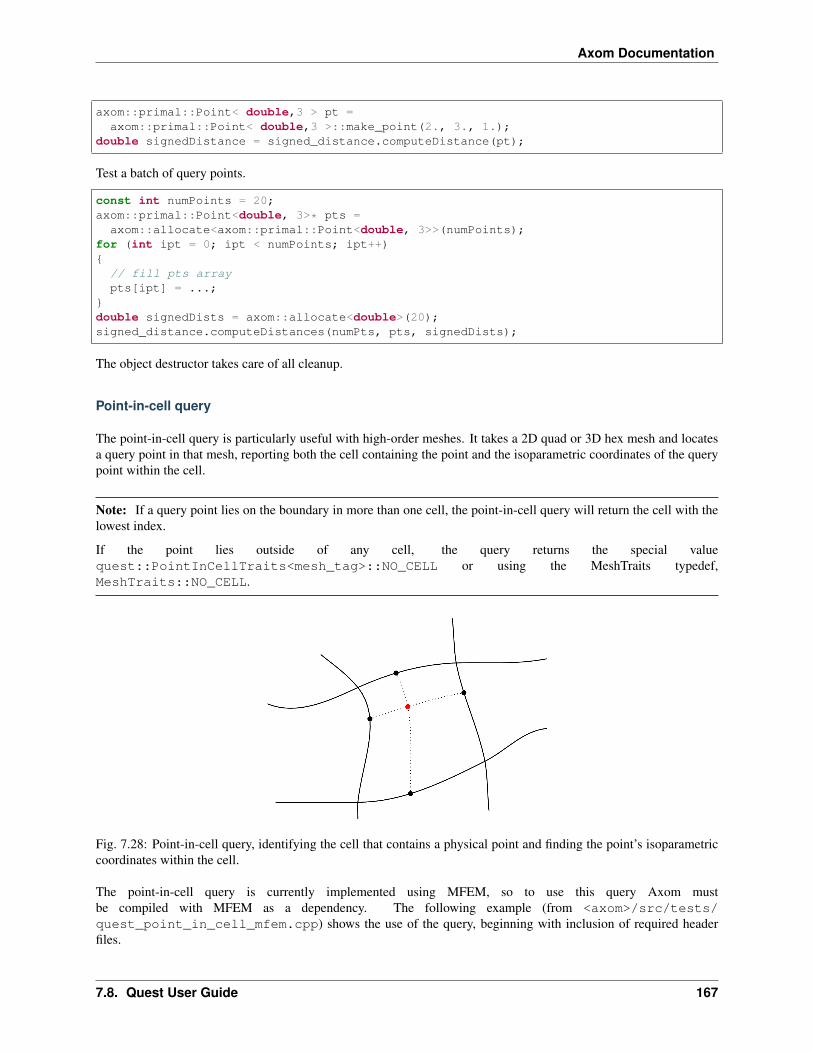
Axom Documentation

axom::primal::Point< double,3 > pt =axom::primal::Point< double,3 >::make_point(2., 3., 1.);

double signedDistance = signed_distance.computeDistance(pt);

Test a batch of query points.

const int numPoints = 20;axom::primal::Point<double, 3>* pts =

axom::allocate<axom::primal::Point<double, 3>>(numPoints);for (int ipt = 0; ipt < numPoints; ipt++)

// fill pts arraypts[ipt] = ...;

double signedDists = axom::allocate<double>(20);signed_distance.computeDistances(numPts, pts, signedDists);

The object destructor takes care of all cleanup.

Point-in-cell query

The point-in-cell query is particularly useful with high-order meshes. It takes a 2D quad or 3D hex mesh and locatesa query point in that mesh, reporting both the cell containing the point and the isoparametric coordinates of the querypoint within the cell.

Note: If a query point lies on the boundary in more than one cell, the point-in-cell query will return the cell with thelowest index.

If the point lies outside of any cell, the query returns the special valuequest::PointInCellTraits<mesh_tag>::NO_CELL or using the MeshTraits typedef,MeshTraits::NO_CELL.

Fig. 7.28: Point-in-cell query, identifying the cell that contains a physical point and finding the point’s isoparametriccoordinates within the cell.

The point-in-cell query is currently implemented using MFEM, so to use this query Axom mustbe compiled with MFEM as a dependency. The following example (from <axom>/src/tests/quest_point_in_cell_mfem.cpp) shows the use of the query, beginning with inclusion of required headerfiles.


Axom Documentation

#include "axom/quest/PointInCell.hpp"

#ifdef AXOM_USE_MFEM#include "axom/quest/detail/PointInCellMeshWrapper_mfem.hpp"

#else#error "Quest's PointInCell tests on mfem meshes requires mfem library."

#endif

We use typedefs for the sake of brevity. The class is templated on a struct (provided by Quest, referred to asmesh_tag) that is used to select MFEM as the backend implementation for point location. To implement a newbackend, a developer must declare a new (empty) struct and provide a specialization of the PointInCellTraitsand PointInCellMeshWrapper templated on the new struct that fulfill the interface documented for those classes.

using mesh_tag = axom::quest::quest_point_in_cell_mfem_tag;using PointInCellType = axom::quest::PointInCell<mesh_tag, ExecSpace>;using MeshTraits = typename PointInCellType::MeshTraits;using IndexType = typename PointInCellType::IndexType;

Instantiate the object using an MFEM mesh and a spatial index 25 bins on a side.

PointInCellType spatialIndex(m_mesh, GridCell(25).data(), m_EPS, m_allocatorID);

Test a query point. Here idx receives the ID of the cell that contains queryPoint and isoPar is aprimal::Point that receives the isoparametric coordinates of queryPoint within cell idx.

spatialIndex.locatePoints(pts, outCellIds.data(), outIsopar.data());

From cell ID and isoparametric coordinates, reconstruct the input physical coordinates.

SpacePt untransformPt;spatialIndex.reconstructPoint(idx, isoPar.data(), untransformPt.data());

The destructor of the index object cleans up resources used (in this case, when the variable spatialIndex goes outof scope).

All nearest neighbors query

Some applications need to work with the interaction of points that are close to each other. For example, in onetechnique used for additive manufacturing, the particles in a powder bed are melted using a laser. Particle behavioragainst nearby particles determines droplet formation. The all-nearest-neighbors query takes as input a list of pointpositions and regions and a maximum radius. For each point, using the L2 norm as the distance measure, the querycalculates the nearest neighbor point not in the same region, as shown in the figure.

Here is an example of query usage, from <axom>/src/axom/quest/tests/quest_all_nearest_neighbors.cpp.

First, include the header.

#include "axom/quest/AllNearestNeighbors.hpp"

Query input consists of the points’ x, y, and z positions and region IDs, the point count, and the search radius.

double x[] = -1.2, -1.0, -0.8, -1.0, 0.8, 1.0, 1.2, 1.0;double y[] = 0.0, -0.2, 0.0, 0.2, 0.0, -0.2, 0.0, 0.2;double z[] = 0.0, 0.0, 0.0, 0.0, 0.0, 0.0, 0.0, 0.0;int region[] = 0, 0, 0, 0, 1, 1, 1, 1;



Axom Documentation

Fig. 7.29: All nearest neighbors query. Here, points belong to one of four regions. Given a maximum search radius,the query finds the closest neighbor to each point in another region.


int n = 8;double limit = 1.9;

For each input point, the output arrays give the point’s neighbor index and squared distance from the point to thatneighbor.

axom::quest::all_nearest_neighbors(x, y, z, region, n, limit, neighbor, dsq);

7.9 Sidre User Guide

The Sidre (Simulation data repository) component of Axom provides tools to centralize data management in HPCapplications: data description, allocation, access, and so forth. The goal of Sidre is efficient coordination and sharingof data across physics packages in integrated applications, and between applications and tools that provide capabilitiessuch as file I/O, in situ visualization, and analysis.

The design of Sidre is based on substantial production application experience and requirements for codes to run onadvanced architectures. Such codes must carefully manage data allocation and placement to run efficiently. Sidre isintended to be used in a variety of diverse applications.



7.9.2 Introduction

Sidre provides simple application-level semantics to describe, allocate, deallocate, and provide access to data. Cur-rently supported capabilities include:

7.9. Sidre User Guide 169

../../../../doxygen/html/sidretop.html

Axom Documentation

• Separate data description and allocation operations. This allows applications to describe their data and thendecide how best to place the data in memory.

• Multiple different “views” into a chunk of (shared) data. A Sidre view includes description semantics todefine data type, number of elements, offset, stride, etc. Thus, a chunk of data in memory can be interpretedconceptually in different ways using different views into it.

• Externally-owned “opaque” or described data. Sidre can accept a pointer to externally-allocated data andprovide access to it by name. When external data is described to Sidre, it can be processed in the same ways asdata that Sidre owns. When data is not described (i.e., it is “opaque”), Sidre can provide access to the data via apointer, but the consumer of the data must know type information to do anything substantial with the data.

• Support for different memory spaces and allocation schemes. Default memory space and allocation supportis basic. More advanced features are available via the Umpire library when Axom is configured to be built withit.

• Attributes or metadata associated with a Sidre view. This metadata is available to user code to facilitateprogram logic and is also used in Axom to enable selective writing of data subsets to files.

• Tree-structured data hierarchies. Many mesh-based application codes organize data into hierarchies of con-texts (e.g., domains, regions, blocks, mesh centerings, subsets of elements containing different materials, etc.).Sidre supports hierarchical, tree-based organizations in a simple, flexible way that aligns with the data organi-zation in many applications.

• APIs for C++, C, and Fortran along with mechanisms to ensure inter-language data consistency.

So far, Sidre development has focused on designing and building flexible and powerful concepts to build on. The SidreAPI includes five main concepts:

• DataStore. The main access point to data managed by Sidre; it contains a collection of Buffers, a collection ofdefault Attributes, and a tree structure of Groups.

• Buffer. Describes and holds a chunk of data in memory owned by Sidre.

• Group. Defines a tree structure like a filesystem, where Groups are like folders and Views are like files.

• View. Describes a conceptual layout of data in memory. Each View has a collection of its explicitly-set At-tributes.

• Attribute. Provides a metadata descriptor of a View.

These concepts will be described in more detail in later sections.

At this point, Sidre supports simple data types such as scalars, strings, and (multidimensional) arrays of scalars.Fundamentally, Sidre does not preclude the use of more complex data structures, but does not currently support themdirectly. Future Sidre development will expand core functionality to support additional features such as:

• Support for more complex data types.

• Complex queries and actions involving Attributes.

Support for these enhancements and others will be added based on application needs and use cases.

An introductory example

As an introduction to the core concepts in Sidre and how they work, here is an example where we construct the Sidredata hierarchy structure shown in the following figure:

The diagram represents a datastore container, holding all Sidre objects and provides the main interface to access thoseobjects. Rounded rectangles represent Sidre Group objects. Each Group has a name and one parent group, exceptfor the root group (i.e. “/”), which has no parent. A datastore provides one root group (i.e. “/”) that is created whena DataStore object is constructed; thus, an application does not create the root. A Group may have zero or more


https://github.com/LLNL/Umpire

Axom Documentation

Symbol Sidre class

Group

View

Attribute


Axom Documentation

child groups (indicated by an arrow from the parent to each child). Each group also owns zero or more View objects,which are shown as rectangles. An arrow points from a group to each view it owns.

A Sidre View object has a name and, typically, some data associated with it. This example shows various types ofdata that can be described by a view, including scalars, strings, and data in arrays (both externally allocated and ownedby Sidre Buffer objects). Each array view has a data pointer and describes data in terms of data type, number ofelements, offset, and stride. Data pointers held by array view are shown as dashed arrows.

A DataStore also contains a collection of Buffer objects, shown as segmented rectangles.

A DataStore contains a list of Attribute objects. Each Attribute is outlined with a hexagon and definesa metadata label and a default value associated with that label. In the example, the datastore has “vis” (with defaultvalue 0) and “restart” (with default value 1) attributes. Default attributes apply to all views unless explicitly set forindividual views. In the example, the “temp” and “rho” views have the “vis” attribute set to 1.

Various aspects of Sidre usage are illustrated in the C++ code shown next. Sidre provides full C and Fortran APIs thatcan also be used to generate the same result.

First, we create a DataStore object, define some Attribute objects along with their default values, and add somechild Group objects to the root Group.

// Create Sidre datastore object and get root groupDataStore* ds = new DataStore();Group* root = ds->getRoot();

// Create two attributesds->createAttributeScalar("vis", 0);ds->createAttributeScalar("restart", 1);

// Create group children of root groupGroup* state = root->createGroup("state");Group* nodes = root->createGroup("nodes");Group* fields = root->createGroup("fields");

The createViewScalar() method lets an application store scalar values in a view owned by the group object themethod is called on.

// Populate "state" groupstate->createViewScalar("cycle", 25);state->createViewScalar("time", 1.2562e-2);state->createViewString("name", "sample_20171206_a");

This example stores (x, y, z) node position data in one array. The array is managed by a Buffer object and threeView objects point into it. C++ Sidre operations that create a Buffer, a Group, and a View, as shown in thefollowing code, return a pointer to the object that is created. This allows chaining operations. (Chaining is supportedin the C++ API but not in C or Fortran.)

int N = 16;int nodecount = N * N * N;int eltcount = (N - 1) * (N - 1) * (N - 1);

// Populate "nodes" group//// "x", "y", and "z" are three views into a shared Sidre buffer object that// holds 3 * nodecount doubles. These views might describe the location of// each node in a 16 x 16 x 16 hexahedron mesh. Each view is described by// number of elements, offset, and stride into that data.Buffer* buff = ds->createBuffer(sidre::DOUBLE_ID, 3 * nodecount)->allocate();nodes->createView("x", buff)->apply(sidre::DOUBLE_ID, nodecount, 0, 3);



Axom Documentation


nodes->createView("y", buff)->apply(sidre::DOUBLE_ID, nodecount, 1, 3);nodes->createView("z", buff)->apply(sidre::DOUBLE_ID, nodecount, 2, 3);

The last two integral arguments to the createView() method specify the offset from the beginning of the array andthe stride of the data. Thus, the x, y, z values for each position are stored contiguously with the x values, y values, andz values each offset from each other by a stride of three in the array.

The next snippet creates two views (“temp” and “rho”) and allocates each of their data as an array of type double withlength ‘eltcount’. Then, it sets an attribute (“vis”) on each view with a value of 1. Lastly, it creates a group (“ext”)that has a view holding an external pointer (“region”). The apply() method describes the view data as an array ofinteger type and length ‘eltcount’. Note that it is the responsibility of the caller to ensure that the allocation to whichthe “region” pointer references is adequate to contain that data description.

// Populate "fields" group//// "temp" is a view into a buffer that is not shared with another View.// In this case, the data Buffer is allocated directly through the View// object. Likewise with "rho." Both Views have the default offset (0)// and stride (1). These Views could point to data associated with// each of the 15 x 15 x 15 hexahedron elements defined by the nodes above.View* temp = fields->createViewAndAllocate("temp", sidre::DOUBLE_ID, eltcount);View* rho = fields->createViewAndAllocate("rho", sidre::DOUBLE_ID, eltcount);

// Explicitly set values for the "vis" Attribute on the "temp" and "rho"// buffers.temp->setAttributeScalar("vis", 1);rho->setAttributeScalar("vis", 1);

// The "fields" Group also contains a child Group "ext" which holds a pointer// to an externally owned integer array. Although Sidre does not own the// data, the data can still be described to Sidre.Group* ext = fields->createGroup("ext");// int * region has been passed in as a function argument. As with "temp"// and "rho", view "region" has default offset and stride.ext->createView("region", region)->apply(sidre::INT_ID, eltcount);

The next code example shows various methods to retrieve a group object and data from a view in the group hierarchy.

// Retrieve Group pointersGroup* root = ds->getRoot();Group* state = root->getGroup("state");Group* nodes = root->getGroup("nodes");Group* fields = root->getGroup("fields");

// Accessing a Group that is not there gives a null pointer// Requesting a nonexistent View also gives a null pointerGroup* goofy = root->getGroup("goofy");if(goofy == nullptr)std::cout << "no such group: goofy" << std::endl;

elsestd::cout << "Something is very wrong!" << std::endl;



Axom Documentation


// Access items in "state" groupint cycle = state->getView("cycle")->getScalar();double time = state->getView("time")->getScalar();const char* name = state->getView("name")->getString();

// Access some items in "nodes" and "fields" groupsdouble* y = nodes->getView("y")->getArray();int ystride = nodes->getView("y")->getStride();double* temp = fields->getView("temp")->getArray();int* region = fields->getView("ext/region")->getArray();

// Nudge the 3rd node, adjust temp and region of the 3rd elementy[2 * ystride] += 0.0032;temp[2] *= 1.0021;region[2] = 6;

In the last section, the code accesses the arrays associated with the views “y”, “temp”, and “region”. While “temp”and “region” have the default offset (0) and stride (1), “y” has offset 1 and stride 3 (as described earlier). The pointerreturned by View::getPointer() always points to the first data element described by the view (the view takescare of the offset), but use of a stride other than 1 must be done by the code itself.

Unix-style path syntax using the slash (“/”) delimiter is supported for traversing Sidre group and view hierarchies andaccessing their contents. However, ‘..’ and ‘.’ syntax (up-directory and current directory) is not supported. This usageis shown in the last call to getView() in the code example above. The method call retrieves the view named “region”in the group named “ext” that is a child of the “fields” group. Character sequences before the first slash and betweentwo consecutive slashes are assumed to be group names (describing parent-child relationships). For this method, andothers dealing with view objects, the sequence following the last slash is assumed to be the name of a view. Similarpath syntax can be used to retrieve a group, create a group and a view, a nd so forth.

Core concepts

As noted earlier and described in the previous example, Sidre provides five main classes: DataStore, Buffer,Group, View, and Attribute. In combination, these classes implement a data store with a tree structure toorganize data in a hierarchy. Before delving into details of these classes/concepts, we summarize their basic intent:

• DataStore is the main interface to access a data hierarchy.

• Buffer describes and holds a contiguous chunk of data in memory.

• Group defines parent-child relationships in a hierarchical tree data structure and provides access to file I/Ooperations.

• View provides a virtual description of data and access to it.

• Attribute allows a program to attach metadata to View objects for processing data selectively.

The following sections summarize the main interface features and functionality of these Sidre classes.

Note: Interfaces for each of these classes are provided natively in C++, C, and Fortran.

DataStore

A Sidre DataStore object provides the main access point for Sidre contents, including the data managed by Sidre.A datastore maintains the Group object at the root of a Sidre data hierarchy, a collection of Buffer objects, and


Axom Documentation

a collection of Attribute objects. Generally, the first thing a Sidre user does is create the datastore object; thisoperation also creates the root group. Apart from providing access to the root group, a datastore provides methods toretrieve and interact with buffers and attributes.

Note: Buffer and Attribute objects can only be created and destroyed using DataStore methods notedbelow. The Buffer and Attribute class constructors and destructors are private.

The DataStore class provides the following methods to manage and interact with Buffer objects:

• Create, destroy, and allocate data in buffers

• Query the number of buffers that exist

• Query whether a buffer exists with a given id

• Retrieve the buffer with a given id

• Iterate over the set of buffers in a datastore

Please see Buffer for more information about using Buffer objects.

The DataStore class provides the following methods to manage and interact with Attribute objects:

• Create and destroy attributes

• Query the number of attributes that exist

• Query whether an attribute exists with a given name or id

• Retrieve attribute with a given name or id

• Iterate over the set of attributes in a datastore

Please see Attribute for more information about using Attribute objects.

Buffer

A Sidre Buffer object holds a contiguous array of data described by a data type and length. The data owned by abuffer is unique to that buffer; i.e., buffers do not share data.

A buffer can be created without a data description and then described later in a separate operation, or it can be describedwhen it is created. In either case, data description and allocation are distinct operations. This allows an applicationto create buffers it needs, then assess the types and amount of data they will hold before deciding how and when toallocate data.

Note:

• Buffer objects can only be created and destroyed using DataStore class methods. Buffer constructor anddestructor methods are private (see DataStore).

• Each Buffer object has a unique integer identifier generated when the buffer is created. If you want to retrievea buffer or interact with it directly, you must keep a pointer to it or note its id so that you can retrieve it from aDataStore when needed.

Buffer objects hold data for Sidre View objects in most cases. Each buffer maintains references to the views thatrefer to its data. These references are created when a buffer object is attached to a view, or when data is allocated witha view. Data stored in a buffer may be accessed through a view or through the buffer. See View for more informationabout View objects.


Axom Documentation

The Buffer class provides the following operations:

• Retrieve the unique id of the buffer

• Query whether a buffer is described or allocated

• Describe buffer data (type and number of elements)

• Allocate, reallocate, deallocate buffer data

• Copy a given number of bytes of data from a given pointer to a buffer allocation

• Get data held by a buffer as a pointer or conduit::Node::Value type

• Query the data owned by a buffer: type, number of elements, total number of bytes, number of bytes per element,etc.

• Retrieve the number of views the buffer is attached to

• Copy buffer description and its data to/from a conduit::Node

Group

Sidre Group objects are used to define a tree-like hierarchical organization for application data, such as meshes andfields used in a simulation. Each group has a name and one parent group (except for the root group, which has noparent) and contains zero or more child groups and zero or more data views. A Sidre datastore has exactly one rootgroup that is created when the datastore is created. The root group’s name is initially the empty string. See DataStorefor more information.

A group hierarchy is constructed by creating child groups of the root group, children of those groups, and so on. Allgroups in a subtree rooted at a particular group are considered descendants of that group. View objects can be createdin groups to hold or provide access to data of various types.

Note: Group and View objects can only be created and destroyed using Group class methods. The Group andView class constructors and destructors are private.

A group or view is owned by the group that created it; i.e., its parent group or owning group, respectively. Groups andviews maintain pointers to their parent/owning group. Thus, one may walk up or down a group hierarchy to accessgroups and views in it, as needed.

Note:

• The name (string) of a group or view must be unique within its parent/owning Group.

• A group or view has a unique integer identifier within its parent/owning group, which is generated when it iscreated.

• Views and child groups in a group can be accessed by name or integer id.

A group can be moved or copied to another group. When a group is moved to another group, it is removed from itsoriginal parent and the group to which it is moved becomes its parent. This implies that the entire subtree of groupsand views within the moved group is moved as well and can no longer be accessed via the original parent group. Whena group is copied to another group, a copy of the entire group subtree rooted at the copied group is added to the groupto which it is copied. A shallow copy is performed for the data in each view. Specifically, a new view objects iscreated in the destination, but the data is shared by the original and new view.


Axom Documentation

Note: View object copy operations perform shallow copies of the data in a view.

Some methods for creating, destroying, querying, and retrieving groups and views take a string with path syntax,where parent and child group names are joined with the path separator character ‘/’. Other methods take the name ofan immediate child of a group. Methods that require the name of an immediate child are marked with ‘Child’ in theirname, such as hasChildView() and hasChildGroup(). When a path string is passed to a method that acceptspath syntax, the last item in the path indicates the item to be created, destroyed, accessed, etc. For example,:

View* view = group->createView("foo/bar/baz");

is equivalent to:

View* view = group->createGroup("foo")->createGroup("bar")->createView("baz");

In particular, intermediate groups “foo” and “bar” will be created in this case if they don’t already exist. The pathsyntax is similar to a Unix filesystem, but the path string may not contain the parent entry, such as “../foo”, or currentgroup, such as “./bar”.

Methods to Operate on Groups

The following lists summarize Group class methods that support operations related to groups.

Note:

• Methods that access groups by index only work with the immediate children of the current group because an idhas no meaning outside of the indexing of the current group. None of these methods is marked with ‘Child’ inits name.

• When a group is created, destroyed, copied, or moved, ids of other views and groups in its parent group maybecome invalid. This is analogous to iterator invalidation for containers when the container contents change.

Create, Modify, and Destroy Groups

• Create a child group given a name (child) or path (other descendant). If a path is given, intermediate groups inpath are created, if needed.

• Rename a group. A group cannot be renamed to the empty string, to a string containing the path separatorcharacter, or to the name of another group or view owned by the same parent.

• Destroy a descendant group with given id (child), or name/path (child or other descendant).

• Destroy all child groups in a group.

Note: When a Group object is destroyed, all groups and views in the subtree rooted at the destroyed group are alsodestroyed. However, the data associated with the views will remain intact.

Group Properties

• Retrieve the name or id of a group


Axom Documentation

• Retrieve the full path name from the root of the tree to a group

• Get a pointer to the parent group of a group

• Query the number of child groups of a group

• Query whether a group has a descendant group with a given name or path

• Query whether a group has an immediate child group with a given integer id

• Query the name of a child group with a given id, or the id of a child group with a given name

• Get a pointer to the datastore that owns the hierarchy in which a group resides

Group Access

• Retrieve an immediate child group with a given name or id, or a descendant group with a given path

• Iterate over the set of child groups of a group

Move and Copy Groups

• Move a group, and its associated subtree, from its parent group and make it a child of another group

• Create a copy of group subtree rooted at some group and make it a child of another group

• Query whether a group subtree is equivalent to another; i.e., identical subtree structures with same names for allgroups and views, and views are also equivalent (see View Property Operations).

Methods to Operate on Views

Group class methods that support operations related to View objects are summarized below. For more details onView concepts and operations, please see View.

Note: Methods that access views by index work only with the views owned by the current group because an id hasno meaning outside of the indexing of the current group. None of these methods is marked with ‘Child’ in its name.

Create Views

• Create a view in the group with a name only.

• Create a view in the group with a name and data description.

• Create a view in the group with a name and with a Buffer attached. The View may or may not have a datadescription.

• Create a view in the group with a name and an external data pointer. The data may or may not be described.

• Create a view in the group with a name and data description, and allocate the data. Implicitly the data is held ina buffer that is attached to the view.

• Create a view in the group with a name holding a given scalar or string.


Axom Documentation

Destroy Views

• Destroy view with given id (child), or name/path (view in the group or some descendant group), and leave viewdata intact.

• Destroy all views in the group, and leave their data intact.

• Destroy view with given id, or name/path, and destroy their data.

• Destroy all views in the group and destroy their data.

View Queries

• Query the number of views in a group.

• Query whether a group subtree has a view with a given name or path.

• Query whether a group has a view with a given integer id.

• Query the name of a view with a given id, or the id of a view with a given name.

View Access

• Retrieve a view in the group with a given name or id, or a descendant view (somewhere in the subtree) with agiven path.

• Iterate over the set of views owned by the group.

Move and Copy Views

• Move a view from its owning group to another group (removed from original owning group).

• Copy a view to another group. Note that this is a shallow copy of the view data; i.e., it is shared by the originaland the new view in the destination group.

Group I/O Operations

The group interface provides methods to perform data I/O operations on views in the group subtree rooted at anygroup.

• Copy a description of a group subtree to a conduit::Node.

• Create native and external data layouts in conduit::Node hierarchies (used mainly for I/O operations)

• Save and load group subtrees, including data in associated views, to and from files. A variety of methods areprovided to support different I/O operations, different I/O protocols, etc.

I/O methods on the group class use Conduit to write the data (sub)tree rooted in a group to a file, HDF5 handle, orother Conduit protocol, or to an in-memory Conduit data structure. Please see Sidre Interaction with Conduit for moreinformation. An application may provide an attribute to the method call, so only views with that attribute explicitlyset will be written. See Parallel File I/O for more information.



https://www.hdfgroup.org/HDF5/

Axom Documentation

View

A Sidre View object describes data and provides access to it. A view can describe a (portion of a) data allocation inany way that is compatible with the allocation. Specifically, the allocation must contain enough bytes to support thedescription. In particular, the data type of a view description need not match the types associated with the allocationor types of other views that refer to that data.

Note: View objects can only be created and destroyed using Group class methods. The View class constructor anddestructor are private.

Each view has a name and is owned by one group in a Sidre group hierarchy; i.e., its owning group. A view maintainsa pointer to the group that owns it.

Note:

• The name (string) of a view must be unique within its owning group.

• A view has a unique integer identifier within its owning group, which is generated when the view is created.

• Views in a group can be accessed by name or integer id.

A view can describe and provide access to data referenced by a pointer in one of four ways described below. A viewdata description includes: data type, length (number of elements), offset (from base data pointer) and stride (based onthe pointer address and data type).

• A view can describe (a subset of) data owned by a pre-existing buffer. In this case, the buffer is manuallyattached to the view and the view’s data description is applied to the buffer data. Buffer data can be (re)allocatedor deallocated by the view if and only if it is the only view attached to the buffer. In general, a buffer can beattached to more than one view.

• A view description can be used to allocate data for the view using a View class allocate() method similarto buffer data description and allocation (see Buffer). In this case, the view is usually exclusively associatedwith a buffer and no other view is allowed to (re)allocate or deallocate the data held by the buffer.

• A view can describe data associated with a pointer to an external data allocation. In this case, the view cannot(re)allocate or deallocate the data. However, all other view operations can be applied to the data in essentiallythe same ways as the previous two cases.

• A view can hold a pointer to an undescribed (opaque) data pointer. In this case, the view knows nothing aboutthe type or structure of the data; it can only provide access to it. A user is entirely responsible for casting thepointer to a proper type when accessed through the view, knowing the size of the data, etc.

A view may also refer to a scalar quantity or a string. Such views hold their data differently than the pointer casesdescribed above.

Before we describe the Sidre View class interface, we present some view concepts that describe various states a viewcan be in at any given time. Hopefully, this will provide some useful context for the method descriptions that follow.

The key view concepts that users should be aware of are:

• View data description (data type, number of elements, stride, offset, etc.)

• View data association (data lives in an attached Sidre buffer, accessed via an external pointer, or is a scalar orstring owned by the view)

• Whether the view data description has been applied to the data

The table below summarizes View data associations (rows) and view states with respect to the data (columns).


Axom Documentation

Fig. 7.30: This table summarizes Sidre view data associations and data states. Each row is a data association and eachcolumn refers to a data state. The True/False entries in the cells indicate return values of the View class methods atthe tops of the columns. The circumstances under which those values are returned are noted as well.


Axom Documentation

The three View data state methods at the tops of columns and their return values are:

• isDescribed() returns true if a view has a data description, and false otherwise.

• isAllocated() returns true if a view is associated with data, such as a non-null pointer, and false otherwise.

• isApplied() returns true if a view has a data description and is associated with data that is compatible with thatdescription, and the description has been applied to the data; otherwise false is returned.

The rows indicate data associations; the View class has methods to query these as well; e.g., isEmpty(),hasBuffer(), etc. The associations are:

• EMPTY. A view has no associated data; the view may or may not have a data description.

• BUFFER. A view has an attached buffer; the view may or may not have a data description and the buffer mayor may not be allocated and the description (if view has one) may or may not be applied to the buffer data (ifallocated).

• EXTERNAL. A view has a non-null pointer to external data; the view may or may not have a data descriptionand the description, if the view has one, may or may not be applied to the external data.

• SCALAR. A view was created to hold a scalar value; such a view always has a valid data description, isallocated, and the description is applied.

• STRING. A view was created to hold a string; such a view always has a valid data description, is allocated, andthe description is applied.

Note that there are specific consequences that follow from each particular association/state that a view is in. Forexample, an EMPTY view cannot have an attached buffer. Neither can an EXTERNAL, SCALAR or STRING view.A view that is EMPTY, BUFFER, SCALAR, or STRING cannot be EXTERNAL, etc.

The following lists summarize the View class interface:

Note: Most View class methods return a pointer to the view object on which the method is called. This allowsoperations to be chained; e.g.,

View* view = ...;view->describe(...)->allocate(...)->apply();

View Property Operations

• Retrieve the name or id of the view object.

• Retrieve the view path name from the root of the tree or the path to the group that owns it.

• Get a pointer to the group that owns the view.

• Is the view equivalent to another view; i.e., are names and data descriptions the same?

• Rename a view.

• Clear the view by removing description and data.

Data Association Queries

• Is view empty?

• Does view have a buffer attached?


Axom Documentation

• Is view associated with external data?

• Is it a scalar view?

• Is it a string view?

Data State Queries

• Does view have a data description?

• Is view data allocated?

• Is view data description applied to data?

• Is view opaque; i.e., it has an external pointer and no description?

Data Description Queries

• Get the type of the data described by a view.

• Get total number of bytes of data.

• Get number of elements (total bytes / size of type).

• Get number of bytes per data element (for type).

• Get data offet.

• Get data stride.

• Get number of dimensions and shape of multi-dimensional data.

• Get a conduit::Schema object that contains the view data description.

Data Management Operations

• Allocate, reallocate, and deallocate view data.

• Attach buffer to view (with or without data description), and detach buffer from view.

• Apply current view description to data or apply a new description.

• Set view scalar value.

• Set view string.

• Set external data pointer, with or without a data description.

Data Access Methods

• Get a pointer to the view data, actual type or void*.

• Get scalar value for a scalar view.

• Retrieve pointer to buffer attached to view.

• Get a conduit::Node object that holds the view data.


Axom Documentation

Attribute Methods

• Query whether a view has an attribute with given id or name.

• Get attribute associated with a view by id or name.

• Query whether aAttribute has been set explicitly for view.

• Reset attribute with given id or name to its default value.

• Set attribute with given id or name to a given scalar value or string.

• Retrieve scalar value or string of an attribute.

• Iterate over attributes of a view.

I/O Operations

• Copy view data description to a conduit::Node.

Attribute

Sidre Attribute objects enable users to attach metadata (strings and values) to Sidre views to support queries(e.g., search for views with a given attribute name), outputting data for a subset of views to files, and other ways anapplication may need to selectively process views in a Sidre data hierarchy.

An attribute is created with a string name and a default scalar or string value. A default value can be changed later asneeded.

Note:

• Attribute objects can only be created and destroyed using DataStore class methods. The Attributeclass constructor and destructor are private (see DataStore).

• Each Attribute object has a unique name and integer identifier. Either can be used to retrieve anAttribute object from a DataStore object..

Each Sidre view inherits all attributes contained in a datastore with their default strings or values. Then, an applicationmay explicitly set any attribute on a view. The application may also query the value of a view attribute, query whetherthe attribute was explicitly set, or set the attribute back to its default value. See View for more information about Viewobjects.

The Attribute class provides the following operations:

• Retrieve the name and unique id of an attribute

• Set the scalar or string value of an attribute

• Get the type of an attribute’s scalar value

Data vs. Metadata Concepts

This section includes examples that illustrate some common Sidre usage patterns involving buffers, groups, and views.In particular, it shows how data associated with a view is related to a buffer, how the lifetimes of a view, its associateddata, and the buffer owning the data are related, and how the description of data in a view (metadata) is independentof the the allocation state of the data in a view and a corresponding buffer.


Axom Documentation

Note: Object and data creation and destruction is very explicit in Sidre to allow maximum flexibility to composecomplex operations from simpler ones. This should become apparent by following the examples.

The code snippets shown and described here exist in the file axom/src/axom/sidre/examples/sidre_data_vs_metadata.cpp, which can be built and run to experiment with if you wish.

The starting point for the first three examples is a simple Sidre datastore group hierarchy in which the root group hastwo child groups named “A” and “B”. The generation of this structure is shown in the following code along with someprint statements to verify the state is what we expect.

DataStore* ds = new DataStore();Group* root_grp = ds->getRoot();

Group* A_grp = root_grp->createGroup("A");Group* B_grp = root_grp->createGroup("B");

//// Initially, datastore contains no buffer objects since no data has// been allocated yet. Also, the groups have no views.//std::cout << "Datastore start state...." << std::endl;std::cout << "\tNum buffers in datastore: " << ds->getNumBuffers() << std::endl;std::cout << "\tNum views in group A: " << A_grp->getNumViews() << std::endl;std::cout << "\tNum views in group B: " << B_grp->getNumViews() << std::endl;

As expected, the datastore has no buffers and the groups have no views, which we can see from the output of the code:

Datastore start state....Num buffers in datastore: 0Num views in group A: 0Num views in group B: 0

Example 1: One View, One Buffer

The first example shows a common Sidre usage pattern in which a view is created in a group and the data associatedwith the view is managed via the view. This case represents a one-to-one relationship between a view and a buffer.

We begin by creating a view named “aview” in group “A” describing an integer array of length 10 and allocate it, allin one method call. This creates a buffer in the datastore which holds the array data. Then, we get a pointer to the startof the array from the view and initialize the array values. To give some insight into how Sidre works, we access andprint various pieces of information about the state of the group, view, and buffer. We also print the value of the bufferarray at slot 5 to confirm that the buffer is indeed holding the view’s data. Here’s the relevant code section.

const int dat_size = 10;

View* aview = A_grp->createViewAndAllocate("aview", INT_ID, dat_size);std::cout << "After A_grp->createViewAndAllocate() call\n";std::cout << "\tNum views in group A: " << A_grp->getNumViews() << std::endl;axom::IndexType nelems = aview->getNumElements();std::cout << "\tNum elements in view: " << nelems << std::endl;

Buffer* buf1 = aview->getBuffer();std::cout << "\tNum buffers in datastore: " << ds->getNumBuffers() << std::endl;std::cout << "\tNum views attached to buffer: " << buf1->getNumViews()



Axom Documentation


<< std::endl;std::cout << "\tNum elements in buffer array: " << buf1->getNumElements()

<< std::endl;

int* a_array = aview->getArray();for(axom::IndexType i = 0; i < nelems; ++i)a_array[i] = i + 2;


std::cout << "After initialization of view array\n";int* buf1_ptr = buf1->getData();std::cout << "\tValue of elt 5 in buffer array (expect 7): " << buf1_ptr[5]

<< std::endl;

The output printed by the code is:

After A_grp->createViewAndAllocate() callNum views in group A: 1Num elements in view: 10Num buffers in datastore: 1Num views attached to buffer: 1Num elements in buffer array: 10

After initialization of view arrayValue of elt 5 in buffer array (expect 7): 7

Next, we deallocate the view and show that its description remains intact; for example, the number of elements is still10. The view is still attached to the buffer. The view is no longer allocated since the buffer data was deallocated. Thebuffer’s data description remains intact.

Then, we allocate the view again. Since the buffer is still attached to the view, a new buffer is not created in thedatastore and the existing buffer is re-allocated. The same data description as before is used for the allocation sincewe haven’t changed it. We verify this in the code output which follows the code snippet (i.e., the datastore still hasone buffer).

aview->deallocate();std::cout << "After view deallocate call, the data no longer exists,\n"

<< "but the view description remains." << std::endl;std::cout << "\tNum elements in view: " << aview->getNumElements() << std::endl;std::cout << "\tView has buffer? " << aview->hasBuffer() << std::endl;std::cout << "\tIs view allocated? " << aview->isAllocated() << std::endl;std::cout << "\tNum buffers in datastore: " << ds->getNumBuffers() << std::endl;std::cout << "\tIs buffer allocated? " << buf1->isAllocated() << std::endl;std::cout << "\tNum views attached to buffer: " << buf1->getNumViews()

<< std::endl;std::cout << "\tNum elements in buffer array: " << buf1->getNumElements()

<< std::endl;


aview->allocate();std::cout << "After allocating view again...\n";std::cout << "\tNum buffers in datastore: " << ds->getNumBuffers() << std::endl;



Axom Documentation


std::cout << "\tIs buffer allocated? " << buf1->isAllocated() << std::endl;std::cout << "\tIs view allocated? " << aview->isAllocated() << std::endl;std::cout << "\tNum elements in view: " << aview->getNumElements() << std::endl;

The output of the code is:

After view deallocate call, the data no longer exists,but the view description remains.

Num elements in view: 10View has buffer? 1Is view allocated? 0Num buffers in datastore: 1Is buffer allocated? 0Num views attached to buffer: 1Num elements in buffer array: 10

After allocating view again...Num buffers in datastore: 1Is buffer allocated? 1Is view allocated? 1Num elements in view: 10

Lastly, we destroy the view and its data with a single method call and verify that the view and associated buffer nolonger exist.

A_grp->destroyViewAndData("aview");std::cout << "After destroyViewAndData() call\n";std::cout << "\tNum views in group A: " << A_grp->getNumViews() << std::endl;std::cout << "\tNum buffers in datastore: " << ds->getNumBuffers() << std::endl;

The output of this portion of code is:

After destroyViewAndData() callNum views in group A: 0Num buffers in datastore: 0

Example 2: Two Views, One Buffer

The second example illustrates a Sidre usage pattern in which multiple views are created to describe distinct portionsof data held in a shared buffer. This case represents a many-to-one relationship between views and a buffer. Beforewe start, we verify that the datastore contains no buffers and that the groups we created earlier contain no views.

We start by creating and allocating a buffer holding an array of doubles of length 10. We initialize the array so thateach element has a value matching its position in the array; i.e., the values 0 through 9. Then, we create two viewsin group “A” and attach each to the buffer. Next, we apply a data description containing an offset and stride to eachview so that one view is associated with the even values in the buffer and the other is associated with the odd values.Accessing the data pointer in each view and printing the values shows that this is indeed the case.

We call a method to destroy the first view and its data, similar to the last part of the first example. The view isdestroyed. However, since the buffer that held its data is shared by the other view, the buffer and its data remain intact.In particular, the data associated with the remaining view is also untouched.

std::cout << "\nDatastore start state\n";std::cout << "\tNum buffers in datastore: " << ds->getNumBuffers() << std::endl;std::cout << "\tNum views in group A: " << A_grp->getNumViews() << std::endl;



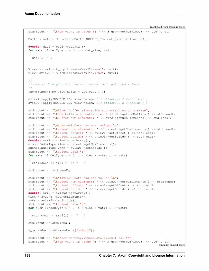
Axom Documentation


std::cout << "\tNum views in group B: " << B_grp->getNumViews() << std::endl;

Buffer* buf2 = ds->createBuffer(DOUBLE_ID, dat_size)->allocate();

double* dat2 = buf2->getData();for(axom::IndexType i = 0; i < dat_size; ++i)dat2[i] = i;

View* aview1 = A_grp->createView("aview1", buf2);View* aview2 = A_grp->createView("aview2", buf2);

//// aview1 data gets even values, aview2 data gets odd values.//axom::IndexType view_nelem = dat_size / 2;

aview1->apply(DOUBLE_ID, view_nelem, 0 /*offset*/, 2 /*stride*/);aview2->apply(DOUBLE_ID, view_nelem, 1 /*offset*/, 2 /*stride*/);

std::cout << "\nAfter buffer allocation and attaching to views\n";std::cout << "\tNum buffers in datastore: " << ds->getNumBuffers() << std::endl;std::cout << "\tBuffer num elements: " << buf2->getNumElements() << std::endl;

std::cout << "\n\taview1 data has even values:\n";std::cout << "\taview1 num elements: " << aview1->getNumElements() << std::endl;std::cout << "\taview1 offset: " << aview1->getOffset() << std::endl;std::cout << "\taview1 stride: " << aview1->getStride() << std::endl;double* arr1 = aview1->getArray();axom::IndexType vlen = aview1->getNumElements();axom::IndexType vstr = aview1->getStride();std::cout << "\taview1 data:\t";for(axom::IndexType i = 0; i < vlen * vstr; i += vstr)

std::cout << arr1[i] << " ";std::cout << std::endl;

std::cout << "\n\taview2 data has odd values:\n";std::cout << "\taview2 num elements: " << aview2->getNumElements() << std::endl;std::cout << "\taview2 offset: " << aview2->getOffset() << std::endl;std::cout << "\taview2 stride: " << aview2->getStride() << std::endl;double* arr2 = aview2->getArray();vlen = aview2->getNumElements();vstr = aview2->getStride();std::cout << "\taview2 data:\t";for(axom::IndexType i = 0; i < vlen * vstr; i += vstr)

std::cout << arr2[i] << " ";std::cout << std::endl;

A_grp->destroyViewAndData("aview1");

std::cout << "\nAfter destroyViewAndData(aview1) call\n";std::cout << "\tNum views in group A: " << A_grp->getNumViews() << std::endl;



Axom Documentation


std::cout << "\tNum buffers in datastore: " << ds->getNumBuffers() << std::endl;std::cout << "\tBuffer num elements: " << buf2->getNumElements() << std::endl;std::cout << "\taview2 data still has its odd values:\t";arr2 = aview2->getArray();vlen = aview2->getNumElements();vstr = aview2->getStride();for(axom::IndexType i = 0; i < vlen * vstr; i += vstr)std::cout << arr2[i] << " ";


Datastore start stateNum buffers in datastore: 0Num views in group A: 0Num views in group B: 0

After buffer allocation and attaching to viewsNum buffers in datastore: 1Buffer num elements: 10

aview1 data has even values:aview1 num elements: 5aview1 offset: 0aview1 stride: 2aview1 data: 0 2 4 6 8

aview2 data has odd values:aview2 num elements: 5aview2 offset: 1aview2 stride: 2aview2 data: 1 3 5 7 9

After destroyViewAndData(aview1) callNum views in group A: 1Num buffers in datastore: 1Buffer num elements: 10aview2 data still has its odd values: 1 3 5 7 9

Example 3: Two Views and One Buffer (View Copy)

The third example illustrates another Sidre usage pattern in which multiple views share the same data in a single buffer.Before we start, we verify that the datastore contains one buffer and that the “A” group contains one view. This is theSidre buffer, group, and view state that exists at the end of the previous example.

We begin by making a copy of the group “A” view “aview2” in group “B”. The new view is identical in name,description, and data associated with it as the original view. In particular, the data in the new view is the same dataassociated with the original view. Recall that Sidre copy operations for groups and views are shallow copy operations.This means that a copy of a group or view is made in the destination group, but the data associated with the copy isthe same as in the original. We verify this by printing the values of the array associated with each view and also thebase address of the array for each view.

Next, we destroy the “A” group which owned the original view. We verify that the view copy remains in the “B” groupand its data is still intact. When we destroyed the “A” group, its view is also destroyed. So we can no longer access it


Axom Documentation

with the usual method calls. If we maintained a handle (e.g., pointer) to it, it would no longer be valid.

Lastly, we destroy the “B” group. Similar to the destruction of the “A” group, the view in the “B” group is destroyed.However, since we did not explicitly delete (i.e., destroy) the data, we see from the code output below that the bufferstill exists in the datastore and is allocated. However, it has no attached views. Here is the complete example sourcecode.

std::cout << "\nDatastore start state\n";std::cout << "\tNum buffers in datastore: " << ds->getNumBuffers() << std::endl;std::cout << "\tNum views in group A: " << A_grp->getNumViews() << std::endl;std::cout << "\tNum views in group B: " << B_grp->getNumViews() << std::endl;

B_grp->copyView(aview2);

std::cout << "\nAfter copying aview2 to group B\n";std::cout << "\tNum buffers in datastore: " << ds->getNumBuffers() << std::endl;std::cout << "\tNum views in group A: " << A_grp->getNumViews() << std::endl;std::cout << "\tNum views in group B: " << B_grp->getNumViews() << std::endl;

View* aview2_in_Agrp = A_grp->getView("aview2");View* aview2_in_Bgrp = B_grp->getView("aview2");

std::cout << "\taview2 in A group has values:\t";double* arr_A = aview2_in_Agrp->getArray();vlen = aview2_in_Agrp->getNumElements();vstr = aview2_in_Agrp->getStride();for(axom::IndexType i = 0; i < vlen * vstr; i += vstr)std::cout << arr_A[i] << " ";


std::cout << "\taview2 in B group has values:\t";double* arr_B = aview2_in_Bgrp->getArray();vlen = aview2_in_Bgrp->getNumElements();vstr = aview2_in_Bgrp->getStride();for(axom::IndexType i = 0; i < vlen * vstr; i += vstr)

std::cout << arr_B[i] << " ";std::cout << std::endl;


std::cout << "\tBase address of array in A group: " << arr_A << std::endl;std::cout << "\tBase address of array in B group: " << arr_B << std::endl;

root_grp->destroyGroup("A");

Buffer* buf_aview2 = aview2_in_Bgrp->getBuffer();

std::cout << "\nAfter destroyGroup(A) call:\n";std::cout << "\tNum views in group B: " << B_grp->getNumViews() << std::endl;

std::cout << "\taview2 in B group has values:\t";aview2_in_Bgrp = B_grp->getView("aview2");arr_B = aview2_in_Bgrp->getArray();vlen = aview2_in_Bgrp->getNumElements();



Axom Documentation


vstr = aview2_in_Bgrp->getStride();for(axom::IndexType i = 0; i < vlen * vstr; i += vstr)std::cout << arr_B[i] << " ";


std::cout << "\tNum buffers in datastore: " << ds->getNumBuffers() << std::endl;std::cout << "\tIs buffer allocated? " << buf_aview2->isAllocated()

<< std::endl;std::cout << "\tNum views attached to buffer: " << buf_aview2->getNumViews()

<< std::endl;std::cout << std::endl;

root_grp->destroyGroup("B");

std::cout << "\nAfter destroyGroup(B) call:\n";std::cout << "\tNum buffers in datastore: " << ds->getNumBuffers() << std::endl;std::cout << "\tIs buffer allocated? " << buf_aview2->isAllocated()

<< std::endl;std::cout << "\tNum views attached to buffer: " << buf_aview2->getNumViews()

<< std::endl;


Datastore start stateNum buffers in datastore: 1Num views in group A: 1Num views in group B: 0

After copying aview2 to group BNum buffers in datastore: 1Num views in group A: 1Num views in group B: 1aview2 in A group has values: 1 3 5 7 9aview2 in B group has values: 1 3 5 7 9

Base address of array in A group: 0xc595b8Base address of array in A group: 0xc595b8

After destroyGroup(A) call:Num views in group B: 1aview2 in B group has values: 1 3 5 7 9Num buffers in datastore: 1Is buffer allocated? 1Num views attached to buffer: 1

After destroyGroup(B) call:Num buffers in datastore: 1Is buffer allocated? 1Num views attached to buffer: 0

The last operation in this example is intended to emphasize the explicit nature of Sidre methods. In particular, when agroup is destroyed, its views are also destroyed, but their data may remain intact. At first, this may seem unexpected.Such behavior was a design choice for Sidre to provide maximum flexibility in defining and manipulating views anddata independently (e.g., describing data and allocating it in separate phases of code execution) while keeping Sidre’s


Axom Documentation

internal bookkeeping implementations reasonably simple. The example following this one continues on this point.

Note: Object and data creation and destruction is very explicit in Sidre to allow maximum flexibility to composecomplex operations from simpler ones. Specific methods must be called to destroy views and deallocate theirdata.

Example 4: More Basic Mechanics

The last example should help to make clear the point made at the beginning of this section and at the end of previ-ous example about Sidre operations being explicit with respect to whether data associated with a group or view isdestroyed.

We start with a fresh datastore and create one group “A” in the root group. We create a view “aview” in the group andallocate it. The output of the code below shows that everything is working as expected.

We destroy the view and we see that the view is gone from the group, but that the buffer is still in the datastore andallocated. This is so because we did not explicitly destroy or deallocate the data. This is in contrast to the first example,where we destroyed the view and its data with a single method call designed for this purpose.

Next, we create the view again and attach the buffer to it. Then, we apply the data description. This restores the stateof everything before we destroyed the view.

Then, we deallocate the buffer and verify that the buffer and view are no longer allocated, but are still described. Also,the view is still attached to the buffer.

Lastly, we destroy the buffer. It has been deallocated and is gone from the datastore. The view remains, is deallocated,but is still described.

ds = new DataStore();root_grp = ds->getRoot();

A_grp = root_grp->createGroup("A");

aview = A_grp->createViewAndAllocate("aview", INT_ID, dat_size);std::cout << "\nAfter A_grp->createViewAndAllocate() call:\n";std::cout << "\tNum views in group A: " << A_grp->getNumViews() << std::endl;nelems = aview->getNumElements();std::cout << "\tNum elements in view: " << nelems << std::endl;std::cout << "\tIs view allocated? " << aview->isAllocated() << std::endl;

Buffer* bufa = aview->getBuffer();std::cout << "\tNum buffers in datastore: " << ds->getNumBuffers() << std::endl;std::cout << "\tNum views attached to buffer: " << bufa->getNumViews()

<< std::endl;std::cout << "\tNum elements in buffer array: " << bufa->getNumElements()

<< std::endl;std::cout << "\tIs buffer allocated? " << bufa->isAllocated() << std::endl;


A_grp->destroyView("aview");std::cout << "After A_grp->destroyView() call:\n";std::cout << "\tNum views in group A: " << A_grp->getNumViews() << std::endl;std::cout << "\tNum buffers in datastore: " << ds->getNumBuffers() << std::endl;std::cout << "\tNum views attached to buffer: " << bufa->getNumViews()

<< std::endl;(continues on next page)


Axom Documentation


std::cout << "\tNum elements in buffer array: " << bufa->getNumElements()<< std::endl;

std::cout << "\tIs buffer allocated? " << bufa->isAllocated() << std::endl;


aview = A_grp->createView("aview1", bufa);aview->apply(INT_ID, dat_size);std::cout<< "After recreating view, attaching buffer, and describing data:\n";

std::cout << "\tNum views in group A: " << A_grp->getNumViews() << std::endl;nelems = aview->getNumElements();std::cout << "\tNum elements in view: " << nelems << std::endl;std::cout << "\tIs view allocated? " << aview->isAllocated() << std::endl;

std::cout << "\tNum buffers in datastore: " << ds->getNumBuffers() << std::endl;std::cout << "\tNum views attached to buffer: " << bufa->getNumViews()




bufa->deallocate();std::cout << "After buffer deallocate call:\n";nelems = aview->getNumElements();std::cout << "\tNum elements in view: " << nelems << std::endl;std::cout << "\tIs view allocated? " << aview->isAllocated() << std::endl;

std::cout << "\tNum buffers in datastore: " << ds->getNumBuffers() << std::endl;std::cout << "\tNum views attached to buffer: " << bufa->getNumViews()




ds->destroyBuffer(bufa);std::cout << "After destroy buffer call:\n";nelems = aview->getNumElements();std::cout << "\tNum elements in view: " << nelems << std::endl;std::cout << "\tIs view allocated? " << aview->isAllocated() << std::endl;

std::cout << "\tNum buffers in datastore: " << ds->getNumBuffers() << std::endl;


After A_grp->createViewAndAllocate() call:Num views in group A: 1Num elements in view: 10Is view allocated? 1Num buffers in datastore: 1Num views attached to buffer: 1Num elements in buffer array: 10Is buffer allocated? 1



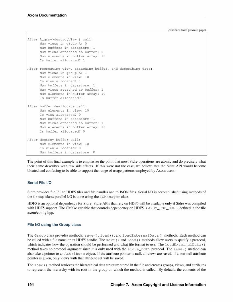
Axom Documentation


After A_grp->destroyView() call:Num views in group A: 0Num buffers in datastore: 1Num views attached to buffer: 0Num elements in buffer array: 10Is buffer allocated? 1

After recreating view, attaching buffer, and describing data:Num views in group A: 1Num elements in view: 10Is view allocated? 1Num buffers in datastore: 1Num views attached to buffer: 1Num elements in buffer array: 10Is buffer allocated? 1

After buffer deallocate call:Num elements in view: 10Is view allocated? 0Num buffers in datastore: 1Num views attached to buffer: 1Num elements in buffer array: 10Is buffer allocated? 0

After destroy buffer call:Num elements in view: 10Is view allocated? 0Num buffers in datastore: 0

The point of this final example is to emphasize the point that most Sidre operations are atomic and do precisely whattheir name describes with few side effects. If this were not the case, we believe that the Sidre API would becomebloated and confusing to be able to support the range of usage patterns employed by Axom users.

Serial File I/O

Sidre provides file I/O to HDF5 files and file handles and to JSON files. Serial I/O is accomplished using methods ofthe Group class; parallel I/O is done using the IOManager class.

HDF5 is an optional dependency for Sidre. Sidre APIs that rely on HDF5 will be available only if Sidre was compiledwith HDF5 support. The CMake variable that controls dependency on HDF5 is AXOM_USE_HDF5, defined in the fileaxom/config.hpp.

File I/O using the Group class

The Group class provides methods: save(), load(), and loadExternalData() methods. Each method canbe called with a file name or an HDF5 handle. The save() and load() methods allow users to specify a protocol,which indicates how the operation should be performed and what file format to use. The loadExternalData()method takes no protocol argument since it is only used with the sidre_hdf5 protocol. The save() method canalso take a pointer to an Attribute object. If the attribute pointer is null, all views are saved. If a non-null attributepointer is given, only views with that attribute set will be saved.

The load() method retrieves the hierarchical data structure stored in the file and creates groups, views, and attributesto represent the hierarchy with its root in the group on which the method is called. By default, the contents of the


Axom Documentation

group are destroyed prior to reading the file contents. This can be suppressed by passing a Boolean value of true as thepreserve_contents argument to the load() method, resulting in the current group subtree being merged withthe file contents.

Usage of the save() and load() methods is shown in the following example.

// Save the data store to a file,// saving all Viewsds->getRoot()->save(filename, protocol);// Delete the data hierarchy under the root, then load it from the fileds->getRoot()->load(filename, protocol);Group* additional = ds->getRoot()->createGroup("additional");additional->createGroup("yetanother");// Load another copy of the data store into the "additional" group// without first clearing all its contentsstd::string groupname;additional->load(filename, protocol, true, groupname);

The loadExternalData() method is used to read “external” data from an HDF5 file created with thesidre_hdf5 protocol. This is data referred to by external views. Such views refer to data that is not stored inSidre buffers but in an external data allocation.

Overloads of the save() and load() methods that take HDF5 handles and the loadExternalData() methodare used to implement parallel I/O through the Sidre IOManager class.

Please see Sidre API Documentation for more detailed description of these Group class methods and the Sidre I/Oprotocols that can be used with them.

Parallel File I/O

The Sidre IOManager class provides an interface to manage parallel I/O of hierarchical data managed by Sidre. Itenables the writing of data from parallel runs and can be used for the purposes of restart or visualization.

Introduction

The IOManager class provides parallel I/O services to Sidre. It relies on the fact that Sidre Group and View objectsare capable of saving and loading themselves. The I/O operations provided by those two classes are inherently serial.So the IOManager class coordinates I/O operations of multiple Sidre objects that exist across the MPI ranks of aparallel run.

• The internal details of the I/O of individual Sidre objects are opaque to the IOManager class, which needsonly to make calls to I/O methods in Group and View class methods.

• Sidre data can be written from M ranks to N files (M >= N), and the files can be read to restart a run on M ranks.

• When saving output, a root file is created that contains bookkeeping information that is used to coordinate asubsequent restart read.

• The calling code can also add extra data to the root file to provide metadata that gives necessary instructions tovisualization tools.

Parallel I/O using the IOManager class

A Sidre IOManager object is created with an MPI communicator and provides various overloads of write() andread() methods. These methods save a Group object in parallel to a set of files and read a Group object from



Axom Documentation

existing files. The I/O manager can optionally use the SCR library for scalable I/O management (such as using burstbuffers when available).

In typical usage, a run that calls read() on a certain set of files should be executed on the same number of MPI ranksas the run that created those files with a write() call. However, if using the sidre_hdf5 protocol, there are someusage patterns that do not have this limitation.

A read() call using the sidre_hdf5 protocol will work when called from a greater number of MPI ranks. Ifwrite() was performed on N ranks and read() is called while running on M ranks (M > N), then data will be readinto ranks 0 to N-1, and all ranks higher than N-1 will receive no data.

If the read() method is called using the sidre_hdf5 protocol to read data that was created on a larger number ofranks, this will work only in the case that the data was written in a file-per-processor mode (M ranks to M files). In thiscase, the data in the group being filled with file input will look a bit different than in other usage patterns, since a groupon one rank will end up with data from multiple ranks. An integer scalar view named reduced_input_rankswill be added to the group with the value being the number of ranks that wrote the files. The data from each outputrank will be read into subgroups located at rank_%07d/sidre_input in the input group’s data hierarchy.

Warning: If the read() is called to read data that was created on a larger number of ranks than the current runwith files produced in M-to-N mode (M > N), an error will occur. Support for this type of usage is intended to beadded in the future.

In the following example, an IOManager object is created and used to write the contents of the “root” group inparallel.

First include needed headers.

#include "axom/config.hpp" // for AXOM_USE_HDF5

#include "conduit_blueprint.hpp"

#include "conduit_relay.hpp"

#ifdef AXOM_USE_HDF5#include "conduit_relay_io_hdf5.hpp"

#endif

#include "axom/sidre/core/sidre.hpp"#include "axom/sidre/spio/IOManager.hpp"#include "axom/fmt.hpp"

#include "mpi.h"

Then use IOManager to save in parallel.

/** Contents of the DataStore written to files with IOManager.

*/int num_files = num_output;axom::sidre::IOManager writer(MPI_COMM_WORLD);

const std::string file_name = "out_spio_parallel_write_read";

writer.write(root, num_files, file_name, PROTOCOL, "tree_%07d");

std::string root_name = file_name + ROOT_EXT;


https://github.com/LLNL/scr

Axom Documentation

Loading data in parallel is easy:

/** Create another DataStore that holds nothing but the root group.

*/DataStore* ds2 = new DataStore();

/** Read from the files that were written above.

*/IOManager reader(MPI_COMM_WORLD);

reader.read(ds2->getRoot(), root_name);

IOManager class use

An IOManager object is constructed with an MPI communicator and does I/O operations on all ranks associatedwith that communicator.

The core functionality of the IOManager class is contained in its write() and read() methods.

void write(sidre::DataGroup * group,int num_files,const std::string& file_string,const std::string& protocol);

The write() method is called on each rank and passed a group pointer for its local data. The calling code specifiesthe number of output files, and the I/O manager organizes the output so that each file receives data from a roughlyequal number of ranks. The files containing the data from the group will have names of the format file_string/file_string_*******.suffix, with a 7-digit integer value identifying the files from 0 to num_files-1, and thesuffix indicating the file format according to the protocol argument. Additionally the write() method will producea root file with the name file_string.root that holds bookkeeping data about other files and can also receiveextra user-specified data.

void read(sidre::DataGroup * group,const std::string& root_file);

The read() methods is called in parallel with the root file as an argument. It must be called on a run with the sameprocessor count as the run that called the write() method. The first argument is a pointer to a group that containsno child groups and owns no views. The second argument is the name of the root file; the information in the root fileis used to identify the files that each processor will read to load data into the argument group.

The write() and read()methods above are sufficient to do a restart save/load when the data in the group hierarchyis completely owned by the Sidre data structures. If Sidre is used to manage data that is externally allocated (i.e.,the hiearchy contains external views), the loading procedure requires additional steps to restore data in the sameexternally-allocated state.

First the read() method is called, and the full hierarchy structure of the group is loaded, but no data is allocated forviews identified as external. Then, the calling code can examine the group and allocate data for the external views, asneeded. The View class method setExternalDataPtr() is used to associate the pointer with the view. Oncethis is done, the I/O manager method loadExternalData() can be used to load the data from the file into theuser-allocated arrays.

Below is a code example for loading external data. We assume that this code somehow has knowledge that the rootgroup contains a single external view at the location “fields/external_array” describing an array of doubles. See theSidre API Documentation for details about Group and View class methods to query the Sidre data structures for thistype of information when the code does not have a priori knowledge.



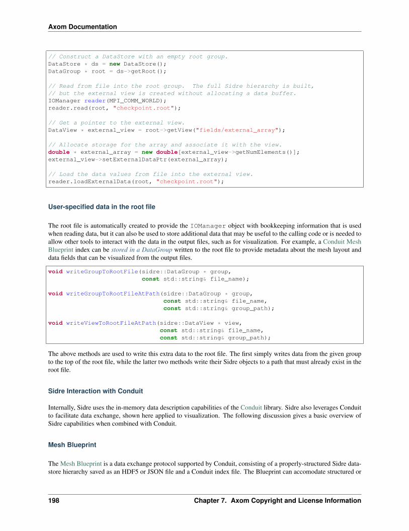
Axom Documentation

// Construct a DataStore with an empty root group.DataStore * ds = new DataStore();DataGroup * root = ds->getRoot();

// Read from file into the root group. The full Sidre hierarchy is built,// but the external view is created without allocating a data buffer.IOManager reader(MPI_COMM_WORLD);reader.read(root, "checkpoint.root");

// Get a pointer to the external view.DataView * external_view = root->getView("fields/external_array");

// Allocate storage for the array and associate it with the view.double * external_array = new double[external_view->getNumElements()];external_view->setExternalDataPtr(external_array);

// Load the data values from file into the external view.reader.loadExternalData(root, "checkpoint.root");

User-specified data in the root file

The root file is automatically created to provide the IOManager object with bookkeeping information that is usedwhen reading data, but it can also be used to store additional data that may be useful to the calling code or is needed toallow other tools to interact with the data in the output files, such as for visualization. For example, a Conduit MeshBlueprint index can be stored in a DataGroup written to the root file to provide metadata about the mesh layout anddata fields that can be visualized from the output files.

void writeGroupToRootFile(sidre::DataGroup * group,const std::string& file_name);

void writeGroupToRootFileAtPath(sidre::DataGroup * group,const std::string& file_name,const std::string& group_path);

void writeViewToRootFileAtPath(sidre::DataView * view,const std::string& file_name,const std::string& group_path);

The above methods are used to write this extra data to the root file. The first simply writes data from the given groupto the top of the root file, while the latter two methods write their Sidre objects to a path that must already exist in theroot file.

Sidre Interaction with Conduit

Internally, Sidre uses the in-memory data description capabilities of the Conduit library. Sidre also leverages Conduitto facilitate data exchange, shown here applied to visualization. The following discussion gives a basic overview ofSidre capabilities when combined with Conduit.

Mesh Blueprint

The Mesh Blueprint is a data exchange protocol supported by Conduit, consisting of a properly-structured Sidre data-store hierarchy saved as an HDF5 or JSON file and a Conduit index file. The Blueprint can accomodate structured or





http://llnl-conduit.readthedocs.io/en/latest/blueprint_mesh.html

Axom Documentation

unstructured meshes, with node- or element-centered fields. The following example shows how to create a Blueprint-conforming datastore hierarchy containing two unstructured adjacent hexahedrons with one node-centered field andone element-centered field. In the diagram, nodes are labeled in black, the node-centered field values are in blue, andthe element-centered field values are in green.

A simulation organizes Sidre data as the code design dictates. Here is a simple example data hierarchy.

Here is the code to create that example data hierarchy.

DataStore* ds = new DataStore();

int nodecount = 12;int elementcount = 2;

// Create views and buffers to hold node positions and field valuesGroup* nodes = ds->getRoot()->createGroup("nodes");View* xs = nodes->createViewAndAllocate("xs", sidre::DOUBLE_ID, nodecount);View* ys = nodes->createViewAndAllocate("ys", sidre::DOUBLE_ID, nodecount);



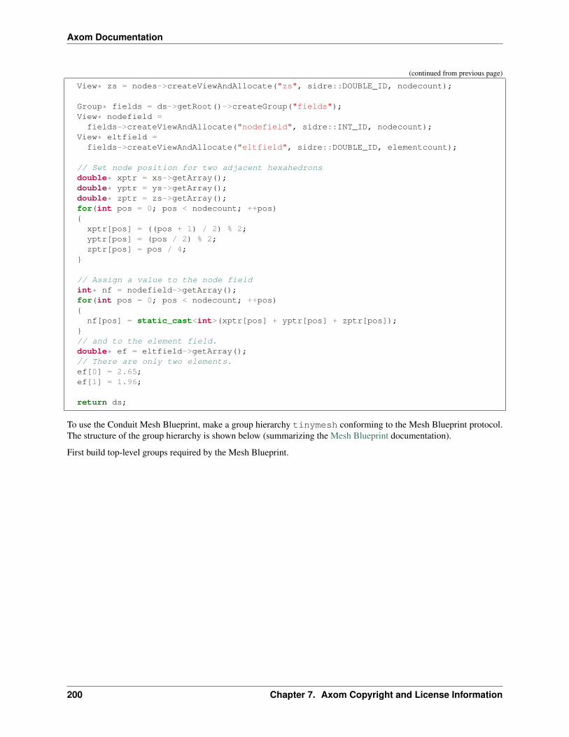
Axom Documentation


View* zs = nodes->createViewAndAllocate("zs", sidre::DOUBLE_ID, nodecount);

Group* fields = ds->getRoot()->createGroup("fields");View* nodefield =fields->createViewAndAllocate("nodefield", sidre::INT_ID, nodecount);

View* eltfield =fields->createViewAndAllocate("eltfield", sidre::DOUBLE_ID, elementcount);

// Set node position for two adjacent hexahedronsdouble* xptr = xs->getArray();double* yptr = ys->getArray();double* zptr = zs->getArray();for(int pos = 0; pos < nodecount; ++pos)xptr[pos] = ((pos + 1) / 2) % 2;yptr[pos] = (pos / 2) % 2;zptr[pos] = pos / 4;

// Assign a value to the node fieldint* nf = nodefield->getArray();for(int pos = 0; pos < nodecount; ++pos)nf[pos] = static_cast<int>(xptr[pos] + yptr[pos] + zptr[pos]);

// and to the element field.double* ef = eltfield->getArray();// There are only two elements.ef[0] = 2.65;ef[1] = 1.96;

return ds;

To use the Conduit Mesh Blueprint, make a group hierarchy tinymesh conforming to the Mesh Blueprint protocol.The structure of the group hierarchy is shown below (summarizing the Mesh Blueprint documentation).

First build top-level groups required by the Mesh Blueprint.



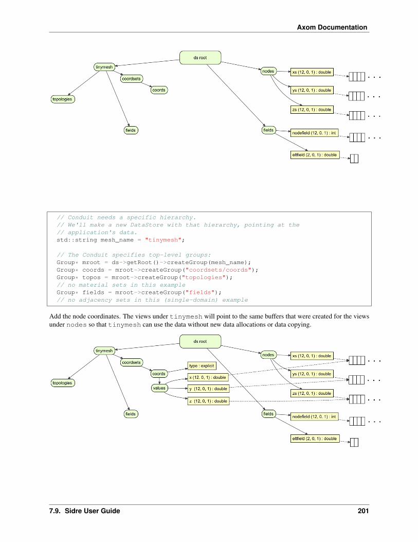
Axom Documentation

// Conduit needs a specific hierarchy.// We'll make a new DataStore with that hierarchy, pointing at the// application's data.std::string mesh_name = "tinymesh";

// The Conduit specifies top-level groups:Group* mroot = ds->getRoot()->createGroup(mesh_name);Group* coords = mroot->createGroup("coordsets/coords");Group* topos = mroot->createGroup("topologies");// no material sets in this exampleGroup* fields = mroot->createGroup("fields");// no adjacency sets in this (single-domain) example

Add the node coordinates. The views under tinymesh will point to the same buffers that were created for the viewsunder nodes so that tinymesh can use the data without new data allocations or data copying.


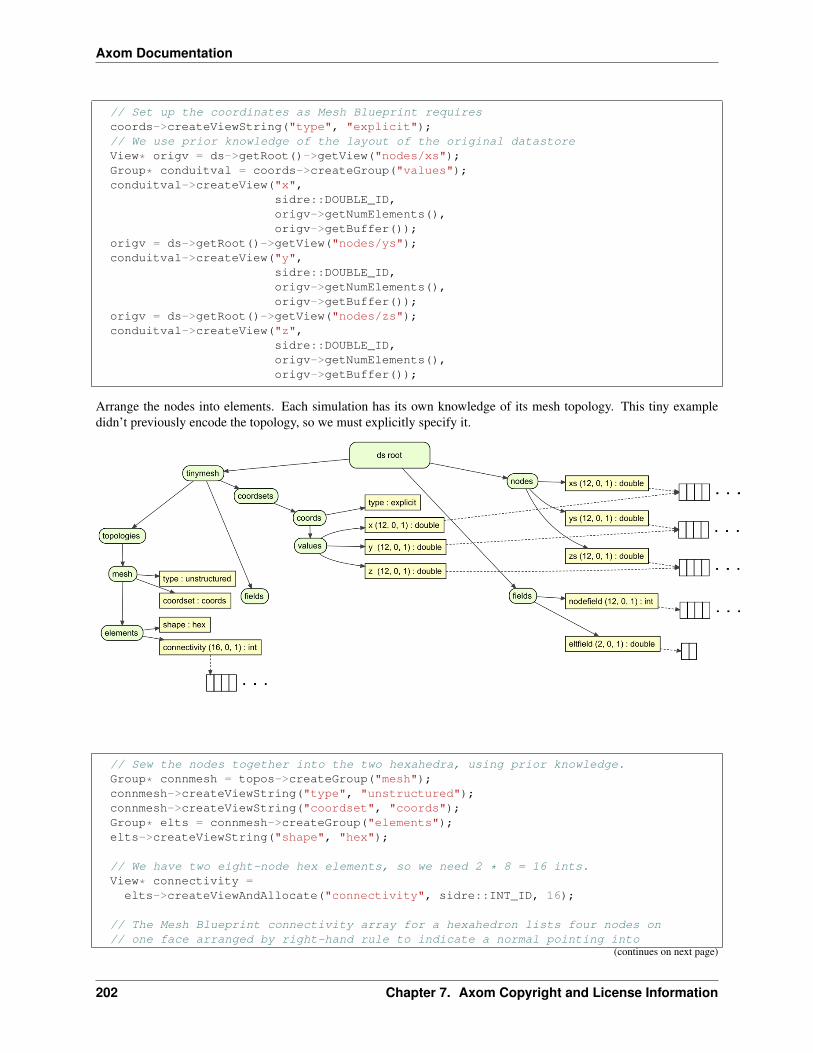
Axom Documentation

// Set up the coordinates as Mesh Blueprint requirescoords->createViewString("type", "explicit");// We use prior knowledge of the layout of the original datastoreView* origv = ds->getRoot()->getView("nodes/xs");Group* conduitval = coords->createGroup("values");conduitval->createView("x",

sidre::DOUBLE_ID,origv->getNumElements(),origv->getBuffer());

origv = ds->getRoot()->getView("nodes/ys");conduitval->createView("y",


origv = ds->getRoot()->getView("nodes/zs");conduitval->createView("z",


Arrange the nodes into elements. Each simulation has its own knowledge of its mesh topology. This tiny exampledidn’t previously encode the topology, so we must explicitly specify it.

// Sew the nodes together into the two hexahedra, using prior knowledge.Group* connmesh = topos->createGroup("mesh");connmesh->createViewString("type", "unstructured");connmesh->createViewString("coordset", "coords");Group* elts = connmesh->createGroup("elements");elts->createViewString("shape", "hex");

// We have two eight-node hex elements, so we need 2 * 8 = 16 ints.View* connectivity =elts->createViewAndAllocate("connectivity", sidre::INT_ID, 16);

// The Mesh Blueprint connectivity array for a hexahedron lists four nodes on// one face arranged by right-hand rule to indicate a normal pointing into



Axom Documentation


// the element, then the four nodes of the opposite face arranged to point// the normal the same way (out of the element). This is the same as for// a VTK_HEXAHEDRON. See// https://www.vtk.org/wp-content/uploads/2015/04/file-formats.pdf.

int* c = connectivity->getArray();

// First hex. In this example, the Blueprint node ordering matches the// dataset layout. This is fortuitous but not required.c[0] = 0;c[1] = 1;c[2] = 2;c[3] = 3;c[4] = 4;c[5] = 5;c[6] = 6;c[7] = 7;

// Second and last hexc[8] = 4;c[9] = 5;c[10] = 6;c[11] = 7;c[12] = 8;c[13] = 9;c[14] = 10;c[15] = 11;

Link the fields into tinymesh. As with the node positions, the views point to the existing buffers containing the fielddata.

// Set up the node-centered field// Get the original dataView* origv = ds->getRoot()->getView("fields/nodefield");Group* nodefield = fields->createGroup("nodefield");



Axom Documentation


nodefield->createViewString("association", "vertex");nodefield->createViewString("type", "scalar");nodefield->createViewString("topology", "mesh");nodefield->createView("values",

sidre::INT_ID,origv->getNumElements(),origv->getBuffer());

// Set up the element-centered field// Get the original dataorigv = ds->getRoot()->getView("fields/eltfield");Group* eltfield = fields->createGroup("eltfield");eltfield->createViewString("association", "element");eltfield->createViewString("type", "scalar");eltfield->createViewString("topology", "mesh");eltfield->createView("values",


Conduit includes a verify method to test if the structure of the tinymesh conforms to the Mesh Blueprint. Thisis valuable for writing and debugging data adapters. Once the datastore hierarchy is properly structured, save it, thenuse Conduit to save the index file (ending with .root). This toy data set is small enough that we can choose to save itin a JSON format.

conduit::Node info, mesh_node, root_node;ds->getRoot()->createNativeLayout(mesh_node);std::string bp_protocol = "mesh";if(conduit::blueprint::verify(bp_protocol, mesh_node[mesh_name], info))// Generate the Conduit indexconduit::Node& index = root_node["blueprint_index"];conduit::blueprint::mesh::generate_index(mesh_node[mesh_name],

mesh_name,1,index[mesh_name]);

std::string root_output_path = mesh_name + ".root";std::string output_path = mesh_name + ".json";

root_node["protocol/name"] = "json";root_node["protocol/version"] = "0.1";root_node["number_of_files"] = 1;root_node["number_of_trees"] = 1;root_node["file_pattern"] = output_path;root_node["tree_pattern"] = "/";

// Now save both the index and the data setconduit::relay::io::save(root_node, root_output_path, "json");conduit::relay::io::save(mesh_node, output_path, "json");

elsestd::cout << "does not conform to Mesh Blueprint: ";info.print();std::cout << std::endl;


Axom Documentation

The code listed above produces the files tinymesh.json and tinymesh.root. Any code that uses Mesh Blueprint can openand use this pair of files.

The DataStore also contains a method that can automatically generate the Blueprint index within a Sidre group ratherthan calling directly into Conduit. Set up a mesh similarly to the example above.

// Conduit needs a specific hierarchy.// We'll make a new Group with that hierarchy, pointing at the// application's data.std::string domain_name = "domain";std::string domain_location = "domain_data/" + domain_name;std::string mesh_name = "mesh";std::string domain_mesh = domain_location + "/" + mesh_name;

Group* mroot = ds->getRoot()->createGroup(domain_location);Group* coords = mroot->createGroup(mesh_name + "/coordsets/coords");Group* topos = mroot->createGroup(mesh_name + "/topologies");// no material sets in this exampleGroup* fields = mroot->createGroup(mesh_name + "/fields");// no adjacency sets in this (single-domain) example

Then call the DataStore::generateBlueprintIndex() method to generate the index within a group in thedatastore. Additional data needed in the root file can be added and saved using Sidre I/O calls.

conduit::Node info, mesh_node, root_node;ds->getRoot()->createNativeLayout(mesh_node);std::string bp_protocol = "mesh";if(conduit::blueprint::verify(bp_protocol, mesh_node[domain_mesh], info))std::string bp("rootfile_data/blueprint_index/automesh");

ds->generateBlueprintIndex(domain_mesh, mesh_name, bp, 1);

Group* rootfile_grp = ds->getRoot()->getGroup("rootfile_data");rootfile_grp->createViewString("protocol/name", "json");rootfile_grp->createViewString("protocol/version", "0.1");rootfile_grp->createViewScalar("number_of_files", 1);rootfile_grp->createViewScalar("number_of_trees", 1);rootfile_grp->createViewScalar("file_pattern", "bpgen.json");rootfile_grp->createViewScalar("tree_pattern", "/domain");rootfile_grp->save("bpgen.root", "json");

ds->getRoot()->getGroup("domain_data")->save("bpgen.json", "json");elsestd::cout << "does not conform to Mesh Blueprint: ";info.print();std::cout << std::endl;

Additionally, the Sidre Parallel I/O (SPIO) class IOManager provides a method that both generates a Blueprint indexand adds it to a root file. Using the same mesh data from the last example, first write out all of the parallel data using theIOManager::write() method. This will output to files all of the data for all domains, and will also create a basicroot file. Then the IOManager::writeBlueprintIndexToRootFile() methods can be called to generatethe Blueprint index and add it to the root file. This is currently only implemented to work with the sidre_hdf5 I/Oprotocol.


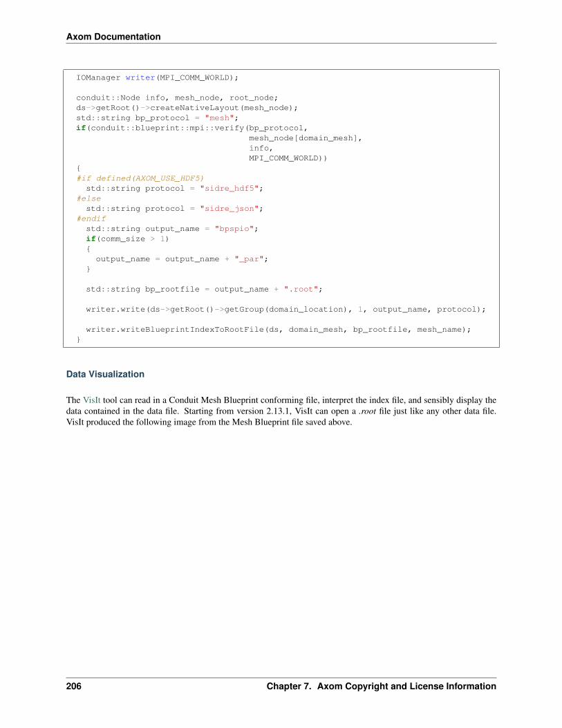
Axom Documentation

IOManager writer(MPI_COMM_WORLD);

conduit::Node info, mesh_node, root_node;ds->getRoot()->createNativeLayout(mesh_node);std::string bp_protocol = "mesh";if(conduit::blueprint::mpi::verify(bp_protocol,

mesh_node[domain_mesh],info,MPI_COMM_WORLD))

#if defined(AXOM_USE_HDF5)std::string protocol = "sidre_hdf5";

#elsestd::string protocol = "sidre_json";

#endifstd::string output_name = "bpspio";if(comm_size > 1)

output_name = output_name + "_par";

std::string bp_rootfile = output_name + ".root";

writer.write(ds->getRoot()->getGroup(domain_location), 1, output_name, protocol);

writer.writeBlueprintIndexToRootFile(ds, domain_mesh, bp_rootfile, mesh_name);

Data Visualization

The VisIt tool can read in a Conduit Mesh Blueprint conforming file, interpret the index file, and sensibly display thedata contained in the data file. Starting from version 2.13.1, VisIt can open a .root file just like any other data file.VisIt produced the following image from the Mesh Blueprint file saved above.


http://visitusers.org/

Axom Documentation

Conduit is also a foundational building block for the Ascent project, which provides a powerful in situ data analyticsand visualization facility (without copying memory) to distributed-memory simulation codes.

Using Sidre with MFEM

Note: The functionality described in this page is only available if Axom is configured with MFEM and if the CMakevariable AXOM_ENABLE_MFEM_SIDRE_DATACOLLECTION is set to ON

The MFEMSidreDataCollection class implements MFEM’s DataCollection interface for recording simu-lation data. Specifically, it knows about fields (mfem::GridFunction objects) and the mesh on which these fieldsare defined.

The MFEMSidreDataCollection class internally organizes its data according to the Mesh Blueprint, a hierarchi-cal schema for describing mesh data.

See the Conduit page for more information on the Mesh Blueprint.

In this page, we first discuss ‘Getting Started‘_ and how MFEM objects can be associated with theMFEMSidreDataCollection. We then explain the process and options available when Saving Data to a File.


http://ascent.readthedocs.io/

https://mfem.org

Axom Documentation

The workflow for reading saved data back in is discussed in Restarting a Simulation.

Associating MFEM Objects with an MFEMSidreDataCollection

We begin to describe the data in an MFEMSidreDataCollection object by registering an MFEM mesh with aninstance of the class when we create the data collection:

// Initialize the datacollection with the mesh// Note: all fields (added with RegisterField) must be on this meshaxom::sidre::MFEMSidreDataCollection dc("sidre_mfem_datacoll_vis_ex", mesh);

The MFEM mesh can also be registered after construction:

dc.SetMesh(/* mfem::Mesh* */ mesh);

Note: There is a 1-1 relationship between MFEMSidreDataCollection objects and MFEM meshes. That is,multiple meshes cannot be associated with a single MFEMSidreDataCollection.

After a mesh has been registered, fields can be association with the MFEMSidreDataCollection object:

// Note: Any number of fields can be registereddc.RegisterField("solution", &soln);

Special kinds of fields (material-dependent fields, material set volume fraction fields, and species set values fields)require additional setup before they can be registered - see Mixed-material Fields for more informantion.

Saving Data to a File

The data in an instance of the MFEMSidreDataCollection class can be saved to a file using a variety of protocols.These files can be visualized with tools like VisIt or used to restart a simulation by loading them back into an instanceof the MFEMSidreDataCollection class (see Restarting a Simulation).

Current options for output protocols/formats include:

• sidre_hdf5

• sidre_conduit_json

• sidre_json

• conduit_hdf5

Note: The AXOM_USE_HDF5 CMake build option must be enabled to use HDF5-based formats.

Before saving, simulation state metadata should be updated. Currently, this metadata consists of:

• cycle, the current iteration number for the simulation

• time, the current simulation time

• time_step, the current simulation time step (sometimes called dt)

Each of these variables has a corresponding setter function:



Axom Documentation

// Save the initial statedc.SetCycle(0); // Iteration counterdc.SetTime(0.0); // Simulation timedc.SetTimeStep(dt); // Time step

Note: There are also corresponding accessors for these state quantities (GetCycle, GetTime, GetTimeStep).

Once state information has been updated, the complete simulation state can be written to a file:

// Filename and protocol, both of which are optionaldc.Save("sidre_mfem_datacoll_vis_ex", sidre_protocol);

Note: By default, saved files will be written to the current working directory. To write to/read from a differentdirectory, use SetPrefixPath to change the directory location of where the MFEMSidreDataCollectionobject’s data will be written.

See the sidre_mfem_datacollection_vis example for a more thorough example of the above functionality.

Restarting a Simulation

Experimental support for complete reconstruction of a simulation mesh, fields, and qfields is also pro-vided by the MFEMSidreDataCollection class. That is, when an output file is read in using theMFEMSidreDataCollection::Load() method, the data read in will be used to reconstruct MFEM objectsthan can be accessed with the GetField, GetQField, and GetMesh methods.

Warning: Currently, an MFEMSidreDataCollection object must own the mesh and field data in order tocompletely reconstruct simulation state. Mesh data ownership can be configured with the owns_mesh_dataconstructor option (should be set to true), and field data ownership requires that each GridFunction objectbe unallocated when passed to the RegisterField() method, which performs the allocation within Sidre-owned memory. After registration, a GridFunction object can be used normally. The same conditions applyfor QuadratureFunction objects.

A complete demonstration of functionality is provided in the sidre_mfem_datacollection_restart exam-ple, which is a stripped-down example of how a simulation code might utilize the automatic reconstruction logic whenloading in a datastore.

Note: The mesh/field reconstruction logic requires that the saved file was created with anMFEMSidreDataCollection object. In Mesh Blueprint terms, the following constraints are imposed onthe structure of the data:

• There must be a coordinate set named coords

• There must be a topology named mesh with corresponding attributes stored in a field namedmesh_material_attribute

• There must be a topology named boundary with corresponding attributes stored in a field namedboundary_material_attribute



Axom Documentation

Mixed-material Fields

The Mesh Blueprint provides support for mixed-material simulations through its material set construct. Materialmetadata (stored in mfem::GridFunction objects) can be registered with the MFEMSidreDataCollectionlike any other field (with the RegisterField() method), given that some additional setup is performed and thefield names match a specific naming convention.

Currently, there are three kinds of special fields that can be associated with mixed-material metadata:

• Volume fraction fields in a material set (the per-element volume fraction of a given material)

• Material-dependent fields (a different set of values for each material)

• Species set fields (a different set of values for each material and for each dimension)

Material sets are defined by associating a volume fraction field name with a material set name:

// Inform the DataCollection that volume fraction information for a material set// called "matset" will be in fields called "volume_fraction"dc.AssociateMaterialSet("volume_fraction", "matset");

Once this association has been made, corresponding fields can be registered. Their names must follow the format<associated volume fraction field name>_<material id>, for example:

dc.RegisterField("volume_fraction_001", vol_frac_1);dc.RegisterField("volume_fraction_002", vol_frac_2);

Material-dependent fields are defined by associating a field name with a material set name:

// Inform the DataCollection of a material-dependent field "density" associated// with a material set called "matset"dc.AssociateMaterialDependentField("density", "matset");

Material-specific values can be registered with a name in the format <associated dependent fieldname>_<material id>:

dc.RegisterField("density", density_independent);dc.RegisterField("density_001", density_dependent_1);dc.RegisterField("density_002", density_dependent_2);

Species sets are defined by associating a field name with a species set name and corresponding material set name:

// Inform the DataCollection that species set data for the species set "specset"// associated with material set "matset" will be in fields called "partial_density"constexpr bool volume_dependent = false;dc.AssociateSpeciesSet("partial_density", "specset", "matset", volume_dependent);

Species set values can be registered with the name in the format <associated field name>_<materialid>_<component>:

dc.RegisterField("partial_density_001_001", partial_density_1_1);dc.RegisterField("partial_density_001_002", partial_density_1_2);dc.RegisterField("partial_density_002_001", partial_density_2_1);dc.RegisterField("partial_density_002_002", partial_density_2_2);


https://llnl-conduit.readthedocs.io/en/latest/blueprint_mesh.html#material-sets

https://llnl-conduit.readthedocs.io/en/latest/blueprint_mesh.html#fields

https://llnl-conduit.readthedocs.io/en/latest/blueprint_mesh.html#species-sets

Axom Documentation

7.10 Slam User Guide

Axom’s Set-theoretic Lightweight API for Meshes (SLAM) component provides high performance building blocksfor distributed-memory mesh data structures in HPC simulation codes.



7.10.2 Introduction

Simulation codes have a broad range of requirements for their mesh data structures, spanning the complexity gamutfrom structured Cartesian grids to fully unstructured polyhedral meshes. Codes also need to support features likedynamic topology changes, adaptive mesh refinement (AMR), submesh elements and ghost/halo layers, in addition toother custom features.

Slam targets the low level implementation of these distributed mesh data structures and is aimed at developers whoimplement mesh data structures within HPC applications.

7.10.3 Set-theoretic abstraction

Slam’s design is motivated by the observation that despite vast differences in the high level features of such mesh datastructures, many of the core concepts are shared at a lower level, where we need to define and process mesh entitiesand their associated data and relationships.

Slam provides a simple, intuitive, API centered around a set-theoretic abstraction for meshes and associated data.Specifically, it models three core set-theoretic concepts:

• Sets of entities (e.g. vertices, cells, domains)

• Relations among a pair of sets (e.g. incidence, adjacency and containment relations)

• Maps defining fields and attributes on the elements of a given set.

The goal is for users to program against Slam’s interface without having to be aware of different design choices, suchas the memory layout and underlying data containers. The exposed API is intended to feel natural to end users (e.g.application developers and domain scientists) who operate on the meshes that are built up from Slam’s abstractions.

See Core concepts for more details.

7.10.4 Policy-based design

There is considerable variability in how these abstractions can be implemented and user codes make many differentdesign choices. For example, we often need different data structures to support dynamic meshes than we do for staticmeshes. Similarly, codes might choose different container types for their arrays (e.g. STL vectors vs. raw C-arrays vs.custom array types).

Performance considerations can also come in to play. For example, in some cases, a code has knowledge of somefixed parameters (e.g. the stride between elements in a relation). Specifying this information at compile-time allowsthe compiler to better optimize the generated code than specifying it at runtime.

Slam uses a Policy-based design to orthogonally decompose the feature space without sacrificing performance. Thismakes it easier to customize the behavior of Slam’s sets, relations and maps and to extend support for custom featuresextend the basic interface.

7.10. Slam User Guide 211

../../../../doxygen/html/slamtop.html

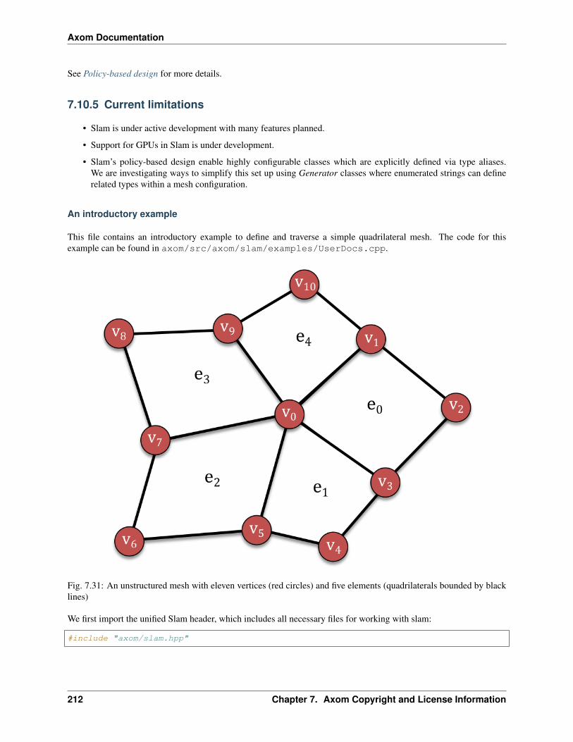
Axom Documentation

See Policy-based design for more details.

7.10.5 Current limitations

• Slam is under active development with many features planned.

• Support for GPUs in Slam is under development.

• Slam’s policy-based design enable highly configurable classes which are explicitly defined via type aliases.We are investigating ways to simplify this set up using Generator classes where enumerated strings can definerelated types within a mesh configuration.

An introductory example

This file contains an introductory example to define and traverse a simple quadrilateral mesh. The code for thisexample can be found in axom/src/axom/slam/examples/UserDocs.cpp.

Fig. 7.31: An unstructured mesh with eleven vertices (red circles) and five elements (quadrilaterals bounded by blacklines)

We first import the unified Slam header, which includes all necessary files for working with slam:

#include "axom/slam.hpp"


Axom Documentation

Note: All code in slam is in the axom::slam namespace. For convenience, we add the following namespacedeclaration to our example to allow us to directly use the slam namespace:

namespace slam = axom::slam;

Type aliases and variables

We begin by defining some type aliases for the Sets, Relations and Maps in our mesh. These type aliases wouldtypically be found in a configuration file or in class header files.

We use the following types throughout this example:

using ArrayIndir = slam::policies::ArrayIndirection<PosType, ElemType>;

Sets

Our mesh is defined in terms of two sets: Vertices and Elements, whose entities are referenced by integer-valuedindices. Since both sets use a contiguous range of indices starting from 0, we use slam::PositionSet to representthem.

We define the following type aliases:

using PosType = slam::DefaultPositionType;using ElemType = slam::DefaultElementType;using VertSet = slam::PositionSet<PosType, ElemType>;using ElemSet = slam::PositionSet<PosType, ElemType>;

and declare them as:

VertSet verts; // The set of vertices in the meshElemSet elems; // The set of elements in the mesh

For other available set types, see Set.

Relations

We also have relations describing the incidences between the mesh vertices and elements.

The element-to-vertex boundary relation encodes the indices of the vertices in the boundary of each element.Since this is a quad mesh and there are always four vertices in the boundary of a quadrilateral, we use aConstantCardinality policy with a CompileTimeStride set to 4 for this StaticRelation.

// Type aliases for element-to-vertex boundary relationenumVertsPerElem = 4

;using CTStride = slam::policies::CompileTimeStride<PosType, VertsPerElem>;using ConstCard = slam::policies::ConstantCardinality<PosType, CTStride>;using ElemToVertRelation =slam::StaticRelation<PosType, ElemType, ConstCard, ArrayIndir, ElemSet, VertSet>;


Axom Documentation

The vertex-to-element coboundary relation encodes the indices of all elements incident in each of the vertices. Sincethe cardinality of this relation changes for different vertices, we use a VariableCardinality policy for thisStaticRelation.

// Type aliases for vertex-to-element coboundary relationusing VarCard = slam::policies::VariableCardinality<PosType, ArrayIndir>;using VertToElemRelation =slam::StaticRelation<PosType, ElemType, VarCard, ArrayIndir, VertSet, ElemSet>;

We declare them as:

ElemToVertRelation bdry; // Boundary relation from elements to verticesVertToElemRelation cobdry; // Coboundary relation from vertices to elements

For other available set types, see Relation.

Maps

Finally, we have some maps that attach data to our sets.

The following defines a type alias for the positions of the mesh vertices. It is templated on a point type (Point2) thathandles simple operations on 2D points.

using BaseSet = slam::Set<PosType, ElemType>;using ScalarMap = slam::Map<BaseSet, Point2>;using PointMap = slam::Map<BaseSet, Point2>;using VertPositions = PointMap;

It is declared as:

VertPositions position; // vertex position

Constructing the mesh

This example uses a very simple fixed mesh, which is assumed to not change after it has been initialized.

Sets

The sets are created using a constructor that takes the number of elements.

verts = VertSet(11); // Construct vertex set with 11 verticeselems = ElemSet(5); // Construct the element set with 5 elements

The values of the vertex indices range from 0 to verts.size()-1 (and similarly for elems).

Note: All sets, relations and maps in Slam have internal validity checks using the isValid() function:

SLIC_ASSERT_MSG(verts.isValid(), "Vertex set is not valid.");SLIC_ASSERT_MSG(elems.isValid(), "Elment set is not valid.");


Axom Documentation

Relations

The relations are constructed by binding their associated sets and arrays of data to the relation instance. In this example,we use an internal helper class RelationBuilder.

We construct the boundary relation by attaching its two sets (elems for its fromSet and verts for its toSet) andan array of indices for the relation’s data.

// construct boundary relation from elements to verticesusing RelationBuilder = ElemToVertRelation::RelationBuilder;bdry = RelationBuilder().fromSet(&elems).toSet(&verts).indices(

RelationBuilder::IndicesSetBuilder().size(static_cast<int>(evInds.size())).data(evInds.data()));

The Coboundary relation requires an additional array of offsets (begins) to indicate the starting index in the relationfor each vertex:

// construct coboundary relation from vertices to elementsusing RelationBuilder = VertToElemRelation::RelationBuilder;cobdry = RelationBuilder()

.fromSet(&verts)

.toSet(&elems)

.begins(RelationBuilder::BeginsSetBuilder().size(verts.size()).data(veBegins.data()))

.indices(RelationBuilder::IndicesSetBuilder().size(static_cast<int>(veInds.size())).data(veInds.data()));

Since these are static relations, we used data that was constructed elsewhere. Note that these relations are lightweightwrappers over the underlying data – no data is copied. To iteratively build the relations, we would use theDynamicConstantRelation and DynamicVariableRelation classes.

See Simplifying mesh setup for more details about Slam’s Builder classes for sets, relations and maps.

Maps

We define the positions of the mesh vertices as a Map on the verts set. For this example, we set the first vertex to lieat the origin, and the remaining vertices line within an annulus around the unit circle.

// construct the position map on the verticesposition = VertPositions(&verts);

// first vertex is at originposition[0] = Point2(0., 0.);

// remaining vertices lie within annulus around unit disk// in cw order, starting at angleOffsetconstexpr double rInner = 0.8;constexpr double rOuter = 1.2;constexpr double angleOffset = 0.75;const double N = verts.size() - 1;

for(int i = 1; i < verts.size(); ++i)



Axom Documentation


const double angle = -(i - 1) / N * 2 * M_PI + angleOffset;const double mag = axom::utilities::random_real(rInner, rOuter);

position[i] = Point2(mag * std::cos(angle), mag * std::sin(angle));

Traversing the mesh

Now that we’ve constructed the mesh, we can start traversing the mesh connectivity and attaching more fields.

Computing a derived field

Our first traversal loops through the vertices and computes a derived field on the position map. For each vertex, wecompute its distance to the origin.

// Create a Map of scalars over the verticesScalarMap distances(&verts);

for(int i = 0; i < distances.size(); ++i) // <-- Map::size()

auto vID = verts[i]; // <-- Set::operator[]const Point2& pt = position[vID]; // <-- Map::operator[]

distances[i] = std::sqrt(pt[0] * pt[0] // <-- Map::operator[]+ pt[1] * pt[1]);

Computing element centroids

Our next example uses element-to-vertex boundary relation to compute the centroids of each element as the averageof its vertex positions.

// Create a Map of Point2 over the mesh elementsusing ElemCentroidMap = PointMap;ElemCentroidMap centroid = ElemCentroidMap(&elems);

// for each element...for(int eID = 0; eID < elems.size(); ++eID) // <-- Set::size()

Point2 ctr;

auto elVerts = bdry[eID]; // <-- Relation::operator[]

// find average position of incident verticesfor(int i = 0; i < elVerts.size(); ++i) // <-- Set::size()

auto vID = elVerts[i]; // <-- Set::operator[]ctr += position[vID]; // <-- Map::operator[]

ctr /= elVerts.size(); // <-- Set::size())centroid[eID] = ctr; // <-- Map::operator[]


Axom Documentation

Perhaps the most interesting line here is when we call the relation’s subscript operator (bdry[eID]). This functiontakes an element index (eID) and returns the set of vertices that are incident in this element. As such, we can use allfunctions in the Set API on this return type, e.g. size() and the subscript operator.

Outputting mesh to disk

As a final example, we highlight several different ways to iterate through the mesh’s Sets, Relations and Maps as weoutput the mesh to disk (in the vtk format).

This is a longer example, but the callouts (left-aligned comments of the form // <-- message ) point to differentiteration patterns.

std::ofstream meshfile;meshfile.open("quadMesh.vtk");std::ostream_iterator<PosType> out_it(meshfile, " ");

// write headermeshfile << "# vtk DataFile Version 3.0\n"

<< "vtk output\n"<< "ASCII\n"<< "DATASET UNSTRUCTURED_GRID\n\n"<< "POINTS " << verts.size() << " double\n";

// write positionsfor(auto pos : position) // <-- Uses range-based for on position map

meshfile << pos[0] << " " << pos[1] << " 0\n";

// write elem-to-vert boundary relationmeshfile << "\nCELLS " << elems.size() << " " << 5 * elems.size();for(auto e : elems) // <-- uses range-based for on element set

meshfile << "\n4 ";std::copy(bdry.begin(e), // <-- uses relation's iterators

bdry.end(e),out_it);

// write element types ( 9 == VKT_QUAD )meshfile << "\n\nCELL_TYPES " << elems.size() << "\n";for(int i = 0; i < elems.size(); ++i)

meshfile << "9 ";

// write element idsmeshfile << "\n\nCELL_DATA " << elems.size() << "\nSCALARS cellIds int 1"

<< "\nLOOKUP_TABLE default \n";for(int i = 0; i < elems.size(); ++i)

meshfile << elems[i] << " "; // <-- uses size() and operator[] on set

// write vertex idsmeshfile << "\n\nPOINT_DATA " << verts.size() << "\nSCALARS vertIds int 1"

<< "\nLOOKUP_TABLE default \n";(continues on next page)


Axom Documentation


for(int i = 0; i < verts.size(); ++i)

meshfile << verts[i] << " ";meshfile << "\n";

Core concepts

Describe Slam concepts, what they mean, how they are used, etc.

Fig. 7.32: A relation (blue lines) between two sets (ovals with red and green dots, as elements) and a map of scalarvalues (brown) on the second set.

Set

• Taxonomy of set types (OrderedSet, IndirectionSet, Subset, static vs. dynamic)

• Simple API (including semantics of operator[] and iterators )


Axom Documentation

• Example to show how we iterate through a set

Relation

• Relational operator (from element of Set A to set of elements in Set B)

• Taxonomy:

– Cardinality: Fixed vs Variable number of elements per relation

– Mutability: Static vs. Dynamic relation

– Storage: Implicit vs. Explicit (e.g. product set)

• Simple API (including semantics of operator[] )

• Three ways to iterate through a relations

– Double subscript

– Separate subscripts

– Iterators

Map

• Data associated with all members of a set

• Simple API (including semantics of operator[] )

Implementation details

Policy-based design

Handling the combinatorial explosion of features; avoid paying for what we don’t need

• SizePolicy, StridePolicy, OffsetPolicy (compile time vs. runtime)

• IndirectionPolicy (none, C-array, std::vector, custom, e.g. mfem::Array)

• SubsettingPolicy (none, virtual parent, concrete parent)

• OwnershipPolicy (local, sidre, other repository)

Feature diagram of OrderedSet policies (subset).

The figure shows how certain these policies interact with the subscript operator.

Simplifying mesh setup

• Builder classes

– Chained initialization using named-parameter idiom

• Generator classes to simplify types


Axom Documentation

7.11 Slic User Guide

Slic provides a light-weight, modular and extensible logging infrastructure that simplifies logging application mes-sages.



7.11.2 Key Features

• Interoperability across the constituent libraries of an application. Messages logged by an application and any ofits libraries using Slic have a unified format and routed to a centralized output destination.

• Customizable Log Message Format to suit application requirements.

• Customizable handling and filtering of log messages by extending the Log Stream base class.

• Built-In Log Streams to support common logging use cases, e.g., log to a file or console.

• Native integration with Lumberjack for logging and filtering of messages at scale.

• Fortran bindings that provide an idiomatic API for Fortran applications.

7.11.3 Requirements

Slic is designed to be light-weight and self-contained. The only requirement for using Slic is a C++11 compliantcompiler. However, to use Slic in the context of a distributed parallel application and in conjunction with Lumberjack,support for building with MPI is provided.


../../../../doxygen/html/slictop.html

../../../lumberjack/docs/sphinx/index.html

../../../lumberjack/docs/sphinx/index.html

Axom Documentation

For further information on how to build the Axom Toolkit, consult the Axom Quick Start Guide.

7.11.4 About this Guide

This guide presents core concepts, key capabilities, and guiding design principles of Slic’s Component Architecture.To get started with using Slic quickly within an application, see the Getting Started with Slic section. For more detailedinformation on the interfaces of the various classes and functions in Slic, developers are advised to consult the SlicDoxygen API.

Additional questions, feature requests or bug reports on Slic can be submitted by creating a new issue on Github or bysending e-mail to the Axom Developers mailing list at [email protected].

Getting Started with Slic

This section illustrates some of the key concepts and capabilities of Slic by presenting a short walk-through of a C++application. The complete Slic Application Code Example is included in the Appendix section and is also availablewithin the Slic source code, under src/axom/slic/examples/basic/logging.cpp.

This example illustrates the following concepts:

• Initializing the Slic Logging Environment,

• Prescribing the Log Message Format,

• Basic logging to the console using the Generic Output Stream, and,

• Using some of the various Slic Macros Used in Axom to log messages.

Step 1: Add Header Includes

First, the Slic header must be included to make all the Slic functions and classes accessible to an application:

1 // Slic includes2 #include "axom/slic.hpp"

Note: All the classes and functions in Slic are encapsulated within the axom::slic namespace.

Step 2: Initialize Slic

Prior to logging any messages, the Slic Logging Environment is initialized by the following:

1 slic::initialize();

This creates the root logger instance. However, in order to log messages, an application must first specify an outputdestination and optionally, prescribe the format of the log messages. These steps are demonstrated in the followingsections.

Step 3: Set the Message Format

The Log Message Format is specified as a string consisting of keywords, enclosed in < ... >, that Slic knows howto interpret when assembling the log message.

7.11. Slic User Guide 221

../../../../index.html





mailto:[email protected]

Axom Documentation

1 std::string format = std::string("<TIMESTAMP>\n") +2 std::string("[<LEVEL>]: <MESSAGE> \n") + std::string("FILE=<FILE>\n") +3 std::string("LINE=<LINE>\n\n");

For example, the format string in the code snippet above indicates that the resulting log messages will have thefollowing format:

• A line with the message time stamp

• A line consisting of the Log Message Level, enclosed in brackets [ ], followed by the user-supplied message,

• A third line with the name of the file where the message was emitted and

• The corresponding line number location within the file, in the fourth line.

The format string is used in Step 5: Register a Log Stream. Specifically, it is passed as an argument to the GenericOutput Stream object constructor to prescribe the format of the messages.

See the Log Message Format section for the complete list of keyword options available that may be used to customizethe format of the messsages.

Note: This step is optional. If the format is not specified, a Default Message Format will be used to assemble themessage.

Step 4: Set Severity Level

The severity of log messages to be captured may also be adjusted at runtime to the desired Log Message Level bycalling slic::setLoggingMsgLevel(). This provides another knob that the application can use to filter thetype and level of messages to be captured.

All log messages with the specified severity level or higher are captured. For example, the following code snippet setsthe severity level to debug.

1 slic::setLoggingMsgLevel(slic::message::Debug);

This indicates that all log messages that are debug or higher are captured otherwise, the messages are ignored. Sincedebug is the lowest severity level, all messages will be captured in this case.

Step 5: Register a Log Stream

Log messages can have one or more output destination. The output destination is specified by registering a corre-sponding Log Stream object to each Log Message Level.

The following code snippet uses the Generic Output Stream object, one of the Built-In Log Streams provided by Slic,to specify std::cout as the output destination for messages at each Log Message Level.

1 slic::addStreamToAllMsgLevels(new slic::GenericOutputStream(&std::cout, format));

Note: Instead of calling slic::addStreamToAllMsgLevels() an application may useslic::addStreamToMsgLevel() that allows more fine grain control of how to bind Log Stream objectsto each Log Message Level. Consult the Slic Doxygen API Documentation for more information.

The Generic Output Stream, takes two arguments in its constructor:


../../../../../doxygen/html/slictop.html

Axom Documentation

• A C++ std::ostream object that specifies the destination of messages. Consequently, output of mes-sages can be directed to the console, by passing std::cout or std::cerr, or to a file by passing a C++std::ofstream object. In this case, std::cout is specified as the output destination.

• A string corresponding to the Log Message Format, discussed in Step 3: Set the Message Format.

Note: Slic maintains ownership of all registered Log Stream instances and will deallocate them whenslic::finalize() is called.

Step 5: Log Messages

Once the output destination of messages is specified, messages can be logged using the Slic Macros Used in Axom, asdemonstrated in the code snippet below.

1 SLIC_DEBUG("Here is a debug message!");2 SLIC_INFO("Here is an info mesage!");3 SLIC_WARNING("Here is a warning!");4 SLIC_ERROR("Here is an error message!");

Note: By default, SLIC_ERROR() will print the specified message and a stacktrace to the corresponding outputdestination and call axom::utilities::processAbort() to gracefully abort the application. This behavior can be toggledby calling slic::disableAbortOnError(). Additionally, a custom abort function can be registered withslic::setAbortFunction(). See the Slic Doxygen API Documentation for more details.

Step 6: Finalize Slic

Before the application terminates, the Slic Logging Environment must be finalized, as follows:

1 slic::finalize();

Calling slic::finalize() will properly deallocate the registered Log Stream objects and terminate the SlicLogging Environment.

Step 7: Run the Example

After building the Axom Toolkit the Slic Application Code Example may be run from within the build space directoryas follows:

> ./example/slic_logging_ex

The resulting output should look similar to the following:

Fri Apr 26 14:29:53 2019[DEBUG]: Here is a debug message!FILE=/Users/zagaris2/dev/AXOM/source/axom/src/axom/slic/examples/basic/logging.cppLINE=44

Fri Apr 26 14:29:53 2019[INFO]: Here is an info mesage!




../../../../../index.html

Axom Documentation


FILE=/Users/zagaris2/dev/AXOM/source/axom/src/axom/slic/examples/basic/logging.cppLINE=45

Fri Apr 26 14:29:53 2019[WARNING]: Here is a warning!FILE=/Users/zagaris2/dev/AXOM/source/axom/src/axom/slic/examples/basic/logging.cppLINE=46

Fri Apr 26 14:29:53 2019[ERROR]: Here is an error message!

** StackTrace of 3 frames **Frame 1: axom::slic::logErrorMessage(std::__1::basic_string<char, std::__1::char_→˓traits<char>,std::__1::allocator<char> > const&, std::__1::basic_string<char, std::__1::char_traits→˓<char>,std::__1::allocator<char> > const&, int)Frame 2: mainFrame 3: start=====

FILE=/Users/zagaris2/dev/AXOM/source/axom/src/axom/slic/examples/basic/logging.cppLINE=47

Abort trap: 6

Component Architecture

Slic provides a simple and easy to use logging interface for applications.

The basic component architecture of Slic, depicted in Fig. 7.33, consists of three main components:

1. A static logger API. This serves as the primary interface to the application.

2. One or more Logger object instances. In addition to the root logger, which is created when Slic is initialized, anapplication may create additional loggers. However, at any given instance, there is only a single active logger towhich all messages are logged.

• A Logger consists of four log message levels: ERROR, WARNING, INFO and DEBUG.

• Each Log Message Level can have one or more Log Stream instances, which, specify the output destination,format and filtering of messages.

3. One or more Log Stream instances, bound to a particular logger, that can be shared between log message levels.

The application logs messages at an appropriate Log Message Level, i.e., ERROR, WARNING, INFO, or, DEBUG usingthe static API. Internally, the Logger routes the message to the corresponding Log Stream instances that are bound tothe associated Log Message Level.

The following sections discuss some of these concepts in more detail.

Log Message Level

The Log Message Level indicates the severity of a message. Slic provides four levels of messages ranked from highestto lowest as follows:


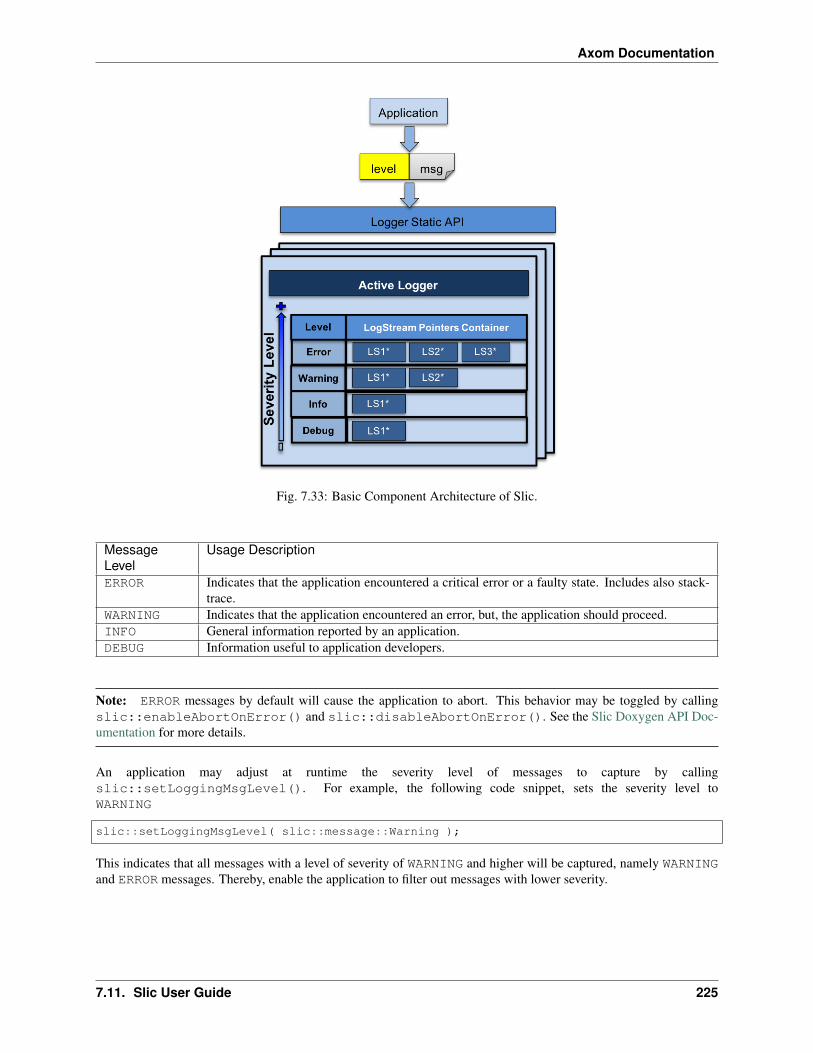
Axom Documentation

Fig. 7.33: Basic Component Architecture of Slic.

MessageLevel

Usage Description

ERROR Indicates that the application encountered a critical error or a faulty state. Includes also stack-trace.

WARNING Indicates that the application encountered an error, but, the application should proceed.INFO General information reported by an application.DEBUG Information useful to application developers.

Note: ERROR messages by default will cause the application to abort. This behavior may be toggled by callingslic::enableAbortOnError() and slic::disableAbortOnError(). See the Slic Doxygen API Doc-umentation for more details.

An application may adjust at runtime the severity level of messages to capture by callingslic::setLoggingMsgLevel(). For example, the following code snippet, sets the severity level toWARNING

slic::setLoggingMsgLevel( slic::message::Warning );

This indicates that all messages with a level of severity of WARNING and higher will be captured, namely WARNINGand ERROR messages. Thereby, enable the application to filter out messages with lower severity.




Axom Documentation

Log Stream

The Log Stream class, is an abstract base class that facilitates the following:

• Specifying the Log Message Format and output destination of log messages.

• Implementing logic for handling and filtering messages.

• Defines a pure abstract interface for all Log Stream instances.

Since Log Stream is an abstract base class, it cannot be instantiated and used directly. Slic provides a set of Built-InLog Streams, which provide concrete implementations of the Log Stream base class that support common use casesfor logging, e.g., logging to a file or output to the console.

Applications requiring custom functionality, may extend the Log Stream class and provide a concrete Log Streaminstance implementation that implements the abstract interface defined by the Log Stream base class. See the Add aCustom Log Stream section for details.

A concrete Log Stream instance can be attached to one or more Log Message Level by callingslic::addStreamToMsgLevel() and slic::addStreamToAllMsgLevels(). See the Slic DoxygenAPI Documentation for more details.

Log Message Format

The Log Message Format is specified as a string consisting of keywords that are encapsulated in <...>, which, Slicknows to interpret when assembling the log message.

The list of keywords is summarized in the table below.

key-word

Replaced With

<TIMES-TAMP>

A textual representation of the time a message is logged, as returned by std::asctime().

<LEVEL>The Log Message Level, i.e., ERROR, WARNING, INFO, or DEBUG.<MES-SAGE>

The supplied message that is being logged.

<FILE> The file from where the message was emmitted.<LINE> The line location where the message was emmitted.<TAG> A string tag associated with a given message, e.g., for filtering during post-processing, etc.<RANK> The MPI rank that emmitted the message. Only applicable when the Axom Toolkit is compiled with

MPI enabled and with MPI-aware Log Stream instances, such as, the Synchronized Output Stream andLumberjack Stream.

These keywords can be combined in a string to specify a template for a log message.

For example, the following code snippet, specifies that all reported log messages consist of the level, enclosed inbrackets followed by the user-supplied log message.

std::string format = "[<LEVEL>]: <MESSAGE>";

To get the file and line location within the file where the message was emitted, the format string above could beamended with the following:

std::string format = "[<LEVEL>]: <MESSAGE> \n\t<FILE>:<LINE>";

This indicates that the in addition to the level and user-supplied, the resulting log messages will have an additional lineconsisting of the file and line where the message was emitted.




../../../../../index.html

Axom Documentation

Default Message Format

If the Log Message Format is not specified, the Log Stream base class defines a default format that is set to thefollowing:

std::string DEFAULT_FORMAT = "*****\n[<LEVEL>]\n\n <MESSAGE> \n\n <FILE>\n<LINE>→˓\n****\n"

Built-In Log Streams

The Built-In Log Streams provided by Slic are summarized in the following table, followed by a brief description foreach.

Log Stream Use & AvailabilityGeneric Output Stream Always available. Used in serial applications, or, for logging on rank zero.Synchronized Output Stream Requires MPI. Used with MPI applications.Lumberjack Stream Requires MPI. Used with MPI applications.

Generic Output Stream

The Generic Output Stream, is a concrete implementation of the Log Stream base class, that can be constructed byspecifying:

1. A C++ std::ostream object instance, e.g., std::cout`, ``std::cerr for console output, or to a fileby passing a C++ std::ofstream object, and,

2. Optionally, a string that specifies the Log Message Format.

For example, the following code snippet registers a Generic Output Stream object that is bound to the the std::cout.

slic::addStreamToAllMsgLevels(new slic::GenericOutputStream( &std::cout, format ) );

Similarly, the following code snippet, registers a Generic Output Stream object that is bound to a file.

std::ofstream log_file;log_file.open( "logfile.dat" );

slic::addStreamToAllMsgLevels(new slic::GenericOutputStream( &log_file, format ) );

Synchronized Output Stream

The Synchronized Output Stream is intended to be used with parallel MPI applications, primarily for debugging. TheSynchronized Output Stream provides similar functionality to the Generic Output Stream, however, the log messagesare synchronized across the MPI ranks of the specified communicator.

Similar to the Generic Output Stream the Synchronized Output Stream is constructed by specifying:

1. A C++ std::ostream object instance, e.g., std::cout`, ``std::cerr for console output, or to a fileby passing a C++ std::ofstream object.

2. The MPI communicator, and,


Axom Documentation


The following code snippet illustrates how to register a Synchronized Output Stream object with Slic to log messagesto std::cout.

slic::addStreamToAllMsgLevels(new slic::SynchronizedOutputStream( &std::cout, mpi_comm, format ) );

Note: Since, the Synchronized Output Stream works across MPI ranks, logging messages using the Slic Macros Usedin Axom or the static API directly only logs the messages locally. To send the messages to the output destination theapplication must call slic::flushStreams() explicitly, which, in this context is a collective call.

Lumberjack Stream

The Lumberjack Stream, is intended to be used with parallel MPI applications. In contrast to the Synchronized OutputStream, which logs messages from all ranks, the Lumberjack Stream uses Lumberjack internally to filter out duplicatemessages that are emitted from multiple ranks.

The Lumberjack Stream is constructed by specifying:

1. A C++ std::ostream object instance, e.g., std::cout`, ``std::cerr for console output, or to a fileby passing a C++ std::ofstream object.

2. The MPI communicator,

3. An integer that sets a limit on the number of duplicate messsages reported per rank, and,


The following code snippet illustrates how to register a Lumberjack Stream object with Slic to log messages tostd::cout.

slic::addStreamToAllMsgLevels(new slic::LumberjackStream( &std::cout, mpi_comm, 5, format ) );

Note: Since, the Lumberjack Stream works across MPI ranks, logging messages using the Slic Macros Used in Axomor the static API directly only logs the messages locally. To send the messages to the output destination the applicationmust call slic::flushStreams() explicitly, which, in this context is a collective call.

Add a Custom Log Stream

Slic can be customized by implementing a new subclass of the Log Stream. This section demonstrates the basic stepsrequired to Add a Custom Log Stream by walking through the implementation of a new Log Stream instance, whichwe will call MyStream.

Note: MyStream provides the same functionality as the Generic Output Stream. The implementation presentedherein is primarily intended for demonstrating the basic process for extending Slic by providing a custom Log Stream.


../../../../lumberjack/docs/sphinx/index.html

Axom Documentation

Create a LogStream Subclass

First, we create a new class, MyStream, that is a subclass of the Log Stream class, as illustrated in the code snippetbelow.

1 class MyStream : public LogStream2 3 public:4

5 MyStream( ) = delete;6 MyStream( std::ostream* os, const std::string& format );7

8 virtual ~MyStream();9

10 /// \see LogStream::append11 virtual void append( message::Level msgLevel,12 const std::string& message,13 const std::string& tagName,14 const std::string& fileName,15 int line,16 bool filter_duplicates );17 private:18 std::ostream* m_stream;19

20 // disable copy & assignment21 MyStream( const MyStream & ) = delete;22 MyStream& operator=(const MyStream&) = delete;23

24 // disable move & assignment25 MyStream( const MyStream&& ) = delete;26 MyStream& operator=(const MyStream&&) = delete;27 ;

The class has a pointer to a C++ std::ostream object as a private class member. The std::ostream ob-ject holds a reference to the output destination for log messages, which can be any std::ostream instance, e.g.,std::cout, std::cerr, or a file std::ofstream, etc.

The reference to the std::ostream is specified in the class constructor and is supplied by the application when aMyStream object is instantiated.

Since MyStream is a concrete instance of the Log Stream base class, it must implement the append() method,which is a pure virtual method.

Implement LogStream::append()

The MyStream class implements the LogStream::append() method of the Log Stream base class, as demon-strated in the code snippet below.

1 void MyStream::append( message::Level msgLevel,2 const std::string& message,3 const std::string& tagName,4 const std::string& fileName,5 int line,6 bool AXOM_UNUSED_PARAM(filtered_duplicates) )7 8 assert( m_stream != nillptr );



Axom Documentation


9

10 (*m_stream) << this->getFormatedMessage( message::getLevelAsString(msgLevel),11 message,12 tagName,13 "",14 fileName,15 line );16

The append() method takes all the metadata associated with a message through its argument list:

• The Log Message Level

• The user-specified message

• A tag associated with the message, may be set MSG_IGNORE_TAG

• The file where the message was emitted

• The line location within the file where the message was emitted

The append() method calls LogStream::getFormatedMessage(), a method implemented in the LogStream base class, which, applies the Log Message Format according to the specified format string supplied to theMyStream class constructor, when the class is instantiated.

Register the new class with Slic

The new Log Stream class may be used with Slic in a similar manner to any of the Built-In Log Streams, as demon-strated in the code snippet below:

slic::addStreamToAllMsgLevels( new MyStream( &std::cout, format ) );

Wrapping Slic in Macros

The recommended way of integrating Slic into an application is to wrap the Slic API for logging messages into a setof convenience application macros that are used throughout the application code.

This allows the application code to:

• Centralize all use of Slic behind a thin macro layer,

• Insulate the application from API changes in Slic,

• Customize and augment the behavior of logging messages if needed, e.g., provide macros that are only activewhen the code is compiled with debug symbols etc.

The primary function used to log messages is slic::logMessage(), which in its most basic form takes thefollowing arguments:

1. The Log Message Level associated with the message

2. A string corresponding to the user-supplied message

3. The name of the file where the message was emitted

4. The corresponding line number within the file where the message was emitted


Axom Documentation

There are additional variants of the slic::logMessage() function that allow an application to specify a TAG fordifferent types of messages, etc. Consult the Slic Doxygen API Documentation for more details.

For example, an application, MYAPP, may want to define macros to log DEBUG, INFO, WARNING and ERROR mes-sages as illustrated below

1 #define MYAPP_LOGMSG( LEVEL, msg ) \2 \3 std::ostringstream oss; \4 oss << msg; \5 slic::logMessage( LEVEL, oss.str(), __FILE__, __LINE__ ); \6 7

8 #define MYAPP_ERROR( msg ) MYAPP_LOGMSG( slic::message::Error, msg )9 #define MYAPP_WARNING( msg ) MYAPP_LOGMSG( slic::message::Warning, msg )

10 #define MYAPP_INFO( msg ) MYAPP_LOGMSG( slic::message::Info, msg )11 #define MYAPP_DEBUG( msg ) MYAPP_LOGMSG( slic::message::Debug, msg )

These macros can then be used in the application code as follows:

MYAPP_INFO( "this is an info message")MYAPP_ERROR( "this is an error message" );...

Note: Another advantage of encapsulating the Slic API calls in macros is that this approach alleviates the burdenfrom application developers to have to pass the __FILE__ and __LINE__ to the logMessage() function eachtime.

The Slic Macros Used in Axom provide a good resource for the type of macros that an application may want to adoptand extend. Although these macros are tailored for use within the Axom Toolkit, these are also callable by applicationcode.

Appendix

Slic Application Code Example

Below is the complete Slic Application Code Example presented in the Getting Started with Slic section. The code canbe found in the Axom source code under src/axom/slic/examples/basic/logging.cpp.

1 // SPHINX_SLIC_INCLUDES_BEGIN2 // Slic includes3 #include "axom/slic.hpp"4 // SPHINX_SLIC_INCLUDES_END5

6 using namespace axom;7

8 //---------------------------------------------------------------------------→˓---

9 int main(int AXOM_UNUSED_PARAM(argc), char** AXOM_UNUSED_PARAM(argv))10 11 // SPHINX_SLIC_INIT_BEGIN




../../../../../index.html

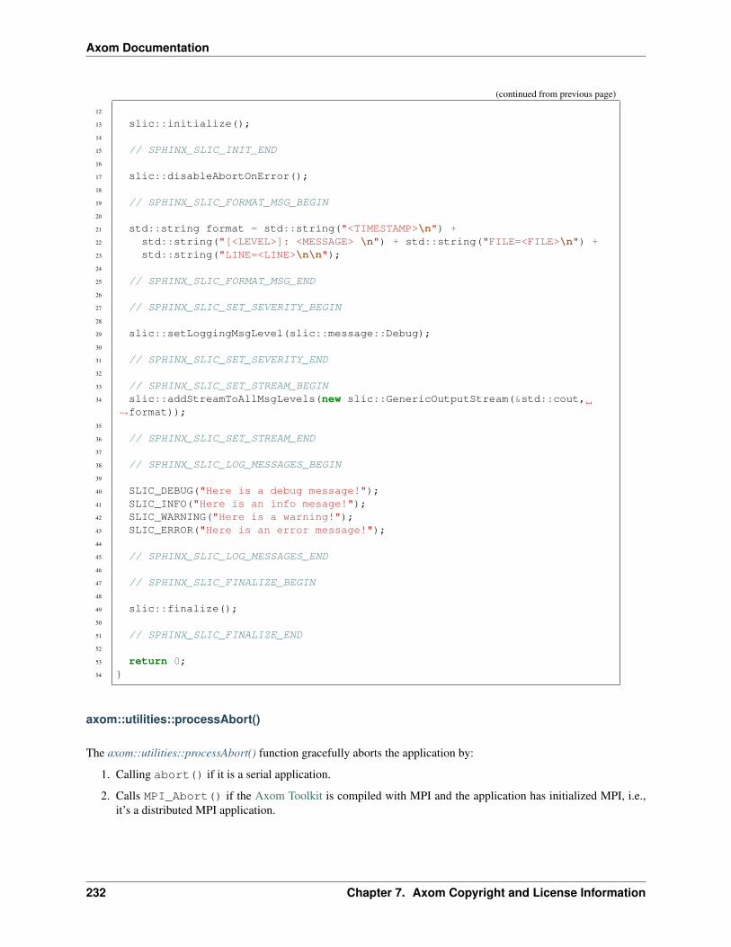
Axom Documentation


12

13 slic::initialize();14

15 // SPHINX_SLIC_INIT_END16

17 slic::disableAbortOnError();18

19 // SPHINX_SLIC_FORMAT_MSG_BEGIN20

21 std::string format = std::string("<TIMESTAMP>\n") +22 std::string("[<LEVEL>]: <MESSAGE> \n") + std::string("FILE=<FILE>\n") +23 std::string("LINE=<LINE>\n\n");24

25 // SPHINX_SLIC_FORMAT_MSG_END26

27 // SPHINX_SLIC_SET_SEVERITY_BEGIN28

29 slic::setLoggingMsgLevel(slic::message::Debug);30

31 // SPHINX_SLIC_SET_SEVERITY_END32

33 // SPHINX_SLIC_SET_STREAM_BEGIN34 slic::addStreamToAllMsgLevels(new slic::GenericOutputStream(&std::cout,

→˓format));35

36 // SPHINX_SLIC_SET_STREAM_END37

38 // SPHINX_SLIC_LOG_MESSAGES_BEGIN39

40 SLIC_DEBUG("Here is a debug message!");41 SLIC_INFO("Here is an info mesage!");42 SLIC_WARNING("Here is a warning!");43 SLIC_ERROR("Here is an error message!");44

45 // SPHINX_SLIC_LOG_MESSAGES_END46

47 // SPHINX_SLIC_FINALIZE_BEGIN48

49 slic::finalize();50

51 // SPHINX_SLIC_FINALIZE_END52

53 return 0;54

axom::utilities::processAbort()

The axom::utilities::processAbort() function gracefully aborts the application by:

1. Calling abort() if it is a serial application.

2. Calls MPI_Abort() if the Axom Toolkit is compiled with MPI and the application has initialized MPI, i.e.,it’s a distributed MPI application.


../../../../../index.html

Axom Documentation

Slic Macros Used in Axom

Slic provides a set of convenience macros that can be used to streamline logging within an application.

Note: The Slic Macros Used in Axom are not the only interface to log messages with Slic. They are used within theAxom Toolkit for convenience. Applications or libraries that adopt Slic, typically, use the C++ API directly, e.g., callslic::logMessage() and wrap the functionality in application specific macros to better suit the requirements ofthe application.

SLIC_INFO

The SLIC_INFO macro logs INFO messages that consist general information reported by an application.

The following code snippet illustrates the usage of the SLIC_INFO macro:

SLIC_INFO( "Total number of mesh cells:" << N );

SLIC_INFO_IF

The SLIC_INFO_IF macro provides the same functionality with the SLIC_INFO macro, however, it takes one ad-ditional argument, a boolean expression, that allows the application to conditionally log an INFO message dependingon the value of the boolean expression.

For example, the following code snippet illustrates the usage of the SLIC_INFO_IF macro.

SLIC_INFO_IF( (myval >= 0), "[" << myval << "] is positive!" );

In this case, the INFO message is only logged when the boolean expression, (myval >=0) evaluates to true.

Note: The primary intent is to provide a convenience layer and facilitate in a cleaner and more compact code style byencapsulating the conditional branching logic within a macro.

SLIC_ERROR

The SLIC_ERROR macro logs ERROR messages that indicate that the application has encountered a critical error.

The following code snippet illustrates the basic usage of the SLIC_ERROR macro:

SLIC_ERROR( "jacobian is negative!" );

A stacktrace of the application is appended to all ERROR messages to facilitate debugging.

Note: By default, an ERROR message triggers a call to abort() the application. However, this behavior can betoggled by calling slic::enableAbortOnError() and slic::disableAbortOnError() accordingly.See the Slic Doxygen API Documentation for more information.


../../../../../index.html


Axom Documentation

SLIC_ERROR_IF

The SLIC_ERROR_IF provides the same functionality with the SLIC_ERROR macro, however, it takes one additionalargument, a boolean expression, that allows the application to conditionally log an ERROR message depending on thevalue of the boolean expression.

The following code snippet illustrates the usage of the SLIC_ERROR_IF macro.

SLIC_ERROR_IF( (jacobian < 0.0 + TOL), "jacobian is negative!" );

In this case, the ERROR message in only logged when the boolean expression, (jacobian < 0.0 + TOL) eval-uates to true.


SLIC_WARNING

The SLIC_WARNING macro logs WARNING messages that indicate that the application has encountered an error,however, the error is not critical and the application can proceed.

The following code snippet illustrates the basic usage of the SLIC_WARNING macro.

SLIC_WARNING( "Region [" << ir << "] defined but not used in the problem!" );

SLIC_WARNING_IF

Similarly, the SLIC_WARNING_IF macro provides the same functionality with the SLIC_WARNING macro, how-ever, it takes one additional argument, a boolean expression, that allows the application to conditionally log aWARNING message depending on the value of the boolean expression.

The following code snippet illustrates the basic usage of the SLIC_WARNING_IF macro.

SLIC_WARNING_IF( (val < 1), "val cannot be less than 1. Forcing value to 1." );val = 1;

In this case, the WARNING message is only logged when the boolean expression, (val < 1), evaluates to ‘‘ true‘‘.


SLIC_DEBUG

The SLIC_DEBUG macro logs DEBUG messages that are intended for debugging information intended for developers.

The following code snippet illustrates the basic usage of the SLIC_DEBUG macro

SLIC_DEBUG( "Application is running with " << N << " threads!" );


Axom Documentation

Warning: This macro will log messages only when the Axom Toolkit is configured and built with debug symbols.Consult the Axom Quick Start Guide for more information.

SLIC_DEBUG_IF

Similarly, the SLIC_DEBUG_IF macro provides the same functionality with the SLIC_DEBUG macro, however, ittake one additional argument, a boolean expression, that allows the application to conditionally log a DEBUG messagedepending on the value of the supplied boolean expression.

The following code snippet illustrates the basic usage of the SLIC_DEBUG_IF macro.

SLIC_DEBUG_IF( (value < 0), "value is negative!" );

In this case, the DEBUG message is only logged when the boolean expression, (value <0), evaluates to true.



SLIC_ASSERT

The SLIC_ASSERT macro is used in a similar manner to the C++ assert() function call. It evaluates the givenexpression and logs an ERROR message if the assertion is not true. The contents of the error message consist of thesupplied expression.

The SLIC_ASSERT macro is typically used to capture programming errors and to ensure pre-conditions and post-conditions are satisfied.

The following code snippet illustrates the basic usage of the SLIC_ASSERT macro.

SLIC_ASSERT( data != nullptr );


SLIC_ASSERT_MSG

The SLIC_ASSERT_MSG macro provides the same functionality with the SLIC_ASSERT macro, however, it allowsthe application to supply a custom message in addition to the boolean expression that is evaluated.

The following code snippet illustrates the basic usage of the SLIC_ASSERT_MSG macro.

SLIC_ASSERT_MSG( data != nullptr, "supplied pointer is null!" );


../../../../../index.html


../../../../../index.html


../../../../../index.html


Axom Documentation


SLIC_CHECK

The SLIC_CHECK macro evaluates a given boolean expression, similar to the SLIC_ASSERT macro. However, incontrast to the SLIC_ASSERT macro, when the boolean expression evaluates to false, the macro logs a WARNINGinstead of an ERROR.

The following code snippet illustrates the basic usage of the SLIC_CHECK macro.

SLIC_CHECK( data != nullptr );


SLIC_CHECK_MSG

The SLIC_CHECK_MSG macro provides the same functionality with the SLIC_CHECK macro, however, it allows forthe application to supply a custom message in addition to the boolean expression that is evaluated.

The following code snippet illustrates the basic usage of the SLIC_CHECK_MSG macro.

SLIC_CHECK_MSG( data != nullptr, "supplied pointer is null!" );


7.12 Spin User Guide

The Spin component of Axom provides several index data structures to accelerate spatial queries. The Morton codeclasses relate each point in a region of interest to a point on a one-dimensional space filling curve, and the Rectan-gularLattice helps in the computation of bin coordinates. The UniformGrid and ImplicitGrid classes build one-levelindexes of non-intersecting bins, while the BVHTree and SpatialOctree classes build nesting hierarchies of boundingboxes indexing a region of interest.



RectangularLattice

The RectangularLattice is a helper class that maps all of N-D space into a regular, rectangular grid of cellsidentified by integer coordinates. The grid is defined by an origin point and a vector indicating spacing in eachdimension.


../../../../../index.html


../../../../../index.html


../../../../../index.html


../../../../doxygen/html/spintop.html

Axom Documentation

The figure shows an example RectangularLattice in 2D, with its origin (circled) at (-0.6, -0.2) and spacing(1.2, 0.8). Given a query point, the RectangularLattice will return the coordinates of the cell that contains thepoint. It will also return the bounding box of a cell, or the coordinates of a cell’s lower-left corner.

The following example shows the use of the RectangularLattice. First, include the header and (if desired)declare type aliases. Using const int in2d = 2 makes a 2D lattice.

#include "axom/spin/RectangularLattice.hpp"// We'll be using a 2D lattice with space coordinates of type double// and cell coordinates of type int.using RectLatticeType = axom::spin::RectangularLattice<in2D, double, int>;// Get the types of coordinates and bounding box from the RectangularLatticeusing RLGridCell = RectLatticeType::GridCell;using RLSpacePt = RectLatticeType::SpacePoint;using RLSpaceVec = RectLatticeType::SpaceVector;using RLBBox = RectLatticeType::SpatialBoundingBox;

Use the RectangularLattice to find grid cells.

// Origin and spacingdouble origin[] = -0.6, -0.2;double spacing[] = 1.2, 0.8;

// Instantiate a RectangularLattice.// Other constructors allow the use of Point and Vector objects.RectLatticeType lat(origin, spacing);

// Query point (2.0, 1.2) should be in grid cell (2, 1)RLSpacePt pA = RLSpacePt::make_point(2.0, 1.2);RLGridCell cA = lat.gridCell(pA);std::cout << "Point " << pA << " is in grid cell " << cA

<< " (should be (2, 1))" << std::endl;

// Query point (2.3, 0.8) should also be in grid cell (2, 1)RLSpacePt pB = RLSpacePt::make_point(2.3, 0.8);RLGridCell cB = lat.gridCell(pB);std::cout << "Point " << pB << " is in grid cell " << cB


7.12. Spin User Guide 237

Axom Documentation


<< " (should be (2, 1))" << std::endl;

// What is the lowest corner and bounding box of the shared cell?RLSpacePt cellcorner = lat.spacePoint(cB);RLBBox cellbbox = lat.cellBounds(cB);std::cout << "The lower corner of the grid cell is " << cellcorner

<< " and its bounding box is " << cellbbox << std::endl;

Mortonizer

The Mortonizer (along with its associated class MortonBase) implements the Morton index, an operationthat associates each point in N-D space with a point on a space-filling curve1. The PointHash class adapts theMortonizer to provide a hashing functionality for use with std::unordered_map or similar container classes.

The math of the Morton index works with integers. Thus the Mortonizer and its dependent class PointHashwill not work with floating point coordinates. The following code example shows how the cells of aRectangularLattice, which have integer coordinates, can be used with a hash table.

The Mortonizer works by interleaving bits from each coordinate of the input point and finite computer hardwarelimits its resolution. If the MortonIndexType is 64-bits, then in 2D it can uniquely index the least significant 32bits of the x- and y-coordinates. In 3D, it can uniquely index the least significant 21 bits of the x-, y-, and z-coordinates.

To use the PointHash, include the header and (as desired) declare type aliases.

#include "axom/spin/MortonIndex.hpp"#include <unordered_map>// The PointHash will allow us to use integral N-D coordinates as a hash key.// This example will use RectangularLattice grid cell coordinates as keys to// a std::unordered_map.using PointHashType = axom::spin::PointHash<RLGridCell::CoordType>;// Here's a class defined elsewhere that will do some work on a point.class DataContainer;using MapType = std::unordered_map<RLGridCell, DataContainer, PointHashType>;

The RectangularLattice grid cell associated with a query point can be stored, using a PointHash, in astd::unordered_map.

// Make a RectangularLattice to bin query points.double origin[] = -0.6, -0.2;double spacing[] = 1.2, 0.8;RectLatticeType lat(origin, spacing);

// Make the map from grid point to DataContainerMapType map;

// For several query points, create a DataContainer if necessary and register// the point.std::vector<RLSpacePt> pts = generatePoints();for(RLSpacePt p : pts)RLGridCell g = lat.gridCell(p);DataContainer dat;if(map.count(g) > 0)


1 The Morton index is also known, among other things, as the Z-order curve: see its Wikipedia page.


https://wikipedia.org/wiki/Z-order_curve

Axom Documentation


dat = map[g];dat.registerPoint(p);map[g] = dat;

// Report on what was registered.for(auto iter : map)RLGridCell g = iter.first;DataContainer dat = iter.second;std::cout << "Grid cell " << g << " holds " << dat.count << " points."

<< std::endl;

UniformGrid

The UniformGrid is inspired by and can be used to implement the Cell list. This data structure tiles a rectilinearregion of interest into non-intersecting subregions (or “bins”) of uniform size. Each bin gets a reference to every objectin the region of interest that intersects that bin. UniformGrid can be used when a code compares each primitivein a collection to every other spatially-close primitive, such as when checking if a triangle mesh intersects itself. Thefollowing naive implementation is straightforward but runs in 𝑂(𝑛2) time, where 𝑛 is the number of triangles.

void findTriIntersectionsNaively(std::vector<TriangleType>& tris,std::vector<std::pair<int, int>>& clashes)

int tcount = static_cast<int>(tris.size());

for(int i = 0; i < tcount; ++i)TriangleType& t1 = tris[i];for(int j = i + 1; j < tcount; ++j)

TriangleType& t2 = tris[j];if(intersect(t1, t2))

clashes.push_back(std::make_pair(i, j));

We want to call intersect() only for triangles that can intersect, ignoring widely-separated triangles. TheUniformGrid enables this optimization. In the following figure, the UniformGrid divides the region of interestinto three by three bins outlined in grey. A triangle 𝑡 (shown in orange) will be compared with neighbor triangles(shown in black) that fall into the bins occupied by 𝑡. Other triangles (shown in blue) are too far away to intersect andare not compared with 𝑡.

First, construct the UniformGrid and load it with triangles.

#include "axom/spin/UniformGrid.hpp"// the UniformGrid will store ints ("thing" indexes) in 3Dusing UniformGridType = axom::spin::UniformGrid<int, in3D>;


https://en.wikipedia.org/wiki/Cell_lists

Axom Documentation

BoundingBoxType findBbox(std::vector<TriangleType>& tris);BoundingBoxType findBbox(TriangleType& tri);

UniformGridType* buildUniformGrid(std::vector<TriangleType>& tris)

// Prepare to construct the UniformGrid.BoundingBoxType allbbox = findBbox(tris);const PointType& minBBPt = allbbox.getMin();const PointType& maxBBPt = allbbox.getMax();


// The number of bins along one side of the UniformGrid.// This is a heuristic.int res = (int)(1 + std::pow(tcount, 1 / 3.));int ress[3] = res, res, res;

// Construct the UniformGrid with minimum point, maximum point,// and number of bins along each side. Then insert the triangles.UniformGridType* ugrid =new UniformGridType(minBBPt.data(), maxBBPt.data(), ress);

for(int i = 0; i < tcount; ++i)TriangleType& t1 = tris[i];BoundingBoxType bbox = findBbox(t1);ugrid->insert(bbox, i);

return ugrid;


Axom Documentation

Then, for every triangle, look up its possible neighbors

void findNeighborCandidates(TriangleType& t1,int i,UniformGridType* ugrid,std::vector<int>& neighbors)

BoundingBoxType bbox = findBbox(t1);

// Get all the bins t1 occupiesconst std::vector<int> bToCheck = ugrid->getBinsForBbox(bbox);size_t checkcount = bToCheck.size();

// Load all the triangles in these bins whose indices are// greater than i into a vector.for(size_t curb = 0; curb < checkcount; ++curb)std::vector<int> ntlist = ugrid->getBinContents(bToCheck[curb]);for(size_t j = 0; j < ntlist.size(); ++j)

if(ntlist[j] > i)

neighbors.push_back(ntlist[j]);

// Sort the neighboring triangles, and throw out duplicates.// This is not strictly necessary but saves some calls to intersect().std::sort(neighbors.begin(), neighbors.end());std::vector<int>::iterator jend =std::unique(neighbors.begin(), neighbors.end());

neighbors.erase(jend, neighbors.end());

and test the triangle against those neighbors.

void findTriIntersectionsAccel(std::vector<TriangleType>& tris,UniformGridType* ugrid,std::vector<std::pair<int, int>>& clashes)


// For each triangle t1,for(int i = 0; i < tcount; ++i)TriangleType& t1 = tris[i];std::vector<int> neighbors;findNeighborCandidates(t1, i, ugrid, neighbors);

// Test for intersection between t1 and each of its neighbors.int ncount = static_cast<int>(neighbors.size());for(int n = 0; n < ncount; ++n)

int j = neighbors[n];TriangleType& t2 = tris[j];if(axom::primal::intersect(t1, t2))



Axom Documentation


clashes.push_back(std::make_pair(i, j));

The UniformGrid has its best effect when objects are roughly the same size and evenly distributed over the regionof interest, and when bins are close to the characteristic size of objects in the region of interest.

ImplicitGrid

Where the UniformGrid divides a rectangular region of interest into bins, the ImplicitGrid divides each axisof the region of interest into bins. Each UniformGrid bin holds indexes of items that intersect that bin; eachImplicitGrid bin is a bitset that indicates the items intersecting that bin.

The following figure shows a 2D ImplicitGrid indexing a collection of polygons. A query point determines thebin to search for intersecting polygons. The application retrieves that bin’s bitset from each axis and computes bitwiseAND operator. The code takes that result and tests for query point intersection (possibly an expensive operation) witheach of the polygons indicated by bits set “on.”

The ImplicitGrid is designed for quick indexing and searching over a static index space in a relatively coarsegrid, making it suitable for repeated construction as well as lookup. The following example shows the use of theImplicitGrid. It is similar to the figure but tests a point against 2D triangles instead of polygons.

#include "axom/spin/ImplicitGrid.hpp"

// the ImplicitGrid will be in 2Dusing IGridT = axom::spin::ImplicitGrid<in2D>;

// useful derived typesusing IGridCell = typename IGridT::GridCell;using ISpacePt = typename IGridT::SpacePoint;using IBBox = typename IGridT::SpatialBoundingBox;using IBitsetType = typename IGridT::BitsetType;using IBitsetIndexType = typename IBitsetType::Index;



Axom Documentation


// some functions we'll usebool expensiveTest(ISpacePt& query, Triangle2DType& tri);void makeTriangles(std::vector<Triangle2DType>& tris);

After including the header and setting up types, set up the index.

// here are the triangles.std::vector<Triangle2DType> tris;makeTriangles(tris);

// Set up the ImplicitGrid: ten bins on an axisIGridCell res(10);// establish the domain of the ImplicitGrid.IBBox bbox(ISpacePt::zero(), ISpacePt::ones());// room for one hundred elements in the indexconst int numElts = static_cast<int>(tris.size());IGridT grid(bbox, &res, numElts);

// load the bounding box of each triangle, along with its index,// into the ImplicitGrid.for(int i = 0; i < numElts; ++i)grid.insert(findBbox(tris[i]), i);

Inexpensive queries to the index reduce the number of calls to a (possibly) expensive test routine.

// Here is our query pointISpacePt qpt = ISpacePt::make_point(0.63, 0.42);

// Which triangles might it intersect?IBitsetType candidates = grid.getCandidates(qpt);int totalTrue = 0;

// Iterate over the bitset and test the candidates expensively.IBitsetIndexType index = candidates.find_first();while(index != IBitsetType::npos)if(expensiveTest(qpt, tris[index]))

totalTrue += 1;index = candidates.find_next(index);

BVH

The BVH class implements a bounding volume hierarchy. This data structure recursively subdivides a rectilinear regionof interest into a “tree” of subregions.

BVH is well-suited for particle-mesh or ray-mesh intersection tests. It is also well-suited to data sets where the contentsare unevenly distributed, since the bins are subdivided based on their contents.

The following code example shows how a BVH can be used to accelerate a point-mesh intersection algorithm. First,we generate bounding boxes for all triangles in the mesh, and call BVH::initialize() with the bounding boxes.


https://en.wikipedia.org/wiki/Bounding_volume_hierarchy

Axom Documentation

#include "axom/spin/BVH.hpp"// the BVH is in 2D, storing an index to 2D trianglesusing BVH2DType = axom::spin::BVH<in2D>;// supporting classesusing BoundingBox2DType = axom::primal::BoundingBox<double, in2D>;using Point2DType = axom::primal::Point<double, in2D>;using Triangle2DType = axom::primal::Triangle<double, in2D>;

BoundingBox2DType findBbox(Triangle2DType& tri);

BVH2DType* buildBVHTree(std::vector<Triangle2DType>& tris)

// Create a BVHBVH2DType* tree = new BVH2DType;

std::vector<BoundingBox2DType> bboxes(tris.size());

// Get bounding boxes of each elementfor(size_t i = 0; i < tris.size(); ++i)bboxes[i] = findBbox(tris[i]);

// Build bounding volume hierarchy from bounding boxestree->initialize(bboxes.data(), bboxes.size());

return tree;

After the structure is built, we can use the BVH to generate a list of element IDs that are candidate neighbors to thequery points. Call BVH::findPoints() to get the list of element IDs that the query point intersects. The keyidea of findPoints() is that testing for probe intersection with a child node (bounding box) is cheap. If a nodeintersection test fails (misses), the child node, and all of its corresponding elements, can be skipped during the BVHtraversal. If the probe does intersect a child node, the node’s children are also tested for probe intersection. Withoutthe acceleration data structure, each probe point must be tested against each triangle.

void findCandidateBVHTreeBins(BVH2DType* tree,Point2DType ppoint,std::vector<int>& candidates)

axom::IndexType offsets;axom::IndexType counts;axom::IndexType* candidatesPtr;// Get the candidates for a given probe point:// BVH::findPoints takes an array of points, and allocates and fills an array// for all the candidate intersections with the points in a packed manner.tree->findPoints(&offsets, &counts, candidatesPtr, 1, &ppoint);

// Since we are only querying one point, offsets == 0 and// len(candidatesPtr) == countscandidates = std::vector<int>(candidatesPtr, candidatesPtr + counts);

// Deallocate candidates arrayaxom::deallocate(candidatesPtr);

Note that the returned packed candidate intersection array (candidatesPtr above) needs to be deallocated by the


Axom Documentation

caller.

Finally, test the point against all candidate neighbor triangles.

void findIntersectionsWithCandidates(std::vector<Triangle2DType>& tris,std::vector<int>& candidates,Point2DType ppoint,std::vector<int>& intersections)

// Test if ppoint lands in any of its neighbor triangles.int csize = static_cast<int>(candidates.size());for(int i = 0; i < csize; ++i)Triangle2DType& t = tris[candidates[i]];if(t.checkInTriangle(ppoint))

intersections.push_back(candidates[i]);

Device Traversal API

The BVH class contains a getTraverser() method, which returns an object that can be used to traverse a BVHwith user-defined actions.

The returned traverser type has one function, traverse_tree(), which takes the following arguments:

• const PointType& p: the query point to traverse the BVH with

• LeafAction&& lf: a function or lambda which is executed on each leaf node of the BVH that is reachedduring traversal. It should take in two arguments, the index of the leaf node in the BVH, and a pointer to anarray mapping leaf node indices to the original index of elements.

• Predicate&& predicate: a function which determines whether to traverse down to a given internal node.It should take in two arguments: the query point, and the tentative node’s bounding box.

This object may be used within a CUDA kernel, so long as the execution space parameter of BVH is set correctly.

This method can be used to avoid the extra memory allocation needed for holding an array of candidate intersections.For example, if we only wish to count the number of intersections for a given query point, our leaf action could get theunderlying mesh element based on the element index, check whether the query point intersects it and then incrementa per-point counter.

This method also allows uses of the BVH beyond intersection testing. quest::SignedDistance uses the BVHtraversal object to search for the closest surface elements to a query point. The leaf action that is used checks eachcandidate leaf against a current-minimum candidate; if closer, the current-minimum candidate is set to the new surfaceelement. The predicate used for traversal also utilizes the current-minimum candidate data to avoid traversing internalnodes that are farther than the current minimum squared distance.

SpatialOctree

Axom provides an implementation of the octree spatial index. The SpatialOctree recursively divides a boundingbox into a hierarchy of non-intersecting bounding boxes. Each level of subdivision divides the bounding box of interestalong each of its dimensions, so 2D SpatialOctree objects contain four child bounding boxes at each level, while3D objects contain eight children at each level.


Axom Documentation

The Octree class hierarchy is useful for building custom spatial acceleration data structures, such asquest::InOutOctree.

The figure below shows the construction of several levels of a 2D octree.

In contrast to a BVHTree, which computes a bounding box at each step, the octree structure begins with a user-specifiedbounding box.

The octree divides all dimensions in half at each step.

Similar to the BVHTree, the Octree divides a bounding box only if an object intersects that bounding box. In contrastto the BVHTree, the bounding box bins are non-intersecting, and division does not depend on the data in the boundingbox. An 𝑁 -dimensional octree divides into 2𝑁 bounding boxes at each step.

The following code example shows use of the SpatialOctree. Include headers and define types:


Axom Documentation


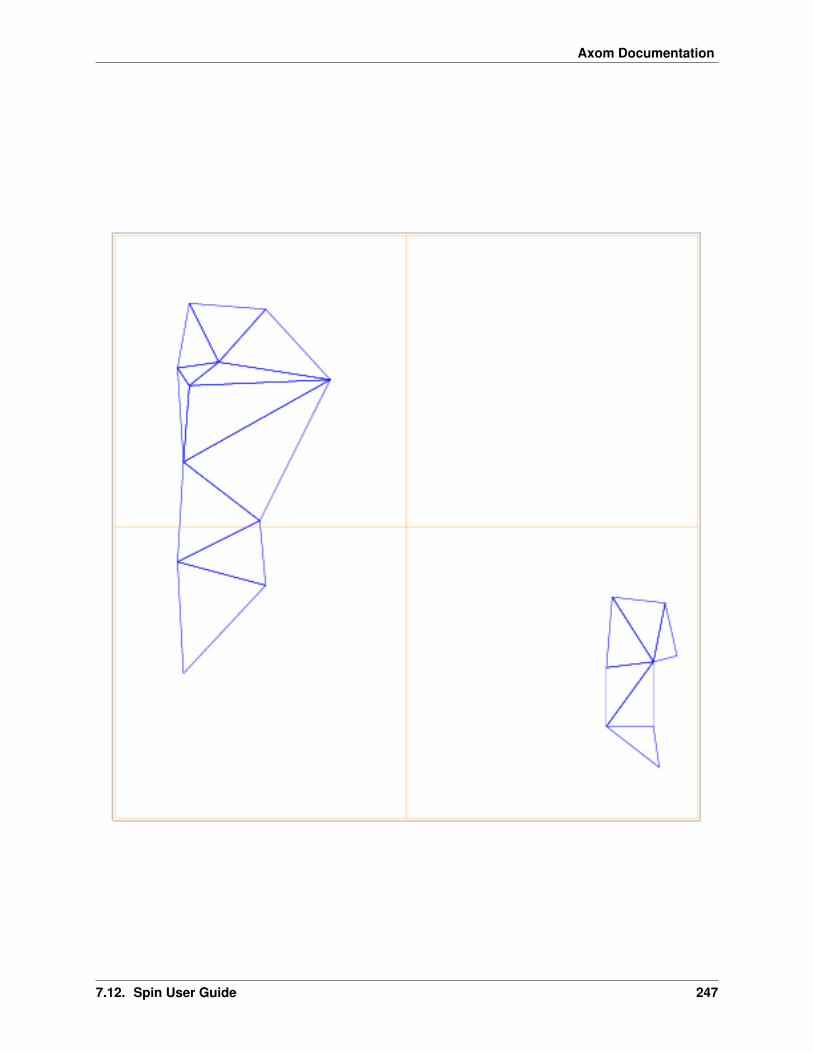
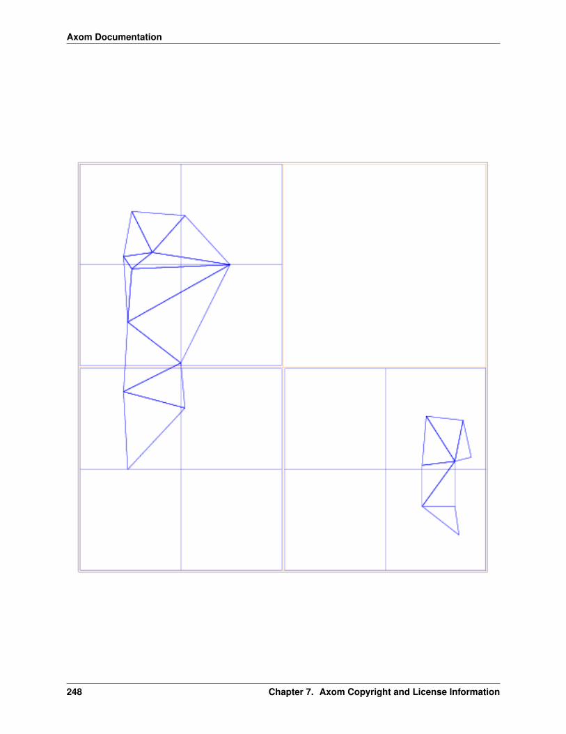
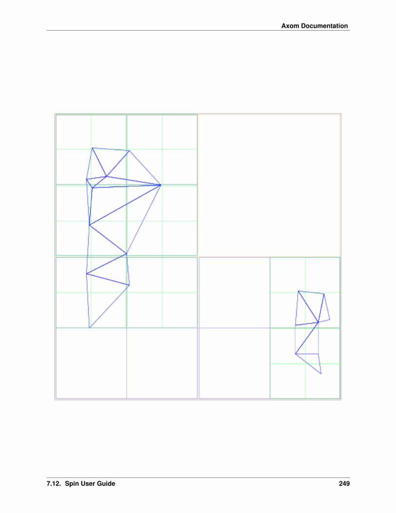
Axom Documentation

#include "axom/spin/SpatialOctree.hpp"

using LeafNodeType = axom::spin::BlockData;

using OctreeType = axom::spin::SpatialOctree<in3D, LeafNodeType>;using OctBlockIndex = OctreeType::BlockIndex;using OctSpacePt = OctreeType::SpacePt;using OctBBox = OctreeType::GeometricBoundingBox;

Then, instantiate the SpatialOctree and locate or refine blocks that contain query points.

OctBBox bb(OctSpacePt(10), OctSpacePt(20));

// Generate a point within the bounding boxdouble alpha = 2. / 3.;OctSpacePt queryPt = OctSpacePt::lerp(bb.getMin(), bb.getMax(), alpha);

// Instantiate the OctreeOctreeType octree(bb);

// Find the block containing the query pointOctBlockIndex leafBlock = octree.findLeafBlock(queryPt);// and the bounding box of the block.OctBBox leafBB = octree.blockBoundingBox(leafBlock);

for(int i = 0; i < octree.maxInternalLevel(); ++i)// SpatialOctree allows a code to refine (subdivide) a blockoctree.refineLeaf(leafBlock);// and locate the (new) child block containing the query point.leafBlock = octree.findLeafBlock(queryPt);

Unlike the BVHTree class, the SpatialOctree is intended as a building block for further specialization. Pleasesee the quest::InOutOctree as an example of this.

Some ancillary classes used in the implementation of SpatialOctree include BlockData, which ties datato a block; Brood, used to construct and organize sibling blocks; OctreeBase, implementing non-geometricoperations such as refinement and identification of parent or child nodes; and SparseOctreeLevel andDenseOctreeLevel, which hold the blocks at any one level of the SpatialOctree. Of these, library userswill probably be most interested in providing a custom implementation of BlockData to hold algorithm data asso-ciated with a box within an octree. See the quest::InOutOctree class for an example of this.

7.13 Developer Guide

This guide describes important aspects of software development processes used by the Axom project. It does notcontain information about building the code or coding guidelines. Please see the note below.

This development guide is intended for all team members and contributors. It is especially helpful for individuals whoare less familiar with the project and wish to understand how the team works. We attempt to employ simple practicesthat are easy to understand and follow and which improve our software without being overly burdensome. We believethat when everyone on our team follows similar practices, the likelihood that our software will be high quality (i.e.,robust, correct, easy to use, etc.) is improved. Everyone who contributes to Axom should be aware of and follow theseguidelines.


Axom Documentation

We also believe that the benefits of uniformity and rigor are best balanced with allowances for individual preferences,which may work better in certain situations. Therefore, we do not view these processes as fixed for all time. Theyshould evolve with project needs and be improved when it makes sense. Changes should be agreed to by team membersafter assessing their merits using our collective professional judgment. When changes are made, this guide should beupdated accordingly.

Note: This document does not describe how to configure and build the Axom code, or discuss Axom coding guide-lines. For information on those topics please refer to the following documents: Axom Quickstart Guide, Axom CodingGuide.

Contents:

7.13.1 Development Process Summary

This section provides a high-level overview of key Axom software development topics and includes links to moredetailed discussion.

Software Development Cycles

The Axom team uses a sprint-based development process. We collect and track issues (bugs, feature requests, tasks,etc.) using Github and define a set of development tasks (i.e., issues) to complete for each sprint. While the teammeets to discuss issues and plan which ones will be worked in each sprint, developers of individual Axom componentsmay plan and schedule work in any way that works for them as long as this is coordinated with other team efforts.Work performed in each sprint work period is tracked as a single unified sprint encompassing activities for the entireproject.

Software Releases and Version Numbers

Typically, Axom releases are done when it makes sense to make new features or other changes available to users. Arelease may coincide with the completion of a sprint cycle or it may not.

See Release Process for a description of the Axom release process.

The Axom team follows the semantic versioning scheme for assigning release numbers. Semantic versioning conveysspecific meaning about the code and modifications from version to version by the way version numbers are constructed.

See Semantic Versioning for a description of semantic versioning.

Branch Development

The Axom project has a Github project space and the team follows the Gitflow branching model for softwaredevelopment and reviews. Gitflow is a common workflow centered around software releases. It makes clear whichbranches correspond to which phases of development and those phases are represented explicitly in the structure ofthe source code repository. As in other branching models, developers develop code locally and push their work to acentral repository.

See Gitflow Branching Model for a detailed description of how we use Gitflow.

7.13. Developer Guide 251

../quickstart_guide/index.html

../coding_guide/index.html


Axom Documentation

Code Reviews and Acceptance

Before any code is merged into one of our main Gitflow branches (i.e., develop or main), it must be adequately tested,documented, and reviewed for acceptance by other team members. The review process is initiated via a pull requeston the Axom Github project.

See Pull Requests and Code Reviews for a description of our review process and how we use pull requests.

Testing and Code Health

Comprehensive software testing processes and use of code health tools (e.g., static analysis, memory checkers, codecoverage) are essential ingredients in the Axom development process.

See Tests and Examples for a description of our software testing process, including continuous integration.

Software Development Tools

In addition to the tools listed above, we use a variety of other tools to help manage and automate our software devel-opment processes. The tool philosophy adopted by the Axom project focuses on three central tenets:

• Employ robust, commonly-used tools and don’t re-invent something that already exists.

• Apply tools in ways that non-experts find easy to use.

• Strive for automation and reproducibility.

The main interaction hub for Axom developers is the Atlassian tool suite on the Livermore Computing CollaborationZone (CZ). These tools can be accessed through the MyLC Portal. Developer-level access to Axom project spaces inthese tools requires membership in the LC group ‘axomdev’. If you are not in this group, and need to be, please sendan email request to ‘[email protected]’.

The main tools we use are listed below. Please navigate the links provided for details about how we use them andhelpful information about getting started with them.

• Confluence. We use the Axom Confluence space for team discussion (e.g., hashing out design ideas), maintain-ing meeting notes, etc.

• Github. We use the Axom Github project to manage our issues and Git repository which contains the Axomsource code, build configurations, scripts, test suites, documentation, etc.

– See Git/Github: Version Control and Branch Development for more information about how we use Gitand Github.

• Gitlab. We use Gitlab for continuous integration to ensure code quality on our LC systems.: Axom Gitlabproject

– See LC GitLab for more information about how we use Gitlab.

• Azure Pipelines. We use Azure Pipelines for continuous integration to ensure every code change passes a levelof quality before being merged.: Azure Pipelines

– See Azure Pipelines for more information about how we use Azire Pipelines.

7.13.2 Continuous Integration

The Axom project uses two CI tools, Azure Pipelines via Github and GitLab CI on the LLNL LC Collaboration Zone(CZ).


https://lc.llnl.gov


https://lc.llnl.gov/confluence/display/ASCT


https://lc.llnl.gov/gitlab/axom/axom


https://azure.microsoft.com/en-us/services/devops/pipelines/

https://azure.microsoft.com/en-us/services/devops/pipelines/

https://docs.gitlab.com/ee/ci/

Axom Documentation

Azure Pipelines

Every Pull Request created on Github is automatically run through a series of CI jobs to ensure that the Axom sourcebuilds and passes our unit tests. These configurations mimic the LC compilers and systems as closely as possible viaDocker containers that have our third-party libraries pre-built on them.

Axom’s Github project is also configured to require pull requests to pass checks from our LC GitLab CI (as describedbelow).

LC GitLab

We also maintain a mirror of the Axom project on LLNL’s LC GitLab instance primarily for testing Axom pull requestsagainst the various LC System Types and compilers.

There are two types of GitLab plans. The first is triggered automatically by pull requests on GitHub, while the secondruns nightly and tests Axom’s develop branch against a new build of our third-party library stack.

Our GitLab CI configuration also allows manual runs. To initiate a new run, navigate to the CI/CD page, click on the“Run pipeline” button and select the branch to test.

7.13.3 Release Process

The Axom team decides as a group when the code is ready for a release. Typically, a release is done when we wantto make changes available to users; e.g., when some new functionality is sufficiently complete or we want users to trysomething out and give us feedback early in the development process. A release may also be done when some otherdevelopment goal is reached. This section describes how an Axom releases is done. The process is fairly informal.However, we want to ensure that the software is in a reasonably robust and stable state when a release is done. Wefollow this process to avoid simple oversights and issues that we do not want to pass on to users.

In the Gitflow Branching Model section, we noted that the main branch records the official release history of theproject. Specifically, whenever, the main branch is changed, it is tagged with a new version number. We use a git‘lightweight tag’ for this purpose. Such a tag is essentially a pointer to a specific commit on the main branch.

We finalize preparations for a release on a release branch so that other work may continue on the develop branchwithout interruption.

Note: No significant code development is performed on a release branch. In addition to preparing release notes andother documentation, the only code changes that should be done are bug fixes identified during release preparations

Here are the steps to follow for an Axom release.

1: Start Release Candidate Branch

Create a release candidate branch off of the develop branch to initiate a release. The name of a release branch mustcontain the associated release version number. Typically, we use a name like v0.5.0-rc (i.e., version 0.5.0 releasecandidate). See Semantic Versioning for a description of how version numbers are chosen.

2: Issue a Pull Request

Create a pull request to merge the release candidate branch into main so that release changes can be reviewed. Suchchanges include:



https://lc.llnl.gov/gitlab/axom/axom/-/pipelines

Axom Documentation

1. Update the version information (major, minor, and patch version numbers) at the top of the axom/src/cmake/AxomVersion.cmake file and in the axom/RELEASE file.

2. Update the release notes in axom/RELEASE-NOTES.md by adding the release version number and releasedate in the heading, as well as, the corresponding link to the version on Github.

3. Test the code by running it through all continuous integration tests and builds. This will ensure that all buildconfigurations are working properly and all tests pass.

4. Fix any issues discovered during final release testing if code changes are reasonably small and re-run appropriatetests to ensure issues are resolved. If a major bug is discovered, and it requires significant code modifications tofix, do not fix it on the release branch. Create a new Github issue for it and note it in the known bugs sectionof the release notes.

5. Make sure all documentation (source code, user guides, etc.) is updated and reviewed. This should not be asubstantial undertaking as most of this should have been done during the regular development cycle.

6. Proofread the release notes for completeness and clarity and address any shortcomings. Again, this should nottake much time as release notes should be updated during the regular development cycle. See Release Notes forinformation about release notes.

3: Merge Release Candidate

Merge the release candidate branch into the main branch once it is ready and approved. At this point, the releasecandidate branch can be deleted.

4: Draft a Github Release

Draft a new Release on Github

1. Enter the desired tag version, e.g., v0.5.0

2. Select main as the target branch to tag a release.

3. Enter a Release title. We typically use titles of the following form Axom-v0.3.1

4. Copy and paste the information for the release from the axom/RELEASE-NOTES.md into the release descrip-tion (omit any sections if empty).

5. Publish the release. This will create a tag at the tip of the main branch and add corresponding entry in theReleases section

Note: Github will add a corresponding tarball and zip archives consisting of the source files for each release. However,these files do not include any submodules. Consequently, a tarball that includes all of the submodules is generatedmanually in a seperate step.

5: Make a Release Tarball

• Checkout the main branch locally and run axom/scripts/make_release_tarball.sh--with-data This will generate a two tarballs of the form Axom-v0.3.1.tar.gz and AxomData-v0.3.1.tar.gz each consistsing of the axom source and data respectively.

• Upload the tarballs for the corresponding release, by going to the Github Releases section and Edit the releasecreated earlier.

• Attach the tarball to the release.


https://github.com/LLNL/axom/issues/new

https://github.com/LLNL/axom/releases/new

https://github.com/LLNL/axom/releases

https://github.com/LLNL/axom/releases

Axom Documentation

• Add a note at the top of the release description that indicates which tarball consists of all the submodules, e.g.,“Please download the Axom-v0.3.1.tar.gz tarball below, which includes all of the Axom submodules as well”

• Update the release.

6: Merge Main to Develop

Create a pull request to merge main into develop. When approved, merge it.

7.13.4 Release Notes

Axom release notes are maintained in a single file axom/RELEASE-NOTES.md. The release notes for the latestversion are at the top of the file. Notes for previous releases appear after that in descending version number order.

For each version, the release notes must contain the following information:

• Axom version number and date of release

• One or two sentence overview of release, including any major changes.

• Release note items should be broken out into the following sections:

– Added: Descriptions of new features

– Removed: Notable removed functionality

– Deprecated: Deprecated features that will be removed in a future release

– Changed: Enhancements or other changes to existing functionality

– Fixed: Major bug fixes

– Known bugs: Existing issues that are important for users to know about

Note: Release notes for each Axom version should explain what changed in that version of the software – and nothingelse!!

Release notes are an important way to communicate software changes to users (functionality enhancements, newfeatures, bug fixes, etc.). Arguably, they are the simplest and easiest way to do so. Each change listed in the releasenotes should contain a clear, concise statement of the change. Items should be ordered based on the impact to users(higher impact - first, lower impact last).

Note: When writing release notes, think about what users need to know and what is of value to them.

Release notes should summarize new developments and provide enough detail for users to get a clear sense of what’snew. They should be brief – don’t make them overly verbose or detailed. Provide enough description for users tounderstand a change, but no more than necessary. In other words, release notes summarize major closed issues in ahuman-readable narrative. Direct users to other documentation (user guides, software documentation, example codes)for details and additional information.

Note: Release notes should be updated as work is completed and reviewed along with other documentation in a pullrequest. This is much easier than attempting to compile release notes before a release by looking at commit logs, etc.Preparing release notes as part of the release process should take no more than one hour.


Axom Documentation

Lastly, release notes provide an easy-to-find retrospective record of progress for users and other stakeholders. Theyare useful for developers and for project reporting and reviews.

7.13.5 Semantic Versioning

The Axom team uses the semantic versioning scheme for assigning release numbers. Semantic versioning is a method-ology for assigning version numbers to software releases in a way that conveys specific meaning about the code andmodifications from version to version. See Semantic Versioning for a more detailed description.

Version Numbers and Meaning

Semantic versioning is based on a three part version number MM.mm.pp:

• MM is the major version number. It is incremented when an incompatible API change is made. That is, theAPI changes in a way that may break code using an earlier release of the software with a smaller major versionnumber. Following Gitflow (above), the major version number may be changed when the develop branch ismerged into the main branch.

• mm is the minor version number. It changes when functionality is added that is backward-compatible. The APImay grow to support new functionality. However, the software will function the same as any earlier release ofthe software with a smaller minor version number when used through the intersection of two APIs. FollowingGitflow (above), the minor version number is always changed when the develop branch is merged into the mainbranch, except possibly when the major version is changed.

• pp is the patch version number. It changes when a bug fix is made that is backward compatible. That is, such abug fix is an internal implementation change that fixes incorrect behavior. Following Gitflow (above), the patchversion number is always changed when a hotfix branch is merged into main, or when develop is merged intomain and the changes only contain bug fixes.

What Does a Change in Version Number Mean?

A key consideration in meaning for these three version numbers is that the software has a public API. Changes tothe API or code functionality are communicated by the way the version number is incremented. Some importantconventions followed when using semantic versioning are:

• Once a version of the software is released, the contents of the release must not change. If the software ismodified, it must be released as a new version.

• A major version number of zero (i.e., 0.mm.pp) is considered initial development where anything may change.The API is not considered stable.

• Version 1.0.0 defines the first stable public API. Version number increments beyond this point depend on howthe public API changes.

• When the software is changed so that any API functionality becomes deprecated, the minor version numbermust be incremented.

• A pre-release version may be denoted by appending a hyphen and a series of dot-separated identifiers after thepatch version. For example, 1.0.1-alpha, 1.0.1-alpha.1, 1.0.2-0.2.5.

• Versions are compared using precedence that is calculated by separating major, minor, patch, and pre-releaseidentifiers in that order. Major, minor, and patch numbers are compared numerically from left to right. Forexample, 1.0.0 < 2.0.0 < 2.1.0 < 2.1.1. When major, minor, and patch numbers are equal, a pre-release versionhas lower precedence. For example, 1.0.0-alpha < 1.0.0.

By following these conventions, it is fairly easy to communicate intent of version changes to users and it should bestraightforward for users to manage dependencies on Axom.


http://semver.org

Axom Documentation

7.13.6 Gitflow Branching Model

The Axom team uses the ‘Gitflow’ branch development model, which is summarized in this section. See the AtlassianGitflow Description for more details.

Gitflow is a branching model centered around software releases. It is a simple workflow that makes clear whichbranches correspond to which phases of development and those phases are represented explicitly in the structure of therepository. As in other branching models, developers develop code locally and push their work to a central repository.

Main and Develop Branches

The main and develop branches are the two main branches used in Gitflow. They always exist and the distinctionbetween them is central to the Gitflow model. Other branches are temporary and used to perform specific developmenttasks.

The main branch records the official release history of the project. Each time the main branch is changed, it is taggedwith a new version number. For a description of our versioning scheme, see Semantic Versioning.

The develop branch is used to integrate and test new features and most bug fixes before they are merged into main.

Important: Development never occurs directly on the main or develop branches.

Topic Branches

Topic branches are created off of other branches (usually develop) and are used to develop new features and resolveissues before they propagate to main. Topic branches are temporary, living only as long as they are needed to completea development task.

Each new feature, or other well-defined portion of work, is developed on its own topic branch, with changes beingpushed to the central repository regularly for backup. We typically include a label, such as “feature” or “bugfix”, inthe topic branch name to make it clear what type of work is being done on the branch. See Topic Branch Developmentfor a description of common Git mechanics when doing topic branch development.

When a feature is complete, a pull request is submitted for review by other team members. When all issues arising ina review have been addressed and reviewers have approved the pull request, the feature branch is merged into develop.See Pull Requests and Code Reviews for more information about code reviews and pull request approval.

Important: Feature branches never interact directly with the main branch.

Release Branches

Release branches are another important temporary branch type in Gitflow: When the team has decided that enoughfeatures, bug fixes, etc. have been merged into develop (for example, all items identified for a release have beencompleted), a release branch is created off of develop to finalize the release. Creating a release branch starts the nextrelease cycle on develop. At that point, new work can start on feature branches for the next release. Only changesrequired to complete the release are added to a release branch. When a release branch is ready, it is merged into mainand main is tagged with a new version number. Finally, main is merged back into develop since it may have changedsince the release was initiated.

The basic mechanics for generating a new release of the main branch for the Axom project are described in ReleaseProcess.


https://www.atlassian.com/git/tutorials/comparing-workflows/gitflow-workflow

https://www.atlassian.com/git/tutorials/comparing-workflows/gitflow-workflow

Axom Documentation

Important: No new features are added to a release branch. Only bug fixes, documentation, and other release-oriented changes go into a release branch.

Hotfix Branches

The last important temporary branch type in Gitflow is a hotfix branch. Sometimes, there is a need to resolve an issuein a released version on the main branch. When the fix is complete, it is reviewed using a pull request and then mergedinto both main and develop when approved. At this point, main is tagged with a new version number. A dedicated lineof development for a bug fix, using a hotfix branch, allows the team to quickly address issues without disrupting otherparts of the workflow.

Important: Hotfix branches are the only branches created off of main.

Gitflow Illustrated

The figure below shows how branches interact in Gitflow.

Fig. 7.34: This figure shows typical interactions between branches in the Gitflow workflow. Here, main was mergedinto develop after tagging version v0.1. A fix was needed and so a hotfix branch was created. When the fix wascompleted, it was merged into main and develop. Main was tagged with version v0.2. Also, work was performed ontwo feature branches. When one feature branch was done, it was merged into develop. Then, a release branch wascreated and it was merged into main when the release was finalized. Finally, main was tagged with version v1.0.


Axom Documentation

7.13.7 Git/Github: Version Control and Branch Development

This section provides information about getting started with Git and Github and describes some mechanics of topicbranch development on the Axom project. For most project work, we interact with our Git repository via our Githubproject.

If you are new to the Git or want to brush up on its features, there are several good sources of information available onthe web:

• Atlassian Git Tutorial has a lot of useful stuff.

• The Git Docs is a complete reference for Git commands and options. It also provides some cheat sheets you candownload.

• Learn Git Branching is nice for visual, hands-on learners.

• The e-book Pro Git, by Scott Chacon is an excellent overview guide to using Git effectively.

SSH Keys

If you have not used Github before, you should start by creating and adding your SSH keys to Github. Github providesa good tutorial here. Performing these two simple steps will make it easier for you to interact with our Git repositorywithout having to repeatedly enter login credentials.

Cloning the Repo

All development work on Axom is performed in a local workspace copy of the Git repository. To make a localworkspace copy, you clone the repo into a directory that you will work in. This is done by typing:

$ git clone --recursive [email protected]:LLNL/axom.git

Note: You don’t need to remember the URL for the Axom repo above. It can be found by going to the Axom repo onour Github project and clicking on the ‘Clone or download’ button on the upper right hand corner above the source.

The ‘–recursive’ argument above is needed to pull in all Git submodules that we use in the project. In particular, youwill need the BLT build system, which is a Git sub-module in Axom, in your local copy of the repo. In case you forgetto pass the ‘–recursive’ argument to the ‘git clone’ command, you can type the following commands after cloning:

$ cd axom$ git submodule init$ git submodule update

Either way, the end result is the same and you are good to go.

Git Environment Support

After cloning, we recommend that you run the development setup script we provide in the top-level Axom directoryto ensure that your Git environment is configured properly; i.e.,:

$ cd axom$ ./scripts/setup-for-development.sh




https://www.atlassian.com/git/

https://git-scm.com/docs/

http://learngitbranching.js.org/

https://git-scm.com/book/en/v2

https://help.github.com/en/enterprise/2.18/user/github/authenticating-to-github/adding-a-new-ssh-key-to-your-github-account

Axom Documentation

This script sets up several things we find useful, such as Git editor, aliases, client-side hooks, useful tips, etc.

You can also define your own aliases for common git commands to simplify your workflow. For example, the followingsets up an alias for unstaging files:

$ git config alias.unstage 'reset HEAD--'

Then, the alias can be used as a regular Git command as illustrated below:

$ git unstage <file>

Moreover, you may want to tap in to some of your shell’s features to enhance your Git experience. Chief among themost notable and widely used features are:

1. Git Completion, which allows tab-completion of Git commands and branch names.

2. Prompt Customization, which allows modifying your prompt to indicate the current branch name, whether thereare local changes, etc.

Git ships with contributed plugins for popular shells. Examples illustrating how to use these plugins in bash andtcsh/csh are given below.

Setting up your Bash Environment

If you are in Bash, you can set your environment as follows:

1. Get the git-prompt.sh and auto-completion scripts from github

$ wget https://raw.githubusercontent.com/git/git/master/contrib/completion/git-→˓prompt.sh$ wget https://raw.githubusercontent.com/git/git/master/contrib/completion/git-→˓completion.bash

2. Optionally, you may want to move the files to another location. Nominaly, folks put those as hidden files in theirhome directory

$ mv git-prompt.sh $HOME/.git-prompt.sh$ mv git-completion.bash $HOME/.git-completion.bash

3. Add the following to your .bashrc

source ~/.git-prompt.shsource ~/.git-completion.bashexport GIT_PS1_SHOWDIRTYSTATE=1export GIT_PS1_SHOWSTASHSTATE=1export GIT_PS1_SHOWUNTRACKEDFILES=1

## Set your PS1 variablereset=$(tput sgr0)bold=$(tput bold)export PS1='[\w] \[$bold\]$(__git_ps1 " (%s)")\[$reset\]\n\[$bold\]\u@\h\[→˓$reset\] > '

Setting up your tcsh/csh Environment

Likewise, if you are using tcsh/csh, you can do the following:


Axom Documentation

1. Get the auto-completion scripts from github. Note, git-completion.tcsh makes calls to git-completion.bash, soyou need to have both

$ wget https://raw.githubusercontent.com/git/git/master/contrib/completion/git-→˓completion.tcsh$ wget https://raw.githubusercontent.com/git/git/master/contrib/completion/git-→˓completion.bash

2. Optionally, you may want to move the files to another location. Nominally, folks put those as hidden files intheir home directory

$ mv git-completion.tcsh $HOME/.git-completion.tcsh$ mv git-completion.bash $HOME/.git-completion.bash

3. Add the following to your .tcshrc or .cshrc

source ~/.git-completion.tcsh

## Add alias to get the branchalias __git_current_branch 'git rev-parse --abbrev-ref HEAD >& /dev/null && echo "→˓`git rev-parse --abbrev-ref HEAD`"'

## Set your prompt variable for example:alias precmd 'set prompt="%n@%m[%c2]`__git_current_branch` "'

Topic Branch Development

It is worth re-emphasizing a fundamental principle of the Gitflow development model that we described in GitflowBranching Model.

Important: We never work directly on the develop or main branches. All development occurs on topicbranches.

When we refer to a topic branch, it could be a feature branch, a bugfix branch, etc. The basic workflow for performingdevelopment on a topic branch is:

1. Create a topic branch off the develop branch and push the new branch to Github.

2. Make changes and commit them to your branch in your local copy of the repository. Remember to push changesto the Github repo regularly for backup and so you can easily recover earlier versions of your work if you needto do so.

3. If you are working on your topic branch for a while, it is a good idea to keep your topic branch current with thedevelop branch by merging develop into your topic branch regularly. This will simplify the process of mergingyour work into the develop branch when you are ready.

4. When your work is complete (including required testing, documentation, etc.), create a pull request so others onthe team can review your work. See Pull Requests and Code Reviews.

Here are some details about each of these steps.

Step 1 – Create a topic branch

Most development occurs on a topic branch created off the develop branch. Occasions where a branch iscreated from another branch, such as a ‘hotfix’ branch created off main, are described in Gitflow Branching


Axom Documentation

Model. To create a branch in Git, provide the -b option to the git checkout command, followed bythe name of your topic branch. A topic branch name should include your username (i.e., login id) and abrief description indicating the purpose of the branch. Typically, we label such branches using “feature”,“bugfix”, etc. to make it clear what type of work is being performed on a branch. For example,:

$ git checkout -b feature/<userid>/my-cool-new-feature$ git push -u

You can also attach a Github issue number to the branch name if the work you will do on the branch isrelated to a issue. Then, Github will associate the issue with the commit when you merge your branch tothe develop branch. For example,:

$ git checkout -b bugfix/<userid>/issue-atk-<issue #>$ git push -u

Alternatively, if your branch addresses multiple issues, you should add the appropriate issue numbers(e.g., #374) to the messages in your commits that address them.

In each of these examples, the ‘git push -u’ command pushes the branch to the Github server and it willappear in the list of branches you and other developers can see there.

Step 2 – Do development work

After you’ve created a topic branch and pushed it to Github, perform your development work on it; i.e.,edit files, add files, etc. Common commands you will use are:

$ git add <file>$ git commit$ git push

The ‘add’ command adds a file (or files) to be staged for a commit operation. The ‘commit’ commandmoves your staged changes to your local copy of the repository. The ‘push’ command pushes thesechanges to the topic branch in the Git repo. To push your work, you could also do:

$ git push origin

This is equivalent to ‘git push’ if you specified the ‘-u’ option when you originally pushed your topicbranch when you created it.

Important: You may perform several local commits before you push your work to the Github repo.Generally, it is a good idea to limit the amount of modifications contained in any one commit. By restrict-ing individual commits to a reasonable size that contain closely related work, it is easier to refer back tospecific changes you make when the need arises (as it inevitably will!). For example, if you regularly runyour code through a formatting tool (we use clang-format on the Axom project), it is preferable to commitother content changes first and then commit formatting changes in a separate commit. That way, you candistinguish substance from cosmetic changes easily in the Git history.

Recall the Git environment setup script we recommended that you run after cloning the repo in the Cloningthe Repo section above. One of the Git pre-commit hooks that the script sets up applies formatting con-straints on the commit message you provide when you execute the ‘commit’ command. The constraintsare recommended Git practices that help make it easier to use various tools with the Git version controlsystem. Specifically:

• Commit message subject line is at most 50 characters


Axom Documentation

• Subject line and body of commit message are separated by a blank line

• Main body of commit message is wrapped to 78 characters

Step 3 – Keep current with develop

If you will be working on your topic branch for a while, it is a good idea to merge changes (made byother developers) from the develop branch to your topic branch regularly. This will help avoid gettingtoo far out of sync with the branch into which your work will be merged eventually. Otherwise, you mayhave many conflicts to resolve when you are ready to merge your topic branch into develop and the mergecould be difficult.

Before you begin the merge, make sure all outstanding changes to your topic branch are committed. Then,make sure your local repo is up-to-date with the develop branch by checking it out and pulling in the latestchanges; i.e.,:

$ git checkout develop$ git pull

Next, checkout your topic branch and merge changes in from the develop branch, and check for conflicts:

$ git checkout <your topic branch>$ git merge develop

The ‘merge’ command will tell you whether there are conflicts and which files have them. Hopefully, youwill not see any conflicts and you can continue working on your topic branch. If there are conflicts, youmust resolve them before you will be able to merge your topic branch to develop. So, you may as wellresolve them right away. You can resolve them by editing the conflicting files and committing the changes.Merge conflicts appear in a file surrounded by lines with special characters on them. For example, if youopen a conflicted file in an editor, you may see:

<<<<<<< HEAD// lines of code, etc...=======// more lines of code, etc...>>>>>>> develop

The section above the ‘=======’ line are the file contents in the current branch head (your topic branch).The lines below are the contents of the develop branch that conflict with yours. To resolve the conflict,choose the correct version of contents you want and delete the other lines.

Alternatively, you can use a tool to help resolve your conflicts. The ‘git mergetool’ command helps yourun a merge tool. One such tool is called “meld”, which is very powerful and intuitive. Diff tools like“tkdiff” are also helpful for resolving merge conflicts.

Important: Git will not let you commit a file with merge conflicts. After you resolve merge conflictsin a file, you must stage the file for commit (i.e., git add <filename>), commit it (i.e., ‘git commit), andpush it to the Github repo (i.e., git push) before you can merge.

Step 4 – Create a pull request

When your work is complete, and you are ready to merge your topic branch to the develop branch, youmust initiate a pull request in Github. Go into the Axom Github project, select your branch, and click


Axom Documentation

Create pull request in the left column. Make sure you select the correct destination branch. The defaultdestination branch in our project is set up to be the develop branch. So, in most cases, you won’t have todo anything special.

You must also select appropriate team members to review changes. Our Github project is set up to requireat least one other developer to approve the pull request before a merge.

Important: You cannot approve your own pull request.

When your pull request is approved (see Code Review Checklist for more information), you merge yourtopic branch to the develop branch by clicking the “merge” button in Github. If there are no mergeconflicts, the merge will proceed and you are done. If there are conflicts, Github will indicate this andwill not let you merge until all conflicts are resolved.

The preferred way to resolve conflicts at this point is to go into your topic branch and do the following:

$ git fetch origin$ git merge origin

The ‘fetch’ command pulls changes from the remote branch into your local branch. Running the ‘merge’command will show which files have conflicts. Fix the conflicts as described in Step 3 – Keep current withdevelop. After all conflicts are resolved, run the ‘commit’ and ‘push’ commands as usual:

$ git commit$ git push

Lastly, complete the merge in Github by clicking the merge button.

Important: To keep things tidy, please delete your topic branch in Github after it is merged if youno longer need it for further development. Github provides an option to automatically delete thesource branch of a merge after the merge is complete. Alternatively, you can click on the Githubbranches tab and manually delete the branch.

Checking Out an Existing Branch

When working on multiple branches, or working on one with someone else on the team, you will need to checkout aspecific branch. Any existing branch can be checked out from the Git repository. Here are some useful commands:

$ git fetch$ git branch -a$ git checkout <branch name>

The ‘fetch’ command retrieves new work committed by others on branches you may have checked out, but withoutmerging those changes into your local copies of those branches. You will need to merge branches if you want changesfrom one branch to be moved into another. The ‘branch’ command lists all available remote branches. The ‘checkout’command checks out the specified branch into your local working space.

Note: You do not give the ‘-b’ option when checking out an existing branch. This option is only used whencreating a new branch.

Here is a concrete example:


Axom Documentation

$ git branch -a | grep homerremotes/origin/feature/homer/pick-up-bart

$ git checkout feature/homer/pick-up-bartBranch feature/homer/pick-up-bart set up to track remote branch feature/homer/pick-

→˓up-bartSwitched to a new branch 'feature/homer/pick-up-bart'

7.13.8 Pull Requests and Code Reviews

Before any code is merged into the develop or main branches, it must be tested, documented, reviewed, and accepted.Creating a pull request on the Axom Github project to merge a branch into develop or main initiates the test andreview processes. All required build configurations and tests must pass for a pull request to be approved. Also, newtests (unit, integration, etc.) must be created that exercise any new functionality that is introduced. This will beassessed by reviewers of each pull request. See Step 4 – Create a pull request for details about creating pull requests.

Code changes in a pull request must be accepted by at least one member of the Axom development team other thanthe originator of the pull request. It is recommended that several team members review pull requests, especiallywhen changes affect APIs, dependencies (within Axom and external), etc. Pull request reviewers can be selected onGithub when the pull request is created. Changes reviewed by the team are accepted, rejected, or commented onfor improvement; e.g., issues to be addressed, suggested changes, etc. Pull requests can be updated with additionalchanges and commits as needed. When a pull request is approved, it can be merged. If the merged branch is no longerneeded for development, it should be deleted.

In addition to successful compilation and test passing, changes to the develop and main branches should be scrutinizedin other ways and using other code health tools we use. See Git/Github: Version Control and Branch Development formore information about using our continuous integration tools.

Pull Request Summary

To recap, here is a summary of steps in a pull request:

1. When code is ready to be considered for acceptance, create a pull request on the Axom Github project. Identifythe appropriate reviewers and add them to the pull request.

2. Code must build successfully and all relevant tests must pass, including new tests required for new functionality.

3. All issues (build failures, test failures, reviewer requests) must be addressed before a pull request is accepted.

4. Pull requests must be approved by at least one member of development team other than the pull request origi-nator.

5. When a pull request is approved it may be merged. If the merged branch is no longer needed, it should bedeleted. This can be done when merging with Github.

Code Review Checklist

Beyond build and test correctness, we also want to ensure that code follows common conventions before acceptance.The following list is a high-level summary of the types of concerns we want to identify during pull request reviewsand resolve before a pull request is merged. Please see the Axom Coding Guide for details on items in this list.

1. A new file or directory must be placed in its proper location; e.g., in the same directory with existing filessupporting related functionality.

2. File contents must be organized clearly and structure must be consistent with conventions.

3. Namespace and other scoping conventions must be followed.



Axom Documentation

4. Names (files, types, methods, variables, etc.) must be clear, easily understood by others, and consistent withusage in other parts of the code. Terminology must be constrained; i.e., don’t introduce a new term for somethingthat already exists and don’t use the same term for different concepts.

5. Documentation must be clear and follow conventions. Minimal, but adequate, documentation is preferred.

6. Implementations must be correct, robust, portable, and understandable to other developers.

7. Adequate tests (unit and performance) tests must be added for new functionality.

7.13.9 Component Structure

This section describes the structure of directories, files, and their contents for an Axom component. This section shouldbe used as a guide to identify tasks to be done when adding a new software component to Axom. These include:

• Creating the appropriate directory structure

• Modifying and adding CMake files and variables

• Generating C and Fortran interfaces

• Writing documentation

• Writing tests

Note: The discussion here does not contain coding guidelines. Please see Axom Coding Guide for that information.

Component Directory Structure

In the axom/src/axom directory, you will find a subdirectory for each Axom component. For example:

$ cd axom/src/axom$ ls -1CMakeLists.txtcoreinletlumberjack...

All files for each component are contained in subdirectories in the component directory.

To illustrate, consider the sidre component directory:

$ cd axom/src/axom/sidre$ ls -1 -FCMakeLists.txtcore/docs/examples/tests/

Note that, besides directories, the top-level component directory contains a few files:

• CMakeLists.txt contains CMake information for the component in the Axom build system.

Components are free to organize their header and source files in whatever manner makes sense. For example, in sidre,these core header and source files are in a subdirectory called core. As is common practice for C++ libraries, associatedheader and source files are co-located in the same directories.



Axom Documentation

The docs directory contains the component documentation. Subdirectories in the docs directory are named for eachtype of documentation. The directories doxygen and sphinx are required. Each Axom component uses Doxygenfor source code documentation and Sphinx for user documentation. Other documentation directories can be usedas needed. For example, sidre also contains documentation directories dot for dot-generated figures, and design fordesign documents.

The interface directory contains interface files for use by languages other than C++. To make it easy for applicationswritten in C and Fortran, for example, to use Axom directly in their native languages, Axom components provide APIsin these languages. For information about how we generate these APIs, see C and Fortran Interfaces.

A test directory is required for each component which contains a comprehensive set of unit tests. See Tests andExamples for information about writing tests and inserting them into our testing framework.

An examples directory is optional, but recommended. It contains simple code examples illustrating component usage.

Important: For consistency, these subdirectory names within the top-level component directory should be the samefor each Axom component.

CMake Files and Variables

To properly configure and compile code for a component, and generate consistent make targets, existing CMake filesand variables need to be modified in addition to adding CMake files for the new component. In this section, wedescribe the sort of changes and additions that are required. For additional details about our CMake and BLT usage,please look in files in existing Axom components.

Add CMake macro definitions

The top-level CMake directory axom/src/cmake contains a file called AxomConfig.cmake that defines macro con-stants for enabling Axom components and setting third-party library (TPL) dependencies that are used to enforceconsistency for conditionally-compiled code. When a new component or dependency is added, that file must be mod-ified by:

1. Adding the name of the component to the COMPS variable

2. Adding new TPL dependency to the TPL_DEPS variable

The CMake variables are used to generate macro constants in the Axom configuration header file. For each newCMake variable added, an associated #cmakedefine definition must be added to the config.hpp.in file in theaxom/src/include directory.

Modify top-level CMakeLists.txt file

When adding a new Axom component, the file axom/src/components/CMakeLists.txt must be modifiedto hook the component into the CMake build configuration system. Specifically:

1. Add option to enable component. For example,:

axom_add_component(COMPONENT_NAME sidre DEFAULT_STATE $AXOM_ENABLE_ALL_→˓COMPONENTS)

2. Add component dependency target by adding component name to the axom_components variable.


Axom Documentation

Add component CMakeLists.txt files

There are several CMakeLists.txt files that must be added in various component directories. We try to maintainconsistent organization and usage across all Axom components to avoid confusion. To illustrate, we describe the keycontents of the CMakeLists.txt files in the sidre Axom component. See those files or those in other components formore details.

Top-level component directory

The top-level component directory contains a CMakeLists.txt, e.g., axom/src/components/sidre/CMakeLists.txt, which contains the following items:

1. A CMake macro call that checks for any of the required components and/or third-party dependencies and errorsout with a helpful message, e.g.,:

axom_component_requires(NAME SidreCOMPONENTS SLICTPLS Conduit )

Note: These dependencies should be limited to the requirements of this singular component. Do not list inher-ited dependencies unless they are used directly in this component. Instead ensure that the upstream componenthas the correct requirements listed.

Note: Optional dependencies should not be listed here. Instead toggle their behaviors via CMake logic byadding defines, source files, and dependencies.

2. Subdirectories additions with guards as needed; e.g.,:

add_subdirectory(src)

and:

if (AXOM_ENABLE_TESTS)add_subdirectory(tests)

endif()

3. CMake exports of component targets; e.g.,:

install(EXPORT <component name>-targets DESTINATION lib/cmake)

4. Code formatting and static analysis targets; e.g.,:

axom_add_code_checks(BASE_NAME <component name>)

Note: Each Axom component should use the common clang-format configuration file defined for the project atsrc/.clang-format. The file is used to define source code formatting options that are applied when the clang-format tool is run on the code.


Axom Documentation

Component src directory

The CMakeLists.txt file in the component src directory defines:

1. A variable for component header files named <component name>_headers

2. A variable for component source files named <component name>_sources

3. A variable for component dependencies named <component name>_depends

For example, these variables for the sidre component are sidre_headers, sidre_sources, andsidre_depends.

Note: It is important to account for all conditional inclusion of items in these CMake variable names. For example, aC interface is generated to support a Fortran API, typically. So if Fortran is not enabled, it is usually not necessary toinclude the C header files in sidre_headers. Similarly, do not include items in the dependency variable if they are notfound.

This file also adds source subdirectories as needed (using the CMake add_subdirectory command), adds thecomponent as a Axom library, and adds target definitions for dependencies. For example, the command to add sidreas a library is:

blt_add_library( NAMEsidre

SOURCES"$sidre_sources""$sidre_fortran_sources"

HEADERS"$sidre_headers"

DEPENDS_ON$sidre_depends

)

All components should follow this format to describe the library information.

Component docs directory

A component docs directory contains a sphinx that has the hand-written user documentation that is built andhosted on the Axom’s ReadTheDocs page. These are included by listing them in the Table of Contents and in theDocumentation section of src/index.rst.

Component tests and examples

The content of component tests and examples directories, including as CMake files are discussed in Tests andExamples.

Filename and CMake Target Conventions for Axom Documentation

The conventions in this section are intended to make it easy to generate a specific piece of documentation for a anAxom component manually. In Axom, we use ‘make’ targets to build documentation. Typing make help will list allavailable targets. When the following conventions are followed, all documentation targets for a component will begrouped together in this listing. Also, it should be clear from each target name what the target is for.

CMake targets for component user guides and source code docs (i.e., Doxygen) are:


https://axom.readthedocs.io/en/develop/index.html

Axom Documentation

<component name>_user_docs

and

<component name>_doxygen_docs

respectively. For example:

sidre_user_docs (sidre component user guide)sidre_doxygen_docs (sidre Doxygen source code docs)

C and Fortran Interfaces

Typically, we use the Shroud tool to generate C and Fortran APIs from our C++ interface code. Shroud is a pythonscript that generate code from a yaml file that describes C++ types and their interfaces. It was developed for theAxom project and has since been generalized and is supported as a standalone project. To illustrate what is needed togenerate multi-language API code via a make target in the Axom build system, we describe the contents of the sidreAxom component interface directory axom/src/components/sidre/src/interface that must be added:

1. A yaml file, named sidre_shroud.yaml, which contains an annotated description of C++ types and theirinterfaces in sidre C++ files. This file and its contents are generated manually.

2. Header files, such as sidre.h, that can be included in C files. Such a file includes files containing Shroud-generated ‘extern C’ prototypes.

3. Directories to hold the generated files for different languages; e.g., c_fortran for C and Fortran APIs,python for python API, etc.

4. ‘Splicer’ files containing code snippets that get inserted in the generated files.

5. A CMakeLists.txt files that contains information for generating CMake targets for Shroud to generate thedesired interface code. For example:

add_shroud( YAML_INPUT_FILE sidre_shroud.yamlYAML_OUTPUT_DIR yamlC_FORTRAN_OUTPUT_DIR c_fortranPYTHON_OUTPUT_DIR pythonDEPENDS_SOURCE

c_fortran/csidresplicer.c c_fortran/fsidresplicer.fpython/pysidresplicer.c

DEPENDS_BINARY genfsidresplicer.f)

This tells shroud which yaml file to generate code files from, which directories to put generated files in, whichsplicer files to use, etc.

The end result of properly setting up these pieces is a make target called generate_sidre_shroud that can beinvoked to generate sidre API code in other languages Axom supports.

Documentation

Complete documentation for an Axom component consists of several parts described in the following sections. Alluser documentation is accessible on Axom Read The Docs page.


https://github.com/LLNL/shroud

https://axom.readthedocs.io

Axom Documentation

User Documentation

Each Axom component uses Sphinx for user documentation. This documentation is generated by invoking appropriatemake targets in our build system. For example, make sidre_docs builds html files from Sphinx user documenta-tion for the sidre component.

The main goal of good user documentation is to introduce the software to users so that they can quickly understandwhat it does and how to use it. A user guide for an Axom component should enable a new user to get a reasonablesense of the capabilities the component provides and what the API looks like in under 30 minutes. Beyond introductorymaterial, the user guide should also help users understand all major features and ways the software may be used. Hereis a list of tips to help you write good documentation:

1. Try to limit documentation length and complexity. Using figures, diagrams, tables, bulleted lists, etc. can helpimpart useful information more quickly than text alone.

2. Use examples. Good examples can help users grasp concepts quickly and learn to tackle problems easily.

3. Place yourself in the shoes of targeted users. Detailed instructions may be best for some users, but may beonerous for others who can quickly figure things out on their own. Consider providing step-by-step instructionsfor completeness in an appendix, separate chapter, via hyperlink, etc. to avoid clutter in sections where you aretrying to get the main ideas across.

4. Try to anticipate user difficulties. When possible, describe workarounds, caveats, and places where software isimmature to help users set expectations and assumptions about the quality and state of your software.

5. Test your documentation. Follow your own instructions completely. If something is unclear or missing, fix yourdocumentation. Working with a co-worker who is new to your work, or less informed about it, is also a goodway to get feedback and improve your documentation.

6. Make documentation interesting to read. While you are not writing a scintillating novel, you want to engageusers with your documentation enough so that they don’t fall asleep reading it.

7. Quickly incorporate feedback. When a user provides some useful feedback on your documentation, it showsthey care enough to help you improve it to benefit others. Incorporate their suggestions in a timely fashion andask them if you’ve addressed their concerns. Hopefully, this will encourage them to continue to help.

Speaking of good user documentation, the reStructuredText Primer provides enough information to quickly learnenough to start using the markdown language for generating sphinx documentation.

Code Documentation

Each Axom component uses Doxygen for code documentation. This documentation is generated by invoking ap-propriate make targets in our build system. For example, make sidre_doxygen builds html files from Doxygen codedocumentation for the sidre component.

The main goal of code documentation is to provide an easily navigable reference document of your software interfacesand implementations for users who need to understand details of your code.

We have a useful discussion of our Doxygen usage conventions in the Documentation Section of the Axom CodingGuide. The Doxygen Manual contains a lot more details.

Axom’s code documentation is published along with our user documentation.

7.13.10 Tests and Examples

This section describes how to build and organize tests and examples for Axom components. These live in tests andexamples directories within each component top-level directory.


http://www.sphinx-doc.org/en/stable/rest.html

../coding_guide/sec07_documentation.html

../coding_guide/sec07_documentation.html

http://www.doxygen.nl/manual/

https://axom.readthedocs.io/en/develop/doxygen/html

https://axom.readthedocs.io

Axom Documentation

Comprehensive collections of well-designed unit tests and integration tests are important tools for developing qualitysoftware. Good tests help to ensure that software operates as expected as it is being developed and as it is used indifferent ways. To maintain a high level of usefulness, tests must be maintained and developed along with the rest ofproject software. Tests should be expanded and modified as software evolves so that they can always be used to verifythat software functionality is correct.

Unit tests are most effective for designing and modifying individual software units to make sure they continue workproperly. Integration tests help to make sure that various sets of software units work together. Typically, integrationtesting is more complex and subtle than the sum of the independent unit tests of the parts that comprise the integratedsystem. Proving that component X and component Y each work independently doesn’t prove that X and Y are com-patible or that they will work together. Also, defects in individual components may bear no relationship to issues anend user would see.

When developing software, it is important to keep these thoughts in mind and to use tests effectively to meet yourgoals. Exposing issues when designing and refactoring individual software components may be best accomplishedwith unit tests, often run manually as you are adding or modifying code. Detecting broken regressions (e.g., “this usedto work, but something changed and now it doesn’t”) may be best done by frequently running automated integrationtests.

This section describes how to write and manually run tests in Axom.

A Few Guidelines for Writing Tests

Before we describe the mechanics of writing tests in the Axom framework, we describe some test guidelines. The aimof these guidelines is to help ensure that tests are complete, correct, easy to run, and easy to modify as needed whensoftware changes.

• Decompose tests so that each test is independent of the others. For example, a unit test file should test featuresof a single class and not contain tests of other classes.

• Each specific behavior should be specified in one and only one test. For example, all unit tests for a con-tainer class may live in a single test file, but you should verify each container operation (e.g., container cre-ation/destruction, item insertion, item removal, container traversal, etc.) in exactly one test. In particular, if atest covers some behavior, checking that same behavior in another test is unnecessary.

• Limit each test to as few logical assertions as possible. Ideally, each behavior should require one logical as-sertion. However, sometimes it makes sense to have more than one check. For example, a test for an emptycontainer may assert that its ‘empty’ method returns true and also assert that its ‘size’ method returns zero.

• Tests should be independent on the order in which they are run.

• Tests should be independent of the platform (hardware architecture, compiler, etc.) on which they are run.

• Tests should be named clearly and consistently. See Filename and CMake Target Conventions for Axom Testsand Examples for a description of Axom conventions for test names.

Unit Tests

In Axom, we use the Google Test framework for C and C++ unit tests and we use the Fortran Unit Test Framework(FRUIT) for Fortran unit tests.

Organization of tests in either language/framework are similar should follow the principles summarized in the guide-lines above. Each Google Test or FRUIT file is compiled into its own executable that can be run directly or as thebuild target test. Each executable may contain multiple tests. So that running individual tests as needed is not overlyburdensome, such as unit tests for a C++ class, we put all tests for distinct software units in files separate from thosefor other units. Tests within each file should be sized so that too many different behaviors are not executed or verifiedin a single test.


https://github.com/google/googletest

https://sourceforge.net/projects/fortranxunit/


Axom Documentation

See Filename and CMake Target Conventions for Axom Tests and Examples for test file naming and make targetconventions.

Google Test (C++/C Tests)

The contents of a typical Google Test file look like this:

#include "gtest/gtest.h"

#include ... // include Axom headers needed to compiler tests in file

// ...

TEST(<test_case_name>, <test_name_1>)

// Test 1 code here...// EXPECT_EQ(...);

TEST(<test_case_name>, <test_name_2>)

// Test 2 code here...// EXPECT_TRUE(...);

// Etc.

Each unit test is defined by the Google Test TEST() macro which accepts a test case name identifier, such as thename of the C++ class being tested, and a test name, which indicates the functionality being verified by the test. Foreach test, logical assertions are defined using Google Test assertion macros. Failure of expected values will cause thetest to fail, but other tests will continue to run.

Note that the Google Test framework will generate a main() routine for each test file if it is not explicitly provided.However, sometimes it is necessary to provide a main() routine that contains operation to run before or after the unittests in a file; e.g., initialization code or pre-/post-processing operations. A main() routine provided in a test fileshould be placed at the end of the file in which it resides.

Here is an example main() from an Axom test that sets up a slic logger object to be used in tests:

int main(int argc, char * argv[])

int result = 0;

::testing::InitGoogleTest(&argc, argv);

SimpleLogger logger; // create & initialize test logger,// finalized when exiting main scope

::testing::FLAGS_gtest_death_test_style = "threadsafe";result = RUN_ALL_TESTS();

return result;

Note that Google Test is initialized first, followed by initialization of the slic SimpleLogger object. TheRUN_ALL_TESTS() Google Test macro will run all the tests in the file.


Axom Documentation

As another example, consider a set of tests that use MPI. The main() routine will initialize and finalize MPI beforeand after tests are run, respectively:

int main(int argc, char * argv[])

int result = 0;

::testing::InitGoogleTest(&argc, argv);

SimpleLogger logger; // create & initialize test logger,// finalized when exiting main scope

MPI_Init(&argc, &argv);

result = RUN_ALL_TESTS();

MPI_Finalize();

return result;

Note that Google test is initialized before MPI_Init() is called.

Other Google Test features, such as fixtures, may be used as well.

See the Google Test Primer for discussion of Google Test concepts, how to use them, and a listing of available assertionmacros, etc.

FRUIT (Fortran Tests)

Fortran unit tests using the FRUIT framework are similar in structure to the Google Test tests for C and C++ describedabove.

The contents of a typical FRUIT test file look like this:

module <test_case_name>use iso_c_bindinguse fruituse <axom_module_name>implicit none

contains

subroutine test_name_1! Test 1 code here...! call assert_equals(...)end subroutine test_name_1

subroutine test_name_2! Test 2 code here...! call assert_true(...)end subroutine test_name_2

! Etc.

The tests in a FRUIT test file are placed in a Fortran module named for the test case name, such as the name of the C++class whose Fortran interface is being tested. Each unit test is in its own Fortran subroutine named for the test name,


https://github.com/google/googletest/blob/master/googletest/docs/Primer.md

Axom Documentation

which indicates the functionality being verified by the unit test. Within each unit test, logical assertions are definedusing FRUIT methods. Failure of expected values will cause the test to fail, but other tests will continue to run.

Note that each FRUIT test file defines an executable Fortran program. The program is defined at the end of the test fileand is organized as follows:

program fortran_testuse fruituse <axom_component_unit_name>implicit nonelogical ok

! initialize fruitcall init_fruit

! run testscall test_name_1call test_name_2

! compile summary and finalize fruitcall fruit_summarycall fruit_finalize

call is_all_successful(ok)if (.not. ok) thencall exit(1)

endifend program fortran_test

Please refer to the FRUIT documentation for more information.

CMake Files and Variables for Tests

The CMakeLists.txt file in component test directory defines the following items:

1. Variables for test source files as needed. Separate variables should be used for Fortran, C++, etc. For example,gtest_sidre_tests for C++ tests, gtest_sidre_C_tests for C tests, and fruit_sidre_testsfor Fortran tests. Note that we use the Google Test framework for C and C++ tests and Fruit for Fortran tests.

2. An executable and test variable for each test executable to be generated. These variables use theblt_add_executable and axom_add_test macros, respectively, as described above.

Note: Fortran executables and tests should be guarded to prevent generation when Fortran is not enabled.

See Tests and Examples for details about writing tests in Axom.

Examples

Examples for Axom components serve to illustrate more realistic usage of those components. They can also be run astests if that’s appropriate.

The source code for each component test should be contained in the component examples directory if it is containedin one file. If it contains multiple files, these should be placed in a descriptively-named subdirectory of the examplesdirectory.

In addition, each example should be given its own CMake-generated make target.



Axom Documentation

CMake Files and Variables for Examples

The CMakeLists.txt file in each component’s examples directory defines the following items:

1. Variables for example source files and header files as needed Separate variables should be used for Fortran, C++,etc. For example, example_sources for C++, F_example_sources for Fortran.

2. An executable and test variable for each example executable to be generated and each executable to be run asa test. These definitions use the blt_add_executable and axom_add_test macros, respectively. Forexample:

blt_add_executable(NAME <example executable name>SOURCES <example source>OUTPUT_DIR $EXAMPLE_OUTPUT_DIRECTORYDEPENDS_ON <example dependencies>)

and:

axom_add_test(NAME <example executable name>COMMAND <example executable name>)

Fortran executables and tests should be guarded to prevent generation if Fortran is not enabled.

Filename and CMake Target Conventions for Axom Tests and Examples

The conventions in this section are intended to make it easy to tell what is in a given component test or example fileand to make it easy to run desired test or example. In Axom, we use make targets to build and run tests and examples.Typing make help will list all available targets. When the following conventions are followed, all test and exampletargets for a component will be grouped together in this listing. Also, it will be clear from each target name what thetarget is for.

Test file names and make targets

The format of a test file name is:

<component name>_<test name>_<optional language specifier>

Examples:

sidre_buffer.cpp ('Buffer' class C++ unit test)sidre_buffer_C.cpp ('Buffer' class C unit test)sidre_buffer_F.f ('Buffer' class Fortran unit test)

When test files are named like this, it is easy to see what they contain. Additionally, when added to the appropriateCMakeLists.txt file (see src/components/sidre/tests/CmakeLists.txt file for example), theextension ‘_test’ will be added to the make target name so that the test will appear as follows in the make target listingwhen make help is typed:

sidre_buffer_testsidre_buffer_C_testsidre_buffer_F_test

Note: We should also add a target for each component to run all its tests; e.g., ‘make sidre_tests’


Axom Documentation

Example file names and make targets

The format of an example file name is:

<component name>_<example name>_<optional language specifier>_ex

Examples:

sidre_shocktube_ex.cpp ('shocktube' C++ example)sidre_shocktube_F_ex.f ('shocktube' Fortran example)

Running Tests and Examples

Axom examples and tests can be run in different ways. Examples and tests can be run individually by manuallyrunning their executables. Built examples are in the build directory under examples and tests are under tests.

Tests can also be ran as a suite with the build target test from the build directory. For example:

$ make test

This will run all tests and examples and report a summary of passes and failures. Detailed output on individual tests issuppressed.

If a test fails, you can invoke its executable directly to see the detailed output of which checks passed or failed. Thisis especially useful when you are modifying or adding code and need to understand how unit test details are working,for example.

7.13.11 Third-party Libraries

Axom dependencies are grouped into four categories: Git submodules, built-in TPLs in the Axom source tree, system-level TPLs, and other TPL libraries. The following sections describe how to install and update these dependencies forAxom.

• How does one add a new compiler or platform to the mix?

• How does one build a new set of TPLs for a single platform or compiler for testing?

• What is the procedure for changing versions of one or more TPLs?

• How do we keep things straight when using different TPL versions for different branches?

• How to use the scripts for team TPL support vs. local development and experimentation?

• Others?

Updating TPLs

Git submodules

Currently, Axom uses three external packages that appear in the repo as Git submodules. These are the following,including the location of the package in the Axom source tree:

• BLT, which is the CMake-based build system we use. Location: axom/src/cmake/blt.

• Axom Data, which is where we maintain data files used in testing Axom. Location: axom/data.


https://github.com/LLNL/blt.git

https://github.com/LLNL/axom_data.git

Axom Documentation

• Uberenv, which contains Python scripts we use to help automate building third-party dependencies for develop-ment and deployment. Location: axom/scripts/uberenv.

There is no software installation process for these dependencies in the traditional sense. To update one of thesepackages in Axom, simply go into its directory in Axom and check out a new version. If a version is intended to bechanged in the Axom repo, make the version change on a branch and submit a GitHub pull request as you would dofor other software changes. More info on Building and Installing Axom.

Built-in TPLs

Axom several lightweight header-only libraries that we use internally and expose for downstream customers to use ifthey wish.

• CLI11, is a command line parser for C++11 and beyond that provides a rich feature set with a simple andintuitive interface.

• fmt, is an open-source formatting library providing a fast and safe alternative to C stdio and C++ iostreams.

• sol, is a C++ library binding to Lua.

• Sparsehash, contains several hash-map implementations.

Note: Axom patches all built-in TPLs to be under the axom namespace. This is to prevent symbol collisionswith other projects, either our dependencies or downstream customers who wish their own versions. For example,fmt::format("foo") is axom::fmt::format("foo").

They can be found in the directory: src/thirdparty. The basic instructions on how to update a built-in TPL areas follows:

1. Download the new release and override the source that is already there. This can often involve removing filesno-longer needed but most of the current ones are a single header file.

2. Review and apply the existing patch files. More than likely, you will not be able to directly apply the patch butit will give you the general idea on what needs to be applied. For example, the namespace update mentionedabove.

3. Ensure that the build and tests still pass. More info on Tests and Examples.

4. Follow the normal pull request work flow. More info on Pull Requests and Code Reviews.

Local Third-party Library Installation

It is often useful to have a different set of TPLs during the development process. For example, you may want to tryout a new library or version of an existing library.

From the top-level Axom directory, run the following script to build all TPLs for all existing compiler specs on theplatform you are currently on:

$ ./scripts/llnl_scripts/build_tpls.py -d local/install/path

where local/install/path is a directory location where you want the libraries to be installed.

It will output whether the TPL install succeeded and, subsequently, whether an Axom build against the TPL installsucceeded.

Running the script produces new host-config files (i.e., CMake cache files) that you can use to build and test Axomwith the installation, if issues arise. The generated host-config files will be located in the top-level Axom directory


https://github.com/LLNL/uberenv.git

https://github.com/CLIUtils/CLI11

https://github.com/fmtlib/fmt

https://github.com/ThePhD/sol2

https://github.com/sparsehash/sparsehash

Axom Documentation

of your local clone of the repo. If any changes to Axom code are needed to work with the TPL update(s), make thechanges and test them.

Note: You can build a subset of TPLs for a platform, by passing a Spack spec arguments to the build_tpls.pyscript. For example,

--spec [email protected]~cpp14+devtools+mfem+c2c

will build the TPLs for the clang 10.0.0 compiler. Please see the scripts/spack/specs.json file for a list ofcurrently tested specs.

Shared Third-party Library Installation Steps

The following instructions describe how to install local copies of Axom TPLs on Livermore Computing (LC) platformsand recreate our Docker containers with a new set of TPLs. Typically, this process is followed when you want to updateone or more TPLs which Axom depends on. After they are built and the required changes are merged into develop,they will be available for other Axom developers to use during development, in Axom Gitlab CI testing, etc.

1. Working on a local branch. Make a local clone of the Axom repo and create a branch to work on.

2. Changing versions of system packages or other TPLs. To change a version of a system package, whichapplies to an LC platforms or a Docker container image we use for CI testing on GitHub, go into the directoryaxom/scripts/spack/configs. There you will find a sub-directory for each supported LC system type.Each sub-directory has a packages.yaml file which contains an entry for each system level package we relyon. Find the entry for the library you wish to update and change the version number. Do this for each systemyou want to test/change, including configurations in the docker subdirectory.

Note: Alongside each packages.yaml in each system package directory, there is a compilers.yamlfile containing compiler and version information for compilers we use for development and testing. If you wishto test and build with a new compiler or version on a system, modify the appropriate compilers.yaml file.

To change a version of a non-system TPL, go into the axom/scripts/spack/packages directory. Thereyou will find a sub-directory for each TPL Axom uses. Modify the contents of the Spack package filepackage.py in each package sub-directory as needed.

Note: Before continuing, you should test that the installation works on all LC systems with the steps in LocalThird-party Library Installation.

3. Install TPLs on all required LC machines. This step needs to be run on each of the machines named inAxom’s standard host-configs. When you are confident that everything is correct, become the service user atkvia the following command:

$ xsu atk

Note: This command requires special access permissions. If you need them, contact the Axom team.

Run the corresponding command for the system you are on:


Axom Documentation

# blueos$ lalloc 1 -W 120 scripts/llnl/build_tpl.py

# toss3$ srun -N1 --interactive -t 120 scripts/llnl/build_tpl.py

This script will build all third-party libraries for all compilers specs for the machine you are on. These will beinstalled into the shared LC directory /usr/workspace/axom/libs/<SYS_TYPE>/<time date>/<compiler> used by Axom developers. When completed, they will produce new host-config files for eachconfiguration. These host-configs will be at the base of the repository and named in the following pattern:<machine name>-<SYS_TYPE>-<compiler spec>.cmake Give these files to your regular user ac-count and log back in to that account. Copy these new host-config files to the host-configs subdirectoryand commit them to your branch. Make sure all file changes from all previous steps are also committed andpushed upstream.

Note: If this step fails, delete the time date stamped directory that was created. If you forget to do this, it willeventually be deleted by hand in bulk when they are past a certain age and no longer needed.

4. Build new Docker images. We utilize Docker images that have pre-built TPLs in our Github CI checks. To buildthese, go to our GitHub Actions page. Click on “Actions” and then on “Docker TPL build” in the “Workflows”menu. Find the “Run Workflow” drop-down menu, select your branch, and click on the “Run workflow” button.This will launch the build of the docker images.

When the docker image build completes, click on your build and find the “Artifacts” listed at the bottom of thepage. These contain host-configs for building Axom on the docker images. Download them and copy them toAxom’s host-configs/docker subdirectory. Rename them to match the corresponding host-config.

5. Update Azure Pipelines to the new Docker images. To complete the setup of the new docker images, theCompiler_ImageName entries in azure-pipelines.yaml at the top-level directory must be updatedwith the timestamped names of the new images. The new names can be found in the log files from the successfulGitHub action. On the left of the page for the successful action is a “Jobs” menu. Click on each job and thenfind the “Get dockerhub repo name” section of the log. The second line of the section there should be an entryof the form axom/tpls:clang-10_12-18-20_00h-10m. Copy the name beginning with axom/tplsto the appropriate locations in azure-pipelines.yaml. Repeat this with the names from each compilerjob used in the GitHub action.

6. Make sure all changes in your branch are committed and pushed, and create a pull request for a merge to develop.If everything went well, all checks on your Github PR should pass.

7.13.12 Miscellaneous Development Items

This section describes various development tasks that need to be performed at times and which are not covered in othersections.

Web Documentation

Axom web-based documentation is hosted on our Read the Docs project. Multiple versions are visible there, includingthe latest content on the develop branch (latest) and the main branch (main). The documentation that appears isautomatically re-generated each time a change is pushed to a branch in the GitHub repository that is enabled to bedisplayed on the Read the Docs project. If you are modifying Axom documentation, you can enable the branch you areworking on so that you can see what it looks like as you push changes to the branch. If your documentation changesare part of a GitHub pull request, it is a good idea to enable the documentation for that branch and put a link to it inthe pull request summary. This makes it easy for reviewers to check over your changes.


https://github.com/LLNL/axom/actions/workflows/docker_build_tpls.yml

https://readthedocs.org/projects/axom/

Axom Documentation

Note: When you no longer need the documentation of your branch to be visible on Read the Docs (e.g., your pullrequest is merged), please disable that branch on Read the Docs.

Code Health Tools

This section describes how to run code health tools we use.

Code Coverage

Setting up and running code coverage analysis. . .

Static Analysis

Setting up and running static analysis tools. . . .

Memory Checking

Setting up and running memory checking tools. . . .

7.14 Coding Guidelines

These guidelines define code style conventions for the Axom project. Most of the items were taken from the citedreferences, sometimes with modifications and simplifications; see References and Useful Resources.

The guidelines emphasize code readability, correctness, portability, and interoperability. Agreement on coding styleand following common idioms and patterns provides many benefits to a project with multiple developers. A uniform“look and feel” makes it easier to read and understand source code, which increases team productivity and reducesconfusion and coding errors when developers work with code they did not write. Also, guidelines facilitate code re-views by enforcing consistency and focusing developers on common concerns. Some of these guidelines are arbitrary,but all are based on practical experience and widely accepted sound practices. For brevity, most guidelines containlittle detailed explanation or justification.

Each guideline is qualified by one of three auxiliary verbs: “must”, “should”, or “may” (or “must not”, “should not”,“may not”).

• A “must” item is an absolute requirement.

• A “should” item is a strong recommendation.

• A “may” item is a potentially beneficial stylistic suggestion.

How to apply “should” and “may” items often depends on the particular code situation. It is best to use these in waysthat enhance code readability and help reduce user and developer errors.

Important:

• Variations in coding style for different Axom components is permitted. However, coding style within eachAxom component must be consistent.

• Deviations from these guidelines must be agreed upon by the Axom team.

7.14. Coding Guidelines 281

Axom Documentation

• When the team agrees to change the guidelines, this guide must be updated.

Contents:

7.14.1 1 Changing Existing Code

Follow existing code style

1.1 When modifying existing code, the style conventions already in use in each file must be followed unless the scopeof changes makes sense (see next item). This is not intended to stifle personal creativity - mixing style is disruptiveand may cause confusion for users and fellow developers.

1.2 When making stylistic changes to existing code, those changes should extend to a point where the style is consis-tent across a reasonable scope. This may mean that an entire file is changed to prevent multiple conflicting styles.

Only change code from other sources when it makes sense

1.3 The Axom project may contain code pulled in from sources outside Axom. These guidelines apply to codedeveloped within Axom primarily. The decision to modify externally-developed code that we pull into Axom willbe evaluated on a case-by-case basis. Modifying such code to be compliant with these guidelines should typically bedone only if a significant rewrite is undertaken for other reasons.

7.14.2 2 Names

Good names are essential to sound software design. This section contains guidelines for naming files, types, func-tions, class members, variables, etc. The main goal is to use clear and unambiguous names. Also, we want namingconventions for different entities so that, when applied, the role of each is obvious from the form of its name.

Good names are clear and meaningful

2.1 Every name must be meaningful. In particular, its meaning must be clear to other code developers and users, notjust the author of the name.

A substantial benefit of good name selection is that it can greatly reduce the amount of developer debateto define a concept. A good name also tends to reduce the amount of documentation required for others tounderstand it. For example, when the name of a function clearly indicates what it does and the meaningand purpose of each argument is clear from its name, then code comments may be unnecessary. Doc-umentation can be a substantial part of software and requires maintenance. Minimizing the amount ofrequired documentation reduces this burden.

Avoid cryptic names

2.2 Tersely abbreviated or cryptic names should be avoided. However, common acronyms and jargon that are wellunderstood by team members and users may be used.

Use terminology consistently

2.3 Terminology must be used consistently; i.e., for names and concepts in the code and in documentation. Multipleterms should not be used to refer to the same concept and a concept should not be referred to by multiple terms.


Axom Documentation

Using a clear, limited set of terminology in a software project helps maintain the consistency and integrityof the software, and it makes the code easier to understand for developers and users.

2.4 Each name must be consistent with other similar names in the code.

For example, if getter/setter methods follow the convention “getFoo” and “setFoo” respectively, thenadding a new setter method called “putBar” is clearly inconsistent.

Name directories so it’s easy to know what’s in them

2.5 Each directory must be named so that the collective purpose of the files it contains is clear. All directory namesshould follow the same style conventions.

All directory names should use all lower case letters and consist of a single word in most cases. Adirectory name with more than one word should use an ‘underscore’ to separate words.

For example, use:

cool_stuff

not

cool-stuff

Follow file extension conventions

2.6 C++ header and source file extensions must be: *.hpp and *.cpp, respectively.

2.7 C header and source files (e.g., tests, examples, and generated API code) must have extensions *.h and *.c,respectively.

2.8 Fortran source files (e.g., tests and examples, and generated API code) must have the extension *.f or *.F . *.Fmust be used if the preprocessor is needed to compile the source file.

Associated source and header file names should match

2.9 The names of associated header and source files should match, apart from the file extension, to make their associ-ation clear.

For example, the header and source files for a class “Foo” should be named “Foo.hpp” and “Foo.cpp”,respectively.

Also, files that are closely related in other ways, such as a header file containing prototypes for a setof methods that are not class members and a source file containing implementations of those methods,should be named the same or sufficiently similar so that their relationship is clear.

File contents should be clear from file name

2.10 The name of each file must clearly indicate its contents.

For example, the header and source file containing the definition and implementation of a major type,such as a class must include the type name of the type in the file name. For example, the header andimplementation file for a class called “MyClass” should be named “MyClass.hpp” and “MyClass.cpp”,respectively.


Axom Documentation

Files that are not associated with a single type, but which contain closely related functionality or concepts,must be named so that the functionality or concepts are clear from the name. For example, files that defineand implement methods that handle file I/O should be named “FileIO.hpp” and “FileUtils.cpp”, or similar.

File names should not differ only by case

2.11 File names that differ only in letter case must not be used.

Since we must support Windows platforms, which have limited case sensitivity for file names, having fileswith names “MyClass.hpp” and “myclass.hpp”, for example, is not acceptable.

Namespace name format

2.12 All namespaces defined must use all lowercase letters for consistency and to avoid user confusion.

Type name format

2.13 Type names (i.e., classes, structs, typedefs, enums, etc.) must be nouns and should be in mixed case with eachword starting with an upper case letter and all other letters in lower cases.

For example, these are preferred type names:

DataStore, MyCollection, TypeUtils

These type names should not be used:

dataStore, mycollection, TYPEUTILS

2.14 Separating characters, such as underscores, should not be used between words in a type name.

For example, these names are not preferred type names:

Data_store, My_Collection

Note: Exceptions to the guidelines above include cases where types play a similar role to those in common useelsewhere. For example, naming an iterator class “base_iterator” would be acceptable if it is conceptually similar withthe C++ standard library class.

2.15 Suffixes that may be used by compilers for name mangling, or which are used in the C++ standard library, suchas “_t”, must not be used in type names.

Function name format

2.16 Function names must use “camelCase” or “pot_hole” style. camelCase is preferred.

camelCase style: The first word has all lower case letters. If multiple words are used, each word after thefirst starts with an upper case letter and all other letters in the word are lower case. Underscores must notbe used in camelCase names, but numbers may be used.

For example, these are proper camelCase names:

getLength(), createView2()


Axom Documentation

pot_hole style: All letters are lower case. If multiple words are used, they are separated by a singleunderscore. Numbers may be used in pothole style names.

For example, these are acceptable pothole style variable names:

push_front(), push_back_2()

2.17 Names of related functions, such as methods for a class, should follow the same style.

Note: Exception: While consistency is important, name style may be mixed when it makes sense to do so. WhilecamelCase style is preferred for class member functions, a class may also contain methods that follow pot_hole styleif those methods perform operations that are similar to C++ standard library functions, for example.

For example, the following method names are acceptable for a class with camelCase style names:

push_back(), push_front()

if those methods are similar in behavior to C++ standard methods.

Function names should indicate behavior

2.18 Each function name must indicate clearly indicate what the function does.

For example:

calculateDensity(), getDensity()

are good function names because they distinguish the fact that the first performs a calculation and thesecond returns a value. If a function were named:

density()

what it actually does is murky; i.e., folks would have to read its documentation or look at its implementa-tion to see what it actually does.

2.19 Function names should begin with a verb because they perform an action.

2.20 Verbs such as “is”, “has”, “can”, etc. should be used for functions with a boolean return type.

For example, the following names are preferred:

isInitialized(), isAllocated()

Related functions should have similar names

2.21 Complementary verbs such as “get/set”, “add/remove” and “create/destroy” must be used for routines that per-form complementary operations.

Such symmetry prevents confusion and makes interfaces easier to use.

Data member and variable name format

2.22 All variables (class/struct members, function-scoped variables, function arguments, etc.) must use either “camel-Case” style or “pot_hole” style. Pot_hole style is preferred since it distinguishes variable names from method names.


Axom Documentation

For example, these are acceptable variable names:

myAverage, person_name, pressure2

2.23 Non-static class and struct data member names must have the prefix “m_”.

This convention makes it obvious which variables are class members/struct fields and which are otherlocal variables. For example, the following are acceptable names for class data members using camelCasestyle:

m_myAverage, m_personName

and acceptable pothole style:

m_my_average, m_person_name

2.24 Static class/struct data member names and static file scope variables must have the prefix “s_”.

Similar to the guideline above, this makes it obvious that the variable is static.

Variable names should indicate type

2.25 Verbs, such as “is”, “has”, “can”, etc., should be used for boolean variables (i.e., either type bool or integer thatindicates true/false).

For example, these names are preferred:

m_is_initialized, has_license

to these names:

m_initialized, license

2.26 A variable that refers to a non-fundamental type should give an indication of its type.

For example,:

Topic* my_topic;

is clearer than:

Topic* my_value;

Macro and enumeration name format

2.27 Preprocessor macro constants must be named using all uppercase letters and underscores should be used betweenwords.

For example, these are acceptable macro names:

MAX_ITERATIONS, READ_MODE

These are not acceptable:

maxiterations, readMode


Axom Documentation

2.28 The name of each enumeration value should start with a capital letter and use an underscore between words whenmultiple words are used.

For example,:

enum Orange

Navel,Valencia,Num_Orange_Types

;

7.14.3 3 Directory Organization

The goal of the guidelines in this section is to make it easy to locate a file easily and quickly. Make it easy for yourfellow developers to find stuff they need.

Limit scope of directory contents

3.1 The contents of each directory and file must be well-defined and limited so that the directory can be namedto clearly indicate its contents. The goal is to prevent directories and files from becoming bloated with too manydivergent concepts.

Put files where it’s easy to find them

3.2 Header files and associated implementation files should reside in the same directory unless there is a good reasonto do otherwise. This is common practice for C++ libraries.

3.3 Each file must reside in the directory that corresponds to (and named for) the code functionality supported by thecontents of the file.

7.14.4 4 Header File Organization

The goal of these guidelines is to make it easy to find essential information in header files easily and quickly. Headerfiles define software interfaces so consistently-applied conventions for file organization can significantly improve userunderstanding and developer productivity.

All header file contents should be related

4.1 A header file may contain multiple type definitions (e.g., structs, classes, enums, etc.). However, type definitionsand function declarations in a header file must be related closely and/or support the primary type for which the file isnamed.

4.2 A “typedef” statement, when used, should appear in the header file where the type is defined.

This practice helps ensure that all names associated with a given type are available when the appropriateheader file is used and eliminates potentially inconsistent type names.


Axom Documentation

Include in a header file only what’s needed to compile it

4.3 A header file must be self-contained and self-sufficient.

Specifically, each header file

• Must have proper header file include guards (see Header file layout details) to prevent multipleinclusion. The macro symbol name for each guard must be chosen to guarantee uniqueness withinevery compilation unit in which it appears.

• Must include all other headers and/or forward declarations it needs to be compiled standalone. Inaddition, a file should not rely on symbols defined in other header files it includes; the other filesshould be included explicitly.

• Must contain implementations of all generic templates and inline methods defined in it. A compilerwill require the full definitions of these constructs to be seen in every source file that uses them.

Note: Function templates or class template members whose implementations are fully specialized with all templatearguments must be defined in an associated source file to avoid linker errors (e.g., multiply-defined symbols). Fullyspecialized templates are not templates and are treated just like regular functions.

4.4 Extraneous header files or forward declarations (i.e., those not required for standalone compilation) must not beincluded in header files.

Spurious header file inclusions, in particular, introduce spurious file dependencies, which can increasecompilation time unnecessarily.

Use forward declarations when you can

4.5 Header files should use forward declarations instead of header file inclusions when possible. This may speed upcompilation, especially when recompiling after header file changes.

Note: Exceptions to this guideline:

• Header files that define external APIs for the Axom project must include all header files for all types that appearin the API. This makes use of the API much easier.

• When using a function, such as an inline method or template, that is implemented in a header file, the headerfile containing the implementation must be included.

• When using C++ standard library types in a header file, it may be preferable to include the actual headers ratherthan forward reference headers, such as ‘iosfwd’, to make the header file easier to use. This prevents users fromhaving to explicitly include standard headers wherever your header file is used.

4.6 A forward type declaration must be used in a header file when an include statement would result in a circulardependency among header files.

Note: Forward references, or C++ standard ‘fwd’ headers, are preferred over header file inclusions when they aresufficient.

Organize header file contents for easy understanding

4.7 Header file include statements should use the same ordering pattern for all files.


Axom Documentation

This improves code readability, helps to avoid misunderstood dependencies, and insures successful com-pilation regardless of dependencies in other files. A common, recommended header file inclusion orderingscheme is (only some of these may be needed):

1. Headers in the same Axom component

2. Other headers within the project

3. TPL headers; e.g., MPI, OpenMP, HDF5, etc.

4. C++ and C standard library headers

5. System headers

Also, code is easier to understand when include files are ordered alphabetically within each of thesesections and a blank line is inserted between sections. Adding comments that describe the header filecategories can be helpful as well. For example,

// Headers from this component#include "OtherClassInThisComponent.hpp"

// "other" component headers#include "other/SomeOtherClass.hpp"

// C standard library#include <stdio.h>

// C++ standard library#include <unordered_map>#include <vector>

// Non-std system header#include <unistd.h>

Note: Ideally, header file inclusion ordering should not matter. Inevitably, this will not always be the case. Followingthe ordering prescription above helps to avoid problems when others’ header files are not constructed following bestpractices.

4.8 Routines should be ordered and grouped in a header file so that code readability and understanding are enhanced.

For example, all related methods should be grouped together. Also, public methods, which are part of aninterface, should appear before private methods.

All function arguments should have names

4.9 The name of each function argument must be specified in a header file declaration. Also, names in functiondeclarations and definitions must match.

For example, this is not an acceptable function declaration:

void doSomething(int, int, int);

Without argument names, the only way to tell what the arguments mean is to look at the implementationor hope that the method is documented well.


Axom Documentation

Header file layout details

Content must be organized consistently in all header files. This section summarizes the recommended header filelayout using numbers and text to illustrate the basic structure. Details about individual items are contained in theguidelines after the summary.

// (1) Axom copyright and release statement

// (2) Doxygen file prologue

// (3a) Header file include guard, e.g.,#ifndef MYCLASS_HPP#define MYCLASS_HPP

// (4) Header file inclusions (when NEEDED in lieu of forward declarations)#include "myHeader.hpp"

// (5) Forward declarations NEEDED in header file (outside of project namespace)class ForwardDeclaredClass;

// (6a) Axom project namespace declarationnamespace axom

// (7a) Internal namespace (if used); e.g.,namespace awesome

// (8) Forward declarations NEEDED in header file (in project namespace(s))class AnotherForwardDeclaredClass;

// (9) Type definitions (class, enum, etc.) with Doxygen comments e.g.,/*!

* \brief Brief ...summary comment text...

** ...detailed comment text...

*/class MyClass

int m_classMember;;

// (7b) Internal namespace closing brace (if needed) // awesome namespace closing brace

// (6b) Project namespace closing brace // axom namespace closing brace

// (3b) Header file include guard closing endif */#endif // closing endif for header file include guard

4.10 (Item 1) Each header file must contain a comment section that includes the Axom copyright and release state-ment.

See 7 Code Documentation for details.

4.11 (Item 2) Each header file must begin with a Doxygen file prologue.


4.12 (Items 3a,3b) The contents of each header file must be guarded using a preprocessor directive that defines aunique “guard name” for the file.


Axom Documentation

The guard must appear immediately after the file prologue and use the ‘#ifndef’ directive (item 2a); thisrequires a closing ‘#endif’ statement at the end of the file (item 2b).

The preprocessor constant must use the file name followed by “_HPP” for C++ header files; e.g., “MY-CLASS_HPP” as above.

The preprocessor constant must use the file name followed by “_H” for C header files.

4.13 (Item 4) All necessary header file inclusion statements must appear immediately after copyright and releasestatement and before any forward declarations, type definitions, etc.

4.14 (Item 5) Any necessary forward declarations for types defined outside the project namespace must appear afterthe header include statements and before the Axom project namespace statement.

4.15 (Items 6a, 6b, 7a, 7b) All types defined and methods defined in a header file must be included in a namespace.

Either the project “axom” namespace (item 6a) or a namespace nested within the project namespace (item7a) may be used, or both may be used. A closing brace ( “” ) is required to close each namespacedeclaration (items 6b and 7b) before the closing ‘#endif’ for the header file include guard.

4.16 (Item 8) Forward declarations needed must appear in the appropriate namespace before any other statements(item 8).

4.17 (Item 9) All class and other type definitions must appear after header file inclusions and forward declarations. Aproper class prologue must appear before the class definition. See 7 Code Documentation for details.

7.14.5 5 Source File Organization

The goal is to make it easy to find essential information in a file easily and quickly. Consistently-applied conventionsfor file organization can significantly improve user understanding and developer productivity.

Each source file should have an associated header file

5.1 Each source file should have an associated header file with a matching name, such as “Foo.hpp” for the source file“Foo.cpp”.

Note: Exceptions: Test files may not require headers.

Header file include order should follow rules for header files

5.2 The first header file inclusion in a source file must be the header file associated with the source file (when there isone). After that the rules for including headers in other headers apply. For example,

#include "MyAssociatedHeaderFile.hpp"

// Other header file inclusions...

See Organize header file contents for easy understanding for header file inclusion rules.

Avoid extraneous header file inclusions

5.2 Unnecessary header files should not be included in source files (i.e., headers not needed to compile the filestandalone).


Axom Documentation

Such header file inclusions introduce spurious file dependencies, which may increases compilation timeunnecessarily.

Function order in source and header files should match

5.3 The order of functions implemented in a source file should match the order in which they appear in the associatedheader file.

This makes the methods easier to locate and compare with documentation in the header file.

Source file layout details

Content must be organized consistently in all source files. This section summarizes the recommended source filelayout using numbers and text to illustrate the basic structure. Details about individual items are contained in theguidelines after the summary.

// (1) Axom copyright and release statement

// (2) Doxygen file prologue

// (3) Header file inclusions (only those that are NECESSARY)#include "..."

// (4a) Axom project namespace declarationnamespace axom

// (5a) Internal namespace (if used); e.g.,namespace awesome

// (6) Initialization of static variables and data members, if any; e.g.,Foo* MyClass::s_shared_foo = 0;

// (7) Implementation of static class member functions, if any

// (8) Implementation of non-static class members and other methods

// (5b) Internal namespace closing brace (if needed) // awesome namespace closing brace

// (4b) Project namespace closing brace // axom namespace closing brace

5.4 (Item 1) Each source file must contain a comment section that includes the Axom copyright and release statement.


5.5 (Item 2) Each source file must begin with a Doxygen file prologue.


5.6 (Item 3) All necessary header file include statements must appear immediately after the copyright and releasestatement and before any implementation statements in the file.

Note: If a header is included in a header file, it should not be included in the associated source file.


Axom Documentation

5.7 (Items 4a, 4b, 5a, 5b) All contents in a source file must follow the same namespace inclusion pattern as itscorresponding header file (See Header file layout details).

Either the main project namespace (item 4a) or internal namespace (item 5a) may be used, or both maybe used. A closing brace ( “” ) is required to close each namespace declaration (items 4b and 5b).

5.8 (Item 6) Any static variables and class data members that are defined in a header file must be initialized in theassociated source file before any method implementations.

5.9 (Items 7, 8) Static method implementations must appear before non-static method implementations.

7.14.6 6 Scope

Use namespaces to avoid name collisions

6.1 All Axom code must be included in the project namespace ‘axom’; e.g.,:

namespace axom // . . .

6.2 Each Axom component must define its own unique namespace within the “axom” namespace. All contents ofeach component must reside within that namespace.

Use namespaces to hide non-API code in header files

6.3 Code that must be appear in header files (e.g., templates) that is not intended to be part of a public interface, suchas helper classes/structs and methods, should be placed in an internal namespace.

Common names for such namespaces include ‘internal’ (for implementations used only internally) and‘detailed’ (for types, etc. used only internally). Any reasonable choice is acceptable; however, the choicemust be the same within each Axom component.

Note that declaring helper classes/structs private within a class definition is another good option. See Hidenested classes when possible for details.

Use ‘unnamed’ namespace for hiding code in source files

6.4 Classes/structs and methods that are meant to be used only internally to a single source file should be placed inthe ‘unnamed’ namespace to make them invisible outside the file.

This guarantees link-time name conflicts will not occur. For example:

namespace void myInternalFunction();

Apply the ‘using directive’ carefully

6.5 The ‘using directive’ must not be used in any header file.

Applying this directive in a header file leverages a bad decision to circumvent the namespace across everyfile that directly or indirectly includes that header file.


Axom Documentation

Note: This guideline implies that each type name appearing in a header file must be fully-qualified (i.e., using thenamespace identifier and scope operator) if it resides in a different namespace than the contents of the file.

6.6 The ‘using directive’ may be used in a source file to avoid using a fully-qualified type name at each declaration.Using directives must appear after all “#include” directives in a source file.

6.7 When only parts of a namespace are used in an implementation file, only those parts should be included with ausing directive instead of the entire namespace contents.

For example, if you only need the standard library vector container form the “std” namespace, it is prefer-able to use:

using std::vector;

rather than:

using namespace std;

Use access qualifiers to control class interfaces

6.8 Class members must be declared in the following order:

1. “public”

2. “protected”

3. “private”

That is, order members using these access qualifiers in terms of “decreasing scope of visibility”.

Note: Declaring methods before data members is preferred because methods are more commonly considered part ofa class interface. Also, separating methods and data into their own access qualified sections usually helps make a classdefinition clearer.

6.9 Class data members should be “private”. The choice to use “public” or “protected” data members must bescrutinized by other team members.

Information hiding is an essential part of good software engineering and private data is the best means fora class to preserve its invariants. Specifically, a class should maintain control of how object state can bemodified to minimize side effects. In addition, restricting direct access to class data enforces encapsulationand facilitates design changes through refactoring.

Use ‘friend’ and ‘static’ rarely

6.10 “Friend” declarations should be used rarely. When used, they must appear within the body of a class definitionbefore any class member declarations. This helps make the friend relationship obvious.

Note that placing “friend” declarations before the “public:” keyword makes them private, which preservesencapsulation.

6.11 Static class members (methods or data) must be used rarely. In every case, their usage should be carefullyreviewed by the team.

When it is determined that a static member is needed, it must appear first in the appropriate member sec-tion. Typically, static member functions should be “public” and static data members should be “private”.


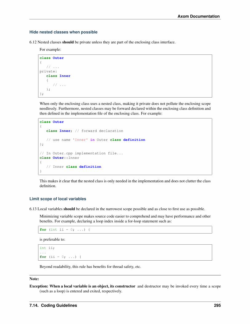
Axom Documentation

Hide nested classes when possible

6.12 Nested classes should be private unless they are part of the enclosing class interface.

For example:

class Outer

// ...private:

class Inner

// ...;

;

When only the enclosing class uses a nested class, making it private does not pollute the enclosing scopeneedlessly. Furthermore, nested classes may be forward declared within the enclosing class definition andthen defined in the implementation file of the enclosing class. For example:

class Outer

class Inner; // forward declaration

// use name 'Inner' in Outer class definition;

// In Outer.cpp implementation file...class Outer::Inner

// Inner class definition

This makes it clear that the nested class is only needed in the implementation and does not clutter the classdefinition.

Limit scope of local variables

6.13 Local variables should be declared in the narrowest scope possible and as close to first use as possible.

Minimizing variable scope makes source code easier to comprehend and may have performance and otherbenefits. For example, declaring a loop index inside a for-loop statement such as:

for (int ii = 0; ...)

is preferable to:

int ii;...for (ii = 0; ...)

Beyond readability, this rule has benefits for thread safety, etc.

Note:

Exception: When a local variable is an object, its constructor and destructor may be invoked every time a scope(such as a loop) is entered and exited, respectively.


Axom Documentation

Thus, instead of this:

for (int ii = 0; ii < 1000000; ++ii) Foo f;f.doSomethingCool(ii);

it may be more efficient to do this:

Foo f;for (int ii = 0; ii < 1000000; ++ii)

f.doSomethingCool(ii);

6.14 A local reference to any item in the global namespace (which should be rare if needed at all) should use the scopeoperator (“::”) to make the fact that it resides in the global namespace clear.

For example:

int local_val = ::global_val;

7.14.7 7 Code Documentation

This section contains guidelines for content and formatting of code documentation mentioned in earlier sections. Theaims of these guidelines are to:

• Document files, data types, functions, etc. consistently.

• Promote good documentation practices so that essential information is presented clearly and lucidly, and whichdo not over-burden developers.

• Generate source code documentation using the Doxygen system.

Document only what’s needed

7.1 Documentation should only include what is essential for users and other developers to easily understand code.Comments should be limited to describing constraints, pre- and post-conditions, and other issues that are important,but not obvious. Extraneous comments (e.g., documenting “the obvious”) should be avoided.

Code that uses clear, descriptive names (functions, variables, etc.) and clear logical structure is preferableto code that relies on a lot of comments for understanding. To be useful, comments must be understood byothers and kept current with the actual code. Generally, maintenance and understanding are better servedby rewriting tricky, unclear code than by adding comments to it.

Documenting new code vs. existing code

7.2 New source code must be documented following the guidelines in this section. Documentation of existing codeshould be modified to conform to these guidelines when appropriate.

7.3 Existing code documentation should be improved when its inadequate, incorrect, or unclear.

Note: When code is modified, documentation must be changed to reflect the changes.


Axom Documentation

Write clear documentation

7.4 To make comment text clear and reduce confusion, code comments should be written in grammatically-correctcomplete sentences or easily understood sentence fragments.

Documentation should be easy to spot

7.5 End-of-line comments should not be used to document code logic, since they tend to be less visible than othercomment forms and may be difficult to format cleanly.

Short end-of-line comments may be useful for labeling closing braces associated with nested loops, con-ditionals, for scope in general, and for documenting local variable declarations.

7.6 All comments, except end-of-line comments, should be indented to match the indentation of the code they aredocumenting. Multiple line comment blocks should be aligned vertically on the left.

7.7 Comments should be clearly delimited from executable code with blank lines and “blocking characters” (seeexamples below) to make them stand out and, thus, improve the chances they will be read.

7.8 White space, such as blank lines, indentation, and vertical alignment should be used in comment blocks to enhancereadability, emphasize important information, etc.

General Doxygen usage

The Doxygen code documentation system uses C or C++ style comment sections with special markings and Doxygen-specific commands to extract documentation from source and header files. Although Doxygen provides many sophis-ticated documentation capabilities and can generate a source code manual in a variety of formats such as LaTeX, PDF,and HTML, these guidelines address only a small subset of Doxygen syntax. The goal of adhering to a small, simpleset of documentation commands is that developers will be encouraged to build useful documentation when they arewriting code.

Brief vs. detailed comments

The Doxygen system interprets each documentation comment as either “brief” or “detailed”.

• A brief comment is a concise statement of purpose for an item (usually no more than one line) and starts withthe Doxygen command “\brief” (or “@brief”). Brief comments appear in summary sections of the generateddocumentation. They are typically seen before detailed comments when scanning the documentation; thus goodbrief comments make it easier to can or navigate a source code manual.

• A detailed comment is any comment that is not identified as ‘brief’.

7.9 A “brief” description should be provided in the Doxygen comment section for each of the following items:

• A type definition (i.e., class, struct, typedef, enum, etc.)

• A macro definition

• A struct field or class data member

• A class member function declaration (in the header file class definition)

• An unbound function signature (in a header file)

• A function implementation (when there is no description in the associated header file)

7.10 Important information of a more lengthy nature (e.g., usage examples spanning multiple lines) should be providedfor files, major data types and definitions, functions, etc. when needed. A detailed comment must be separated froma brief comment in the same comment block with a line containing no documentation text.


Axom Documentation

Doxygen comment blocks

7.11 Doxygen comment blocks may use either JavaDoc, Qt style, or one of the C++ comment forms described below.

JavaDoc style comments consist of a C-style comment block starting with two *’s, like this:

/*** ...comment text...

*/

Qt style comments add an exclamation mark (!) after the opening of a C-style comment block,like this:

/*!

* ...comment text...

*/

For JavaDoc or Qt style comments, the asterisk characters (“*”) on intermediate lines are optional, butencouraged.

C++ comment block forms start each line with an additional slash:

////// ...comment text...///

or an exclamation mark:

//!//! ...comment text...//!

For these C++ style comment forms, the comment delimiter is required on each line.

7.12 A consistent Doxygen comment block style must be used within a component.

7.13 Doxygen comment blocks must appear immediately before the items they describe; i.e., no blank lines betweencomment and documented item. This insures that Doxygen will properly associate the comment with the item.

Doxygen inline comments

7.14 Inline Doxygen comments may be used for class/struct data members, enum values, function arguments, etc.

When inline comments are used, they must appear after the item on the same line and must use thefollowing syntax:

/*!< ...comment text... */

Note that the “<” character must appear immediately after the opening of the Doxygen comment (withno space before). This tells Doxygen that the comment applies to the item immediately preceding thecomment. See examples in later sections.

7.15 When an item is documented using the inline form, the comment should not span multiple lines.

Copyright and release statement

7.16 Each file must contain a comment section that includes the project software release information (using whichevercomment characters are appropriate for the language the file is written in). In the interest of brevity, the complete


Axom Documentation

release statement is summarized here to show the essential information. The full version can be found in any of theproject files.

Note: Change this when we release the code.

/** Copyright (c) 2017-2022, Lawrence Livermore National Security, LLC.

* Produced at the Lawrence Livermore National Laboratory.

** All rights reserved.

** This source code cannot be distributed without permission and

* further review from Lawrence Livermore National Laboratory.

*/

See Header file layout details and Source file layout details for guidelines on placement of copyright and releasestatement in header and source files, respectively.

File documentation

7.17 Each header file that declares a global type, method, etc. must have a Doxygen file prologue similar to thefollowing:

/*!

***************************************************************************** \file ...optional name of file...

** \brief A brief statement describing the file contents/purpose. (optional)

** Optional detailed explanatory notes about the file.

******************************************************************************/

The "\\file" command **must** appear first in the file prologue. Itidentifies the comment section as documentation for the file.

The file name **may** include (part of) the path if the file name is notunique. If the file name is omitted on the line after the "\\file"command, then any documentation in the comment block will belong tothe file in which it is located instead of the summary documentationin the listing of documented files.

Note: Doxygen requires that a file itself must be documented for documentation to be generated for any global item(global function, typedef, enum, etc.) defined in the file.

See Header file layout details and Source file layout details for guidelines on placement of file prologue in header andsource files, respectively.


Axom Documentation

Brief and detailed comments

7.18 A brief statement of purpose for the file should appear as the first comment after the file command. If included,the brief statement, must be preceded by the “\brief” command.

7.19 Any detailed notes about the file may be included after the brief comment. If this is done, the detailed commentsmust be separated from the brief statement by a line containing no documentation text.

Type documentation

7.20 Each type and macro definition appearing in a header file must have a Doxygen type definition comment prologueimmediately before it. For example

/*!

****************************************************************************** \brief A brief statement of purpose of the type or macro.

** Optional detailed information that is helpful in understanding the

* purpose, usage, etc. of the type/macro ...

** \sa optional cross-reference to other types, functions, etc...

* \sa etc...

** \warning This class is only partially functional.

******************************************************************************/

Note: Doxygen requires that a compound entity, such as a class, struct, etc. be documented in order to document anyof its members.


7.21 A brief statement describing the type must appear as the first text comment using the Doxygen command “\brief”.

7.22 Important details about the item should be included after the brief comment and, if included, must be separatedfrom the brief comment by a blank line.

Cross-references and caveats

7.23 Cross-references to other items, such as other related types should be included in the prologue to enhance thenavigability of the documentation.

The Doxygen command “\sa” (for “see also”) should appear before each such cross-reference so thatlinks are generated in the documentation.

7.24 Caveats or limitations about the documented type should be noted using the “\warning” Doxygen command asshown above.


Axom Documentation

Function documentation

7.25 Each unbound function should be be documented with a function prologue in the header file where its prototypeappears or in a source file immediately preceding its implementation.

7.26 Since C++ class member functions define the class interface, they should be documented with a function prologueimmediately preceding their declaration in the class definition.

Example function documentation

The following examples show two function prologue variations that may be used to document a method in a classdefinition. The first shows how to document the function arguments in the function prologue.

/*!

*************************************************************************** \brief Initialize a Foo object with given operation mode.

** The "read" mode means one thing, while "write" mode means another.

** \return bool indicating success or failure of initialization.

* Success returns true, failure returns false.

** \param[in] mode OpMode enum value specifying initialization mode.

* ReadMode and WriteMode are valid options.

* Any other value generates a warning message and the

* failure value ("false") is returned.

***************************************************************************/bool initMode(OpMode mode);

The second example shows how to document the function argument inline.

/*!

************************************************************************** @brief Initialize a Foo object to given operation mode.

** The "read" mode means one thing, while "write" mode means another.

** @return bool value indicating success or failure of initialization.

* Success returns true, failure returns false.

***************************************************************************/bool initMode(OpMode mode /*!< [in] ReadMode, WriteMode are valid options */ );

Note that the first example uses the “" character to identify Doxygen commands; the second uses “@”.


7.27 A brief statement of purpose for a function must appear as the first text comment after the Doxygen command“\brief” (or “@brief”).


Axom Documentation

7.28 Any detailed function description, when included, must appear after the brief comment and must be separatedfrom the brief comment by a line containing no text.

Return values

7.29 If the function has a non-void return type, the return value should be documented in the prologue using theDoxygen command “\return” (or “@return”) preceding a description of the return value.

Functions with “void” return type and C++ class constructors and destructors should not have such doc-umentation.

Arguments

7.30 Function arguments should be documented in the function prologue or inline (as shown above) when the intentor usage of the arguments is not obvious.

The inline form of the comment may be preferable when the argument documentation is short. When alonger description is provided (such as when noting the range of valid values, error conditions, etc.) thedescription should be placed within the function prologue for readability. However, the two alternativesfor documenting function arguments must not be mixed within the documentation of a single function toreduce confusion.

In any case, superfluous documentation should be avoided. For example, when there are one or twoarguments and their meaning is obvious from their names or the description of the function, providing nocomments is better than cluttering the code by documenting the obvious. Comments that impart no usefulinformation are distracting and less helpful than no comment at all.

7.31 When a function argument is documented in the prologue comment section, the Doxygen command “param”should appear before the comment as in the first example above.

7.32 The “in/out” status of each function argument should be documented.

The Doxygen “param” command supports this directly by allowing such an attribute to be specified as“param[in]”, “param[out]”, or “param[in,out]”. Although the inline comment form does not support this,such a description should be included; e.g., by using “[in]”, “[out]”, or “[in,out]” in the comment.

Grouping small functions

7.33 Short, simple functions (e.g., inline methods) may be grouped together and documented with a single descriptivecomment when this is sufficient.

An example of Doxygen syntax for such a grouping is:

//@//! @name Setters for data members

void setMember1(int arg1) m_member1 = arg1; void setMember2(int arg2) m_member2 = arg2;

//@


Axom Documentation

Header file vs. source file documentation

7.34 Important implementation details (vs. usage detailed) about a function should be documented in the source filewhere the function is implemented, rather than the header file where the function is declared.

Header file documentation should include only purpose and usage information germane to an interface.When a function has separate implementation documentation, the comments must not contain Doxygensyntax. Using Doxygen syntax to document an item in more than one location (e.g., header file and sourcefile) can cause undesired Doxygen formatting issues and potentially confusing documentation.

A member of a class may be documented as follows in the source file for the class as follows (i.e., noDoxygen comments):

/************************************************************************** Set operation mode for a Foo object.

** Important detailed information about what the function does...

*************************************************************************/bool Foo::initMode(OpMode mode)

...function body...

Data member documentation

7.35 Each struct field or class data member should have a descriptive comment indicating its purpose.

This comment may as appear as a prologue before the item, such as:

/*!

* \brief Brief statement describing the input mode...

** Optional detailed information about the input mode...

*/int m_input_mode;

or, it may appear after the item as an inline comment such as:

int m_input_mode; /*!< \brief Brief statement describing the input mode....→˓*/


7.36 Regardless of which documentation form is used, a brief description must be included using the Doxygen com-mand “\brief” (or “@brief”).

7.37 Any detailed description of an item, if included, must appear after the brief comment and be separated from thebrief comment with a line containing no documentation text.

When a detailed comment is provided, or the brief statement requires more than one line, the prologuecomment form should be used instead of the inline form to make the documentation easier to read.


Axom Documentation

Grouping data members

7.38 If the names of data members are sufficiently clear that their meaning and purpose are obvious to other developers(which should be determined in a code review), then the members may be grouped together and documented with asingle descriptive comment.

An example of Doxygen syntax for such a grouping is:

//@//! @name Data member description...

int m_member1;int m_member2;...//@

Summary of common Doxygen commands

This Section provides an overview of commonly used Doxygen commands. Please see the Doxygen guide for moredetails and information about other commands.

Note that to be processed properly, Doxygen commands must be preceded with either “" or “@” character. For brevity,we use “" for all commands described here.

\brief The “brief” command is used to begin a brief description of a documented item. The brief descrip-tion ends at the next blank line.

\file The “file” command is used to document a file. Doxygen requires that to document any global item(function, typedef, enum, etc.), the file in which it is defined must be documented.

\name The “name” command, followed by a name containing no blank spaces, is used to define a namethat can be referred to elsewhere in the documentation (via a link).

\param The “param” command documents a function parameter/argument. It is followed by the param-eter name and description. The “\param” command can be given an optional attribute to indicateusage of the function argument; possible values are “[in]”, “[out]”, and “[in,out]”.

\return The “return” command is used to describe the return value of a function.

\sa The “sa” command (i.e., “see also”) is used to refer (and provide a link to) another documented item.It is followed by the target of the reference (e.g., class/struct name, function name, documentationpage, etc.).

@,@ These two-character sequences begin and end a grouping of documented items. Optionally, thegroup can be given a name using the “name” command. Groups are useful for providing additionalorganization in the documentation, and also when several items can be documented with a singledescription (e.g., a set of simple, related functions).

\verbatim, \endverbatim The “verbatim/endverbatim” commands are used to start/stop a block of textthat is to appear exactly as it is typed, without additional formatting, in the generated documentation.

-, -# The “-” and “-#” symbols begin an item in a bulleted list or numbered list, respectively. In eithercase, the item ends at the next blank line or next item.

\b, \e These symbols are used to make the next word bold or emphasized/italicized, respectively, in thegenerated documentation.



Axom Documentation

7.14.8 8 Design and Implement for Correctness and Robustness

The guidelines in this section describe various software design and implementation practices that help enforce correct-ness and robustness and avoid mis-interpretation or confusion by others.

Keep it simple. . .

8.1 Simplicity, clarity, ease of modification and extension should always be a main goal when writing new code orchanging existing code.

8.2 Each entity (class, struct, variable, function, etc.) should embody one clear, well-defined concept.

The responsibilities of an entity may increase as it is used in new and different ways. However, changesthat divert it from its original intent should be avoided. Also, large, monolithic entities that provide toomuch functionality or which include too many concepts tend to increase code coupling and complexity andintroduce undesirable side effects. Smaller, clearly constrained objects are easier to write, test, maintain,and use correctly. Also, small, simple objects tend to get used more often and reduce code redundancy.

Avoid global and static data

8.3 Global, complex, or opaque data sharing should not be used. Shared data increases coupling and contentionbetween different parts of a code base, which makes maintenance and modification difficult.

8.4 Static or global variables of class type must not be used.

Due to indeterminate order of construction, their use may cause bugs that are very hard to find. Static orglobal variables that are pointers to class types may be used and must be initialized properly in a singlesource file.

Avoid macros and magic numbers for constants

8.5 Preprocessor macros should not be used when there is a better alternative, such as an inline function or a constantvariable definition.

For example, this:

const double PI = 3.1415926535897932384626433832;

is preferable to this:

#define PI (3.1415926535897932384626433832)

Macros circumvent the ability of a compiler to enforce beneficial language concepts such as scope andtype safety. Macros are also context-specific and can produce errors that cannot be understood easily in adebugger. Macros should be used only when there is no better choice for a particular situation.

8.6 Hard-coded numerical constants and other “magic numbers” must not be used directly in source code. When suchvalues are needed, they should be declared as named constants to enhance code readability and consistency.

Avoid issues with compiler-generated class methods

The guidelines in this section apply to class methods that may be automatically generated by a compiler, includingconstructors, destructors, copy, and move methods. Developers should be aware of the conditions under which com-pilers will and will not generate these methods. Developers should also be aware of when compiler-generated methodssuffice and when they do not. After providing some guidelines, we discuss standard C++ rules that compilers follow for


Axom Documentation

generating class methods when they are not explicitly defined. See Understand standard rules for compiler-generatedmethods.

The most important cases to pay attention to involve the destructor, copy constructor, and copy-assignment operator.Classes that provide these methods, either explicitly or compiler-generated, are referred to as copyable. Failing tofollow the rules for these methods can be damaging due to errors or unexpected behavior. Rules involving the moveconstructor and move-assignment operator are less important since they mostly affect efficiency and not correctness.Copy operations can be used to accomplish the same end result as move operations, just less efficiently. Move se-mantics are an important optimization feature of C++. The C++11 standard requires compilers to use move operationsinstead of copy operations when certain conditions are fulfilled. Classes that provide move operations, either explicitlyor compiler-generated, are referred to as movable.

Rule of three

8.7 Each class must follow the Rule of Three which states: if the destructor, copy constructor, or copy-assignmentoperator is explicitly defined, then the others must be defined.

Compiler-generated and explicit versions of these methods must not be mixed. If a class requires one ofthese methods to be implemented, it almost certainly requires all three to be implemented.

This rule helps guarantee that class resources are managed properly. C++ copies and copy-assigns ob-jects of user-defined types in various situations (e.g., passing/returning by value, container manipulations,etc.). These special member functions will be called, if accessible. If they are not user-defined, they areimplicitly-defined by the compiler.

Compiler-generated special member functions can be incorrect if a class manages a resource whose handleis an object of non-class type. Consider a class data member which is a bare pointer to an object. Thecompiler-generated class destructor will not free the object. Also, the compiler-generated copy constructorand copy-assignment operator will perform a “shallow copy”; i.e., they will copy the value of the pointerwithout duplicating the underlying resource.

Neglecting to free a pointer or perform a deep copy when those operations are expected can result inserious logic errors. Following the Rule of Three guards against such errors. On the rare occasion theseactions are intentional, a programmer-written destructor, copy constructor, and copy-assignment operatorare ideal places to document intent of design decisions.

Restrict copying of non-copyable resources

8.8 A class that manages non-copyable resources through non-copyable handles, such as pointers, should declare thecopy methods private and and leave them unimplemented.

When the intent is that such methods should never be called, this is a good way to help a compiler to catchunintended usage. For example:

class MyClass

// ...

private:DISABLE_DEFAULT_CTOR(MyClass);DISABLE_COPY_AND_ASSIGNMENT(MyClass);

// ...;


Axom Documentation

When code does not have access to the private members of a class tries to use such a method, a compile-time error will result. If a class does have private access and tries to use one of these methods an link-timeerror will result.

This is another application of the “Rule of Three”.

Please see 10 Common Code Development Macros, Types, etc. for more information about the macrosused in this example to disable compiler-generated methods.

Note: Exception: If a class inherits from a base class that declares these methods private, the subclass need notdeclare the methods private. Including comments in the derived class header indicating that the the parent classenforces the non-copyable properties of the class is helpful.

Rely on compiler-generated methods when appropriate

8.9 When the compiler-generated methods are appropriate (i.e., correct and sufficiently fast), the default constructor,copy constructor, destructor, and copy assignment may be left undeclared. In this case, it is often helpful to addcomments to the class header file indicating that the compiler-generated versions of these methods will be used.

8.10 If a class is default-constructable and has POD (“plain old data”) or pointer data members, a default constructorshould be provided explicitly and its data members must be initialized explicitly if a default constructor is provided.A compiler-generated default constructor will not initialize such members, in general, and so will leave a constructedobject in an undefined state.

For example, the following class should provide a default constructor and initialize its data members in it:

class MyClass

MyClass();

// ...

private:double* m_dvals;int[] m_ivals;

;

Functors should always be copyable

8.11 By convention, a functor class should have a copy constructor and copy-assignment operator.

Typically, the compiler-generated versions are sufficient when the class has no state or non-POD datamembers. Since such classes are usually small and simple, the compiler-generated versions of thesemethods may be used without documenting the use of default value semantics in the functor definition.

For example:

class MyFunctor

// Compiler-generated copy ctor and copy assignment sufficient

private:DIABLE_DEFAULT_CTOR(MyFunctor); // prevent default construction



Axom Documentation


// ...;

Note that in this example, the default constructor is disabled to prevent default construction. This can help prevent pro-gramming errors when object state must be fully initialialized on construction. For more information about commonAxom macros, see 10 Common Code Development Macros, Types, etc..

Understand standard rules for compiler-generated methods

This section provides some background information related to the guidelines in the previous section. There, weprovide guidelines that help to decide when to define class methods that may be generated automatically by a compilerand when relying on compiler-generated versions suffices. Here, we describe the conditions under which compilersgenerate methods automatically.

Consider the following simple class:

class MyClasspublic:

int x;;

How many methods does it have? None?

Actually, MyClass may have as many as six methods depending on how it is used: a default constructor, destructor,copy constructor, copy-assignment operator, move constructor, and move-assignment operator. Any of these may begenerated by a compiler.

Note: See 11 Portability, Compilation, and Dependencies for discussion about using C++11 features such as movesemantics.

C++ compiler rules for generating class member functions are:

• The parameter-less default constructor is generated if a class does not define any constructor and all base classesand data members are default-constructable. This means that once you declare a copy constructor (perhaps todisable the automatically provided one), the compiler will not supply a default constructor.

• The destructor is automatically supplied if possible, based on the members and the base classes.

• A copy constructor is generated if all base classes and members are copy-constructable. Note that referencemembers are copy-constructable.

• The copy-assignment operator is generated if all base classes and members are copy-assignable. For this pur-pose, reference members are not considered copy-assignable.

• A move constructor is supplied unless the class has any of the following: a user-defined copy constructor, copy-assignment operator, move-assignment operator, or destructor. If the move constructor cannot be implementedbecause not all base classes or members are move-constructable, the supplied move constructor will be definedas deleted.

• A move-assignment operator is generated under the same conditions as the move constructor.

The importance of understanding these rules and applying the guidelines in the previous section is underscored by thefact that compiler-generated methods may have different behaviors depending on how they are used. Here we providesome examples based on MyClass defined above.


Axom Documentation

If MyClass has a user-defined constructor, then

MyClass item1;

and

MyClass item2 = MyClass();

will both call the user-defined default constructor “MyClass()” and there is only one behavior.

However, if MyClass relies on the compiler-generated constructor

MyClass item1;

performs default initialization, while

MyClass item2 = MyClass();

performs value initialization.

Default initialization calls the constructors of any base classes, and nothing else. Since constructors for intrinsic typesdo not do anything, that means all member variables will have garbage values; specifically, whatever values happen toreside in the corresponding addresses.

Value initialization also calls the constructors of any base classes. Then, one of two things happens:

• If MyClass is a POD class (all member variables are either intrinsic types or classes that only contain intrinsictypes and have no user-defined constructor/destructor), all data is initialized to 0.

• If MyClass is not a POD class, the constructor does not touch any data, which is the same as default initialization(so member variables have garbage values unless explicitly constructed otherwise).

Other points worth noting:

• Intrinsic types, such as int, float, bool, pointers, etc. have constructors that do nothing (not even initialize tozero), destructors that do nothing, and copy constructors and copy assignment-ers that blindly copy bytes.

• Comparison operators, such as “==” or “!=” are never automatically generated by a compiler, even if all baseclasses and members are comparable.

Initializing and copying class members

Initialize all members at construction

8.12 Class type variables should be defined using direct initialization instead of copy initialization to avoid unwantedand spurious type conversions and constructor calls that may be generated by compilers.

For example, use:

std::string name("Bill");

instead of:

std::string name = "Bill";

or:

std::string name = std::string("Bill");


Axom Documentation

8.13 Each class data member must be initialized (using default values when appropriate) in every class constructor.That is, an initializer or initialization must be provided for each class data member so that every object is in a well-defined state upon construction.

Generally, this requires a user-defined default constructor when a class has POD members. Do not assumethat a compiler-generated default constructor will leave any member variable in a well-defined state.

Note: Exception: A class that has no data members, including one that is derived from a base class with a de-fault constructor that provides full member initialization, does not require a user-defined default constructor since thecompiler-generated version will suffice.

Know when to use initialization vs. assignment

8.14 Data member initialization should be used instead of assignment in constructors, especially for small classes.Initialization prevents needless run-time work and is often faster.

8.15 When using initialization instead of assignment to set data member values in a constructor, data members shouldalways be initialized in the order in which they appear in the class definition.

Compilers adhere to this order regardless of the order that members appear in the class initialization list.So you may as well agree with the compiler rules and avoid potential errors that could result when onemember depends on the state of another.

8.16 For classes with complex data members, assignment within the body of the constructor may be preferable.

If the initialization process is sufficiently complex, it may be better to initialize (i.e., assign) memberobjects in a method that is called after object creation, such as “init()”.

Use the copy-and-swap idiom

8.17 A user-supplied implementation of a class copy-assignment operator should check for assignment to self, mustcopy all data members from the object passed to operator, and must return a reference to “*this”.

The copy-and-swap idiom should be used.

Initializing, copying, and inheritance

8.18 A constructor must not call a virtual function on any data member object since an overridden method defined ina subclass cannot be called until the object is fully constructed.

There is no general guarantee that data members are fully-created before a constructor exits.

8.19 All constructors and copy operations for a derived class must call the necessary constructors and copy operationsfor each of its base classes to insure that each object is properly allocated and initialized.

Prefer composition to inheritance

8.20 Class composition should be used instead of inheritance to extend behavior.

Looser coupling between objects is typically more flexible and easier to maintain and refactor.


Axom Documentation

Keep inheritance relationships simple

8.21 Class hierarchies should be designed so that subclasses inherit from abstract interfaces; i.e., pure virtual baseclasses.

Inheritance is often done to reuse code that exists in a base class. However, there are usually better designchoices to achieve reuse. Good object-oriented use of inheritance is to reuse existing calling code byexploiting base class interfaces using polymorphism. Put another way, “interface inheritance” should beused instead of “implementation inheritance”.

8.22 Deep inheritance hierarchies; i.e., more than 2 or 3 levels, should be avoided.

8.23 Multiple inheritance should be restricted so that only one base class contains methods that are not “pure virtual”.

8.24 “Private” and “protected” inheritance must not be used unless you absolutely understand the ramifications ofsuch a choice and are sure that it will not create design and implementation problems.

Such a choice must be reviewed with team members. There almost always exist better alternatives.

Design for/against inheritance

8.25 One should not inherit from a class that was not designed to be a base class; e.g., if it does not have a virtualdestructor.

Doing so is bad practice and can cause problems that may not be reported by a compiler; e.g., hiding baseclass members. To add functionality, one should employ class composition rather than by “tweaking” anexisting class.

8.26 The destructor of a class that is designed to be a base class must be declared “virtual”.

However, sometimes a destructor should not be declared virtual, such as when deletion through a pointerto a base class object should be disallowed.

Use virtual functions responsibly

8.27 Virtual functions should be overridden responsibly. That is, the pre- and post-conditions, default arguments, etc.of the virtual functions should be preserved.

Also, the behavior of an overridden virtual function should not deviate from the intent of the base class.Remember that derived classes are subsets, not supersets, of their base classes.

8.28 Inherited non-virtual methods must not be overloaded or hidden.

8.29 A virtual function in a base class should only be implemented in the base class if its behavior is always validdefault behavior for any derived class.

8.30 If a method in a base class is not expected to be overridden in any derived class, then the method should not bedeclared virtual.

8.31 If each derived class has to provide specific behavior for a base class virtual function, then it should be declaredpure virtual.

8.32 Virtual functions must not be called in a class constructor or destructor. Doing so is undefined behavior. Even ifit seems to work correctly, it is fragile and potentially non-portable.

Inline functions

Function inlining is a compile time operation and the full definition of an inline function must be seen wherever it iscalled. Thus, the implementation of every function to be inlined must be provided in a header file.


Axom Documentation

Whether or not a function implemented in a header file is explicitly declared inline using the “inline” keyword, thecompiler decides if the function will be inlined. A compiler will not inline a function that it considers too long ortoo complex (e.g., if it contains complicated conditional logic). When a compiler inlines a function, it replaces thefunction call with the body of the function. Most modern compilers do a good job of deciding when inlining is a goodchoice.

It is possible to specify function attributes and compiler flags that can force a compiler to inline a function. Suchoptions should be applied with care to prevent excessive inlining that may cause executable code bloat and/or maymake debugging difficult.

Note: When in doubt, don’t use the “inline” keyword and let the compiler decide whether to inline a function.

Inline short, simple functions

8.33 Simple, short frequently called functions, such as accessors, that will almost certainly be inlined by most compil-ers should be implemented inline in header files.

Only inline a class constructor when it makes sense

8.34 Class constructors should not be inlined in most cases.

A class constructor implicitly calls the constructors for its base classes and initializes some or all of itsdata members, potentially calling more constructors. If a constructor is inlined, the construction andinitialization needed for its members and bases will appear at every object declaration.

Note: Exception: A class/struct that has only POD members, is not a subclass, and does not explicitly declare adestructor, can have its constructor safely inlined in most cases.

Do not inline virtual methods

8.35 Virtual functions must not be inlined due to polymorphism.

For example, do not declare a virtual class member function as:

inline virtual void foo( )

In most circumstances, a virtual method cannot be inlined because a compiler must do runtime dispatchon a virtual method when it doesn’t know the complete type at compile time.

Note: Exception: It is safe to define an empty destructor inline in an abstract base class with no data members.

Important: Should we add something about C++11 ‘final’ keyword???

Function and operator overloading


Axom Documentation

There’s a fine line between clever and. . .

8.36 Operator overloading must not be used to be clever to the point of obfuscation and cause others to think too hardabout an operation. Specifically, an overloaded operator must preserve “natural” semantics by appealing to commonconventions and must have meaning similar to non-overloaded operators of the same name.

Overloading operators can be beneficial, but should not be overused or abused. Operator overloadingis essentially “syntactic sugar” and an overloaded operator is just a function like any other function. Animportant benefit of overloading is that it often allows more appropriate syntax that more easily commu-nicates the meaning of an operation. The resulting code can be easier to write, maintain, and understand,and it may be more efficient since it may allow the compiler to take advantage of longer expressions thanit could otherwise.

Overload consistently

8.37 Function overloading must not be used to define functions that do conceptually different things.

Someone reading declarations of overloaded functions should be able to assume (and rightfully so!) thatfunctions with the same name do something very similar.

8.38 If an overloaded virtual method in a base class is overridden in a derived class, all overloaded methods with thesame name in the base class must be overridden in the derived class.

This prevents unexpected behavior when calling such member functions. Remember that when a virtualfunction is overridden, the overloads of that function in the base class are not visible to the derived class.

Common operators

8.39 Both boolean operators “==” and “!=” should be implemented if one of them is.

For consistency and correctness, the “!=” operator should be implemented using the “==” operator im-plementation. For example:

bool MyClass::operator!= (const MyClass& rhs)

return !(this == rhs);

8.40 Standard operators, such as “&&”, “||”, and “,” (i.e., comma), must not be overloaded.

Built-in versions of these operators are typically treated specially by a compiler. Thus, programmerscannot implement their full semantics. This can cause confusion. For example, the order of operandevaluation cannot be guaranteed when overloading operators “&&” or “||”. This may cause problems assomeone may write code that assumes that evaluation order is the same as the built-in versions.

Function arguments

Consistent argument order makes interfaces easier to use

8.41 Function arguments must be ordered similarly for all routines in an Axom component.

Common conventions are either to put all input arguments first, then outputs, or vice versa. Input andoutput arguments must not be mixed in a function signature. Parameters that are both input and output


Axom Documentation

can make the best choice unclear. Conventions consistent with related functions must always be fol-lowed. When adding a new parameter to an existing method, the established ordering convention must befollowed.

Note: When adding an argument to an existing method, do not just stick it at the end of the argument list.

Pointer and reference arguments and const

8.42 Each function argument that is not a built-in type (i.e., int, double, char, etc.) should be passed either by referenceor as a pointer to avoid unnecessary copies.

8.43 Each function reference or pointer argument that is not changed by the function must be declared “const”.

Always name function arguments

8.44 Each argument in a function declaration must be given a name that exactly matches the function implementation.

For example, use:

void computeSomething(int op_count, int mode);

not:

void computeSomething(int, int);

Function return points

8.45 Each function should have exactly one return point to make control logic clear.

Functions with multiple return points tend to be a source of errors when trying to understand or modifycode, especially if there are multiple return points within a scope. Such code can always be refactored tohave a single return point by using local scope boolean variables and/or different control logic.

A function may have two return points if the first return statement is associated with error condition check,for example. In this case, the error check should be performed at the start of the function body beforeother statements are reached. For example, the following is a reasonable use of two function return pointsbecause the error condition check and the return value for successful completion are clearly visible:

int computeSomething(int in_val)

if (in_val < 0) return -1;

// ...rest of function implementation...

return 0;

Note: Exception. If multiple return points actually fit well into the logical structure of some code, they may be used.For example, a routine may contain extended if/else conditional logic with several “if-else” clauses. If needed, thecode may be more clear if each clause contains a return point.


Axom Documentation

Proper type usage

8.46 The “bool” type should be used instead of “int” for boolean true/false values.

8.47 The “string” type should be used instead of “char*”.

The string type supports and optimizes many character string manipulation operations which can be error-prone and less efficient if implemented explicitly using “char*” and standard C library functions. Notethat “string” and “char*” types are easily interchangeable, which allows C++ string data to be used wheninteracting with C routines.

8.48 An enumeration type should be used instead of macro definitions or “int” data for sets of related constant values.

Since C++ enums are distinct types with a compile-time specified set of values, there values cannot beimplicitly cast to integers or vice versa – a “static_cast” operator must be used to make the conversionexplicit. Thus, enums provide type and value safety and scoping benefits.

In many cases, the C++11 enum class construct should be used since it provides stronger type safety andbetter scoping than regular enum types.

Templates

8.49 A class or function should only be made a template when its implementation is independent of the template typeparameter.

Note that class member templates (e.g., member functions that are templates of a class that is not atemplate) are often useful to reduce code redundancy.

8.50 Generic templates that have external linkage must be defined in the header file where they are declared sincetemplate instantiation is a compile time operation. Implementations of class templates and member templates that arenon-trivial should be placed in the class header file after the class definition.

Use const to enforce correct usage

8.51 The “const” qualifier should be used for variables and methods when appropriate to clearly indicate usage and totake advantage of compiler-based error-checking. For example, any class member function that does not change thestate of the object on which it is called should be declared “const”

Constant declarations can make code safer and less error-prone since they enforce intent at compile time.They also improve code understanding because a constant declaration clearly indicates that the state of avariable or object will not change in the scope in which the declaration appears.

8.52 Any class member function that does not change a data member of the associated class must be declared “const”.

This enables the compiler to detect unintended usage.

8.53 Any class member function that returns a class data member that should not be changed by the caller must bedeclared “const” and must return the data member as a “const” reference or pointer.

Often, both “const” and non-“const” versions of member access functions are needed so that callers maydeclare the variable that holds the return value with the appropriate “const-ness”.

Casts and type conversions

Avoid C-style casts, const_cast, and reinterpret_cast

8.54 C-style casts must not be used.


Axom Documentation

All type conversions must be done explicitly using the named C++ casting operators; i.e., “static_cast”,“const_cast”, “dynamic_cast”, “reinterpret_cast”.

8.55 The “const_cast” operator should be avoided.

Casting away “const-ness” is usually a poor programming decision and can introduce errors.

Note: Exception: It may be necessary in some circumstances to cast away const-ness, such as when calling const-incorrect APIs.

8.56 The “reinterpret_cast” must not be used unless absolutely necessary.

This operator was designed to perform a low-level reinterpretation of the bit pattern of an operand. Thisis needed only in special circumstances and circumvents type safety.

Use the explicit qualifier to avoid unwanted conversions

8.57 A class constructor that takes a single non-default argument, or a single argument with a default value, must bedeclared “explicit”.

This prevents compilers from performing unexpected (and, in many cases, unwanted!) implicit typeconversions. For example:

class MyClasspublic:

explicit MyClass(int i, double x = 0.0);;

Note that, without the explicit declaration, an implicit conversion from an integer to an object of typeMyClass could be allowed. For example:

MyClass mc = 2;

Clearly, this is confusing. The “explicit” keyword forces the following usage pattern:

MyClass mc(2);

to get the same result, which is much more clear.

Memory management

Allocate and deallocate memory in the same scope

8.58 Memory should be deallocated in the same scope in which it is allocated.

8.59 All memory allocated in a class constructor should be deallocated in the class destructor.

Note that the intent of constructors is to acquire resources and the intent of destructors is to free thoseresources.

8.60 Pointers should be set to null explicitly when memory is deallocated. This makes it easy to check pointers for“null-ness” when needed.


Axom Documentation

Use new/delete consistently

8.61 Data managed exclusively within C++ code must be allocated and deallocated using the “new” and “delete”operators.

The operator “new” is type-safe, simpler to use, and less error-prone than the “malloc” family of C func-tions. C++ new/delete operators must not be combined with C malloc/free functions.

8.62 Every C++ array deallocation statement must include “[ ]” (i.e., “delete[ ]”) to avoid memory leaks.

The rule of thumb is: when “[ ]” appears in the allocation, then “[ ]” must appear in the correspondingdeallocation statement.

7.14.9 9 Code Formatting

Conditional statements and loops

9.1 Curly braces should be used in all conditionals, loops, etc. even when the content inside the braces is a “one-liner”.

This helps prevent coding errors and misinterpretation of intent. For example, this:

if (done) ...

is preferable to this:

if (done) ...

9.2 One-liners may be used for “if” conditionals with “else/else if” clauses when the resulting code is clear.

For example, either of the following styles may be used:

if (done) id = 3;

else id = 0;

or:

if (done) id = 3; else id = 0;

9.3 Complex “if/else if” conditionals with many “else if” clauses should be avoided.

Such statements can always be refactored using local boolean variables or “switch” statements. Doing sooften makes code easier to read and understand and may improve performance.

9.4 An explicit test for zero/nonzero must be used in a conditional unless the tested quantity is a boolean or pointertype.

For example, a conditional based on an integer value should use:

if (num_lines != 0) ...

not:

if (num_lines) ...


Axom Documentation

White space and code alignment

Most conventions for indentation, spacing and code alignment preferred by the team are enforced by using the clang-format tool.

There are several build system targets related to code formatting grouped under the check and style targets. The formerverify that the code is properly formatted, while the latter modify source files to conform to axom’s rules.

Important: Axom’s style targets modify source files. Please ensure that you’ve committed/staged all your changesbefore running them.

Tip: When axom is configured to use the make-based generator, the entire codebase can be formatted by runningmake clangformat_style from the build directory. Simiarly, one can verify that the code if properly formattedby running make clangformat_check. There are also component-specific variants for these targets, e.g. foraxom’s core component, we have core_clangformat_style and core_clangformat_check.

Not all preferred formatting conventions are supported by clang-format. The following guidelines provide additionalrecommendations to make code easier to read and understand.

White space enhances code readability

9.5 Blank lines and indentation should be used throughout code to enhance readability.

Examples of helpful white space include:

• Between operands and operators in arithmetic expressions.

• After reserved words, such as “while”, “for”, “if”, “switch”, etc. and before the parenthesis or curlybrace that follows.

• After commas separating arguments in functions.

• After semi-colons in for-loop expressions.

• Before and after curly braces in almost all cases.

9.6 White space must not appear between a function name and the opening parenthesis to the argument list. Inparticular, if a function call is broken across source lines, the break must not come between the function name and theopening parenthesis.

9.7 Tabs must not be used for indentation since this can be problematic for developers with different text editorsettings.

Vertical alignment helps to show scope

9.8 When function arguments (in either a declaration or implementation) appear on multiple lines, the argumentsshould be vertically aligned for readability.

9.9 All statements within a function body should be indented within the surrounding curly braces.

9.10 All source lines in the same scope should be vertically aligned. Continuation of previous lines may be indentedif it make the code easier to read.


Axom Documentation

Break lines where it makes sense

9.11 When a line is broken at a comma or semi-colon, it should be broken after the comma or semi-colon, not before.This helps make it clear that the statement continues on the next line.

9.12 When a source line is broken at an arithmetic operator (i.e., +, -, etc.), it should be broken after the operator, notbefore.

Use parentheses for clarity

9.13 Parentheses should be used in non-trivial mathematical and logical expressions to clearly indicate structure andintended order of operations. Do not assume everyone who reads the code knows all the rules for operator precedence.

7.14.10 10 Common Code Development Macros, Types, etc.

This section provides guidelines for consistent use of macros and types defined in Axom components, such as“axom_utils” and “slic”, and in our build system that we use in day-to-day code development.

Important: Code that is guarded with macros described in this section must not change the externally-observableexecution behavior of the code.

The macros are intended to help users and developers avoid unintended or potentially erroneous usage, etc. not confusethem.

Unused variables

10.2 To silence compiler warnings and express variable usage intent more clearly, macros in the AxomMacros.hppheader file in the source include directory must be used when appropriate. For example,:

void my_function(int x, int AXOM_DEBUG_PARAM(y))

// use variable y only for debug compilation

Here, the AXOM_DEBUG_PARAM macro indicates that the variable ‘y’ is only used when the code is compiled indebug mode. It also removes the variable name in the argument list in non-debug compilation to prevent unwantedcompiler warnings.

Please see the AxomMacros.hpp header file for other available macros and usage examples.

Disabling compiler-generated methods

10.3 To disable compiler-generated class/struct methods when this is desired and to clearly express this intent, theAXOMMacros.hpp header file in source include directory contains macros that should be used for this purpose. SeeAvoid issues with compiler-generated class methods for more information about compiler-generated methods.

Please see the AXOMMacros.hpp header file for other available macros and usage examples.


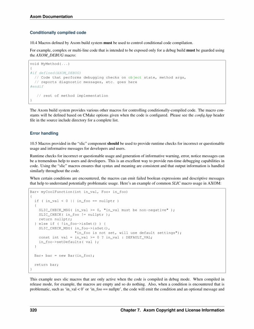
Axom Documentation

Conditionally compiled code

10.4 Macros defined by Axom build system must be used to control conditional code compilation.

For example, complex or multi-line code that is intended to be exposed only for a debug build must be guarded usingthe AXOM_DEBUG macro:

void MyMethod(...)#if defined(AXOM_DEBUG)

// Code that performs debugging checks on object state, method args,// reports diagnostic messages, etc. goes here

#endif

// rest of method implementation

The Axom build system provides various other macros for controlling conditionally-compiled code. The macro con-stants will be defined based on CMake options given when the code is configured. Please see the config.hpp headerfile in the source include directory for a complete list.

Error handling

10.5 Macros provided in the “slic” component should be used to provide runtime checks for incorrect or questionableusage and informative messages for developers and users.

Runtime checks for incorrect or questionable usage and generation of informative warning, error, notice messages canbe a tremendous help to users and developers. This is an excellent way to provide run-time debugging capabilities incode. Using the “slic” macros ensures that syntax and meaning are consistent and that output information is handledsimilarly throughout the code.

When certain conditions are encountered, the macros can emit failed boolean expressions and descriptive messagesthat help to understand potentially problematic usage. Here’s an example of common SLIC macro usage in AXOM:

Bar* myCoolFunction(int in_val, Foo* in_foo)

if ( in_val < 0 || in_foo == nullptr )SLIC_CHECK_MSG( in_val >= 0, "in_val must be non-negative" );SLIC_CHECK( in_foo != nullptr );return nullptr;

else if ( !in_foo->isSet() ) SLIC_CHECK_MSG( in_foo->isSet(),

"in_foo is not set, will use default settings");const int val = in_val >= 0 ? in_val : DEFAULT_VAL;in_foo->setDefaults( val );

Bar* bar = new Bar(in_foo);

return bar;

This example uses slic macros that are only active when the code is compiled in debug mode. When compiled inrelease mode, for example, the macros are empty and so do nothing. Also, when a condition is encountered that isproblematic, such as ‘in_val < 0’ or ‘in_foo == nullptr’, the code will emit the condition and an optional message and


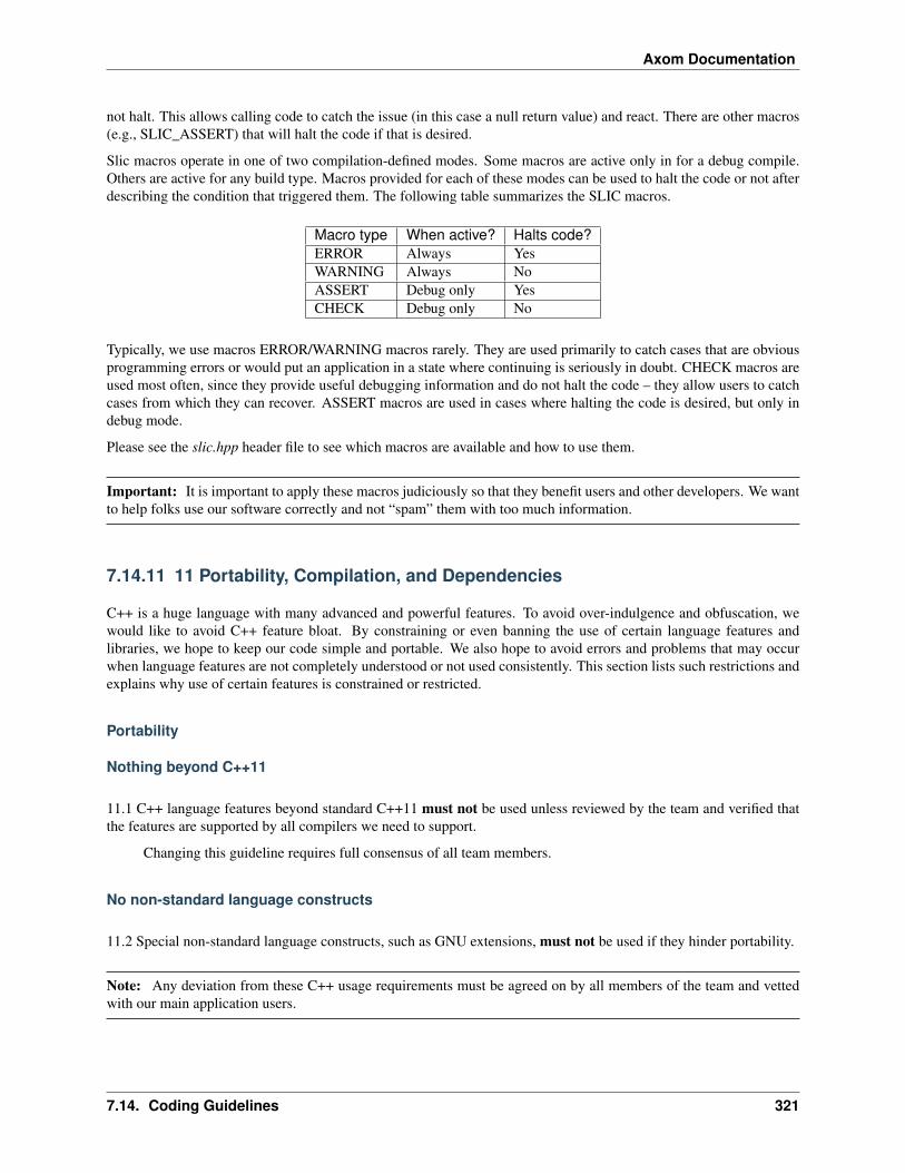
Axom Documentation

not halt. This allows calling code to catch the issue (in this case a null return value) and react. There are other macros(e.g., SLIC_ASSERT) that will halt the code if that is desired.

Slic macros operate in one of two compilation-defined modes. Some macros are active only in for a debug compile.Others are active for any build type. Macros provided for each of these modes can be used to halt the code or not afterdescribing the condition that triggered them. The following table summarizes the SLIC macros.

Macro type When active? Halts code?ERROR Always YesWARNING Always NoASSERT Debug only YesCHECK Debug only No

Typically, we use macros ERROR/WARNING macros rarely. They are used primarily to catch cases that are obviousprogramming errors or would put an application in a state where continuing is seriously in doubt. CHECK macros areused most often, since they provide useful debugging information and do not halt the code – they allow users to catchcases from which they can recover. ASSERT macros are used in cases where halting the code is desired, but only indebug mode.

Please see the slic.hpp header file to see which macros are available and how to use them.

Important: It is important to apply these macros judiciously so that they benefit users and other developers. We wantto help folks use our software correctly and not “spam” them with too much information.

7.14.11 11 Portability, Compilation, and Dependencies

C++ is a huge language with many advanced and powerful features. To avoid over-indulgence and obfuscation, wewould like to avoid C++ feature bloat. By constraining or even banning the use of certain language features andlibraries, we hope to keep our code simple and portable. We also hope to avoid errors and problems that may occurwhen language features are not completely understood or not used consistently. This section lists such restrictions andexplains why use of certain features is constrained or restricted.

Portability

Nothing beyond C++11

11.1 C++ language features beyond standard C++11 must not be used unless reviewed by the team and verified thatthe features are supported by all compilers we need to support.

Changing this guideline requires full consensus of all team members.

No non-standard language constructs

11.2 Special non-standard language constructs, such as GNU extensions, must not be used if they hinder portability.

Note: Any deviation from these C++ usage requirements must be agreed on by all members of the team and vettedwith our main application users.


Axom Documentation

Compilation

Avoid conditional compilation

11.3 Excessive use of the preprocessor for conditional compilation at a fine granularity (e.g., selectively including orremoving individual source lines) should be avoided.

While it may seem convenient, this practice typically produces confusing and error-prone code. Often, itis better to refactor the code into separate routines or large code blocks subject to conditional compilationwhere it is more clear.

Code reviews by team members will dictate what is/is not acceptable.

The compiler is your friend

11.4 Developers should rely on compile-time and link-time errors to check for code correctness and invariants.

Errors that occur at run-time and which depend on specific control flow and program state are inconvenientfor users and can be difficult to detect and fix.

Important: Add specific guidance on how this should be done. . .

Minimize dependencies on third-party libraries (TPLs)

11.5 While it is generally desirable to avoid recreating functionality that others have already implemented, we shouldlimit third-party library dependencies for Axom to make it easier for users. We are a library, and everything wenecessarily depend on will become a dependency for our user.

Before introducing any significant TPL dependency on Axom (e.g., hdf5), it must be agreed on bythe development team and vetted with our main users.

11.6 Unless absolutely necessary, any TPL we depend on must not be exposed through any public interface in Axom.

7.14.12 References and Useful Resources

Most of the guidelines here were gathered from the following list sources. The list contains a variety of useful resourcesfor programming in C++ beyond what is presented in these guidelines.

1. The Chromium Projects: C++ Dos and Don’ts. https://chromium.googlesource.com/chromium/src/+/HEAD/styleguide/c++/c++-dos-and-donts.md

2. Dewhurst, S., C++ Gotchas: Avoiding Common Problems in Coding and Design, Addison-Wesley, 2003.

3. Dewhurst S., C++ Common Knowledge: Essential Intermediate Programming, Addison-Wesley, 2005.

4. Doxygen manual, http://www.doxygen.nl/manual/

5. Google C++ Style Guide, https://google.github.io/styleguide/cppguide.html

6. ISO/IEC 14882:2011 C++ Programming Language Standard.

7. Josuttis, N., The C++ Standard Library: A Tutorial and Reference, Second Edition, Addison-Wesley, 2012.

8. LLVM Coding Standards, llvm.org/docs/CodingStandards.html

9. Meyers, S., More Effective C++: 35 New Ways to Improve Your Programs and Designs, Addison-Wesley, 1996.


https://chromium.googlesource.com/chromium/src/+/HEAD/styleguide/c++/c++-dos-and-donts.md

https://chromium.googlesource.com/chromium/src/+/HEAD/styleguide/c++/c++-dos-and-donts.md


https://google.github.io/styleguide/cppguide.html

Axom Documentation

10. Meyers, S., Effective STL: 50 Specific Ways to Improve Your Use of the Standard Template Library, Addison-Wesley, 2001.

11. Meyers, S., Effective C++: 55 Specific Ways to Improve Your Programs and Designs (3rd Edition), Addison-Wesley, 2005.

12. Meyers, S., Effective Modern C++: 42 Specific Ways to Improve Your Use of C++11 and C++14, O’Reilly.

13. Programming Research Ltd., High-integrity C++ Coding Standard, Version 4.0, 2013.

14. Sutter, H. and A. Alexandrescu, C++ Coding Standards: 101 Rules, Guidelines, and Best Practices, Addison-Wesley, 2005.

7.15 License Info

7.15.1 Axom License

Copyright (c) 2017-2022, Lawrence Livermore National Security, LLC. All rights reserved.

Redistribution and use in source and binary forms, with or without modification, are permitted provided that thefollowing conditions are met:

• Redistributions of source code must retain the above copyright notice, this list of conditions and the followingdisclaimer.

• Redistributions in binary form must reproduce the above copyright notice, this list of conditions and the follow-ing disclaimer in the documentation and/or other materials provided with the distribution.

• Neither the name of the copyright holder nor the names of its contributors may be used to endorse or promoteproducts derived from this software without specific prior written permission.

THIS SOFTWARE IS PROVIDED BY THE COPYRIGHT HOLDERS AND CONTRIBUTORS “AS IS” AND ANYEXPRESS OR IMPLIED WARRANTIES, INCLUDING, BUT NOT LIMITED TO, THE IMPLIED WARRANTIESOF MERCHANTABILITY AND FITNESS FOR A PARTICULAR PURPOSE ARE DISCLAIMED. IN NO EVENTSHALL THE COPYRIGHT HOLDER OR CONTRIBUTORS BE LIABLE FOR ANY DIRECT, INDIRECT, IN-CIDENTAL, SPECIAL, EXEMPLARY, OR CONSEQUENTIAL DAMAGES (INCLUDING, BUT NOT LIMITEDTO, PROCUREMENT OF SUBSTITUTE GOODS OR SERVICES; LOSS OF USE, DATA, OR PROFITS; OR BUSI-NESS INTERRUPTION) HOWEVER CAUSED AND ON ANY THEORY OF LIABILITY, WHETHER IN CON-TRACT, STRICT LIABILITY, OR TORT (INCLUDING NEGLIGENCE OR OTHERWISE) ARISING IN ANYWAY OUT OF THE USE OF THIS SOFTWARE, EVEN IF ADVISED OF THE POSSIBILITY OF SUCH DAM-AGE.

7.15. License Info 323

Axom Documentation

Documents

Transcript of Axom Documentation