Axiomatizing Congestion Control

33

Axiomatizing Congestion Control

DORON ZARCHY, Hebrew University of Jerusalem

RADHIKA MITTAL, University of Illinois at Urbana-Champaign

MICHAEL SCHAPIRA, Hebrew University of Jerusalem

SCOTT SHENKER, UC Berkeley, ICSI

The overwhelmingly large design space of congestion control protocols, along with the increasingly diverse

range of application environments, makes evaluating such protocols a daunting task. Simulation and experi-

ments are very helpful in evaluating the performance of designs in specific contexts, but give limited insight

into the more general properties of these schemes and provide no information about the inherent limits of

congestion control designs (such as, which properties are simultaneously achievable and which are mutually

exclusive). In contrast, traditional theoretical approaches are typically focused on the design of protocols that

achieve to specific, predetermined objectives (e.g., network utility maximization), or the analysis of specific

protocols (e.g., from control-theoretic perspectives), as opposed to the inherent tensions/derivations between

desired properties.

To complement today’s prevalent experimental and theoretical approaches, we put forth a novel principled

framework for reasoning about congestion control protocols, which is inspired by the axiomatic approach from

social choice theory and game theory. We consider several natural requirements (“axioms”) from congestion

control protocols – e.g., efficient resource-utilization, loss-avoidance, fairness, stability, and TCP-friendliness –

and investigate which combinations of these can be achieved within a single design. Thus, our framework

allows us to investigate the fundamental tradeoffs between desiderata, and to identify where existing and new

congestion control architectures fit within the space of possible outcomes.

CCS Concepts: • Networks → Network protocols;

ACM Reference Format:Doron Zarchy, Radhika Mittal, Michael Schapira, and Scott Shenker. 2019. Axiomatizing Congestion Control.

Proc. ACM Meas. Anal. Comput. Syst. 3, 2, Article 33 (June 2019), 33 pages. https://doi.org/10.1145/3326148

1 IntroductionRecent years have witnessed a revival of both industrial and academic interest in improving

congestion control designs. The quest for better congestion control is complicated by the extreme

diversity and range of (i) the design space (as exemplified by the stark conceptual and operational

differences between recent proposals [8, 14, 18, 19, 49, 50]), (ii) the desired properties (ranging from

high performance to fairness to TCP-friendliness), (iii) the envisioned operational setting (inter-

and intra-datacenter, wireless, the commercial Internet, satellite), and (iv) the application loads and

requirements (small vs. large traffic demands, latency- vs. bandwidth-sensitive).Most congestion control research uses simulation and experiments under a limited range of

network conditions. This is extremely important for understanding the detailed performance of

Authors’ addresses: Doron Zarchy, Hebrew University of Jerusalem, [email protected]; Radhika Mittal, University of

Illinois at Urbana-Champaign, [email protected]; Michael Schapira, Hebrew University of Jerusalem, schapiram@huji.

ac.il; Scott Shenker, UC Berkeley, ICSI, [email protected].

Permission to make digital or hard copies of all or part of this work for personal or classroom use is granted without fee

provided that copies are not made or distributed for profit or commercial advantage and that copies bear this notice and

the full citation on the first page. Copyrights for components of this work owned by others than ACM must be honored.

Abstracting with credit is permitted. To copy otherwise, or republish, to post on servers or to redistribute to lists, requires

prior specific permission and/or a fee. Request permissions from [email protected].

© 2019 Association for Computing Machinery.

2476-1249/2019/6-ART33 $15.00

https://doi.org/10.1145/3326148

Proc. ACM Meas. Anal. Comput. Syst., Vol. 3, No. 2, Article 33. Publication date: June 2019.

https://doi.org/10.1145/3326148

https://doi.org/10.1145/3326148

33:2 Doron Zarchy, Radhika Mittal, Michael Schapira, and Scott Shenker

particular schemes in specific settings, but provides limited insight into the more general properties

of these schemes and no information about the inherent limits (such as, which properties are

simultaneously achievable and which are mutually exclusive). In contrast, traditional theoretical

approaches are typically focused on the design of protocols that achieve specific, predetermined

objectives (e.g., network utility maximization [26, 46]), or the analysis of specific protocols (e.g., from

control-theoretic perspectives [1, 37]), as opposed to exploring the inherent tensions/derivations

between desired properties.

We advocate an axiomatic approach to congestion control, which is complementary to the

experimental and theoretical work currently being pursued. Our approach, modeled on similar

efforts in social choice theory and game theory [7], identifies a set of requirements (“axioms”) and

then identifies (i) which of its subsets of requirements can coexist (i.e., there are designs that achieve

all of them) and which subsets cannot be met simultaneously (i.e., no design can simultaneouslyachieve all of them), and (ii) whether some requirements immediately follow from satisfying other

requirements. Thus, the axiomatic approach can shed light on the inherent tradeoffs involved in

congestion control protocol design, and can be leveraged to classify existing and proposed solutions

according to the properties they satisfy.

The axiomatic approach has been applied tomany computer science environments, e.g. reputation

systems [47], recommendation systems [6], link prediction [17], and networking environments [17,

28, 42]. To the best of our knowledge, ours is the first application of this approach to congestion

control protocols (though [42] touches on the subject briefly).

We introduce a simple network model where we can evaluate congestion control designs and

formulate several natural axioms (or requirements) for congestion control protocols, including

efficient link-utilization, loss-avoidance, fairness, stability, and TCP-friendliness. Congestion control

protocols can be regarded as points in a multidimensional space reflecting the extent to which they

satisfy these requirements, and we show how classical families of congestion control protocols (e.g.,

additive-increase-multiplicative-decrease [16, 53], multiplicative-increase-multiplicative-decrease,

and more) can be mapped to points in this space.

We leverage our axiomatic framework to derive basic results on the feasibility of simultaneouslyachieving different requirements within a single design. Our results formalize and shed light on

various empirical/experimental observations about tensions between different desiderata, including

(1) the tension between attaining high performance and being friendly to legacy TCP connec-

tions [27, 36], (2) the tension between achieving high bandwidth and maintaining low latency under

dynamic environments [11, 32, 50], and (3) the tension between being robust to non-congestion loss

and not incurring high loss upon convergence [19]. From a protocol design perspective, desirable

congestion control protocols are those that reside on the Pareto frontier in the multidimensional

space induced by our requirements, and this Pareto frontier is characterized by our theoretical

results.

To be sure, our axiomatic approach has its limitations, as it revolves around investigating these

properties in a simplified model. However, we feel that the results, in terms of which axioms

can coexist and which cannot, provide insights that apply far beyond the simple model (even if

the detailed theoretical results do not). Thus, we contend that the axiomatic approach is a useful

addition to the evaluatory arsenal that researchers should apply to congestion control.

Organization. In the following section, we introduce the simple network model we use to evaluate

congestion control designs and discuss its limitations. Then, in Section 3, we formulate several

natural axioms (or requirements) for congestion control protocols, including efficient link-utilization,

loss-avoidance, fairness, stability, and TCP-friendliness. In Section 4, we derive our basic results on


Axiomatizing Congestion Control 33:3

the feasibility of achieving these requirements and then, in Section 5, we show the mapping from

congestion control protocols to points in a multidimensional space.

2 Modeling Protocol DynamicsWe consider a simple model of dynamics of congestion control protocols (which builds upon [9,

16, 36]). We show below that studying our simple (and tractable) model gives rise to interesting

insights about the fundamental tradeoffs involved in congestion control protocol design. We also

discuss the limitations of our model.

Senders dynamically interacting on a link. n senders 1, . . .n send traffic on a link of bandwidth

B > 0 (measured in units of MSS/s), propagation delay Θ, and buffer size τ (measured in units

of MSS).1In our model, B, Θ, and τ are all unknown to the senders, precluding the possibility of

building into protocols a priori assumptions, such as “the link is only shared by senders running

protocol P”, “the minimum latency is at least 2ms”, etc. We let C = B × 2Θ, i.e., C represents the

minimum possible bandwidth-delay product for the link, or its “capacity”. Senders experience

synchronized feedback. Time in our model is regarded as an infinite sequence of discrete time steps

t = 0, 1, 2, . . ., each of RTT duration, in which end-host (sender) decisions occur. At the beginning

of each time step t , sender i can adjust its congestion window by selecting a value in the range

{0, 1, . . . ,M}, in units of MSS. We assume that 1 << M . Let x (t )i denote the size of the sender i’s

congestion window at time t , let x̄ (t ) = (x (t )1, . . . ,x (t )n ), and let X (t ) =

∑i x

(t )i .

The duration of time step t , RTT (t), is a function of the link’s propagation delay and the buffer’s

queuing delay. This is captured (as in [27, 31, 53]) as follows:

RTT (x̄ (t ),C,τ ) =

max(2Θ, X

(t )−CB + 2Θ),

if X (t ) < C + τ

∆, otherwise

(1)

where ∆ represents a timeout-triggered cap on the RTT in the event of packet loss.

When traffic sent on the link at time t exceeds C + τ , excess traffic is dropped according to the

FIFO (droptail) queuing policy. The loss rate experienced by each sender at time step t as a functionof the congestion window sizes of all senders and the link capacity and buffer size, is captured as:

L(x̄ (t ),C,τ ) =

{(1 − C+τ

X (t ) ) if X (t ) > C + τ

0 otherwise

(2)

To simplify exposition, we will denote the loss rate at time t simply by L(t ).

Congestion control protocols and the induced dynamics. Each sender i’s selection of congestion-window sizes is dictated by the congestion control protocol Pi employed by that sender. A congestion

control protocol (deterministically) maps the history of congestion-window sizes of that sender, and

of the RTTs and loss rates experienced by that sender, to the sender’s next selection of congestion

window size. A protocol is loss-based if its choice of window-sizes is invariant to the RTT values.

Any choice of initial congestion windows x̄ (0) = (x (0)1, . . . ,x (0)n ) and congestion control protocol Pi

for each sender i induces a dynamic of congestion control as follows: senders start sending as in

x̄ (0) and, at each time step, every sender i repeatedly reacts to its environment as prescribed by Pi .Protocols belonging to the families of Additive-Increase-Multiplicative-Decrease (AIMD(a,b)

[21, 52]) and Multiplicative-Increase-Multiplicative-Decrease (MIMD(a,b) [4, 5]) are easy to model

in our framework: AIMD(a,b) increases the window size x (t )i additively by a (MSS) if the loss L(t ) attime t is 0, whereas MIMD(a,b) increases the window size multiplicatively by a factor of a. Both

1MSS (maximum segment size) is the maximum number of bytes in a single TCP segment.

protocols multiplicatively decrease the window size by a factor of b if L(t ) > 0. We formalize two

more prominent families of protocols within our model: Binomial [9], and TCP Cubic [24].

A binomial protocol BIN(a,b,k, l) for a > 0, 0 0

TCP Cubic, CUBIC(c,b), can be captured as follows:

x (t+1)

i =

{xmaxi + c(T − (

xmaxi (1−b)

c )1

3 )3 if L(t ) = 0

xmaxi b if L(t ) > 0

where xmaxi is the window size of sender i when the last packet loss was experienced, T is the

number of time steps elapsed from the last packet loss, b ∈ (0, 1) is the rate-decrease factor, andc > 0 is a scaling factor.

Limitations of model. Clearly, our model does not capture many of the intricacies of congestion

control. However, as will be shown in the sequel, our model encompasses many scenarios of interest,

and trends revealed by our axiomatic investigation are also reflected in our experimental findings.

Aspects whose incorporation into our model is left for future research include: (1) Extending our

model and results to network-wide dynamics (as opposed to competition over a single bottleneck

link)2. (2) Modeling the effects of queuing at routers by incorporating ideas from queueing theory

and control theory. (3) Examining other queueing policies (beyond the prevalent droptail), such as

RED [10], WFQ [44], and SPQ [29]. (4) Extending our model to non-synchronized feedback [43, 51].

(5) Modeling slow-starts and timeouts. (6) Transitioning from a fluid-level model to a packet-

level model to better capture, e.g., low-rate transmissions. (7) Extending our protocol formulation

to incorporate randomized protocols. (8) Extending our model to pacing-based (as opposed to

window-based) protocols (e.g., PCC [18, 19] and BBR [14]).

3 Axiomatic ApproachWe consider eight natural requirements (“axioms”) from congestion control protocols. Intuitively,

these requirements capture the desiderata of well-utilizing spare network resources, avoiding ex-

cessive loss, achieving fairness amongst competing flows, converging to a stable rate-configuration,

attaining high-performance in the presence of non-congestion loss [14], being friendly towards

legacy TCP connections, and not suffering excessive latency. However, what precisely is the def-

inition of “well-utilizing a link”? Is it utilizing 90% of the link from some point onwards? 95%?

What does it mean to be friendly to TCP? Is it not to exceed by over 1.5x the throughput of a TCPconnection sharing the same link? 3x?

Different choices of values to plug into our requirements (resulting in different formulations of

axioms) can have significant implications, to the extent of opposite answers to questions regarding

whether two (or more) requirements can be satisfied simultaneously. To allow for a nuanced

discussion of the interplay between axioms, instead of reasoning about axioms with hardwired

constants, we parameterize the requirements (turning them into “metrics”).

A congestion control protocol can be regarded as a point in the 8-dimensional space induced by

the following metrics, according to its “score” in each metric.

2Importantly, reasoning about network-wide dynamics of congestion control is highly challenging even for fixed-ratesenders [23].

Metric I: efficiency. We say that a congestion-control protocol P is α -efficient if when all senders

employ P , for any initial configuration of senders’ window sizes, there is some time step T such

that from T onwards X (t ) ≥ αC .

Metric II: fast-utilization.Our next metric is intended to exclude protocols that take an unreason-

able amount of time to utilize spare bandwidth (e.g., that increase the window size by a single MSS

every 1, 000 RTTs). Intuitively, the following definition of α-fast-utilization captures the property

that, for any “long enough” time period, the protocol consumes link capacity at least as fast as

a protocol that increases the congestion window by α MSS in each RTT. A congestion-control

protocol P is α-fast-utilizing if there exists T > 0 such that if a P-sender i’s window size is x (t1)

i at

time step t1 and by time step t1 + ∆t , for any ∆t ≥ T , does not experience loss, nor increased RTT

(if not loss-based), then Σt1+∆tt=t1

(x (t )i − x (t1)

i ) ≥α∆2

t2.

Metric III: loss-avoidance.We say that a congestion-control protocol P is α -loss-avoiding if, whenall senders employ P , for any initial configuration of senders’ window sizes, there is some time

step T such that from T onwards the loss rate L(t ) is bounded by α (e.g., α = 0.01 translates to not

exceeding loss rate of 1%). We refer to protocols that are 0-loss-avoiding, i.e., protocols that, from

some point onwards, do not incur loss, as “0-loss”.

Metric IV: fairness. We say that a congestion-control protocol P is α -fair if when all senders use

P and for any configuration of senders’ window sizes, from some time T > 0 onwards, the average

window size of each sender i is at least an α-fraction that of any other sender j.

Metric V: convergence.We say that a congestion-control protocol P is α -convergent, for α ∈ [0, 1],if there is a configuration of window sizes (x∗

1, . . . ,x∗n) ∈ [0,M]n and time step T such that for any

t > T and sender i ∈ N , αx∗i ≤ x (t )i ≤ (2 − α)x∗i (e.g., α = 0.9 means that from some point onwards

the window sizes are within 10% from a fixed point).

Metric VI: robustness to non-congestion loss. A natural demand from congestion control

protocols is to be robust to loss that does not result from congestion [14, 18]. Clearly, formulating

this requirement in all possible contexts is challenging. We focus on a simple, yet enlightening,

scenario (used in [18] to motivate PCC): Suppose that a single sender i sends on a link of infinite

capacity (so as to remove from consideration congestion-based loss). We say that a protocol P is

α-robust if, when the sender experiences random packet loss rate of at most α ∈ [0, 1] at any time

t > 0 time, then, for any choice of initial senders’ window sizes, and for any value β > 0, there is

some T > 0 such that for every t̄ > T , x (t̄ )i ≥ β (i.e., non-congestion loss of rate at most α does not

prevent utilization of spare capacity).

Metric VII: TCP-friendliness.We say that a protocol P is α -friendly to another protocolQ if, for

any combination of sender-protocols such that some senders use P and others use Q , for everyinitial configuration of senders’ window sizes, and for every P-sender i and Q-sender j, from some

point in time T > 0 on wards, j’s average window size is at least an α-fraction of i’s averagewindow size. Observe that friendliness, as defined above, is closely related to fairness (Metric

IV), but fairness is with respect to many instantiations of the same protocol, whereas friendlinesscaptures interactions between different protocols. We say that a protocol P is α -TCP-friendly if P is

α-friendly towards AIMD(1,0.5) (i.e., TCP Reno).

Metric VIII: latency-avoidance.We say that protocol P is α-latency-avoiding if for sufficiently

large link capacity C and buffer size τ , and regardless of sender’s initial window sizes, when all

senders on the link employ P , there is some time stepT such that fromT onwardsRTT (t) < (1+α)2Θ.The term 2Θ captures the minimum possible RTT (twice the link’s propagation delay).


Why these metrics? As the above long list of metrics indicates, congestion control protocol

design is a remarkably complex task. Proposed protocols are expected to meet many requirements,

including optimizing multiple facets of locally-experienced performance (bandwidth utilization,

loss rate, self-induced latency), reaching desirable global outcomes (fast convergence, fairness), not

being overly aggressive to legacy TCP, and more. One of our key contributions is putting forth a

theoretical framework that formalizes these desiderata and enables both the investigation of their

interdependence, and the “scoring” of existing/proposed protocols. Our metrics formalize classical

requirements from congestion control protocols [20], which are often considered when evaluating

these protocols (see, e.g.,[8, 18, 19, 50]).

While our metrics capture intuitive interpretations of conventional requirements from congestion

control, clearly other formalizations of these metrics could be considered. Investigating how, within

our axiomatic framework, relaxing/modifying our metrics influences the possibility/impossibility

borderline for congestion control is important for informing protocol design. In social choice theory

and game theory, revisiting the axiomatic model of classical results (e.g., Arrow’s Theorem [7] and

the Gibbard-Satterthwaite Theorem [22]) has yielded valuable insights. Our metrics and results

thus constitute the first steps in such a discussion.

4 Axiomatic DerivationsWe present below theoretical results highlighting the intricate connections between ourmetrics. Our

results establish that some properties of a congestion control scheme are immediate consequences

of other properties or, conversely, cannot be satisfied in parallel to satisfying other properties. The

latter form of results exposes fundamental tensions between metrics, implying that attaining a

higher “score” in one metric inevitably comes at the expense lowering the score in another. We

leverage this insight in Section 5 to reason about the Pareto frontier for protocol design in the

8-dimensional metric space induced by our metrics.

4.1 Relating Axioms

We begin with the following simple observation:

Claim 1. Any loss-based protocol that is 0-loss is not α-fast-utilizing for any α > 0.

To see why the above is not obvious, consider a protocol P that slowly increases its rate until

encountering loss for the first time and then slightly decreases the rate so as to not exceed the link’s

capacity. While both 0-loss (from some point in time no loss occurs) and almost fully-utilizing the

link, this protocol is not α-fast-utilizing for any α > 0. The reason is that, for loss-based protocols,

α-fast-utilization implies after sufficiently long time without packet loss, the protocol must increase

its rate until encountering loss yet again. We now prove this formally.

Proof. (of Claim 1) Consider the scenario that a single sender is utilizing the link and employing

protocol P . Suppose that the sender is 0-loss-avoiding then after, sufficient time, its window size

must be upper bounded by some value H ≤ C + τ (otherwise a loss event occurs infinitely many

times). However, recall that any loss-based, α-fast-utilizing protocol P (for α > 0) is associated with

a time value T > 0 such that for any t1 > 0, if no loss event occurs in the time interval [t1, t1 +T ],

then

∑t1+Tt=t1

(x (t ) − x (t1)) ≥ αT 2

2. This implies that the P-sender must increase its window size by at

leastαT 2

2within the time period [t1, t1 +T ]. However, this implies that for any period of T̄ time

steps in which no loss event occurs, such thatαT 2

2MSS > (C + τ ) the sender must experience loss.

This contradicts the definition of the upper bound H . □

We present below other, more subtle, connections between our metrics. All of our bounds apply

across all possible network parameters (link capacity, buffer size) and number of senders, with the


exception of Theorem 3 (where the reliance on C and τ is explicit). We start with the following

result, which relates convergence, fast-utilization, and efficiency.

Theorem 1. Any protocol that is α-convergent and β-fast-utilizing, for some β > 0, is at leastα

2−α -efficient.

Proof. (of Theorem 1) Let protocol P be α-convergent and β-fast-utilizing, for some β > 0.

Suppose, for point of contradiction, that protocol P is notα

2−α -efficient. This implies that for any

T > 0 there is t > T such that ∑i ∈[n]

x (t )i <( α

2 − α

)C (3)

Since P is α-convergent, there exists a configuration of window sizes (x∗1, . . . ,x∗n) ∈ [0,M]n such

that after sufficient time T̃ , for each P sender i and for any t > T̃ ,

αx∗i ≤ x (t )i ≤ (2 − α)x∗i (4)

As P is β-fast-utilizing, the sum of senders’ rates must exceed the link capacity C , otherwise Pcan experience no loss and no latency increase indefinitely without increasing its rate, violating

the definition of β-fast-utilization. This, combined with (4), implies that for some large enough t

C <∑i

x (t )i ≤∑i

(2 − α)x∗i (5)

Equation (4) also implies that x∗i ≤x (t )iα .

Putting everything together yields that for infinitely many values of t

C < (2 − α)∑i

x∗i ≤ (2 − α)∑i

x (t )i

α=

=2 − α

α

∑i

x (t )i <2 − α

α×

α

2 − αC = C

—a contradiction. The theorem follows. □

4.2 Two Upper Bounds on TCP-Friendliness

We next present results showing that protocols that satisfy certain desiderata are upper bounded in

terms of their levels of TCP-friendliness.

Theorem 2. Any loss-based protocol that is α-fast-utilizing and β-efficient is at most 3(1−β )α (1+β ) -TCP-

friendly

Proof sketch for Theorem 2: To prove the theorem, we first establish that any loss-based protocol

that is α-fast-utilizing and β-efficient is no more TCP friendly than AIMD(α , β). Intuitively, thisis because AIMD(α , β) increases its rate at the minimal pace required to attain α-fast-utilization,and decreases its rate at the maximum pace required to not violate β-efficiency (thus freeing up

bandwidth for contending TCP flows). Our formalization of this intuition leverages arguments

similar to those in [13, 36] to reason about the duration of the time interval between two consecutive

loss events when the protocol under consideration and TCP Reno share the same link. The longer

the intervals the less TCP Reno’s aggressive backoff mechanism is triggered and so the less TCP

Reno’s throughput is harmed. We observe that AIMD(α , β) maximizes the length across all α-fast-utilizing and β-efficient protocols and is thus the friendliest to TCP among them. We then derive

the upper bound on the TCP-friendliness of α-fast-utilizing and β-efficient protocols simply by

upper bounding the friendliness of AIMD(α , β) towards TCP Reno (i.e., AIMD(1, 1

2)). We point out

that the upper bound on TCP-friendliness of Theorem 2 is, in fact, tight, asAIMD(α , β)) is precisely3(1−β )α (1+β ) -TCP-friendly (see also the analysis in [13]).

Theorem 3. Any loss-based protocol that is α-fast-utilizing, β-efficient, and ϵ-robust, for ϵ > 0, isat most

3(1−β )(4(C+τ

1−ϵ )−α )(1+β )-TCP friendly.

Proof sketch for Theorem 3: Similarly to the proof of Theorem 2, the proof of Theorem 3 also

relies on identifying a class of congestion control protocols, such that upper bounds on TCP-

friendliness for these protocols extend to all other protocols. Again, this involves reasoning about

the time intervals between consecutive loss events.

Specifically, we introduce a family of protocols, called Robust-AIMD, which can be regarded as a

hybrid of traditional AIMD and PCC [18]. Under Robust-AIMD, time is divided into short (roughly

1 RTT) “monitor intervals”. In each monitor interval, the sender sends at a certain rate and uses

selective ACKs from the receiver to learn the resulting loss rate. Robust-AIMD uses an AIMD-like

rule for adjusting transmission rate: the sender has a congestion window (similarly to TCP and

unlike PCC) that is additively increased by a predetermined constant a (MSS) if the experienced

loss rate is lower than a fixed constant ϵ > 0, and multiplicatively decreased by a predetermined

constant b if the loss rate exceeds ϵ . Thus, Robust-AIMD is modeled as follows. Robust-AIMD(a,b,ϵ):

x (t+1)

i =

{x (t )i + a if L(t ) < ϵ

x (t )i b if L(t ) ≥ ϵ

We show that any loss-based protocol that is α-fast-utilizing, β-efficient, and ϵ-robust, for ϵ > 0,

is at best as TCP-friendly as Robust-AIMD(α ,β ,ϵ) and upper bound the TCP-friendliness of the

latter.

Our analysis of Robust-AIMD(α ,β ,ϵ) reveals that the upper bound of Theorem 3 is tight for

ϵ << β , in the sense that Robust-AIMD(α ,β ,ϵ) exactly matches it, giving rise to the following result:

Theorem 4. For any α > 0, β > 0, and ϵ > 0 such that ϵ << β , there exists a protocol that isα-fast-utilizing, β-efficient, ϵ-robust, and 3(1−β )

(4(C+τ1−ϵ )−α )(1+β )

-TCP-friendly.

We will revisit Robust-AIMD when discussing the Pareto frontier for protocol design in Sec-

tion 5.2.

4.3 On Establishing TCP-Friendliness

Often, to establish that a congestion control protocol is TCP-friendly, simulation or experimental

results are presented to demonstrate that it does not harm TCP by “too much”. What, though,

guarantees that friendliness towards a certain TCP variant implies friendliness towards other TCP

variants? Our next result suggests a principled approach to establishing TCP-friendliness: prove

that the protocol is friendly towards a specific TCP variant (say, TCP Reno) and deduce that it is at

least as friendly to any “more aggressive” TCP variant. We introduce the following terminology: a

protocol P is more aggressive than a protocol Q if for any combination of P- and Q-senders, andinitial sending rates, from some point in time onwards, the average goodput of any P-sender ishigher than that of any Q-sender.

Theorem 5. Let P andQ be two protocols such that (1) each protocol is either AIMD, BIN, or MIMD,(2) P is α-TCP-friendly, and (3) Q is more aggressive than Reno. Then, P is α-friendly to Q .

AIMD and BIN are special cases for BIN [9]. Since BIN protocol converges to a steady state, all

BIN protocols can be ordered by their aggressiveness according to the sum l + k in the protocol

(where l and k are in the protocol specification)

4.4 Loss-based vs. Latency-Avoiding Protocols

Mo et al. show that the loss-based TCP Reno is very aggressive towards the latency-avoiding TCP

Vegas [32]. Intuitively, this is a consequence of Vegas backing off upon exceeding some latency

bound while Reno continues to increase its rate since it is oblivious to latency. The following result

shows that any “reasonable” loss-based protocol is extremely unfriendly towards any member of a

broad family of latency-avoiding protocols that includes TCP Vegas.

We say that a protocol is latency-decreasing if, for some fixed α > 0, when the experienced RTT

is not within an α-factor from the minimum possible RTT the sender must decrease its rate. Put

formally: if, for some time t , RTT (t) > α × 2Θ, then x (t+1)

i < x (t )i for every P-sender i . We point out

that TCP Vegas, which documents the minimum experienced RTT and decreases its rate when the

experienced RTT is “too high” with respect to that value, falls within this class of protocols (for the

appropriate choice of α ).

Theorem 6. For any α > 0 and β > 0, any loss-based protocol that is α-efficient is not β-friendlyto any latency-decreasing protocol.

Proof sketch for Theorem 6: Consider a loss-based protocol P that is α-efficient for some α > 0,

and a latency-decreasing protocolQ . Suppose that a single P-sender is sharing the link with a single

Q-sender. As Q is latency-decreasing, there exists some value δ such that when the experienced

RTT exceeds δ × 2Θ the Q-sender must decrease its rate. Now, let the size of the buffer τ be such

that the when the sum of sending rates is α(C + τ ) the RTT is strictly higher than δ × 2Θ. Considerthe scenario that the initial congestion window of P isC +τ and the initial congestion window ofQis 1 MSS, which is assumed to be negligible with respect to C + τ . This initial choice of congestionwindow sizes captures a scenario in which P-sender is fully utilizing the buffer when the Q-sender

starts sending (or, alternatively, the Q-sender experienced a timeout while the P-sender sends at ahigh rate). Our proof shows that henceforth, the congestion window of the P-sender will always belower bounded by α(C+τ ) and so the RTTwill always be at least δ×2Θ. Consequently, theQ-sender

cannot increase its congestion window and must send at its minimum rate. To see why, observe

that as P is loss-based, from the P-sender’s perspective, this environment is indistinguishable from

the environment in which the link capacity is C + τ and there is no buffer. In addition, so long as

the Q-sender sends at a fixed (its minimum) rate, the P-sender cannot distinguish between the

(actual) scenario that the link is shared with others and the scenario that the P-sender is alone onthe link. Consequently, α-efficiency dictates that the congestion window of the P-sender remain

of size at least α(C + τ ). This, in turn, by our choice of τ forces the Q-sender to not increase its

congestion window size. The theorem follows.

4.5 When Can Axioms Coexist?

Our axiomatic derivations above establish that certain desiderata cannot be simultaneously achieved

by loss-based protocols (see Claim 1, Theorem 2, and Theorem 3). Importantly, these impossibility

results hold regardless of the number of senders and network parameters (bandwidth, buffer

size, etc.). We show below that, in certain conditions, latency-sensitive protocols can bypass the

impossibility results of this section and, in fact, well-satisfy all of the requirements of Section 3.

However, as the discussion below illustrates, this is subtle and, in particular, depends on the

network parameters. Thus, going beyond the impossibility results of this section requires not


only considering congestion signals other than loss (latency) but also a more nuanced, parameter-

dependent, discussion.

To see this, consider the following protocol design, termed “AIMDl ”. Intuitively, AIMDl is the

latency-sensitive extension of AIMD (see Section 2). AIMDl gradually increases its rate so long

as no loss is experienced and its experienced latency does not increase. In the event that loss is

experienced, or the RTT increases, AIMDl decreases its rate. Specifically:

AIMDl (a,b):

x (t+1)

i =

{x (t )i + a if L(t ) = 0 or RTT (t) ≤ RTT (t − 1)

x (t )i b if L(t ) > 0 or RTT (t) > RTT (t − 1)

Consider first the scenario that the buffer size τ is very large. Intuitively, in this scenario, the

dynamics of congestion control are precisely as with AIMD(a,b)-senders on a link with no buffer,

as every time traffic enters the buffer the reactions of the AIMDl senders is identical to that of

AIMD senders experiencing loss. Consequently, in terms of efficiency, fairness, convergence, and

fast-utilization, AIMDl (a,b) exhibits the exact same guarantees as AIMD(a,b) (to be presented in

Table 1 of Section 5).

However, when the buffer size is very large, AIMDl can easily be shown to be 0-loss avoiding

(as it shies away from increased latency and so empties the buffer). In addition, AIMDl is very

TCP-friendly. In fact, being latency-decreasing (see Section 4), Theorem 6 applies to AIMDl and so

the loss-based TCP Reno is actually not friendly towards AIMDl . Thus, under these conditions,

AIMDl provides lower loss-avoidance (by Claim 1) and higher TCP-friendliness (by Theorem 6)

than achievable by any loss-based protocol.

Moreover, for “good” choices of a and b, say, a = 1 and b = 0.99, AIMDl can achieve “good

scores” in all these metrics but robustness. In fact, the analogously defined latency-sensitive variant

Robust-AIMDl of Robust-AIMD attains fairly high scored with respect to all eight requirements of

Section 3.

Observe, however, that when no buffer exists, or the buffer size τ is small, AIMDl and Robust-

AIMDl , now being effectively loss-based only, are reduced to AIMD and Robust-AIMD, respectively.

Consequently, these protocols are no longer 0 − loss , nor very TCP-friendly, in light of the impossi-

bility results of Claim 1, and Theorem 2, and Theorem 3.

5 Protocol Analysis and DesignOur theoretical framework, as presented in Section 2, allows us to associate each congestion control

protocol with a 8-tuple of real numbers, representing its scores in the eight metrics. We present

below our results in this direction and explain the implications for protocol design.

5.1 Mapping Protocols to Points

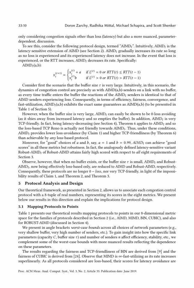
Table 1 presents our theoretical results mapping protocols to points in our 8-dimensional metric

space for the families of protocols described in Section 2 (i.e., AIMD, MIMD, BIN, CUBIC), and also

for ROBUST-AIMD (discussed in Section 4).

We present in angle brackets worst-case bounds across all choices of network parameters (e.g.,

very shallow buffer, very high number of senders, etc.). To gain insight into how the specific link

parameters (capacity C , buffer size τ ) and number of senders n affect efficiency, stability, etc., we

complement some of the worst-case bounds with more nuanced results reflecting the dependence

on these parameters.

The results regarding the fairness and TCP-friendliness of BIN are derived from [9] and the

fairness of CUBIC is derived from [24]. Observe that MIMD is ∞-fast-utilizing as its rate increases

superlinearly. As all protocols considered are loss-based, their scores for latency avoidance are


Protocol Efficiency Loss-Avoiding

Fast-

Utilizing

TCP-Friendly Fair Conv

AIMD(a,b)

min(1,b(1 + τC ))



1 − C+τC+τ+na<1>

<a> <3(1−b)a(1+b)> <1> <

2b1+b >

MIMD(a,b)

min(1,b(1 + τC ))



<a

1+a > <∞>

2loдa 1

bC+τ−2loдa 1

b<0>

<0> <2b

1+b >

BIN(a,b,l,k)

min(1, (1 − b)(1 + τC ))

<(1 - b)>

1− C+τC+τ+na(C+τn )k

<1>

<a> if k=0

<0> if k>0

<

√3

2(ba )

1

1+l+k > if l + k ≥ 1

<0> otherwise

<1> <2−2b2−b >

CUBIC(c,b)

min(1,b(1 + τC ))



1 − C+τC+τ+nc<1>

<c>

√3

2

4

√4(1−b)

c(3+b)(C+τ )<0>

<1> <2b

1+b >

Robust-AIMD(a,b,k)

min(1,b(1+ τ

C )

1−k )



(C+τ )k+na(1−k )(C+τ )+na(1−k)

<1>

<a>

3(1−b)(4(C+τ

1−k )−a)(1+b)<0>

<1> <2b

1+b >

Table 1. Protocol Characterization. Worst-case bounds shown within angle-brackets.

Fig. 1. Pareto frontier of Efficiency, Friendliness, and Fast-utilization

unbounded and so omitted from the table. Also omitted are our results for robustness: all protocols

are 0-robust, with the exception of Robust −AIMD(a,b,k), which is easy to show is k-robust.Our proofs of the bounds in the entries of Table 1 are derived by examining the relevant protocol’s

dynamics and are provided in Appendix B.

5.2 Seeking Points on the Pareto Frontier

The Pareto frontier for protocol design. Not every point in the 8-dimensional space induced

by our metrics is feasible, in the sense that there are some points such that no protocol can attain

their associated scores. Indeed, by Theorem 2, no loss-based protocol can simultaneously achieve

near-perfect scores for fast-utilization, efficiency, and TCP-friendliness. We refer to the region of

feasible points in our 8-dimensional space as the feasibility region for protocol design. Our focus ison the Pareto frontier of this feasibility region. A feasible point is on the Pareto frontier if no other


feasible point is strictly better in terms of one of our metrics without being strictly worse in terms

of another metric. Any point on the Pareto frontier thus captures scores that are both attainable

by a congestion control protocol and cannot be strictly improved upon. Different points on this

frontier capture different tradeoffs between our metrics.

To illustrate the above, let us restrict our attention to the efficiency, fast-utilization, and TCP-

friendliness metrics and consider the tension between these metrics, as captured by Theorem 2.

Figure 1 describes the Pareto frontier in the 3-dimensional subspace spanned by these three

metrics. Points on this Pareto frontier are of the form (α , β ,3(1−β )α (1+β ) ) (corresponding to fast-utilization,

efficiency, and TCP-friendliness scores, respectively). Observe that each of these points is indeed

feasible as AIMD(α ,β) attains these scores (see Table 1). We now add the requirement of robustness

to non-congestion loss to the mix. Now, Robust-AIMD, presented in Section 4, cannot be improved

upon, in terms of one of the four metrics under consideration, without lowering its score in another

(by the results in Table 1 and Theorem 3), and thus lies on the Pareto frontier of their induced 4-

dimensional space. We view the above as examples of how the axiomatic approach can be leveraged

to identify points in the design space that lie on the Pareto frontier, and guide the theoretical

investigation and experimental exploration of such points.

0.40 0.45 0.50 0.55 0.60 0.65Efficiency

0.0

0.2

0.4

0.6

0.8

1.0

CD

F

reno cubic scalable

10 100

Buffer Size (MSS)

0.4

0.5

0.6

0.7

0.8

0.9

1.0

Effic

ienc

y

reno cubic scalable

20 30 60 100

Bandwidth (Mbps)

0.1

0.2

0.3

0.4

0.5

0.6

0.7

Effic

ienc

y

reno cubic scalable

(a) (b) (c)

Fig. 2. The figures show the efficiency values achieved for Reno, Cubic and Scalable TCP. Figure (a) showsthe complete CDF for four senders sharing a 20Mbps link with buffer of size 10MSS. Figures (b) and (c) showthe box plots (with 5th, 25th, 50th, 75th, and 95th percentile values), as the buffer size and bandwidth arevaried from the default setting in Figure (a).

(n,BW) (2,20 ) (2,30) (2,60) (2,100) (3,20) (3,30) (3,60) (3,100) (4,20) (4,30) (4,60) (4,100)Cubic 0.281 0.516 0.528 0.497 0.505 0.664 0.625 0.577 0.615 0.721 0.665 0.601

Scalable 0.218 0.285 0.484 0.300 0.350 0.312 0.370 0.379 0.316 0.278 0.325 0.274

Table 2. TCP-Friendliness comparison between Cubic and Scalable

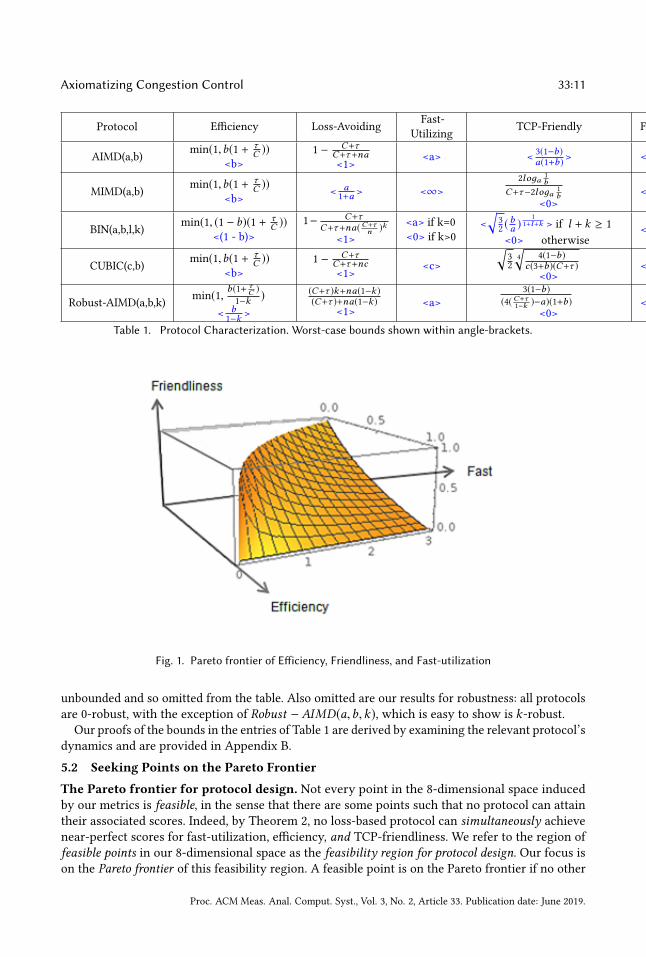
5.3 Experimental Validation

We validate our theoretical findings (shown in Table 1) via experiments with the Emulab network

emulator [48]. We stress that the purpose of our experimental investigation is not to show that the

achieved efficiency, convergence, friendliness, etc., exactly match the theoretical bounds in Table 1,

since differences would naturally arise from real-world aspects not captured by our theoretical

framework (such as timeouts). Nonetheless, we show how in spite of its simplifying assumptions, our

theoretical analysis successfully captures the trends produced by real-world interactions between

congestion control protocols.

Experimental framework. We experiment with the following protocols, implemented in the

Linux kernel: TCP Reno, TCP Cubic, and TCP Scalable. Our experiments investigated the interaction

of a varying number of connections (2-4) on a single link, for varying bandwidths (20Mbps, 30Mbps,



60Mbps, and 100Mbps), varying buffer sizes (10 MSS / 100 MSS), and a fixed RTT of 42ms. We

point out that each of the evaluated protocols represents a family of protocols formulated in

Section 2: Reno is AIMD(1,0.5), TCP Cubic is CUBIC(0.4,0.8), Scalable is MIMD(1.01,0.875) in some

environments and AIMD(1,0.875) in others (e.g., when RTT=42ms and the buffer size is 100MSS,

Scalable is AIMD for BW≤43.5Mbps andMIMD for bandwidth BW≥43.5Mbits/sec). Each experiment

lasted 2.5 minutes and iperf was used to measure the throughput attained by each sender at 0.5s

intervals.

Efficiency. To see how the trends in our theoretical results translate to real-world behavior, we

first consider the scenario with four senders where the buffer size is 10MSS and the bandwidth is

20Mbps. This, by the results in Table 1, induces a very clear hierarchy of protocols (from “worst”

to “best”): Reno (0.57), Cubic (0.91), Scalable (1.0). Fig 2(a) plots CDF of the efficiency observed

in our experiments, computed as the sum of rates for each sender averaged over 0.5s intervals,divided by the link bandwidth. A point (x ,y) in such a CDF captures the fraction of time-intervals

(y) over the entire experiment duration in which the efficiency was less than x .3 These experimental

results indeed reveal the exact same hierarchy over protocols. Figure 2(b) and (c) further show the

trends as we vary the buffer size and bandwidth respectively. Increasing the buffer size, keeping

the bandwidth fixed, increases theτC ratio, thus increasing efficiency value (given by b

(1 + τ

C

)). On

the other hand, increasing the bandwidth, keeping the buffer size fixed, decreases theτC ratio, thus

decreasing efficiency.

TCP-Friendliness. Table 2 presents a side-by-side comparison of the TCP-friendliness of the

examined protocols across multiple choices of number of senders n and link bandwidths BW for a

buffer of size 100MSS (see first row). Each experiment measured the average sending rate x̄ of n − 1

senders that employ the protocol under consideration, competing with a single TCP-Reno sender

on a single link. The level of TCP-friendliness was then set to bexRenox̄ , where xReno is the average

sending rate of the Reno sender. Our empirical results for TCP-friendliness present in Table 2

adhere to the theoretical lower-bound in Table 1. The theoretical lower-bound on α-friendlinessof Cubic in our setting is computed to be between 0.22 and 0.28. The empirical friendliness value

is between 0.28 and 0.72. The difference here primarily arises from a conservative estimate of

loss rate used in our worst-case theoretical analysis of Cubic friendliness. Observe, however that

in some of the empirical settings Cubic’s friendliness to TCP is very close to this lower-bound.

Scalable mostly behaves as AIMD(1,0.875) as its rate does not exceeds 44Mbps frequently, and so

according to Table 1 its TCP-friendliness level is close to 0.2, which is close to what we see in

our evaluated scenarios. Our results for other choices of buffer sizes are also consistent with the

theoretical results.

Our theoretical results for Robust-AIMD suggest that it constitutes a point in the design space

of congestion control protocols that provides performance comparable to AIMD in a significantly

more robust manner, while being more friendly to legacy TCP connections than PCC (whose

behavior is strictly more aggressive than MIMD(1.01,0.99)). In fact, the proof of our theoretical

result regarding the TCP-friendliness of Robust-AIMD shows that its TCP-friendliness is monotonein the number of Robust-AIMD connections, in the sense that the more Robust-AIMD connections

share a link the better its friendliness to TCP connections on the link becomes.

3Recall that α -efficiency of a protocol P means that from some point in time onwards any number of competing senders that

employ P will utilize at least an α -fraction of the link. Hence, even a protocol that achieves over 95% link utilization 99.999%

of the time but occasionally drops to 50% link-utilization is only formally1

2-efficient. Thus, the notion of α -efficiency, while

simple to reason about, is very sensitive to “noise”. Consequently, phenomena that are not modeled in our framework, such

as occasional transition to slow-start as a result of a timeout, can lead to very low efficiency according to our metric, even if

the protocol exhibits very high link-utilization in practice.


0.1 0.2 0.3 0.4 0.5 0.6 0.7 0.8 0.9 1.0Convergence

0.0

0.2

0.4

0.6

0.8

1.0

CD

F

reno cubic scalable

Fig. 3. CDF showing convergence for Reno, Cubic and Scalable TCP for four senders on 20Mbps link with abuffer of size10MSS.

(n,BW) (2,20 ) (2,30) (2,60) (2,100) (3,20) (3,30) (3,60) (3,100) (4,20) (4,30) (4,60) (4,100)R-AIMD / PCC 2.48x 1.69x 1.19x 1.94x 1.76x 1.35x 2.75x 1.92x 1.30x 2.47x 2.24x 2.00x

Table 3. TCP-friendliness of Robust-AIMD(1,0.8,0.01) vs. PCC

We experimentally evaluated Robust-AIMD(1,0.8, ϵ), for ϵ values of 0.005, 0.007, and 0.01 (cor-

responding to loss rates of 0.5%, 0.7%, and 1%, respectively). Representative experimental results

comparing Robust-AIMD’s TCP friendliness to PCC’s TCP friendliness appear in Table 3. Each

entry in the table specifies the improvement in % of Robust-AIMD(1,0.8) over PCC for different

choices of number of senders on the link (n) and link bandwidth, constant RTT of 42ms and buffer

size of 100 MSS. Observe that Robust-AIMD consistently attains >1.5x TCP-friendliness than PCC

(1.92x improvement on average).

Convergence. Our theoretical results in Table 1 establish the following ordering of protocols, in

terms of α-convergence (from “worst” to “best”): Reno (0.67), Cubic (0.89), Scalable (0.93). Figure 3

shows the CDF of convergence for our default scenario with four senders using a 20Mbps link with

buffer sized at 10MSS, generated as follows: Consider a sender i competing with other senders

over the bandwidth of a single link. Let s̄i denote the sender’s average rate over the entire durationof the experiment. A point (x ,y) in the plot captures the fraction (y) of 0.5s-long time-intervals

over the entire duration and across different senders, for which the convergence value was less

than x . Convergence value for a time-interval i was computed assis̄ifor si < s̄i and

(2 −

sis̄i

)for

si > s̄i , where si was the average rate in each interval. Thus, the CDF captures the distance of

a sender’s rate from the fixed rate s̄i , as defined in §3. Our experimental results reflect the same

general hierarchy of protocols as our theoretical results, with Reno’s convergence being smaller

than Cubic and Scalable and the last two having similar convergence behavior. We saw similar

trends in other experimental settings.

Fairness. As presented in Table 1 all evaluated protocols are, in theory, 1-fair (as Scalable behaves

like AIMD in the environments we tested). Our experimental results have been tabulated in Table 4.

Specifically, Table 4 (a) presents the results of experiments for n = 2 − 4 senders when all senders

start sending at the same time. Table 4 (b) presents results for the same experimental conditions,

but where one of senders starts 100s after others. We find that, for both cases, all protocols indeed

come fairly close to perfect fairness. Our results for other choices of parameters are also consistent

with the theoretical results.

Robustness. We now turn our attention to the robustness of protocols under different random

loss rates. Our theoretical result regarding the robustness of Robust-AIMD(1,0.8, ϵ) establishes that


(n,BW) (2,100) (3,100) (4,100)Reno 0.931 0.824 0.968

Cubic 0.858 0.878 0.926

Scalable 0.636 0.853 0.961

(a) All senders start at same time.

(n,BW) (2,100) (3,100) (4,100)Reno 0.921 0.898 0.952

Cubic 0.913 0.952 0.883

Scalable 0.944 0.911 0.967

(b) One sender starts late (after 100s)

Table 4. Fairness of Reno, Cubic and Scalable TCP for 100Mbps bandwidth and 100MSS buffers

0.003 0.005 0.007 0.01 0.05

Loss Rate

0.00.10.20.30.40.50.60.70.80.9

Link

Util

izat

ion

epsilon = 0.01 epsilon = 0.05

Fig. 4. Box-plots (with 5th, 25th, 50th, 75th, and 95th percentile values) comparing robustness of Robust-AIMDfor ϵ = 0.01 and ϵ = 0.05

the higher the value of ϵ the more robust the protocol is. We experimentally evaluated Robust-

AIMD(1,0.8, ϵ), for ϵ values of 0.01 and 0.05 (corresponding to loss rates of 1% and 5%, respectively).

Fig. 4 presents box plots of link utilization (sending rate divided by the bandwidth) for a single

sender using a link of capacity 100Mbps with buffer size 100MSS under varying loss rates. Our

experimental results reflect the expected hierarchy over Robust-AIMD protocols: the sender with

the higher ϵ = 0.05 is more robust than the sender with ϵ = 0.01, with the difference between the

two decreasing as the loss rate is increased. Our results for other choices of parameters are also

consistent with the theoretical results.

6 High Throughput or Low Latency/Loss? Pick!As shown in Section 4 and in Section 5, the simple fluid-flow model of dynamics of congestion

control protocols presented in Section 2 enables reasoning about fundamental tradeoffs in protocol

design that, we believe, extend well beyond the scope of the model. However, the limitations of

this simplified model render it impossible to reason about some other fundamental tradeoffs. We

thus extend this model to establish another fundamental tradeoff—between the desideratum of

achieving high (average) throughput and the desideratum of maintaining low (average) latency/loss

in unpredictable and dynamic environments.

Wireless networks have been the subject of much attention as the unpredictability and variability

of available bandwidth in such networks make them particularly challenging from a protocol design

perspective. The experimental results of recent studies (see Figures 9 and 10 in [50] and Figure 6

in [19]) suggest that simultaneously attaining high throughput and keeping latency low in such

environments is impossible, and that different protocols reflect different tradeoffs between these

two desiderata. We show how this can be formalized and proved within our axiomatic framework.


6.1 Revisiting Our Model and Axioms

Revised model. We change the model of Section 2 as follows. Now, the link’s bandwidth can

change every RTT. Each sender must select a rate for time step t at the beginning of the time step

and without knowledge of the bandwidth of the link B(t )at that time step. We assume that for

all t , B1 ≤ B(t ) ≤ B2 for some fixed values B1 and B2. Let the capacity C(t )of the link at time t

be C(t ) = B(t ) × 2Θ (recall that Θ is the link’s propagation delay). All other aspects of the model

remain as in Section 2. We show below that well-utilizing the link in this model is at odds with

maintaining low latency and loss even if only a single sender is using the link. Hence, to simplify

exposition, let us focus henceforth on the single-sender scenario. Our theoretical results below

easily extend to multiple senders.

We note that the above extension to our model is inspired by the experimental framework for

evaluating congestion control protocols on LTE networks used in [19, 50] (using Mahimahi [34] on

Verizon-LTE traces).

Revised axioms. To reason about the tradeoffs between different desiderata, we revisit the ef-

ficiency, loss-avoidance, and latency-avoidance axioms from Section 3 (Metrics I, III, and VIII,

respectively), and adapt the formulation of these axioms to the above extended model. Specifically,

the new formulations of the axioms capture not only eventual behavior (“from some time onwards”)

but also temporal aspects of congestion control protocols (how well the protocol behaves within a

certain time frame).

The new formulation of the efficiency axiom quantifies how close the average utilization of the

link within a time frame is to the maximum volume of traffic the link could have carried during

that time. This enables us to reason about the average link utilization over time. As the link’s RTT

can vary over time, the efficiency axiom formulation averages over link utilization at different time

steps proportionally to the RTTs of these time steps.

Efficiency. We say that a congestion-control protocol P is α-efficient if when the sender employs

P , then for any time T ,

ΣTt=1RTT (t) × min(X (t ),C (t ))

C (t )

ΣTt=1RTT (t)

≥ α

Our next two axioms bound the average per-packet loss rate and latency.

Loss-avoidance.We say that a congestion-control protocol P is α -loss-avoiding if when the sender

employs P , then for any time T ,

ΣTt=1X (t ) × L(t )

ΣTt=1X (t )

≤ α .

Latency-avoidance. We say that a congestion-control protocol P is α-latency-avoiding if when

the sender employs P , then for any time T , for sufficiently large buffer size τ ,

ΣTt=1X (t ) × RTT (t)

ΣTt=1X (t )

< (1 + α)2Θ.

6.2 Throughtput vs. Latency

Suppose, for now, that the buffer is of infinite size so as to remove packet loss from consideration and

focus solely on the implications of rate choices for latency. As discussed next, intuitively, attaining

high throughput and maintaining low latency in this setting cannot be accomplished simultaneously.

Clearly, the sender can simply bombard the link with traffic so as to achieve consistently high

throughput at the cost of high latency. Alternatively, the sender can send at very low rates to

attain perfect latency at the cost of low average bandwidth utilization. Can congestion control

protocols achieve both desiderata simultaneously? Our next two results show that the answer to

this question is negative. This sheds light on the recent experimental findings in [19, 50] for LTE

networks (see Figures 9 and 10 in [50] and Figure 6 in [19]), which experimentally demonstrate the

tradeoff between the two desiderata.

Observe that the protocol that leaves the congestion window fixed at 2θB1 (the minimum possible

bandwidth of the link) is triviallyB1

B2

-efficient (as the maximum link bandwidth is B2) and minimizes

latency (i.e., is 0-latency avoiding). We show next that any improvement in efficiency over this

simple protocol comes at the cost of worse latency, where the higher the improvement in efficiency

is the worse the resulting latency is.

Theorem 7. Any protocol that isα -efficient forα > B1

B2

is notB1(B2−B1)+(γ−(γ )2)B2

2−2B2

√(1−γ )γ B1(B2−B1)

((1−γ )B2−B1)2

-latency-avoiding for any γ < α .

We next present the “converse” of Theorem 7, which shows that maintaining low latency must

come at the cost of suboptimal bandwidth utilization.

Theorem 8. Any protocol that isα -latency avoiding forα > 0, is not(γ+1)(B2−B1)+2B1−B2+2

√B1(B2−B1)γ

B2(γ+1)

-efficient for any γ > α .

We now provide a sketch of the proof of Theorem 7. The proofs of the other theorems of this

section employ a similar methodology.

Proof sketch for Theorem 7. To provide the intuition for the proof and simplify exposition,

consider the following setting: The single sender participates in a game against an adversary; at

the beginning of each time step t , the sender sets the size of its congestion window and then the

adversary selects the bandwidth B(t )for that time step. We will show that link bandwidths can be

selected in a manner that induces average latency of at least

2θB2

((1−α )(B2−B1)+αB1−2

√(1−α )αB1(B2−B1)

)((1−α )B2−B1)

2,

yielding the bound in the statement of the theorem. While this setting reflects a view of the

environment as “hostile” and capable of adapting the link’s bandwidth in response to the sender’s

actions, the bound of Theorem 7 can be established even in model where the link’s bandwidth at

each point in time is drawn from a fixed probability distribution over B1 and B2 that is constant

across time (and so the environment is completely oblivious to the sender’s choices of rates and

exhibits stochastic regularity). We later discuss how the proof methodology presented below (for

the adversarial setting) can be extended to the stochastic setting.

Consider the following strategy for the adversary: Choose a fixed “threshold”B1

B2

< β < α . When

the sender’s chosen window size is at most βB2 × 2Θ, set B2 as the link bandwidth for that time

step. When the sender’s chosen window size is above βB2 × 2Θ, set B1 as the link bandwidth for

that time step.

What should the sender do against this adversarial strategy? Observe that as the link’s bandwidth

is always within the interval [B1,B2], the sender cannot gain anything, in terms of performance,

from choosing a congestion window of size below B1 × 2Θ or above B2 × 2Θ. In fact, the following

is easy to show.

Claim 2. The sender’s optimal strategy always selects congestion window sizes within the interval[βB2 × 2Θ, (β + ϵ)B2 × 2Θ] for an arbitrarily small choice of ϵ > 0.

To see this, consider first the scenario that the sender’s congestion window is strictly beneath

βB2 × 2Θ. Then, as in this scenario the realized bandwidth is B2, a congestion window of size

βB2 × 2Θ would have led to the exact same realized link bandwidth, but would have resulted in

strictly better link utilization (and the same latency). Now, consider the scenario that the sender’s

congestion window is strictly above (β + ϵ)B2 × 2Θ. Then, as in this scenario the realized link

bandwidth is B1, a congestion window of size precisely (β + ϵ)B2 × 2Θ would have led to the exact

same realized link bandwidth, but would have resulted in strictly better latency (and the same

link utilization, i.e., 100%). Claim 2 implies that the sender’s best strategy is effectively constantly

sending at a rate of βB2 × 2Θ, and its decisions effectively boil down to whether the congestion

window should be of size precisely βB2 × 2Θ, which we will refer to as deciding “DOWN”, or the

congestion window size should be slightly above βB2 × 2Θ, which we will refer to as deciding “UP”.

Given the adversary’s strategy, every time UP is decided the realized link bandwidth is B1 and

every time DOWN is decided the realized bandwidth is B2.

Since the sender is α-efficient on average, no matter what the link bandwidths are, at least an

α-fraction of the link must be utilized on average. This implies that the sender cannot decide

DOWN “too often” as this will result in “too many” time steps in which the sender’s window size is

βB2 × 2Θ but the link capacity is B2 × 2Θ and, as β < α , the link utilization is “low”. The following

claim formalizes this intuition.

Claim 3. For any 0 < α < 1 and B1

B2

< β < α , the sender’s optimal strategy cannot decide DOWN

in more than a (1−α )βB2

(1−α )βB2+(α−β )B1

-fraction of the time steps.

This, of course, implies that the sender’s optimal strategy must decide UP in at least (in fact,

precisely) a(α−β )B1

(1−α )βB2+(α−β )B1

-fraction of the time steps. Since every time UP is decided, the realized

bandwidth is B1, this implies that in(α−β )B1

(1−α )βB2+(α−β )B1

-fraction of the time steps, the sender sends

at a rate that is higher than the bandwidth and so suffers from increased latency. Specifically, at

each such time step t more than βB2 × 2Θ packets are sent, and so the latency for that time step

RTT (t) is at least 2θ × (1 +βB2−B1

B1

). Even assuming that in all other time steps the latency is 2Θ

(the minimum), this results in average latency of2θ (1−β )βB2

(α−β )B1+β (1−α )B2

.

Given the sender’s optimal strategy with respect to a value β , as discussed above, the adversary

can compute the value of β that maximizes the sender’s average latency. Our calculations show

that the resulting average latency value cannot be within a multiplicative factor of

1 +

[B1(B2 − B1) +

(α − α2

)B2

2− 2B2

√(1 − α)αB1(B2 − B1)

((1 − α)B2 − B1)2

]of the minimum latency (2Θ). As the above formula is monotone increasing in α for α ∈ [

B1

B2

, 1],

this yields the bound of Theorem 7.

While the proof sketch above considers an adversarial environment, the bound of Theorem 7

applies also when the link’s bandwidth is B1 with probability p and B2 with probability 1 − p for a

fixed probability p that is constant over time. Extending our proof technique to this context involves

setting p =(α−β )B1

(1−α )βB2+(α−β )B1

(i.e., precisely the fraction of time presented in Claim 3). Then, the

arguments above can be adapted to show that the sender’s optimal strategy is setting the congestion

window size to be precisely βB2 ×2Θ, leading to the same lower bound on latency. More specifically,

our proof shows that under this probability distribution over link bandwidth, the sender’s optimal

strategy is constantly setting its window size to βB2 × 2Θ. The calculation of the average latency

resulting from this choice of congestion window yields the bound of Theorem 7.

6.3 Throughput vs. Loss

As the next two results show, when the buffer size is finite, the desideratum of attaining high

throughput and the desideratum of keeping (average) loss rate low are also at odds.

Theorem 9. Any protocol that is α-efficient for α > B1

B2

is not(2−γ )B2−B1−2

√(1−γ )B2(B2−B1)

γ B2

-lossavoiding, for all γ < α .

Theorem 10. Any protocol that isα -latency avoiding forα > 0, is not2

√γ (B2−B1)(B1+B2γ )−B1γ+B1+2B2γ

B2(γ+1)2-

efficient for all γ > α .

7 Related WorkThe axiomatic approach. The axiomatic approach is deeply rooted in the theory of social choice,

whose focus is on how to combine individual opinions into collective decisions. Classical ap-

plications include Arrow’s celebrated Impossibility Theorem [7] and the Gibbard-Satterthwaite

Theorem [22, 41].

The axiomatic approach has also been applied to many computer science environments, including

ranking systems [2, 3], reputation systems [47], recommendation systems [6], routing protocols [28],

link prediction [17], sustainable developments [15], and relating ACK-clocking and actual data-

flow rate [12]. We are, to the best of our knowledge, the first to apply the axiomatic approach to

congestion control protocols.

Network-utility maximization (NUM). NUM is a prominent framework for analyzing and

designing TCP protocols, pioneered by Kelly et al. [26]. [33] shows how a simple formulation of

a convex program for maximizing the “social welfare” of senders of traffic across a network can

be used to derive both congestion control policies for the end-hosts and queueing policies for

in-network devices (routers) via the primal dual schema. NUM is useful for both (1) gaining insights

into existing (TCP) protocols (by reverse engineering the implicit utility functions being optimized)

and (2) designing new TCP protocols (by building into the protocol the desired utility function)

with respect to specific, perdetermined objectives (captured by connections’ utility functions). Our

focus, in contrast, is on outlining the possibility/impossibility borderline for congestion control by

studying the delicate interplay between different desired properties.

Control-theoretic approaches to TCP congestion control. Control theory has been applied

to reason about the implications of rate modulation by a specific protocol for performance, stability,

and fairness [43], with respect to different active queue management schemes [25, 38], buffer sizes

[39], network topologies and traffic patterns, etc. As discussed above, our focus is on the inherent

limitations for congestion control protocol design.

Analyzing TCP dynamics. Our model for reasoning about dynamics of congestion control builds

upon classical models for analyzing TCP dynamics [9, 13, 16, 30, 35, 36, 40].

8 ConclusionWe have put forth an axiomatic approach for analyzing congestion control designs, which comple-

ments the current simulation/experimentation and theoretical approaches. Our approach uses a

simple model, and a set of axioms, to gain insight into which properties can co-exist, and which

follow from other properties. Our results characterize a Pareto frontier for congestion control that

defines the borderline between possibility and impossibility. While derived in the context of a

simple model, these results shed light on past empirical and experimental findings and provide

guidance for future design efforts. We view our results as a first step and leave the reader with

many research directions relating to the extension of our model and the re-examination of our

axioms/metrics (Section 3). Thus far, axiomatic approaches have been applied to a few, very spe-

cific, networking environments [17, 28, 42]. We believe that applying the axiomatic approach to

other networking contexts (e.g., intradomain [28] and interdomain routing, traffic engineering,


in-network queueing [45], network security) could contribute to more principled discussions about

these contexts.

References[1] M. Alizadeh, A. Kabbani, B. Atikoglu, and B. Prabhakar. Stability analysis of QCN: the averaging principle. In

SIGMETRICS, 2011.[2] A. Altman and M. Tennenholtz. Axiomatic foundations for ranking systems. Journal of Artificial Intelligence Research,

2008.

[3] A. Altman and M. Tennenholtz. An axiomatic approach to personalized ranking systems. Journal of the ACM (JACM),2010.

[4] E. Altman, K. Avrachenkov, and B. Prabhu. Fairness in MIMD congestion control algorithms. In INFOCOM 2005, 2005.[5] E. Altman, R. El-Azouzi, Y. Hayel, and H. Tembine. The evolution of transport protocols: An evolutionary game

perspective. Computer Networks, 2009.[6] R. Andersen, C. Borgs, J. Chayes, U. Feige, A. Flaxman, A. Kalai, V. Mirrokni, and M. Tennenholtz. Trust-based

recommendation systems: an axiomatic approach. In World Wide Web, 2008.[7] K. J. Arrow. A difficulty in the concept of social welfare. Journal of political economy, 1950.[8] V. Arun and H. Balakrishnan. Copa: Practical delay-based congestion control for the internet. In 15th USENIX

Symposium on Networked Systems Design and Implementation (NSDI 18), pages 329–342, Renton, WA, 2018.

[9] D. Bansal and H. Balakrishnan. Binomial congestion control algorithms. In INFOCOM, 2001.

[10] B. Braden, D. Clark, J. Crowcroft, B. Davie, S. Deering, D. Estrin, S. Floyd, V. Jacobson, G. Minshall, C. Partridge, et al.

Recommendations on queue management and congestion avoidance in the internet. Technical report, 1998.

[11] L. S. Brakmo and L. L. Peterson. TCP vegas: End to end congestion avoidance on a global internet. IEEE Journal onselected Areas in communications, 1995.

[12] Briat, Hjalmarsson, Johansson, Jonsson, Karlsson, Sandberg, and Yavuz. An axiomatic fluid-flow model for congestion

control analysis. In Decision and Control and European Control Conference (CDC-ECC), 2011 50th IEEE Conference on,pages 3122–3129. IEEE, 2011.

[13] L. Cai, X. Shen, J. Pan, and J. W. Mark. Performance analysis of TCP-friendly AIMD algorithms for multimedia

applications. Transactions on Multimedia, 2005.[14] N. Cardwell, Y. Cheng, C. S. Gunn, S. H. Yeganeh, and V. Jacobson. BBR: Congestion-based congestion control. Queue,

2016.

[15] G. Chichilnisky. An axiomatic approach to sustainable development. Social choice and welfare, 1996.[16] D.-M. Chiu and R. Jain. Analysis of the increase and decrease algorithms for congestion avoidance in computer

networks. Computer Networks and ISDN systems, 1989.[17] S. Cohen and A. Zohar. An axiomatic approach to link prediction. In AAAI. Citeseer, 2015.[18] M. Dong, Q. Li, D. Zarchy, P. B. Godfrey, and M. Schapira. PCC: Re-architecting congestion control for consistent high

performance. In NSDI 15, 2015.[19] M. Dong, T. Meng, D. Zarchy, E. Arslan, Y. Gilad, B. Godfrey, and M. Schapira. Vivace: Online-learning congestion

control. In 15th USENIX Symposium on NSDI 18. USENIX Association, 2018.

[20] S. Floyd. Metrics for the Evaluation of Congestion Control Mechanisms. RFC 5166, Mar. 2008.

[21] S. Floyd, M. Handley, and J. Padhye. A comparison of equation-based and AIMD congestion control. 2000.

[22] A. Gibbard et al. Manipulation of voting schemes: a general result. Econometrica, 1973.[23] P. Godfrey, M. Schapira, A. Zohar, and S. Shenker. Incentive compatibility and dynamics of congestion control. In

SIGMETRICS, 2010.[24] S. Ha, I. Rhee, and L. Xu. CUBIC: a new TCP-friendly high-speed TCP variant. ACM SIGOPS Operating Systems Review,

2008.

[25] C. V. Hollot, V. Misra, D. Towsley, and W.-B. Gong. On designing improved controllers for aqm routers supporting

tcp flows. In INFOCOM 2001. Twentieth Annual Joint Conference of the IEEE Computer and Communications Societies.Proceedings. IEEE, volume 3, pages 1726–1734. IEEE, 2001.

[26] F. P. Kelly, L. Massoulié, and N. S. Walton. Resource pooling in congested networks: proportional fairness and product

form. Queueing Systems, 63(1):165, 2009.[27] T. Lakshman and U. Madhow. The performance of TCP/IP for networks with high bandwidth-delay products and

random loss. Transactions on Networking (ToN), 1997.[28] O. Lev, M. Tennenholtz, and A. Zohar. An axiomatic approach to routing. In INFOCOM 2015, 2015.[29] Y. Liu and W. Gong. On fluid queueing systems with strict priority. IEEE Transactions on Automatic Control, 2003.[30] M. Mathis, J. Semke, J. Mahdavi, and T. Ott. The macroscopic behavior of the TCP congestion avoidance algorithm.

SIGCOMM, 1997.



[31] R. Mittal, N. Dukkipati, E. Blem, H. Wassel, M. Ghobadi, A. Vahdat, Y. Wang, D. Wetherall, D. Zats, et al. TIMELY:

RTT-based congestion control for the datacenter. In SIGCOMM, 2015.

[32] J. Mo, R. J. La, V. Anantharam, and J. Walrand. Analysis and comparison of TCP reno and vegas. In INFOCOM’99, 1999.[33] J. Mo and J. Walrand. Fair end-to-end window-based congestion control. IEEE/ACM Transactions on Networking (ToN),

2000.

[34] R. Netravali, A. Sivaraman, S. Das, A. Goyal, K. Winstein, J. Mickens, and H. Balakrishnan. Mahimahi: Accurate

record-and-replay for HTTP. In 2015 USENIX Annual Technical Conference (USENIX ATC 15), 2015.[35] T. Ott, J. Kemperman, and M. Mathis. The stationary behavior of ideal TCP congestion avoidance. 1996.

[36] J. Padhye, V. Firoiu, D. Towsley, and J. Kurose. Modeling TCP throughput: A simple model and its empirical validation.

SIGCOMM, 1998.

[37] F. Paganini, J. Doyle, and S. H. Low. A control theoretical look at internet congestion control. Lecture notes in controland information sciences, 2003.

[38] P.-F. Quet and H. Ozbay. On the design of aqm supporting tcp flows using robust control theory. IEEE transactions onautomatic control, 49(6):1031–1036, 2004.

[39] G. Raina, D. Towsley, and D.Wischik. Part ii: Control theory for buffer sizing. ACM SIGCOMMComputer CommunicationReview, 35(3):79–82, 2005.

[40] R. Rejaie, M. Handley, and D. Estrin. RAP: An end-to-end rate-based congestion control mechanism for realtime

streams in the internet. In INFOCOM’99, 1999.[41] M. A. Satterthwaite. Strategy-proofness and arrow’s conditions: Existence and correspondence theorems for voting

procedures and social welfare functions. Journal of economic theory, 1975.[42] S. Shenker. A theoretical analysis of feedback flow control. In SIGCOMM, 1990.

[43] R. Shorten, F. Wirth, and D. Leith. A positive systems model of TCP-like congestion control: asymptotic results.

Transactions on Networking (TON), 2006.[44] M. Shreedhar and G. Varghese. Efficient fair queuing using deficit round-robin. Transactions on networking, 1996.[45] A. Sivaraman, K. Winstein, S. Subramanian, and H. Balakrishnan. No Silver Bullet: Extending SDN to the Data Plane.

In Twelfth ACM Workshop on Hot Topics in Networks (HotNets-XII), College Park, MD, November 2013.

[46] R. Srikant. The mathematics of Internet congestion control. 2012.[47] M. Tennenholtz. Reputation systems: An axiomatic approach. In Uncertainty in artificial intelligence, 2004.[48] B. White, J. Lepreau, L. Stoller, R. Ricci, S. Guruprasad, M. Newbold, M. Hibler, C. Barb, and A. Joglekar. An integrated

experimental environment for distributed systems and networks. In USENIX OSDI, 2002.[49] K. Winstein and H. Balakrishnan. TCP ex machina: Computer-generated congestion control. In SIGCOMM, 2013.

[50] K. Winstein, A. Sivaraman, H. Balakrishnan, et al. Stochastic forecasts achieve high throughput and low delay over

cellular networks. In NSDI, 2013.[51] F. Wirth, R. Stanojević, R. Shorten, and D. Leith. Stochastic equilibria of AIMD communication networks. SIAM Journal

on Matrix Analysis and Applications, 2006.[52] Y. R. Yang and S. S. Lam. General AIMD congestion control. In Network Protocols, 2000, 2000.[53] L. Zhang, S. Shenker, and D. D. Clark. Observations on the dynamics of a congestion control algorithm: The effects of

two-way traffic. SIGCOMM, 1991.

A Axiomatic Derivation Proofs (Section 4)Proof of Theorem 2: Let P be loss based, α-fast-utilizing and β-efficient protocol. We next show

that P is no more TCP-friendly than AIMD(α , β). Consider first the case of two senders, namely a

single P-sender and a single TCP-sender.

• α-fast-utilization implies that any P-sender, on average, additively increase its window size

by at least α MSS per RTT so long as no packet loss occurs.

• The link-utilization requirement (Metric I) and Lemma 12 (in §A.1), imply that the P sender

does not decrease its window size by a multiplicative factor larger than β upon encountering

loss.

Combined, this implies that the time duration between two consecutive loss events when competing

with TCP Reno (i.e., AIMD(1, 1

2)) on a link is no higher than the time duration between two

consecutive loss events when AIMD(α , β) competes with TCP Reno on the same link. The above

arguments can be generalized to anym1 TCP senders competing withm2 P-senders on a bottleneck

link. Now, the sum of window sizes of all senders additively increases by at leastm1 +m2α when



no loss occurs, and decreases by no more than β when loss does occur. Using arguments similar

to those above, we get that the TCP-friendliness of P is no higher than the TCP-friendliness of

AIMD(α , β).

To complete the proof, we show that AIMD(α , β) is3(1−β )α (1+β ) friendly. Suppose that there arem1

TCP senders, andm2 P-senders. W.l.o.g., we can treat them1 TCP-senders as a single AIMD(m1,1

2)

sender (denoted by T ∗), and them2 AIMD(α , β) senders as a single AIMD(αm2, β) sender (denoted

by P∗). By Lemma 11, the TCP window size when competing against (α , β)-AIMD, when the link is

fully utilized is

x∗TCP =1

m1

T ∗ =1

m1

(2m1(1 − β)(C + τ )

2m1(1 − β) + αm2

)(6)

Once packet loss occurs, the window size of each TCP sender is decreased to 0.5(x∗TCP ) (whereafter sufficiently long time all TCP senders have equal window size [16]). Hence, the average

window size of each TCP sender is x̄TCP =1+0.5

2x∗TCP . This yields

x̄TCP =3(1 − β)(C + τ )

4m1(1 − β) + 2αm2

(7)

By Lemma 11, the window size of each P-sender when the link is fully utilized is

x∗P =1

m2

P∗ =1

m2

(αm2(C + τ )

2m1(1 − β) + αm2

)(8)

Upon experiencing loss, the window size of any P-sender is β(x∗P ). Hence, the average window size

of a P-sender is x̄P =1+β

2x∗P . This yields

x̄P =α(1 + β)(C + τ )

4m1(1 − β) + 2αm2

(9)

Sincex̄TCPx̄P=

3(1−β )α (1+β ) , P is at most

3(1−β )α (1+β ) -TCP friendly.

Proof of Theorem 3: Let P be a loss based, α-fast-utilizing, β-efficient, and ϵ-robust protocol. Ar-guments similar to those in the proof of Theorem 2 imply that to upper bound P ’s TCP-friendliness,it is sufficient to upper bound the TCP-friendliness of Robust-AIMD(α , β, ϵ). We hence restrict our

attention hereafter to upper bounding the TCP-friendliness of Robust-AIMD(α , β, ϵ).Consider first, to simplify exposition, the following 2-sender setting. Let p1 be a TCP sender

(i.e., AIMD(1, 0.5)) and p2 be a Robust-AIMD(α , β, ϵ) sender that competes with p1 on the link. To

analyze the dynamics of the two senders, we consider three possible scenarios for any given point

in time t :

(1) Scenario I: No loss event occurs.

(2) Scenario II: Loss occurs, but the loss rate is at most ϵ .(3) Scenario III: The loss rate is higher than ϵ .

In the first scenario, both senders increase their window sizes (p1 by MSS and p2 by α MSS). In the

second scenario, the two senders react in an opposite manner: p2 additively increases its window

size by α MSS per RTT, while p1 halves its window size. In the third scenario, both senders decrease

their window sizes (p1 halves its window size and p2 decreases its window size by a multiplicative

factor of β).To upper bound the friendliness, we consider the scenario that the link capacity C»αMSS and

the buffer size is dominated by the link capacity (i.e.,C >> τ ). We make the following observations

about how dynamics transition between the three scenarios.



• When in scenario I, the two senders will gradually increase their window sizes until, at some

later point in time, reaching Scenario II. We denote this by I → I I .• When in scenario II, the two senders will adjust the sending rates in opposite directions,

reaching either Scenario I (if p1’s change to its congestion window dominates p2’s) or Scenario

III (otherwise).

• When in Scenario III, both senders will decrease their sending rates, eventually reaching

Scenario I.

Thus, any dynamics of interaction between the two senders is expected to result in a sequence of

transitions between scenarios of the form I → I I → I → I I → . . .→ I → I I → I I I → I → I I →I → I I → . . .→ I → I I → I I I → I → . . .. An illustration of such dynamics is presented in Fig. 5.

We call a subsequence connecting every two appearances of Scenario III a “cycle”. To determine the

TCP-friendliness of p2, we compute the average window size of p1 and p2 over the course of a cycle

and examine the ratio between them. We refer to a transition of the form I → I I as a sub-cycle.We observe that in any subsequence of the form I → I I → . . .→ I → I I → I . . ., p2 constantly

increases its window size and, moreover, Scenario III will be reached only once the window size of

p1 is below 2αMSS (for only then, halving p1’s window size in Scenario II is dominated by increasing

p2’s window size by αMSS. Thus, whenever Scenario I is realized, the sending rates will eventually

be so that p2 completely dominates the link and p1 is effectively sends at a rate of almost 0 (as

αMSS«C). Once this happens, p2 will keep increasing its rate until Scenario III is realized, and so

on.

Immediately after reaching Scenario III, the window size of p2 is βC+τ1−ϵ (Lemma 14), while p1’s

window size remains effectively 0.

Consider a specific cycle, and let S i denote the i’th sub-cycle in S . Let xLi and xHi denote the

smallest window size and the largest window size of p1 in S i , respectively, and let yLi and yHi

denote the smallest window size and the largest window size of p2 in Si, respectively. Let Ti denote

the duration of sub-cycle S i . Note that Ti = xHi − xLi (as the additive increase for TCP Reno is 1).

Building on the above observations, we now broaden our focus to the more general setting in

whichm1 p1-senders compete withm2 p2-senders. Using the same argument as in the proof of

Theorem 2, them1 p1-senders can be regarded as a single AIMD(m1,1

2)-sender, denoted by P1, and

them2 p2-senders can be regarded as a single Robust-AIMD(m2α ,b, ϵ)-sender, denoted by P2. As in

the 2-sender analysis, in every sequence of sub-cycles, P2 increases its window size until it entirely

dominates the link capacity. Hence, the duration of a cycle is T =(1−β )(C+τ )m2α (1−ϵ )

. Consequently, the

average window size of P1 in one cycle is:

1

T

( xH1∑

x t=L1

x t + ... +

xHN∑x t=LN

x t

)=

m2αC+τ1−ϵ (1 − β)

N∑i=1

(xLi + xHi )

2

(xHi − xLi )

=m2α

2C+τ1−ϵ (1 − β)

N∑i=1

(x2

Hi−x2

Hi−1

4

) (10)

where the last equality follows from P1 halving its window size (that is, xLi =xHi−1

2). We next

compute xLi and xHi . In the beginning of cycle, P1’s window size is (effectively) 0, and so xL0= 0,

and P2 starts at βC+τ1−ϵ . In the beginning of each sub-cycle S

i, (C+τ −(xLi−1

+yLi−1)) is left to consume


before the cycle ends, and the sum of the window increases of the two senders ism1 +m2α . Thus,

each sub-cycle lasts Ti =C+τ−(xLi−1

+yLi−1)

m1+m2αtime steps.

In addition, note that

xHi = xLi +C + τ − (xLi + yLi )

m1 +m2α(11)

Since xLi =xHi−1

2, and as P2 grows bym2αMSS each RTT, yLi = yHi−1

+m2α , we have that

Ti =C + τ − (

xHi−1

2+ yHi−1

+m2α)

m1 +m2α≈C + τ − (

xHi−1

2+ yHi−1

)

m1 +m2α

where the last step holds true asm2α

m2α+m1

< 1. To determine xHi , we write the recurrence relation

for xHi and yHi to describe how they progress.

xHi =xHi−1

2

+m1

[C + τ − (

xHi−1

2+ yHi−1

)

m1 +m2α

](12)

yHi = yHi−1+m2α

[C + τ − (

xHi−1

2+ yHi−1

)

m1 +m2α

](13)

After some algebraic manipulation of (12) and (13), we isolate a recurrence relation for xHi only,

xHi = xHi−1

2m1 +m2α

2(m1 +m2α)(14)

Solving (14) using initial condition xH1=

C+τ1−ϵ (1−β−ϵ )m1

m2α+m1

<C+τ1−ϵ (1−β )m1

m2α+m1

(which is derived from the

time it takes to fully utilize the bandwidth) gives an upper bound of xHi as a function of i ,

xHi =2(1 − ϵ − β)C+τ

1−ϵ

2m1 +m2α

(m2α + 2m1

2(m1 +m2α)

) i(15)

<2(1 − β)C+τ

1−ϵ

2m1 +m2α

(m2α + 2m1

2(m1 +m2α)

) i(16)

Plugging (15) in (10), assigning a total time of T =(1−β )(C+τ )m2α (1−ϵ )

, and replacing N with ∞ (after N

sub-cycles HN − LN is effectively zero, as the link is almost utilized and the p1 sender sends at most

1 MSS), we get that the average window size of P1 is at most,

m2α

2C+τ1−ϵ (1 − β)

(C+τ1−ϵ (1 − β)m1

m1 +m2α

)2

+

∞∑i=2

(C+τ1−ϵ (1 − β)2m1

2m1 +m2α

(2m1 +m2α

2(m1 +m2α)

) i )2

−1

4

∞∑i=2

(C+τ1−ϵ (1 − β)2m1

2m1 +m2α

(2m1 +m2α

2(m1 +m2α)

) i−1

)2

=

C+τ1−ϵ (1 − β)3m1

2(3m2α + 4m1)(17)


On the other hand, since P2 starts to increase its window size at β C+τ1−ϵ until its window size is

C+τ1−ϵ (with a window size increase ofm2α at each step), the average window size of P2 in a single

sub-cycle is,

C+τ1−ϵ (1 + β)

2

(18)

Since multiple AIMD senders converge to a fair rate configuration amongst themselves [16], and

this is also true for Robust-AIMD senders (using the same analysis), to quantify the TCP-friendliness

of Robust-AIMD(α , β , ϵ), we need to compute the ratio R between the average window size of any

p1-sender (using (17)) and the average window size of any p2-sender (18)). This boils down to at

most

R =

1

m1

·C+τ1−ϵ (1−β )3m1

2(3m2α+4m1)

1

m2

·C+τ1−ϵ (1+β )

2

=3m2(1 − β)

(3m2α + 4m1)(1 + β)(19)

In particular, by Equation (19), the ratio for a single Robust-AIMD(1, 1

2, ϵ) sender and a single TCP

Reno sender is R =3·(1− 1

2)

(3+4)(1+ 1

2)= 1

7. Note that the ratio R increases with the number of robust-AIMD

senders and decreases with the number of TCP senders, so long as the congestion loss is no larger

than ϵ (as otherwise all senders decrease their window size). Hence, the worst-case value for

TCP-friendliness is achieved whenm2 = 1 andm1 satisfies

m1 + 1 · α =C + τ

1 − ϵ(20)

where (20) bounds the number of TCP senders given that each sender’s window size is 1 MSS. From

(20) it follows that the lowest ratio R is obtained when

m1 =C + τ

1 − ϵ− α (21)

Plugging expression (21) into (19) and rearranging the terms yields

R =3(1 − β)

(4(C+τ1−ϵ ) − α)(1 + β)

Hence, any ϵ-robust AIMD is at most3(1−β )

(4(C+τ1−ϵ )−α )(1+β )

-friendly.

Fig. 5. Dynamics of TCP vs. Robust-AIMD(1,0.5,0.01). The figure plots the windows sizes across time. Thelink’s bandwidth-delay product is 800 MSS and a buffer size is 200 MSS. The Robust-AIMD sender increasesits window size until its experienced loss rate is 0.01.


Proof of Theorem 4:When ϵ << β , the value of xHi in the proof of Theorem 3 becomes:

xHi =2(1 − ϵ − β)C+τ

1−ϵ

2m1 +m2α

(m2α + 2m1

2(m1 +m2α)

) i≈

2(1 − β)C+τ1−ϵ

2m1 +m2α

(m2α + 2m1

2(m1 +m2α)

) i(22)

The proof of Theorem 4 then follows directly from the proof of Theorem 3.

Proof of Theorem 5: Let x̄P and x̄TCP be the average window sizes of P and TCP, respectively,

when competing against each other on the link. Suppose that P is α-TCP-friendly. Then, α · x̄P <x̄TCP . Let x̄Q and x̄ ′TCP be the average window size of Q and TCP respectively when they compete

each other on the same link. Suppose that Q is more aggressive to TCP. Then x̄ ′TCP < x̄Q .Bansal and Balakrishnan [9] showed that given a loss frequency p (the ratio between the number

of time steps in which loss occurs and the overall number of time steps), any protocol of type

BIN(a,b, l ,k) converges to an average window size that is proportional to,(a

(1 − b)p

) 1

l+k+1

(23)

for any l ≤ 1,k ≥ −1. Let Ma,b,l,k (p) denote(

a(1−b)p

) 1

l+k+1

where a,b, l ,k are the corresponding

parameters for protocol M. Since αx̄P < x̄TCP (independent of p), it follows that for all p ∈ (0, 1),

α · Pa,b,l,k (p) < TCP(p) (24)

Where TCP(p) is the average window size of TCP Reno for a given p. Similarly,

TCP(p) < Qa′,b′,l ′,k ′(p) (25)

Since inequalities 24 and 26 hold for any p ∈ (0, 1), we have

Pa,b,l,k (p) < Qa′,b′,l ′,k ′(p) (26)

Therefore, α · x̄P < x̄Q for any p ∈ (0, 1), which implies that P is α-friendly toQ (note that this holds

for any number of senders). Since both AIMD and MIMD are special cases of BIN (for k = 0, l = 1

and k = −1, l = 1 respectively) the theorem follows.

Proof of Theorem 6: Consider a loss-based protocol P that is α-efficient for some α > 0, and a

latency-decreasing protocol Q . Suppose that a single P-sender is sharing the link with a single

Q-sender. As Q is latency-decreasing, there exists some value δ such that when the experienced

RTT exceeds δ × 2Θ the Q-sender must decrease its rate. Now, let the size of the buffer τ be such

that the when the sum of sending rates is α(C + τ ) the RTT is strictly higher than δ × 2Θ. Considerthe scenario that the initial congestion window of P is C + τ and the initial congestion window

of Q is 1 MSS (which is assumed to be negligible with respect to C + τ ). This initial choice of

congestion window sizes captures a scenario in which the P-sender is fully utilizing the buffer

when the Q-sender starts sending (or, alternatively, the Q-sender experienced a timeout while the

P-sender continues sending at a high rate). We argue that henceforth, the congestion window of

the P-sender will always be lower bounded by α(C + τ ) and so the RTT will always be at least

δ × 2Θ. Consequently, the Q-sender cannot increase its congestion window and must send at its

minimum rate. To see why, observe that as P is loss-based, from the P-sender’s perspective, thisenvironment is indistinguishable from the environment in which the link capacity is C + τ and

there is no buffer. In addition, so long as the Q-sender sends at a fixed (its minimum) rate, the

P-sender cannot distinguish between the (actual) scenario that the link is shared with others and

the scenario that the P-sender is alone on the link (as if there are multiple P senders, their overall

rate is fixed and hence the loss rate is not affected). Consequently, α-efficiency dictates that the

congestion window of the P-sender remain of size at least α(C + τ ). This, in turn, by our choice of

τ , forces the Q-sender to not increase its congestion window size, as otherwise, the RTT will be is

strictly higher than δ × 2Θ. The theorem follows.

Proof of Theorem 7: Abusing notation, let St denote the congestion window of S , the protocol,at time t . We model the environment as an adversary that seeks changes in bandwidth the result

in high delays for S . Let Atdenote the bandwidth chosen by the adversary at time t . Since S is

α-efficient on average, we are guaranteed that, in the long run, for any sequence of link bandwidths

(chosen by the adversary), at least an α-fraction of the link will be utilized on average (see the

revisited axiom of efficiency in Section 6.1). Note that if αB2 < B1, then S can always guarantee the

minimum achievable latency (2θ ) by constantly choosing 2θB1. Hence, we will henceforth assume

that αB2 ≥ B1. If 2θAt < St then the experienced latency at time t is Qt = 2θ +max( St−2θAt2θAt , 0).

A’s objective is to maximize the average experienced latency. We observe that the optimal decisions

of the adversary will always be the either 2θB1 or 2θB2 (and no choices of bandwidths in between

these two values).

We consider a natural strategy for the adversary, we term the “β-threshold strategy”: A chooses

some β ; if S chooses a congestion window size that is larger than 2θβB2, then A’s response is

At = B1; otherwise, A’s response is At = B2.

Claim 5 (proven below) states that, at any point in time t , the sender’s optimal response to the

threshold strategy is either choosing St = 2θβB2, which will not inflict any queuing delay (only

propagation delay of 2θ ) but provide efficiency of only2θ βB2

2θB2

= β , or choosing St = 2θ (β + ϵ)B2

(a congestion window that is larger but arbitrarily close to βB2), which will inflict a latency of

2θ (1 +βB2−B1

B1

), but provide efficiency of 1.

Let DOWN denote the action St = 2θβB2, and UP denote the action St = 2θ (β + ϵ)B2. As we

assume that β < α (otherwise the sender can constantly choose DOWN and achieve α efficiency),

S has to guarantee average efficiency of α by choosing UP at least once in a while. Since only the

proportions between the number of times UP and DOWN are chosen affect the efficiency and the

latency (i.e., the order of sender’s actions has no effect), we assume, w.l.o.g., time cycles of size t inwhich S chooses UP only once and DOWN the remainder of the time (i.e., for t − 1 times steps).

Let RTTupdenote the RTT when the sender chooses UP, and RTT down

denote the RTT when the

sender chooses DOWN.

RTTup > RTT down(as there is a queuing delay when the sender chooses UP). We compute the

efficiency (see the revised axiom in Section 6.1) as follows

RTTup × 1 + (t − 1)RTT down × β

RTTup + (t − 1)RTT down

=2θ (1 +

βB2−B1

B1

) × 1 + 2θ (t − 1) × β

2θ (1 +βB2−B1

B1

) + 2θ (t − 1)

=βB2 + B1(t − 1)β

βB2 + B1(t − 1)

The average efficiency must therefore satisfy,

βB2+B1(t−1)ββB2+B1(t−1)

≥ α .

Rearranging the terms, we get

t ≤(1 − α)βB2 + B1(α − β)

B1(α − β)(27)

Since the sender is better off choosing DOWN over UP (so long as the average efficiency require-

ment is satisfied), for S’s optimal strategy, the inequality in (27) is tight, that is,

t =(1 − α)βB2 + B1(α − β)

B1(α − β)(28)

The revised latency-avoiding axiom (Section 6.1) averages over packets. Therefore,

Q̄ =QUP

2θβB2 +QDOWN(t − 1)2θβB2

2θtβB2

=2θ

(βB2−B1

B1

+ t)

t

=2θ (1 − β)βB2

(α − β)B1 + β(1 − α)B2

(29)

where the second equality holds as QDOWN = 2θ and QUP = 2θ (1 +βB2−B1

B1

). Since A’s goal is to

maximize latency, its choice of the threshold β maximizes Q̄ . The maximizer of Q̄ is

β∗ =αB1 ±

√α(1 − α)B1(B2 − B1)

B1 − (1 − α)B2

where the square root is positive iffbc > 1 − α . The corresponding average latency is (by setting β

to be β∗ in (29) is

Q̄(α) =2θB2

((1−α )(B2−B1)+αB1−2

√(1−α )aB1(B2−B1)

)((1−a)B2−B1)

2(30)

The lower bound on the average latency bound Q(α) is tight (as the sender employs the optimal

strategy), and so the sender cannot experience latency strictly lower than Q(α) (or equivalently,Q(γ ) for γ < α , as Q is a monotonic function). According to the revised latency-avoiding axiom

(Section 6.1), a γ -latency avoiding protocol satisfies Q̄(γ ) = 2θ (1 + γ ). Hence,

γ =B2

((1−α )(B2−B1)+αB1−2

√(1−α )αB1(B2−B1)

)((1−α )B2−B1)

2− 1 (31)

=B1(B2−B1)+(α−α 2)B2

2−2B2

√(1−α )αB1(B2−B1)

((1−α )B2−B1)2

(32)

7

Claim 4. The sender’s optimal strategy does not decide DOWN in more than a (1−α )βB2

(1−α )βB2+(α−β )B1

-fraction of the time steps.

Proof. The fraction of time steps that S chooses DOWN is,

t − 1

t(33)

By (28), the minimal time cycle satisfies t =(1−α )βB2+B1(α−β )

B1(α−β ). Hence, plugging t in (33), the propor-

tion of time steps in which S chooses DOWN is,

t−1

t =(1−α )βB2

(1−α )βB2+(α−β )B1

(34)

□

Claim 5. Given a β threshold strategy of the adversary, the sender’s optimal choice of congestionwindow is always in {βB22θ , (β + ϵ)B22θ } for an arbitrarily small choice of ϵ > 0.

Proof. To see this, consider first the scenario in which the sender’s congestion window is strictly

below βB2 × 2Θ. Then, as in this scenario the realized bandwidth is B2, a congestion window of

size βB2 × 2Θ would have led to the exact same realized link bandwidth, but would have resulted

in strictly better link utilization (with the same latency). Now, consider the scenario in which the

sender’s congestion window is strictly above (β +ϵ)B2 × 2Θ. Then, the realized link bandwidth is B1

and a congestion window of size precisely (β + ϵ)B2 × 2Θ would have led to the exact same realized

link bandwidth, but would have resulted in strictly better latency (and the same link utilization, i.e.,

100%). □

Proof of Theorem 8: Let

F (α) ≜2θB2

((1 − α)(B2 − B1) + αB1 − 2

√(1 − α)aB1(B2 − B1)

)((1 − a)B2 − B1)

2(35)

(note that F (α) is the latency function in Theorem 7). Restating Theorem 8, any protocol that is

α-efficient suffers latency at least F (α) RTT. We show that for a protocol P that guarantees average

latency of Q , the efficiency is no higher than

F−1(Q) =(Q + 1)(B2 − B1) + 2B1 − B2 + 2

√B1(B2 − B1)Q

B2(Q + 1)(36)

Suppose, for point of contradiction, that there exists a protocol P that guarantees average latencyQand efficiency α > F−1(Q). Since F (α) is monotonically increasing in α (for 0 < α < 1), the sender

suffers latency of F (α) > F ((F−1(Q))) = Q—a contradiction.

Proof of Theorem 9: We use the same model and terminology as in the proof of Theorem 7. The

loss rate of the sender is L(x ,B) = 1 − S tB . Since the minimal time cycle for which α-efficiency is

guaranteed on average is t =(1−α )βB2+B1(α−β )

B1(α−β )(the term is derived analogously to equation (28)),

the average loss is,

L̄ =LUPβB2 + L

DOWN(t − 1)βB2

tβB2

=LUP

t

=1 −

B1

βB2

(1−α )βB2+B1(α−β )B1(α−β )

LUP = 1 −B1

βB2

, LDOWN = 0. The optimal β for the adversary Amaximizes L̄, which due to the first

condition of optimality, satisfies

β∗ =αB1(

√(1 − α)B2(B2 − B1) + (1 − α)B2 − B1)

(α(1 − α))B2

2+ (1 − α)B1B2 − B2

1

(37)

(note thatB1

B2

≤ β ≤ α ). The corresponding average loss is thus L̄∗ =(2−α )B2−B1−2

√(1−α )B2(B2−B1)

αB2

,

and no α-efficient protocol achieves loss rate lower than L̄∗.

Proof of Theorem 10: We take the inverse function of

2

√L(B2−B1)(B1+B2L)−B1L+B1+2B2L

B2(L+1)2and apply the same methodology as in the proof of Theorem 8.

A.1 Auxiliary Lemmas

Lemma 11. Let A1 be AIMD-(α1, β1) and A2 be AIMD-(α2, β2). Then, in equilibrium, the windowsize of A1 is

(C+τ )α1(1−β2)

α1(1−β2)+α2(1−β1).

The proof is similar to the analysis in [13].

Proof. Let δ (t) be the time difference between two consecutive loss events. Let ∆(t) be the

difference in window size between two consecutive loss events. Then,

∆(t) = β1xtA1

+ α1δ (t) − x tA1

(38)

where δ (t) is given by,

δ (t) =(C+τ )−(β1x tA

1

+β2x tA2

)

α1+α2

=(C+τ )−(β1x tA

1

+β2((C+τ )−x tA1

))

α1+α2

(39)

Plugging (39) into (38) gives

∆(t) = β1xtA1

+ α1

(C+τ )−(β1x tA1

+β2((C+τ )−x tA1

))

α1+α2

− x tA1

(40)

= x tA1

(−α1(1−β2)+α2(1−β1)

α1+α2

)+

(C+τ )α1(1−β2)

α1+α2

(41)

This process converges when ∆(t) = 0. Then,

x∗A1

=(C + τ )α1(1 − β2)

α1(1 − β2) + α2(1 − β1)(42)

□

Lemma 12. Any loss-based protocol that is α-efficient does not decrease the window size by morethan a factor of α , i.e., x t+1

p ≥ αx tp .

Proof. Consider a single sender that sends on a link with buffer size τ = 0 and decreases its

window size by a factor β < α when loss occurs. This would contradict α-efficiency. Now, suppose

that there are n senders, each with window sizeCn , and sender i decreases its window size by a

factor β < α . When the link is over-utilized, the sum of congestion window sizes at the following

time step satisfies ∑j ∈[1,n]

x t+1

j =∑j,i

x t+1

j + x t+1

i = α(n − 1)x tj + βxti < αC

which is a contradiction to α-efficiency. □

Lemma 13. MIMD is 0-TCP-friendly.

Proof. We will prove that MIMD is not friendly toward any AIMD protocol. Suppose that an

AIMD-(a1,b1) sender and an MIMD-(a2,b2)-sender compete on a link with no buffer (τ = 0) and

the senders are in steady state. Let x1 and x2 be the window sizes of the AIMD and MIMD senders

respectively upon experiencing loss, that is x1 + x2 = C . As the senders are in steady state, the

AIMD sender satisfies b1x1 + a1T = x1, where T is the duration of of time period on which no

loss packet occurs. This implies that x1 =a1T1−b1

. Similarly, the MIMD sender satisfies b2x2aT2= x2.

However, we now have that T = loдa2

1

b2

, and it follows that x1 =a1loдa

2

1

b2

1−b1

and x2 = C −a1loдa

2

1

b2

1−b1

.

Since x1 is independent of C , and C can be arbitrarily high, limC→∞x1

x2(C)= 0. □


Lemma 14. The sum of window sizes of any set of β-loss-avoiding P-senders is upper bounded, fromsome point in time onwards, by

n∑i=1

x ti ≤C + τ

(1 − β)

Proof. The maximal sum of rate is achieved when the loss rate is precisely β . Hence L(X t ) =

1 − C+τ∑ni=1

x ti= β and then

∑ni=1

x ti =C+τ1−β . □

Lemma 15. Any loss based protocol that is α-efficient utilizes at least α(C + τ ) of the bandwidthdelay product.

Proof. Consider two distinct links: one has link capacity C and buffer size τ and the other has

capacity C ′ = C + τ and no buffer (τ = 0). By definition, L(X (t ),C,τ ) = L(X (t ),C ′, 0), i.e., the lossrate a protocol experiences on both links, as a function of its sending rate, is identical. Consequently,

since any α-efficient protocol must utilizes at least αC ′ = α(C + τ ) of the second link’s capacity,

any α-efficient protocol must also utilize at least an α-fraction of (C + τ ) for the first link. □

B Protocol Characterization (Table 1)This section presents the proofs for the results in Table 1.

B.1 link-utilization

• AIMD, CUBIC, and MIMD: The minimal link utilization occurs when all senders decrease

their window sizes by a factor b right after a loss event. Then, the sum of window sizes is,∑i ∈[1,n]

bxi = b∑

i ∈[1,n]

xi = b(C + τ )

Hence, these protocols areb(C+τ )

C = b(1 + τC )-efficient.

• BIN: When a BIN sender encounters a loss, its window size is updated according to x t+1 =

x t − bx t l−1

. Rearranging the terms of the update rule we get

x t+1 = x t (1 −b

x t 1−l)

Since x t > 1 and l ≤ 1, x t+1 > x(1 − b). Therefore, BIN is (1 − b)(1 + τC ) efficient.

• Robust-AIMD: Senders decrease their window sizes only if the loss rate is larger than k .Hence at loss rate k , the sum of the senders’ window sizes is maximized. This occurs when

k = 1 − C+τ∑i∈[1,n] xi

. Hence, the maximal sum of window sizes satisfies

∑i ∈[1,n] xi =

C+τ1−k . Then,

when loss occurs ∑i ∈[1,n]

xi = b(C + τ )

1 − k

Therefore, Robust-AIMD isb

1−k (1 +τC )-efficient.

B.2 loss-avoidance

For each of the non-robust protocols (AIMD, BIN, MIMD, and CUBIC), the maximal potential loss

rate is achieved when all senders (of the same protocol) increase their window size from the point

where the buffer is full (i.e.,

∑i ∈[1,n] xi = C + τ ).



• AIMD, BIN, and CUBIC: When the sum of congestion window sizes is increased (additively)

by S , the sum of congestion window sizes, at the time step right before packet loss, becomes

C + τ + S , and the maximal loss rate is

1 −C + τ

C + τ + S(43)

For each of AIMD, BIN, CUBIC, we analyze S . Then, plugging S into (43) yields the loss-

avoiding factor.

– Each AIMD-sender increases its window size by a and so S = na– Each BIN-sender increases its window size by axki . Hence, the highest sum of congestion

window sizes (which occurs when all senders have equal window sizes as k ≤ 1) is

S = na(C+τn )k .

– CUBIC: The duration of the time period between any pair of loss events isT = (xmaxi (1−b)

c )1

3 .

Therefore, forT −1 time steps from the last packet loss no packet loss occurs, and packet loss

does occur after T time steps (that is

∑i ∈[N ] x

Ti ≥ C + τ and

∑i ∈[N ] x

T−1

i ≤ C + τ ). At time

T − 1 , each sender increases its window size by xTi −xT−1

i = xmaxi + c(T − (

xmaxi (1−b)

C )1

3 )3 −

(xmaxi + c((T − 1) − (

xmaxi (1−b)

C )1

3 )3) = c (given T = (xmaxi bc )

1

3 ). Since all senders increase

their window sizes by c, S = nc .• MIMD: Each sender increases its window size by a factor of axi . Then, 1 − C+τ

(1+a)(C+τ ) =a

1+a• Robust-AIMD: The maximal loss rate is obtained when all senders increase their window

sizes from the point where they endure the maximal loss rate k. The sum of congestion

window sizes that induces loss rate of k isC+τ1−k . If all senders increase their window sizes

(additively by a), then the loss rate becomes 1 − C+τC+τ1−k +na

=(C+τ )k+na(1−k )(C+τ )+na(1−k ) .

B.3 fast-utilization

• AIMD and Robust-AIMD: This follows immediately from the additive increase of both proto-

cols.

• BIN: Consider first k ≥ 0. Each BIN-sender increases its window size bya

(x ti )k . If k > 0,

then as x ti ≥ 1 (w.l.o.g), the larger x ti is, the smaller the increase in windows size, and thus

the protocol is 0-fast-utilizing. If k = 0, the increase step is constant, and the protocol is

a-fast-utilizing.

• CUBIC: The minimal increase in window size is in the “critical point", which is when T =

(xmaxi bc )

1

3 , and xTi − xT−1

i = xmaxi + c(T − (

xmaxi bC )

1

3 )3 − (xmaxi + c((T − 1) − (

xmaxi bC )

1

3 )3) = c .• MIMD: The increase of the MIMD sender grows exponentially over time and so it is∞-fast-

utilizing.

B.4 TCP-friendliness

• AIMD: Using the same arguments in the proof of Theorem 2, AIMD(a,b) is 3(1−b)a(1+b) -TCP

friendly.

• MIMD is 0-TCP-friendly (Lemma 13).

• BIN: Both TCP and any Binomial protocol converge to a unique stable state (for l ∈ [0, 1],k ≥ 0) [9]. The average window size of TCP as a function of loss frequency p (i.e., the ratio

between the number of time steps in which loss occurs and the overall number of time steps)

is

√3

2

1

p (see [36]). By [9], the expected window size of a binomial protocol as a function of

loss rate is approximately EBIN(x) =(abp

) 1

l+k+1

. Since both protocols experience the same loss



frequency (that is, the number of packets between two loss events is approximately equal)

when they interact, we can derive the TCP-friendliness of the binomial protocol simply by

examining the ratio between the average window sizes of the two protocols. This yields√3

2

(ba

) 1

l+k+1

p(1

l+k+1− 1

2). Since TCP-friendliness should apply to any p > 0, we get that BIN is

approximately

√3

2

(ba

) 1

l+k+1

-TCP friendly when l + k ≥ 1, and 0-TCP-friendly otherwise.

• CUBIC: Let t be the number of packets between two consecutive loss events. The average

TCP window size is x̄RENO =

√3t2= 1.22

√t [24], and the average CUBIC window size is

x̄CU BIC = 4

√c(4−β )t 3

4β [24]. By plugging β = 1 − b (as the decrease in [24] is by a factor of

1 − b ) we get x̄CU BIC = 4

√c(3+b)t 3

4(1−b) . The ratio between the average window sizes of the two

protocols (for any number of senders) is

x̄RENO

x̄CU BIC =1.22

√t

4

√c(3+b)t 3

4(1−b)

= 1.224

√4(1 − b)

c(3 + b)t

Since the number of packets between two loss events is no more than C + τ , we have thatt ≤ C + τ . Hence, the t that minimizes the ratio is t = C + τ , which gives

x̄RENO

x̄CU BIC = 1.224

√4(1 − b)

c(3 + b)(C + τ )

• Robust-AIMD: Using the same arguments as in the proof of Theorem 3, Robust-AIMD is

3(1−k )(1−b)(4C+τ

1−k −a)(1+b)-TCP-friendly.

B.5 fairness

• AIMD: AIMD converges to a fair state [16]. Similar arguments show that Robust-AIMD is

also fair.

• BIN is fair, as showin in [9].

• MIMD: The ratio between the window sizes of any two MIMD-senders remains constant

throughout the dynamics, and is determined exclusively by the initial conditions. Since the

initial window sizes for two MIMD senders can be arbitrarily far, this implies 0-fairness.

• Cubic is fair, as shown in [24].

B.6 convergence

• AIMD, Robust-AIMD, and CUBIC: These protocols converge to a steady state ([16, 24]). The

convergence parameter for these protocols is a function of the decrease step parameter

(because the window size before a decrease is maximal and the window size after a decrease

is minimal).

• MIMD: The argument is similar to the argument for AIMD, Robust-AIMD, and CUBIC above.

The convergence parameter for MIMD is a function of the decrease step parameter (because

the window size before a decrease is maximal and the window size after a decrease is minimal).

• BIN decrease the window size by a factor of at most (1 − b) (see arguments regarding link

utilization of BIN).

Received February 2019; revised March 2019; accepted April 2019


Axiomatizing Congestion Control

Documents

Transcript of Axiomatizing Congestion Control