Axial Magnetic Bearing Using Permanent Magnets
18
This model is licensed under the COMSOL Software License Agreement 5.5. All trademarks are the property of their respective owners. See www.comsol.com/trademarks. Created in COMSOL Multiphysics 5.5 Axial Magnetic Bearing Using Permanent Magnets
Transcript of Axial Magnetic Bearing Using Permanent Magnets

Created in COMSOL Multiphysics 5.5
Ax i a l Magn e t i c B e a r i n g U s i n g P e rmanen t Magn e t s
This model is licensed under the COMSOL Software License Agreement 5.5.All trademarks are the property of their respective owners. See www.comsol.com/trademarks.

Introduction
Permanent magnet bearings are used in turbo machinery, pumps, motors, generators, and flywheel energy storage systems, to mention a few application areas; contactless operation, low maintenance, and the ability to operate without lubrication are some key benefits compared to conventional mechanical bearings. This example illustrates how to calculate design parameters like magnetic forces and stiffness for an axial permanent magnet bearing.
Inner magnets
z
r
Outer magnets
Figure 1: Model illustration of an axial magnetic bearing using permanent magnets. The black arrows show the magnetization direction of the permanent magnets.
Model Definition
Set up the problem in a 2D axisymmetric modeling space. Figure 1 shows a 3D view of the model with the magnetization directions of the magnets indicated. COMSOL Multiphysics calculates the total magnetic force on an object by integrating the vector expression
where n is the outward normal vector and T is the Maxwell stress tensor, over the object’s outer boundaries.
f n T 12---n H B – n H BT
+= =
2 | A X I A L M A G N E T I C B E A R I N G U S I N G P E R M A N E N T M A G N E T S

The negative of the derivative of the total magnetic force with respect to the position is referred to as the magnetic stiffness. By this definition, the axial magnetic stiffness of the bearing is
(1)
where Fz is the total axial magnetic force on the bearing. This model calculates the magnetic stiffness in the axial direction only; calculating the magnetic stiffness in the radial direction as well as the coupled stiffness coefficients requires a complete 3D model.
The model parameters are taken from Ref. 1.
Results
A steady-state study is performed to calculate the magnetic forces and the axial magnetic stiffness coefficient. Figure 2 shows the magnetic flux density norm and the magnetic vector potential for an axial displacement of the inner magnets of z = 40 mm. Figure 3 illustrates the axial component of the magnetic force on the inner magnets as a function of axial displacement. Figure 4 displays the sensitivity of the axial magnetic force with respect to the axial displacement. The negative of this plot is the axial magnetic stiffness coefficient. Finally, Figure 5 shows the magnetic flux density norm in 3D at an axial displacement of 8 mm.
kzdFzdz----------–=
3 | A X I A L M A G N E T I C B E A R I N G U S I N G P E R M A N E N T M A G N E T S

Figure 2: Magnetic flux density norm and magnetic vector potential for an axial displacement of the inner magnets of 40 mm.
Figure 3: Axial component of the magnetic force versus axial displacement.
4 | A X I A L M A G N E T I C B E A R I N G U S I N G P E R M A N E N T M A G N E T S

Figure 4: Sensitivity of the axial magnetic force with respect to axial displacement versus axial displacement. The negative of this quantity is the axial magnetic stiffness coefficient.
Figure 5: Magnetic flux density norm at an axial displacement of 8 mm.
5 | A X I A L M A G N E T I C B E A R I N G U S I N G P E R M A N E N T M A G N E T S

Notes About the COMSOL Implementation
In this model, use the Magnetic Fields interface to model the magnetic field. Also, add an Infinite Element Domain to model the open region of free space surrounding the magnets. You can then calculate the total magnetic force components with the Maxwell stress tensor method by adding a Force Calculation node in the inner magnet domains. Also, add Deformed Geometry and Sensitivity interfaces to calculate the axial magnetic stiffness coefficient as defined by Equation 1. With the Deformed Geometry interface you parameterize the axial displacement of the inner magnets. Then, use the axial component of the magnetic force as a global objective and the axial displacement parameter as a global control variable for the Sensitivity interface to obtain the derivative dFzdz. Using a Parametric Sweep study node, you finally compute the axial magnetic stiffness as a function of the axial displacement.
Reference
1. R. Ravaud and G. Lemarquand, “Halbach Structures for Permanent Magnet Bearings”, Progress In Electromagnetics Research M, vol. 14, pp. 236–277, 2010.
Application Library path: ACDC_Module/Motors_and_Actuators/axial_magnetic_bearing
Modeling Instructions
From the File menu, choose New.
N E W
In the New window, click Model Wizard.
M O D E L W I Z A R D
1 In the Model Wizard window, click 2D Axisymmetric.
2 In the Select Physics tree, select AC/DC>Magnetic Fields, No Currents>Magnetic Fields,
No Currents (mfnc).
3 Click Add.
4 Click Study.
5 In the Select Study tree, select General Studies>Stationary.
6 | A X I A L M A G N E T I C B E A R I N G U S I N G P E R M A N E N T M A G N E T S
6 Click Done.
G E O M E T R Y 1
Define all the necessary parameters here.
G L O B A L D E F I N I T I O N S
Parameters 11 In the Model Builder window, under Global Definitions click Parameters 1.
2 In the Settings window for Parameters, locate the Parameters section.
3 In the table, enter the following settings:
Later, dZ will be used as a global control variable for a sensitivity analysis and the parameter of a Parametric Sweep node in order to compute the axial magnetic stiffness.
G E O M E T R Y 1
Follow the instructions below to construct the model geometry.
1 In the Model Builder window, under Component 1 (comp1) click Geometry 1.
2 In the Settings window for Geometry, locate the Units section.
3 From the Length unit list, choose mm.
Rectangle 1 (r1)1 In the Geometry toolbar, click Rectangle.
2 In the Settings window for Rectangle, locate the Size and Shape section.
3 In the Width text field, type R2-R1.
4 In the Height text field, type h0*3.
5 Locate the Position section. In the r text field, type R1.
6 In the z text field, type -h0/2-h0+dZ.
Name Expression Value Description
R1 10[mm] 0.01 m Inner radius of inner magnet
R2 20[mm] 0.02 m Outer radius of inner magnet
R3 22[mm] 0.022 m Inner radius of outer magnet
R4 32[mm] 0.032 m Outer radius of outer magnet
h0 10[mm] 0.01 m Magnet height
Br 1[T] 1 T Remanent flux density of magnet
dZ 0[mm] 0 m Axial displacement
7 | A X I A L M A G N E T I C B E A R I N G U S I N G P E R M A N E N T M A G N E T S

7 Click Build Selected.
8 Click to expand the Layers section. In the table, enter the following settings:
9 Select the Layers on top check box.
10 Click Build Selected.
Rectangle 2 (r2)1 Right-click Rectangle 1 (r1) and choose Duplicate.
2 In the Settings window for Rectangle, locate the Size and Shape section.
3 In the Width text field, type R4-R3.
4 Locate the Position section. In the r text field, type R3.
5 In the z text field, type -h0/2-h0.
6 Click Build Selected.
Rectangle 3 (r3)1 In the Geometry toolbar, click Rectangle.
2 In the Settings window for Rectangle, locate the Size and Shape section.
3 In the Width text field, type 70.
4 In the Height text field, type 160.
5 Locate the Position section. In the z text field, type -80.
6 Locate the Layers section. In the table, enter the following settings:
7 Select the Layers to the right check box.
8 Select the Layers on top check box.
9 Click Build Selected.
10 Click the Zoom Extents button in the Graphics toolbar.
Fillet 1 (fil1)1 In the Geometry toolbar, click Fillet.
2 On the object r1, select Points 1, 4, 5, and 8 only.
Layer name Thickness (mm)
Layer 1 h0
Layer name Thickness (mm)
Layer 1 5
8 | A X I A L M A G N E T I C B E A R I N G U S I N G P E R M A N E N T M A G N E T S
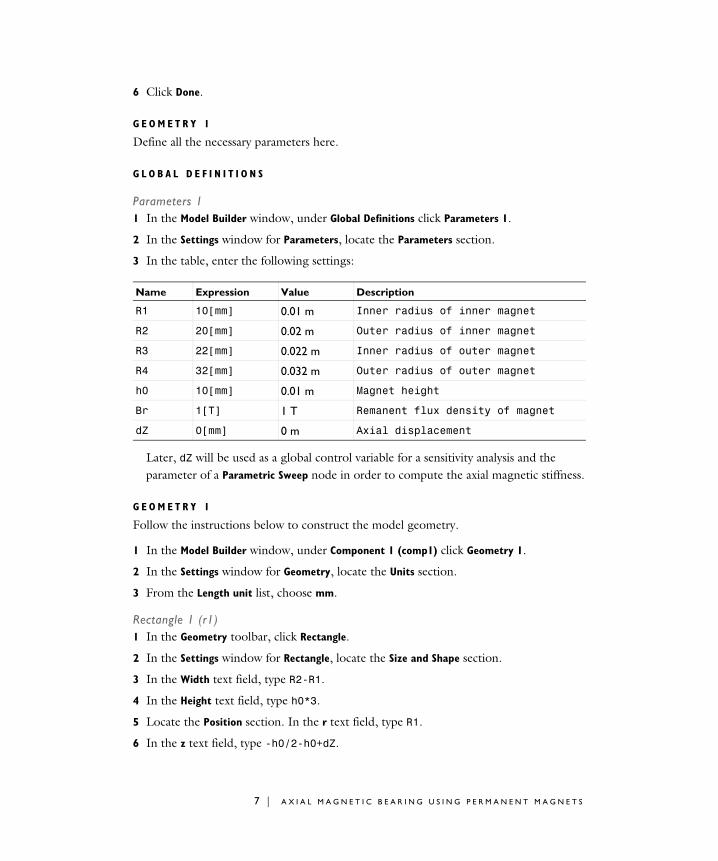
3 On the object r2, select Points 1, 4, 5, and 8 only.
4 In the Settings window for Fillet, locate the Radius section.
5 In the Radius text field, type 2.
6 Click Build All Objects.
7 Click the Zoom Extents button in the Graphics toolbar.
The model geometry should look like the one shown in the figure above.
9 | A X I A L M A G N E T I C B E A R I N G U S I N G P E R M A N E N T M A G N E T S

Enclose the inner air domain by an Infinite Element Domain to model the surrounding space.
Infinite Element Domain 1 (ie1)1 In the Definitions toolbar, click Infinite Element Domain.
2 Select Domains 1, 3, and 10–12 only.
3 In the Settings window for Infinite Element Domain, locate the Geometry section.
4 From the Type list, choose Cylindrical.
M A T E R I A L S
Use air as the material for all domains and override it in permanent magnets with a material that will be created based on a modification of an existing entry from library.
1 In the Home toolbar, click Windows and choose Add Material from Library.
A D D M A T E R I A L
1 Go to the Add Material window.
2 In the tree, select Built-in>Air.
3 Click Add to Component in the window toolbar.
4 In the tree, select AC/DC>Hard Magnetic Materials>
Sintered NdFeB Grades (Chinese Standard)>N50 (Sintered NdFeB).
5 Click Add to Component 1 (comp1).
10 | A X I A L M A G N E T I C B E A R I N G U S I N G P E R M A N E N T M A G N E T S
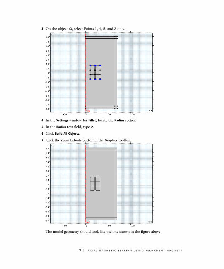
6 In the Home toolbar, click Add Material to close the Add Material window.
M A T E R I A L S
N50 (Sintered NdFeB) (mat2)1 Select Domains 4–9 only.
2 In the Settings window for Material, locate the Material Contents section.
3 In the table, enter the following settings:
4 In the Label text field, type Generic magnet.
Now set up the physics for the magnetic field: use the default Magnetic Flux Conservation node with default settings for the air domains and add separate nodes for the magnets (one per magnetization direction).
M A G N E T I C F I E L D S , N O C U R R E N T S ( M F N C )
Magnetic Flux Conservation 21 In the Model Builder window, under Component 1 (comp1) right-click Magnetic Fields,
No Currents (mfnc) and choose Magnetic Flux Conservation.
2 Select Domains 6 and 9 only.
3 In the Settings window for Magnetic Flux Conservation, locate the Constitutive Relation B-
H section.
4 From the Magnetization model list, choose Remanent flux density.
5 Specify the e vector as
Property Variable Value Unit Property group
Recoil permeability murec_iso ; murecii = murec_iso, murecij = 0
1 1 Remanent flux density
Remanent flux density norm normBr Br T Remanent flux density
0 r
0 phi
-1 z
11 | A X I A L M A G N E T I C B E A R I N G U S I N G P E R M A N E N T M A G N E T S

Magnetic Flux Conservation 31 In the Physics toolbar, click Domains and choose Magnetic Flux Conservation.
2 Select Domains 4 and 7 only.
3 In the Settings window for Magnetic Flux Conservation, locate the Constitutive Relation B-
H section.
4 From the Magnetization model list, choose Remanent flux density.
5 Specify the e vector as
Magnetic Flux Conservation 41 In the Physics toolbar, click Domains and choose Magnetic Flux Conservation.
2 Select Domain 5 only.
3 In the Settings window for Magnetic Flux Conservation, locate the Constitutive Relation B-
H section.
4 From the Magnetization model list, choose Remanent flux density.
Magnetic Flux Conservation 51 In the Physics toolbar, click Domains and choose Magnetic Flux Conservation.
2 Select Domain 8 only.
3 In the Settings window for Magnetic Flux Conservation, locate the Constitutive Relation B-
H section.
4 From the Magnetization model list, choose Remanent flux density.
5 Specify the e vector as
Force Calculation 1Add a Force Calculation feature to compute the total magnetic force on the inner magnets.
1 In the Physics toolbar, click Domains and choose Force Calculation.
0 r
0 phi
1 z
-1 r
0 phi
0 z
12 | A X I A L M A G N E T I C B E A R I N G U S I N G P E R M A N E N T M A G N E T S

2 Select Domains 4–6 only.
Keeping the default force name, 0, the axial force component can be accessed as mfnc.Forcez_0, where mfnc is the identifier for the Magnetic Fields, No Currents interfaces.
Specify a reference level for the magnetic scalar potential by constraining its value in one point.
Zero Magnetic Scalar Potential 11 In the Physics toolbar, click Points and choose Zero Magnetic Scalar Potential.
2 Select Point 30 only.
Next, add the Moving Mesh and Sensitivity interfaces to use for calculating the axial magnetic stiffness coefficient as defined by Equation 1 of the Model Definition section.
A D D P H Y S I C S
1 In the Physics toolbar, click Add Physics to open the Add Physics window.
2 Go to the Add Physics window.
3 In the tree, select Mathematics>Optimization and Sensitivity>Sensitivity (sens).
4 Click Add to Component 1 in the window toolbar.
5 In the Physics toolbar, click Add Physics to close the Add Physics window.
S E N S I T I V I T Y ( S E N S )
With the Sensitivity interface you can compute the right-hand side of Equation 1 as the derivative of the global objective defined as the axial force component mfnc.Forcez_0 with respect to the global control variable defined as the axial displacement dZ.
Global Control Variables 11 Right-click Component 1 (comp1)>Sensitivity (sens) and choose Global Control Variables.
2 In the Settings window for Global Control Variables, locate the Control Variables section.
3 In the Control variables table, enter the following settings:
Global Objective 11 In the Physics toolbar, click Global and choose Global Objective.
2 In the Settings window for Global Objective, locate the Global Objective section.
3 In the q text field, type mfnc.Forcez_0.
Variable Initial value
dZ 0
13 | A X I A L M A G N E T I C B E A R I N G U S I N G P E R M A N E N T M A G N E T S

D E F I N I T I O N S
Deforming Domain 11 In the Definitions toolbar, click Moving Mesh and choose Deforming Domain.
2 Select Domain 2 only.
Prescribed Deformation 1In the Definitions toolbar, click Moving Mesh and choose Prescribed Deformation.
Deforming Domain 11 In the Model Builder window, click Deforming Domain 1.
2 In the Settings window for Deforming Domain, locate the Smoothing section.
3 From the Mesh smoothing type list, choose Laplace.
Prescribed Deformation 11 Click the Select All button in the Graphics toolbar.
2 In the Model Builder window, click Prescribed Deformation 1.
3 In the Settings window for Prescribed Deformation, locate the Geometric Entity Selection section.
4 Click Clear Selection.
5 Click the Select Box button in the Graphics toolbar.
6 Select Domains 4–6 only.
7 Locate the Prescribed Deformation section. Specify the dx vector as
Prescribed Mesh Displacement 11 In the Definitions toolbar, click Moving Mesh and choose Prescribed Mesh Displacement.
2 Select Boundaries 3, 4, 6, 18, 19, 21, 23–27, 30, and 42–45 only.
M E S H 1
1 In the Model Builder window, under Component 1 (comp1) click Mesh 1.
2 In the Settings window for Mesh, click Build All.
0 R
dZ Z
14 | A X I A L M A G N E T I C B E A R I N G U S I N G P E R M A N E N T M A G N E T S
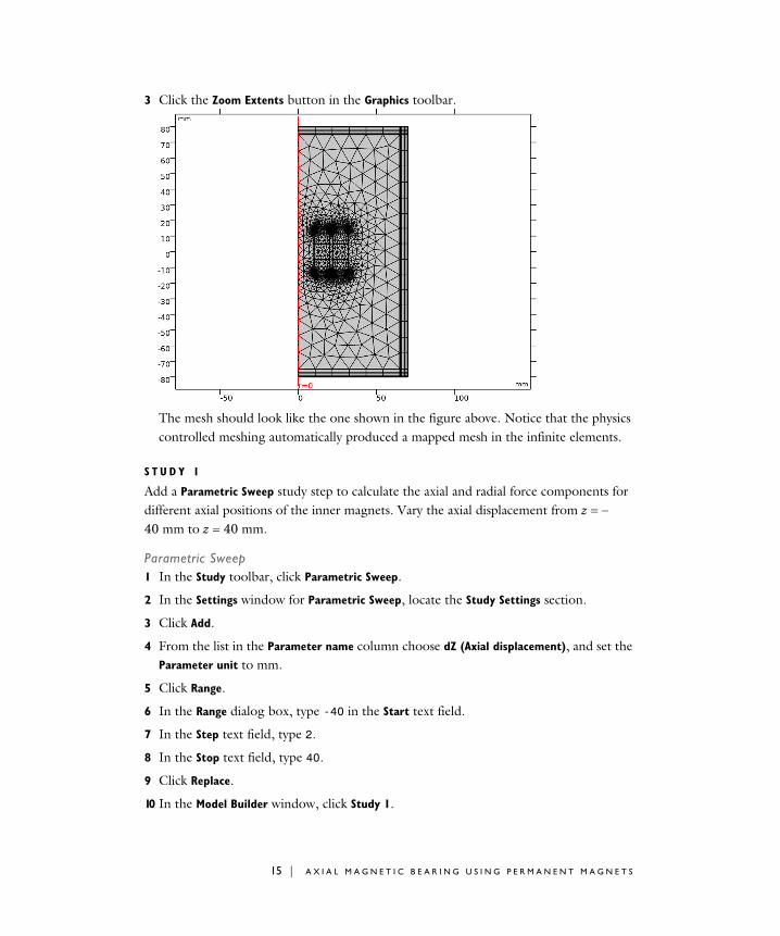
3 Click the Zoom Extents button in the Graphics toolbar.
The mesh should look like the one shown in the figure above. Notice that the physics controlled meshing automatically produced a mapped mesh in the infinite elements.
S T U D Y 1
Add a Parametric Sweep study step to calculate the axial and radial force components for different axial positions of the inner magnets. Vary the axial displacement from z 40 mm to z 40 mm.
Parametric Sweep1 In the Study toolbar, click Parametric Sweep.
2 In the Settings window for Parametric Sweep, locate the Study Settings section.
3 Click Add.
4 From the list in the Parameter name column choose dZ (Axial displacement), and set the Parameter unit to mm.
5 Click Range.
6 In the Range dialog box, type -40 in the Start text field.
7 In the Step text field, type 2.
8 In the Stop text field, type 40.
9 Click Replace.
10 In the Model Builder window, click Study 1.
15 | A X I A L M A G N E T I C B E A R I N G U S I N G P E R M A N E N T M A G N E T S

11 In the Settings window for Study, locate the Study Settings section.
12 Clear the Generate default plots check box.
Solution 1 (sol1)1 In the Study toolbar, click Show Default Solver.
2 In the Model Builder window, expand the Solution 1 (sol1) node.
3 Right-click Stationary Solver 1 and choose Sensitivity.
4 In the Study toolbar, click Compute.
R E S U L T S
In the Model Builder window, expand the Results node.
Study 1/Parametric Solutions 1 (sol2)Create data sets for result visualization in specific domains.
Study 1/Parametric Solutions 1 (3) (sol2)1 In the Model Builder window, expand the Results>Datasets node.
2 Right-click Results>Datasets>Study 1/Parametric Solutions 1 (sol2) and choose Duplicate.
3 In the Settings window for Solution, locate the Solution section.
4 From the Solution list, choose dZ=8 (sol27).
Selection1 In the Results toolbar, click Attributes and choose Selection.
2 In the Settings window for Selection, locate the Geometric Entity Selection section.
3 From the Geometric entity level list, choose Domain.
4 Select Domains 4–9 only.
Revolution 2D 11 In the Results toolbar, click More Datasets and choose Revolution 2D.
2 In the Settings window for Revolution 2D, locate the Data section.
3 From the Dataset list, choose Study 1/dZ=8 (sol27).
4 Click to expand the Revolution Layers section. In the Start angle text field, type -100.
5 In the Revolution angle text field, type 280.
Use the following instructions to get the plots shown in Figure 2 to Figure 5.
2D Plot Group 1In the Results toolbar, click 2D Plot Group.
16 | A X I A L M A G N E T I C B E A R I N G U S I N G P E R M A N E N T M A G N E T S
Surface 11 Right-click 2D Plot Group 1 and choose Surface.
2 In the Settings window for Surface, click Replace Expression in the upper-right corner of the Expression section. From the menu, choose Component 1>Magnetic Fields,
No Currents>Magnetic>mfnc.normB - Magnetic flux density norm - T.
3 In the 2D Plot Group 1 toolbar, click Plot.
Streamline 11 In the Model Builder window, right-click 2D Plot Group 1 and choose Streamline.
2 In the Settings window for Streamline, locate the Streamline Positioning section.
3 From the Positioning list, choose Uniform density.
4 In the Separating distance text field, type 0.02.
5 Locate the Coloring and Style section. Find the Point style subsection. From the Color list, choose Gray.
6 In the 2D Plot Group 1 toolbar, click Plot.
7 Click the Zoom Extents button in the Graphics toolbar.
Compare this plot with Figure 2.
1D Plot Group 2In the Home toolbar, click Add Plot Group and choose 1D Plot Group.
Global 11 Right-click 1D Plot Group 2 and choose Global.
2 In the Settings window for Global, locate the Data section.
3 From the Dataset list, choose Study 1/Parametric Solutions 1 (sol2).
4 Locate the y-Axis Data section. Click Clear Table.
5 Click Replace Expression in the upper-right corner of the y-axis data section. From the menu, choose Component 1>Sensitivity>sens.gobj1 - Objective value - N.
6 In the 1D Plot Group 2 toolbar, click Plot.
Compare the plot just created with that shown in Figure 3.
1D Plot Group 3In the Home toolbar, click Add Plot Group and choose 1D Plot Group.
Global 11 Right-click 1D Plot Group 3 and choose Global.
2 In the Settings window for Global, locate the Data section.
17 | A X I A L M A G N E T I C B E A R I N G U S I N G P E R M A N E N T M A G N E T S

3 From the Dataset list, choose Study 1/Parametric Solutions 1 (sol2).
4 Locate the y-Axis Data section. Click Clear Table.
5 In the table, enter the following settings:
6 In the 1D Plot Group 3 toolbar, click Plot.
Compare this plot with Figure 4.
3D Plot Group 4Finally, reproduce Figure 5 using the following steps.
In the Home toolbar, click Add Plot Group and choose 3D Plot Group.
Volume 11 Right-click 3D Plot Group 4 and choose Volume.
2 In the Settings window for Volume, click Replace Expression in the upper-right corner of the Expression section. From the menu, choose mfnc.normB - Magnetic flux density norm - T.
3 In the 3D Plot Group 4 toolbar, click Plot.
Expression Unit Description
fsens(dZ) N/m Sensitivity of Fz w.r.t. dZ
18 | A X I A L M A G N E T I C B E A R I N G U S I N G P E R M A N E N T M A G N E T S