This is an electronic reprint of the original article.This reprint may differ from the original in pagination and typographic detail.

Powered by TCPDF (www.tcpdf.org)

This material is protected by copyright and other intellectual property rights, and duplication or sale of all or part of any of the repository collections is not permitted, except that material may be duplicated by you for your research use or educational purposes in electronic or print form. You must obtain permission for any other use. Electronic or print copies may not be offered, whether for sale or otherwise to anyone who is not an authorised user.

Awan, Hafiz; Song, Zhanfeng; Saarakkala, Seppo E.; Hinkkanen, MarkoOptimal torque control of saturated synchronous motors: plug-and-play method

Published in:IEEE Transactions on Industry Applications

DOI:10.1109/TIA.2018.2862410

Published: 02/08/2018

Document VersionPeer reviewed version

Please cite the original version:Awan, H., Song, Z., Saarakkala, S. E., & Hinkkanen, M. (2018). Optimal torque control of saturated synchronousmotors: plug-and-play method. IEEE Transactions on Industry Applications, 54(6), 6110-6120.https://doi.org/10.1109/TIA.2018.2862410

1

Optimal Torque Control of SaturatedSynchronous Motors: Plug-and-Play Method

Hafiz Asad Ali Awan, Zhanfeng Song, Member, IEEE, Seppo E. Saarakkala, andMarko Hinkkanen, Senior Member, IEEE

Abstract—This paper deals with the optimal state referencecalculation for synchronous motors having a magnetically salientrotor. A look-up table computation method for the maxi-mum torque-per-ampere (MTPA) locus, maximum torque-per-volt (MTPV) limit, and field-weakening operation is presented.The proposed method can be used during the start-up of a drive,after the magnetic model identification. It is computationallyefficient enough to be implemented directly in the embeddedprocessor of the drive. When combined with an identificationmethod for the magnetic model, the proposed method enablesthe plug-and-play start-up of an unknown motor. Furthermore,a conventional reference calculation scheme is improved byremoving the need for one two-dimensional look-up table. A6.7-kW synchronous reluctance motor (SyRM) drive is used forexperimental validation.

Index Terms—Optimal control, synchronous motor drives,torque control.

I. INTRODUCTION

SYNCHRONOUS motors with a magnetically salientrotor—such as a synchronous reluctance motor (SyRM),

a permanent-magnet (PM)-SyRM, and an interior PM syn-chronous motor—are well suited for hybrid or electric ve-hicles, heavy-duty working machines, and industrial applica-tions [1]–[5]. These machines often exhibit highly nonlinearsaturation characteristics, which should be properly takeninto account in the control system in order to reach highperformance. At the same time, a quick start-up procedureis desirable, especially in industrial applications.

Fig. 1 exemplifies a control system of a typical current-controlled drive. The motor is driven at the maximum torque-per-ampere (MTPA) locus, at the current limit, at the maxi-mum torque-per-volt (MTPV) limit, or in the field-weakeningregion (which is the region bounded by the above-mentionedlocus and limits), depending on the torque reference Tref , theoperating speed ωm, and the DC-bus voltage udc. This paperfocuses on the calculation of the optimal state references forthe fastest control loop, i.e., the current references id,ref andiq,ref in the example control system shown in the figure.

In most existing control methods, the MTPA locus andthe MTPV limit are either computed off-line based on the

Conference version “Optimal torque control of synchronous motor drives:Plug-and-play method” was presented at the 2017 IEEE Energy ConversionCongress and Exposition (ECCE), Cincinnati, OH, Oct. 1–5. This work wassupported in part by ABB Oy Drives and in part by the Academy of Finland.

H. A. A. Awan, S. E. Saarakkala, and M. Hinkkanen are with theSchool of Electrical Engineering, Aalto University, Espoo, Finland (e-mail:hafiz.awan@aalto.fi; seppo.saarakkala@aalto.fi; marko.hinkkanen@aalto.fi).

Z. Song is with the School of Electrical and Information Engineering,Tianjin University, Tianjin, China (e-mail: zfsong@tju.edu.cn).

id,ref

ϑm

iabc

M

Currentcontrol

udc

Tref Referencecalculation

d

dt

ωm

Magneticmodel

identification

Look-uptable

computation

Plug-and-play start-up

iq,ref

Fig. 1. Control system of a typical current-controlled drive (the lower part),augmented with a plug-and-play start-up method (the upper part). The start-up method consists of two stages, magnetic model identification and look-up table computation, which can be run in the embedded processor of thedrive. Look-up tables are then used in the reference calculation. The currentcontroller operates in rotor coordinates; the electrical angle of the rotor isdenoted by ϑm. The control system may include a speed controller, whichprovides the torque reference.

known magnetic saturation characteristics or measured witha suitable test bench. The resulting look-up tables are thenimplemented in the real-time control system. The off-linecomputation as well as test-bench measurements are typicallytime-consuming processes. Instead of using an MTPA look-uptable, the MTPA locus could be tracked using signal injection[6], which, however, causes additional noise and losses. Insome applications, an approximate MTPV limit could besearched for in an iterative manner by means of repeatedacceleration tests [7].

Field-weakening methods can be broadly divided into feed-back methods [8]–[12] and feedforward methods [13]–[20].The feedback field-weakening methods apply the differencebetween the reference voltage and the maximum availablevoltage. These methods use the maximum voltage in the field-weakening operation, but they do not necessary guarantee min-imum losses. The voltage control loop has to be properly tunedand should have much lower bandwidth than the innermostcurrent controller [12]. Furthermore, the MTPA locus and theMTPV limit are needed in the feedback methods as well.

The feedforward field-weakening methods provide the opti-mal references without delays. Due to the feedforward natureof these methods, the dynamics of the inner control loopremain intact and the noise content in the state referencesis minor. However, modeling inaccuracies may reduce the

2

available torque or increase the losses. Some feedforward field-weakening methods are based on analytical solutions of theintersection of a voltage ellipse and a torque hyperbola [13]–[15]. A disadvantage of these methods is that they do not takethe magnetic saturation into account (and the saturation effectscannot be properly taken into account afterwards, since thesaturation deforms the shape of the voltage ellipses and torquehyperbolas). Other feedforward methods are based on off-linecomputed look-up tables [16]–[20]. The magnetic saturationcan be included properly in these methods, but the off-linedata processing is difficult and time-consuming, even thoughsome open-source post-processing algorithms are available[21]. Feedforward methods based on the finite-element method(FEM) rely on the knowledge of the motor geometry [16],[18]. Furthermore, the feedforward methods can be augmentedwith an additional voltage controller in order to be able todynamically adjust the voltage margin [19], [20].

We consider a plug-and-play start-up method for optimalreference calculation, originally presented in the conferenceversion [22] of this paper. As illustrated in Fig. 1, the magneticmodel of the motor is first identified and the control look-uptables are then computed. These two tasks are executed off-line during the start-up, preferably in the embedded processorof the drive. After the start-up has been completed, thecontrol look-up tables are ready to be used in the real-timecontrol. After defining the motor model in Section II, the maincontributions are presented as follows:• A conventional reference calculation scheme [17]–[20],

applicable to feedforward field-weakening, is improvedby removing the need for one two-dimensional look-uptable in Section III.

• A look-up table computation method is proposed in Sec-tion IV. When combined with an identification methodfor the magnetic model, the proposed method enablesthe plug-and-play start-up of an unknown motor. Variousidentification methods for the magnetic model of SyRMs,PM-SyRMs, and interior PM synchronous motors arealready available [23]–[25].

• The effects of model uncertainties on the current lociand the achievable torque are analyzed in Section V.The proposed method is also evaluated by means ofsimulations and experiments.

The current-controlled drive is used as an example, but thelook-up table computation method (or its part) could also beused in connection with other control methods. If, e.g., thedirect-flux vector control were used, only the MTPA locusand the MTPV limit would be needed [7].

II. MOTOR MODEL

A. Fundamental Equations

The motor model in rotor coordinates is considered, asshown in Fig. 2. The stator voltage equations are

dψd

dt= ud −Rid + ωmψq (1a)

dψq

dt= uq −Riq − ωmψd (1b)

Ld

id R

uddψd

dt

ωmψq

if

Lq

iq R

uqdψq

dt

ωmψd

Fig. 2. Equivalent circuit of a PM synchronous motor. The saturableinductances Ld and Lq are described by (7). The constant current sourceif models the MMF due to the PMs.

where id and iq are the current components, ψd and ψq

are the flux linkage components, ud and uq are the voltagecomponents, ωm is the electrical angular speed of the rotor,and R is the stator resistance. The current components

id = id(ψd, ψq) iq = iq(ψd, ψq) (2)

are generally nonlinear functions of the flux components. Theyare the inverse of the flux maps, often represented by two-dimensional look-up tables. Here, the modeling approach (2)is chosen, because it is more favorable towards representationin the algebraic form. Since the nonlinear inductor shouldnot generate or dissipate electrical energy, the reciprocitycondition [26]

∂id∂ψq

=∂iq∂ψd

(3)

should hold. Typically, the core losses are either omitted ormodeled separately using a core-loss resistor in the model.

The produced torque is

T =3p

2(ψdiq − ψqid) (4)

where p is the number of pole pairs. If the functions (2) and thestator resistance are known, the machine is fully characterizedboth in the steady and transient states. For example, the MTPAlocus can be resolved from (2) and (4). In the following, thecurrent magnitude will be denoted by

i =√i2d + i2q (5)

The similar notation is used for the voltage and flux linkagemagnitudes as well.

B. Algebraic Magnetic Model

The constant current source if in the equivalent circuit inFig. 2 represents the magnetomotive force (MMF) of the PMs[1]. The structure of the equivalent circuit is based on theassumption that the MMFs of the d-axis current and of the PMsare in series. Under this assumption, an algebraic magneticmodel [24], originally developed for SyRMs, can be extendedto the PM synchronous machines as

id =

(ad0 + add|ψd|α +

adqδ + 2

|ψd|γ |ψq|δ+2

)ψd − if (6a)

iq =

(aq0 + aqq|ψq|β +

adqγ + 2

|ψd|γ+2|ψq|δ)ψq (6b)

where ad0, add, aq0, aqq, and adq are non-negative coefficientsand α, β, γ, and δ are non-negative exponents. The coefficient

3

(a)

(b)

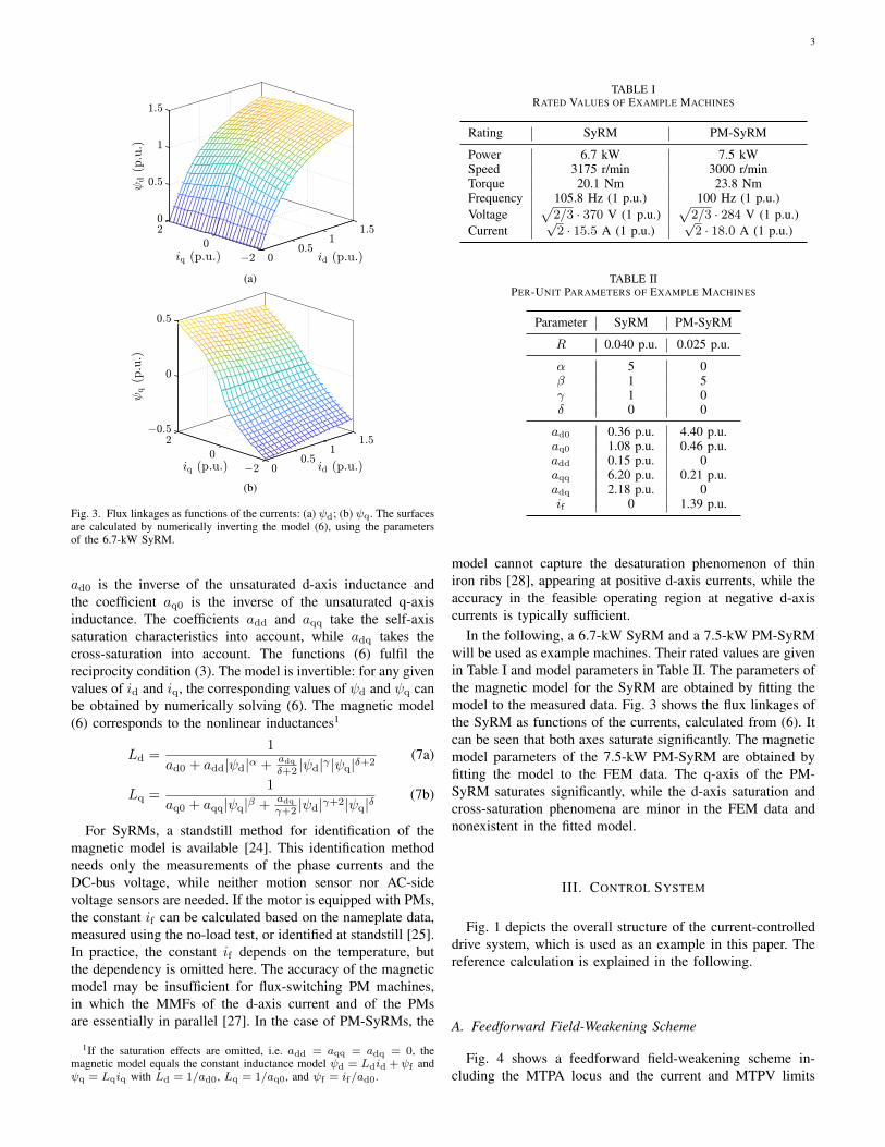
Fig. 3. Flux linkages as functions of the currents: (a) ψd; (b) ψq. The surfacesare calculated by numerically inverting the model (6), using the parametersof the 6.7-kW SyRM.

ad0 is the inverse of the unsaturated d-axis inductance andthe coefficient aq0 is the inverse of the unsaturated q-axisinductance. The coefficients add and aqq take the self-axissaturation characteristics into account, while adq takes thecross-saturation into account. The functions (6) fulfil thereciprocity condition (3). The model is invertible: for any givenvalues of id and iq, the corresponding values of ψd and ψq canbe obtained by numerically solving (6). The magnetic model(6) corresponds to the nonlinear inductances1

Ld =1

ad0 + add|ψd|α +adq

δ+2 |ψd|γ |ψq|δ+2(7a)

Lq =1

aq0 + aqq|ψq|β +adq

γ+2 |ψd|γ+2|ψq|δ(7b)

For SyRMs, a standstill method for identification of themagnetic model is available [24]. This identification methodneeds only the measurements of the phase currents and theDC-bus voltage, while neither motion sensor nor AC-sidevoltage sensors are needed. If the motor is equipped with PMs,the constant if can be calculated based on the nameplate data,measured using the no-load test, or identified at standstill [25].In practice, the constant if depends on the temperature, butthe dependency is omitted here. The accuracy of the magneticmodel may be insufficient for flux-switching PM machines,in which the MMFs of the d-axis current and of the PMsare essentially in parallel [27]. In the case of PM-SyRMs, the

1If the saturation effects are omitted, i.e. add = aqq = adq = 0, themagnetic model equals the constant inductance model ψd = Ldid + ψf andψq = Lqiq with Ld = 1/ad0, Lq = 1/aq0, and ψf = if/ad0.

TABLE IRATED VALUES OF EXAMPLE MACHINES

Rating SyRM PM-SyRM

Power 6.7 kW 7.5 kWSpeed 3175 r/min 3000 r/minTorque 20.1 Nm 23.8 NmFrequency 105.8 Hz (1 p.u.) 100 Hz (1 p.u.)Voltage

√2/3 · 370 V (1 p.u.)

√2/3 · 284 V (1 p.u.)

Current√2 · 15.5 A (1 p.u.)

√2 · 18.0 A (1 p.u.)

TABLE IIPER-UNIT PARAMETERS OF EXAMPLE MACHINES

Parameter SyRM PM-SyRM

R 0.040 p.u. 0.025 p.u.

α 5 0β 1 5γ 1 0δ 0 0

ad0 0.36 p.u. 4.40 p.u.aq0 1.08 p.u. 0.46 p.u.add 0.15 p.u. 0aqq 6.20 p.u. 0.21 p.u.adq 2.18 p.u. 0if 0 1.39 p.u.

model cannot capture the desaturation phenomenon of thiniron ribs [28], appearing at positive d-axis currents, while theaccuracy in the feasible operating region at negative d-axiscurrents is typically sufficient.

In the following, a 6.7-kW SyRM and a 7.5-kW PM-SyRMwill be used as example machines. Their rated values are givenin Table I and model parameters in Table II. The parameters ofthe magnetic model for the SyRM are obtained by fitting themodel to the measured data. Fig. 3 shows the flux linkages ofthe SyRM as functions of the currents, calculated from (6). Itcan be seen that both axes saturate significantly. The magneticmodel parameters of the 7.5-kW PM-SyRM are obtained byfitting the model to the FEM data. The q-axis of the PM-SyRM saturates significantly, while the d-axis saturation andcross-saturation phenomena are minor in the FEM data andnonexistent in the fitted model.

III. CONTROL SYSTEM

Fig. 1 depicts the overall structure of the current-controlleddrive system, which is used as an example in this paper. Thereference calculation is explained in the following.

A. Feedforward Field-Weakening Scheme

Fig. 4 shows a feedforward field-weakening scheme in-cluding the MTPA locus and the current and MTPV limits

4

Tref

ωm

min(·)

ψmtpa

ψref

Tmax

udc

min(·)T ref

sign(·)

| · |

| · |

umaxku/√3

ψmax

Fig. 4. Feedforward field-weakening scheme including the MTPA locus andthe current and MTPV limits. The optimal flux magnitude is ψref and the lim-ited torque reference is T ref . The torque limit is Tmax = min(Tmtpv, Tlim),where Tlim corresponds to the maximum current and Tmtpv corresponds tothe MTPV limit. The factor ku defines the voltage margin.

T ref

id,ref

ψref

iq,ref

sign(·)

| · |

(a)

T ref

ψd,ref

ψq,refsign(·)

√ψ2ref − ψ2

d,ref

| · |

ψref

id,ref

iq,refEq.(6)

(b)

Fig. 5. Current references: (a) conventional method [17]–[20]; (b) proposedmethod with only one two-dimensional look-up table.

[7], [17]–[20]. From (1), the stator voltage magnitude can beexpressed as

u =√u2d + u2q

=

√(ωmψq −Rid −

dψd

dt

)2

+

(ωmψd +Riq +

dψq

dt

)2

(8)

If R = 0 and the steady state are assumed, this expression forthe voltage magnitude reduces to u = |ωm|ψ, which is used toconvert the maximum available voltage umax to the maximumavailable flux magnitude ψmax in the scheme shown in Fig. 4.

The maximum voltage umax = kuudc/√

3 is calculatedfrom the measured DC-link voltage udc. Hence, any suddenvariations in udc are directly translated into the references.The factor ku defines the voltage margin. As can be realizedfrom (8), some voltage reserve is necessary for the resistivevoltage drops and for changing the flux linkages in transientconditions. If ku = 1 is chosen, the overmodulation region

may be entered even in the steady state (due to the resistivevoltage drops), which causes the sixth harmonics in the statorvoltage. To avoid entering the overmodulation region in thesteady state, the factor ku < 1 should be chosen. Alternatively,the resistive voltage drops could be compensated for by meansof the measured current and the resistance estimate, cf. e.g.[7]. However, applying this feedback action in the referencecalculation may introduce increased noise content and ringingphenomena. It is also worth noticing that the factor ku couldbe dynamically adjusted by means of an additional voltagecontroller [19], [20]. For simplicity, a constant value for ku isused in this paper.

As seen in Fig. 4, the optimal MTPA flux magnitudeψmtpa is read from a look-up table, whose input is the torquereference. The MTPA flux is limited based on the maximumflux ψmax, yielding the optimal flux magnitude ψref underthe voltage constraint. The torque reference Tref is limited bythe torque Tmax corresponding to the combined MTPV andcurrent limits, yielding the limited torque reference T ref . Anadvantage of the scheme shown in Fig. 4 is that the optimalreference values are obtained without any delays. The schemecan also be used in connection with other control schemes,such as the direct-flux vector control.

B. Current References

If the current-controlled drive is used, the optimal fluxreference and the limited torque reference have to be mappedto the corresponding current references. Fig. 5(a) shows theconventional current reference calculation method [17]–[20],based on the two two-dimensional look-up tables. Interpolationis used to get the values of id,ref and iq,ref from the look-uptables.

Fig. 5(b) shows the proposed current reference calculationmethod. A single two-dimensional look-up table is used todetermine ψd,ref . Then, the value of the q-axis flux ψq,ref

is obtained by means of the Pythagorean theorem. The flux-linkage references are mapped to the current references using(6). Since only one two-dimensional look-up table is needed,the memory requirements of the control system are lessthan in the conventional method. An interpolation procedure,applicable to the conventional method as well, is given in theAppendix.

IV. LOOK-UP TABLE COMPUTATION

Fig. 6 shows an overall diagram of the look-up tablecomputation method, which is divided into four stages. Inthe following equations, Ld ≤ Lq is assumed. Further, thed-axis of the coordinate system is fixed to the direction ofthe PMs (or along the minimum inductance axis), withoutloss of generality. After the look-up table computation, thed- and q-axes of the SyRM are flipped to the standard SyRMrepresentation, i.e., the d-axis along the maximum inductanceaxis. In this section, the notation and terminology is simplifiedsuch that we do not particularly refer to the reference quantities(e.g., ψ is used instead of ψref ). It should be clear from thecontext how the resulting look-up tables are used in the real-time control system.

5

MTPV

Output list: {Tmtpv(m)}

M

compute (14)for m = 1 :M

Input list: {ψ(m)}

MTPA

Output lists: {ψmtpa(l)}, {Tmtpa(l)}

L, imax

compute (10)–(12)for l = 1 : L

Input list: {i(l)}

ψmtp

a(L

)

Current limit

Output list: {Tlim(m)}

for m = 1 :M

Input list: {ψ(m)}

compute (15)

{ψd,m

tpv(m

)}Reference look-up table

Output table: {ψd,ref(m,n)}

for m = 1 :M

Input lists: {ψ(m)}, {Tref(n)}

for n = 1 :M

compute (17)

{Tmtp

v(m

)}

Fig. 6. Look-up table computation procedure. The parameters of the magneticmodel (6) are also needed in each stage.

The look-up table computation method is not limited to thesaturation model (6). Different magnetic models or even look-up tables could be used instead, if they are physically feasibleand invertible in the relevant operation range. Furthermore,the reference calculation method corresponding to Figs. 4 and5(b) is used as an example, but the proposed look-up tablecomputation method can be easily modified for other referencecalculation structures as well.

A. MTPA

For creating a look-up table, a list of L equally-spacedcurrent magnitudes is defined

{i(l)} = (l − 1)∆i, l = 1, 2, . . . L (9)

where ∆i = imax/(L− 1) and imax is the maximum current.For each current magnitude i, the maximum torque Tmtpa andthe corresponding argument id,mtpa are obtained by solvingthe optimization problem

Tmtpa = maxid∈[−i,0]

T (id) (10a)

(a)

(b)

Fig. 7. Look-up tables for the MTPA locus, MTPV limit, and current limit:(a) 6.7-kW SyRM; (b) 7.5-kW PM-SyRM. The id = 0 line does not need tobe computed, but it is shown just for illustration purposes. L = 20 is used inthese plots. The rated torque is denoted by TN.

where the torque is expressed as a function of id

T (id) =3p

2[ψd(id, iq) · iq(id)− ψq(id, iq) · id] (10b)

iq(id) =√i2 − i2d (10c)

and the search interval is −i ≤ id ≤ 0. The flux componentsψd and ψq corresponding to id and iq are calculated bynumerically inverting the algebraic magnetic model (6), i.e.,

(ψd, ψq) = solveψd,ψq

{id(ψd, ψq) = idiq(ψd, ψq) = iq

}(11)

After solving (10), the optimal q-component iq,mtpa is ob-tained from (10c).

The optimal flux magnitude is

ψmtpa =√ψ2d,mtpa + ψ2

q,mtpa (12)

where ψd,mtpa and ψq,mtpa corresponding to id,mtpa andiq,mtpa are obtained using (11). The Brent algorithm [29] isused for solving (10) without using derivatives. The Powelldogleg algorithm [30] is used for inverting the magnetic modelin (11).

As shown in Fig. 6, the procedure (10)–(12) is repeated ina for loop for each element i(l) of the list (9). Then, a look-up table for the control system, cf. Fig. 4, is created fromthe resulting lists {ψmtpa(l)} and {Tmtpa(l)}. As illustratedin Fig. 6, the inputs to the MTPA computation stage are thenumber of points L to be computed, the maximum currentimax, and the parameters of the magnetic model (6). MTPAloci are generally comparatively smooth and, typically, L

6

around 10–20 suffices. The maximum current imax is selectedbased on the motor and converter ratings.

Fig. 7(a) shows the computed MTPA look-up table for the6.7-kW SyRM and Fig. 7(b) for the 7.5-kW PM-SyRM. In thecontrol algorithm, the optimal flux reference magnitude ψref

is obtained based on this look-up table, as shown in Fig. 4.

B. MTPV

For creating the look-up table, a list of M equally-spacedstator flux magnitudes is defined

{ψ(m)} = (m− 1)∆ψ, m = 1, 2, . . .M (13)

where ∆ψ = ψmtpa(L)/(M − 1), i.e., the maximum fluxmagnitude ψmtpa(L) is the result from the last step of theMTPA computation. For each flux magnitude ψ, the maximumtorque Tmtpv is obtained by solving

Tmtpv = maxψd∈[−ψ,0]

T (ψd) (14a)

where the torque is expressed as

T (ψd) =3p

2[ψd · iq(ψd, ψq)− ψq(ψd) · id(ψd, ψq)] (14b)

ψq(ψd) =√ψ2 − ψ2

d (14c)

The magnetic model (6) is directly used in (14b), i.e., nomagnetic model inversion is needed in this stage. The Brentalgorithm is used for solving the optimization problem (14).

As shown in Fig. 6, the problem (14) is solved for eachelement ψ(m) of the list (13). Then, the look-up table forthe control system is created using the resulting output list{Tmtpv(m)}. Fig. 7 shows the computed MTPV look-up tablesfor the two machines.

C. Maximum Current Limit

The already defined input list (13) of the flux magnitudes isconsidered. For each flux magnitude ψ(m), the d-componentψd,lim of the flux corresponding to the maximum current imax

is solved

ψd,lim = solveψd∈[ψd,mtpv,ψd,max]

{i2(ψd) = i2max

}(15a)

where the square of the current magnitude is expressed as

i2(ψd) = i2d(ψd, ψq) + i2q(ψd, ψq) (15b)

ψq(ψd) =√ψ2 − ψ2

d (15c)

The lower bound ψd,mtpv in (15) is the d-component of theMTPV flux at each ψ and the upper bound ψd,max is the d-component of the MTPA flux at the maximum current. After(15) has been solved, the corresponding torque Tlim is obtainedfrom (14b). The Brent algorithm is used to solve this boundednonlinear problem.

As shown in Fig. 6, the problem (15) is solved for eachelement ψ(m). The lower bounds {ψd,mtpv(m)} needed in(15) have already been computed during the MTPV stage.The upper bound ψd,max = ψd,mtpa(L) is the d-component ofthe MTPA flux at the maximum current imax and it has alsobeen computed. From the resulting output list {Tlim(m)}, a

(a)

(b)

Fig. 8. Flux component ψd as a function of ψ and T : (a) 6.7-kW SyRM;(b) 7.5-kW PM-SyRM. The feasible operating region is limited by the MTPAlocus, the MTPV limit, and the current limit, which are also plotted. Look-uptables are not computed beyond the id = 0 line. They are applied in thecontrol system according to Fig. 5(b). M = 50 is used in these plots.

look-up table for the control system is created. Fig. 7 showsthe computed current limits of two times the rated current forthe SyRM and the PM-SyRM. The MTPV and current limitscan be easily merged into one limit

Tmax = min (Tmtpv, Tlim) (16)

D. Two-Dimensional Reference Look-Up Table

For given flux magnitude ψ and torque reference Tref , thed-component ψd,ref is solved

ψd,ref = solveψd∈[ψd,mtpv,ψ]

{Tref = T (ψd)} (17)

where the torque T (ψd) is given by (14b). The lower boundψd,mtpv is the d-component of the MTPV flux at ψ. The Brentalgorithm is used to solve (17).

For creating the look-up table, (17) can be solved in twonested for loops. As an input to one loop, the list (13) ofthe flux magnitudes {ψ(m)} is used. In the other loop, thealready calculated MTPV torque values {Tmtpv(m)} can beused as an input, i.e. {Tref(n)} = {Tmtpv(m)}. This selectionnot only defines the maximum torque which can be generated(under the MTPV limit) but also explicitly gives the lowerbound ψd,mtpv for each ψd,ref . If the maximum current isfixed, {Tref(n)} = {Tmax(m)} can be used instead. The look-up table for the control system is created from the resultingtable {ψd,ref(m,n)}. Fig. 8 shows the two-dimensional look-up tables for the two machines. The id = 0 line shown in Fig.

7

(a) (b)

Fig. 9. MTPA locus, MTPV limit, and current limit for the 6.7-kW SyRM:(a) id–iq plane; (b) ψd–ψq plane. The dashed lines show the loci, whenthe magnetic saturation is not taken into account (inductances correspond tothe rated operating point). The black dashed line corresponds to the constantcurrent circle.

(a) (b)

Fig. 10. MTPA locus, MTPV limit, and current limit for the 7.5-kWPM-SyRM: (a) id–iq plane; (b) ψd–ψq plane. The dashed lines show theloci, when the magnetic saturation is not taken into account (inductancescorrespond to the rated operating point). The black dashed line correspondsto the constant current circle.

8(b) does not need to be computed, but it is shown just forillustration purposes.

E. Generalization for Machines With Ld > Lq

Some special PM machines can have Ld > Lq [31]. Thepresented algorithm can be easily modified to include thesemachines as well. Only a few modifications in the ranges areneeded: id ∈ [−i, i] in (10); ψd ∈ [−ψ,ψ] in (14); and ψd ∈[−ψd,mtpv, ψ] in (15). In this general case, the computationtime of the algorithm will increase.

V. RESULTS

The computed look-up tables and the reference calculationscheme corresponding to Figs. 4 and 5(b) are evaluated bymeans of analysis, simulations, and experiments. The param-eters used for the look-up table computation are: L = 10;M = 150; and imax = 2 p.u. The parameters of the magneticmodel (6) given in Table II are also needed. The computationtime for the look-up tables is less than 35 s in an Androidmobile phone. We expect that the computation time is slightlylonger in a typical digital-signal processor applied in frequencyconverters.

(a)

(b)

Fig. 11. Maximum torque vs. speed characteristics for the 6.7-kW SyRM:(a) effect of omitting the magnetic saturation in the reference calculation; (b)different current limits. In (a), the blue line shows the case where the magneticsaturation is taken into account, the red line shows the case where the cross-saturation is omitted (adq = 0), and the green line shows the case where therated constant inductances are used in the reference calculation. The currentlimit was set to 2 p.u. In (b), three different current limits are shown. Theonset of the field weakening are marked with circles and the MTPV limit bycrosses.

A. Analysis

The effect of the magnetic saturation on the optimal ref-erences is analyzed. Fig. 9 shows the current references inthe id–iq plane and the flux references in the ψd–ψq plane forthe 6.7-kW SyRM. The solid lines correspond to the computedoptimal values, while the magnetic saturation is omitted in thecase of the dashed lines. The effect of the saturation is clearlyvisible: using constant inductances would result in non-optimaloperating points. Fig. 10 shows the corresponding loci for the7.5-kW PM-SyRM. The saturation affects mainly the MTPAlocus in this case.

Fig. 11(a) shows the effect of the magnetic saturationon the maximum torque production for the 6.7-kW SyRM.It can be seen that the torque production capability dropssignificantly, if the magnetic saturation is omitted in thereference calculation and the inductances in the rated operatingpoint are used instead. Furthermore, the cross-saturation alsohas a significant effect on the torque production. This resultindicates that the cross-saturation effect should be included inthe magnetic model in the case of SyRMs. Fig. 11(b) showsthe maximum torque versus speed characteristics for differentcurrent limits. If needed, the reference calculation scheme in

8

(a) (b)

Fig. 12. Simulation results showing acceleration from zero to 2 p.u. with two different voltage margins: (a) ku = 0.8; (b) ku = 1. The first subplot showsthe reference speed ωm,ref and the actual speed ωm. The second subplot shows the reference torque Tref and the estimated torque T . The third subplotshows the reference and measured current components. The last subplot shows the magnitude uref of the reference voltage, the maximum available voltageudc/

√3 in the linear modulation range, and the maximum voltage umax = kuudc/

√3 in the steady state.

Fig. 4 can be modified easily to use multiple current limits oreven a dynamic current limit, as needed in some industrialapplications. Three to four one-dimensional look-up tablescould be used for different current limits and then the resultsbetween these limits could be interpolated as required.

The effect of the core losses on the torque productioncapability is analyzed for the 6.7-kW SyRM. For this analysis,the constant core-loss resistance of 18 p.u., correspondingto [32], has been included in the motor model. Since thecore losses are omitted in the proposed reference calculationmethod, the achieved maximum torque is 6% less than thereal maximum torque at the speed of 1.25 p.u. The loss of theachievable maximum torque increases with the speed. Effectsof the core losses on the efficiency have been analyzed in [19],[32].

B. Simulations

Simulations and experiments were performed on the 6.7-kW SyRM drive. The magnetic saturation in the motor modeland the controller is modeled using the magnetic model in(6). The load torque is modeled as the viscous friction. Thetotal moment of inertia is 0.03 kgm2. The space-vector pulse-width modulator and the discrete-time current controller [33]are used. The sampling and switching frequency are 5 kHz.The speed controller bandwidth is 10 Hz.

Fig. 12(a) shows the acceleration test when the voltagemargin is defined by ku = 0.8. The motor is acceleratedfrom zero to the speed of 2 p.u. It can be seen that themeasured currents follow their references well. The magnitudeuref of the voltage reference, the limit udc/

√3 of the linear-

modulation range, and the desired maximum steady-statevoltage umax = kuudc/

√3 are also shown. It can be seen

that the overmodulation range is not entered in this case.Fig. 12(b) shows the same test with ku = 1. It can be

seen that the overmodulation range is mostly used during theacceleration. Furthermore, the current iq deviates from its ref-erence during the acceleration. This behavior is expected sinceonly part of the overmodulation voltage reserve is available forchanging the currents in transient operation, cf. (8). However,due to the higher value of the stator flux linkage with ku = 1,the acceleration time is shorter than with ku = 0.8.

A suitable choice for the voltage margin factor ku dependson the application. In these examples, the speed referencewas changed stepwise. However, the speed reference signalis typically ramped, which decreases the need for the voltagemargin. As discussed in Section III, the feedforward field-weakening method could be augmented with a voltage con-troller providing a dynamic voltage margin, which allowscombining the maximum utilization of the DC-bus voltage inthe steady state with proper tracking of the current referencesin transients.

9

(a) (b)

Fig. 13. Experimental results showing acceleration from zero to 2 p.u. with two different voltage margins: (a) ku = 0.8; (b) ku = 1.

(a) (b)

Fig. 14. Experimental results showing torque reference steps at two different speeds: (a) ωm = 0.6 p.u.; (b) ωm = 1.2 p.u.

C. Experiments

The reference calculation scheme corresponding to Figs.4 and 5(b) was experimentally evaluated together with thecomputed look-up tables. The controller was implemented ona dSPACE DS1006 processor board. The rotor speed ωm ismeasured using an incremental encoder. The stator currentsand the DC-link voltage are measured.

Fig. 13 shows the experimental results corresponding tothe simulation results in Fig. 12. It can be seen that theexperimental results and the simulation results match verywell. There is a slight overshoot in the speed response at theend of the acceleration due to imperfect tuning of the speed

controller, further causing the torque reference to change itssign momentarily.

Fig. 14 shows the results for the constant speed tests at twodifferent speeds. The load drive of the test bench regulatesthe speed and the drive under test is driven in the torque-control mode. Fig. 14(a) shows the results when the speed isregulated at 0.6 p.u. The torque reference is stepped from zeroto 150% of the rated torque with increments of 25%. Fig. 14(b)shows the results when the speed is regulated at 1.2 p.u. andthe torque reference is stepped from zero to the rated torquewith increments of 25%. The current dynamics in this kindof constant speed tests are governed solely by the closed-loop

10

current control dynamics, as can be realized from Figs. 1, 4,and 5(b). The reference calculation scheme maps the torquereference to the optimal current references in a feedforwardmanner without any dynamics.

VI. CONCLUSIONS

A look-up table computation algorithm for the MTPA locus,MTPV limit, and feedforward field-weakening operation ispresented. The algorithm can be used during the drive start-up,after the magnetic model identification. It is computationallyefficient enough to be implemented directly in the embeddedprocessor of the drive. Alternatively, the look-up tables couldbe computed remotely using the algorithm and then uploadedto the drive, if the drive is connected to a cloud server or to amobile phone. A conventional real-time reference calculationscheme was also improved by removing the need for onetwo-dimensional look-up table. The importance of includingthe magnetic saturation in the look-up table computation washighlighted. Using constant inductances would result in non-optimal operating points, as the saturation deforms the voltageellipses and torque hyperbolas. The proposed method properlytakes the magnetic saturation into account. The computedlook-up tables and the reference calculation scheme wereevaluated using experiments on a 6.7-kW SyRM drive.

APPENDIXINTERPOLATION

Generally, four points are needed for the interpolation intwo dimensions. However, no data is available for the two-dimensional look-up table beyond the MTPV limit. Hence,when operating in the vicinity of the MTPV limit, only threepoints are available for the interpolation algorithm. Therefore,there are two different modes in the interpolation algorithm,as described in the following.

Suppose that the value of a function f is available at fourpoints (x1, y1), (x1, y2), (x2, y1), and (x2, y2) shown in Fig.15. The value of the function at (x, y) can be approximatedusing bilinear interpolation

f(x, y) =

[x2 − xx− x1

]T [f(x1, y1) f(x1, y2)f(x2, y1) f(x2, y2)

] [y2 − yy − y1

](x2 − x1)(y2 − y1)

(18)

If the value at one point, e.g. at (x2, y1), is not available,the values at the remaining three points can be used forapproximating the value at (x, y) by means of a plane equation

f(x, y) = ax+ by + c (19)

where abc

=

x1 y1 1x1 y2 1x2 y2 1

−1 f(x1, y1)f(x1, y2)f(x2, y2)

(20)

For interpolating ψd at the point (ψ, T ), the four pointssurrounding (ψ, T ) are read from the look-up table and(18) is then applied. If only three points are available dueto the vicinity of the MTPV limit, (19) is applied insteadof (18). The value of the q-axis flux component ψq could

x1 x x2

y1

y

(x1, y2)y2

(x1, y1) (x2, y1)

(x2, y2)

(x, y)

Fig. 15. Four points (x1, y1), (x1, y2), (x2, y1), and (x2, y2) used forinterpolating the value at (x, y).

be calculated from the final interpolated result ψd using thePythagorean theorem, but it might create chattering in thecalculated reference. Instead, the q-axis flux component is firstcalculated using the Pythagorean theorem at all the three orfour points used in the interpolation algorithm for ψd. To getthe interpolated ψq, either (18) or (19) is used, depending onthe number of the points.

ACKNOWLEDGMENT

The authors would like to thank Prof. G. Pellegrino forproviding the flux map data of the 7.5-kW PM-SyRM.

REFERENCES

[1] T. M. Jahns, G. B. Kliman, and T. W. Neumann, “Interior permanent-magnet synchronous motors for adjustable-speed drives,” IEEE Trans.Ind. Appl., vol. IA-22, no. 4, pp. 738–747, July 1986.

[2] W. L. Soong and T. J. E. Miller, “Field-weakening performance ofbrushless synchronous AC motor drives,” IEE Proc. Electr. Power Appl.,vol. 141, no. 6, pp. 331–340, Nov. 1994.

[3] Z. Q. Zhu and D. Howe, “Electrical machines and drives for electric,hybrid, and fuel cell vehicles,” Proc. IEEE, vol. 95, no. 4, pp. 746–765,Apr. 2007.

[4] G. Pellegrino, A. Vagati, B. Boazzo, and P. Guglielmi, “Comparisonof induction and PM synchronous motor drives for EV applicationincluding design examples,” IEEE Trans. Ind. Appl., vol. 48, no. 6, pp.2322–2332, Nov. 2012.

[5] N. Bianchi, S. Bolognani, E. Carraro, M. Castiello, and E. Fornasiero,“Electric vehicle traction based on synchronous reluctance motors,”IEEE Trans. Ind. Appl., vol. 52, no. 6, pp. 4762–4769, Nov. 2016.

[6] S. Kim, Y.-D. Yoon, S.-K. Sul, and K. Ide, “Maximum torque per ampere(MTPA) control of an IPM machine based on signal injection consider-ing inductance saturation,” IEEE Trans. Power Electron., vol. 28, no. 1,pp. 488–497, Jan. 2013.

[7] G. Pellegrino, E. Armando, and P. Guglielmi, “Direct-flux vector controlof IPM motor drives in the maximum torque per voltage speed range,”IEEE Trans. Ind. Electron., vol. 59, no. 10, pp. 3780–3788, Oct. 2012.

[8] J.-M. Kim and S.-K. Sul, “Speed control of interior permanent magnetsynchronous motor drive for the flux weakening operation,” IEEE Trans.Ind. Appl., vol. 33, no. 1, pp. 43–48, Jan. 1997.

[9] Y.-C. Kwon, S. Kim, and S.-K. Sul, “Voltage feedback current controlscheme for improved transient performance of permanent magnet syn-chronous machine drives,” IEEE Trans. Ind. Electron., vol. 59, no. 9,pp. 3373–3382, Sept. 2012.

[10] P.-Y. Lin, W.-T. Lee, S.-W. Chen, J.-C. H., and Y.-S. Lai, “Infinite speeddrives control with MTPA and MTPV for interior permanent magnetsynchronous motor,” in Proc. IEEE IECON, Dallas, TX, Oct. 2014, pp.668–674.

[11] K. D. Hoang and H. K. A. Aorith, “Online control of IPMSM drivesfor traction applications considering machine parameter and inverternonlinearities,” IEEE Trans. Transport. Electrific., vol. 1, no. 4, pp. 312–325, Dec. 2015.

11

[12] N. Bedetti, S. Calligaro, and R. Petrella, “Analytical design of flux-weakening voltage regulation loop in IPMSM drives,” in Proc. ECCE,Montreal, Canada, Sept. 2015, pp. 6145–6152.

[13] S. Morimoto, Y. Takeda, T. Hirasa, and K. Taniguchi, “Expansion ofoperating limits for permanent magnet motor by current vector controlconsidering inverter capacity,” IEEE Trans. Ind. Appl., vol. 26, no. 5,pp. 866–871, Sept./Oct. 1990.

[14] S.-Y. Jung, J. Hong, and K. Nam, “Current minimizing torque controlof the IPMSM using Ferrari’s method,” IEEE Trans. Power Electron.,vol. 28, no. 12, pp. 5603–5617, Dec. 2013.

[15] I. Jeong, B.-G. Gu, J. Kim, K. Nam, and Y. Kim, “Inductance estimationof electrically excited synchronous motor via polynomial approximationsby least square method,” IEEE Trans. Ind. Appl., vol. 51, no. 2, pp.1526–1537, Mar. 2013.

[16] M. H. Mohammadi and D. A. Lowther, “A computational study ofefficiency map calculation for synchronous ac motor drives includingcross-coupling and saturation effects,” IEEE Trans. Magn., vol. 53, no. 6,pp. 1–4, June 2017.

[17] M. Meyer and J. Bocker, “Optimum control for interior permanentmagnet synchronous motors (IPMSM) in constant torque and fluxweakening range,” in Proc. EPE-PEMC, Portoroz, Slovenia, Aug./Sept.2006, pp. 282–286.

[18] H. W. de Kock, A. Rix, and M. J. Kamper, “Optimal torque control ofsynchronous machines based on finite-element analysis,” IEEE Trans.Ind. Electron., vol. 57, no. 1, pp. 413–419, Jan. 2010.

[19] W. Peters, O. Wallscheid, and J. Bocker, “Optimum efficiency control ofinterior permanent magnet synchronous motors in drive trains of electricand hybrid vehicles,” in Proc. EPE ECCE-Europe, Geneva, Switzerland,Sept. 2015, pp. 1–10.

[20] T. Huber, W. Peters, and J. Bocker, “Voltage controller for flux weak-ening operation of interior permanent magnet synchronous motor inautomotive traction applications,” in Proc. IEMDC, Coeur d’Alene, ID,May 2015, pp. 1078–1083.

[21] Synchronous reluctance (machines) - evolution. [Online]. Available:https://sourceforge.net/projects/syr-e/

[22] H. A. A. Awan, Z. Song, S. E. Saarakkala, and M. Hinkkanen, “Optimaltorque control of synchronous motor drives: Plug-and-play method,” inProc. IEEE ECCE, Cincinnati, OH, Oct. 2017, pp. 334–341.

[23] N. Bedetti, S. Calligaro, and R. Petrella, “Stand-still self-identificationof flux characteristics for synchronous reluctance machines using novelsaturation approximating function and multiple linear regression,” IEEETrans. Ind. Appl., vol. 52, no. 4, pp. 3083–3092, July/Aug. 2016.

[24] M. Hinkkanen, P. Pescetto, E. Molsa, S. E. Saarakkala, G. Pellegrino,and R. Bojoi, “Sensorless self-commissioning of synchronous reluctancemotors at standstill without rotor locking,” IEEE Trans. Ind. Appl.,vol. 53, no. 3, pp. 2120–2129, May/June 2017.

[25] P. Pescetto and G. Pellegrino, “Sensorless magnetic model and PM fluxidentification of synchronous drives at standstill,” in Proc. IEEE SLED,Catania, Italy, Sept. 2017, pp. 79–84.

[26] A. Vagati, M. Pastorelli, F. Scapino, and G. Franceschini, “Impact ofcross saturation in synchronous reluctance motors of the transverse-laminated type,” IEEE Trans. Ind. Appl., vol. 36, no. 4, pp. 1039–1046,July/Aug. 2000.

[27] Z. Q. Zhu, Y. Pang, D. Howe, S. Iwasaki, R. Deodhar, and A. Pride,“Analysis of electromagnetic performance of flux-switching permanent-magnet machines by nonlinear adaptive lumped parameter magneticcircuit model,” IEEE Trans. Magn., vol. 41, no. 11, pp. 4277–4288,Nov. 2005.

[28] E. Armando, P. Guglielmi, G. Pellegrino, M. Pastorelli, and A. Vagati,“Accurate modeling and performance analysis of IPM-PMASR motors,”IEEE Trans. Ind. Appl., vol. 45, no. 1, pp. 123–130, Jan. 2009.

[29] R. P. Brent, Algorithms for minimization without derivatives. Mineola,NY: Dover Publ., 2013.

[30] M. J. D. Powell, “An efficient method for finding the minimum ofa function of several variables without calculating derivatives,” TheComput. J., vol. 7, no. 2, pp. 155–162, Jan. 1964.

[31] N. Bianchi, S. Bolognani, and B. J. Chalmers, “Salient-rotor PMsynchronous motors for an extended flux-weakening operation range,”IEEE Trans. Ind. Appl., vol. 36, no. 4, pp. 1118–1125, July./Aug. 2000.

[32] Z. Qu, T. Tuovinen, and M. Hinkkanen, “Minimizing losses of asynchronous reluctance motor drive taking into account core losses andmagnetic saturation,” in Proc. EPE, Lappeenranta, Finland, Aug. 2014.

[33] M. Hinkkanen, H. A. A. Awan, Z. Qu, T. Tuovinen, and F. Briz,“Current control for synchronous motor drives: direct discrete-time pole-placement design,” IEEE Trans. Ind. Appl., vol. 52, no. 2, pp. 1530–1541, Mar./Apr. 2016.

Hafiz Asad Ali Awan received the B.Sc. degree inelectrical engineering from the University of Engi-neering and Technology, Lahore, Pakistan, in 2012,and the M.Sc.(Tech.) degree in electrical engineeringfrom Aalto University, Espoo, Finland, in 2015.

He is currently working toward the D.Sc.(Tech.)degree at Aalto University. His main research inter-est include control of electric drives.

Zhanfeng Song (M’13) was born in Hebei, China,in 1982. He received the B.S., M.S., and Ph.D.degrees from Tianjin University, Tianjin, China, in2004, 2006, and 2009, respectively, all in electricalengineering.

He is currently an Associate Professor with theSchool of Electrical and Information Engineering,Tianjin University. His research interests includepredictive control of electrical machines and powerconverters.

Seppo E. Saarakkala received the M.Sc.(Eng.) de-gree in electrical engineering from the LappeenrantaUniversity of Technology, Lappeenranta, Finland,in 2008, and the D.Sc.(Tech.) degree in electricalengineering from Aalto University, Espoo, Finland,in 2014.

He has been with the School of Electrical En-gineering, Aalto University, since 2010, where heis currently a Post-Doctoral Research Scientist. Hismain research interests include control systems andelectric drives.

Marko Hinkkanen (M’06–SM’13) received theM.Sc.(Eng.) and D.Sc.(Tech.) degrees in electricalengineering from the Helsinki University of Tech-nology, Espoo, Finland, in 2000 and 2004, respec-tively.

He is an Associate Professor with the School ofElectrical Engineering, Aalto University, Espoo. Hisresearch interests include control systems, electricdrives, and power converters.

Dr. Hinkkanen was the corecipient of the 2016International Conference on Electrical Machines

(ICEM) Brian J. Chalmers Best Paper Award and the 2016 IEEE IndustryApplications Society Industrial Drives Committee Best Paper Award. He isan Editorial Board Member of IET Electric Power Applications.