SU(3)F Analysis for Beauty Baryon Decays

Avital Dery,∗ Mitrajyoti Ghosh,† Yuval Grossman,‡ and Stefan Schacht§

Department of Physics, LEPP, Cornell University, Ithaca, NY 14853, USA

AbstractWe perform a general SU(3)F analysis of b → ccs(d) decays of members of the beauty

baryon antitriplet to a member of the light baryon octet and a singlet. Under several

reasonable assumptions we found∣∣A(Ξ0

b → ΛS)/A(Ξ0b → Ξ0S)

∣∣ ≈ 1/√

6 |V ∗cbVcd/(V ∗cbVcs)| and∣∣A(Λb → Σ0S)/A(Λb → ΛS)∣∣ ∼ 0.02. These two relations have been recently probed by LHCb

for the case of S = J/ψ. The former agrees with the measurement, while for the latter our predic-

tion lies close to the upper bound set by LHCb.

∗ avital.dery@cornell.edu† mg2338@cornell.edu‡ yg73@cornell.edu§ ss3843@cornell.edu

1

arX

iv:2

001.

0539

7v2

[he

p-ph

] 2

Apr

202

0

I. INTRODUCTION

A tremendous amount of b-baryons is produced at the LHC [1]. This allows for angular

analyses of Λb decays at LHCb [2] and ATLAS [3] and has led to evidence of CP violation

in Λb decays [4]. It is now feasible to scrutinize rare or suppressed b-baryon decays: Recent

results include the first observation of Λb → Λγ [5] and the analysis of the isospin suppressed

Λb → Σ0J/ψ decay and the Cabibbo-suppressed decay Ξ0b → ΛJ/ψ [6].

These increasingly precise measurements of baryon decays motivate us to perform an

SU(3)F analysis of b → ccq (with q = s, d) decays of the heavy b-baryon 3 to the light

baryon 8 and an SU(3)F singlet, 3b → 8b ⊗ 1. From the perspective of SU(3)F it makes no

difference if the singlet, which we denote as S, is a J/ψ or any final state particle that does

not carry any SU(3)F flavor, for example, a photon or a lepton pair.

We start our analysis using two separate assumptions: (1) We work in the SU(3)F limit

and (2) we treat the Λ and Σ0 as isospin eigenstates. We emphasize that these assumptions

are not connected to each other. We later relax these assumptions and take into account

corrections to the SU(3)F limit as well as deviations of the mass eigenstates of Λ and Σ0

from their isospin eigenstates.

At leading order the decays 3b → 8b ⊗ 1 are mediated by tree-level b → ccq transitions.

These correspond to a 3 operator. In full generality however, we have to take into account

additional contributions from loops that generate effective b→ ttq and b→ uuq transitions.

The contribution from b→ ttq can be neglected as it is a penguin and therefore suppressed

and it gives only another 3 under SU(3)F . In contrast, the up quarks in b→ uuq can induce

intermediate on-shell states leading to nontrivial effects from rescattering. Specifically, the

b → uuq transition has a more complicated isospin and SU(3)F structure and induces the

higher SU(3)F representations 6 and 15. Therefore, as higher SU(3)F representations stem

from rescattering, in the literature it is often assumed that these are suppressed.

Our strategy is to start with a very general model-independent viewpoint and then in-

troduce additional assumptions step by step. While we mainly concentrate in this paper on

the case where S = J/ψ, the general nature of our results make it possible to apply them

also to radiative and semileptonic decays.

CKM-leading SU(3)F limit Clebsch-Gordan coefficients for 3b → 8b ⊗ 1 in b→ s transi-

tions have been presented in Refs. [7–9]. In Refs. [8, 10–12] hadronic models based on QCD

2

factorization have been utilized, and in Refs. [9, 13] a covariant confined quark model has

been applied. An SU(3)F analysis of b-baryon antitriplet decays to the light baryon octet

and the η1 singlet can be found in Ref. [14].

Further applications of SU(3)F to b baryon decays can be found in Refs. [15–20]. Works

on b baryon decays beyond their SU(3)F treatment are given in Refs. [21–25]. Applications

of SU(3)F methods on non-b baryon decays can be found in Refs. [26–37]. Further literature

on baryon decays is given in Refs. [38–40]. Discussions of baryonic form factors can be found

in Refs. [41–50].

We present our SU(3)F analysis including isospin and SU(3)F breaking in Sec. II. After

that we estimate in Sec. III the effect of Σ0–Λ mixing in Λb decays, which is in general scale-

and process-dependent, i.e. non-universal. We compare with recent experimental results in

Sec. IV and conclude in Sec. V.

II. SU(3)F ANALYSIS

A. General SU(3)F Decomposition

The b → ccq (with q = s, d) decays of Λb, Ξ−b and Ξ0b , which form the heavy baryon 3,

into a singlet S (e.g. S = J/ψ, γ, l+l−, . . . ) and a member of the light baryon 8, share a

common set of reduced SU(3)F matrix elements after the application of the Wigner-Eckart

theorem. These decays are specifically:

• b→ scc transitions:

Λb → ΛS , Λb → Σ0S , Ξ0b → Ξ0S , Ξ−b → Ξ−S . (1)

• b→ dcc transitions:

Ξ0b → ΛS , Ξ0

b → Σ0S , Λb → nS , Ξ−b → Σ−S . (2)

Note that there are two additional allowed decays Λb → Ξ0J/ψ and Ξ0b → nJ/ψ which

are however highly suppressed by two insertions of weak effective operators, so we do not

consider them in our study here. The SU(3)F quantum numbers and masses are given in

Table I. In this section we discuss the SU(3)F limit, SU(3)F -breaking effects are treated in

Sec. II E.

3

We can write the SU(3)F structure of the relevant b→ s and b→ d Hamiltonians as [51]

Hb→s = λcs(cb)(sc) + λus(ub)(su) + λts(tb)(st)

= λcs (3)c0,0,− 23

+ λus

((3)u0,0,− 2

3+ (6)

u1,0,− 2

3+√

6 (15)u1,0,− 23

+√

3 (15)u0,0,− 23

), (3)

Hb→d = λcd(cb)(dc) + λud(ub)(du) + λtd(tb)(dt)

= λcd (3)c12,− 1

2, 13

+ λud

((3)u1

2,− 1

2, 13−(6)u

12,− 1

2, 13

+√

8 (15)u32,− 1

2, 13

+ (15)u12,− 1

2, 13

). (4)

See also Refs. [52] and [53] for the application of these Hamiltonians to B → J/ψK and

B → DD, respectively. The notation for the subindices are such that (N)I,I3,Y refers to

the irreducible representation N of SU(3)F using the quantum numbers of strong isospin I,

I3 and strong hypercharge Y . In the standard basis of the Gell-Mann matrices I3 and Y

correspond to the eigenvalues of λ3 and λ8, respectively. We further use the notation

λcs ≡ V ∗cbVcs ∼ λ2 , λus ≡ V ∗ubVus ∼ λ4 , λts ≡ V ∗tbVts ∼ λ2 , (5)

λcd ≡ V ∗cbVcd ∼ λ3 , λud ≡ V ∗ubVud ∼ λ3 , λtd ≡ V ∗tbVtd ∼ λ3 , (6)

for the CKM matrix element combinations, where we indicate the hierarchies using the

Wolfenstein parameter λ.

Note that in Eqs. (3) and (4) it is understood that SU(3)F operators in front of different

CKM matrix elements have to be differentiated as they stem from different underlying op-

erators. For instance, even if the two triplets generate linearly dependent Clebsch-Gordan

coefficients, the respective matrix elements themselves are independent. They can, for ex-

ample, have a relative strong phase.

We write the reduced SU(3)F limit matrix elements as Akq , where k is the respective

SU(3)F representation in the Hamiltonian and q denotes the operator it stems from. The

initial state is always a∣∣3⟩ and the final state is always a |8〉, so that we are left with four

reduced matrix elements in the SU(3)F limit:

A3c , A3

u , A6u , A15

u . (7)

The SU(3)F limit decomposition is given in Table II. The CKM-leading part of the b → s

transitions agrees with Refs. [7–9]. The Clebsch-Gordan coefficients are obtained using

Refs. [54–56]. The normalization of the amplitudes is such that

B(B1 → B2S) = |A(B1 → B2S)|2 × P(B1, B2, S) , (8)

4

with the two-body decay phase space factors

P(B1, B2, S) ≡ τB1

16πm3B1

√(m2

B1− (mB2 −mS)2)(m2

B1− (mB2 +mS)2) . (9)

Note that in cases where the SU(3)F singlet S is a multibody state, e.g. S = l+l−, we

imply the appropriate phase space integration in Eq. (8). Note further, that we still work

in the SU(3)F limit of the decay amplitudes. Eq. (9) only accounts for the trivial SU(3)F

breaking from phase space effects. Additional SU(3)F breaking contributions are discussed

in Sec. II E. Therein, we estimate SU(3)F breaking effects to be of order 20%. Note that the

amplitudes in Eq. (8) have a mass dimension, but we always care about ratios, so we can

think about them as dimensionless quantities. Note that phase space effects are of order 3%

and thus they are well within the errors and could or could not be taken into account. For

a model-dependent way to estimate these effects one can, for example, employ form factor

results in Refs. [9, 57].

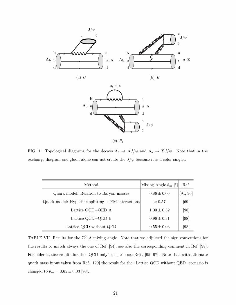
The reduced SU(3)F matrix elements can in principle be matched on a color suppressed

tree diagram C, an exchange diagram E and penguin diagrams Pq with quark q running in

the loop. As examples we show the topological diagrams for Λb → ΛJ/ψ and Λb → Σ0J/ψ

in Fig. 1. In the following, however, we only perform the group theory treatment.

The combined matrix of Clebsch-Gordan coefficients of b → s and b → d decays in

Table II has matrix rank four, i.e., there are four sum rules, which read

−√

3

2A(Λb → ΛS) +

1√2A(Λb → Σ0S) +A(Ξ0

b → Ξ0S) = 0 , (SU(3)F sum rule) (10)√3

2A(Ξ0

b → ΛS)− 1√2A(Ξ0

b → Σ0S) +A(Λb → nS) = 0 , (SU(3)F sum rule) (11)

−√

2A(Λb → Σ0S)λudλus

+√

6A(Ξ0b → ΛS) +A(Λb → nS) = 0 , (SU(3)F sum rule) (12)√

3

2A(Λb → ΛS)

λudλus− 3√

2A(Λb → Σ0S)

λudλus

−A(Ξ−b → Ξ−S)λudλus

+√

6A(Ξ0b → ΛS) +A(Ξ−b → Σ−S) = 0 , (SU(3)F sum rule) (13)

all of which are SU(3)F sum rules, and there is no isospin sum rule. Note that there are two

sum rules which mix b → s and b → d decays and two which do not. These sum rules are

valid in the SU(3)F limit irrespective of the power counting of the CKM matrix elements,

assumptions on the reduced matrix elements, or the particular SU(3)F singlet S, i.e. they

are completely generic.

5

B. Assumptions on CKM Hierarchy and Rescattering

We now make some assumptions, which are not completely generic, i.e. their validity can

for example depend on the particular considered SU(3)F singlet S, e.g. if S = J/ψ or S = γ.

We first neglect the CKM-suppressed amplitude in b→ s decays, that is we set λus/λcs →

0. In the isospin and SU(3)F limit for b → s decays we have then only one contributing

reduced matrix element:

A(Λb → Σ0S) = 0 , (isospin sum rule) (14)

A(Ξ0b → Ξ0S) = A(Ξ−b → Ξ−S) , (isospin sum rule) (15)

A(Ξ0b → Ξ0S) =

√3

2A(Λb → ΛS) . (SU(3)F sum rule) (16)

We now move to make another assumption and that is to also neglect the λud terms for

the b → d transitions. Despite the formal power counting Eq. (6), that is |λud| ' |λcd|,

numerically we actually have [58]

∣∣∣∣λudλcd

∣∣∣∣ ≈ 0.38 . (17)

Moreover, it is plausible that A6u and A15

u are suppressed because they result from light

quarks stemming from b→ uus(d) which induce intermediate on-shell states that rescatter

into cc, see also Refs. [59–63]. Under the assumption that these terms are more or equally

suppressed as SU(3)F -breaking effects we have many more relations. All seven non-zero

decays we considered in Table II are then simply related by the Clebsch-Gordan coefficients

in the first column. In addition to the sum rules Eqs. (14)–(16), we have then

√2A(Ξ0

b → Σ0S) = A(Ξ−b → Σ−S) , (isospin sum rule) (18)

A(Ξ0b → Ξ0S) = −

√6A(Ξ0

b → ΛS)λcsλcd

, (SU(3)F sum rule) (19)

−√

6A(Ξ0b → ΛS) =

√2A(Ξ0

b → Σ0S) , (SU(3)F sum rule) (20)√

2A(Ξ0b → Σ0S) = A(Λb → nS) , (SU(3)F sum rule) (21)

A(Λb → nS) = A(Ξ−b → Σ−S) . (SU(3)F sum rule) (22)

6

C. Isospin and U-Spin Decompositions

For comprehensiveness, we give also the isospin and U -spin decompositions of the Hamil-

tonians, which read

Hb→s = λcs(0, 0)cI + λus ((0, 0)uI + (1, 0)uI ) (23)

= λcs

(1

2,−1

2

)cU

+ λus

(1

2,−1

2

)uU

, (24)

and

Hb→d = λcd

(1

2,−1

2

)cI

+ λud

((3

2,−1

2

)uI

+

(1

2,−1

2

)uI

)(25)

= λcd

(1

2,1

2

)cU

+ λud

(1

2,1

2

)uU

, (26)

where we use the notation

(i, j)qI ≡ O∆I=i∆I3=j , (i, j)qU ≡ O

∆U=i∆U3=j , (27)

where q denotes the quark content of the operator the representation stems from and we

absorbed Clebsch-Gordan coefficients into operators.

Using the isospin and U -spin states in Table I, we obtain the isospin decompositions

in Tables III and IV and the U -spin decomposition in Table V. We note that the SU(3)F

decomposition includes more information than the isospin and U -spin tables each on their

own. An example is the ratio∣∣∣∣ A(Ξ0b → ΛS)

A(Ξ0b → Ξ0S)

∣∣∣∣ =1√2

∣∣∣∣∣ 〈0| 12

∣∣12

⟩⟨12

∣∣ 0 ∣∣12

⟩∣∣∣∣∣∣∣∣∣λcdλcs

∣∣∣∣ . (28)

where the appearing reduced matrix elements are not related, e.g. the final states belong

to different isospin representations. That means we really need SU(3)F to find the relation

Eq. (19).

We can make this completely transparent by writing out the implications of Eq. (14)

for the corresponding U -spin decomposition. From Table V and Eq. (14) it follows for the

U -spin matrix elements

−√

3

2√

2

⟨0

∣∣∣∣12∣∣∣∣ 1

2

⟩c+

1

2√

2

⟨1

∣∣∣∣12∣∣∣∣ 1

2

⟩c= 0 . (29)

7

Inserting this relation into the U -spin decomposition of the decay Ξ0b → ΛS in Table V, we

obtain

A(Ξ0b → ΛS) =

1√6λcd

⟨1

∣∣∣∣12∣∣∣∣ 1

2

⟩c. (30)

Comparing this expression with the U -spin decomposition of the decay Ξ0b → Ξ0S in Table V,

we arrive again at the sum rule Eq. (19).

In order that Eq. (19) holds we need not only the suppression of other SU(3)F limit

contributions as discussed above, but also the suppression of both isospin and U -spin vio-

lating contributions. A non-vanishing dynamic isospin breaking contribution to Λb → Σ0S

would also be reflected in isospin and SU(3)F -breaking violations of Eq. (19). We make this

correlation explicit in Sec. II E.

D. CP Asymmetry Sum Rules

Due to a general sum rule theorem given in Ref. [64] that relates direct CP asymmetries

of decays connected by a complete interchange of d and s quarks [64–67], we can directly

write down two U -spin limit sum rules:

adirCP (Ξ0

b → Ξ0S)

adirCP (Λb → nS)

= −τ(Ξ0b)

τ(Λb)

B(Λb → nS)

B(Ξ0b → Ξ0S)

, (31)

adirCP (Ξ−b → Ξ−S)

adirCP (Ξ−b → Σ−S)

= −B(Ξ−b → Σ−S)

B(Ξ−b → Ξ−S), (32)

where the branching ratios imply CP averaging. Note that the general U-spin rule leading to

Eqs. (31) and (32) also applies to multi-body final states, as pointed out in Refs. [26, 64, 68].

It follows that Eqs. (31) and (32) apply also when S is a multi-body state like S = l+l−.

Note that although the quark content of the Λ and Σ is uds, this does not mean that

a complete interchange of d and s quarks gives the identity. The reason is given by the

underlying quark wave functions [69]

|Λ〉 ∼ 1√2

(ud− du) s ,∣∣Σ0⟩∼ 1√

2(ud+ du) s , (33)

where we do not write the spin wave function. Eq. (33) shows explicitly that a complete

interchange of d and s quarks in Λ or Σ0 does not result again in a Λ or Σ0 wave function,

respectively. This is similar to the situation for η and η′, where no respective particles

8

correspond to a complete interchange of d and s quarks [70], see e.g. the quark wave functions

given in Ref. [71].

We can put this into a different language, namely that in the U -spin basis the large

mixing of |1, 0〉U and |0, 0〉U to the U -spin states of Λ and Σ0, see Table I, destroys two sum

rules which exist for the U -spin eigenstates. To be explicit, we define U -spin eigenstates

which are not close to mass eigenstates

|X〉 = |0, 0〉U , |Y 〉 = |1, 0〉U . (34)

For these, we obtain the U -spin decomposition given in Table VI. From that it is straight-

forward to obtain another two CP asymmetry sum rules. These are however impractical,

because there is no method available to prepare Λ and Σ0 as U -spin eigenstates, instead of

approximate isospin eigenstates. Consequently, we are left only with the two CP asymmetry

sum rules Eqs. (31) and (32).

Note that CKM-leading SU(3)F breaking by itself cannot contribute to CP violation,

because it comes only with relative strong phases but not with the necessary relative weak

phase. Therefore, the individual CP asymmetries can be written as

adirCP = Im

λuqλcq

ImAuAc

, (35)

where Au,c have only a strong phase and to leading order in Wolfenstein-λ we have [58]

Im

(λusλcs

)≈ λ2η ≈ 0.02 , Im

(λudλcd

)≈ η ≈ 0.36 . (36)

Additional suppression from rescattering implies that on top of Eq. (36) we have |Au| � |Ac|,

i.e. the respective imaginary part is also expected to be small. This implies that we do not

expect to see a nonvanishing CP asymmetry in these decays any time soon. The other way

around, this prediction is also a test of our assumption that the λuq-amplitude is suppressed.

E. SU(3)F Breaking

We consider now isospin and SU(3)F breaking effects in the CKM-leading part of the

b → s and b → d Hamiltonians. This will become useful once we have measurements of

several b-baryon decays that are precise enough to see deviations from the SU(3)F limit

9

sum rules. SU(3)F breaking effects for charm and beauty decays have been discussed in the

literature for a long time [26, 52, 72–86]. They are generated through the spurionmu

Λ− 2

3α 0 0

0 md

Λ+ 1

3α 0

0 0 ms

Λ+ 1

3α

=

1

3

mu +md +ms

Λ1− 1

2

(md −mu

Λ+ α

)λ3 +

1

2√

3

(mu +md − 2ms

Λ− α

)λ8 , (37)

with the unity 1 and the Gell-Mann matrices λ3 and λ8. The part of Eq. (37) that is

proportional to 1 can be absorbed into the SU(3)F limit part. It follows that the isospin

and SU(3)F -breaking tensor operator is given as

δ (8)1,0,0 + ε (8)0,0,0 , (38)

with

δ =1

2

(md −mu

Λ+ α

), ε =

1

2√

3

(mu +md − 2ms

Λ− α

), (39)

where α is the electromagnetic coupling and we generically expect the size of isospin and

SU(3)F breaking to be δ ∼ 1% and ε ∼ 20%, respectively. Note that the scale-dependence of

the quark masses, as well as the fact that we do not know how to define the scale Λ make it

impossible to quote decisive values for δ and ε. Eventually, they will have to be determined

experimentally for each process of interest separately as they are not universal.

For the tensor products of the perturbation with the CKM-leading SU(3)F limit operator

it follows:

(8)1,0,0 ⊗ (3)c0,0,− 2

3=

√1

2

(6)

1,0,− 23

+

√1

2(15)1,0,− 2

3, (40)

(8)0,0,0 ⊗ (3)c0,0,− 23

=1

2(3)0,0,− 2

3+

√3

2(15)0,0,− 2

3, (41)

(8)1,0,0 ⊗ (3)c12,− 1

2, 13

=

√3

4(3) 1

2,− 1

2, 13−√

1

8

(6)

12,− 1

2, 13

−√

1

48(15) 1

2,− 1

2, 13

+

√2

3(15) 3

2,− 1

2, 13, (42)

(8)0,0,0 ⊗ (3)c12,− 1

2, 13

= −1

4(3) 1

2,− 1

2, 13−√

3

8

(6)

12,− 1

2, 13

+3

4(15) 1

2,− 1

2, 13, (43)

10

so that we arrive at the SU(3)F breaking Hamiltonians

Hb→sX ≡ λcs δ

(√1

2

(6)

1,0,− 23

+

√1

2(15)1,0,− 2

3

)+

λcs ε

(1

2(3)0,0,− 2

3+

√3

2(15)0,0,− 2

3

), (44)

Hb→dX ≡ λcd δ

(√3

4(3) 1

2,− 1

2, 13−√

1

8

(6)

12,− 1

2, 13

−√

1

48(15) 1

2,− 1

2, 13

+

√2

3(15) 3

2,− 1

2, 13

)

+ λcd ε

(−1

4(3) 1

2,− 1

2, 13−√

3

8

(6)

12,− 1

2, 13

+3

4(15) 1

2,− 1

2, 13

). (45)

This gives rise to three additional matrix elements

B3 , B6 , B15 . (46)

The CKM-leading decomposition for b→ s and b→ d decays including isospin and SU(3)F

breaking is given in Table VIII. The complete 4×4 matrix of the b→ s matrix has rank four,

i.e. there is no b → s sum rule to this order. As discussed in Sec. II after Eq. (30) we see

from Table VIII explicitly that isospin breaking contributions to A(Λb → Σ0S) lead at the

same time to a deviation of the ratio |A(Ξ0b → ΛS)|/|A(Ξ0

b → Ξ0S)| from the result Eq. (19).

Comparing to results present in the literature, in Ref. [14] two separate coefficient matrices

of b → s and b → d decays are given in terms of the isoscalar coefficients, i.e. where the

isospin quantum number is still kept in the corresponding reduced matrix element. We

improve on that by giving instead the SU(3)F Clebsch-Gordan coefficient table that makes

transparent the corresponding sum rules in a direct way and furthermore reveals directly

the correlations between b → s and b → d decays. We also find the complete set of sum

rules, and discuss how further assumptions lead to additional sum rules. We note that the

first two sum rules in Eq. (43) in Ref. [14] are sum rules for coefficient matrix vectors but do

not apply to the corresponding amplitudes because of the different CKM factors involved.

11

III. Σ0–Λ MIXING IN Λb DECAYS

A. General Considerations

In this section we study the ratio

R ≡A(Λb → Σ0

physJ/ψ)

A(Λb → ΛphysJ/ψ)=

⟨J/ψΣ0

phys

∣∣H |Λb〉〈J/ψΛphys|H |Λb〉

. (47)

In order to do this we need the matrix elements appearing in Eq. (47). In the limit where

isospin is a good symmetry and Σ0phys is an isospin eigenstate, R vanishes, and therefore we

are interested in the deviations from that limit. We study leading order effects in isospin

breaking.

We first note that we can neglect the deviation of Λb from its isospin limit. The reason

is that regarding the mixing of heavy baryons, for example Σb–Λb, Ξ0c–Ξ

′0c or Ξ+

c –Ξ′+c , in the

quark model one obtains a suppression of the mixing angle with the heavy quark mass [87–

92]. It follows that for our purposes we can safely neglect the mixing between Λb and Σb as

it is not only isospin suppressed but on top suppressed by the b quark mass.

We now move to discuss the mixing of the light baryons. It has already been pointed out

in Ref. [91], that a description with a single mixing angle captures only part of the effect.

The reason is because isospin breaking contributions will affect not only the mixing between

the states but also the decay amplitude. The non-universality is also reflected in the fact

that the Λb → Σ0 transition amplitude vanishes in the heavy quark limit at large recoil,

i.e. in the phase space when Σ0 carries away a large fraction of the energy [47], see also

Ref. [25] for the heavy quark limit of similar classes of decays.

To leading order in isospin breaking we consider two effects, the mixing between Λ and

Σ0 as well as the correction to the Hamiltonian. We discuss these two effects below.

Starting with the wave function mixing angle θm , this is defined as the mixing angle

between the isospin limit states |Σ0〉 = |1, 0〉I and |Λ〉 = |0, 0〉I , see Eq. (33), into the

physical states (see Refs. [93–98])

|Λphys〉 = cos θm |Λ〉 − sin θm∣∣Σ0⟩, (48)∣∣Σ0

phys

⟩= sin θm |Λ〉+ cos θm

∣∣Σ0⟩. (49)

The effect stems from the non-vanishing mass difference md −mu as well as different elec-

tromagnetic charges [69] which lead to a hyperfine mixing between the isospin limit states.

12

A similar mixing effect takes place for the light mesons in form of singlet octet mixing of π0

and η(′) [99–104].

As for the Hamiltonian, we write H = H0 + H1 where H0 is the isospin limit one and

H1 is the leading order breaking. In general for decays into final states Λf and Σ0f we can

write ⟨f Σ0

phys

∣∣H |Λb〉 = sin θm 〈f Λ|H |Λb〉+ cos θm⟨f Σ0

∣∣H |Λb〉 ≈ (50)

θm 〈f Λ|H0 |Λb〉+⟨f Σ0

∣∣H1 |Λb〉 ,

〈f Λphys|H |Λb〉 = cos θm 〈f Λ|H |Λb〉 − sin θm⟨f Σ0

∣∣H |Λb〉 ≈ 〈f Λ|H0 |Λb〉 ,

where we use the isospin eigenstates |Λ〉 and |Σ0〉. It follows that we can write

R ≈ θf ≡ θm + θdynf , θdyn

f ≡ 〈f Σ0|H1 |Λb〉〈f Λ|H0 |Λb〉

. (51)

We learn that the angle θf has contributions from two sources: A universal part θm from

wave function overlap, which we call “static” mixing, and a non-universal contribution θdynf

that we call “dynamic” mixing. We can think of θf as a decay dependent “effective” mixing

angle relevant for the decay Λb → Σ0f . It follows

B(Λb → Σ0J/ψ)

B(Λb → ΛJ/ψ)=P(Λb,Σ

0, J/ψ)

P(Λb,Λ, J/ψ)× |θf |2 . (52)

Our aim in the next section is to find θf .

B. Anatomy of Σ0–Λ Mixing

We start with θm. Because of isospin and SU(3)F breaking effects, the physical states

|Λphys〉 and∣∣Σ0

phys

⟩deviate from their decomposition into their SU(3)F eigenstates both in

the U -spin and in the isospin basis. As isospin is the better symmetry, we expect generically

the scaling

θm ∼δ

ε. (53)

This scaling can be seen explicitly in some of the estimates of the effect. In the quark

model, the QCD part of the isospin breaking corrections comes from the strong hyperfine

interaction generated by the chromomagnetic spin-spin interaction as [89]

θm =

√3

4

md −mu

ms − (mu +md)/2, (54)

13

see also Refs. [69, 105–109], and where constituent quark masses are used. Eq. (54) agrees

with our generic estimate from group-theory considerations, Eq. (53). The same analytic

result, Eq. (54), is also obtained in chiral perturbation theory [106, 110].

Within the quark model, the mixing angle can also be related to baryon masses via

[89, 94, 96]

tan θm =(mΣ0 −mΣ+)− (mn −mp)√

3(mΣ −mΛ), (55)

or equally [89, 96, 111]

tan θm =(mΞ− −mΞ0)− (mΞ∗− −mΞ∗0)

2√

3(mΣ −mΛ). (56)

In Ref. [89] Eqs. (54)-(56) have been derived within the generic “independent quark

model” [112, 113]. Furthermore, Ref. [89] provides SU(3)-breaking corrections to Eq. (55)

within this model.

Note that Eqs. (55) and (56) automatically include also QED corrections through the

measured baryon masses. Recently, lattice calculations of θm have become available that

include QCD and QED effects [98], and which we consider as the most reliable and robust

of the quoted results.

The various results for the mixing angle from the literature are summarized in Table VII.

It turns out that the quark-model predictions agree quite well with modern lattice QCD

calculations. Note however, that the lattice result of Ref. [98] (see Table VII) demonstrates

that the QED correction is large, contrary to the quark model expectation in Ref. [69], and

amounts to about 50% of the total result [98].

In the literature the mixing angle has often been assumed to be universal and employed

straight forward for the prediction of decays, see Refs. [94, 109, 114, 115]. It was already

pointed out in Refs. [109, 116] that the Σ0–Λ mixing angle can also be extracted from

semileptonic Σ− → Λl−ν decays. The angle has also been directly related to the π–η

mixing angle [115, 117]. The ratio on the right hand side of Eq. (54) can be extracted from

η → 3π decays [117] or from the comparison of K+ → π0e+νe and K0L → π−e+νe [117]. For

pseudoscalar mesons it has been shown [118, 119] that the reduction of isospin violation from

(md −mu)/(md + mu) to the ratio in Eq. (54) is related to the Adler-Bell-Jackiw anomaly

[120, 121] of QCD.

Note that in principle also θm is scale dependent [109], as was observed for the similar

case of π0–η mixing in Ref. [122]. Furthermore, θm has an electromagnetic component.

14

Depending on the relevant scale of the process in principle the QED correction can be large.

We see from the lattice results in Table VII that this is the case for θm. Very generally, at

high energy scales electromagnetic interactions will dominate over QCD ones [123].

C. The Dynamic Contribution

The dynamical contributions to isospin breaking can be parametrized as part of the

isospin- and SU(3)F -breaking expansion, see Sec. II E. Explicitly we found

θdynJ/ψ ≡

〈J/ψΣ0|H1 |Λb〉〈J/ψΛ|H0 |Λb〉

= δ ×

[√1

5

B15

A3c

−√

1

2

B6

A3c

]. (57)

We expect that B15 ∼ B6 ∼ A3c . The important result is that these effects are order δ.

Taking everything into account, very schematically we expect therefore the power counting

θf ∼(δ

ε

)m

+ δf ∼ θm [1 +O(εf )] . (58)

where δf and εf refer to isospin and SU(3) breaking parameters that depend on f .

D. Prediction for B(Λb → Σ0J/ψ)

We see from the power counting in Eq. (58) that the static component θm dominates,

as it is relatively enhanced by the inverse of the size of SU(3)F breaking. Employing this

assumption we obtain for

θf ∼ θm ∼ 1◦ (59)

the prediction ∣∣∣∣A(Λb → Σ0J/ψ)

A(Λb → ΛJ/ψ)

∣∣∣∣ = |θf | ∼ 0.02 . (60)

A confirmation of our prediction would imply the approximate universality of the Σ0–Λ

mixing angle in b-baryon decays. In that case we would expect that likewise∣∣∣∣A(Λb → Σ0J/ψ)

A(Λb → ΛJ/ψ)

∣∣∣∣ =

∣∣∣∣A(Λb → Σ0γ)

A(Λb → Λγ)

∣∣∣∣ =

∣∣∣∣A(Λb → Σ0l+l−)

A(Λb → Λl+l−)

∣∣∣∣ =

∣∣∣∣ A(Σ0b → ΛJ/ψ)

A(Σ0b → Σ0J/ψ)

∣∣∣∣ ∼ 0.02 ,

(61)

15

up to SU(3)F breaking. Note that Λb and Σb are not in the same SU(3)F multiplet, so that

there is no relation between their reduced matrix elements.

The above predictions are based on the assumption that the dynamic contribution is

smaller by a factor of the order of the SU(3) breaking. In practice, these effects may be

large enough to be probed experimentally. Thus, we can hope that precise measurements of

these ratios will be able to test these assumptions.

IV. COMPARISON WITH RECENT DATA

We move to compare the general results of Sections II and III to the recent LHCb data

for the case S = J/ψ [6]. Particularly relevant to the experimental findings is the sum rule

Eq. (19) which we rephrase as∣∣∣∣ A(Ξ0b → ΛJ/ψ)

A(Ξ0b → Ξ0J/ψ)

∣∣∣∣ =1√6

(1 +O(ε))

∣∣∣∣λcdλcs∣∣∣∣ ≈ 0.41

∣∣∣∣λcdλcs∣∣∣∣ , (62)

where in the last step we only wrote the central value. The error is expected to be roughly

of order ε ∼ 20%. The estimate in Eq. (62) agrees very well with the recent measurement [6]∣∣∣∣ A(Ξ0b → ΛJ/ψ)

A(Ξ0b → Ξ0J/ψ)

∣∣∣∣ = (0.44± 0.06± 0.02)

∣∣∣∣λcdλcs∣∣∣∣ . (63)

This suggests that the assumptions made in Sec. II are justified. However, from the SU(3)F -

breaking contributions which we calculated in Sec. II E, we expect generically an order 20%

correction to Eq. (62). The measurement Eq. (63) is not yet precise enough to probe and

learn about the size of these corrections. However, SU(3)F breaking seems also not to be

enhanced beyond the generic 20%.

The only other theory result for the ratio Eq. (63) that we are aware of in the literature

can be obtained from the branching ratios provided in Ref. [9], where a covariant confined

quark model has been employed. From the branching ratios given therein we extract the

central value ∣∣∣∣ A(Ξ0b → ΛJ/ψ)

A(Ξ0b → Ξ0J/ψ)

∣∣∣∣ ∼ 0.34λcdλcs

, (64)

where an error of ∼ 20% is quoted in Ref. [9] for the branching ratios. This estimate is also

in agreement with the data, Eq. (63) (see for details in Ref. [9]).

16

Finally, our prediction Eq. (60)∣∣∣∣A(Λb → Σ0J/ψ)

A(Λb → ΛJ/ψ)

∣∣∣∣ = |θf | ∼ 0.02 , (65)

is only about a factor two below the bound provided in Ref. [6],∣∣∣∣A(Λb → Σ0J/ψ)

A(Λb → ΛJ/ψ)

∣∣∣∣ < 1/20.9 = 0.048 at 95% CL. (66)

A deviation from Eq. (60) would indicate the observation of a non-universal contribution

to the effective mixing angle, i.e. an enhancement of isospin violation in the dynamical

contribution θdynJ/Ψ. It seems that a first observation of isospin violation in Λb decays is

feasible for LHCb in the near future.

V. CONCLUSIONS

We perform a comprehensive SU(3)F analysis of two-body b → ccs(d) decays of the b-

baryon antitriplet to baryons of the light octet and an SU(3)F singlet, including a discussion

of isospin and SU(3)F breaking effects as well as Σ0–Λ mixing. Our formalism allows us

to interpret recent results for the case S = J/ψ by LHCb, which do not yet show signs of

isospin violation or SU(3)F breaking. We point out several sum rules which can be tested

in the future and give a prediction for the ratios |A(Λb → Σ0J/ψ)|/|A(Λb → ΛJ/ψ)| ∼ 0.02

and |A(Ξ0b → ΛJ/ψ)/A(Ξ0

b → Ξ0J/ψ)| ≈ 1/√

6 |V ∗cbVcd/(V ∗cbVcs)|. More measurements are

needed in order to probe isospin and SU(3)F breaking corrections to these and many more

relations that we laid out in this work.

ACKNOWLEDGMENTS

We thank Sheldon Stone for discussions. The work of YG is supported in part by the

NSF grant PHY1316222. SS is supported by a DFG Forschungsstipendium under contract

no. SCHA 2125/1-1.

17

Particle Quark Content SU(3)F State Isospin U -spin Hadron Mass [MeV]

u u |3〉 12, 12, 13

∣∣12 ,

12

⟩I

|0, 0〉U n/a

d d |3〉 12,− 1

2, 13

∣∣12 ,−

12

⟩I

∣∣12 ,

12

⟩U

n/a

s s |3〉0,0,− 23

|0, 0〉I∣∣1

2 ,−12

⟩U

n/a

|Λb〉 udb |3〉0,0, 23

|0, 0〉I∣∣1

2 ,12

⟩U

5619.60± 0.17∣∣Ξ−b ⟩ dsb |3〉 12,− 1

2,− 1

3

∣∣12 ,−

12

⟩I

|0, 0〉U 5797.0± 0.9∣∣Ξ0b

⟩usb |3〉 1

2, 12,− 1

3

∣∣12 ,

12

⟩I

∣∣12 ,−

12

⟩U

5791.9± 0.5

|Λ〉 uds |8〉0,0,0 |0, 0〉I√

32 |1, 0〉U −

12 |0, 0〉U 1115.683± 0.006∣∣Σ0

⟩uds |8〉1,0,0 |1, 0〉I

12 |1, 0〉U +

√3

2 |0, 0〉U 1192.642± 0.024

|Σ−〉 dds |8〉1,−1,0 |1,−1〉I∣∣1

2 ,12

⟩U

1197.449± 0.0030

|Σ+〉 uus |8〉1,1,0 |1, 1〉I∣∣1

2 ,−12

⟩U

1189.37± 0.07∣∣Ξ0⟩

uss |8〉 12, 12,−1

∣∣12 ,

12

⟩I

|1,−1〉U 1314.86± 0.20

|Ξ−〉 dss |8〉 12,− 1

2,−1

∣∣12 ,−

12

⟩I

∣∣12 ,−

12

⟩U

1321.71± 0.07

|n〉 udd |8〉 12,− 1

2,1

∣∣12 ,−

12

⟩I

|1, 1〉U 939.565413± 0.000006

|p〉 uud |8〉 12, 12,1

∣∣12 ,

12

⟩I

∣∣12 ,

12

⟩U

938.2720813± 0.0000058

|J/ψ〉 cc |1〉0,0,0 |0, 0〉I |0, 0〉U 3096.900± 0.006

TABLE I. SU(3)F , isospin and U -spin wave functions [54, 58, 124–126] and masses [58]. For

the indices of the SU(3)F states we use the convention |µ〉I,I3,Y . The lifetimes of the members

of the heavy baryon triplet are τΛb/τB0 = 0.964 ± 0.007 , where τB0 = (1519 ± 4) × 10−15s ,

τΞ0b

= (1.480± 0.030)× 10−12 s , τΞ−b= (1.572± 0.040) · 10−12 s . [58]. Note that the exact form of

the Σ0–Λ mixing is phase convention dependent [126]. Our convention agrees with Refs. [126, 127].

Another convention can be found e.g. in Ref. [128] in the form of |Λ〉 =√

32 |1, 0〉U −

12 |0, 0〉U and∣∣Σ0

⟩= −1

2 |1, 0〉U −√

32 |0, 0〉U .

18

Decay ampl. A A3c A3

u A6u A15

u

b→ s

A(Λb → ΛS)√

23λcs

√23λus 0

√65λus

A(Λb → Σ0S) 0 0 −√

23λus 2

√25λus

A(Ξ0b → Ξ0S) λcs λus

√13λus

√15λus

A(Ξ−b → Ξ−S) λcs λus −√

13λus −

3√5λus

b→ d

A(Ξ0b → ΛS) −

√16λcd −

√16λud −

1√2λud

√310λud

A(Ξ0b → Σ0S) 1√

2λcd

1√2λud − 1√

6λud

√52λud

A(Λb → nS) λcd λud1√3λud

1√5λud

A(Ξ−b → Σ−S) λcd λud − 1√3λud − 3√

5λud

TABLE II. SU(3)F -limit decomposition.

b→ s

Decay Ampl. A 〈0| 0 |0〉c⟨

12

∣∣ 0 ∣∣12⟩c 〈0| 0 |0〉u 〈1| 1 |0〉u ⟨12

∣∣ 1 ∣∣12⟩u ⟨12

∣∣ 0 ∣∣12⟩uA(Λb → ΛS) λcs 0 λus 0 0 0

A(Λb → Σ0S) 0 0 0 λus 0 0

A(Ξ0b → Ξ0S) 0 λcs 0 0 −

√13λus λus

A(Ξ−b → Ξ−S) 0 λcs 0 0√

13λus λus

TABLE III. Isospin decomposition for b→ s transitions.

b→ d

Decay ampl. A 〈0| 12

∣∣12

⟩c 〈0| 12

∣∣12

⟩u 〈1| 12

∣∣12

⟩c 〈1| 12

∣∣12

⟩u ⟨12

∣∣ 12 |0〉

c ⟨12

∣∣ 12 |0〉

u 〈1| 32

∣∣12

⟩uA(Ξ0

b → ΛS) − 1√2λcd − 1√

2λud 0 0 0 0 0

A(Ξ0b → Σ0S) 0 0 1√

2λcd

1√2λud 0 0 − 1√

2λud

A(Λb → nS) 0 0 0 0 λcd λud 0

A(Ξ−b → Σ−S) 0 0 λcd λud 0 0 12λud

TABLE IV. Isospin decomposition for b→ d transitions.

19

Decay ampl. A 〈0| 12

∣∣12

⟩c 〈0| 12

∣∣12

⟩u 〈1| 12

∣∣12

⟩c 〈1| 12

∣∣12

⟩u ⟨12

∣∣ 12 |0〉

c ⟨12

∣∣ 12 |0〉

u

b→ s

A(Λb → ΛS) 12√

2λcs

12√

2λus

√3

2√

2λcs

√3

2√

2λus 0 0

A(Λb → Σ0S) −√

32√

2λcs −

√3

2√

2λus

12√

2λcs

12√

2λus 0 0

A(Ξ0b → Ξ0S) 0 0 λcs λus 0 0

A(Ξ−b → Ξ−S) 0 0 0 0 λcs λus

b→ d

A(Ξ0b → ΛS) − 1

2√

2λcd − 1

2√

2λud

√3

2√

2λcd

√3

2√

2λud 0 0

A(Ξ0b → Σ0S)

√3

2√

2λcd

√3

2√

2λud

12√

2λcd

12√

2λud 0 0

A(Λb → nS) 0 0 λcd λud 0 0

A(Ξ−b → Σ−S) 0 0 0 0 λcd λud

TABLE V. U -spin decomposition.

Decay ampl. A 〈0| 12

∣∣12

⟩c 〈0| 12

∣∣12

⟩u 〈1| 12

∣∣12

⟩c 〈1| 12

∣∣12

⟩u ⟨12

∣∣ 12 |0〉

c ⟨12

∣∣ 12 |0〉

u

b→ s

A(Λb → XS) − 1√2λcs − 1√

2λus 0 0 0 0

A(Λb → Y S) 0 0 1√2λcs

1√2λus 0 0

b→ d

A(Ξ0b → XS) 1√

2λcd

1√2λud 0 0 0 0

A(Ξ0b → Y S) 0 0 1√

2λcd

1√2λud 0 0

TABLE VI. (Unpractical) U -spin decomposition for the U -spin eigenstates |X〉 and |Y 〉, see Eq. (34)

and discussion in the text.

20

J/ψ

b

u

d

s

u

d

c c

Λb Λ

(a) C

J/ψ

b

u

d

s

u

d

c

c

Λb Λ,Σ

(b) E

J/ψ

b

u

d

s

u

d

c

c

Λb Λ

u, c, t

(c) Pq

FIG. 1. Topological diagrams for the decays Λb → ΛJ/ψ and Λb → ΣJ/ψ. Note that in the

exchange diagram one gluon alone can not create the J/ψ because it is a color singlet.

Method Mixing Angle θm [◦] Ref.

Quark model: Relation to Baryon masses 0.86± 0.06 [94, 96]

Quark model: Hyperfine splitting + EM interactions ' 0.57 [69]

Lattice QCD+QED A 1.00± 0.32 [98]

Lattice QCD+QED B 0.96± 0.31 [98]

Lattice QCD without QED 0.55± 0.03 [98]

TABLE VII. Results for the Σ0–Λ mixing angle. Note that we adjusted the sign conventions for

the results to match always the one of Ref. [94], see also the corresponding comment in Ref. [98].

For older lattice results for the “QCD only” scenario see Refs. [95, 97]. Note that with alternate

quark mass input taken from Ref. [129] the result for the “Lattice QCD without QED” scenario is

changed to θm = 0.65± 0.03 [98].

21

Decay ampl. A A3c B3 B15 B6

b→ s

A(Λb → ΛS)/λcs

√23

12

√13 ε

√310 ε 0

A(Λb → Σ0S)/λcs 0 0√

215 δ −

√13 δ

A(Ξ0b → Ξ0S)/λcs 1 1

2 ε√

115 δ −

12√

5ε

√16 δ

A(Ξ−b → Ξ−S)/λcs 1 12 ε −

√115 δ −

12√

5ε −

√16 δ

b→ d

A(Ξ0b → ΛS)/λcd − 1√

6− 1

4√

2δ + 1

4√

6ε − 1

4√

10δ + 3

4

√310ε −1

4δ −√

34 ε

A(Ξ0b → Σ0S)/λcd

1√2

14

√32δ −

14√

2ε 11

4√

30δ − 1

4√

10ε − 1

4√

3δ − 1

4ε

A(Λb → nS)/λcd 1√

34 δ −

14ε − 1

4√

15δ + 3

4√

5ε 1

2√

6δ + 1

2√

2ε

A(Ξ−b → Σ−S)/λcd 1√

34 δ −

14ε −1

4

√53δ −

14√

5ε − 1

2√

6δ − 1

2√

2ε

TABLE VIII. CKM-leading SU(3)F decomposition including isospin- and SU(3)F -breaking.

22

[1] A. Cerri et al., (2018), arXiv:1812.07638 [hep-ph].

[2] R. Aaij et al. (LHCb), Phys. Lett. B724, 27 (2013), arXiv:1302.5578 [hep-ex].

[3] G. Aad et al. (ATLAS), Phys. Rev. D89, 092009 (2014), arXiv:1404.1071 [hep-ex].

[4] R. Aaij et al. (LHCb), Nature Phys. 13, 391 (2017), arXiv:1609.05216 [hep-ex].

[5] R. Aaij et al. (LHCb), Phys. Rev. Lett. 123, 031801 (2019), arXiv:1904.06697 [hep-ex].

[6] R. Aaij et al. (LHCb), (2019), arXiv:1912.02110 [hep-ex].

[7] M. B. Voloshin, (2015), arXiv:1510.05568 [hep-ph].

[8] Fayyazuddin and M. J. Aslam, Phys. Rev. D95, 113002 (2017), arXiv:1705.05106 [hep-ph].

[9] T. Gutsche, M. A. Ivanov, J. G. Körner, and V. E. Lyubovitskij, Phys. Rev. D98, 074011

(2018), arXiv:1806.11549 [hep-ph].

[10] Y. K. Hsiao, P. Y. Lin, C. C. Lih, and C. Q. Geng, Phys. Rev. D92, 114013 (2015),

arXiv:1509.05603 [hep-ph].

[11] Y. K. Hsiao, P. Y. Lin, L. W. Luo, and C. Q. Geng, Phys. Lett. B751, 127 (2015),

arXiv:1510.01808 [hep-ph].

[12] J. Zhu, Z.-T. Wei, and H.-W. Ke, Phys. Rev.D99, 054020 (2019), arXiv:1803.01297 [hep-ph].

[13] T. Gutsche, M. A. Ivanov, J. G. Körner, V. E. Lyubovitskij, V. V. Lyubushkin, and P. San-

torelli, Phys. Rev. D96, 013003 (2017), arXiv:1705.07299 [hep-ph].

[14] S. Roy, R. Sinha, and N. G. Deshpande, (2019), arXiv:1911.01121 [hep-ph].

[15] M. Gronau and J. L. Rosner, Phys. Rev. D89, 037501 (2014), [Erratum: Phys.

Rev.D91,no.11,119902(2015)], arXiv:1312.5730 [hep-ph].

[16] M. He, X.-G. He, and G.-N. Li, Phys. Rev. D92, 036010 (2015), arXiv:1507.07990 [hep-ph].

[17] X.-G. He and G.-N. Li, Phys. Lett. B750, 82 (2015), arXiv:1501.00646 [hep-ph].

[18] R. Arora, G. K. Sidana, and M. P. Khanna, Phys. Rev. D45, 4121 (1992).

[19] D.-S. Du and D.-X. Zhang, Phys. Rev. D50, 2058 (1994).

[20] J. G. Korner, M. Kramer, and D. Pirjol, Prog. Part. Nucl. Phys. 33, 787 (1994), arXiv:hep-

ph/9406359 [hep-ph].

[21] Y. K. Hsiao and C. Q. Geng, Phys. Rev. D91, 116007 (2015), arXiv:1412.1899 [hep-ph].

[22] M. Gronau and J. L. Rosner, Phys. Rev. D93, 034020 (2016), arXiv:1512.06700 [hep-ph].

[23] M. Gronau and J. L. Rosner, Phys. Lett. B757, 330 (2016), arXiv:1603.07309 [hep-ph].

23

[24] D. A. Egolf, R. P. Springer, and J. Urban, Phys. Rev. D68, 013003 (2003), arXiv:hep-

ph/0211360 [hep-ph].

[25] A. K. Leibovich, Z. Ligeti, I. W. Stewart, and M. B. Wise, Phys. Lett. B586, 337 (2004),

arXiv:hep-ph/0312319 [hep-ph].

[26] Y. Grossman and S. Schacht, Phys. Rev. D99, 033005 (2019), arXiv:1811.11188 [hep-ph].

[27] C.-D. Lü, W. Wang, and F.-S. Yu, Phys. Rev. D93, 056008 (2016), arXiv:1601.04241 [hep-

ph].

[28] C. Q. Geng, Y. K. Hsiao, C.-W. Liu, and T.-H. Tsai, Phys. Rev. D99, 073003 (2019),

arXiv:1810.01079 [hep-ph].

[29] C.-P. Jia, D. Wang, and F.-S. Yu, (2019), arXiv:1910.00876 [hep-ph].

[30] M. J. Savage and R. P. Springer, Phys. Rev. D42, 1527 (1990).

[31] M. J. Savage and R. P. Springer, Int. J. Mod. Phys. A6, 1701 (1991).

[32] R.-M. Wang, M.-Z. Yang, H.-B. Li, and X.-D. Cheng, Phys. Rev. D100, 076008 (2019),

arXiv:1906.08413 [hep-ph].

[33] C. Q. Geng, Y. K. Hsiao, C.-W. Liu, and T.-H. Tsai, Eur. Phys. J. C78, 593 (2018),

arXiv:1804.01666 [hep-ph].

[34] C. Q. Geng, Y. K. Hsiao, C.-W. Liu, and T.-H. Tsai, Phys. Rev. D97, 073006 (2018),

arXiv:1801.03276 [hep-ph].

[35] C. Q. Geng, Y. K. Hsiao, C.-W. Liu, and T.-H. Tsai, JHEP 11, 147 (2017), arXiv:1709.00808

[hep-ph].

[36] H. J. Zhao, Y.-L. Wang, Y. K. Hsiao, and Y. Yu, (2018), arXiv:1811.07265 [hep-ph].

[37] M. Gronau, J. L. Rosner, and C. G. Wohl, Phys. Rev. D97, 116015 (2018), [Addendum:

Phys. Rev.D98,no.7,073003(2018)], arXiv:1808.03720 [hep-ph].

[38] D. Ebert and W. Kallies, Phys. Lett. 131B, 183 (1983), [Erratum: Phys.

Lett.148B,502(1984)].

[39] I. I. Y. Bigi, Z. Phys. C9, 197 (1981).

[40] I. I. Bigi, (2012), arXiv:1206.4554 [hep-ph].

[41] N. Isgur and M. B. Wise, Nucl. Phys. B348, 276 (1991).

[42] A. Khodjamirian, C. Klein, T. Mannel, and Y. M. Wang, JHEP 09, 106 (2011),

arXiv:1108.2971 [hep-ph].

[43] Y.-M. Wang and Y.-L. Shen, JHEP 02, 179 (2016), arXiv:1511.09036 [hep-ph].

24

[44] T. Husek and S. Leupold, (2019), arXiv:1911.02571 [hep-ph].

[45] C. Granados, S. Leupold, and E. Perotti, Eur. Phys. J. A53, 117 (2017), arXiv:1701.09130

[hep-ph].

[46] B. Kubis and U. G. Meissner, Eur. Phys. J. C18, 747 (2001), arXiv:hep-ph/0010283 [hep-ph].

[47] T. Mannel and Y.-M. Wang, JHEP 12, 067 (2011), arXiv:1111.1849 [hep-ph].

[48] W. Detmold, C. J. D. Lin, S. Meinel, and M. Wingate, Phys. Rev. D87, 074502 (2013),

arXiv:1212.4827 [hep-lat].

[49] W. Detmold and S. Meinel, Phys. Rev. D93, 074501 (2016), arXiv:1602.01399 [hep-lat].

[50] F. U. Bernlochner, Z. Ligeti, D. J. Robinson, and W. L. Sutcliffe, Phys. Rev. D99, 055008

(2019), arXiv:1812.07593 [hep-ph].

[51] D. Zeppenfeld, Z. Phys. C8, 77 (1981).

[52] M. Jung, Phys. Rev. D86, 053008 (2012), arXiv:1206.2050 [hep-ph].

[53] M. Jung and S. Schacht, Phys. Rev. D91, 034027 (2015), arXiv:1410.8396 [hep-ph].

[54] J. J. de Swart, Rev. Mod. Phys. 35, 916 (1963), [Erratum: Rev. Mod. Phys.37,326(1965)].

[55] T. A. Kaeding, Atom. Data Nucl. Data Tabl. 61, 233 (1995), arXiv:nucl-th/9502037 [nucl-th].

[56] T. A. Kaeding and H. T. Williams, Comput. Phys. Commun. 98, 398 (1996), arXiv:nucl-

th/9511025 [nucl-th].

[57] T. Gutsche, M. A. Ivanov, J. G. Körner, V. E. Lyubovitskij, and P. Santorelli, Phys. Rev.

D88, 114018 (2013), arXiv:1309.7879 [hep-ph].

[58] M. Tanabashi et al. (Particle Data Group), Phys. Rev. D98, 030001 (2018).

[59] O. F. Hernandez, D. London, M. Gronau, and J. L. Rosner, Phys. Lett. B333, 500 (1994),

arXiv:hep-ph/9404281 [hep-ph].

[60] M. Gronau, J. L. Rosner, and D. London, Phys. Rev. Lett. 73, 21 (1994), arXiv:hep-

ph/9404282 [hep-ph].

[61] M. Gronau, O. F. Hernandez, D. London, and J. L. Rosner, Phys. Rev. D50, 4529 (1994),

arXiv:hep-ph/9404283 [hep-ph].

[62] M. Gronau, O. F. Hernandez, D. London, and J. L. Rosner, Phys. Rev. D52, 6356 (1995),

arXiv:hep-ph/9504326 [hep-ph].

[63] M. Neubert and J. L. Rosner, Phys. Rev. Lett. 81, 5076 (1998), arXiv:hep-ph/9809311 [hep-

ph].

[64] M. Gronau, Phys. Lett. B492, 297 (2000), arXiv:hep-ph/0008292 [hep-ph].

25

[65] R. Fleischer, Phys. Lett. B459, 306 (1999), arXiv:hep-ph/9903456 [hep-ph].

[66] M. Gronau and J. L. Rosner, Phys. Lett. B482, 71 (2000), arXiv:hep-ph/0003119 [hep-ph].

[67] X.-G. He, Eur. Phys. J. C9, 443 (1999), arXiv:hep-ph/9810397 [hep-ph].

[68] B. Bhattacharya, M. Gronau, and J. L. Rosner, Phys. Lett. B726, 337 (2013),

arXiv:1306.2625 [hep-ph].

[69] N. Isgur, Phys. Rev. D21, 779 (1980), [Erratum: Phys. Rev.D23,817(1981)].

[70] D. Wang, Eur. Phys. J. C79, 429 (2019), arXiv:1901.01776 [hep-ph].

[71] B. Bhattacharya and J. L. Rosner, Phys. Rev. D81, 014026 (2010), arXiv:0911.2812 [hep-ph].

[72] G. Hiller, M. Jung, and S. Schacht, Phys. Rev.D87, 014024 (2013), arXiv:1211.3734 [hep-ph].

[73] Y. Grossman and S. Schacht, JHEP 07, 020 (2019), arXiv:1903.10952 [hep-ph].

[74] S. Müller, U. Nierste, and S. Schacht, Phys. Rev. Lett. 115, 251802 (2015), arXiv:1506.04121

[hep-ph].

[75] S. Müller, U. Nierste, and S. Schacht, Phys. Rev. D92, 014004 (2015), arXiv:1503.06759

[hep-ph].

[76] J. Brod, Y. Grossman, A. L. Kagan, and J. Zupan, JHEP 10, 161 (2012), arXiv:1203.6659

[hep-ph].

[77] Y. Grossman, A. L. Kagan, and J. Zupan, Phys. Rev. D85, 114036 (2012), arXiv:1204.3557

[hep-ph].

[78] Y. Grossman, A. L. Kagan, and Y. Nir, Phys. Rev. D75, 036008 (2007), arXiv:hep-

ph/0609178 [hep-ph].

[79] A. F. Falk, Y. Grossman, Z. Ligeti, and A. A. Petrov, Phys. Rev. D65, 054034 (2002),

arXiv:hep-ph/0110317 [hep-ph].

[80] M. J. Savage, Phys. Lett. B257, 414 (1991).

[81] I. Hinchliffe and T. A. Kaeding, Phys. Rev. D54, 914 (1996), arXiv:hep-ph/9502275 [hep-ph].

[82] M. Jung and T. Mannel, Phys. Rev. D80, 116002 (2009), arXiv:0907.0117 [hep-ph].

[83] M. Gronau, Y. Grossman, G. Raz, and J. L. Rosner, Phys. Lett.B635, 207 (2006), arXiv:hep-

ph/0601129 [hep-ph].

[84] D. Pirtskhalava and P. Uttayarat, Phys. Lett. B712, 81 (2012), arXiv:1112.5451 [hep-ph].

[85] F. Buccella, A. Paul, and P. Santorelli, Phys. Rev. D99, 113001 (2019), arXiv:1902.05564

[hep-ph].

[86] Y. Grossman and D. J. Robinson, JHEP 04, 067 (2013), arXiv:1211.3361 [hep-ph].

26

[87] L. A. Copley, N. Isgur, and G. Karl, Phys. Rev. D20, 768 (1979), [Erratum: Phys.

Rev.D23,817(1981)].

[88] K. Maltman and N. Isgur, Phys. Rev. D22, 1701 (1980).

[89] J. Franklin, D. B. Lichtenberg, W. Namgung, and D. Carydas, Phys. Rev. D24, 2910 (1981).

[90] M. J. Savage and M. B. Wise, Nucl. Phys. B326, 15 (1989).

[91] C. G. Boyd, M. Lu, and M. J. Savage, Phys. Rev. D55, 5474 (1997), arXiv:hep-ph/9612441

[hep-ph].

[92] M. Karliner, B. Keren-Zur, H. J. Lipkin, and J. L. Rosner, Annals Phys. 324, 2 (2009),

arXiv:0804.1575 [hep-ph].

[93] S. R. Coleman and S. L. Glashow, Phys. Rev. Lett. 6, 423 (1961).

[94] R. H. Dalitz and F. Von Hippel, Phys. Lett. 10, 153 (1964).

[95] R. Horsley, J. Najjar, Y. Nakamura, H. Perlt, D. Pleiter, P. E. L. Rakow, G. Schierholz,

A. Schiller, H. Stüben, and J. M. Zanotti, Phys. Rev. D91, 074512 (2015), arXiv:1411.7665

[hep-lat].

[96] A. Gal, Phys. Rev. D92, 018501 (2015), arXiv:1506.01143 [nucl-th].

[97] R. Horsley, J. Najjar, Y. Nakamura, H. Perlt, D. Pleiter, P. E. L. Rakow, G. Schierholz,

A. Schiller, H. Stüben, and J. M. Zanotti (QCDSF-UKQCD), Phys. Rev. D92, 018502

(2015), arXiv:1507.07825 [hep-lat].

[98] Z. R. Kordov, R. Horsley, Y. Nakamura, H. Perlt, P. E. L. Rakow, G. Schierholz, H. Stüben,

R. D. Young, and J. M. Zanotti, (2019), arXiv:1911.02186 [hep-lat].

[99] T. Feldmann and P. Kroll, Production, interaction and decay of the eta meson. Proceedings,

Workshop, Uppsala, Sweden, October 25-27, 2001, Phys. Scripta T99, 13 (2002), arXiv:hep-

ph/0201044 [hep-ph].

[100] T. Feldmann, P. Kroll, and B. Stech, Phys. Lett. B449, 339 (1999), arXiv:hep-ph/9812269

[hep-ph].

[101] T. Feldmann, P. Kroll, and B. Stech, Phys. Rev. D58, 114006 (1998), arXiv:hep-ph/9802409

[hep-ph].

[102] T. Feldmann and P. Kroll, Eur. Phys. J. C5, 327 (1998), arXiv:hep-ph/9711231 [hep-ph].

[103] J. J. Dudek, R. G. Edwards, B. Joo, M. J. Peardon, D. G. Richards, and C. E. Thomas,

Phys. Rev. D83, 111502 (2011), arXiv:1102.4299 [hep-lat].

27

[104] K. Ottnad, in 9th International Workshop on Chiral Dynamics (CD18) Durham, NC, USA,

September 17-21, 2018 (2019) arXiv:1905.08385 [hep-lat].

[105] A. De Rujula, H. Georgi, and S. L. Glashow, Phys. Rev. D12, 147 (1975).

[106] J. Gasser and H. Leutwyler, Phys. Rept. 87, 77 (1982).

[107] J. F. Donoghue, E. Golowich, and B. R. Holstein, Phys. Rept. 131, 319 (1986).

[108] J. F. Donoghue, Ann. Rev. Nucl. Part. Sci. 39, 1 (1989).

[109] G. Karl, Phys. Lett. B328, 149 (1994), [Erratum: Phys. Lett.B341,449(1995)].

[110] J. Gasser and H. Leutwyler, Nucl. Phys. B250, 465 (1985).

[111] A. Gal and F. Scheck, Nucl. Phys. B2, 110 (1967).

[112] P. Federman, H. R. Rubinstein, and I. Talmi, Phys. Lett. 22, 208 (1966).

[113] H. R. Rubinstein, F. Scheck, and R. H. Socolow, Phys. Rev. 154, 1608 (1967).

[114] E. M. Henley and G. A. Miller, Phys. Rev.D50, 7077 (1994), arXiv:hep-ph/9408227 [hep-ph].

[115] K. Maltman, Phys. Lett. B345, 541 (1995), arXiv:hep-ph/9504253 [hep-ph].

[116] G. Karl, in Hyperon physics symposium : Hyperon 99, September 27-29, 1999, Fermi National

Accelerator Laboratory, Batavia, Illinois (1999) pp. 41–42, arXiv:hep-ph/9910418 [hep-ph].

[117] E. S. Na and B. R. Holstein, Phys. Rev. D56, 4404 (1997), arXiv:hep-ph/9704407 [hep-ph].

[118] D. J. Gross, S. B. Treiman, and F. Wilczek, Phys. Rev. D19, 2188 (1979).

[119] P. Kroll, Mod. Phys. Lett. A20, 2667 (2005), arXiv:hep-ph/0509031 [hep-ph].

[120] S. L. Adler, Phys. Rev. 177, 2426 (1969), [,241(1969)].

[121] J. S. Bell and R. Jackiw, Nuovo Cim. A60, 47 (1969).

[122] K. Maltman, Phys. Lett. B313, 203 (1993), arXiv:nucl-th/9211006 [nucl-th].

[123] G. Berlad, A. Dar, G. Eilam, and J. Franklin, Annals Phys. 75, 461 (1973).

[124] A. Ali, C. Hambrock, A. Ya. Parkhomenko, and W. Wang, Eur. Phys. J. C73, 2302 (2013),

arXiv:1212.3280 [hep-ph].

[125] W. Roberts and M. Pervin, Int. J. Mod. Phys. A23, 2817 (2008), arXiv:0711.2492 [nucl-th].

[126] W. Greiner and B. Muller, Theoretical physics. Vol. 2: Quantum mechanics. Symmetries

(1989).

[127] J. L. Rosner, Prog. Theor. Phys. 66, 1422 (1981).

[128] Yu. V. Novozhilov, Introduction to Elementary Particle Theory (1975).

[129] S. Aoki et al. (Flavour Lattice Averaging Group), (2019), arXiv:1902.08191 [hep-lat].

28