AutoTest for VnmrJ - Emory University · AutoTest for VnmrJ Varian NMR Spectrometer Systems ... 3.3...

AutoTest for VnmrJVarian NMR Spectrometer Systems

Pub. No. 01-999247-00, Rev. A0604

AutoTest forVnmrJ

Varian NMR Spectrometer SystemsPub. No. 01-999247-00, Rev. A0604

AutoTest for VnmrJ Varian NMR Spectrometer Systems Pub. No. 01-999247-00, Rev. A0604

Revision history: A0604 – Initial release for VnmrJ 1.1D

Applicability of manual: INOVA NMR spectrometer systems running VnmrJ 1.1D software

Technical contributors: George Gray, Everett SchreiberTechnical writer: Everett SchreiberTechnical editor: Dan Steele

Copyright 2004 by Varian, Inc.3120 Hansen Way, Palo Alto, California 94304http://www.varianinc.comAll rights reserved. Printed in the United States.

The information in this document has been carefully checked and is believed to be entirely reliable. However, no responsibility is assumed for inaccuracies. Statements in this document are not intended to create any warranty, expressed or implied. Specifications and performance characteristics of the software described in this manual may be changed at any time without notice. Varian reserves the right to make changes in any products herein to improve reliability, function, or design. Varian does not assume any liability arising out of the application or use of any product or circuit described herein; neither does it convey any license under its patent rights nor the rights of others. Inclusion in this document does not imply that any particular feature is standard on the instrument.

UNITYINOVA, MERCURY, Gemini, GEMINI 2000, UNITYplus, UNITY, VXR, XL, VNMR, VnmrS, VnmrX, VnmrI, VnmrV, VnmrSGI, MAGICAL II, AutoLock, AutoShim, AutoPhase, limNET, ASM, and SMS are registered trademarks or trademarks of Varian, Inc. Sun, Solaris, CDE, Suninstall, Ultra, SPARC, SPARCstation, SunCD, and NFS are registered trademarks or trademarks of Sun Microsystems, Inc. and SPARC International. Oxford is a registered trademark of Oxford Instruments LTD.Ethernet is a registered trademark of Xerox Corporation. VxWORKS and VxWORKS POWERED are registered trademarks of WindRiver Inc. Other product names in this document are registered trademarks or trademarks of their respective holders.

http://www.varianinc.com

01-999247-00 A0604 Autotest for VnmrJ1.1D 3

Table of Contents

Chapter 1. Autotest Overview and Interface ................................................... 51.1 How to Use This Manual ............................................................................................. 5

1.2 Autotest Overview ....................................................................................................... 5

1.3 Autotest Configuration Tab .......................................................................................... 6

1.4 Autotest Test Library Tab ............................................................................................ 7

1.5 History Tab ................................................................................................................. 14

1.6 Test Report ................................................................................................................. 14

1.7 Autotest Settings ........................................................................................................ 15

Chapter 2. Autotest - Operation ..................................................................... 192.1 Getting Started ........................................................................................................... 19

2.2 AutoTest Setup ........................................................................................................... 20

2.3 Run Autotest .............................................................................................................. 25

2.4 Standard Tests Performed by AutoTest ...................................................................... 25

Chapter 3. Autotest - Administration ............................................................. 293.1 Saving Data and FID Files from Previous Runs ........................................................ 29

3.2 Creating Probe-Specific Files .................................................................................... 29

3.3 AutoTest Directory Structure ..................................................................................... 30

3.4 AutoTest Macros ........................................................................................................ 33

Chapter 4. Autotest - Test Reference ............................................................ 394.1 RF Performance Test Descriptions (Nonshaped Channels 1 and 2) .......................... 39

4.2 Shaped Pulse Test Descriptions (Channels 1 and 2) .................................................. 45

4.3 13C Test Descriptions ................................................................................................. 47

4.4 Gradient Tests Descriptions ....................................................................................... 48

4.5 CPMG T2 ................................................................................................................... 49

4.6 13C Power-Limited Pulse Tests .................................................................................. 50

4.7 13C/15N Power-Limited Decoupling Tests ................................................................ 52

4.8 15N Power-Limited Pulse and Decoupling Tests ....................................................... 57

4.9 2H Pulse and Decoupling Tests .................................................................................. 58

4.10 Installation Tests for Cryogenic Probes ................................................................... 60

4.11 Other Test Descriptions ............................................................................................ 61

4.12 Tests Using Salty Sample ......................................................................................... 62

Index .................................................................................................................. 65

4 Autotest for VnmrJ1.1D 01-999247-00 A0604

List of Figures

Figure 1. Autotest Configuration Window ....................................................................................... 6

Figure 2. Autotest Configuration Test List Page 2 ........................................................................... 6

Figure 3. Autotest Configuration Window ..................................................................................... 21

Figure 4. Autotest Configuration Test List Page 2 ......................................................................... 24


Chapter 1. Autotest Overview and Interface

Sections in this chapter:

• 1.1 “How to Use This Manual,” this page

• 1.2 “Autotest Overview,” page 5

• 1.3 “Autotest Configuration Tab,” page 6

• 1.4 “Autotest Test Library Tab,” page 7

• 1.5 “History Tab,” page 14

• 1.6 “Test Report,” page 14

• 1.7 “Autotest Settings,” page 15

1.1 How to Use This ManualThis manual is both a reference manual for Autotest and the instructions for running Autotest as part of the INOVA acceptance test. If you are new to Autotest you should read the manual in chapter order. If you are familiar with Autotest you can skip to the chapter of interest.

Use the following table as a guide.

1.2 Autotest OverviewAutotest is an automated set of spectrometer and probe tests that measure the systems performance against a set of standard performance specifications and track changes in the system performance. AutoTest uses 0.1% 13C-enriched methanol in 1% H2O/99% D2O.

Learn about or do one of the following

Go to this section or chapter

Autotest interface Chapter 1 “Autotest Overview and Interface,” page 5

Autotest test library listing “Autotest Test Library Tab,” page 7

Set up and run Autotest Chapter 2 “Autotest - Operation,” page 19.

Run Autotest for INOVA ATP “Autotest for INOVA ATP and Running It the First Time,” page 19

Standard INOVA ATP tests “Standard Tests Performed by AutoTest,” page 25

Autotest - administration and structure of autotest

Chapter 3 “Autotest - Administration,” page 29

Save previous Autotest FIDs “Saving Data and FID Files from Previous Runs,” page 29

Descriptions of tests in Autotest Chapter 4 “Autotest - Test Reference,” page 39

Autotest Macros “AutoTest Macros,” page 33



More recent samples have 0.1% 15N-enriched acetonitrile added, as well. The sample is doped with gadolinium chloride at a concentration of 0.30 mg/ml, which produces a 1H T1 relaxation time of about 50 to 75 ms.

The test, analysis, and tracking protocols in Autotest provide a good method of tracking the system performance over time and can be applied to the principles of good laboratory practices for the verification of the system’s operating condition.

Autotest automatically write the results to a text file and optionally plot the resulting spectra (plotting is required for acceptance testing and customer review). At the time of system installation, a hard copy of the AutoTest report is attached to the appropriate Acceptance Test Results form.

Set up and running of Autotest is covered in Chapter 2 “Autotest - Operation,” page 19.

1.3 Autotest Configuration TabThe configuration window, see Figure 1, is displayed when Autotest is started. All the information required to set up Autotest, identify the system and probe, power levels, and other required information are entered in the fields shown on the configuration tab.

Do the following to open Autotest and view the configuration tab:

1. Click on Utilities on the menu bar.

2. Select Standard Calibration Experiments from the drop down menu.

3. Select Start Autotest from the pop out menu.

Selecting Test Packages

The configuration tab has two pages of test packages, see Figure 1 and Figure 2. These provide access to a standard test package by clicking on All Standard Tests or individual test packages. The individual tests used in each test package are accessed by

Figure 1. Autotest Configuration Window

Tests available in Autotest, page 1 of 2

click to go to page 2



Figure 2. Autotest Configuration Test List Page 2

1.4 Autotest Test Library Tab


clicking on the Test Library tab, refer to “Autotest Test Library Tab,” this page for the list packages and the tests in each package.

1.4 Autotest Test Library TabAutotest has a comprehensive set of experiments. that are can be run alone or several experiments can be run as a package. Individual tests are accessed from the Test Library tab. Some individual tests are used in multiple packages and therefor appear several times.

• Clicking on the right pointing arrow button advances to the next page of tests and clicking on the left pointing arrow moves back one page. The right or left arrow is no longer visible when the firsts or last page is displayed.

• Checking the check box next to an experiment enables the experiment.

Selecting the Test Library tab at the top of the AutoTest window displays a list of specific tests. Use the right and left arrow buttons to view groups of individual tests organized by hardware, for example, channel 1 tests, z-axis gradient tests, C13 tests, etc.

Selection of one or more of the check boxes in any of these displays specifies the tests to be performed, in the order selected. Tests may be un-selected by using the check box once again. Any of these tests may be grouped with the group test(s) specified in the Configuration panel.

Experiments are initiated by returning to selecting the Configuration tab and clicking the Begin Test button. Experiments in the test library are grouped under the following headings:

• “General,” page 8

• “2H Tests,” page 8

• “Channel 1,” page 8

• “Channel 2,” page 9

• “C13 Tests (Using channel 2 hardware - normal cabling),” page 9

• “C13 Tests (Using channel 3 hardware - must re-cable),” page 9

• “Shaped Pulses (channel 1),” page 9

• “Shaped Pulses (channel 2),” page 10

• “Standard Gradient Tests (Z),” page 10

• “Standard Gradient Tests (X),” page 10

• “Standard Gradient Tests (Y),” page 10

• “Power-Limited 13C Pulse Tests (Channel 2),” page 11

• “Power-Limited 13C Pulse Tests (Channel 3),” page 11

• “Power-Limited C13/N15 Decoupling Efficiency Tests,” page 11

• “Power-Limited 13C/N15 Decoupling Noise and Stability Tests,” page 11

• “C13 N 15 Decoupling Installation Tests for Cryogenic Probe,” page 11

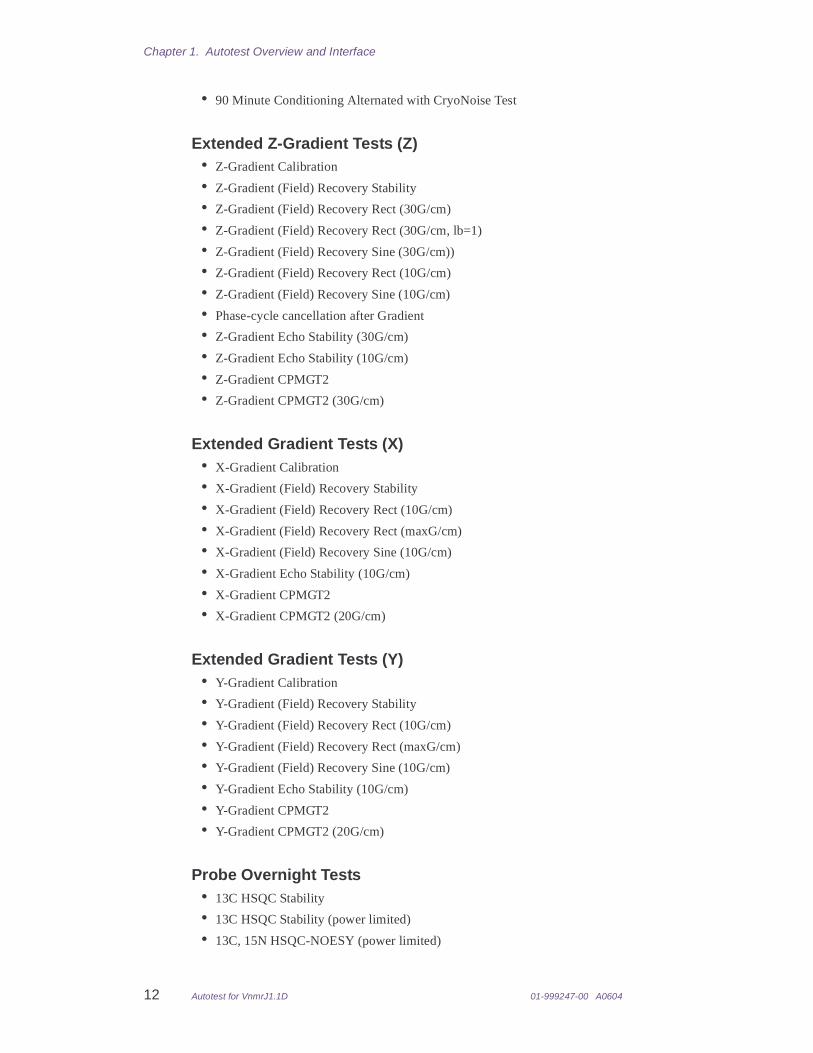
• “Extended Z-Gradient Tests (Z),” page 12

• “Extended Gradient Tests (X),” page 12

• “Extended Gradient Tests (Y),” page 12

• “Probe Overnight Tests,” page 12

• “N15 Tests (using channel 3 hardware - cable to N15 probe port),” page 13



• “N15 Tests (using channel 2 hardware - cable to N15 probe port),” page 13

• “AutoTest Sample with 100 mM NaCl,” page 13

• “AutoTest Sample with 250 mM NaCl,” page 13

• “Power-Limited 13C Pulse / Decoupling Tests (Channel 2: ~10msec 13Cpw90),” page 13

• “Probe Overnight Tests ( ~10msec 13Cpw90),” page 14

General• H1 RF Homogeneity

• High-Frequency Amplifier Compression

• T1 Determination

• Receiver Gain

• DSP Sensitivity Improvement

• Quadrature Image

• Spectral Purity Test

• Phase-Cycle Cancellation

• Phase-Cycle Cancellation vs. Recycle Time

• Spinlock Heating Test

• variable Temperature Test

• Lock Power and Gain Text

• Gradient Mapping and Shimming

• RF Field Mapping

2H Tests• 2H PW90 on Lock Coil (tn=lk)

• 2H Stability / Sensitivity (tn=lk)

• 2H spinlock Test (tn=lk)

• 2H PW90 on Lock Coil (Channel 3, Recable)

• 2H PW90 on Lock Coil (Channel 4, Recable)

• 2H Stability (Channel 4, Recable)

• 2H PW90 on Lock Coil (Lock / Decoupler, Recable)

• 2H Stability (Lock/Decoupler, Recable)

Channel 1• H1 pw90

• 90/10 Degree, 1µsec Pulse Stability / Sensitivity

• 30 Degree Pulse Stability

• Phase Stability

• Quadrature Phase Shift

• Small-Angle Phase Shift



• Pulse Turnon Time

• Dante Pulse Train

• Attenuator Test

• Linear Modulator Test

Channel 2• H1 pw90

• 90/10 Degree, 1µsec Pulse Stability / Sensitivity

• 30 Degree Pulse Stability

• Phase Stability

• Quadrature Phase Shift

• Small-Angle Phase Shift

• Pulse Turnon Time

• Dante Pulse Train

• Attenuator Test

• Linear Modulator Test

C13 Tests (Using channel 2 hardware - normal cabling)• C13 PW90 and Low-Band Amplifier Compression

• C13 RF Homogeneity

• C13 Phase Modulation Decoupling Profiles

• C13 Adiabatic Decoupling Profiles

• Methanol Amplitude Stability using 3kHz C13 Decoupling


• C13 Decoupling Heating Test

C13 Tests (Using channel 3 hardware - must re-cable)• C13 PW90 and Low-Band Amplifier Compression


• C13 Phase Modulation Decoupling Profiles



Shaped Pulses (channel 1)• Gaussian Pulse Excitation

• Gaussian 90 Degree Stability

• Gaussian Phase Stability

• GaussianSLP Phase Stability

• Gaussian Power / Pulse Width Array

• Rectangular vs. Gauss vs. EBURP1



• Pbox Shapes

• Shaped Pulse Amplitude Scaling

Shaped Pulses (channel 2)• Gaussian Pulse Excitation

• Gaussian 90 Degree Stability

• Gaussian Phase Stability

• GaussianSLP Phase Stability

• Gaussian Power / Pulse Width Array

• Rectangular vs. Gauss vs. EBURP1

• Pbox Shapes

• Shaped Pulse Amplitude Scaling

Standard Gradient Tests (Z) • Z-Gradient Calibration

• Z-Gradient (Field) Recovery Stability

• Z-Gradient (Field) Recovery Rect (30G/cm)

• Z-Gradient (Field) Recovery Sine (30G/cm)



• Phase-cycle cancellation after Gradient

• Z-Gradient Echo Stability (30G/cm)


• Z-Gradient CPMGT2

Standard Gradient Tests (X) • X-Gradient Calibration

• X-Gradient (Field) Recovery Stability

• X-Gradient (Field) Recovery Rect (10G/cm)

• X-Gradient (Field) Recovery Sine (10G/cm)

• X-Gradient Echo Stability (10G/cm)

• X-Gradient CPMGT2

Standard Gradient Tests (Y) • Y-Gradient Calibration

• Y-Gradient (Field) Recovery Stability

• Y-Gradient (Field) Recovery Rect (10G/cm)

• Y-Gradient (Field) Recovery Sine (10G/cm)

• Y-Gradient Echo Stability (10G/cm)

• Y-Gradient CPMGT2



Power-Limited 13C Pulse Tests (Channel 2)• C13 PW90 and LB Amplifier Compression


• C13 PW90 / Fine Power for 15.0 µsec 90

• C13 RF Homogeneity for 15.0 µsec 90

• C13 pw90 vs. power: Amplifier Linearity

Power-Limited 13C Pulse Tests (Channel 3)• C13 PW90 and LB Amplifier Compression


• C13 pw90 vs. power: Amplifier Linearity

Power-Limited C13/N15 Decoupling Efficiency Tests• C13 Phase Modulation Decoupling Profiles


• C13 WURST2 / WRUST40 Decoupling Profiles

• C13 Adiabatic, Waltz, No Decoupling 1D Comparisons

• C13 Decoupling 1D Comparisons

• C13 14kHz Adiabatic Decoupling Intensity / Linewidth Stability

• C13 6kHz Adiabatic Decoupling Intensity / Linewidth Stability

• C13 140ppm Adiabatic Decoupling Intensity / Linewidth Stability


• C13 Decoupling Line Broadening Test

Power-Limited 13C/N15 Decoupling Noise and Stability Tests• C13 / N15 Decoupling Noise in FID at max power

• C13 / N15 Decoupling Noise in FID vs. power



• H2O Amplitude Stability with 13C Decoupling

• H2O Amplitude Stability with 15N Decoupling

• H2O Amplitude Stability with 13C and 15N Decoupling

• H2O SN vs. C13 Decoupling Power

• H2O SN vs. C13 Decoupling Power (w/15N dec)

• H2O SN vs. N15 Decoupling Power

• H2O SN vs. N15 Decoupling Power (w/13C dec)

C13 N 15 Decoupling Installation Tests for Cryogenic Probe• 15 Minute Conditioning Alternated with CryoNoise Test

• 30 Minute Conditioning Alternated with CryoNoise Test



• 90 Minute Conditioning Alternated with CryoNoise Test

Extended Z-Gradient Tests (Z)• Z-Gradient Calibration

• Z-Gradient (Field) Recovery Stability


• Z-Gradient (Field) Recovery Rect (30G/cm, lb=1)

• Z-Gradient (Field) Recovery Sine (30G/cm))



• Phase-cycle cancellation after Gradient



• Z-Gradient CPMGT2

• Z-Gradient CPMGT2 (30G/cm)

Extended Gradient Tests (X)• X-Gradient Calibration

• X-Gradient (Field) Recovery Stability

• X-Gradient (Field) Recovery Rect (10G/cm)

• X-Gradient (Field) Recovery Rect (maxG/cm)

• X-Gradient (Field) Recovery Sine (10G/cm)

• X-Gradient Echo Stability (10G/cm)

• X-Gradient CPMGT2

• X-Gradient CPMGT2 (20G/cm)

Extended Gradient Tests (Y)• Y-Gradient Calibration

• Y-Gradient (Field) Recovery Stability

• Y-Gradient (Field) Recovery Rect (10G/cm)

• Y-Gradient (Field) Recovery Rect (maxG/cm)

• Y-Gradient (Field) Recovery Sine (10G/cm)

• Y-Gradient Echo Stability (10G/cm)

• Y-Gradient CPMGT2

• Y-Gradient CPMGT2 (20G/cm)

Probe Overnight Tests• 13C HSQC Stability

• 13C HSQC Stability (power limited)

• 13C, 15N HSQC-NOESY (power limited)



• 13C HSQC 1D vs. s2pul (power limited)

• Methanol HSQC Stability vs. 13C Pulse Power (coupled)

• Methanol HSQC Stability vs. 13C Pulse Power (decoupled)

• Methanol HSQC Stability vs. 13C Decoupling Power (decoupled)

N15 Tests (using channel 3 hardware - cable to N15 probe port)• N15 PW90 and Low-Band Amplifier Compression

• N15 HMQC Stability

• N15 pw90 vs. power: Amplifier Linearity

• N15 Decoupling Heating Test

• N15 Decoupling Heating Test with Power Limit

N15 Tests (using channel 2 hardware - cable to N15 probe port)• N15 PW90 and Low-Band Amplifier Compression

• N15 HMQC Stability

• N15 pw90 vs. power: Amplifier Linearity

• N15 Decoupling Heating Test

• N15 Decoupling Heating Test with Power Limit

AutoTest Sample with 100 mM NaCl• H1 RF Homogeneity (with 100mM NaCl)

• H1 pw90 (with 100mN NaCl)

• 90- and 10-Degree Stability and sensitivity (with 100 mM NaCl)



AutoTest Sample with 250 mM NaCl• H1 RF Homogeneity (with 250mM NaCl)

• H1 pw90 (with 100mN NaCl)

• 90- and 10-Degree Stability and sensitivity (with 250 mM NaCl)



Power-Limited 13C Pulse / Decoupling Tests (Channel 2: ~10µsec 13Cpw90)

• C13 PW90 and LB Amplifier Compression


• C13 PW90 for 10µsec 90

• C13 RF Homogeneity for 10µsec 90

• C13 pw90 vs. power: Amplitude Linearity






Probe Overnight Tests ( ~10µsec 13Cpw90)• 13C HSQC Stability ( ~10µsec 13Cpw90)

• 13C HSQC Stability ( ~10µsec 13Cpw90 power limited)

• 13C, 15N HSQC-NOESY ( ~10µsec 13Cpw90 power limited)

• 13C HSQC 1D vs. s2pul ( ~10µsec 13Cpw90 power limited)

• Methanol HSQC Stability vs. 13C Pulse Power (coupled)

• Methanol HSQC Stability vs. 13C Pulse Power (decoupled)

• Methanol HSQC Stability vs. 13C Decoupling Power (decoupled)

1.5 History TabSelecting the History tab at the top of the AutoTest window provides graphical output of the history files accumulated after several AutoTest runs.

To select a history file, scroll to the name of the file. The left arrow and right arrow may be used to rapidly step through the list.

Buttons are provided to specify a graphical or text output of the history file. If more than one result is contained in the history file, a menu of choices is displayed to the right of the display of results.

Values of results that exceed specified limits are displayed in red in the graphical output and in color in the text output. If a history file has multiple results with specifications, all displayed points for that run will indicate failure if only one has failed. Thus, a particular display may show a failure even though the result is within specification. If this is true, select the other entries in the list to show which result had actually failed.

Printed graphs may be obtained by selecting the button at the bottom of the screen. A full set of small graphs is plotted automatically after an AutoTest run when the Graph History check box is selected in the Configuration display (if automatic plotting is requested).

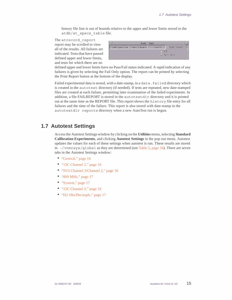
1.6 Test ReportSelecting the Test Report tab at the top of the AutoTest window allows viewing the atrecord_report file, a report on the results for the current AutoTest run. The atrecord_report file is one of two files that contain test results (both files are stored in the autotestdir directory):

• The REPORT file is more compact and is automatically printed at the end of the run.

• The atrecord_report has the same results, but in a format that is similar to the history file format. In addition, it indicates a Fail status if any of the results in a

1.7 Autotest Settings


history file line is out of bounds relative to the upper and lower limits stored in the atdb/at_specs_table file.

The atrecord_report report may be scrolled to view all of the results. All failures are indicated. Tests that have passed defined upper and lower limits, and tests for which there are no defined upper and lower limits have no Pass/Fail status indicated. A rapid indication of any failures is given by selecting the Fail Only option. The report can be printed by selecting the Print Report button at the bottom of the display.

Failed experimental data is stored, with a date-stamp, in a data.failed directory which is created in the autotest directory (if needed). If tests are repeated, new date-stamped files are created at each failure, permitting later examination of the failed experiments. In addition, a file FAILREPORT is stored in the autotestdir directory and it is printed out at the same time as the REPORT file. This report shows the history file entry for all failures and the time of the failure. This report is also stored with date-stamp in the autotestdir reports directory when a new AutoTest run is begun.

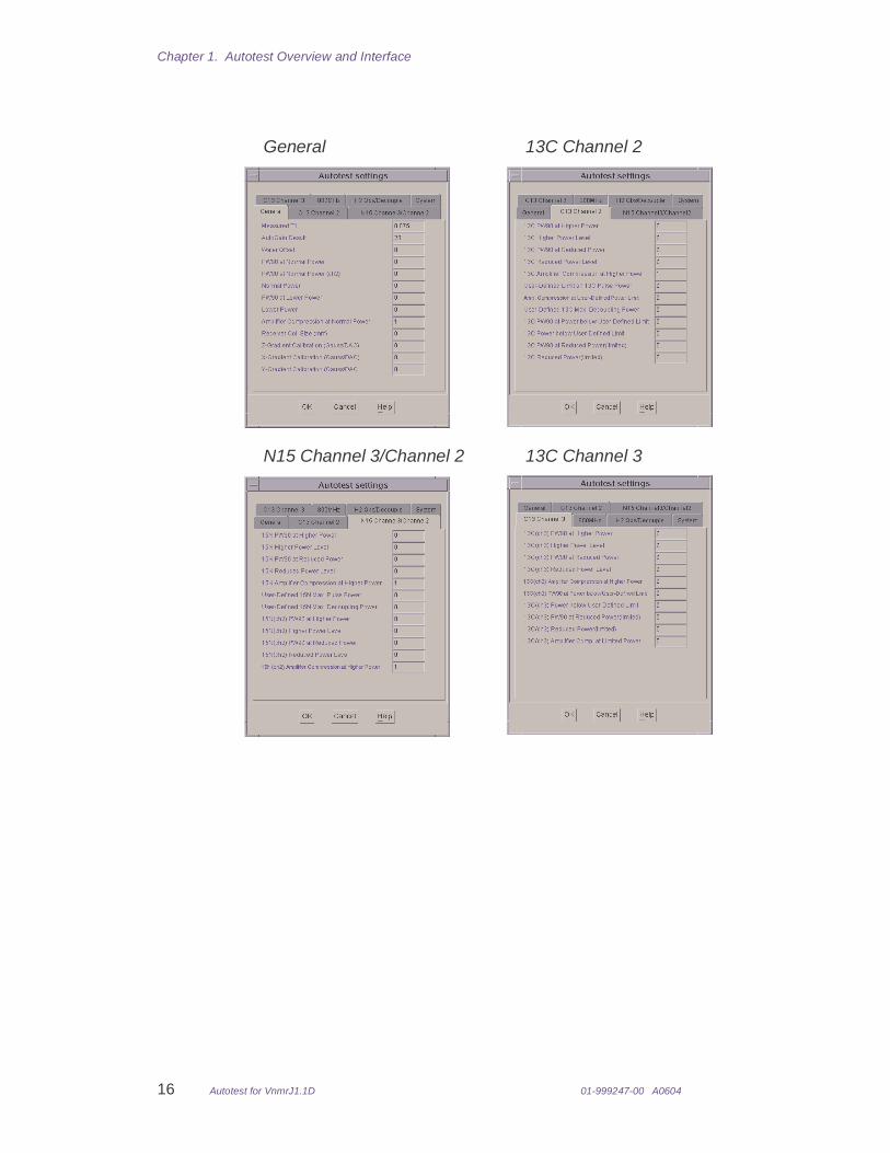
1.7 Autotest SettingsAccess the Autotest Settings window by clicking on the Utilities menu, selecting Standard Calibration Experiments, and clicking Autotest Settings in the pop out menu. Autotest updates the values for each of these settings when autotest is run. These results are stored in ~/vnmrsys/global as they are determined (see Table 2, page 34). There are seven tabs in the Autotest Settings window:

• “General,” page 16

• “13C Channel 2,” page 16

• “N15 Channel 3/Channel 2,” page 16

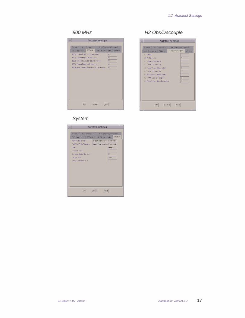
• “800 MHz,” page 17

• “System,” page 17

• “13C Channel 3,” page 16

• “H2 Obs/Decouple,” page 17



General 13C Channel 2

N15 Channel 3/Channel 2 13C Channel 3

1.7 Autotest Settings


800 MHz H2 Obs/Decouple

System


Chapter 2. Autotest - Operation

• 2.1 “Getting Started” this page

• 2.2 “AutoTest Setup” page 20

• 2.3 “Run Autotest” page 25

• 2.4 “Standard Tests Performed by AutoTest” page 25

2.1 Getting Started

AutoTest Sample

As the sample, AutoTest uses 0.1% 13C-enriched methanol in 1% H2O/99% D2O. More recent samples have 0.1% 15N-enriched acetonitrile added, as well. The sample is doped with gadolinium chloride at a concentration of 0.30 mg/ml, which produces a 1H T1 relaxation time of about 50 to 75 ms. The resulting line width is considerably larger than the magnet-determined line width because of the paramagnetic relaxation contribution, minimizing any dependence on shimming skill and permitting rapid collection of data.

Autotest for INOVA ATP and Running It the First Time

The INOVA ATP is run using a room temperature (not a cold probe) 5 mm Z-axis HCN probe.

The first time Autotest is run for a specific probe and console pair and for the INOVA ATP, the full set of ATP tests must be run.

Do the following:

• Follow the procedures in “AutoTest Setup” on this page

• Enable the typical and ATP outputs listed “Output Configuration” page 23

• Enable the typical and ATP tests listed in “Enable Tests,” page 23

• Select the test package ALL, see “Select Test Packages,” page 24

• Make a backup copy of the final ATP results.

System Set Up

1. Use the sample described in “AutoTest Sample,” page 19.

2. Set up all elements of the rf system (transmitters, linear modulators, rf attenuators, amplifiers, receivers, and probes) in their standard configuration.

3. Do the following if the system has a PFG (pulsed field gradients) accessory installed:



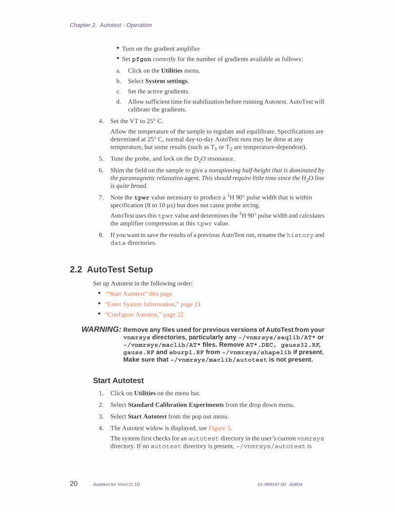
• Turn on the gradient amplifier

• Set pfgon correctly for the number of gradients available as follows:

a. Click on the Utilities menu.

b. Select System settings.

c. Set the active gradients.

d. Allow sufficient time for stabilization before running Autotest. AutoTest will calibrate the gradients.

4. Set the VT to 25° C.

Allow the temperature of the sample to regulate and equilibrate. Specifications are determined at 25° C, normal day-to-day AutoTest runs may be done at any temperature, but some results (such as T1 or T2 are temperature-dependent).

5. Tune the probe, and lock on the D2O resonance.

6. Shim the field on the sample to give a nonspinning half-height that is dominated by the paramagnetic relaxation agent. This should require little time since the H2O line is quite broad.

7. Note the tpwr value necessary to produce a 1H 90° pulse width that is within specification (8 to 10 µs) but does not cause probe arcing.

AutoTest uses this tpwr value and determines the 1H 90° pulse width and calculates the amplifier compression at this tpwr value.

8. If you want to save the results of a previous AutoTest run, rename the history and data directories.

2.2 AutoTest Setup Set up Autotest in the following order:

• “Start Autotest” this page

• “Enter System Information,” page 21

• “Configure Autotest,” page 22

WARNING: Remove any files used for previous versions of AutoTest from your vnmrsys directories, particularly any ~/vnmrsys/seqlib/AT* or ~/vnmrsys/maclib/AT* files. Remove AT*.DEC, gauss32.RF, gauss.RF and eburp1.RF from ~/vnmrsys/shapelib if present. Make sure that ~/vnmrsys/maclib/autotest is not present.

Start Autotest

1. Click on Utilities on the menu bar.

2. Select Standard Calibration Experiments from the drop down menu.

3. Select Start Autotest from the pop out menu.

4. The Autotest widow is displayed, see Figure 3.

The system first checks for an autotest directory in the user’s current vnmrsys directory. If no autotest directory is present, ~/vnmrsys/autotest is

2.2 AutoTest Setup


automatically created and subdirectories are copied from /vnmr/autotest. These directories include parameter, data, history and database atdb directories.

Enter System Information

At the top of the Configuration display see Figure 3, are fields for entering user, console, and probe identification as well as the nominal tpwr and pw90 values for 1H.

The tpwr and pw90 values are used as starting points and should be entered the first time AutoTest is run. The 1H pw90 value should be correct to within ±30%. The power level entered is used for most of the tests so it should be a level that is used in normal day-to-day work. For most probes this would be a power level sufficient to get a 10 µs pw90.

Running at the upper range of tpwr may result in a situation where the amplifier is in compression. This means that although the pw90 may be shorter at tpwr=63 than tpwr=57, the pw90 at the former power may not be a factor of two shorter. If a 100-watt high-frequency amplifier is present, the tpwr value should be set so that 1H pw90 is 10 µs at that power. In any case, the amplifier compression at the entered tpwr is determined, with the assumption that tpwr-12 dB is a setting where there is linear behavior.

The length (in mm) of the active window in the receiver coil is also specified. This is normally 16 mm, unless the probe has a hexagonal base (Unibody-style), in which case the coil may have an 18 mm length (normally true for indirect and triple-resonance liquids probes).

Some probes (very high field and cryogenic) require more careful power control. Power control for 13C and 15N pulses and decoupling is available within this panel. These values are used to set upper limits on power (attenuator) settings for 13C and 15N (using channels 2 and 3) pulses and decoupling for those tests which have power limits. These are primarily

Figure 3. Autotest Configuration Window



Configure Autotest

System information fields



decoupling noise tests. The 13C pw90 calibration is normally done for a power level giving a nominal 15 µsec pulse and this power level is found by experiment. This power value is limited by the above values if the tests are labeled “power limited”. If the probe used has no 15N port, set the maximum pulse power to zero. The relevant macros check for a zero value and skip 15N pulses or decoupling for this case. AutoTest macros including c after AT have power limits internally coded.

Enter the following information their respective data fields:

Configure Autotest

Below the system information entry fields are check boxes for configuring the output and enabling various tests, see Figure 3. Configure Autotest in the following order:

• “Output Configuration” on this page

• “Enable Tests,” page 23

• “Select Test Packages,” page 24

Field Label Field Description

Operator Name: Field will automatically be filled in using the log in name of the current UNIX user that has started VnmrJ. If a different name is desired, type in the desired operator name.

Console type: Enter a description of the console type, e.g. INOVA 500.

Console S/N: Enter the console serial number.

Data Directory: Accept the default data path or provide an alternate path, beginning with root (/).

Probe: Enter a description of the probe or use the probe’s serial number.

Coil size (mm): Enter the coil size if the probe is equipped with a gradient or gradients coil.

Max 13C Pulse Power: Enter the maximum power (attentuator settings) for any 13C pulse.

Max 13C Dec. Power: Enter the maximum power (attentuator setting) for any 13C decoupling.

Max 15N Pulse Power: Enter the maximum power (attentuator settings) for any 15N pulse.

Max 15N Pulse Power: Enter the maximum power (attentuator setting) for any15N decoupling,

1H Pulse Power: Enter a tpwr for a nominal 1H pw90 of 10 µsec.

Nominal 1H pw90: Enter a nominal 1H pw90 at the above power.

2.2 AutoTest Setup


Output Configuration

Checkboxes for configuring the output are

These checkboxes reflect the setting (y or n) of global parameters at_plotauto, at_plotparams, at_graphs, and at_wntproc, respectively. These global parameters, as well as those mentioned for test selection, are updated when the Begin Test button is selected.

Note: If you select Auto Plotting, Print Parameters, or Graph History, make sure enough paper is available for the printer or plotter.

Enable Tests

The checkboxes on the AutoTest window set whether VT, 13C, lock, and gradient tests are enabled or not. These check boxes should be set appropriately before selecting the Begin Test button. If these are not selected, any tests involving them are skipped in an AutoTest run, even if the tests are selected in a test package or individually.

The normal use of these check boxes is to allow skipping of some tests when the All Standard Tests package is used. The boxes reflect the current state of the options when the AutoTest program starts (these boxes reflect the user global parameters values, y or n, of at_vttest, at_c13tests, at_locktests, and at_gradtests, respectively).

In most cases, a single AutoTest run is appropriate and the Repeat Until Stopped checkbox should not be set. For troubleshooting, or to establish a statistically valid database,

OptionTypical and ATP Setting

Description

Auto Plotting Enabled Automatic plotting of spectra after each experiment. This box should be on the first time AutoTest is run to produce a hardcopy record, but can be off for subsequent normal maintenance mode.

Print Parameters Enabled Automatic plotting of a separate page that includes a parameter set, pulse sequence and descriptive text (only if Auto Plotting is selected). This box should be on the first time AutoTest is run to produce a hardcopy record, but can be off for subsequent normal maintenance mode.

Graph History Enabled Automatic plotting of history graphs (only if Auto Plotting is selected).

Process During Acq.

Enabled Automatic (wnt) processing and display of spectra after each FID.

OptionTypical and ATP Setting

Description

Enable VT test Enabled Tests the VT if the hardware is present and the probe supports VT operations.

Enable C13 tests Enabled Tests 13C related instrument and probe performance.

Enable Lock tests Enabled Tests lock functions and stability

Enable Gradient tests Enabled Test gradient hardware and probe.

Repeat Until Stopped Disabled Automatic repeating of AutoTest (until manually aborted).



however, you might want to run the test overnight. When the Repeat Until Stopped checkbox is selected, the automatic processing and display of data after each FID option is disabled after the first pass (because it is unlikely that the user is present to view the data). In addition, all function tests that do not produce a numerical result are skipped. This check box sets the global parameter at_cycletest.

Select Test Packages

In the center of the AutoTest window is a column of check boxes used to select test package, see Figure 3 and Figure 4.

The first checkbox is All Standard Tests. This option sets AutoTest to make a full run, checking out all the relevant hardware enabled by the upper checkboxes.

All Standard Tests must be the first test performed (with all options enabled) because it determines calibrations for any of the specific tests and is required for the INOVA ATP.

Click the check boxes next to each output and test options that are to be used or click the check box next to All Standard Tests or All Standard Tests (Power Limited) to select the standard test array.

The list of test spans two pages, see Figure 3 for page 1 of the tests and Figure 4 for page 2 of the tests. Click on the arrows to move between pages.

Once the full AutoTest is run, any single test may be run and it uses the calibrations stored in the standard parameter set or in the global variables updated by specific tests. Thus, a single test can be run without doing any calibrations, but its accuracy is dependent on the last calibration performed.

As AutoTest experiments are completed, relevant calibrations are stored in special global parameters (Table 2, page 34). In addition, the standard.par parameter set (stored in autotestdir+/parameters) is updated whenever the tof, pw90, T1, linewidth, or gain values are determined. These are determined in the first few experiments of the All Standard Tests run, or if specific tests are requested.

Thus, if only a single specific test is requested, the standard.par parameters should have appropriate values so that a full autocalibration of all parameters is unnecessary. The relevant global parameters include C13-related parameters, gradient calibrations, etc. The macro /vnmr/maclib/maclib.autotest/ATglobal creates these variables (if not already present) and you can read it to get an idea of the global variables used by AutoTest. For VnmrJ, the utilities, menu has AutoTest information showing the values of most of the AutoTest global parameters.

Below the All Standard Tests checkbox are several checkboxes for different packages of tests. By selecting one or more of these, you can chose the tests performed. Selections may be unselected by clicking the checkbox once again.

If there is not enough room within the display to show all choices, a pair of arrow symbols appears at the top of the list. Selecting the right arrow updates the display with the next list of choices. Selecting the left arrow returns to the previous page of choices.



Figure 4. Autotest Configuration Test List Page 2

2.3 Run Autotest


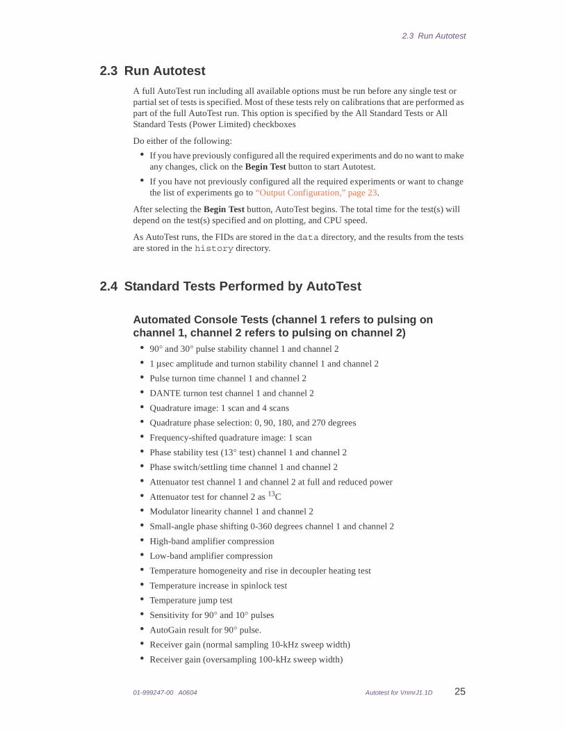
2.3 Run AutotestA full AutoTest run including all available options must be run before any single test or partial set of tests is specified. Most of these tests rely on calibrations that are performed as part of the full AutoTest run. This option is specified by the All Standard Tests or All Standard Tests (Power Limited) checkboxes

Do either of the following:

• If you have previously configured all the required experiments and do no want to make any changes, click on the Begin Test button to start Autotest.

• If you have not previously configured all the required experiments or want to change the list of experiments go to “Output Configuration,” page 23.

After selecting the Begin Test button, AutoTest begins. The total time for the test(s) will depend on the test(s) specified and on plotting, and CPU speed.

As AutoTest runs, the FIDs are stored in the data directory, and the results from the tests are stored in the history directory.

2.4 Standard Tests Performed by AutoTest

Automated Console Tests (channel 1 refers to pulsing on channel 1, channel 2 refers to pulsing on channel 2)

• 90° and 30° pulse stability channel 1 and channel 2

• 1 µsec amplitude and turnon stability channel 1 and channel 2

• Pulse turnon time channel 1 and channel 2

• DANTE turnon test channel 1 and channel 2

• Quadrature image: 1 scan and 4 scans

• Quadrature phase selection: 0, 90, 180, and 270 degrees

• Frequency-shifted quadrature image: 1 scan

• Phase stability test (13° test) channel 1 and channel 2

• Phase switch/settling time channel 1 and channel 2

• Attenuator test channel 1 and channel 2 at full and reduced power

• Attenuator test for channel 2 as 13C

• Modulator linearity channel 1 and channel 2

• Small-angle phase shifting 0-360 degrees channel 1 and channel 2

• High-band amplifier compression

• Low-band amplifier compression

• Temperature homogeneity and rise in decoupler heating test

• Temperature increase in spinlock test

• Temperature jump test

• Sensitivity for 90° and 10° pulses

• AutoGain result for 90° pulse.

• Receiver gain (normal sampling 10-kHz sweep width)

• Receiver gain (oversampling 100-kHz sweep width)



• Folded noise reduction with large spectral width

• Benefit of oversampling at normal gain

• Benefit of oversampling at normal gain + 12dB

• Signal-to-noise as function of gain

• Spectral purity (“glitch test”)

• Lock power test correlation coefficient

• Lock gain test correlation coefficient

Automated Tests with Shaped RF• Gaussian 90° stability, channel 1 and channel 2

• Gaussian phase stability test, channel 1 and channel 2

• Phase-ramped Gaussian phase stability test, channel 1 and channel 2

• Shaped pulse accuracy- gaussian excitation profile, channel 1 and channel 2

• RF amplitude predictability using a gaussian pulse at variable power, channel 1 and channel 2

• RF amplitude predictability using a gaussian, rectangular and eburp-1 pulses, channel 1 and channel 2

• Amplitude scaling of shaped pulses using a gaussian pulse, channel 1 and channel 2

• RF excitation predictability using a variety of shaped pulses, channel 1 and channel 2

Automated Decoupling Performance Tests• 13C phase modulation decoupling profiles

13C GARP decoupling profile13C WALTZ-16 decoupling profile13C XY-32 decoupling profile13C MLEV-16 decoupling profile

• 13C adiabatic decoupling profiles (if waveform generator present on decoupling channel):13C STUD decoupling profile13C WURST decoupling profile

• Sample heating during 13C broadband decoupling

Automated 90° Pulse Width Calibrations (PW90)• 1H 90° pulse width calibrations on channels 1 and 2 at high and reduced power

• 13C 90° pulse width calibrations at high and reduced power

RF Homogeneity Tests• 1H rf homogeneity test

• 13C rf homogeneity test

2.4 Standard Tests Performed by AutoTest


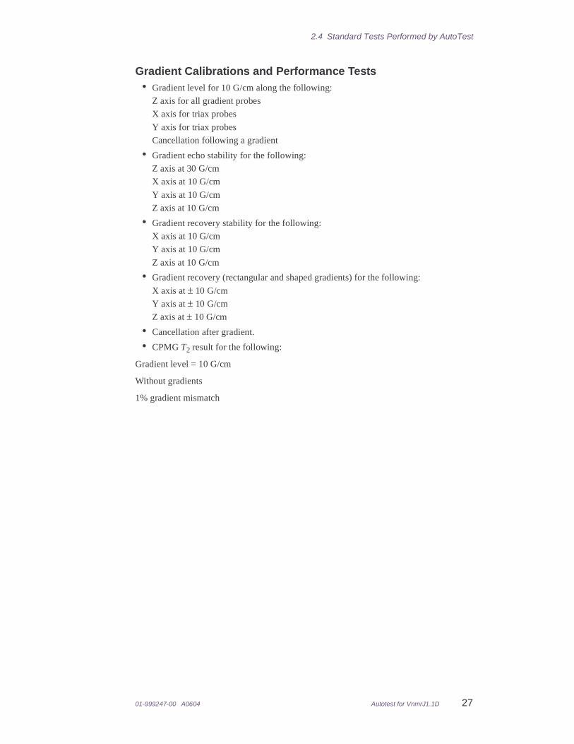
Gradient Calibrations and Performance Tests• Gradient level for 10 G/cm along the following:

Z axis for all gradient probes

X axis for triax probes

Y axis for triax probes

Cancellation following a gradient

• Gradient echo stability for the following:

Z axis at 30 G/cm

X axis at 10 G/cm

Y axis at 10 G/cm

Z axis at 10 G/cm

• Gradient recovery stability for the following:

X axis at 10 G/cm

Y axis at 10 G/cm

Z axis at 10 G/cm

• Gradient recovery (rectangular and shaped gradients) for the following:

X axis at ± 10 G/cm

Y axis at ± 10 G/cm

Z axis at ± 10 G/cm

• Cancellation after gradient.

• CPMG T2 result for the following:

Gradient level = 10 G/cm

Without gradients

1% gradient mismatch


Chapter 3. Autotest - Administration

• 3.1 “Saving Data and FID Files from Previous Runs,” page 29

• 3.2 “Creating Probe-Specific Files,” page 29

• 3.3 “AutoTest Directory Structure,” page 30

• 3.4 “AutoTest Macros,” page 33

3.1 Saving Data and FID Files from Previous RunsAs AutoTest executes, data and FID files are written into the history and data directories, which are located in the autotest directory. The autotest directory is usually located in the directory vnmrsys of a user’s home directory. The contents of the data directory are progressively overwritten as AutoTest continues.

Before starting a new AutoTest run, do the following to save the data from a previous run:

1. Open a UNIX window. and enter cd ~/vnmrsys/autotest.

2. Change the name of the history directory by entering, for example,mv history history.old.

3. Change the name of the data directory by entering, for example, mv data data.old

3.2 Creating Probe-Specific FilesIf you run AutoTest with different probes, you should keep separate autotest directories. Use the following steps to create probe-specific files.

1. After you have run AutoTest using a specific probe, change the name of the autotest directory by using the mv command, for example:cd ~/vnmrsysmv autotest autotest_probe_1

Where probe_1 is the name of the probe that was tested, for example, 5mmTriplePFG or 5mmID.

Any new AutoTest run automatically creates a new autotest directory in the user’s vnmrsys directory. The only file that needs to be updated would be~/vnmrsys/autotest/parameters/standard.par. This can either be copied from the saved autotest file or the parameter set may be retrieved using rt or rtp, the parameters updated and then saved, replacing the standard.par file. This should be safe for any parameters displayed in the dg window, but there are several parameters dealing with gradients and indirect detection that must also be checked. It is safest to do an All Standard Tests run the first time a new probe is used.



Once a calibrated standard.par parameter set is present, autotest directories may be renamed whenever a probe is changed. In this way, history files may be kept specific to a probe.

2. To change the file name back to probe_1 (or the name you have chosen), enter, for example:cd ~vnmrsysmv autotest autotest_probe_2

Where probe_2 is the name you have chosen for the probe last tested.mv autotest_probe_1 autotest

Where probe_1 is the name you have chosen for the probe you now want to test.

If you need to repeat any individual test, you can do so by recalling the appropriate FID from the data directory. The experiment can then be started with the go command without overwriting the previous data. Or the test may be selected from the Test Library after using the autotest macro or a menu calling this macro.

3.3 AutoTest Directory StructureAutoTest uses the ~/vnmrsys/autotest directories listed in Table 1.

data Directory

The ~/vnmrsys/autotest/data directory contains FIDs collected in previous AutoTest experiments. As each experiment finishes, the macro specified by the wexp parameter executes, and as part of that macro, a svf command is performed that saves the FID under a file name specified by the parameter at_currenttest (if it contains a name). The macro first removes any file by the same name (the results of the test from the last time it was run) and then executes svf. Thus, the data directory may contain FIDs obtained during different AutoTest runs if those runs were not full runs.

Any data files stored in the data directory can be recalled by normal VNMR commands such as rt. The data may then be transformed and displayed. The wexp parameter will contain the name of the macro normally used for data processing, so that the wexp command can be used to duplicate the actions normally done in an automatic manner.

Note: If file ~/vnmrsys/autotest/atdb/at_selected_tests is empty, only processing and no further acquisition is done. If the file ~/vnmrsys/autotest/atdb/at_cycled_tests is not empty, those tests may start.

Table 1. AutoTest Directories.

Directory Contents

data FIDs from the recent AutoTest run(s)

data.failed FIDs from any failed Auto Test experiments

history History files for the various tests

reports Copies of the report generated each time AutoTest is run

parameters Parameter files—default entry is standard.par

texts Copies of the text files attached to the AutoTest experiments

atdb AutoTest database

3.3 AutoTest Directory Structure


Therefore, clear the contents of at_selected_tests and at_cycled_tests before manually executing the macro.

This result is normally the case if the last AutoTest run came to a normal completion. However, if the last AutoTest run was aborted and no new entry into the AutoTest Program was done, this file will contain entries and an acquisition may start up following the wexp command. If so, just abort the acquisition.

data.failed Directory

The ~/vnmrsys/autotest/data.failed directory contains any data from any failed experiment. Failure results when a calculated result falls outside limits defined in the ~/vnmrsys/autotest/atdb/at_spec_table file. Varian specifications are indicated in the ~/vnmrsys/autotest/atdb/at_spec_table file. Users can modify this file by supplying upper and lower limits. Any user-modified at_spec_table file should be backed up outside ~/vnmrsys/autotest, since this file can be deleted later.

parameters Directory

The ~/vnmrsys/autotest/parameters directory contains any parameter set used by AutoTest macros, including any put there by the user. Normally, only standard.par is present. This parameter set has all parameters necessary for the AutoTest macros. Values of parameters may be displayed by using dg in the text window. Some parameters are only displayed when certain variables are nonzero, or 'y' if a string parameter; however, these parameters are printed and displayed if used in an experiment. The AutoTest macro ATrtp is used to recall a parameter set from this directory.

reports Directory

The ~/vnmrsys/autotest/reports directory contains text files from previous AutoTest runs, by date. Each run produces a report, whether plotting is requested or not. The report file for a currently proceeding AutoTest run is ~/vnmrsys/autotest/REPORT. At the end of an AutoTest run, this file is copied to the reports directory under a title that includes the date and time. If AutoTest is repeated, a new report is automatically written out for each complete AutoTest run. The existing ~/vnmrsys/autotest/REPORT file is renamed as ~/vnmrsys/autotest/LASTREPORT whenever an AutoTest run begins. Similar actions are executed for the atrecord_report. This directory also stores any FAILREPORTs with appropriate date-stamps.

texts Directory

The ~/vnmrsys/autotest/texts directory contains mainly text files that are printed on some spectral plots and most parameter set printouts. These files explain the purpose of the test.

history Directory

The ~/vnmrsys/autotest/history directory contains text files that record the values determined in AutoTest runs. They are generated automatically by the ATrecord macro which is used in any AutoTest macro that obtains a numerical result from an NMR experiment. Each result is written on a new line and is date-stamped. Tests that have a



Varian specification listed in the manual Acceptance Test Procedures will be denoted as having passed or failed.

If the history file has more than one result per line, any one failure will cause a fail result for the whole line. When the history file is viewed using the History display (after using the macro autotest), failure is indicated by a red data point in graphical output and a colored entry in the text output.

If a user writes a new AutoTest macro including the ATrecord macro, the at_spec_table must be updated for the history files to be displayed. In addition, the new macro must be listed within the at_tests_file.

atdb Directory

The ~/vnmrsys/autotest/atdb directory contains mainly the following text files used by the Auto Test program to create the AutoTest interface:

at_tests_file

The at_tests_file file defines all the tests that AutoTest can perform. Tests are specified by a macro name and description. Normally, these are grouped and separated by a line starting with Label. The word following will be displayed as a heading for a group of tests. The test descriptions are displayed in the Test Library display (after entering the macro autotest or by using a menu calling this macro). The macro names are not shown in the display, just checkboxes next to the test description.

New tests may be added to the at_tests_file by specifying a group title (use the Label keyword as the first word on the line, followed by a descriptive phrase). Specify a macro name and then a test description, one per line.

at_groups_file

The at_groups_file file defines test packages that have been assembled for convenience. Each package has a line that gives a description (in double quotes) followed by a list of macros to be used in the order of acquisition. There are no restrictions on the placement of these macros in the text file, only the order matters. When the next double-quoted entry appears, a new group is set.

The AutoTest interface display shows these packages as checkbox entries in the Configuration display. Selection of one or more of these causes their execution in the order of selection, once the Begin Test button is selected. When this happens, the at_selected_tests file is fixed. Selection of the All Standard Tests checkbox disables any other selections that will be done as part of the All Standard Tests run.

Users may add new packages to the Configuration display list by adding appropriate lines to the at_groups_file in the same format.

Any macro specified within a group must be defined in the at_tests_file.

at_selected_tests

The at_selected_tests file contains the names of the macros to be run as part of the AutoTest procedure and is fixed at the time the Begin Test button is selected. The format is one line per macro with each line containing the name of a macro, in the order of acquisition.

3.4 AutoTest Macros


As AutoTest proceeds, each line is deleted as the specified macro finishes its activity. Thus, completion of the AutoTest run is defined as when this file is empty. The single exception is the case of automatic repeating of AutoTest, as specified by the Repeat Until Stopped checkbox in the Configuration display and as indicated by the value of the global parameter at_cycletest('y'). In this case, at the completion of the AutoTest run, the contents of the file at_cycled_tests are copied into at_selected_tests and the process then continues.

at_cycled_tests

The at_cycled_tests file is updated when the Begin Test button is selected. If the Repeat Until Stopped checkbox is selected in the Configuration display, the global parameter at_cycletests is set to 'y' and the file at_selected_tests is copied to at_cycled_tests. If no test cycling is requested, this file is emptied.

at_spec_table

The at_spec_table file is written out when the ~/vnmrsys/autotest directory is created and is spectrometer-dependent. The appropriate file is copied from the directory /vnmr/autotest, depending on spectrometer frequency. It contains a list of macros used in AutoTest for producing entries in the history files. For each macro the following is specified:

• The history file affected by the macro.

• The column number (not counting date) containing the result.

• The lower limit for the result.

• The upper limit for the result.

• A text description of the result. This text description is used for the graphical displays and plots. A comment line above each macro serves to describe the test.

All results specified in the manual Acceptance Test Procedures have upper and lower limits specified numerically in this file. Those not having Varian specifications have asterisks (*) as entries for upper and lower limits and these results will have no indication of pass or fail in their history files, or colored indication of failure in the graphical displays of the history files.

Users may wish to set their own upper and lower limits for many, if not all, of the results. They may do so by replacing the asterisks with numbers. Of course, this should only be done after a good statistical base is obtained, such as more than 20 complete AutoTest runs. Once this base is obtained, the numbers put into the at_spec_table file should have a reasonable margin of error built in.

It is a good idea to make a copy of the file at_specs_table file prior to changing it, as well as the modified file, because deletion or renaming of the autotest directory will result in a default at_spec_table being copied from /vnmr/autotest/atdb.

3.4 AutoTest MacrosTo help users who want to add or modify tests, this section describes some of the macros used by AutoTest. These macros are in /vnmr/maclib/maclib.autotest.



ATglobal Macro

The ATglobal macro is run when the AutoTest program begins. The macro checks for the existence of autotest parameters in the user file ~/vnmrsys/global. These parameters are used to store calibrations and results that are used by autotest macros. If the parameters are not present, ATglobal creates them. Otherwise, the parameters are left unchanged. In VNMRJ, the Utilities drop-down menu system settings option permits convenient viewing (and entry of) AutoTest global parameters. A partial list of these parameters is given in Table 2.

Table 2. Selected Parameters Created by ATglobal

Parameter Contains

at_currenttest Name under which the FID is stored

autotestdir Full path of the autotest directory

at_user Name of the user running autotest (printed in report)

at_coilsize length (in mm) of active window in coil (typically 16 or 18 mm)

at_consoletype Name of console entered in AutoTest window

at_consolesn Number of console entered in AutoTest window

at_probetype Name entered for probe used in AutoTest window

at_wntproc y or n (for processing/display after each FID)

at_cycletest y or n (for automatic repeating of AutoTest)

at_printparams y or n (for parameter list/pulse sequence printouts)

at_plotauto y or n (for automatic plotting)

at_graphhist y or n (for history graphs plotting)

at_locktests y or n (for lock power/gain tests)

at_max_pwxlvl Maximum permitted 13C power level

at_max_pwx2lvl Maximum permitted 15N power level

at_max_dpwr Maximum permitted 13C decoupling power

at_max_dpwr2 Maximum permitted 15N decoupling power

at_T1 Value of last determined T1

at_gain Value of gain determined by autogain

at_tof Value of tof for water

at_fsq Value of fsq parameter

at_dsp Current value of dsp at start of run

at_ampl_compr Value of high-band amplifier compression

at_LBampl_compr Value of low-band amplifier compression

at_LBampl_compr_10usec_c 13C amp compression at at_pwx90lvl_10µsec_c

at_decHeating Temperature increase from decoupling

at_linewidth Linewidth of water resonance

at_pw90 90° pw at power specified in AutoTest display

at_tpwr Power specified in AutoTest display

at_pwx90c 13C pw90 at power at_pwx90lvlc

at_pwx90lvlc 13C power level for ~15-µs pwx90 at power<= to at_max_pwxlvl

at_pw90Lowpower 90° pw at reduced power

at_pwx90Lowpowerc 13C pw90 at power at_pwx90Lowpowerlvlc

at_tpwrLowpower Power level at reduced power

3.4 AutoTest Macros


ATstart Macro

The ATstart macro is run after the Begin Test button is selected in the Configuration display. The macro sets the global parameters to reflect the current state of the hardware and aborts under certain circumstances, such as if requested tests are not compatible with the current hardware settings.

Messages are displayed indicating the source of the problem. The reports are initialized with relevant information and the ATnext macro is executed.

ATnext Macro

The ATnext macro checks the at_selected_tests file and copies the first entry into the global parameter at_cur_smacro, deletes the top line in at_selected_tests and executes the macro specified by at_cur_smacro. If the at_selected_tests file is empty, ATnext either finishes the AutoTest run or calls the ATrestart macro which copies the at_cycled_tests file to at_selected_tests, permitting repeated AutoTest runs until manually aborted by the user.

ATnext is usually found at the bottom of each macro defining a particular test. This permits the linking of one test to another, in a general fashion.

ATxxx Macros

Specific tests usually have the designation of AT, followed by a number or group of letters. Each macro is self-contained, having the ability of setting up parameters, performing

at_pw90_ch2 90° pw on channel 2

at_pwx90 13C pw90 determined at at_pwx90lvl

at_pwx90lvl 13C power level for approximately 15-µs pwx90

at_pwx90Lowpower 13C pw90 at reduced power

at_pwx90Lowpowerlvl 13C power level at reduced power

at_pwx90_10usec_c 13C pw90 at power level at_pwx90lvl_10µsec_c

at_pwx90lvl_10usec_c 13C power level for ~10-µs pwx90 at power<= to at_max_pwxlvl(typically at 800 MHz)

at_pwx90Lowpower_10usec_c 13C pw90 at at_pwx90Lowpowerlvl_10µsec_c

at_pwx90Lowpowerlvl_10usec_c 13C power level for at_pwx90Lowpower_10usec_c

at_vttest y or n (for VT test)

at_temp Current temperature

at_vttype Current value of global parameter vttype

at_tempcontrol Value reflects usage of temp tcl/tk panel

at_gradtests y or n (for gradient tests)

at_pfgon Current value of pfgon

at_gmap y or n (for gradient mapping/shimming)

at_gzcal Value of G/cm per DAC unit for z-axis gradient

at_gxcal Value of G/cm per DAC unit for x-axis gradient

at_gycal Value of G/cm per DAC unit for y-axis gradient

Table 2. Selected Parameters Created by ATglobal

Parameter Contains



acquisition, processing the acquired data, possibly setting up new experiments and processing the data acquired from those experiments, creating plots, parameter printouts, archiving the raw data, performing statistical analyses of the data, and writing results to history files and reports.

To better illustrate the structure of these macros, Table 3 gives the source code for macro AT16, the turn-on test (channel 1). A column of descriptive comments has been added to clarify the statements.

ATcxxx Macros

ATcxxx macros use the 13C and 15N power limits.

ATrecord Macro

The ATrecord macro is run whenever a numerical result is stored in a history file. It is a general macro that will create the specified history file if it is not present. The macro has a minimum of four arguments: Name of history file, comment line, column header line (name of result) and value of result. For example, see the above macro near the bottom. The variables $turnon and $corrcoef are calculated prior to using the ATrecord macro, and these appear in two columns headed by time and corr_coef. Note the use of trunc. This is necessary to limit the number of decimal places produced.

Up to seven results may be stored in one history file. If this macro is used, be sure to modify the at_spec_file in ~/vnmrsys/autotest/atdb to add the necessary number of lines describing the results and any upper and lower limits desired. If a new history file fails to appear it is usually because of failure to update the at_spec_file. A backup copy should be made of the atdb in case of accidental overwriting.

The AutoTest macros can be run as independent macros if a specific test is desired. This is done by either entering the macro in the VNMR command line or by selecting the single test from the AutoTest test library panel by using a checkbox and the Begin button. Again, if the file at_selected_tests is not empty, the ATnext macro will start a new acquisition.

3.4 AutoTest Macros


Table 3. Source Code for AT16 Macro Example

if ($#=0) then First time AT16 is run it has no arguments.

ATrtp('standard') Recalls standard parameter set.

text('Pulse Turnon Test')

at_currenttest=turnon_ch1 Puts name of test in global variable.

tpwr=tpwr-6 ph

array('pw',37,0.1,.025) Sets up pulse width array.

ss=2

wnt='ATwft select(celem) aph0 vsadj dssh dtext' Specifies what to do every FID

wexp='AT16(`PART1`)' Specifies what to do at end of experiment.

ATcycle Disables wnt processing if in repeat mode.

au Begins acquisition and specifies wnt/wexp processing to occur.

write('line3','Pulse Turnon Test (channel 1)')

dps

elseif ($1='PART1') then This part executes at end of experiment.

if (at_plotauto='y') then

if (at_printparams='y') then

pap ATpltext If parameter printout requested.

pps(120,0,wcmax-120,90)

page

endif

endif

select(arraydim) aph0

f peak:$ht,cr rl(0) sp=-1p wp=2p vsadj dssh dtext

ATreg6 Fits to straight line and displays/plots data.

ATpl3:$turnon,$corrcoef Determines turn-on time and correlation coefficients

$turnon=trunc($turnon) $corrcoef= trunc(1000*$corrcoef)/1000

Limits number of decimal places.

ATrecord('TURNONch1','Pulse Turnon Time (nsec)(channel 1)','time ',$turnon,'corr_coef.',$corrcoef)

Writes out results to history file.

write('file',autotestdir+'/REPORT','Pulse Turnon Time (channel 1): %2.0f nsec.-Corr. Coef. = %1.3f ',$turnon,$corrcoef)

Writes results to report.

if (at_plotauto='y') then

ATpltext(100,wc2max-5)

full wc=50 pexpl page Plots regression fit

endif

ATsvf Removes old data set and stores FID under name in at_currenttest.

ATnext Starts next macro in at_selected_tests file, if present.

endif Closes elseif part


Chapter 4. Autotest - Test Reference

The sections in this chapter provide descriptions of the Autotest experiments.

• 4.1 “RF Performance Test Descriptions (Nonshaped Channels 1 and 2)” this page

• 4.2 “Shaped Pulse Test Descriptions (Channels 1 and 2)” page 45

• 4.3 “13C Test Descriptions” page 47

• 4.4 “Gradient Tests Descriptions” page 48

• 4.5 “CPMG T2” page 49

• 4.6 “13C Power-Limited Pulse Tests” page 50

• 4.7 “13C/15N Power-Limited Decoupling Tests” page 52

• 4.8 “15N Power-Limited Pulse and Decoupling Tests” page 57

• 4.9 “2H Pulse and Decoupling Tests” page 58

• 4.10 “Installation Tests for Cryogenic Probes” page 60

• 4.11 “Other Test Descriptions” page 61

• 4.12 “Tests Using Salty Sample” page 62

All units of the rf system (transmitters, linear modulators, rf attenuators, amplifiers, receivers, and probes) must be in the standard configuration when AutoTest is run. If the system configuration has been changed, it must be returned to the standard configuration before running AutoTest for acceptance testing.

All data is stored, and both plots and statistical analyses are provided as part of the acceptance testing. Plots and statistical analyses are made concurrently with acquisition.

4.1 RF Performance Test Descriptions (Nonshaped Channels 1 and 2)

This test group consists of the following tests:

• “Pulse Stability and Sensitivity” page 40

• “Cancellation Test” page 40

• “Phase Stability (13 deg. Phase Error) Test” page 41

• “Pulse Turn-on Time” page 41

• “Attenuator Linearity” page 41

• “Attenuator Linearity at Reduced Power” page 42

• “Linear Modulator Linearity Tests” page 42

• “Linear Modulator Linearity Tests with Attenuators Set to Full Attenuation” page 42

• “Pulse Shape Test—DANTE” page 42



• “Phase Switch Settling Time” page 43

• “RF Homogeneity” page 43

• “Receiver Test” page 44

• “Image Rejection Test” page 44

• “Quadrature Phase Selection” page 44

Pulse Stability and Sensitivity

Experiment – A single-scan pulse experiment is repeated 20 times and the spectra plotted in a horizontal stack. The average peak amplitude and rms deviation are measured and reported. This test is run for the following:

• 90° flip pulses



• 1 µsec pulses

Purpose of 90° Pulse Stability – Modern experiments require very high pulse reproducibility to minimize cancellation residuals and T1 noise in 2D experiments. This test checks sensitivity and amplitude reproducibility by comparing a series of spectra obtained with the signal following a single 90° pulse. The statistical analysis produces an rms deviation, in percent of the average peak height.

Purpose of 10° Flip Pulses – The 10° flip data are acquired in the same manner with an additional 12 dB of gain. This is done to ensure enough gain so that the S/N is not dominated by ADC - round off noise (significant at low gain) and that S/N can be compared for different probes (cold vs. warm) or different fields.

Purpose of 30° Pulse Stability – The sinusoidal nature of the excitation profile makes the signal generated following a 90° pulse less sensitive to error than signal following a much smaller flip angle pulse (the top of a sine wave is broad and changes in amplitude less for small changes in flip angle than for a smaller pulse). A 0° flip angle would have the highest sensitivity to flip angle, but would give no signal, of course. A compromise between the extremes of large signal following a 90° pulse, and no signal following a 0° pulse is to use a 30° pulse. The rms deviation is measured from an array of spectra obtained using 30° pulses.

Purpose of 1 µsec Pulse Stability – This test emphasizes the turnon characteristics of the pulse. Any instability of the pulse rise should give a corresponding reduction of measured stability. Since the flip-angle is much less than a 90° or 30° pulse, the measured stability may be lower. The rms deviation is measured from an array of spectra obtained using 1 µsec pulses.

Cancellation Test

Experiment – Four single-scan, 4 two-scan, and 4 four-scan 90° pulse spectra are acquired in which the transmitter phase is held fixed and the receiver is phase-cycled 0, 2, 1, 3. Data are plotted in a horizontal stack with the single-scan spectra on scale. The vertical scale is increased by 100 times and plotted in the same manner. Average residual signal for 2-scan and 4-scan cancellation are determined.

Purpose – Modern experiments (HMQC, HSQC, NOE-difference, etc.) often rely on phase-cycling to achieve desired results. This test compares single-transient response



versus two- and four-transient response in which the phase-cycling is set to achieve cancellation.

Phase Stability (13 deg. Phase Error) Test

Experiment – The 90° pulse stability test is repeated but uses a 90° pulse–1 ms—90° pulse train with the carrier positioned 37 Hz off-resonance from the water.

Purpose – Phase stability is essential for high-performance modern experiments. Poor phase stability would produce poorer water suppression and increase T1 noise in 2D NMR. The most robust tests of phase stability are solids tune-up sequences used for verifying performance for line-narrowing sequences, such as WAHUHA or MREV-8, because these sequences are fairly independent of amplitude stability.

This test is the “13° test” in which two 90° pulses separated by 1 ms are applied with the transmitter placed 37 Hz off-resonance. The resulting NMR response stability is a product of both rf amplitude stability and phase stability because variations in phase between the pulses induce an amplitude change. The observed amplitude error should be divided by a factor of 7.1 to obtain a measure of phase error, in degrees.

Pulse Turn-on Time• Experiment – Single-scan experiments are taken in which the pulse is varied from 0 to

1–2 µs in minimum pulse-width steps at low enough power so that the response is linear. The response is fitted to a straight line and the turn-on time is determined.

Because of differences in implementation, turn-on times for channel 2 are usually longer than for channel 1, even though the hardware is identical.

• Purpose – The quality of modern rf is good enough that examination of pulse shapes using an oscilloscope is not as informative as well-designed and executed NMR tests. The turn-on and turn-off characteristics of a very short pulse are properties that can be measured sensitively by NMR.

• The turn-on test measures the amplitude of a signal following a short variable-length pulse. In the limit of a small flip angle, this dependence is linear. The data are analyzed and least-squares fitted to a straight line. The intercept is the pulse turn-on time.

Attenuator Linearity

Experiment – For a small flip angle pulse, the rf coarse power is varied from maximum to minimum in single-scan mode. The data are plotted in a horizontal stack to facilitate visual inspection. The data are fitted to a linear regression and plotted in phased mode to show any phase change as a function of power.

Purpose – Overall power control is accomplished using PIN diode-controlled rf attenuators. These attenuators are precision devices that should have negligible phase change throughout their full range. The amplitude response should also be logarithmic. A log regression analysis should show the extent of fit to the ideal. The phase change as a function of power is examined. Raw, uncorrected output should be examined without software adjustment of phase and amplitude.

This test does not permit a full assessment of the cause of the phase error, because the amplifier might be in compression at the maximum power output.



Attenuator Linearity at Reduced Power

Experiment – The attenuator linearity test is repeated but with output of the transmitter reduced by the linear modulator. This is done to isolate the effect of the rf amplifier.

Purpose – The attenuator linearity test is performed, but with reduced power input to the attenuator (using the linear modulator to reduce the output power from the transmitter). Raw, uncorrected output should be examined without software adjustment of phase and amplitude corrections.

Linear Modulator Linearity Tests

Experiment – With the coarse rf amplitude set at a value 23 dB down from maximum, the rf power is varied using the linear modulator. The linear modulator is used for fine power control and shaped rf excitation. The rf amplitude is varied, over a range of 60 dB, in 100 equally-spaced steps over the whole range. This should produce a linear ramp of signal response following a small flip-angle pulse. Spectra are plotted in a horizontal stack of spectra in phased mode with the highest signal full scale. The width of the plotted region around the water is set narrow enough to clearly show the base of the water peak. The data are fitted to a straight line using a linear regression analysis and plotted.

Purpose – Further power control is possible using the linear modulator present on the NMR transmitter board. This test produces a series of experiments in which the pulse power is changed over the full range of the modulator. The linear nature is tested by a linear least-squares fit of the data.

Predictable power control is essential for delivering accurate shaped pulses and for precise power level control in Hartmann-Hahn experiments in both solids and liquids. Raw, uncorrected output should be examined without software adjustment of phase or amplitude.

Linear Modulator Linearity Tests with Attenuators Set to Full Attenuation

Experiment – The linear modulator linearity test is repeated, with the coarse rf amplitude control set for minimum power (resulting in a maximum attenuation of 139 dB). The pulse width is increased correspondingly to obtain comparable signal-to-noise as in the linear modulator linearity test. The data are fitted to a straight line using a linear regression analysis and plotted.

Pulse Shape Test—DANTE

Experiment – The rf amplitude is set for a 20 µs 90° pulse, and the result is compared to that for a single-scan spectrum:

• 10 pulses, 2 µs each





For all except the first 20 µs pulse, a 1 µs delay is inserted between each pulse. The data are plotted in a horizontal stack to permit comparison of amplitudes. The amplitudes are measured and printed.



Purpose – A DANTE-type test is performed in which the signal response following a 20-µs pulse is measured. This is compared with a series of experiments in which the pulse is increasingly divided into series of pulses spaced by 1 µs. The sum of the pulses is held constant at 20 µs.

If the pulse shape is ideal and the total time of the pulse train is short compared to T2, the rotation of magnetization should be identical. As the pulse length shortens, any non-ideality of pulse shape is revealed as a reduction in intensity.

Phase Switch Settling Time

Experiment – Parameters p1 and pw are set to the same value (1 µs) and 30 spectra are acquired using a 2-pulse sequence, with the first and second pulses separated by a delay of 20 µs. The phase of the second pulse is shifted 180° from the first pulse at a variable time prior to the second pulse. A single-pulse spectrum is also acquired. The arrayed 2-pulse spectra and the single-pulse spectrum are plotted, with the single-pulse spectrum last. This last spectrum serves as a reference. The phase shift should be accomplished in 100 ns or less.

Purpose – This test exercises the phase-shift hardware by finding the time needed to perform a 180° phase shift. The pulse sequence is a version of jump-and-return in which two 1-µs pulses are executed just 20 µs apart. Ideally, because the second pulse has a 180° phase shift with respect to the first pulse, there should be no excitation. By varying the time before the second pulse, at which the phase shift is done, from 0 to 20 µs, an estimate of the phase switch and settling time can be made. The last spectrum is that from just a single, 1-µs pulse, and serves as a reference.This phase shift should be accomplished in 100 ns or less.

RF Homogeneity1H RF Homogeneity Experiment – One hundred experiments are run in which the pulse width is incremented from 1 to 100 µs. The spectra are plotted in a horizontal stack in phased mode and sufficiently expanded so that the base of the water can be examined using the same phase settings for each spectrum (use channel 1).

13C RF Homogeneity Experiment – In the pulse sequence

delay—pw90(1H)—delay(1/2JCH)—pw(13C)

the pw(13C) is varied from 0 to a flip angle greater than 900 ° while observing the 13C-coupled protons. The 0-flip-angle spectrum is adjusted to full scale and the data expanded to show only the 13C-bound protons side-by-side to permit measurement of X-coil rf homogeneity. The results are plotted and displayed in magnitude mode showing one of the lines of the methanol doublet.

Purpose – This test checks the homogeneity of the rf field strength throughout the active region of the sample. In an ideal case, for nuclei having reasonable T2 values, the signal generated following a 360° + 0° pulse should match that following a 0° pulse. The signal strength as a function of flip angle should be sinusoidal. The amount of drop off is related to the inhomogeneity of the rf field (RF homogeneity results are shimming-dependent. If results for a given probe are outside of specifications, reshim the sample or use the sample specified in the probe test manual).

High rf homogeneity is important because many important pulse sequences use a large number of pulses. The signal losses accumulate with each pulse such that, in worst cases, all the desired signal is lost. Most heteronuclear, indirect detection experiments on large molecules use HSQC pulse sequence components. These contain 6 to 10 1H pulses,



including 4 to 8 X nucleus 180° pulses. High rf homogeneity is especially important in these cases.

Receiver Test

Experiment – Single scan spectra are collected that span the range of receiver gain and divide that range into at least 25 evenly spaced values of gain, including the highest and lowest gain values.The data are plotted with the highest signal on scale so that the heights can be easily compared.

The results are fitted to a straight line using linear regression, and the fitted data are plotted. Next, the data are normalized and plotted with the water signal held to a constant height so that the noise levels are easily compared (a few mm of noise in the baseline are provided).

The signal-to-noise ratios for the water line in all spectra are measured with a spectral width of 10000 Hz and no oversampling. Channel 1 is used for the acquisition. With oversampling ×10, the experiment is repeated. Processing, plotting, and quantization of the oversampled data are the same as for the data from the 10000-Hz experiment.

Purpose – Receiver gain is selectable in a logarithmic manner (in dB). In an ideal case, variation of receiver gain should produce a logarithmic dependence of signal strength. As the gain is lowered, the noise becomes dominated by noise generated in the ADCs, not in the preamplifier and probe. Regardless of the signal strength, operation in this range of gain will produce poorer signal-to-noise.

Image Rejection Test

Experiment – Plot the data from the following tests first in a horizontal stack, with the single-scan data on-scale, and then with the vertical scale increased 100 times. Quantitate the average image and center glitch.

• Four single-scan and four 4-scan 90° pulse spectra are acquired in which the carrier frequency is shifted 1000 Hz from the water. The carrier position is not changed during the pulse sequence and acquisition, and digital filtering is not used.

• The test is repeated using FSQ with single scans.

Purpose – This test checks the inherent balance in the two quadrature channels and the ability of phase cycling to eliminate any quadrature image. Four single-transient and 4 four-transient responses are collected and compared.

Quadrature images can also be eliminated using digital filtering techniques. The FSQ test measures image rejection under these conditions.

Quadrature Phase Selection

Experiment – Plot the data from the following tests first in a horizontal stack, with the single-scan data on- scale. Quantitate the average intensities.

• With constant receiver phase, acquire multiple spectra with the observe pulse set to a phase of 0, 90, 180 and 270 degrees. Phase the 0 degree spectra to positive absorption. The spectra should show absorption, dispersion(+), absorption(-) and dispersion(-). Calculate the average and standard deviation of the spectra grouped by phase.

Purpose – This test checks the quadrature phase shift which is used within any phase-cycling experiments

4.2 Shaped Pulse Test Descriptions (Channels 1 and 2)


4.2 Shaped Pulse Test Descriptions (Channels 1 and 2)This test group consists of the following tests:

• “Gaussian-Shaped Pulse Excitation” page 45

• “Gaussian 90 Degree Pulse Stability” page 45

• “Gaussian 13 Degree Phase Error” page 45

• “Gaussian SLP 13 Degree Phase Error (Phase-Ramped Gaussian Pulses)” page 46

• “Shaped Pulse Settability” page 46

• “Shaped Pulse Test – Rectangular, Gaussian, and EBURP-1” page 46

• “Shaped Pulse Test—Constant Bandwidth for a Variety of Shapes” page 46

• “Shaped Pulse Scalability” page 46

Gaussian-Shaped Pulse Excitation

Experiment – A gaussian-shaped pulse, with excitation bandwidth at 50% amplitude about 200 Hz, is applied (e.g., a 12-ms, 90° pulse length). Single-scan spectra are taken with the transmitter stepped over the range ±250 Hz from resonance, in 5–Hz steps.

The data are plotted in a horizontal stack, with the on-resonance spectrum at full scale to illustrate the gaussian shape of excitation. The vertical scale is increased by ×10 and plotted again to show the wings.

Purpose – The most demanding test of shaped pulse accuracy is the ideality of the NMR data following a shaped pulse. This test determines the accuracy of a gaussian pulse by examination of the off-resonance excitation. This is done by repeating the same single-pulse excitation while varying the transmitter position through a wide range.

A stacked array of data should show the magnitude of excitation as a function of offset from resonance. In the ideal case, this excitation envelope would also be gaussian. Any non-gaussian nature of the pulse, as delivered to the probe, would be represented by a convolution of excitation envelopes. For example, if the power were not delivered in a linear manner, producing some rectangular nature, the excitation envelope would have some sinx/x nature, producing characteristic sinc wiggles. The lack of such non-gaussian behavior is a direct measure of the accuracy with which the hardware can deliver an ideal shape to the nuclei.

Gaussian 90 Degree Pulse Stability

Experiment – The rf 90° pulse stability test is repeated using a gaussian pulse at the same peak power.

The data are plotted in a horizontal stack, with the on-resonance spectrum at full scale to illustrate the gaussian shape of excitation.

Purpose – Modern experiments require very high pulse reproducibility to minimize cancellation residuals and T1 noise in 2D experiments. This tests amplitude reproducibility by comparing a series of spectra obtained with the signal following a single 90° pulse. The statistical analysis produces an rms deviation, in percent of the average peak height.

Gaussian 13 Degree Phase Error

Experiment – The rf 13° test is repeated using a gaussian pulse at the same peak power as in the phase stability test.



The data are plotted in a horizontal stack, with the on-resonance spectrum at full scale.

Purpose – The rf 13° test can be done using shaped pulses. In this case, a gaussian pulse is used at high peak power.

Gaussian SLP 13 Degree Phase Error (Phase-Ramped Gaussian Pulses)

Experiment – This 13° test is repeated using a phase-ramped gaussian pulses. The rf carrier should be 37 Hz off-resonance from water, but the center of excitation of the gaussian phase-ramped pulses should be 1000 Hz from the carrier. The amplitude of the gaussian pulses is set high enough to exert a 90° pulse on the water.

Purpose – The 13° test can be done using phase-modulated pulses. These types of pulses provide single- or multiple-frequency selective excitation through the use of both amplitude and phase modulation.

Shaped Pulse Settability

Experiment – Single-pulse, single-scan spectra are collected. The rf power is dropped in eight successive spectra by 3 dB each time and the pulse width increased so that a 90° flip angle is maintained. The spectra are plotted in a horizontal stack for easy amplitude comparison.

Purpose – An rf attenuator should permit accurate power control. In this case, the pulse length is repeatedly incremented while appropriately reducing power levels. The NMR response should be identical.

Shaped Pulse Test – Rectangular, Gaussian, and EBURP-1

Experiment – Single-scan, one-pulse excitation spectra are collected using rectangular, gaussian, and EBURP-1 pulses at the same peak amplitude (note the power value and pulse lengths). Constant peak amplitude is maintained; therefore, pulse width ratios of 1.0:2.4:16.0 for the rectangular:gaussian:EBURP-1 pulses, respectively, are used to obtain the same flip angle. Spectra are plotted side-by-side in absolute intensity mode at full vertical scale.

At any constant power, the 90° pulse lengths should reflect their theoretical ratios. Here, the pulse lengths are set in a ratio of 1:2.4:16. The resulting NMR responses should be identical in amplitude.

Shaped Pulse Test—Constant Bandwidth for a Variety of Shapes

Experiment – Single-scan, one-pulse excitation spectra are collected using a variety of shapes that are automatically calculated using Pbox, based on a single pulse calibration using a rectangular pulse, for a constant 4000 Hz bandwidth. The shaped pulses have different peak amplitudes and pulse widths (note the power value and pulse lengths). Spectra are plotted side-by-side in absolute intensity mode at full vertical scale. The resulting NMR responses should be identical in amplitude.

Shaped Pulse Scalability

Experiment – A small flip-angle gaussian pulse is used for a single-transient, one-pulse spectrum. The linear modulator is used to scale down the amplitude of the pulse in 100

4.3 13C Test Descriptions


steps over a range of 60 dB. Plot widths are set small enough to show the base of the water and plot all spectra in a horizontal stack in phased mode with the maximum signal spectrum at full scale.

Purpose – The linear nature of the system is graphically tested by measuring NMR response when the amplitude is under full control, both by the rf attenuator and by the linear modulator.

4.3 13C Test DescriptionsThis test group consists of the following tests:

• “13C 90 Degree Pulse Width Calibration” page 47

• “X-Phase Modulation Decoupling Profiles” page 47

• “X-Adiabatic Decoupling Profiles” page 47

X-coil rf homogeneity can be determined using an indirect detection pulse sequence. Sensitivity in many indirect detection experiments is markedly affected by X-coil performance because of the large number of 180° pulses used.

X-decoupling is tested for various modulation schemes at constant amplitude (WALTZ-16, GARP-1, etc.) as well as more powerful adiabatic pulse techniques. Efficiency is measured by varying the 13C decoupling frequency while observing the proton spectrum under broadband decoupling.

13C 90 Degree Pulse Width Calibration

The power level for a 90° flip of approximately 15 µs on the X-coil of the probe is determined. Amplifier compression is determined by lowering power by 12 dB and redetermining the 90° pulse width. Both results are reported.

X-Phase Modulation Decoupling Profiles13C power level is reduced 20 dB from the level used to obtain a 15 µs 90° (approximately 1.8 kHz), and the 13C decoupling efficiency is determined for the following phase-modulated, constant-amplitude broadband decoupling sequences:

• WALTZ-16

• GARP-1

• XY-32

• MLEV-16

The 13C decoupling frequency is varied over a range of ± 80 ppm in a series of single-scan, proton-observe experiments. Only the 13C-bound protons are shown in the expanded spectrum, which is plotted with spectra side-by-side in absolute intensity mode to illustrate decoupling efficiency.

X-Adiabatic Decoupling Profiles

The decoupling profile experiment is repeated with the following adiabatic decoupling schemes:

• STUD modulation



• WURST modulation

Decoupler Heating

The same test as in the variable temperature test is performed but this time using a 75-ms 13C decoupling period prior to acquisition within a total recycle time of 1.5 seconds, including acquisition. One-hundred, single-scan spectra are collected with 13C decoupling followed by 100 identical spectra with no decoupling. The spectra are plotted in a stacked manner to permit examination of the rate of change of temperature, the homogeneity of temperature, and the length of time necessary to reach equilibrium. The rf field strength must be sufficient to decouple over a 160 ppm range using garp-1.

4.4 Gradient Tests DescriptionsThis test group consists of the following tests:

• “Gradient Profile” page 48

• “Field Recovery Stability” page 48

• “Field Recovery” page 48

• “Gradient Echo Stability” page 49

• “Gradient Effect on Cancellation Test” page 49

Gradient Profile

Experiment – A spectrum with a 100 kHz spectral width is acquired using a gradient echo (collect echo during a Z-axis gradient). This acquisition is repeated for both positive and negative gradients that are sufficient to spread the pattern greater than 50 kHz at the base. Gradient strength and duration as well as the size of the active length of the coil are noted. The experiment is repeated for both the X-axis and Y-axis gradients if available.

Purpose – This test uses pulsed field gradients (PFGs) to quantitate the gradient field strength. The width of the pattern is directly proportional to the gradient strength. The width at 20% of maximum is used to calculate the gradient strength. Both positive and negative gradients are used. This should be done for all orthogonal axes available.

Field Recovery Stability

Experiment – The 90° pulse stability test is performed but, preceding the rf pulse, is a 1-ms, 30-G/cm Z-axis gradient pulse, which is then followed by a 100−µs field stabilization delay. This test is repeated with a 10 G/cm gradient pulse. If X and Y gradients are available, the test is repeated with a 10 G/cm gradient pulse for each gradient.

Purpose – A gradient is applied prior to a measuring pulse. The stability of the signal response is used to measure the ability and reproducibility of the system to recover from the gradient pulse.

Field Recovery

Experiment – The gradient 90° pulse stability test is repeated with the field recovery delay varied from 0 to 1000 µs, using a positive 10 G/cm Z-axis gradient pulse. The spectra are plotted in a horizontal stack with the 1000 µs data at full scale. The test is repeated using a negative 10 G/cm gradient and, if available, for both the X and Y gradients. Rectangular

4.5 CPMG T2


and half sine gradients are used. Recovery is defined as the time it takes to recover to 95% or more of the amplitude at 1000 us.

Purpose – A gradient is applied prior to a measuring pulse and the time before the pulse is varied. The rate of recovery determines how soon a pulse may be applied.

Gradient Echo Stability

Experiment – The 90° pulse stability test is run, this time with a positive gradient for 1 ms, a 500 µs delay, and a negative gradient for 1 ms following the rf pulse. The following gradient strengths and axes are used.

• 30 G/cm—Z axis only

• 10 G/cm—Z axis and, if present, Y and Z axes

Purpose – Following a single pulse, a pair of oppositely-signed gradients is applied. The stability of the resulting refocused signal measures any instability in the gradient amplitude, as well as the accuracy of the gradient level control. This should be done for all orthogonal axes available.

Gradient Effect on Cancellation Test

Experiment – Four 1-scan, four 2-scan and four 4-scan 90° pulse spectra are acquired, with a 10 G/cm Z-axis gradient pulse 100 µs prior to the rf pulse and the transmitter phase held constant while the receiver is phase-cycled 0, 2, 1, 3. The spectra are plotted in a horizontal stack with the single-scan spectra on scale. Vertical scale is increased by 100 times and plotted in the same manner. The average residual signal for the 4-scan cancellation is quantitated and the results plotted and analyzed as above.

Purpose – The cancellation test is done with a gradient pulse applied 100 µs before the rf pulse. If the lock circuitry and field recovery characteristics are favorable, no deterioration in cancellation efficiency should be noted.

4.5 CPMG T2 Experiment – A CPMG T2 experiment is preformed with 2 ms between 180° pulses for total echo pulse trains ranging from a few milliseconds out to at least 2*T1. This experiment is repeated for the case where 500 µs 10 G/cm rectangular pulses are placed around the 180° pulses in each echo, as well as the case in which no gradients are used. The values for T2 are reported for all cases. The experiment is repeated for the case of a 1% mismatch in gradient amplitude.

Purpose – Following a single pulse, pairs of same-signed gradients are applied within the echoes of a CPMG T2 pulse echo train. The measured T2 gives a measure of any instability in the gradient amplitudes as well as the accuracy of the gradient level control. This measurement is compared to an identical experiment in which the gradient amplitudes are set to zero or mismatched by 1%. More rapid diffusion at higher temperature will cause the gradient/no gradient comparison to worsen. Therefore, performance over time should be compared for the same temperature. (Measurements done at ~4° C have showen no difference in measured T2 for the gradient/no gradient cases, indicating that diffusion is responsible for the difference in these cases at higher temperatures).



4.6 13C Power-Limited Pulse TestsThis test group consists of the following tests:

• “13C pw90 (15 msec) and Lowband Amplifier Compression” page 50

• “13C pw90 (10 msec) and Lowband Amplifier Compression” page 50

• “13C Power for pw90=15.0 msec and Lowband Amplifier Compression” page 50

• “13C Power for pw90=10.0 msec and Lowband Amplifier Compression” page 50

• “13C RF Homogeneity at Limited Power (15 ms)” page 51

• “13C RF Homogeneity at Limited Power(10 ms)” page 51

• “13C RF Homogeneity at Limited Power (pw90=15.0 ms)” page 51

• “13C RF Homogeneity at Limited Power (pw90=10.0 ms)” page 51

• “13C RF Amplifier Linearity at Limited Power(pw90=15 ms)” page 51

• “13C RF Amplifier Linearity at Limited Power(pw90=10 µsec)” page 52

13C pw90 (15 µsec) and Lowband Amplifier Compression

Experiment: The user-limited attenuator setting for a 90° flip of approximately 15 µs on the X-coil of the probe is determined. This setting is limited to an upper limit of the user-supplied value. At this power level the pulse width is varied to obtain a pw90 value. Amplifier compression is determined by lowering power by 12 dB and redetermining the 90° pulse width. The results are reported and stored in a separate history file from the standard history file (C13PW90c instead of C13PW90).

13C pw90 (10 µsec) and Lowband Amplifier Compression

Experiment: The user-limited attenuator setting for a 90° flip of 10 µs on the X-coil of the probe is determined. This setting is limited to an upper limit of the user-supplied value. Amplifier compression is determined by lowering power by 12 dB and redetermining the 90° pulse width. The results are reported and stored in a separate history file from the standard history file (C13PW90c_10usec instead of C13PW90_10usec). This test is only used on systems having a low band amplifier and probe capable of this rf field strength (typically 800 MHz systems)

13C Power for pw90=15.0 µsec and Lowband Amplifier Compression

Experiment: The optimum user-limited attenuator level for a 90° flip of 15.0 µs on the X-coil of the probe is determined. The power level is limited to an upper limit of the user-supplied value. At this attenuator level the fine power modulator is varied to obtain a 90° pulse. Amplifier compression is determined by lowering power by 12 dB and redetermining the 90° pulse width. The results are reported and stored in a separate history file from the standard history file (C13PW90fc_15usec instead of C13PW90).

13C Power for pw90=10.0 µsec and Lowband Amplifier Compression

Experiment: The optimum user-limited attenuator level for a 90° flip of 10.0 µs on the X-coil of the probe is determined. The power level is limited to an upper limit of the user-supplied value. At this attenuator level the fine power modulator is varied to obtain a 90°

4.6 13C Power-Limited Pulse Tests


pulse. Amplifier compression is determined by lowering power by 12 dB and redetermining the 90° pulse width. The results are reported and stored in a separate history file from the standard history file (C13PW90fc_10usec instead of C13PW90_10usec). This test is only used on systems having a low band amplifier and probe capable of this rf field strength (typically 800 MHz systems)

13C RF Homogeneity at Limited Power (15 µs)

Experiment: The power level is limited to an upper limit of the user-supplied value. A power sufficient to produce a ~15 µs pw90 is used and the 13C pulse width is incremented. The data are plotted in a horizontal stacked array to allow inspection for arcing or phase instability. Based on the relevant maxima, a new array of 0, 360 and 720 degree 13C pulses is used to more accurately determine the rf homogeneity. The results are reported and stored in a separate history file from the standard history file (C13RFHOMOc).

13C RF Homogeneity at Limited Power(10 µs)

Experiment: The power level is limited to an upper limit of the user-supplied value. A power sufficient to produce a ~10 µs pw90 is used and the 13C pulse width is incremented. The data are plotted in a horizontal stacked array to allow inspection for arcing or phase instability. Based on the relevant maxima, a new array of 0, 360 and 720 degree 13C pulses is used to more accurately determine the rf homogeneity. The results are reported and stored in a separate history file from the standard history file (C13RFHOMOc_10usec). This test is only used on systems having a low band amplifier and probe capable of this rf field strength (typically 800 MHz systems)

13C RF Homogeneity at Limited Power (pw90=15.0 µs)

Experiment: The power level is limited to an upper limit of the user-supplied value. The attenuator and modulator powers found for pw90=15.0usec are used and the 13C pulse width is incremented. The data are plotted in a horizontal stacked array to allow inspection for arcing or phase instability. Based on the relevant maxima, a new array of 0, 360 and 720 degree 13C pulses is used to more accurately determine the rf homogeneity. The results are reported and stored in a separate history file from the standard history file (C13RFHOMOfc_15usec).

13C RF Homogeneity at Limited Power (pw90=10.0 µs)

Experiment: The power level is limited to an upper limit of the user-supplied value. The attenuator and modulator powers found for pw90=10.0 µs are used and the 13C pulse width is incremented. The data are plotted in a horizontal stacked array to allow inspection for arcing or phase instability. Based on the relevant maxima, a new array of 0, 360 and 720 degree 13C pulses is used to more accurately determine the rf homogeneity. The results are reported and stored in a separate history file from the standard history file (C13RFHOMOfc_10usec). This test is only used on systems having a low band amplifier and probe capable of this rf field strength (typically 800 MHz systems)

13C RF Amplifier Linearity at Limited Power(pw90=15 µs)

Experiment – The 13C pw360 is determined indirectly as a function of attenuator setting for 13C on channel 2. The data are fitted to a linear regression. The maximum power is the attenuator setting found to produce a 15 µs pw90.



Purpose The amplitude response should be logarithmic. A log regression analysis should show the extent of fit to the ideal. The results are reported and stored in the history C13AMPc.

13C RF Amplifier Linearity at Limited Power(pw90=10 µsec)

Experiment – The 13C pw360 is determined indirectly as a function of attenuator setting for 13C on channel 2. The data are fitted to a linear regression. The maximum power is the attenuator setting found to produce a 10 µs pw90.

Purpose The amplitude response should be logarithmic. A log regression analysis should show the extent of fit to the ideal. The results are reported and stored in the history C13AMPc_10usec.

4.7 13C/15N Power-Limited Decoupling TestsThis test group consists of the following tests:

• “13C/15N Decoupling Noise (FID) at User-Selected Decoupling Power” page 53

• “13C/15N Decoupling Noise (FID) as Function of Decoupling Power” page 53 “Sensitivity as Function of 13C Decoupling Power” page 53

• “Sensitivity as Function of 13C Decoupling Power in Presence of 15N Decoupling” page 54

• “Sensitivity as Function of 15N Decoupling Power” page 54

• “Sensitivity as Function of 15N Decoupling Power in Presence of 13C Decoupling” page 54

• “13C Decoupling using Phase Modulation” page 55

• “13C Decoupling using Adiabatic Decoupling” page 55

• “Decoupler Heating” page 55

• “Amplitude Stability in the Presence of 13C Decoupling” page 55

• “Amplitude Stability in the Presence of 15N Decoupling” page 56

• “Amplitude Stability in the Presence of Combined 15N and 13C Decoupling” page 56

• “Decoupled Methanol Amplitude Stability using a 6 kHz 13C Decoupling RF Field” page 56

• “Decoupled Methanol Amplitude Stability using a 3kHz 13C Decoupling RF Field” page 56

• “Comparison of Single-Pulse vs. HSQC Decoupled Methanol” page 57

• “Comparison of Single-Pulse vs. HSQC Decoupled Methanol (13C pw90=10 µsec)” page 57

• “15N pw90 and Lowband Amplifier Compression” page 57

• “15N RF Amplifier Linearity at Limited Power” page 57

• “Acetonitrile 15N-HMQC Amplitude Stability” page 58

• “Acetonitrile 15N-HMQC Amplitude Stability” page 58

• “Acetonitrile 15N-HMQC Decoupler Heating” page 58

4.7 13C/15N Power-Limited Decoupling Tests


13C/15N Decoupling Noise (FID) at User-Selected Decoupling Power

Experiment: The time-domain noise characteristics in a single-scan experiment with no observe pulse is measured with: (1) no decoupling; (2) 13C decoupling,; (3) 15N decoupling; and (4) 13C/15N decoupling, with power levels for decoupling set at the user-supplied limits. The combined 13C/15N decoupling has 3 dB reduction for each channel from the user-supplied maxima. 15N decoupling tests are skipped if the user-supplied maximum 15N pulse power is set to zero. Average RMS noise, real/imaginary RMS, and real/imaginary dc offset results are stored in separate history files (NOISEc, NOISECc, NOISENc, and NOISECNc). Real and imaginary fids are plotted. Spectra are plotted.

Purpose Decoupling should add minimal noise. This tests permits a direct measurement of time-domain noise arising from decoupling at maximum permitted decoupling powers.

13C/15N Decoupling Noise (FID) as Function of Decoupling Power

Experiment: The time-domain average RMS noise in a single-scan experiment with no observe pulse is measured with: (1) no decoupling; (2) 13C decoupling,; (3) 15N decoupling; and (4) 13C/15N decoupling, with power levels for decoupling varied from 1 dB up to the user-supplied limits. The combined 13C/15N decoupling power has a 3 dB reduction for each channel from the user-supplied maxima. 15N decoupling tests are skipped if the user-supplied maximum 15N pulse power is set to zero. Average RMS noise is measured at each power level and the average of all these is stored along with the corresponding effective “loss” of signal-to-noise ratio (expressed in % loss). The average RMS noise level and corresponding power levels are stored in a text file as the experiment proceeds. At the end, a histogram of the results is displayed and (optionally) plotted. The results are stored in separate history files (NOISE_c, NOISE_C_c, NOISE_N_c, and NOISE_CN_c)

Purpose This tests permits a direct measurement of time-domain noise arising from decoupling as a function of power.

Sensitivity as Function of 13C Decoupling Power

Experiment: A single-scan experiment with a 90 degree observe pulse is measured with no decoupling and 13C decoupling for decoupling power levels varied from 1 dB up to the user-supplied limit.

Signal-to-noise of the water is measured at each power level and the average of all these is stored along with the corresponding effective “loss” of signal-to-noise ratio relative to the no-decoupling results (expressed in% loss). The average signal-to-noise level and corresponding power levels are stored in a text file as the experiment proceeds. At the end, a histogram of the results is displayed and (optionally) plotted. A fixed region of noise is plotted for each power level to permit visual comparison. Plotted data also include printouts of signal-to-noise measurements and line widths for each spectrum.

The test is performed separately for cw, hardware modulator-based waltz-16 and waveform generator-based waltz-16 modulation.Results are stored in the SN_13Cdec_*_c history files.

Purpose This tests permits a direct measurement of frequency-domain noise arising from decoupling as a function of power, for different modulation schemes involving different hardware.



Sensitivity as Function of 13C Decoupling Power in Presence of 15N Decoupling

Experiment: A single-scan experiment with a 90° observe pulse is measured with no decoupling; and 13C decoupling with power levels for decoupling varied from 1 dB up to the user-supplied limit less 6 dB. 15N decoupling at the user-supplied limit less 3 dB is applied in all experiments.

Signal-to-noise of the water is measured at each power level and the average of all these is stored along with the corresponding effective “loss” of signal-to-noise ratio relative to the no-decoupling results (expressed in % loss). The average signal-to-noise level and corresponding power levels are stored in a text file as the experiment proceeds. At the end, a histogram of the results is displayed and (optionally) plotted

A fixed region of noise is plotted for each power level to permit visual comparison. Plotted data also have printouts of signal-to-noise measurements and line widths for each spectrum.

The test is performed separately for cw, hardware modulator-based waltz-16 and waveform generator-based waltz-16 modulation. Results are stored in the SN_15Ncw_13Cdec_*_c history files.

Purpose This tests permits a direct measurement of noise arising from simultaneous 13C and 15N decoupling as a function of power, for different modulation schemes.

Sensitivity as Function of 15N Decoupling Power

Experiment: A single-scan experiment with a 90° observe pulse is measured with no decoupling and 15N decoupling for decoupling power levels varied from 1 dB up to the user-supplied limit.

Signal-to-noise of the water is measured at each power level and the average of all these is stored along with the corresponding effective “loss” of signal-to-noise ratio relative to the no-decoupling results (expressed in % loss). The average signal-to-noise level and corresponding power levels are stored in a text file as the experiment proceeds. At the end, a histogram of the results is displayed and (optionally) plotted. A fixed region of noise is plotted for each power level to permit visual comparison. Plotted data also have printouts of signal-to-noise measurements and line widths for each spectrum.

The test is performed separately for cw, hardware modulator-based waltz-16 and waveform generator-based waltz-16 modulation. Results are stored in the SN_15Ndec_*_c history files.

Purpose: This tests permits a direct measurement of noise arising from decoupling as a function of power, for different modulation schemes involving different hardware.

Sensitivity as Function of 15N Decoupling Power in Presence of 13C Decoupling

Experiment: A single-scan experiment with a 90° observe pulse is measured with no decoupling; and 15N decoupling with power levels for decoupling varied from 1 dB up to the user-supplied limit less 6 dB. 13C decoupling at the user-supplied limit less 3 dB is applied in all experiments.

Signal-to-noise of the water is measured at each power level and the average of all these is stored along with the corresponding effective “loss” of signal-to-noise ratio relative to the no-decoupling results (expressed in % loss). The average signal-to-noise level and

4.7 13C/15N Power-Limited Decoupling Tests


corresponding power levels are stored in a text file as the experiment proceeds. At the end, a histogram of the results is displayed and (optionally) plotted

A fixed region of noise is plotted for each power level to permit visual comparison. Plotted data also have printouts of signal-to-noise measurements and line widths for each spectrum.

The test is performed separately for cw, hardware modulator-based waltz-16 and waveform generator-based waltz-16 modulation. Results are stored in the SN_13Ccw_15Ndec_*_c history files.

Purpose: This tests permits a direct measurement of noise arising from simultaneous 13C and 15N decoupling as a function of power, for different modulation schemes.

13C Decoupling using Phase Modulation 13C power level is reduced 20 dB from the hard-pulse level, limited by the user-supplied upper limit, and the 13C decoupling efficiency is determined for the following phase-modulated, constant-amplitude broadband decoupling sequences using the built-in channel 2 hardware modulator (not the waveform generator):

The 13C decoupling frequency is varied over a range of ± 80 ppm in a series of single-scan, proton-observe experiments. Only the 13C-bound protons are shown in the expanded spectrum, which is plotted with spectra side-by-side in absolute intensity mode to illustrate decoupling efficiency.

Purpose This tests the hardware modulator under the user-supplied upper limit for decoupling.

13C Decoupling using Adiabatic Decoupling

The decoupling profile experiment is repeated using the (optional) channel 2 waveform generator under user-supplied upper limit on power. The waveforms are created automatically based on the calibrations produced in the AutoTest run and the user-supplied upper limit on power.

Purpose: This tests the waveform generator under the user-supplied upper limit for decoupling.

Decoupler Heating

The same test as described above is performed, subject to the user-supplied upper limit on decoupling power. Results are stored in the history file DECHEATc.

Amplitude Stability in the Presence of 13C Decoupling

The 90° stability test is performed in the presence of 13C decoupling at the user-supplied maximum decoupling power.



Purpose: Decoupling should not degrade amplitude stability which could lead to degradation of indirect detection experiments.

Amplitude Stability in the Presence of 15N Decoupling

The 90° stability test is performed in the presence of 15N decoupling at the user-supplied maximum decoupling power. If the user-supplied maximum 15N pulse power is set to zero, this test is skipped.


Amplitude Stability in the Presence of Combined 15N and 13C Decoupling

The 90° stability test is performed in the presence of combined 15N and 13C decoupling at the user-supplied maximum decoupling powers less 3 dB each.


Decoupled Methanol Amplitude Stability using a 6 kHz 13C Decoupling RF Field

The 13C-decoupled methanol signal is recorded under the user-supplied upper limit for 13C decoupling power. The 13C decoupling power is set to achieve a 6 kHz rf amplitude for 100 msec and a 1 second relaxation delay using waltz-16 modulation. The experiment is done both on- and off-resonance in 13C frequency. The off-resonance frequency is determined automatically to be at the edge of the waltz-16 effective bandwidth. Amplitude stability is measured for both and stored in a history file.

Purpose: It is important to characterize both on- and off-resonance decoupling since most experiments are designed for a wide variety of 13C chemical shifts. Incomplete or unstable decoupling would be most damaging at the extremes of decoupling bandwidths. This test measures this effect.

Decoupled Methanol Amplitude Stability using a 3kHz 13C Decoupling RF Field

The 13C-decoupled methanol signal is recorded under the user-supplied upper limit for 13C decoupling power. The 13C decoupling power is set to achieve a 3kHz rf amplitude for 100 msec and a 1 second relaxation delay using waltz-16 modulation. The experiment is done both on- and off-resonance in 13C frequency. The off-resonance frequency is determined automatically to be at the edge of the waltz-16 effective bandwidth. Amplitude stability is measured for both and stored in a history file.

Purpose: It is important to characterize both on- and off-resonance decoupling since most experiments are designed for a wide variety of 13C chemical shifts. Incomplete or unstable decoupling would be most damaging at the extremes of decoupling bandwidths. This test measures this effect.

4.8 15N Power-Limited Pulse and Decoupling Tests


Comparison of Single-Pulse vs. HSQC Decoupled Methanol

Experiment: Single-scan experiments with a 90° observe pulse are measured with 13C decoupling. The same acquisition conditions are used except that a phase-cycled 13C HSQC pulse sequence is used. The intensities and signal-to-noise ratios for each are averaged and standard deviations calculated. The ratio of the average peak intensities and ratio of the average signal-to-noise ratios are calculated. The results are stored in the C13SNc history file.

Purpose: This test permits a direct measurement of the impact that the probe’s rf homogeneity and the use of a multi-pulse sequence has in determining effective s/n in indirect detection experiments. In most probes the 1H observe coil will detect signal from parts of the sample above and below the coil “window”. This signal contributes to s/n in a single-pulse experiment, but does not in an X-edited experiment. The HSQC peak height is determined by, first, the portion of the sample accessible by the X-rf field (nominally the “window” size) and, second, by the X-coil rf homogeneity itself.

Comparison of Single-Pulse vs. HSQC Decoupled Methanol (13C pw90=10 µsec)

Experiment: Single-scan experiments with a 90° observe pulse are measured with 13C decoupling. The same acquisition conditions are used except that a phase-cycled 13C HSQC pulse sequence is used. The intensities and signal-to-noise ratios for each are averaged and standard deviations calculated. The ratio of the average peak intensities and ratio of the average signal-to-noise ratios are calculated. The results are stored in the C13SNc_10usec history file.

Purpose: This test permits a direct measurement of the impact that the probe’s rf homogeneity and the use of a multi-pulse sequence has in determining effective s/n in indirect detection experiments. In most probes the 1H observe coil will detect signal from parts of the sample above and below the coil “window”. This signal contributes to s/n in a single-pulse experiment, but does not in an X-edited experiment. The HSQC peak height is determined by, first, the portion of the sample accessible by the X-rf field (nominally the “window” size) and, second, by the X-coil rf homogeneity itself.

4.8 15N Power-Limited Pulse and Decoupling TestsIf the standard AutoTest sample is augmented with ~0.1% acetonitrile(15N, 99%), several tests analogous to those above are available for testing 15N performance (using an indirect or triple-resonance probe). The tests are available for either channel 2 or channel 3 (with appropriate cabling). Results are stored in appropriate history files.

15N pw90 and Lowband Amplifier Compression

Experiment: The user-limited 15N attenuator value is used. At this power level the pulse width is varied to obtain a pw90 value using an HMQC pulse sequence. Amplifier compression is determined by lowering power by 12 dB and redetermining the 90° pulse width.

15N RF Amplifier Linearity at Limited Power

Experiment: The 15N pw90 is determined indirectly as a function of attenuator setting for 15N.



The data are fitted to a linear regression.

Purpose: The amplitude response should be logarithmic. A log regression analysis should show the extent of fit to the ideal.

Acetonitrile 15N-HMQC Amplitude Stability

Experiment: The 15N HMQC acetonitrile signal reproducibility is recorded in multiple trials under the user-supplied upper limit for 15N pulse power.

Purpose: 15N indirect detection needs stable 15N pulses to minimize t1 noise in 2D/3D experiments. This test measures the stability of the 15N-edited spectrum.

Acetonitrile 15N-HMQC Decoupler Heating

Experiment: The 15N HMQC acetonitrile signal is recorded under the user-supplied upper limit for 15N pulse power with 75 msec of decoupling at 2 KHz (scaled down for lower field systems) or the user-supplied upper limit for 15N decoupling power. The temperature rise is measured. Plotted data show the speed to equilibrium and the temperature homogeneity during the process.

Purpose: 15N indirect detection needs stable temperatures within the sample to minimize t1 noise in multidimensional NMR experiments. This experiment measures the effect under typical conditions.

4.9 2H Pulse and Decoupling TestsThis test group consists of the following tests:

• “2H pw90 using Channel 1” page 59



• “2H pw90 using Lock/Decoupler” page 59

• “2H 90 degree Pulse Amplitude Stability and Sensitivity using Channel 1” page 59

• “2H 90 degree Pulse Amplitude Stability using Channel 4” page 59

• “2H 90 degree Pulse Amplitude Stability using Lock/Decoupler,” page 60

• “2H Spinlock Test using Channel 1” page 60

The standard AutoTest sample has 99% D2O, which can be directly observed using the lock circuitry in the probe. Setting tn=lk causes channel 1 to produce 2H rf, which is then routed into the 2H Diplexer box on the side of the magnet leg and then on to the lock BNC of the probe. This setup is used for 2H gradient shimming. Since 2H is observed, the pw90 can be determined at any power level. The normal channel 1 hardware setup is used, and because 2H is a low-frequency nucleus, the rf is automatically routed through the first broadband amplifier before going to the rf relay at the magnet leg. If tn is not lk, the rf is routed to the broadband preamp for normal observe. With suitable recabling of rf from a decoupling channel, the 2H pulses can be delivered from a decoupling channel, and thus calibrated. Only one cable change is necessary and this is described in the macros and pulse sequences used. The pw90’s determined can be used to calculate dmf/dpwr values for heteronuclear decoupling experiments on the channel used. Results are stored in appropriate History files. Usually, only one particular channel is used for 2H decoupling, so only one of the tests below is used for a particular spectrometer.

4.9 2H Pulse and Decoupling Tests


2H pw90 using Channel 1

Experiment: The power level of channel one’s attenuator is varied for a fixed pw of 150 µs. At the power giving a maximum signal, the pulse width is then varied to obtain a calibrated pw90. The power level and pw90 values are stored in the history file H2PW90.


Experiment: The power level of channel three’s attenuator is varied for a fixed pw of 150 µs. At the power giving a maximum signal, the pulse width is varied to obtain a calibrated pw90. The power level and pw90 values are stored in the history file H2PW90_ch3.


Experiment: The power level of channel four’s attenuator is varied for a fixed pw of 150 µs. At the power giving a maximum signal, the pulse width is varied to obtain a calibrated pw90. The power level and pw90 values are stored in the history file H2PW90_ch4.

2H pw90 using Lock/Decoupler

Experiment: The power level of the Lock/Decoupler’s attenuator is varied for a fixed pw of 150 µs. At the power giving a maximum signal, the pulse width is varied to obtain a calibrated pw90. The power level and pw90 values are stored in the history file H2PW90_lkdec. The Lock/Decoupler, if present, is normally the last channel.

2H 90 degree Pulse Amplitude Stability and Sensitivity using Channel 1

Experiment: The 2H D2O signal is recorded following 90° pulses on channel 1. Average amplitude and standard deviation are recorded and stored in the H2STAB90 history file. Sensitivity and linewidth are measured and stored in the H2SENSITIVITY history file.

Purpose: 2H heteronuclear decoupling involves 90° pulses and constant amplitude, phase-modulated pulse trains. A stable amplitude is essential for optimum results. High sensitivity gives a more stable lock. This test permits tracking of lock sensitivity over time.

2H 90 degree Pulse Amplitude Stability using Channel 3.

Experiment: The 2H D2O signal is recorded following 90° pulses on channel 3. Average amplitude and standard deviation are recorded and stored in the H2STAB90ch3 history file.

Purpose: 2H heteronuclear decoupling involves 90° pulses and constant amplitude, phase-modulated pulse trains. Stable amplitude is essential for optimum results.

2H 90 degree Pulse Amplitude Stability using Channel 4

Experiment: The 2H D2O signal is recorded following 90° pulses on channel 4. Average amplitude and standard deviation are recorded and stored in the H2STAB90ch4 history file.




2H 90 degree Pulse Amplitude Stability using Lock/Decoupler

Experiment: The 2H D2O signal is recorded following 90° pulses using a Lock/Decoupler. Average amplitude and standard deviation are recorded and stored in the H2STAB90lkdec history file.


2H Spinlock Test using Channel 1

Experiment: The 2H D2O signal is recorded following a spinlock pulse on channel 1. Average amplitude and standard deviation are recorded and stored in the H2SPNLKSTAB history file.

Purpose: 2H heteronuclear decoupling involves 90° pulses and constant amplitude, phase-modulated pulse trains. The lock circuitry should be able to provide a high-power spinlock.

4.10 Installation Tests for Cryogenic ProbesThis test group consists of the following tests:

• “15-Minute Conditioning (ATcryo15)” page 60




After a cryogenic probe is installed a series of experiments is performed to both condition the probe and to verify its operation. These experiments run a 13C HSQC pulse sequence with combinations of 13C and 15N decoupling during acquisition. The experiments run for 15, 30, 60, or 90 minutes followed by a test in which the power of 13C and 15N decoupling is varied while noise in the FID is measured (no observe pulse is used). The results are plotted to determine the extent of any excess noise from decoupling. The test is usually repeated automatically until stopped by the user.

This test conditions the probe by heating the coil enough to drive off (mainly) absorbed water. This water vapor (in the vacuum chamber of the probe) can give plasma noise under an rf field which adds to the noise of the FID and degrades s/n ratios. As the probe conditions, the residual water is pumped away by the vacuum pump.

15-Minute Conditioning (ATcryo15)

Experiment: 15 minutes of conditioning is done followed by the noise test.



4.11 Other Test Descriptions






4.11 Other Test DescriptionsThis test group consists of the following tests:

• “Heating During Spin Lock Test” page 61

• “Lock Tests” page 61

• “Spectral Purity Test” page 62

• “Variable Temperature Test” page 62

• “Small-Angle Phase Shift Test” page 62

Heating During Spin Lock Test

Experiment: The same test as in the variable temperature test is performed using a 70-ms 1H pulse at an rf field strength of 10 kHz with a total recycle time of 1.5 s, including acquisition. The data are plotted in the same way as in the VT test.

Purpose – Many modern experiments use spin locks or decoupling within their pulse sequences. Often, rf fields can cause significant sample heating. Depending on the nature of the probe, this heating can be a problem causing baseline artifacts and t1 noise. It is important to quantify the amount of sample heating, the speed in attaining a new equilibrium temperature, the homogeneity of temperature throughout the sample during the heating period, and the final change in temperature.

This test imposes a rather strong (10 kHz) rf field for a period of time often used in TOCSY experiments, using a recycle time of 1.5 s (including acquisition). Single transients are acquired, at a rate of one per 1.5 s. The data show any temperature change at the expected 0.01 ppm/degree. The intensity and/or linewidth can be used to measure temperature homogeneity. The number of transients needed to attain a new equilibrium temperature measures the ability of the probe to stabilize the effects of internal sample heating. The final shift value indicates the total temperature change. This can be used to reduce the requested temperature value so as to obtain the desired equilibrium. Of course, the amount of heating is a function of the sample itself, primarily its salt content.

The same approach may be used to follow the actual temperature in the sample under the influence of X-nucleus decoupling.

Lock Tests

Experiment – Lock power is varied over a 30 dB range and the lock level recorded. The experiment is repeated for the lock gain. A log regression analysis is performed to confirm the relationship between the lock signal and power/gain.

Purpose of Lock Gain Test: Lock gain is selectable in a logarithmic manner (in dB). In an ideal case, variation of receiver gain should produce a logarithmic dependence of signal strength.



Purpose of Lock Power Control Using an RF Attenuator: Overall lock power control is accomplished using computer-controlled rf attenuators. The amplitude response should also be logarithmic. A log regression analysis should show the extent of fit to the ideal.

Spectral Purity Test

Experiment: Four single-scan 100 kHz spectral width spectra are acquired with no pulse. Each spectrum is plotted with a few millimeters of noise.

Purpose: RF purity of the transmitter and receiver can be tested by recording data without any excitation pulse. The spectrum reveals any artifactual signals.

Variable Temperature Test

Experiment: Single-scan spectra are acquired during an increase of 5°C in sample temperature. Spectra are recorded sequentially. Spectra are taken every 2 s until the sample reaches equilibrium, as reflected in a stable chemical shift of a methyl proton. Spectra are plotted in a stacked manner to permit examination of the rate of change of temperature, the homogeneity of temperature, and the length of time necessary to reach equilibrium.

Purpose: The sample temperature is increased by 5oC while recording spectra every 2 s. Most methyl resonances show a chemical shift of (sfrq/100) Hz/oC and this shift, therefore, indicates the actual temperature distribution within the sample. The methyl resonance should move quickly and homogeneously to its new equilibrium position. The rate of change and homogeneity of change demonstrate the VT performance of the probe and regulation hardware.

Small-Angle Phase Shift Test

Experiment: Single-scan spectra are acquired in which the phase of the pulse is incremented by 10° in each spectrum through a full 360° at constant receiver phase. Spectra are plotted in a horizontal stack to show a smooth phase rotation of the spectrum. The test is repeated using pulses generated from channel 2.

Purpose: Small-angle phase adjustment is used in multiple-quantum selection (q>2), phase-modulated pulses, and a variety of complex pulse sequences. This test exercises the phase-shift hardware by varying the pulse phase in small increments over 360°.

4.12 Tests Using Salty SampleThe following tests are designed for a standard AutoTest sample with added salt.

• “1H RF Homogeneity” page 62

• “Pulse Stability” page 63

• “Heating During Spin Lock Test” page 63

• “Decoupler Heating” page 63

1H RF Homogeneity

Experiment: One hundred experiments are run in which the pulse width is incremented from 1 to 100 s. The spectra are plotted in a horizontal stack in phased mode and

4.12 Tests Using Salty Sample


sufficiently expanded so that the base of the water can be examined using the same phase settings for each spectrum (using channel 1).

Pulse Stability

Experiment: A single-scan pulse experiment is repeated 20 times and the spectra plotted in a horizontal stack. The average peak amplitude, rms deviation and sensitivity are measured and reported. This test is run for the following:




• 1 µs pulses

Purpose: The same tests are performed as for the standard AutoTest sample, but for a sample with added salt. Any difference in performance is highly relevant for user samples containing salts or buffers, as these constituents detune the probe and result in lower sensitivity and longer pw90’s.

Heating During Spin Lock Test

Experiment: This test is performed using a 70-ms 1H pulse at an rf field strength of 10 kHz with a total recycle time of 1.5 s, including acquisition. The presence of salt provides opportunity for additional sample heating and this test measures the extent of heating under the same conditions as used for the non-salty sample.

Decoupler Heating

The same test as in the variable temperature test is performed but this time using a 75-ms 13C decoupling period prior to acquisition within a total recycle time of 1.5 s, including acquisition. One-hundred, single-scan spectra are collected with 13C decoupling followed by 100 identical spectra with no decoupling. The spectra are plotted in a stacked manner to permit examination of the rate of change of temperature, the homogeneity of temperature, and the length of time necessary to reach equilibrium. The rf field strength is sufficient to decouple over a 160 ppm range using garp-1. The presence of salt provides opportunity for additional sample heating and this test measures the extent of heating under the same conditions as used for the non-salty sample.


IndexIndex

Numerics13C 90° Pulse Width Calibration, 4713C Decoupling using Adiabatic Decoupling, 5513C Decoupling using Phase Modulation, 5513C Power for pw90=10.0 µsec and Lowband

Amplifier Compression, 5013C Power for pw90=15.0 µsec and Lowband

Amplifier Compression, 5013C pw90 (10 µsec) and Lowband Amplifier

Compression, 5013C pw90 (15 µsec) and Lowband Amplifier

Compression, 5013C RF Amplifier Linearity at Limited

Power(pw90=10 µsec), 5213C RF Amplifier Linearity at Limited

Power(pw90=15 µs), 5113C RF Homogeneity at Limited Power (15 µs), 5113C RF Homogeneity at Limited Power (pw90=10.0

ms), 5113C RF Homogeneity at Limited Power (pw90=15.0

µs), 5113C RF Homogeneity at Limited Power(10 µs), 5113C/15N Decoupling Noise (FID) as Function of

Decoupling Power, 5313C/15N Decoupling Noise (FID) at User-Selected

Decoupling Power, 5315-Minute Conditioning (ATcryo15), 6015N pw90 and Lowband Amplifier Compression, 5715N RF Amplifier Linearity at Limited Power, 572H 90° Pulse Amplitude Stability and Sensitivity

using Channel 1, 592H 90° Pulse Amplitude Stability using Channel 4,

592H 90° Pulse Amplitude Stability using Lock/

Decoupler, 602H pw90 using Channel 1, 592H pw90 using Channel 3, 592H pw90 using Channel 4, 592H pw90 using Lock/Decoupler, 592H Spinlock Test using Channel 1, 6030-Minute Conditioning (ATcryo30), 6060-Minute Conditioning (ATcryo60), 6190 degree pulse width calibrations (PW90), 26

AAcetonitrile 15N-HMQC Amplitude Stability, 58Acetonitrile 15N-HMQC Decoupler Heating, 58All Standard Tests, 24Amplitude Stability in the Presence of 13C

Decoupling, 55Amplitude Stability in the Presence of 15N

Decoupling, 56Amplitude Stability in the Presence of Combined

15N and 13C Decoupling, 56ATcxxx Macros, 36ATglobal

Selected Parameters Created by, 34ATglobal Macro, 34ATnext Macro, 35ATrecord Macro, 36ATstart Macro, 35Attenuator Linearity, 41Attenuator Linearity at Reduced Power, 42

ATxxx Macros, 35Auto Plotting, 23automated console tests, 25automated decoupling performance tests, 26automated tests with shaped rf, 26AutoTest

13C 90ξ Pulse Width Calibration, 4713C test descriptions, 47Configuration tab, 6configuring tests, 22CPMG T2, 49creating probe-specific files, 29directory structure, 30enabling tests, 23entering system Iinformation, 21gradient tests descriptions, 48History tab, 14macros, 33RF performance test descriptions (nonshaped

channels 1 and 2), 39sample requirement, 19saving data and FID files from previous runs, 29selecting test packages, 24set up, 20standard tests, 25Test Library tab, 7test packages, 6Test Report tab, 14

Autotestrun for the first time, 19Settings window, 15

autotestdirectory, 20

BBegin Test, 25

CC13 tests, 23Cancellation Test, 40Comparison of Single-Pulse vs. HSQC Decoupled

Methanol, 57Comparison of Single-Pulse vs. HSQC Decoupled

Methanol (13C pw90=10 µsec), 57Configuration

enter system information, 21Configuration tab, 6Configure

Autotest, 22CPMG T2, 49cryogenic probe tests, 60

Ddata directory, 30data.failed Directory, 31Decoupled Methanol Amplitude Stability using a

3kHz 13C Decoupling RF Field, 56Decoupled Methanol Amplitude Stability using a 6

kHz 13C Decoupling rf Field, 56Decoupler Heating, 55

Index


Directory Structure, 30

EEnable Tests, 23

FField Recovery, 48Field Recovery Stability, 48

GGaussian 13° Phase Error, 45Gaussian 90° Pulse Stability, 45Gaussian SLP 13° Phase Error (Phase-Ramped

Gaussian Pulses), 46Gaussian-Shaped Pulse Excitation, 45gradient calibrations and performance tests, 27Gradient Echo Stability, 49Gradient Effect on Cancellation Test, 49Gradient Profile, 48Gradient tests, 23Graph History, 14, 23

Hhistory file, 14History tab, 14

IImage Rejection Test, 44INOVA ATP, 19

LLinear Modulator Linearity Tests, 42Linear Modulator Linearity Tests with Attenuators

Set to Full Attenuation, 42Lock tests, 23

OOutput Configuration, 23

Pphase stability, 46Phase Stability (13° Phase Error) Test, 41Phase Switch Settling Time, 43Previous Runs, how to save results, 29Print Parameters, 23Probe-Specific Files, how to create, 29Process During Acq, 23Pulse Shape Test

DANTE, 42Pulse Stability, 40Pulse Turn-on Time, 41

QQuadrature Phase Selection, 44

RReceiver Test, 44RF Homogeneity, 43RF homogeneity tests, 26RF Performance Test Descriptions (Nonshaped

Channels 1 and 2), 39

Ssample, 19Select Test Packages, 24Sensitivity as Function of 13C Decoupling Power, 53Sensitivity as Function of 13C Decoupling Power in

Presence of 15N Decoupling, 54Sensitivity as Function of 15N Decoupling Power,

54Sensitivity as Function of 15N Decoupling Power in

Presence of 13C Decoupling, 54Set up, 19Settings window, 15Shaped Pulse Scalability, 46Shaped Pulse Settability, 46Shaped Pulse Test

Constant Bandwidth for a Variety of Shapes, 46Rectangular, Gaussian, and EBURP-1, 46

shaped pulse test descriptions (channels 1 and 2), 45Standard Tests Performed by AutoTest, 25Start Autotest, 20System Information, 21

TTest Library tab, 7test packages, 6Test Report, 14tests packages

2H Tests, 8AutoTest Sample with 100 mM NaCl, 13AutoTest Sample with 250 mM NaCl, 13C13 N 15 Decoupling Installation Tests for

Cryogenic Probe, 11C13 Tests (Using channel 2 hardware - normal

cabling), 9C13 Tests (Using channel 3 hardware - must re-

cable), 9Channel 1, 8Channel 2, 9Extended Gradient Tests (X), 12Extended Gradient Tests (Y), 12Extended Z-Gradient Tests (Z), 12General, 8N15 Tests (using channel 2 hardware - cable to

N15 probe port), 13N15 Tests (using channel 3 hardware - cable to

N15 probe port), 13Power-Limited 13C Pulse / Decoupling Tests

(Channel 2~10µsec 13Cpw90), 13

Power-Limited 13C Pulse Tests (Channel 2), 11


Index

Power-Limited 13C Pulse Tests (Channel 3), 11Power-Limited 13C/N15 Decoupling Noise and

Stability Tests, 11Power-Limited C13/N15 Decoupling Efficiency

Tests, 11Probe Overnight Tests, 12Probe Overnight Tests ( ~10µsec 13Cpw90), 14Standard Gradient Tests (X), 10Standard Gradient Tests (Y), 10Standard Gradient Tests (Z), 10

UUntil Stopped, 23

VVT test, 23

XX-Adiabatic Decoupling Profiles, 47X-Phase Modulation Decoupling Profiles, 47

AutoTest for VnmrJ - Emory University · AutoTest for VnmrJ Varian NMR Spectrometer Systems ... 3.3...

Documents

Transcript of AutoTest for VnmrJ - Emory University · AutoTest for VnmrJ Varian NMR Spectrometer Systems ... 3.3...