Autoregressive Networks

Binyan Jiang

Department of Applied Mathematics, Hong Kong Polytechnic University

Hong Kong, by.jiang@polyu.edu.hk

Jialiang Li

Department of Statistics and Applied Probability, National University of Singapore

Singapore, stalj@nus.edu.sg

Qiwei Yao

Department of Statistics, London School of Economics, London, WC2A 2AE

United Kingdom, q.yao@lse.ac.uk

8 October 2020

Abstract

We propose a first-order autoregressive model for dynamic network processes in which edges

change over time while nodes remain unchanged. The model depicts the dynamic changes

explicitly. It also facilitates simple and efficient statistical inference such as the maximum

likelihood estimators which are proved to be (uniformly) consistent and asymptotically nor-

mal. The model diagnostic checking can be carried out easily using a permutation test. The

proposed model can apply to any Erdos-Renyi network processes with various underlying

structures. As an illustration, an autoregressive stochastic block model has been investigated

in depth, which characterizes the latent communities by the transition probabilities over time.

This leads to a more effective spectral clustering algorithm for identifying the latent commu-

nities. Inference for a change-point is incorporated into the autoregressive stochastic block

model to cater for possible structure changes. The developed asymptotic theory as well as the

simulation study affirm the performance of the proposed methods. Application with three real

data sets illustrates both relevance and usefulness of the proposed models.

Keywords: AR(1) networks; Change-point; Dynamic stochastic block model; Erdos-Renyi net-

work; Hamming distance; Maximum likelihood estimation; Spectral clustering algorithm; Yule-

Walker equation.

1

1 Introduction

Understanding and being able to model the network changes over time are of immense impor-

tance for, e.g., monitoring anomalies in internet traffic networks, predicting demand and setting

pricing in electricity supply networks, managing natural resources in environmental readings in

sensor networks, and understanding how news and opinion propagates in online social networks.

Unfortunately most existing statistical inference methods for network data are confined to static

networks, though a substantial proportion of real networks are dynamic in nature. In spite of

the existence of a large body of literature on dynamic networks (see below), the development of

the foundation for dynamic network models is still in its infancy, and the available modelling and

inference tools are sparse (Kolaczyk, 2017). As for dealing with dynamic changes of networks,

most available techniques are based on the evolution analysis of network snapshots over time

without really modelling the changes directly (Aggarwal and Subbian, 2014; Donnat and Holmes,

2018). Although this reflects the fact that most networks change slowly over time, it provides

little insight on the dynamics underlying the changes and is almost powerless for future prediction.

Speedily increasing availability of large network data recorded over time also calls for more tools

to reveal underlying dynamic structures more explicitly.

In this paper we propose a first-order autoregressive (i.e. AR(1)) model for dynamic network

processes of which the edges changes over time while the nodes are unchanged. The autoregressive

equation depicts the changes over time explicitly. The measures for the underlying dynamic

structure such as autocorrelation coefficients, the Hamming distance can be explicitly evaluated.

The AR(1) network model also facilitates the maximum likelihood estimation for the parameters in

the model in a simple and direct manner. Some uniform error rates and the asymptotic normality

for the maximum likelihood estimators are established with the number of nodes diverging. Model

diagnostic checking can be easily performed in terms of a permutation test. Illustration with real

network data indicates convincingly that the proposed AR(1) model is practically relevant and

fruitful.

Our setting can apply to any Erdos-Renyi network processes with various underlying struc-

tures, which we illustrate through an AR(1) stochastic block model. With an explicitly defined

autoregressive structure, the latent communities are characterized by the transition probabilities

over time, instead of the (static) connection probabilities – the approach adopted from static

stochastic block models but widely used in the existing literation on dynamic stochastic block

models; see Pensky (2019) and the references therein. This new structure also paves the way for

a new spectral clustering algorithm which identifies the latent communities more effectively – a

phenomenon corroborated by both the asymptotic theory and the simulation results. To cater

2

for possible structure changes of underlying processes, we incorporate a change-point detection

mechanism in the AR(1) stochastic block modeling. Again the change-point is estimated by the

maximum likelihood method.

Theoretical developments for dynamic stochastic block models in literatures were typically

based on the assumption that networks observed at different times are independent; see Pensky

(2019); Bhattacharjee et al. (2020) and references therein. The autoregressive structure considered

in this paper brings the extra complexity due to serial dependence. By establishing the α-mixing

property with exponentially decaying coefficients for the AR(1) network processes, we are able

to show that the proposed spectral clustering algorithm leads to a consistent recovery of the

latent community structure. On the other hand, an extra challenge in detecting a change point in

dynamic stochastic block network process is that the estimation for latent community structures

before and after a possible change-point is typically not consistent during the search for the

change-point. To overcome this obstacle, we introduce a truncation technique which breaks the

searching interval into two parts such that the error bounds for the estimated change-point can

be established.

The literature on dynamic network is large, across mathematics, computer science, engineer,

statistics, biology, genetics and social sciences. We can only list a small selection of more statistics-

oriented papers here. Fu et al. (2009) proposed a state space mixed membership stochastic block

model (with a logistic normal prior). Hanneke et al. (2010) proposed an exponential random-

graph model which specifies the conditional distribution of a network given its lagged values as a

separable exponential function containing an implicit normalized constant. The inference for the

model was conducted by an MCMC method. Krivitsky and Handcock (2014) further developed

some separable exponential models. Durante et al. (2016) assumed that the elements of adjacency

matrix at each time are conditionally independent Bernoulli random variables given two latent

processes, and the conditional probabilities are the functions of those two processes. They further

developed two so-called locally adaptive dynamic inference methods based on MCMC. Crane

et al. (2016) studied the limit properties of Markovian, exchangeable and cadlag (i.e. every edge

remains in each state which it visits for a positive amount of time) dynamic network. Matias and

Miele (2017) proposed a variational EM-algorithm for a dynamic stochastic block network model.

Pensky (2019) studied the theoretical properties (such as the minimax lower bounds for the risk)

of dynamic stochastic block model, assuming ‘smooth’ connectivity probabilities. The literature

on change-point detection in dynamic networks include Yang et al. (2011); Wang et al. (2018);

Wilson et al. (2019); Zhao et al. (2019); Bhattacharjee et al. (2020); Zhu et al. (2020a). While

autoregressive models have been used in dynamic networks for modelling continuous responses

observed from nodes (Zhu et al., 2017, 2019; Chen et al., 2020; Zhu et al., 2020b), to our best

3

knowledge no attempts have been made on modelling the dynamics of adjacency matrices in an

autoregressive manner. Kang et al. (2017) uses dynamic network as a tool to model non-stationary

vector autoregressive processes.

The rest of the paper is organized as follows. A general framework of AR(1) networks is

laid out in Section 2. Theoretical properties of the model such as stationarity, Yule-Walker

equation and Hamming distance are established. The maximum likelihood estimation for the

parameters and the associated asymptotic properties are developed. Section 2 ends with an easy-

to-use permutation test for the model diagnostics. Section 3 deals with AR(1) stochastic block

models. The asymptotic theory is developed for the new spectral clustering algorithm based on

the transition probabilities. Further extension of both the inference method and the asymptotic

theory to the setting with a change-point is established. Simulation results are reported in Section

4, and the illustration with three real dynamic network data sets is presented in Section 5. All

technical proofs are relegated to an Appendix.

2 Autoregressive network models

2.1 AR(1) models

We introduce a first-order autoregressive AR(1) dynamic network process Xt, t = 0, 1, 2, · · ·

on the p nodes, denoted by 1, · · · , p, where Xt ≡ (Xti,j) denotes the p × p adjacency matrix

at time t, and the p nodes are unchanged over time. We also assume that all networks are

Erdos-Renyi in the sense that Xti,j , (i, j) ∈ J , are independent and take values either 1 or 0,

where J = (i, j) : 1 ≤ i ≤ j ≤ p for undirected networks, J = (i, j) : 1 ≤ i < j ≤ p for

undirected networks without selfloops, J = (i, j) : 1 ≤ i, j ≤ p for directed networks, and

J = (i, j) : 1 ≤ i 6= j ≤ p for directed networks without selfloops. Note that an edge from node

i to j is indicated by Xi,j = 1, and no edge is denoted by Xi,j = 0. For undirected networks,

Xti,j = Xt

j,i.

Definition 1. For t ≥ 1,

Xti,j = Xt−1

i,j I(εti,j = 0) + I(εti,j = 1), (2.1)

where I(·) denotes the indicator function, innovations εti,j, (i, j) ∈ J , are independent, and

P (εti,j = 1) = αti,j , P (εti,j = −1) = βti,j , P (εti,j = 0) = 1− αti,j − βti,j . (2.2)

In the above expression, αti,j , βti,j are non-negative constants, and αti,j + βti,j ≤ 1.

4

Equation (2.1) is an analogue of the noisy network model of Chang et al. (2020c). The

innovation (or noise) εti,j is ‘added’ via the two indicator functions to ensure that Xti,j is still

binary. Obviously Xt, t = 0, 1, 2, · · · is a Markovian chain, and

P (Xti,j = 1|Xt−1

i,j = 0) = αti,j , P (Xti,j = 0|Xt−1

i,j = 1) = βti,j , (2.3)

or collectively,

P (Xt|Xt−1, · · · ,X0) = P (Xt|Xt−1) =∏

(i,j)∈J

P (Xti,j |Xt−1

i,j ) (2.4)

=∏

(i,j)∈J

(αti,j)Xti,j(1−X

t−1i,j )(1− αti,j)

(1−Xti,j)(1−X

t−1i,j )(βti,j)

(1−Xti,j)X

t−1i,j (1− βti,j)

Xti,jX

t−1i,j .

It is clear that the smaller αti,j is, more likely no-edge status at time t− 1 (i.e. Xt−1i,j = 0) will be

retained at time t (i.e. Xti,j = 0); and the smaller βti,j is, more likely an edge at time t − 1 (i.e.

Xt−1i,j = 1) will be retained at time t (i.e. Xt

i,j = 1). For most slowly changing networks (such as

social networks), we expect αti,j and βti,j to be small.

2.2 Stationarity

Note that Xt is a homogeneous Markov chain if

αti,j ≡ αi,j and βti,j ≡ βi,j for all t ≥ 1 and (i, j) ∈ J . (2.5)

Specify the distribution of the initial network X0 = (X0i,j) as follows:

P (X0i,j = 1) = πi,j = 1− P (X0

i,j = 0), (2.6)

where πi,j ∈ (0, 1), (i, j) ∈ J , are constants. Theorem 1 below identifies the condition under

which the network process Xt, t = 0, 1, 2, · · · is strictly stationary.

Theorem 1. Let the homogeneity condition (2.5) hold with αi,j + βi,j ∈ (0, 1], and

πi,j = αi,j/(αi,j + βi,j), (i, j) ∈ J . (2.7)

Then Xt, t = 0, 1, 2, · · · is a strictly stationary process. Furthermore for any (i, j), (`,m) ∈ J

and t, s ≥ 0,

E(Xti,j) =

αi,jαi,j + βi,j

, Var(Xti,j) =

αi,jβi,j(αi,j + βi,j)2

, (2.8)

ρi,j(|t− s|) ≡ Corr(Xti,j , X

s`m) =

(1− αi,j − βi,j)|t−s| if (i, j) = (`,m),

0 otherwise.(2.9)

5

Remark 1. (i) The autocorrelation function (ACF) in (2.9) resembles that of the scalar AR(1)

time series vividly: it is a power function of ‘autoregressive coefficient’ (1−αi,j−βi,j) = EI(εti,j =

0) (see (2.1) and (2.2)), and decays exponentially. In fact (2.1) implies a Yule-Walker equation

γi,j(k) = (1− αi,j − βi,j)γi,j(k − 1), k = 1, 2, · · · , (2.10)

where γi,j(k) = Cov(Xt+ki,j , Xt

i,j). (See Section A.1 in the Appendix for its proof.) It can also

be seen from (2.4) that the smaller αi,j and βi,j are, more likely that the network will retain its

current status in the future, and, hence, the larger the autocorrelations are. When αi,j +βi,j = 1,

ρi,j(k) = 0 for all k 6= 0. Note then Xti,j = I(εti,j = 1) carries no information on its lagged values.

(ii) As (2.7) can be written as πi,j = (1 + βi,j/αi,j)−1, the stationary marginal distribution of

Xt depends on the ratios βi,j/αi,j , (i, j) ∈ J . Hence different stationary network processes may

have the same marginal distribution.

Although the ACF in (2.9) admits very simple form, the implication of correlation coefficients

for binary random variables is less clear. An alternative is to use the Hamming distance to measure

the closeness of two networks, which counts the number of different edges in the two networks.

See, for example, Donnat and Holmes (2018).

Definition 2. For any two matrices A = (Ai,j) and B = (Bi,j) of the same size, the Hamming

distance is defined as

DH(A,B) =∑i,j

I(Ai,j 6= Bi,j).

Theorem 2. Let Xt, t = 0, 1, · · · be a stationary network process satisfying the condition of

Theorem 1. Let dH(|t− s|) = EDH(Xt,Xs) for any t, s ≥ 0. Then dH(0) = 0, and it holds for

any k ≥ 1 that

dH(k) = dH(k − 1) +∑

(i,j)∈J

2αi,jβi,jαi,j + βi,j

(1− αi,j − βi,j)k−1 (2.11)

=∑

(i,j)∈J

2αi,jβi,j(αi,j + βi,j)2

1− (1− αi,j − βi,j)k. (2.12)

Theorem 2 indicates that the expected Hamming distance dH(d) = EDH(Xt,Xt+k) in-

creases strictly, as k increases, initially from dH(1) =∑ 2αi,jβi,j

αi,j+βi,jtowards the limit dH(∞) =∑ 2αi,jβi,j

(αi,j+βi,j)2which is also the expected Hamming distance of the two independent networks

sharing the same marginal distribution of Xt.

Remark 2. The ACF of the process defined (2.1) is always non-negative (see (2.9)). This reflects,

for example, the fact that in social networks ‘friends’ tend to remain as ‘friends’. On the other

6

hand, an AR(1) process with alternating ACFs can be defined as

Xti,j = (1−Xt−1

i,j )I(εti,j = 0) + I(εti,j = 1),

where εti,j are defined as in (2.2). Then under condition (2.5), Xt = (Xti,j), t = 0, 1, 2, · · · is

stationary if P (X0i,j = 1) = (1− βi,j)/(2− αi,j − βi,j). Furthermore, the ACF of Xt is

Corr(Xti,j , X

t+ki,j ) = (−1)k(1− αi,j − βi,j)k, k = 0, 1, 2, · · · ,

and the expected Hamming distance is

EDH(Xt,Xt+k) =∑

(i,j)∈J

2(1− αi,j)(1− βi,j)(2− αi,j − βi,j)2

1− (−1)k(1− αi,j − βi,j)k, k = 0, 1, 2, · · · .

2.3 Estimation

To simplify the notation, we assume the availability of the observations X0,X1, · · · ,Xn from a

stationary network process which satisfying the condition of Theorem 1. Without imposing any

further structure on the model, the parameters (αi,j , βi,j), for different (i, j), can be estimated

separately.

The log-likelihood for (αi,j , βi,j), conditionally on X0, is of the form

l(αi,j , βi,j) = log(αi,j)n∑t=1

Xti,j(1−Xt−1

i,j ) + log(1− αi,j)n∑t=1

(1−Xti,j)(1−Xt−1

i,j )

+ log(βi,j)n∑t=1

(1−Xti,j)X

t−1i,j + log(1− βi,j)

n∑t=1

Xti,jX

t−1i,j .

See (2.4). Maximizing this log-likelihood leads to the maximum likelihood estimators

αi,j =

∑nt=1X

ti,j(1−X

t−1i,j )∑n

t=1(1−Xt−1i,j )

, βi,j =

∑nt=1(1−Xt

i,j)Xt−1i,j∑n

t=1Xt−1i,j

. (2.13)

To state the asymptotic properties, we list some regularity conditions first.

C1. There exists a constant l such that 0 < l ≤ αi,j , βi,j , αi,j + βi,j ≤ 1 holds for all (i, j) ∈ J .

C2. n, p→∞, and (logn)(log log n)√

log pn → 0.

Condition C1 defines the parameter space, and Condition C2 indicates that the number of nodes

is allowed to diverge in a smaller order than exp

n(logn)2(log logn)2

. Relaxing condition C1 to

include sparse networks is possible. We leave it to a follow-up study to keep the exploration in

this paper as simple as possible.

Theorem 3. Let conditions (2.5), C1 and C2 hold. Then it holds that

max(i,j)∈J

|αi,j − αi,j | = Op

(√log p

n

)and max

(i,j)∈J|βi,j − βi,j | = Op

(√log p

n

).

7

Theorem 3 provides a uniform convergence rate for the MLEs in (2.13). Theorem 4 below

establishes the joint asymptotic normality of any fixed numbers of the estimators. To this end,

let J1 = (i1, j1), . . . , (im1 , jm1) and J2 = (k1, `1), . . . , (km2 , `m2) be two arbitrary subsets

of J with m1,m2 ≥ 1 fixed. Denote ΘJ1,J2 = (αi1,j1 , . . . , αim1 ,jm1, βk1,`1 , . . . , βkm2 ,`m2

)> and

correspondingly denote the MLEs as ΘJ1,J2 = (αi1,j1 , . . . , αim1 ,jm1, βk1,`1 , . . . , βkm2 ,`m2

)>.

Theorem 4. Let conditions (2.5), C1 and C2 hold. Then

√n(ΘJ1,J2 −ΘJ1,J2)→ N(0,ΣJ1,J2),

where ΣJ1,J2 = diag(σ11, . . . , σm1+m2,m1+m2) is a diagonal matrix with

σrr =αir,jr(1− αir,jr)(αir,jr + βir,jr)

βir,jr, 1 ≤ r ≤ m1,

σrr =βkr,`r(1− βkr,`r)(αkr,`r + βkr,`r)

αkr,`r, m1 + 1 ≤ r ≤ m1 +m2.

To prove Theorems 3 and 4, we need to show that Xt, t = 0, 1, · · · is α-mixing with the

exponentially decaying coefficients. The result is of independent interest and is presented as

Lemma 1 below. It shows that the α-mixing coefficients are dominated by the autocorrelation

coefficients (2.9). Note that the conventional mixing results for ARMA processes do not apply

here, as they typically require that the innovation distribution is continuous; see, e.g., Section

2.6.1 of Fan and Yao (2003).

Let Fba be the σ-algebra generated by Xki,j , a ≤ k ≤ b. The α-mixing coefficient of process

Xti,j , t = 0, 1, · · · is defined as

αi,j(τ) = supk∈N

supA∈Fk0 ,B∈F∞k+τ ,

|P (A ∩B)− P (A)P (B)|.

Lemma 1. Let condition (2.5) hold, αi,j , βi,j > 0, and αi,j + βi,j ≤ 1. Then αi,j(τ) ≤ ρi,j(τ) =

(1− αi,j − βi,j)τ for any τ ≥ 1.

Note that under condition C1, αi,j(τ) ≤ (1− l)τ for any τ ≥ 1 and (i, j) ∈ J .

2.4 Model diagnostic check

Based on estimators in (2.13), we define ‘residual’ εti,j , resulted from fitting model (2.1) to the

data, as the estimated value of E(εti,j |Xti,j , X

t−1i,j ), i.e.

εti,j =αi,j

1− βi,jI(Xt

i,j = 1, Xt−1i,j = 1)− βi,j

1− αi,jI(Xt

i,j = 0, Xt−1i,j = 0)

+I(Xti,j = 1, Xt−1

i,j = 0)− I(Xti,j = 0, Xt−1

i,j = 1), (i, j) ∈ J , t = 1, · · · , n.

8

One way to check the adequacy of the model is to test for the independence of Et ≡ (εti,j) for

t = 1, · · · , n. Since εti,j , t = 1, · · · , n, only take 4 different values for each (i, j) ∈ J , we adopt

the two-way, or three-way contingency table to test the independence of Et and Et−1, or Et, Et−1

and Et−2. For example the test statistic for the two-way contingency table is

T =1

n |J |∑

(i,j)∈J

4∑k,`=1

ni,j(k, `)− ni,j(k, ·)ni,j(·, `)/(n− 1)2/ni,j(k, ·)ni,j(·, `)/(n− 1), (2.14)

where |J | denotes the cardinality of J , and for 1 ≤ k, ` ≤ 4,

ni,j(k, `) =n∑t=2

Iεti,j = ui,j(k), εt−1i,j = ui,j(`),

ni,j(k, ·) =

n∑t=2

Iεti,j = ui,j(k), ni,j(·, `) =

n∑t=2

Iεt−1i,j = ui,j(`).

In the above expressions, ui,j(1) = −1, ui,j(2) = − βi,j1−αi,j , ui,j(3) =

αi,j

1−βi,jand ui,j(4) = 1. We

calculate the P -values of the test T based on the following permutation algorithm:

1. Permute E1, · · · , En to obtain a new sequence E?1, · · · ,E?n. Calculate the test statistic T ? in

the same manner as T with Et replaced by E?t .

2. Repeat 1 above M times, obtaining permutation test statistics T ?j , j = 1, · · · ,M , where

M > 0 is a large integer. The P -value of the test (for rejecting the stationary AR(1) model)

is then

1

M

M∑j=1

I(T < T ?j ).

3 Autoregressive stochastic block models

The general setting in Section 2 may apply to various Erdos-Renyi network processes with some

specific underlying structures. In this section we illustrate the idea with a new dynamic stochastic

block (DSB) model.

3.1 Models

The DSB networks are undirected (i.e. Xti,j ≡ Xt

j,i) with no self-loops (i.e. Xti,i ≡ 0). Most

available DSB models assume that the networks observed at different times are independent

(Pensky, 2019; Bhattacharjee et al., 2020) or conditional independent (Xu and Hero, 2014; Durante

et al., 2016; Matias and Miele, 2017) while connection probabilities and node memberships evolve

over time. We take a radically different approach as we impose autoregressive structure (2.1) in

the network process. Furthermore instead of assuming that the members in the same communities

9

share the same (unconditional) connection probabilities — a condition directly taken from static

stochastic blocks models, we entertain the idea that the transition probabilities (2.3) for the

members in the same communities are the same. This reflects more directly the dynamic behaviour

of the process, and implies the former assumption on the unconditional connection probabilities

under the stationarity. See (2.7). Furthermore, since the information on both αi,j and βi,j ,

instead of that on πi,j = αi,j/(αi,j +βi,j) only, will be used in estimation, we expect that the new

approach leads to more efficient inference. This is confirmed by both the theory (Theorem 5 and

also Remark 5 below) and the numerical experiments (Section 4.2 below).

Let νt be the membership function at time t, i.e. for any 1 ≤ i ≤ p, νt(i) takes an integer value

between 1 and q (≤ p); indicating that node i belongs to the νt(i)-th community at time t, where

q is a fixed integer. This effectively assumes that the p nodes are divided into the q communities.

We assume that q is fixed though some communities may contain no nodes at some times.

Definition 3. An AR(1) stochastic block network process Xt = (Xti,j), t = 0, 1, 2, · · · is defined

by (2.1), where for 1 ≤ i < j ≤ p,

P (εti,j = 1) = αti,j = θtνt(i),νt(j), P (εti,j = −1) = βti,j = ηtνt(i),νt(j), (3.1)

P (εti,j = 0) = 1− αti,j − βti,j = 1− θtνt(i),νt(j) − ηtνt(i),νt(j)

.

In the above expressions, θtk,`, ηtk,` are non-negative constants, and θtk,` + ηtk,` ≤ 1 for all 1 ≤ k ≤

` ≤ q.

The evolution of membership process νt and/or the connection probabilities was often assumed

to be driven by some latent (Markov) processes. The statistical inference for those models is

carried out using computational Bayesian methods such as MCMC. See, for example, Yang et al.

(2011); Xu and Hero (2014); Durante et al. (2016); Matias and Miele (2017). Bhattacharjee et al.

(2020) adopted a change-point approach: assuming both the membership and the connection

probabilities remain constants either before or after a change point. See also Ludkin et al. (2018);

Wilson et al. (2019). This reflects the fact that many networks (e.g. social networks) hardly

change, and a sudden change is typically triggered by some external events.

We adopt a change-point approach in this paper. Section 3.2 considers the estimation for

both the community membership and transition probabilities when there are no change points in

the process. This will serve as a building block for the inference with a change-point in Section

3.3. Note that detecting change-points in dynamic networks is a surging research area. More

recent development include, in addition to the aforementioned references, Wang et al. (2018); Zhu

et al. (2020a). Also note that the method of Zhao et al. (2019) can be applied to detect multiple

change-points for any dynamic networks.

10

3.2 Estimation without change-points

We first consider a simple scenario of no change-points in the observed period, i.e.

νt(·) ≡ ν(·) and (θtk,`, ηtk,`) ≡ (θk,`, ηk,`), t = 1, · · · , n, 1 ≤ k ≤ ` ≤ q. (3.2)

Then fitting the DSB model consists of two steps: (i) estimating ν(·) to cluster the p nodes into

q communities, and (ii) estimating transition probabilities θk,` and ηk,` for 1 ≤ k ≤ ` ≤ q. To

simplify the presentation, we assume q is known, which is the assumption taken by most papers

on change-point detection for DSB networks. In practice, one can determine q by, for example,

the jittering method of Chang et al. (2020b), or a Bayesian information criterion; see an example

in Section 5.2 below.

3.2.1 Why it works?

We first provide a theoretical underpinning (Proposition 1 below) on identifying the latent com-

munities based on αi,j and βi,j . The stochastic block model with p nodes and q communities

can be parameterized by a pair of matrices (Z,Ω), where Z = (zi,j) ∈ 0, 1p×q is the member-

ship matrix such that it has exactly one 1 in each row and at least one 1 in each column, and

Ω = (ωk,`)q×q ∈ [0, 1]q×q is a symmetric and full rank connectivity matrix, with ωk,` =θk,`

θk,`+ηk,`.

Then zi,j = 1 if and only if the i-th node belongs to the j-th community. On the other hand, ωk,`

is the connection probability between the nodes in community k and the nodes in community `,

and sk ≡∑p

i=1 zi,k is the size of community k ∈ 1, . . . , q. Clearly matrix Z and function ν(·) are

the two equivalent representations for the community membership of the network nodes. They

are uniquely determined by each other.

Let W = ZΩZ>. Under model (3.2), the marginal edge formation probability is given as

E(Xt) = W − diag(W). Define

Ω1 = (θk,`)q×q, Ω2 = (1− ηk,`)q×q,

W1 = ZΩ1Z> = (αi,j)p×p, W2 = ZΩ2Z

> = (1− βi,j)p×p,

where αi,j = θν(i),ν(j), βi,j = ην(i),ν(j). Then W1−diag(W1) can be viewed as the edge formation

probability matrix of the latent noise process ε1,ti,j ≡ I(εti,j = 1). Furthermore, under model (3.2),

the latent network process (ε1,ti,j )1≤i,j≤p, t = 0, 1, 2, . . . has the same membership structures as

Xt = (Xti,j), t = 0, 1, 2, · · · . Since Xt

i,j = 1 is implied by εti,j = 1 under model (2.1), the elements

in W1 − diag(W1) are thus positively correlated with the elements in W − diag(W). Similarly

W2 − diag(W2) can be viewed as the edge formation probability matrix of the latent noise

process ε2,ti,j = I(εti,j 6= −1), and (ε2,t

i,j )1≤i,j≤p, t = 0, 1, 2, . . . has the same membership structures

as Xt, t = 0, 1, 2, · · · . Since εti,j = −1 implies Xti,j = 0, the elements in W2−diag(W2) are also

11

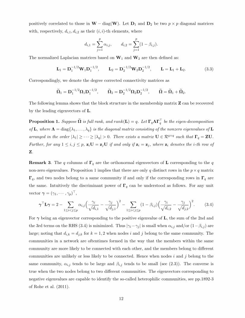
positively correlated to those in W − diag(W). Let D1 and D2 be two p × p diagonal matrices

with, respectively, di,1, di,2 as their (i, i)-th elements, where

di,1 =

p∑j=1

αi,j , di,2 =

p∑j=1

(1− βi,j).

The normalized Laplacian matrices based on W1 and W2 are then defined as:

L1 = D−1/21 W1D

−1/21 , L2 = D

−1/22 W2D

−1/22 , L = L1 + L2. (3.3)

Correspondingly, we denote the degree corrected connectivity matrices as

Ω1 = D−1/21 Ω1D

−1/21 , Ω2 = D

−1/22 Ω2D

−1/22 , Ω = Ω1 + Ω2.

The following lemma shows that the block structure in the membership matrix Z can be recovered

by the leading eigenvectors of L.

Proposition 1. Suppose Ω is full rank, and rank(L) = q. Let ΓqΛΓ>q be the eigen-decomposition

of L, where Λ = diagλ1, . . . , λq is the diagonal matrix consisting of the nonzero eigenvalues of L

arranged in the order |λ1| ≥ · · · ≥ |λq| > 0. There exists a matrix U ∈ Rq×q such that Γq = ZU.

Further, for any 1 ≤ i, j ≤ p, ziU = zjU if and only if zi = zj, where zi denotes the i-th row of

Z.

Remark 3. The q columns of Γq are the orthonormal eigenvectors of L corresponding to the q

non-zero eigenvalues. Proposition 1 implies that there are only q distinct rows in the p× q matrix

Γq, and two nodes belong to a same community if and only if the corresponding rows in Γq are

the same. Intuitively the discriminant power of Γq can be understood as follows. For any unit

vector γ = (γ1, · · · , γp)>,

γ>Lγ = 2−∑

1≤i<j≤pαi,j

( γi√di,1− γj√

dj,1

)2−

∑1≤i<j≤p

(1− βi,j)( γi√

di,2− γj√

dj,2

)2. (3.4)

For γ being an eigenvector corresponding to the positive eigenvalue of L, the sum of the 2nd and

the 3rd terms on the RHS (3.4) is minimized. Thus |γi−γj | is small when αi,j and/or (1−βi,j) are

large; noting that di,k = dj,k for k = 1, 2 when nodes i and j belong to the same community. The

communities in a network are oftentimes formed in the way that the members within the same

community are more likely to be connected with each other, and the members belong to different

communities are unlikely or less likely to be connected. Hence when nodes i and j belong to the

same community, αi,j tends to be large and βi,j tends to be small (see (2.3)). The converse is

true when the two nodes belong to two different communities. The eigenvectors corresponding to

negative eigenvalues are capable to identify the so-called heterophilic communities, see pp.1892-3

of Rohe et al. (2011).

12

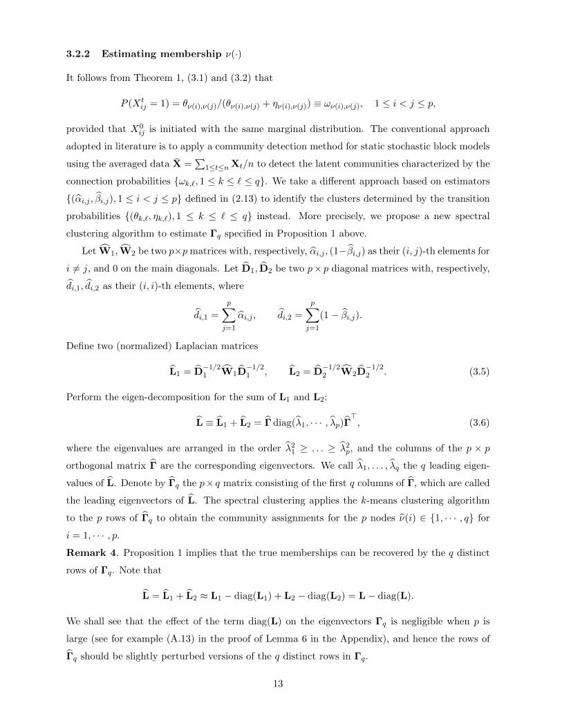
3.2.2 Estimating membership ν(·)

It follows from Theorem 1, (3.1) and (3.2) that

P (Xtij = 1) = θν(i),ν(j)/(θν(i),ν(j) + ην(i),ν(j)) ≡ ων(i),ν(j), 1 ≤ i < j ≤ p,

provided that X0ij is initiated with the same marginal distribution. The conventional approach

adopted in literature is to apply a community detection method for static stochastic block models

using the averaged data X =∑

1≤t≤n Xt/n to detect the latent communities characterized by the

connection probabilities ωk,`, 1 ≤ k ≤ ` ≤ q. We take a different approach based on estimators

(αi,j , βi,j), 1 ≤ i < j ≤ p defined in (2.13) to identify the clusters determined by the transition

probabilities (θk,`, ηk,`), 1 ≤ k ≤ ` ≤ q instead. More precisely, we propose a new spectral

clustering algorithm to estimate Γq specified in Proposition 1 above.

Let W1,W2 be two p×p matrices with, respectively, αi,j , (1−βi,j) as their (i, j)-th elements for

i 6= j, and 0 on the main diagonals. Let D1, D2 be two p× p diagonal matrices with, respectively,

di,1, di,2 as their (i, i)-th elements, where

di,1 =

p∑j=1

αi,j , di,2 =

p∑j=1

(1− βi,j).

Define two (normalized) Laplacian matrices

L1 = D−1/21 W1D

−1/21 , L2 = D

−1/22 W2D

−1/22 . (3.5)

Perform the eigen-decomposition for the sum of L1 and L2:

L ≡ L1 + L2 = Γ diag(λ1, · · · , λp)Γ>, (3.6)

where the eigenvalues are arranged in the order λ21 ≥ . . . ≥ λ2

p, and the columns of the p × p

orthogonal matrix Γ are the corresponding eigenvectors. We call λ1, . . . , λq the q leading eigen-

values of L. Denote by Γq the p× q matrix consisting of the first q columns of Γ, which are called

the leading eigenvectors of L. The spectral clustering applies the k-means clustering algorithm

to the p rows of Γq to obtain the community assignments for the p nodes ν(i) ∈ 1, · · · , q for

i = 1, · · · , p.

Remark 4. Proposition 1 implies that the true memberships can be recovered by the q distinct

rows of Γq. Note that

L = L1 + L2 ≈ L1 − diag(L1) + L2 − diag(L2) = L− diag(L).

We shall see that the effect of the term diag(L) on the eigenvectors Γq is negligible when p is

large (see for example (A.13) in the proof of Lemma 6 in the Appendix), and hence the rows of

Γq should be slightly perturbed versions of the q distinct rows in Γq.

13

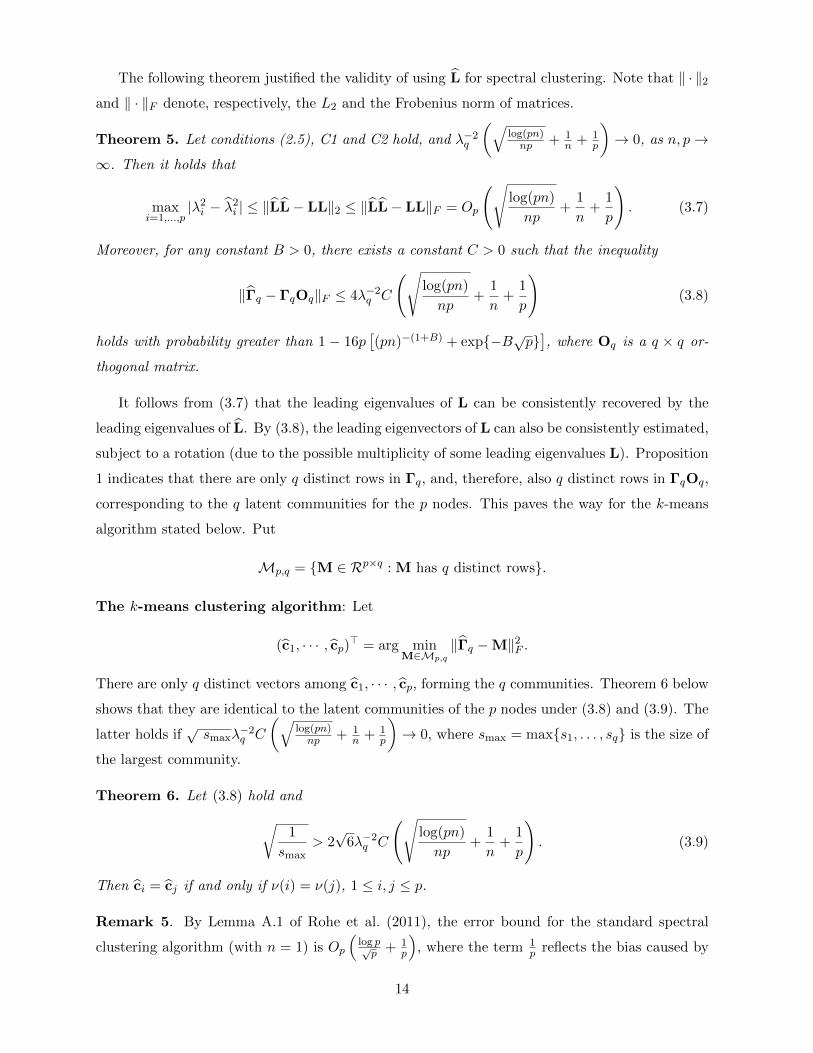
The following theorem justified the validity of using L for spectral clustering. Note that ‖ · ‖2and ‖ · ‖F denote, respectively, the L2 and the Frobenius norm of matrices.

Theorem 5. Let conditions (2.5), C1 and C2 hold, and λ−2q

(√log(pn)np + 1

n + 1p

)→ 0, as n, p→

∞. Then it holds that

maxi=1,...,p

|λ2i − λ2

i | ≤ ‖LL− LL‖2 ≤ ‖LL− LL‖F = Op

(√log(pn)

np+

1

n+

1

p

). (3.7)

Moreover, for any constant B > 0, there exists a constant C > 0 such that the inequality

‖Γq − ΓqOq‖F ≤ 4λ−2q C

(√log(pn)

np+

1

n+

1

p

)(3.8)

holds with probability greater than 1 − 16p[(pn)−(1+B) + exp−B√p

], where Oq is a q × q or-

thogonal matrix.

It follows from (3.7) that the leading eigenvalues of L can be consistently recovered by the

leading eigenvalues of L. By (3.8), the leading eigenvectors of L can also be consistently estimated,

subject to a rotation (due to the possible multiplicity of some leading eigenvalues L). Proposition

1 indicates that there are only q distinct rows in Γq, and, therefore, also q distinct rows in ΓqOq,

corresponding to the q latent communities for the p nodes. This paves the way for the k-means

algorithm stated below. Put

Mp,q = M ∈ Rp×q : M has q distinct rows.

The k-means clustering algorithm: Let

(c1, · · · , cp)> = arg minM∈Mp,q

‖Γq −M‖2F .

There are only q distinct vectors among c1, · · · , cp, forming the q communities. Theorem 6 below

shows that they are identical to the latent communities of the p nodes under (3.8) and (3.9). The

latter holds if√smaxλ

−2q C

(√log(pn)np + 1

n + 1p

)→ 0, where smax = maxs1, . . . , sq is the size of

the largest community.

Theorem 6. Let (3.8) hold and√1

smax> 2√

6λ−2q C

(√log(pn)

np+

1

n+

1

p

). (3.9)

Then ci = cj if and only if ν(i) = ν(j), 1 ≤ i, j ≤ p.

Remark 5. By Lemma A.1 of Rohe et al. (2011), the error bound for the standard spectral

clustering algorithm (with n = 1) is Op

(log p√p + 1

p

), where the term 1

p reflects the bias caused by

14

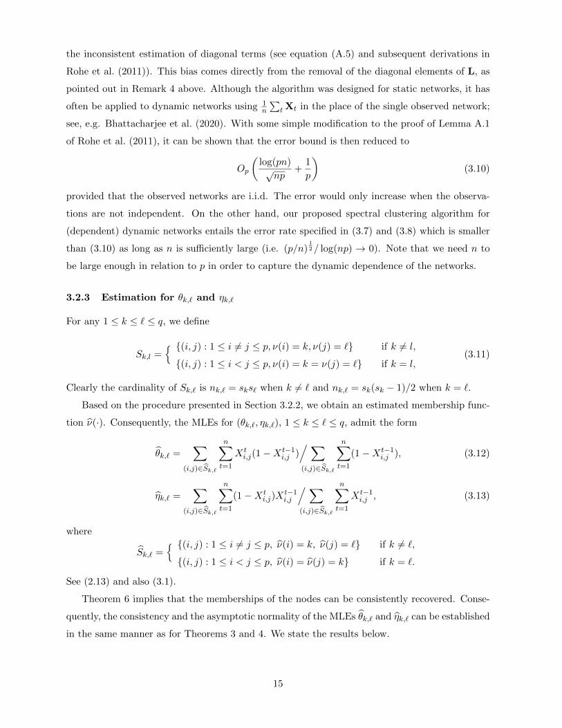
the inconsistent estimation of diagonal terms (see equation (A.5) and subsequent derivations in

Rohe et al. (2011)). This bias comes directly from the removal of the diagonal elements of L, as

pointed out in Remark 4 above. Although the algorithm was designed for static networks, it has

often be applied to dynamic networks using 1n

∑t Xt in the place of the single observed network;

see, e.g. Bhattacharjee et al. (2020). With some simple modification to the proof of Lemma A.1

of Rohe et al. (2011), it can be shown that the error bound is then reduced to

Op

(log(pn)√np

+1

p

)(3.10)

provided that the observed networks are i.i.d. The error would only increase when the observa-

tions are not independent. On the other hand, our proposed spectral clustering algorithm for

(dependent) dynamic networks entails the error rate specified in (3.7) and (3.8) which is smaller

than (3.10) as long as n is sufficiently large (i.e. (p/n)12 / log(np) → 0). Note that we need n to

be large enough in relation to p in order to capture the dynamic dependence of the networks.

3.2.3 Estimation for θk,` and ηk,`

For any 1 ≤ k ≤ ` ≤ q, we define

Sk,l = (i, j) : 1 ≤ i 6= j ≤ p, ν(i) = k, ν(j) = ` if k 6= l,

(i, j) : 1 ≤ i < j ≤ p, ν(i) = k = ν(j) = ` if k = l,(3.11)

Clearly the cardinality of Sk,` is nk,` = sks` when k 6= ` and nk,` = sk(sk − 1)/2 when k = `.

Based on the procedure presented in Section 3.2.2, we obtain an estimated membership func-

tion ν(·). Consequently, the MLEs for (θk,`, ηk,`), 1 ≤ k ≤ ` ≤ q, admit the form

θk,` =∑

(i,j)∈Sk,`

n∑t=1

Xti,j(1−Xt−1

i,j )/∑(i,j)∈Sk,`

n∑t=1

(1−Xt−1i,j ), (3.12)

ηk,` =∑

(i,j)∈Sk,`

n∑t=1

(1−Xti,j)X

t−1i,j

/∑(i,j)∈Sk,`

n∑t=1

Xt−1i,j , (3.13)

where

Sk,` = (i, j) : 1 ≤ i 6= j ≤ p, ν(i) = k, ν(j) = ` if k 6= `,

(i, j) : 1 ≤ i < j ≤ p, ν(i) = ν(j) = k if k = `.

See (2.13) and also (3.1).

Theorem 6 implies that the memberships of the nodes can be consistently recovered. Conse-

quently, the consistency and the asymptotic normality of the MLEs θk,` and ηk,` can be established

in the same manner as for Theorems 3 and 4. We state the results below.

15

Let K1 = (i1, j1), . . . , (im1 , jm1) and K2 = (k1, `1), . . . , (km2 , `m2) be two arbitrary subsets

of (k, `) : 1 ≤ k ≤ ` ≤ q with m1,m2 ≥ 1 fixed. Let

ΨK1,K2 = (θi1,j1 , . . . , θim1 ,jm1, ηk1,`1 , . . . , ηkm2 ,`m2

)′,

and let ΨK1,K2 denote its MLE. Put NK1,K2 = diag(ni1,j1 , . . . , nim1 ,jm1, nk1,`1 , . . . , nkm2 ,`m2

) where

nk,` is the cardinality of Sk,` defined as in (3.11).

Theorem 7. Let conditions (2.5), C1 and C2 hold, and√smaxλ

−2q C

(√log(pn)np + 1

n + 1p

)→ 0.

Then it holds that

max1≤k,`≤q

|θk,` − θk,`| = Op

(√log q

ns2min

)and max

1≤k,`≤q|ηk,` − ηk,`| = Op

(√log q

ns2min

),

where smin = mins1, . . . , sq.

Theorem 8. Let the condition of Theorem 7 holds. Then

√nN

12K1,K2

(ΨK1,K2 −ΨK1,K2)→ N(0, ΣK1,K2),

where ΣK1,K2 = diag(σ11, . . . , σm1+m2,m1+m2) with

σrr =θir,jr(1− θir,jr)(θir,jr + ηir,jr)

ηir,jr, 1 ≤ r ≤ m1,

σrr =ηkr,`r(1− ηkr,`r)(θkr,`r + ηkr,`r)

θkr,`r, m1 + 1 ≤ r ≤ m1 +m2.

Finally to prepare for the inference in Section 3.3 below, we introduce some notation. First we

denote ν by ν1,n, to reflect the fact that the community clustering was carried out using the data

X1, · · · ,Xn (conditionally on X0). See Section 3.2.2 above. Further we denote the maximum log

likelihood by

l(1, n; ν1,n) = l(θk,`, ηk,`; ν1,n) (3.14)

to highlight the fact that both the node clustering and the estimation for transition probabilities

are based on the data X1, · · · ,Xn.

3.3 Inference with a change-point

Now we assume that there is a change-point τ0 at which both the membership of nodes and the

transition probabilities θk,`, ηk,` change. It is necessary to assume n0 ≤ τ0 ≤ n− n0, where n0

is an integer and n0/n ≡ c0 > 0 is a small constant, as we need enough information before and

after the change in order to detect τ0. We assume that within the time period [0, τ0], the network

16

follows a stationary model (3.2) with parameters (θ1,k,`, η1,k,`) : 1 ≤ k, l ≤ q and a membership

map ν1,τ0(·). Within the time period [τ0 + 1, n] the network follows a stationary model (3.2) with

parameters (θ2,k,`, η2,k,`) : 1 ≤ k, l ≤ q and a membership map ντ0+1,n(·). Though we assume

that the number of communities is unchanged after the change point, our results can be easily

extended to the case that the number of communities also changes.

We estimate the change point τ0 by the maximum likelihood method:

τ = arg maxn0≤τ≤n−n0

l(1, τ ; ν1,τ ) + l(τ + 1, n; ντ+1,n), (3.15)

where l(·) is given in (3.14).

To measure the difference between the two sets of transition probabilities before and after the

change, we put

∆2F =

1

p2

(‖W1,1 −W2,1‖2F + ‖W1,2 −W2,2‖2F

),

where the four p× p matrices are defined as

W1,1 = (θ1,ν1,τ0 (i),ν1,τ0 (j)), W1,2 = (1− η1,ν1,τ0 (i),ν1,τ0 (j)),

W2,1 = (θ2,ντ0+1,n(i),ντ0 (j)+1,n), W2,2 = (1− η1,ντ0+1,n(i),ντ0+1,n(j)).

Note that ∆F can be viewed as the signal strength for detecting the change-point τ0. Let

smax, smin denote, respectively, the largest, the smallest community size among all the communi-

ties before and after the change. Similar to (3.3), we denote the normalized Laplacian matrices

corresponding to on Wi,j as Li,j for i, j = 1, 2. Let |λi,1| ≥ |λi,2| ≥ . . . ≥ |λi,q| the absolute

nonzero eigenvalues of Li,1 + Li,2 for i = 1, 2, and we denote λmin = min|λ1,q|, |λ2,q|. Now some

regularity conditions are in order.

C3. For some constant l > 0, θi,k,`, ηi,k,` > l, and θi,k,` + ηi,k,` ≤ 1 for all i = 1, 2 and 1 ≤ k ≤

` ≤ q.

C4. log(np)/√p→ 0, and

√smaxλ

−2min

(√log(pn)/np+ 1

n + 1p +

log(np)/n+√

log(np)/(np2)

∆2F

)→ 0.

C5.∆2F

log(np)/n+√

log(np)/(np2)→∞.

Condition C3 is similar to C1. The condition log(np)/√p→ 0 in C4 controls the misclassification

rate of the k-means algorithm. Recall that there is a bias term O(p−1) in spectral clustering

caused by the removal of the diagonal of the Laplacian matrix (see Remark 4 above). Intuitively,

as p increases, the effect of this bias term on the misclassification rate of the k-means algorithm

becomes negligible. On the other hand, note that the length of the time interval for searching

for the change point in (3.15) is of order O(n), the log(n) term here in some sense reflects the

17

effect of the difficulty in detecting the true change point when the searching interval is extended

as n increases. The second condition in C4 is similar to (3.9), which ensures that the true

communities can be recovered. Condition C5 requires that the average signal strength ∆2F =

p−2[‖W1,1 −W2,1‖2F + ‖W1,2 −W2,2‖2F

]is of higher order than log(np)

n +√

log(np)np2

for change

point detection.

Theorem 9. Let conditions C2-C5 hold. Then the following assertions hold.

(i) When ν1,τ0 ≡ ντ0+1,n,

|τ0 − τ |n

= Op

log(np)n +

√log(np)np2

∆2F

×min

1,

min

1, (n−1p2 log(np))14

∆F smin

.

(ii) When ν1,τ0 6= ντ0+1,n,

|τ0 − τ |n

= Op

( log(np)n +

√log(np)np2

∆2F

×min

1,min

1, (n−1p2 log(np))

14

∆F smin

+1

∆2F

.

Notice that for τ < τ0, the observations in the time interval [τ + 1, n] are a mixture of the two

different network processes if ν1,τ0 6= ντ0+1,n. In the worst case scenario then, all q communities

can be changed after the change point τ0. This causes the extra estimation error term 1∆2F

in

Theorem 9(ii).

4 Simulations

4.1 Parameter estimation

We generate data according to model (2.1) in which the parameters αij and βij are drawn inde-

pendently from U [0.1, 0.5], 1 ≤ i, j ≤ p. The initial value X0 was simulated according to (2.6)

with πij = 0.5. We calculate the estimates according to (2.13). For each setting (with different p

and n), we replicate the experiment 500 times. Furthermore we also calculate the 95% confidence

intervals for αij and βij based on the asymptotically normal distributions specified in Theorem

4, and report the relative frequencies of the intervals covering the true values of the parameters.

The results are summarized in Table 1.

The MSE decreases as n increases, showing steadily improvement in performance. The cover-

age rates of the asymptotic confidence intervals are very close to the nominal level when n ≥ 50.

The results hardly change between p = 100 and 200.

18

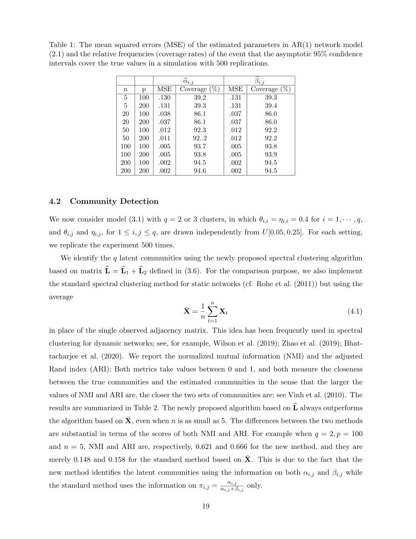
Table 1: The mean squared errors (MSE) of the estimated parameters in AR(1) network model(2.1) and the relative frequencies (coverage rates) of the event that the asymptotic 95% confidenceintervals cover the true values in a simulation with 500 replications.

αi,j βi,jn p MSE Coverage (%) MSE Coverage (%)5 100 .130 39.2 .131 39.35 200 .131 39.3 .131 39.420 100 .038 86.1 .037 86.020 200 .037 86.1 .037 86.050 100 .012 92.3 .012 92.250 200 .011 92..2 .012 92.2100 100 .005 93.7 .005 93.8100 200 .005 93.8 .005 93.9200 100 .002 94.5 .002 94.5200 200 .002 94.6 .002 94.5

4.2 Community Detection

We now consider model (3.1) with q = 2 or 3 clusters, in which θi,i = ηi,i = 0.4 for i = 1, · · · , q,

and θi,j and ηi,j , for 1 ≤ i, j ≤ q, are drawn independently from U [0.05, 0.25]. For each setting,

we replicate the experiment 500 times.

We identify the q latent communities using the newly proposed spectral clustering algorithm

based on matrix L = L1 + L2 defined in (3.6). For the comparison purpose, we also implement

the standard spectral clustering method for static networks (cf. Rohe et al. (2011)) but using the

average

X =1

n

n∑t=1

Xt (4.1)

in place of the single observed adjacency matrix. This idea has been frequently used in spectral

clustering for dynamic networks; see, for example, Wilson et al. (2019); Zhao et al. (2019); Bhat-

tacharjee et al. (2020). We report the normalized mutual information (NMI) and the adjusted

Rand index (ARI): Both metrics take values between 0 and 1, and both measure the closeness

between the true communities and the estimated communities in the sense that the larger the

values of NMI and ARI are, the closer the two sets of communities are; see Vinh et al. (2010). The

results are summarized in Table 2. The newly proposed algorithm based on L always outperforms

the algorithm based on X, even when n is as small as 5. The differences between the two methods

are substantial in terms of the scores of both NMI and ARI. For example when q = 2, p = 100

and n = 5, NMI and ARI are, respectively, 0.621 and 0.666 for the new method, and they are

merely 0.148 and 0.158 for the standard method based on X. This is due to the fact that the

new method identifies the latent communities using the information on both αi,j and βi,j while

the standard method uses the information on πi,j =αi,j

αi,j+βi,jonly.

19

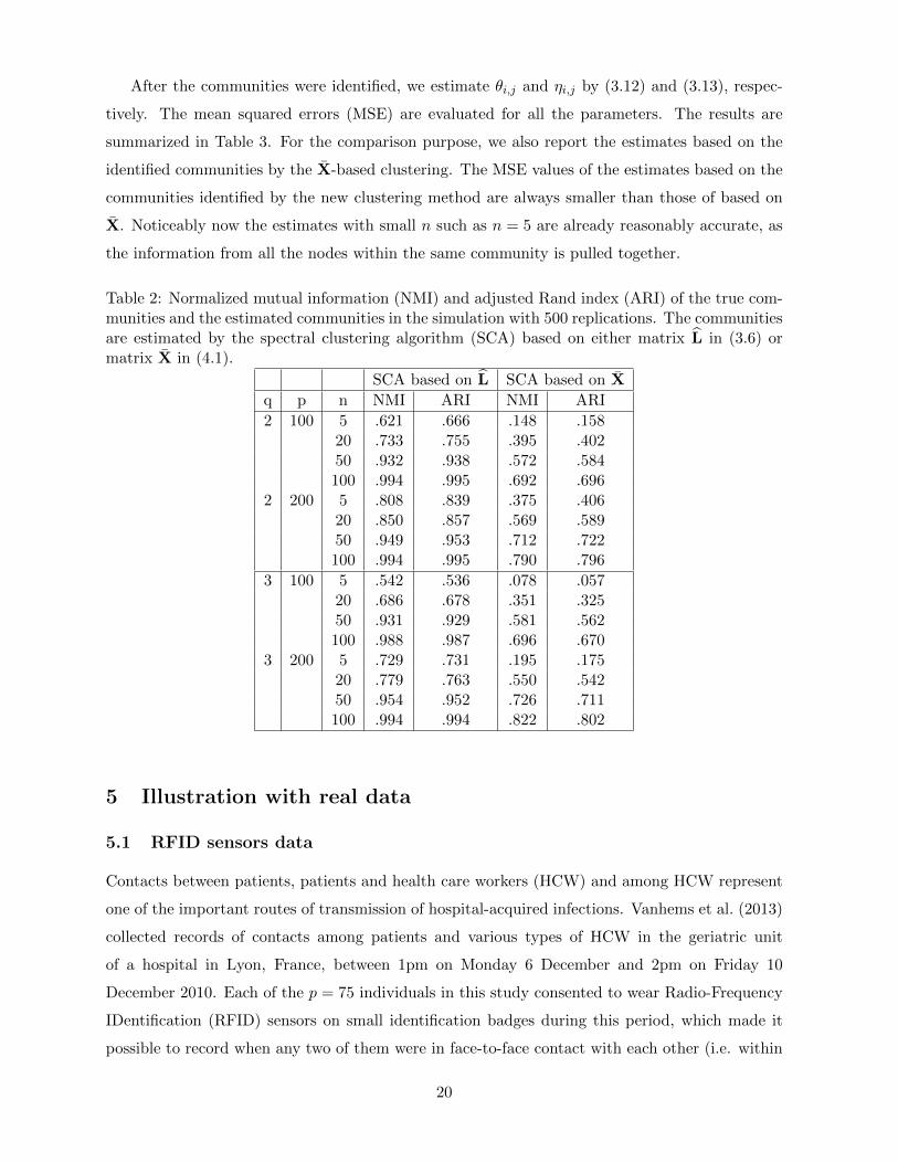
After the communities were identified, we estimate θi,j and ηi,j by (3.12) and (3.13), respec-

tively. The mean squared errors (MSE) are evaluated for all the parameters. The results are

summarized in Table 3. For the comparison purpose, we also report the estimates based on the

identified communities by the X-based clustering. The MSE values of the estimates based on the

communities identified by the new clustering method are always smaller than those of based on

X. Noticeably now the estimates with small n such as n = 5 are already reasonably accurate, as

the information from all the nodes within the same community is pulled together.

Table 2: Normalized mutual information (NMI) and adjusted Rand index (ARI) of the true com-munities and the estimated communities in the simulation with 500 replications. The communitiesare estimated by the spectral clustering algorithm (SCA) based on either matrix L in (3.6) ormatrix X in (4.1).

SCA based on L SCA based on X

q p n NMI ARI NMI ARI

2 100 5 .621 .666 .148 .15820 .733 .755 .395 .40250 .932 .938 .572 .584100 .994 .995 .692 .696

2 200 5 .808 .839 .375 .40620 .850 .857 .569 .58950 .949 .953 .712 .722100 .994 .995 .790 .796

3 100 5 .542 .536 .078 .05720 .686 .678 .351 .32550 .931 .929 .581 .562100 .988 .987 .696 .670

3 200 5 .729 .731 .195 .17520 .779 .763 .550 .54250 .954 .952 .726 .711100 .994 .994 .822 .802

5 Illustration with real data

5.1 RFID sensors data

Contacts between patients, patients and health care workers (HCW) and among HCW represent

one of the important routes of transmission of hospital-acquired infections. Vanhems et al. (2013)

collected records of contacts among patients and various types of HCW in the geriatric unit

of a hospital in Lyon, France, between 1pm on Monday 6 December and 2pm on Friday 10

December 2010. Each of the p = 75 individuals in this study consented to wear Radio-Frequency

IDentification (RFID) sensors on small identification badges during this period, which made it

possible to record when any two of them were in face-to-face contact with each other (i.e. within

20

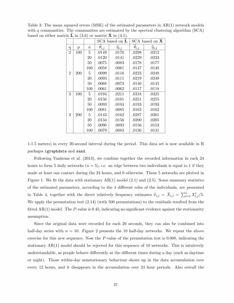
Table 3: The mean squared errors (MSE) of the estimated parameters in AR(1) network modelswith q communities. The communities are estimated by the spectral clustering algorithm (SCA)based on either matrix L in (3.6) or matrix X in (4.1).

SCA based on L SCA based on X

q p n θi,j ηi,j θi,j ηi,j2 100 5 .0149 .0170 .0298 .0312

20 .0120 .0141 .0229 .023350 .0075 .0083 .0178 .0177100 .0058 .0061 .0147 .0148

2 200 5 .0099 .0116 .0223 .024820 .0093 .0111 .0219 .024850 .0068 .0073 .0140 .0145100 .0061 .0062 .0117 .0118

3 100 5 .0194 .0211 .0318 .032520 .0156 .0181 .0251 .025550 .0093 .0104 .0193 .0193100 .0081 .0085 .0163 .0162

3 200 5 .0143 .0162 .0287 .030120 .0134 .0156 .0200 .020550 .0090 .0093 .0156 .0153100 .0079 .0083 .0130 .0131

1-1.5 meters) in every 20-second interval during the period. This data set is now available in R

packages igraphdata and sand.

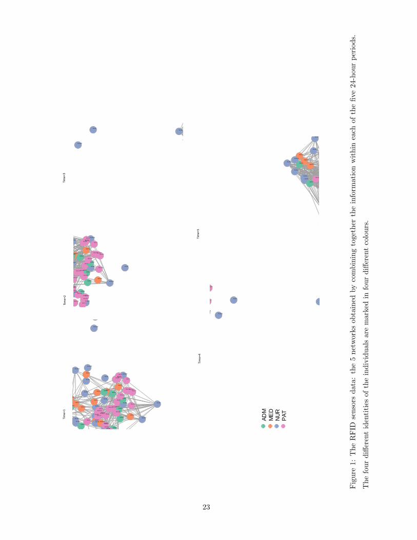
Following Vanhems et al. (2013), we combine together the recorded information in each 24

hours to form 5 daily networks (n = 5), i.e. an edge between two individuals is equal to 1 if they

made at least one contact during the 24 hours, and 0 otherwise. Those 5 networks are plotted in

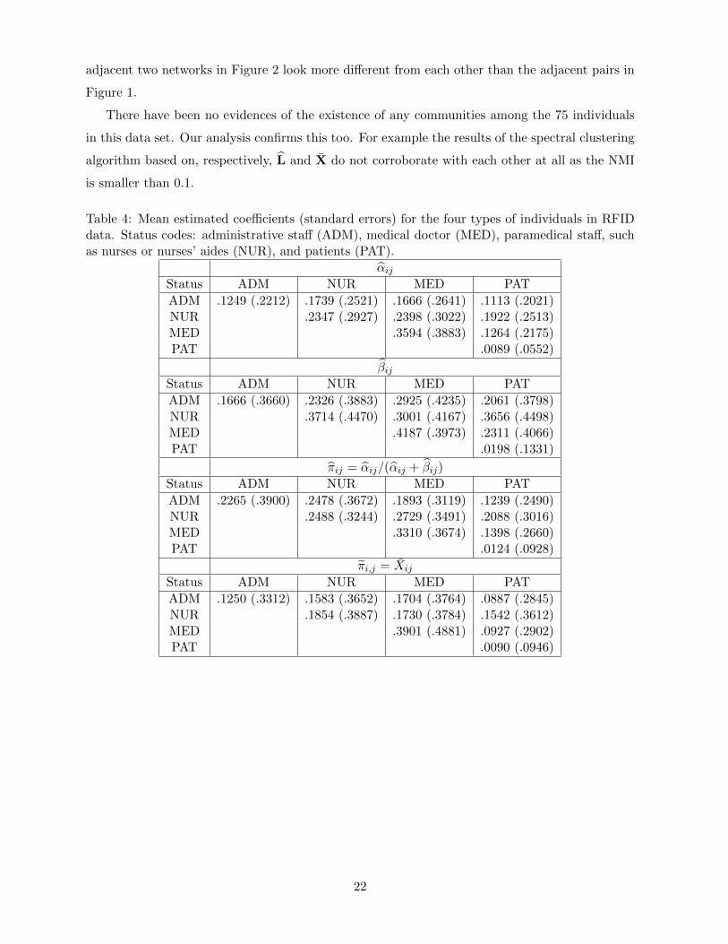
Figure 1. We fit the data with stationary AR(1) model (2.1) and (2.5). Some summary statistics

of the estimated parameters, according to the 4 different roles of the individuals, are presented

in Table 4, together with the direct relatively frequency estimates πi,j = Xi,j =∑5

t=1Xti,j/5.

We apply the permutation test (2.14) (with 500 permutations) to the residuals resulted from the

fitted AR(1) model. The P -value is 0.45, indicating no significant evidence against the stationarity

assumption.

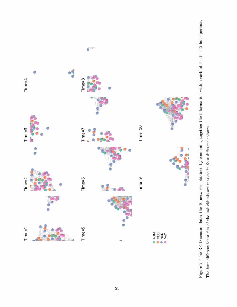
Since the original data were recorded for each 20 seconds, they can also be combined into

half-day series with n = 10. Figure 2 presents the 10 half-day networks. We repeat the above

exercise for this new sequence. Now the P -value of the permutation test is 0.008, indicating the

stationary AR(1) model should be rejected for this sequence of 10 networks. This is intuitively

understandable, as people behave differently at the different times during a day (such as daytime

or night). Those within-day nonstationary behaviour shows up in the data accumulation over

every 12 hours, and it disappears in the accumulation over 24 hour periods. Also overall the

21

adjacent two networks in Figure 2 look more different from each other than the adjacent pairs in

Figure 1.

There have been no evidences of the existence of any communities among the 75 individuals

in this data set. Our analysis confirms this too. For example the results of the spectral clustering

algorithm based on, respectively, L and X do not corroborate with each other at all as the NMI

is smaller than 0.1.

Table 4: Mean estimated coefficients (standard errors) for the four types of individuals in RFIDdata. Status codes: administrative staff (ADM), medical doctor (MED), paramedical staff, suchas nurses or nurses’ aides (NUR), and patients (PAT).

αijStatus ADM NUR MED PAT

ADM .1249 (.2212) .1739 (.2521) .1666 (.2641) .1113 (.2021)NUR .2347 (.2927) .2398 (.3022) .1922 (.2513)MED .3594 (.3883) .1264 (.2175)PAT .0089 (.0552)

βijStatus ADM NUR MED PAT

ADM .1666 (.3660) .2326 (.3883) .2925 (.4235) .2061 (.3798)NUR .3714 (.4470) .3001 (.4167) .3656 (.4498)MED .4187 (.3973) .2311 (.4066)PAT .0198 (.1331)

πij = αij/(αij + βij)

Status ADM NUR MED PAT

ADM .2265 (.3900) .2478 (.3672) .1893 (.3119) .1239 (.2490)NUR .2488 (.3244) .2729 (.3491) .2088 (.3016)MED .3310 (.3674) .1398 (.2660)PAT .0124 (.0928)

πi,j = Xij

Status ADM NUR MED PAT

ADM .1250 (.3312) .1583 (.3652) .1704 (.3764) .0887 (.2845)NUR .1854 (.3887) .1730 (.3784) .1542 (.3612)MED .3901 (.4881) .0927 (.2902)PAT .0090 (.0946)

22

Time=1

Time=2

Time=3

Time=4

Time=5

AD

M1

NU

R1

NU

R2

NU

R3

NU

R4

NU

R5

NU

R6

NU

R7

ME

D1

NU

R8

ME

D2

ME

D3

NU

R9

ME

D4

ME

D5

ME

D6

NU

R10

ME

D7

AD

M2N

UR

11

NU

R12

ME

D8

NU

R13

NU

R14

NU

R15

NU

R16

NU

R17

AD

M3

NU

R18

ME

D9

AD

M4

NU

R19

NU

R20

NU

R21

ME

D10

NU

R22

NU

R23

PA

T1

PA

T2

PA

T3

PA

T4

PA

T5

PA

T6

PA

T7

PA

T8

PA

T9

PA

T10

PA

T11

PA

T12

PA

T13

PA

T14

PA

T15

PA

T16

PA

T17

PA

T18

PA

T19

NU

R24

AD

M5 A

DM

6

PA

T20

NU

R25

NU

R26

NU

R27

AD

M7

ME

D11

PA

T21

PA

T22

PA

T23

PA

T24

PA

T25

AD

M8

PA

T26

PA

T27

PA

T28

PA

T29

AD

M

ME

D

NU

R

PA

T

AD

M

ME

D

NU

R

PA

T

Fig

ure

1:T

he

RF

IDse

nso

rsd

ata

:th

e5

net

wor

ks

obta

ined

by

com

bin

ing

toge

ther

the

info

rmat

ion

wit

hin

each

ofth

efi

ve24

-hou

rp

erio

ds.

Th

efo

ur

diff

eren

tid

enti

ties

ofth

ein

div

idu

als

are

mar

ked

info

ur

diff

eren

tco

lou

rs.

23

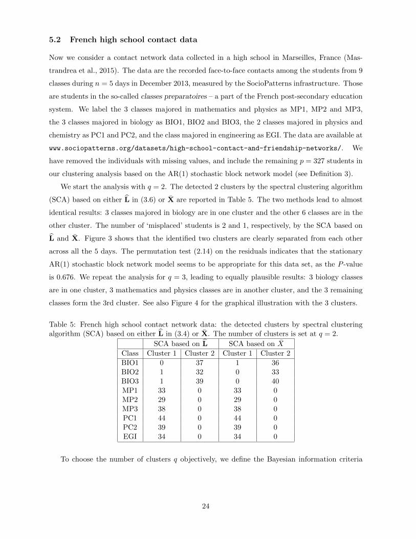
5.2 French high school contact data

Now we consider a contact network data collected in a high school in Marseilles, France (Mas-

trandrea et al., 2015). The data are the recorded face-to-face contacts among the students from 9

classes during n = 5 days in December 2013, measured by the SocioPatterns infrastructure. Those

are students in the so-called classes preparatoires – a part of the French post-secondary education

system. We label the 3 classes majored in mathematics and physics as MP1, MP2 and MP3,

the 3 classes majored in biology as BIO1, BIO2 and BIO3, the 2 classes majored in physics and

chemistry as PC1 and PC2, and the class majored in engineering as EGI. The data are available at

www.sociopatterns.org/datasets/high-school-contact-and-friendship-networks/. We

have removed the individuals with missing values, and include the remaining p = 327 students in

our clustering analysis based on the AR(1) stochastic block network model (see Definition 3).

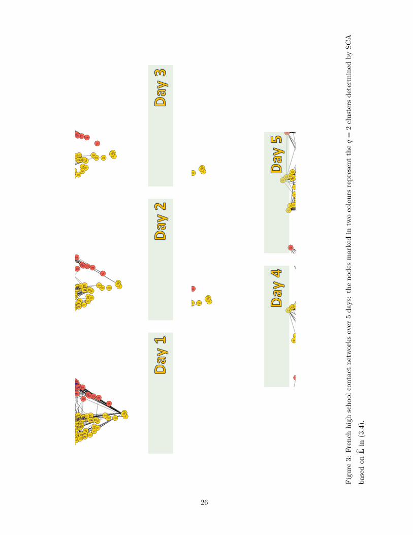
We start the analysis with q = 2. The detected 2 clusters by the spectral clustering algorithm

(SCA) based on either L in (3.6) or X are reported in Table 5. The two methods lead to almost

identical results: 3 classes majored in biology are in one cluster and the other 6 classes are in the

other cluster. The number of ‘misplaced’ students is 2 and 1, respectively, by the SCA based on

L and X. Figure 3 shows that the identified two clusters are clearly separated from each other

across all the 5 days. The permutation test (2.14) on the residuals indicates that the stationary

AR(1) stochastic block network model seems to be appropriate for this data set, as the P -value

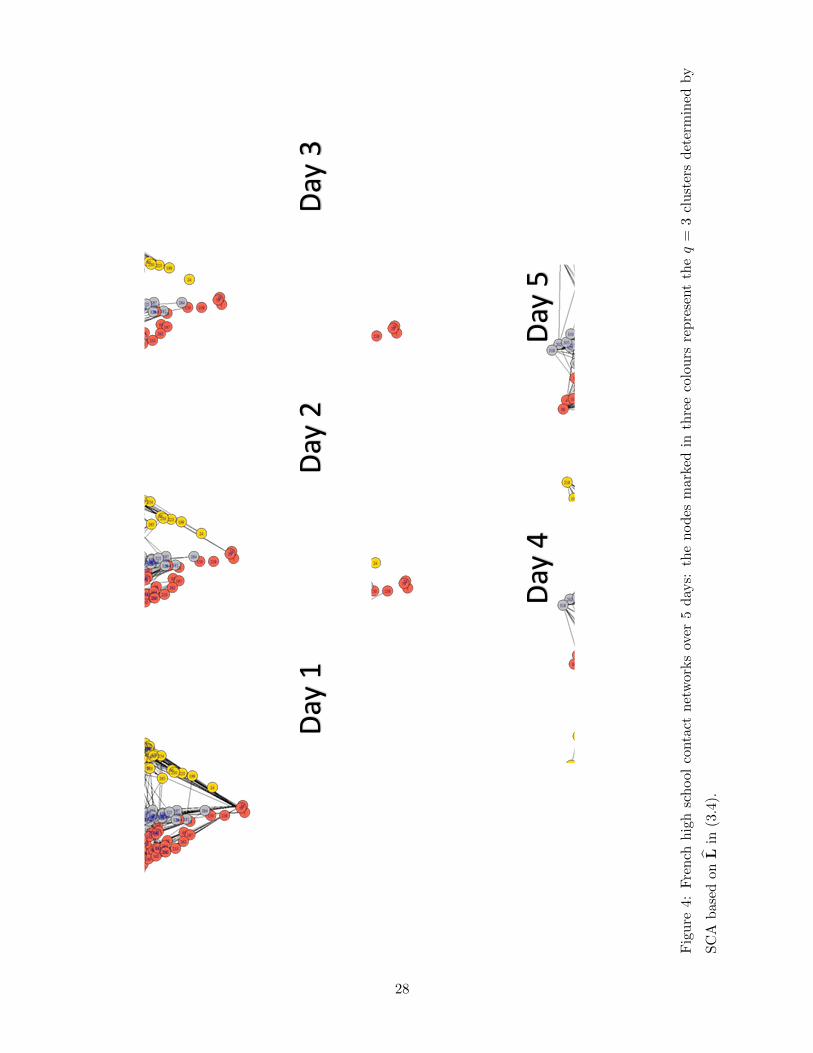
is 0.676. We repeat the analysis for q = 3, leading to equally plausible results: 3 biology classes

are in one cluster, 3 mathematics and physics classes are in another cluster, and the 3 remaining

classes form the 3rd cluster. See also Figure 4 for the graphical illustration with the 3 clusters.

Table 5: French high school contact network data: the detected clusters by spectral clusteringalgorithm (SCA) based on either L in (3.4) or X. The number of clusters is set at q = 2.

SCA based on L SCA based on X

Class Cluster 1 Cluster 2 Cluster 1 Cluster 2

BIO1 0 37 1 36BIO2 1 32 0 33BIO3 1 39 0 40MP1 33 0 33 0MP2 29 0 29 0MP3 38 0 38 0PC1 44 0 44 0PC2 39 0 39 0EGI 34 0 34 0

To choose the number of clusters q objectively, we define the Bayesian information criteria

24

Time=1

Time=2

Time=3

Time=4

Time=5

Time=6

Time=7

Time=8

Time=9

Time=10

AD

M1

NU

R1

NU

R2

NU

R3

NU

R4

NU

R5

NU

R6

NU

R7

ME

D1

NU

R8

ME

D2

ME

D3

NU

R9

ME

D4

ME

D5

ME

D6

NU

R10

ME

D7

AD

M2N

UR

11

NU

R12

ME

D8

NU

R13

NU

R14

NU

R15

NU

R16

NU

R17

AD

M3

NU

R18

ME

D9

AD

M4

NU

R19

NU

R20

NU

R21

ME

D10

NU

R22

NU

R23

PA

T1

PA

T2

PA

T3

PA

T4

PA

T5

PA

T6

PA

T7

PA

T8

PA

T9

PA

T10

PA

T11

PA

T12

PA

T13

PA

T14

PA

T15

PA

T16

PA

T17

PA

T18

PA

T19

NU

R24

AD

M5 A

DM

6

PA

T20

NU

R25

NU

R26

NU

R27

AD

M7

ME

D11

PA

T21

PA

T22

PA

T23

PA

T24

PA

T25

AD

M8

PA

T26

PA

T27

PA

T28

PA

T29

AD

M

ME

D

NU

R

PA

T

AD

M

ME

D

NU

R

PA

T

Fig

ure

2:

Th

eR

FID

sen

sors

data

:th

e10

net

wor

ks

obta

ined

by

com

bin

ing

toge

ther

the

info

rmat

ion

wit

hin

each

ofth

ete

n12

-hou

rp

erio

ds.

Th

efo

ur

diff

eren

tid

enti

ties

ofth

ein

div

idu

als

are

mar

ked

info

ur

diff

eren

tco

lou

rs.

25

Fig

ure

3:F

ren

chh

igh

sch

ool

conta

ctn

etw

ork

sov

er5

day

s:th

en

od

esm

arke

din

two

colo

urs

rep

rese

nt

theq

=2

clu

ster

sd

eter

min

edby

SC

A

base

don

Lin

(3.4

).

26

(BIC) as follows:

BIC(q) = −2 max log(likelihood) + logn(p/q)2q(q + 1).

For each fixed q, we effectively build q(q + 1)/2 models independently and each model has 2

parameters θk,` and ηk,`, 1 ≤ k ≤ ` ≤ q. The number of the available observations for each model

is approximately n(p/q)2, assuming that the numbers of nodes in all the q clusters are about the

same, which is then p/q. Thus the penalty term in the BIC above is∑

1≤k≤`≤q 2 logn(p/q)2 =

logn(p/q)2q(q + 1).

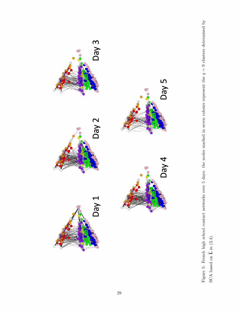
Table 6 lists the values of BIC(q) for different q. The minimum is obtained at q = 9, exactly

the number of original classes in the school. Performing the SCA based on L with q = 9, we

obtain almost perfect classification: all the 9 original classes are identified as the 9 clusters with

only in total 4 students being placed outside their own classes. Figure 5 plots the networks

with the identified 9 clusters in 9 different colours. The estimated θi,j and ηi,j , together with

their standard errors calculated based on the asymptotic normality presented in Theorem 8, are

reported in Table 7. As θi,j for i 6= j are very small (i.e. ≤ 0.027), the students from different

classes who have not contacted with each other are unlikely to contact next day. See (3.1) and

(2.3). On the other hand, as ηi,j for i 6= j are large (i.e. ≥ 0.761), the students from different

classes who have contacted with each other are likely to lose the contacts next day. Note that θi,i

are greater than θi,j for i 6= j substantially, and ηi,i are smaller than ηi,j for i 6= j substantially.

This implies that the students in the same class are more likely to contact with each other than

those across the different classes.

Table 6: Fitting AR(1) stochastic block models to the French high school data: BIC values fordifferent cluster numbers q.

q 2 3 5 7 8 9 10 11

BIC(q) 43624 40586 37726 36112 35224 34943 35002 35120

5.3 Global trade data

Our last example concerns the annual international trades among p = 197 countries between 1950

and 2014 (i.e. n = 65). We define an edge between two countries to be 1 as long as there exist

trades between the two countries in that year (regardless the direction), and 0 otherwise. We

take this simplistic approach to illustrate our AR(1) stochastic block model with a change-point.

The data used are a subset of the openly available trade data for 205 countries in 1870 – 2014

(Barbieri et al., 2009; Barbieri and Keshk, 2016). We leave out several countries, e.g. Russian

and Yugoslavia, which did not exist for the whole period concerned.

27

Day

1D

ay 2

Day

3

Day

4D

ay 5

Fig

ure

4:F

ren

chh

igh

sch

ool

conta

ctn

etw

orks

over

5d

ays:

the

nod

esm

arke

din

thre

eco

lou

rsre

pre

sent

theq

=3

clu

ster

sd

eter

min

edby

SC

Ab

ased

on

Lin

(3.4

).

28

Day

1D

ay 2

Day

3

Day

4D

ay 5

Fig

ure

5:

Fre

nch

hig

hsc

hool

conta

ctn

etw

orks

over

5d

ays:

the

nod

esm

arke

din

seve

nco

lou

rsre

pre

sent

theq

=9

clu

ster

sd

eter

min

edby

SC

Ab

ased

on

Lin

(3.4

).

29

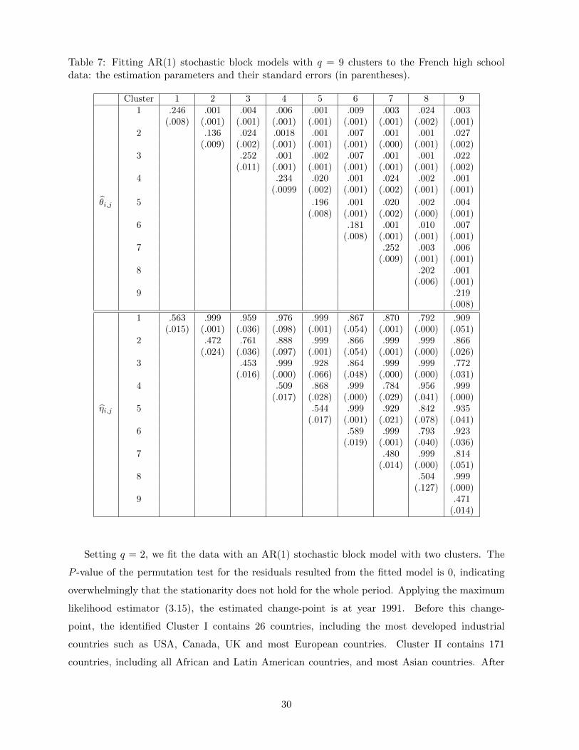
Table 7: Fitting AR(1) stochastic block models with q = 9 clusters to the French high schooldata: the estimation parameters and their standard errors (in parentheses).

Cluster 1 2 3 4 5 6 7 8 91 .246 .001 .004 .006 .001 .009 .003 .024 .003

(.008) (.001) (.001) (.001) (.001) (.001) (.001) (.002) (.001)2 .136 .024 .0018 .001 .007 .001 .001 .027

(.009) (.002) (.001) (.001) (.001) (.000) (.001) (.002)3 .252 .001 .002 .007 .001 .001 .022

(.011) (.001) (.001) (.001) (.001) (.001) (.002)4 .234 .020 .001 .024 .002 .001

(.0099 (.002) (.001) (.002) (.001) (.001)

θi,j 5 .196 .001 .020 .002 .004(.008) (.001) (.002) (.000) (.001)

6 .181 .001 .010 .007(.008) (.001) (.001) (.001)

7 .252 .003 .006(.009) (.001) (.001)

8 .202 .001(.006) (.001)

9 .219(.008)

1 .563 .999 .959 .976 .999 .867 .870 .792 .909(.015) (.001) (.036) (.098) (.001) (.054) (.001) (.000) (.051)

2 .472 .761 .888 .999 .866 .999 .999 .866(.024) (.036) (.097) (.001) (.054) (.001) (.000) (.026)

3 .453 .999 .928 .864 .999 .999 .772(.016) (.000) (.066) (.048) (.000) (.000) (.031)

4 .509 .868 .999 .784 .956 .999(.017) (.028) (.000) (.029) (.041) (.000)

ηi,j 5 .544 .999 .929 .842 .935(.017) (.001) (.021) (.078) (.041)

6 .589 .999 .793 .923(.019) (.001) (.040) (.036)

7 .480 .999 .814(.014) (.000) (.051)

8 .504 .999(.127) (.000)

9 .471(.014)

Setting q = 2, we fit the data with an AR(1) stochastic block model with two clusters. The

P -value of the permutation test for the residuals resulted from the fitted model is 0, indicating

overwhelmingly that the stationarity does not hold for the whole period. Applying the maximum

likelihood estimator (3.15), the estimated change-point is at year 1991. Before this change-

point, the identified Cluster I contains 26 countries, including the most developed industrial

countries such as USA, Canada, UK and most European countries. Cluster II contains 171

countries, including all African and Latin American countries, and most Asian countries. After

30

1991, 41 countries switched from Cluster II and Cluster I, including Argentina, Brazil, Bulgaria,

China, Chile, Columbia, Costa Rica, Cyprus, Hungary, Israel, Japan, New Zealand, Poland, Saudi

Arabia, Singapore, South Korea, Taiwan, and United Arab Emirates. There was no single switch

from Cluster I to II. Note that 1990 may be viewed as the beginning of the globalization. With the

collapse of the Soviet Union in 1989, the fall of Berlin Wall and the end of the Cold War in 1991,

the world became more interconnected. The communist bloc countries in East Europe, which had

been isolated from the capitalist West, began to integrate into the global market economy. Trade

and investment increased, while barriers to migration and to cultural exchange were lowered.

Figure 6 presents the average adjacency matrix of the 197 countries before and after the

change-point, where the cold blue color indicates small value and the warm red color indicates

large value. Before 1991, there are only 26 countries in Cluster 1. The intensive red in the small

lower left corner indicates the intensive trades among those 26 countries. After 1991, the densely

connected lower left corner is enlarged as now there are 67 countries in Cluster 1. Note some

members of Cluster 2 also trade with the members of Cluster 1, though not all intensively.

The estimated parameters for the fitted AR(1) stochastic block model with q = 2 clusters

are reported in Table 8. Since estimated values for θ1,2, η1,2 before and after the change-point

are always small, the trading status between the countries across the two clusters are unlikely to

change. Nevertheless θ1,2 is 0.154 after 1991, and 0.053 before 1991; indicating greater possibility

for new trades to happen after 1991.

Table 8: Fitting AR(1) stochastic block model with a change-point and q = 2 to the Global tradedata: the estimated AR coefficients before and after 1991.

t ≤ 1991 t > 1991

Coefficients Estimates SE Estimates SE

θ1,1 .062 .0092 .046 .0005θ1,2 .053 .0008 .154 .0013θ2,2 .023 .0002 .230 .0109η1,1 .003 .0005 .144 .0016η1,2 .037 .0008 .047 .0007η2,2 .148 .0012 .006 .0003

A final remark. We proposed in this paper a simple AR(1) setting to represent the dynamic

dependence in network data explicitly. It also facilitates easy inference such as the maximum

likelihood estimation and model diagnostic checking. A new class of dynamic stochastic block

models illustrates the usefulness of the setting in handling more complex underlying structures

including structure breaks due to change-points.

It is conceivable to construct AR(p) or even ARMA network models following the similar lines.

31

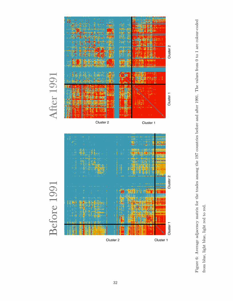
Fig

ure

6:A

ver

age

ad

jace

ncy

mat

rix

for

the

trad

esam

ong

the

197

cou

ntr

ies

bef

ore

and

afte

r19

91.

Th

eva

lues

from

0to

1ar

eco

lou

r-co

ded

from

blu

e,ligh

tb

lue,

light

red

tore

d.

32

However a more fertile exploration is perhaps to extend the setting for non-Erdos-Renyi networks,

incorporating in the model some stylized features of network data such as transitivity, homophily.

The development in this direction will be reported in a follow-up paper. On the other hand,

dynamic networks with weighted edges may be treated as matrix time series for which effective

modelling procedures have been developed based on various tensor decompositions (Wang et al.,

2019; Chang et al., 2020a).

References

Aggarwal, C. and Subbian, K. (2014). Evolutionary network analysis: A survey. ACM ComputingSurveys (CSUR), 47(1):1–36.

Barbieri, K. and Keshk, O. M. G. (2016). Correlates of War Project Trade Data Set Codebook,Version 4.0. Online: http://correlatesofwar.org.

Barbieri, K., Keshk, O. M. G., and Pollins, B. (2009). Trading data: Evaluating our assumptionsand coding rules. Conflict Management and Peace Science, 26(5):471–491.

Bennett, G. (1962). Probability inequalities for the sum of independent random variables. Journalof the American Statistical Association, 57(297):33–45.

Bhattacharjee, M., Banerjee, M., and Michailidis, G. (2020). Change point estimation in a dy-namic stochastic block model. Journal of Machine Learning Research, 21(107):1–59.

Bradley, R. C. (2007). Introduction to strong mixing conditions. Kendrick press.

Chang, J., He, J., and Yao, Q. (2020a). Modelling matrix time series via a tensor cp-decomposition. Under preparation.

Chang, J., Kolaczyk, E. D., and Yao, Q. (2020b). Discussion of “network cross-validation by edgesampling”. Biometrika, 107(2):277–280.

Chang, J., Kolaczyk, E. D., and Yao, Q. (2020c). Estimation of subgraph densities in noisynetworks. Journal of the American Statistical Association, (In press):1–40.

Chen, E. Y., Fan, J., and Zhu, X. (2020). Community network auto-regression for high-dimensional time series. arXiv:2007.05521.

Crane, H. et al. (2016). Dynamic random networks and their graph limits. The Annals of AppliedProbability, 26(2):691–721.

Donnat, C. and Holmes, S. (2018). Tracking network dynamics: A survey of distances andsimilarity metrics. The Annals of Applied Statistics, 12(2):971–1012.

Durante, D., Dunson, D. B., et al. (2016). Locally adaptive dynamic networks. The Annals ofApplied Statistics, 10(4):2203–2232.

Durrett, R. (2019). Probability: theory and examples, volume 49. Cambridge university press.

Fan, J. and Yao, Q. (2003). Nonlinear Time Series: Nonparametric and Parametric Methods.Springer, New York.

33

Fu, W., Song, L., and Xing, E. P. (2009). Dynamic mixed membership blockmodel for evolvingnetworks. In Proceedings of the 26th Annual International Conference on Machine Learning,pages 329–336.

Hanneke, S., Fu, W., and Xing, E. P. (2010). Discrete temporal models of social networks.Electronic Journal of Statistics, 4:585–605.

Kang, X., Ganguly, A., and Kolaczyk, E. D. (2017). Dynamic networks with multi-scale temporalstructure. arXiv preprint arXiv:1712.08586.

Kolaczyk, E. D. (2017). Topics at the Frontier of Statistics and Network Analysis. CambridgeUniversity Press.

Krivitsky, P. N. and Handcock, M. S. (2014). A separable model for dynamic networks. Journalof the Royal Statistical Society, B, 76(1):29.

Lin, Z. and Bai, Z. (2011). Probability inequalities. Springer Science & Business Media.

Ludkin, M., Eckley, I., and Neal, P. (2018). Dynamic stochastic block models: parameter estima-tion and detection of changes in community structure. Statistics and Computing, 28(6):1201–1213.

Mastrandrea, R., Fournet, J., and Barrat, A. (2015). Contact patterns in a high school: A com-parison between data collected using wearable sensors, contact diaries and friendship surveys.PLoS ONE, 10(9):e0136497.

Matias, C. and Miele, V. (2017). Statistical clustering of temporal networks through a dynamicstochastic block model. Journal of the Royal Statistical Society, B, 79(4):1119–1141.

Merlevede, F., Peligrad, M., Rio, E., et al. (2009). Bernstein inequality and moderate deviationsunder strong mixing conditions. In High dimensional probability V: the Luminy volume, pages273–292. Institute of Mathematical Statistics.

Pensky, M. (2019). Dynamic network models and graphon estimation. Annals of Statistics,47(4):2378–2403.

Rohe, K., Chatterjee, S., Yu, B., et al. (2011). Spectral clustering and the high-dimensionalstochastic blockmodel. The Annals of Statistics, 39(4):1878–1915.

Vanhems, P., Barrat, A., Cattuto, C., Pinton, J.-F., Khanafer, N., Regis, C., a. Kim, B., andB. Comte, N. V. (2013). Estimating potential infection transmission routes in hospital wardsusing wearable proximity sensors. PloS ONE, 8:e73970.

Vinh, N. X., Epps, J., and Bailey, J. (2010). Information theoretic measures for clusteringscomparison: Variants, properties, normalization and correction for chance. Journal of MachineLearning Research, 11:2837–2854.

Wang, D., Liu, X., and Chen, R. (2019). Factor models for matrix-valued high-dimensional timeseries. Journal of Econometrics, 208(1):231–248.

Wang, D., Yu, Y., and Rinaldo, A. (2018). Optimal change point detection and localization insparse dynamic networks. arXiv preprint arXiv:1809.09602.

Wilson, J. D., Stevens, N. T., and Woodall, W. H. (2019). Modeling and detecting change intemporal networks via the degree corrected stochastic block model. Quality and ReliabilityEngineering International, 35(5):1363–1378.

34

Xu, K. S. and Hero, A. O. (2014). Dynamic stochastic blockmodels for time-evolving socialnetworks. IEEE Journal of Selected Topics in Signal Processing, 8(4):552–562.

Yang, T., Chi, Y., Zhu, S., Gong, Y., and Jin, R. (2011). Detecting communities and theirevolutions in dynamic social networks?a bayesian approach. Machine learning, 82(2):157–189.

Yu, Y., Wang, T., and Samworth, R. J. (2015). A useful variant of the davis–kahan theorem forstatisticians. Biometrika, 102(2):315–323.

Zhao, Z., Chen, L., and Lin, L. (2019). Change-point detection in dynamic networks via graphonestimation. arXiv preprint arXiv:1908.01823.

Zhu, T., Li, P., Yu, L., Chen, K., and Chen, Y. (2020a). Change point detection in dynamicnetworks based on community identification. IEEE Transactions on Network Science and En-gineering.

Zhu, X., Huang, D., Pan, R., and Wang, H. (2020b). Multivariate spatial autoregressive modelfor large scale social networks. Journal of Econometrics, 215(2):591–606.

Zhu, X., Pan, R., Li, G., Liu, Y., and Wang, H. (2017). Network vector autoregression. TheAnnals of Statistics, 45(3):1096–1123.

Zhu, X., Wang, W., Wang, H., and Hardle, W. K. (2019). Network quantile autoregression.Journal of Econometrics, 212(1):345–358.

35