Automotive core tool: MSA -...

Everyone is muted. We will start at 7pm EST.

Automotive core tool: MSA

Kush Shah, ChairmanASQ Automotive Division

• Housekeeping Items

• About ASQ Automotive Division

• Our Vision

• Webinar Series

• Automotive core tool: MSA

• Questions & Answers

Agenda

Everyone is muted

Session is being recorded

Session will last about 90 minutes

ASQ Automotive members can download the slides

and video at www.asq-auto.org

Participate thru chat and questions

Will answer questions at the end:• Q&A at the end of the presentation

• Please type your questions in the panel box

Housekeeping Items

• Manager, Global Electrification, General Motors,

Michigan, U.S.

• Leadership positions in Engineering, R&D,

Manufacturing, Quality

• 20+ years of quality experience

• Six Sigma Master Black Belt, Shainin Red X

Master, ASQ CQA, CMQ/OE,CQE, CSSBB

• Speaker at International Quality Symposiums /

Conferences

• Trainer for Six Sigma and Quality Management

About Me

ASQ Automotive Chair

Kush Shah

Global Automobile Outlook – 2020

>1 billion vehicles - Circle the earth 125 times

~3% annual growth worldwide

15% ownership

American Society for Quality (ASQ):ASQ is the world's leading professional association and authority on quality

ASQ Automotive Division Mission:To be the recognized global network of automotive quality professionals that is helping individuals and organizations to achieve personal and organizational excellence

Key Objectives of ASQ Automotive Division:

Increase Member Value – Webinars, symposium and Automotive Excellence magazine

Develop Core Tools Competency –On-site training -PPAP, APQP, FMEA, SPC and MSA

Global Outreach – Participate in conferences and deliver training globally

Key Objectives of ASQ Automotive Division:

U.S. Outreach - Engage all automotive OEMs and Tier 1 & 2 suppliers

Student Outreach – Collaborate with universities

Collaborate With Other Professional Societies –Engage with other societies and professional organizations

Core Quality Tools for Automotive Industry:

Advanced Product Quality Planning (APQP)Failure Mode and Effects Analysis (FMEA)Production Part Approval Process (PPAP)

Measurement Systems Analysis (MSA) Statistical Process Control (SPC)

ASQ Automotive Division provides on-site training by certified instructors.

The ASQ Automotive Division is pleased to present a

regular series of free webinars featuring leading

international experts, practitioners, academics, and

consultants. The goal is to provide a forum for the

continuing education of automotive professionals.

ASQ Automotive members can

download the presentation slides on

our website www.asq-auto.org.

Recorded webinars are also

available for viewing after the events

for members.

Resources / Contacts:

Contact: Kush Shah, Chair - ASQ Automotive Division

E-mail : [email protected]

Website: www.asq-auto.org

Group: ASQ Automotive Division Group

twitter.com/ASQautomotive

Mark A. Morris has more than 30 years experience in tooling and

manufacturing as a skilled machinist, toolmaker, college instructor,

technical writer, and quality professional in roles from Quality Engineer

to Director of Continuous Improvement. His expertise lies in

dimensional issues, reliability, maintainability, and quality systems. Mr.

Morris’ credentials include undergraduate degrees focused on

manufacturing engineering, industrial education, and metalworking;

Master of Education degree from the College of Technology at Bowling

Green State University; CQE, CRE, and CQA certifications from the

American Society for Quality; and Senior Level Geometric Dimensioning

and Tolerancing Professional (GDTP) certification from the American

Society of Mechanical Engineers. Mr. Morris is also the Immediate Past

Chair for the Ann Arbor section of ASQ, and for the past five years, has

trained candidates to become ASQ Certified Quality Engineers. He

presently serves as Education Chair on the Leadership Team of the Ann

Arbor section of ASQ..

Mark A. Morris

Measurement Systems Analysis

based on MSA 4th Edition

Mark A. Morris

ASQ Automotive Division Webinar

January 25, 2012

[email protected]

Agenda

1. Quality Statistics Review

2. Fundamental MSA Concepts

3. Preparation for MSA Studies

4. Mathematics of MSA Studies

5. Evaluation of MSA Studies

6. Summary and Closure

Course Goals

1. To provide a fundamental understanding of the

language that guides MSA studies.

2. To use MSA studies to determine where

measurement processes require improvement

to assess special characteristics.

3. To achieve robust capable measurement

processes for special characteristics.

Quality Statistics Review

We Need Operational Definitions

“Without an operational definition, investigations of a problem will be costly and ineffective, almost certain to lead to endless bickering and controversy.”

W. Edwards Deming, Ph.D.

Operational definitions provide three components:

1. Specify Test to determine Compliance

2. Set Criteria for Judgment

3. Make Decisions based on the Criteria

Feature Control Frames

• Feature Control Frame is a rectangular symbol that

consists of two to five compartments, used to specify

geometric tolerances:

– First compartment specifies the geometric characteristic.

– Second compartment specifies the tolerance value.

– Third compartment, if it exists, specifies the primary datum.

– Fourth compartment, if it exists, specifies the second datum.

– Fifth compartment, if it exists, specifies the third datum.

Use of Basic Dimensions

• Basic dimensions define the perfect location of features and surfaces relative to the datum reference frame.

• Basic dimensions are used to define the theoretical exact size and location for features.

• Feature control frames define the intended tolerance for features.

A Datum Reference Frame

• Three mutually perpendicular planes.

DatumPoint

3 Datum Planesdefine the Originof Measurement

X

Z

Y

Datum Feature Simulators

• In the real world, we use physical datum feature

simulators to establish datums:

– Machine Tool Elements

– Surface Plates

– Angle Plates

• Manufactured parts have irregularities.

• High points on parts make contact with datum

feature simulators to establish datums.

2009

Datum Schemes

Note: The backsurface is datum A.

Datum Schemes

A Fundamental Concept

“No two things are alike, but even if they

were, we would still get different values

when we measured them.”Donald J Wheeler, Ph.D.

Variation in All Things

Individual Measurements

Natural Process Variation

More Measurements

More Measurements

Natural Variation Inherent in the Process

Environment

Equipment

Material

Methods

People

Causes and Effects

EnvironmentEquipment

Material

Methods

People

Result

Changes in Behavior

Original Distribution Change in Location

Change in Dispersion Change in Shape

Purpose of SPC

• The purpose of SPC is to understand the

behavior of a process.

• The goal of that understanding is to predict how

the process may perform in the future.

• All, so we may take appropriate action.

A Philosophy of Actionable Data

� No Inspection without Recording

� No Recording without Analysis

� No Analysis without ActionW. Edwards Deming, Ph.D.

Time

Some Processes are Predictable

• Absence of Unexpected Changes

• Common Cause Variation

• In Statistical Control

• Process is Stable

Time

Other Processes Lack Stability

• Presence of Unexpected Changes

• Special Causes are Present

• Significant Changes Occur

• Process Out of Control

• Unstable

X Chart

Range Chart

Control Chart Shows Stability

Partial Drawing of a Shaft

In this example we are going to look at the width of the keyway in the view above.

X-bar and R with Gage R&R Data

And Another Thing…

“If you are responsible for a measurement

process, and you are not monitoring that

process on a control chart, then you are not

doing your job!!!”Emil Jebe, Ph.D.

Purpose of Control Charts

Action Taken No Action Taken

Action Required

Good

Sin of

Omission

No Action Required Sin of

Commission Good

Measurement Systems Analysis

• Bias

• Linearity

• Stability

• Repeatability

• Reproducibility

Target Practice

Accuracy and Precision

Accurate and Precise Accurate but not Precise

Precise but not Accurate Neither Precise nor Accurate

Resolution

LSL USL

2 Increments or less � Inadequate

4 Increments � Minimum for Pre-Control

10 Increments � Minimum Recommended

Note: The MSA Guideline recommends a minimum of five distinct categories compared to the process distribution for control and analysis activities.

Linearity

• Linearity is the difference in the bias values through the expected operating range of the gage.

Larger

Positive BiasSmaller

Positive Bias

Stability

• Stability is the range between the largest and smallest bias from two or more sets of measurements taken over time.

Stability

Time 2

Time 1

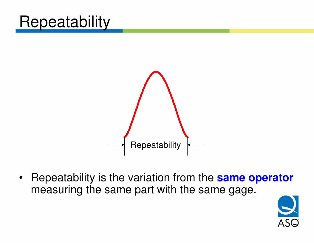
Repeatability

• Repeatability is the variation from the same operatormeasuring the same part with the same gage.

Repeatability

Reproducibility

• Reproducibility is the variation from different operators measuring the same part with the same gage. Operator A

Operator B

Operator C

Reproducibility

Purpose of Inspection

Accept Parts Reject Parts

Good Parts

Good Excess Cost

Bad Parts Upset Customers and Higher

Cost

Good

Measurement Error in Measurements

Small MeasurementVariation

Large MeasurementVariation

Process Variation

Process Variation

Small Measurement Error Provides

Better Information on the Process

Small MeasurementVariation

Large MeasurementVariation

Process Variation

Process Variation

Measured Variation

Measured Variation

Impact of Measurement Uncertainty

TargetValue

LowerSpecification

Limit

UpperSpecification

Limit

Potential to Accept Bad Parts

Potential to Reject Good Parts

Statistical Problem Solving

A three-step process for problem solving:

1. Identify and remove causes of instability.

2. Identify and correct causes of too much variation.

3. Identify and correct causes of off-target conditions.

Hans Bajaria, Ph.D.

Fundamental MSA Concepts

Fundamental MSA Concepts

Order of Presentation

Purpose of MSA Studies

Common Use of Terms

Requirements for Inspection

Measurement as a Process

Measurement System Planning

Measurement System Development

Quantification of Measurement Error

Measurement System Uncertainty

Common Use of MSA Terms

• Measurement allows us to assign numbers to material things to describe specific properties.– Measurement Process

– Measured Value

• A Gage is any device used to obtain measurements, including attribute devices.

• Measurement System is the collection of instruments, gages, standards, methods, fixtures, software, personnel, environment, and assumptions used to quantify measurements.

A Measurement Ensemble

Measurements

Associated Equipment

Instruments

Artifacts

Standards

PersonnelProcedures

All the influences that affect uncertainty ofcalibrations and measurements

Note: The item being measured is outside the scope of the measurement ensemble.

Standard

• Accepted as the Basis for Comparison

• Provides the Criteria for Acceptance

• A Known Value (within limits of uncertainty)

A standard should be used within the context of an

operational definition, to yield the same results with

the same meaning yesterday, today, and tomorrow.

Basic Equipment

• Discrimination, Readability, Resolution

– Smallest unit of measure for an instrument.

• Effective Resolution

– Sensitivity of a gage for a particular application.

• Reference Value

– The accepted value for an artifact.

• True Value

– The actual value for an artifact. (unknown and unknowable)

Location Variation

• Accuracy

– Closeness to the true value.

• Bias

– Systematic error in the measurement process.

• Stability

– Change in bias over time.

• Linearity

– Change in bias in the normal operating range.

Width Variation

• Precision

• Repeatability

• Reproducibility

• GRR or Gage R&R

• Measurement System Capability

• Measurement System Performance

System Variation

• Capability

– Variability in the short-term.

• Performance

– Variability in the long-term. (estimate of total variability)

• Uncertainty

– The MSA Guideline uses this term to describe a tolerance

interval for measured values.

Note: The measurement system must be both stable and consistent.

Standards and Traceability

• It is appropriate to differentiate between the

National Reference Standards and the National

Institute of Standards and Technology where they

are maintained.

• The key concept of traceability requires calibration

of measurement devices through an unbroken

chain of comparisons, all having known

uncertainties.

Purpose of Inspection

Accept Parts Reject Parts

Good Parts

Good Excess Cost

Bad Parts Upset Customers and Higher

Cost

Good

Properties of Measurement Systems

• Adequate Discrimination and Sensitivity

– Increments of measure should be small compared to

the specification limits for Product Control.

– Increments of measure should be small compared to

the process variation for Process Control.

• Measurement System in Statistical Control

– The Random Effects model is essential.

– Otherwise, a measurement process does not exist,

according to Dr. Deming. (Out of the Crisis, 1986, p. 280)

Impact of Variability on Product Control

TargetValue

LowerSpecification

Limit

UpperSpecification

Limit

Potential to Accept Bad Parts

Potential to Reject Good Parts

Impact of Variability on Process Control

• Measurement variability can lead us to act when we

should not, or to not act when we should.

Action Taken No Action

Taken

Action Required

Good

Sin of

Omission

No Action

Required

Sin of

Commission Good

A Tale of Two Technicians

Technician 1

• Careful his instrument was always calibrated.

• Every hour he checked his gage against the

standard.

• If it did not read zero, he reset the gage to zero.

• Because of this hourly recalibration, Technician 1

was considered to be a very careful and

conscientious worker.

Based on the thoughts of Wheeler and Lyday


Technician 2

• Technician 2 used the same instrument.

• Every hour he checked his gage against the standard, but recorded the reading on a control chart.

• Instead of making hourly adjustments to the gage, he only adjusted the instrument when the value showed a lack of control.

• Otherwise, he continued to use the gage without adjustment.


• The two technicians continued to operate in this

manner for several months.

• Finally, when their supervisor became aware of the

different methods being used, she decided to study

the results of the two methods.

• She created histograms that showed the amount of

variation that the two technicians had recorded

during their hourly calibrations.

• The scale shows variation from zero.


0 2 4 6 8 10 12-2-4-6 0 2 4 6-2-4-6

Technician 1 Technician 2


• Hourly adjustments by Technician 1 made the

histogram wider.

• The variation of his adjustments was added to the

natural variation of the measurements themselves.

• Many of the adjustments made by Technician 1 were

unnecessary, and every one of them added to the

variation seen in the wider histogram.


• Technician 2, on the other hand, had a narrower

histogram because he only adjusted the gage when

the control chart gave a clear signal of the need to

adjust.

• In fact, Technician 2 rarely made any adjustments to

the gage except at the beginning of his shift.

• The histogram suggests that these adjustments were

necessary to undo the needless adjustments of

Technician 1.


• Based on this study, a new calibration procedure was

adopted.

• Control charts were made a routine part of every

calibration scheme, and the standard operating

procedure was changed so that adjustments would

only be made in response to lack of control.

• Several of the company’s test methods showed an

immediate and dramatic improvement due to the

elimination of over-calibration.


• Use of a control chart to check the consistency of a

measurement process provides a scientific signal when

recalibration is necessary.

Action Taken No Action

Taken

Action Required

Good

Sin of

Omission

No Action

Required

Sin of

Commission Good

Preparation for MSA Studies

Statement of the Problem

“A problem well defined is half solved.”John Dewey, Ph.D.

“The formulation of a problem is far more often essential

than its solution, which may be merely a matter of

mathematical or experimental skill.”Albert Einstein, Ph.D.

Two Important Questions

• Are we measuring the correct variable at the correct

location?

– If the wrong variable is measured, then regardless of the

accuracy and precision, we will simply spend money with

no benefit.

• What statistical properties does the measurement

process need to demonstrate to demonstrate that it is

adequate?

– These properties will guide the MSA study.

Preparing for the MSA Study

1. Plan the approach for the MSA study.

2. Select number of parts, appraisers, and trials.

3. Select appraisers from real operators.

4. Select parts that represent the process.

– Select parts to represent the operating range.

– If parts do not represent the total operating range, then you must ignore TV in the study.

5. Verify the gage has adequate discrimination.

6. Assure that the methods are clearly defined.

Mathematics of MSA Studies

One Method to Assess Stability

1. Obtain a sample and establish its reference value

relative to a traceable standard.

2. On a periodic basis, measure the master sample

three to five times.

3. Record the data and plot the data on an X-bar & R

chart or an X-bar & s chart.

Assessing Bias – Independent Sample

1. Obtain a sample and establish its reference value

relative to a traceable standard.

2. Have a single appraiser measure the sample a

predetermined number of times (n > 10).

3. Plot a histogram and review the graphical results.

Assessing Bias – Independent Samples

6.05.95.85.75.6 6.1 6.2 6.3 6.4

Assessing Bias – Independent Sample

4. Compute the average of the n measurements.

5. Compute the repeatability standard deviation.

6. Determine the t statistic for the bias.

7. Bias is acceptable if the α level if zero is contained

within the 1-α confidence bounds.

Assessing Bias – Control Chart Method

If a control chart is used to monitor stability of the measurement process, this data can also be used to evaluate bias.

1. Obtain a sample and establish its reference value relative to a traceable standard.

2. Plot a histogram and review the graphical results.

Methods to Assess Linearity

1. Select at least 5 parts with measured values that

cover the operating range of the gage.

2. Have each of the parts measured to determine

reference a value for each.

3. Measure each part at least 10 times to assess

linearity of the gage in question.

Range Method for Gage R&R

Number of Parts 5

Number of Appraisers 2

Processs Standard Deviation (from previous study) 0.0777

Acceptable GRR Less Than 10%

Unacceptable GRR Greater than 30%

Repeatability and Roproducibility

Range Method

MSA 3rd Edition Chapter 3 Section B Page 97-98

User Setup

Repeatability and ReproducibilityRange Method

MSA 4th Edition, Chapter 3, Section B, Pages 102 – 103User Setup


Parts Appraiser A Appraiser B Appraiser C

1 0.85 0.80

2 0.75 0.70

3 1.00 0.95

4 0.45 0.55

5 0.50 0.60

6

7

8

9

10


Range Method


Data Input

Repeatability and ReproducibilityRange Method

MSA 4th Edition, Chapter 3, Section B, Pages 102 – 103Data Input

Range Method for Gage R&RParts Appraiser A Appraiser B Appraiser C Range

1 0.85 0.80 0.05

2 0.75 0.70 0.05

3 1.00 0.95 0.05

4 0.45 0.55 0.10

5 0.50 0.60 0.10

6 -

7 -

8 -

9 -

10 -

Average Range (R-bar) 0.070

d*2 1.19

GRR 0.0588

Process Standard Deviation (from previous study) 0.0777

%GRR 75.64%




d*2Parts (g) 2 3

1 1.41421 1.91155

2 1.27931 1.80538

3 1.23105 1.76858

4 1.20621 1.74989

5 1.19105 1.73857

6 1.18083 1.73099

7 1.17348 1.72555

8 1.16794 1.72147

9 1.16361 1.71828

10 1.16014 1.71573

Source: Appendix C page 195

Constants d*2 1.19105

Appraisers (m)

Constant Tables

Source: Appendix C, Page 203

Average & Range Method – Gage R&R

Number of Parts 10

Number of Appraisers 3

Number of Trials 3



Acceptable Number of Distinct Categories 5

User Setup


Average and Range Method

Repeatability and RoproducibilityRepeatability and ReproducibilityAverage and Range Method

MSA 4th Edition, Chapter 3, Section B, Pages 103 – 119User Setup


PART DESCRIPTION Item #45

CHARACTERISTIC Surface Friction

SPECIFICATION - NOMINAL 0.96

SPECIFICATION - LOWER LIMIT (LSL) 0.46

SPECIFICATION - UPPER LIMIT (USL) 1.46

GAUGE NAME: Instron

GAUGE #: 1645

GAUGE TYPE: SF Gage

DATE 21-Feb-03

ANALYSIS PERFORMED BY Bev

User: Enter Data only in Yellow Boxes Example:


PART DESCRIPTION: GAUGE NAME: DATE: 21-Feb-03

CHARACTERISTIC: GAUGE #: PERFORMED BY:

SPECIFICATION: 0.96 + 0.5 - 0.5 GAUGE TYPE:

DATA

Appraiser a:(NAME)=

PART

TRIAL # 1 2 3 4 5 6 7 8 9 10

1 0.2900 -0.5600 1.3400 0.4700 -0.8000 0.0200 0.5900 -0.3100 2.2600 -1.3600

2 0.4100 -0.6800 1.1700 0.5000 -0.9200 -0.1100 0.7500 -0.2000 1.9900 -1.2500

3 0.6400 -0.5800 1.2700 0.6400 -0.8400 -0.2100 0.6600 -0.1700 2.0100 -1.3100

Appraiser b:(NAME)=

PART

TRIAL # 1 2 3 4 5 6 7 8 9 10

1 0.0800 -0.4700 1.1900 0.0100 -0.5600 -0.2000 0.4700 -0.6300 1.8000 -1.6800

2 0.2500 -1.2200 0.9400 1.0300 -1.2000 0.2200 0.5500 0.0800 2.1200 -1.6200

3 0.0700 -0.6800 1.3400 0.2000 -1.2800 0.0600 0.8300 -0.3400 2.1900 -1.5000

Appraiser c:(NAME)=

PART

TRIAL # 1 2 3 4 5 6 7 8 9 10

1 0.0400 -1.3800 0.8800 0.1400 -1.4600 -0.2900 0.0200 -0.4600 1.7700 -1.4900

2 -0.1100 -1.1300 1.0900 0.2000 -1.0700 -0.6700 0.0100 -0.5600 1.4500 -1.7700

3 -0.1500 -0.9600 0.6700 0.1100 -1.4500 -0.4900 0.2100 -0.4900 1.8700 -2.1600

Reference Value 1.0800 1.1000 1.0600 1.1000 1.0000 1.3340 1.3320 1.0800 0.9960 1.0020

Greg

Rob

Bill

Item #45

Surface Friction 1645

Instron

SF Gage Bev


Number of averages falling outside control limits 22

Percent of averages falling outside control limits 73%

Number of Ranges falling outside control limits 1

There are differences between the variability of the appraisers.


Average and Range Method


Results

Repeatability and ReproducibilityAverage and Range Method

MSA 4th Edition, Chapter 3, Section B, Pages 103 – 119Results

Evaluation of MSA Studies

Analysis of Results for Stability

• Review range chart for adequate discrimination.

• Establish control limits and review range control

chart for out-of-control signals.

• Take appropriate action when the range chart goes

out-of-control.

Analysis of Gage R&R Results

Average Chart -- "Stacked"

-2.500

-2.000

-1.500

-1.000

-0.500

0.000

0.500

1.000

1.500

2.000

2.500

1 2 3 4 5 6 7 8 9 10

Part

Av

era

ge

Ap A Ap B Ap C UCL LCL Average


Average Chart -- "Unstacked"

-2.500

-2.000

-1.500

-1.000

-0.500

0.000

0.500

1.000

1.500

2.000

2.500

A1

A2

A3

A4

A5

A6

A7

A8

A9

A10

B1

B2

B3

B4

B5

B6

B7

B8

B9

B10

C1

C2

C3

C4

C5

C6

C7

C8

C9

C10

Appraiser / Part

Av

era

ge

A/P Avg UCL LCL Average


Range Chart -- "Stacked"

0.000

0.200

0.400

0.600

0.800

1.000

1.200

1 2 3 4 5 6 7 8 9 10

Part

Ra

ng

e

Ap A Ap B Ap C UCL R Avg Range


Range Chart "Unstacked"

0.000

0.200

0.400

0.600

0.800

1.000

1.200

A1

A2

A3

A4

A5

A6

A7

A8

A9

A10

B1

B2

B3

B4

B5

B6

B7

B8

B9

B10

C1

C2

C3

C4

C5

C6

C7

C8

C9

C10

Appraiser / Part

Ran

ge

A/P Range UCLR Avg Range


Scatter Plot

-2.500

-2.000

-1.500

-1.000

-0.500

0.000

0.500

1.000

1.500

2.000

2.500

1A

1B

1C 2A

2B

2C 3A

3B

3C 4A

4B

4C 5A

5B

5C 6A

6B

6C 7A

7B

7C 8A

8B

8C 9A

9B

9C

10A

10B

10C

Part - Appraiser - Trial

Va

lue

Appr A Appr B Appr C


Error Chart based on Average Measurement

-0.800

-0.600

-0.400

-0.200

0.000

0.200

0.400

0.600

0.800

1A

1B

1C 2A

2B

2C 3A

3B

3C 4A

4B

4C 5A

5B

5C 6A

6B

6C 7A

7B

7C 8A

8B

8C 9A

9B

9C

10A

10B

10

C

Part - Appraiser - Trial

Err

or

Appr A Appr B Appr C

Measurement Problem Analysis

A three-step process for problem solving:

1. Identify and remove causes of instability.

2. Identify and correct causes of too much variation.

3. Identify and correct causes of off-target conditions.

Hans Bajaria, Ph.D.

Summary and Closure

Course Goals

1. To provide a fundamental understanding of the

language that guides MSA studies.

2. To use MSA studies to determine where

measurement processes require improvement

to assess special characteristics.

3. To achieve robust capable measurement

processes for special characteristics.

Questions and Answers

Please type your

questions in the panel

box

Thank You For AttendingPlease visit our website www.asq-auto.org for future webinar dates and topics.

Automotive core tool: MSA -...

Documents

Transcript of Automotive core tool: MSA -...