
Automating ISO 26262 Hardware Evaluation …...For the development of hardware systems, ISO 26262...
132
Faculdade de Engenharia da Universidade do Porto Automating ISO 26262 Hardware Evaluation Methodologies João Manuel Cardoso Tavares Dissertation Developed under the Scope of the Integrated Master in Electrical and Computers Engineering Major Automation Supervisor: David Parker (PhD), University of Hull Co-Supervisor: Rui Esteves Araújo (PhD) July, 2014
Transcript of Automating ISO 26262 Hardware Evaluation …...For the development of hardware systems, ISO 26262...
Faculdade de Engenharia da Universidade do Porto
Automating ISO 26262 Hardware Evaluation Methodologies
João Manuel Cardoso Tavares
Dissertation Developed under the Scope of the
Integrated Master in Electrical and Computers Engineering
Major Automation
Supervisor: David Parker (PhD), University of Hull
Co-Supervisor: Rui Esteves Araújo (PhD)
July, 2014

II Problem

© João Tavares, 2014
IV Problem
Abstract
The constant evolution of vehicles, incorporating more commodities and functionalities,
has been made possible by electric, electronic and programmable electronic components. To
assure the reliability of the safety-related systems that use those components, functional safety
standards are created to define processes and guidelines for their development. Some of those
systems control important functions such as steering and braking in road vehicles. For that
purpose, the Automotive Functional Safety Standard, ISO 26262, was launched.
Manual Safety Analysis for complex electronic systems can be a difficult and time-
demanding task, with no assurance of success, as it is error prone. With that in mind, the
University of Hull developed a safety and reliability tool, to automate some of the safety
analysis steps. Hierarchically-Performed Hazard Origin and Propagation Studies (HiP-HOPS) is
that state-of-the-art tool.
For the development of hardware systems, ISO 26262 proposes a set of evaluation metrics,
which can be used to compare system’s designs. Furthermore, it guides the designer through
the process of choosing safety mechanisms to assure the targets for those metrics are achieved.
Currently, the safety analysis that is being done using HiP-HOPS does not consider those safety
mechanisms. It also does not perform the metrics calculation.
The aim of this thesis is to extend HiP-HOPS capabilities, so it can incorporate those safety
mechanisms and perform metrics calculations automatically, to allow the user to test different
hardware implementations and point to the best solution.
The topics here stated, namely safety analysis, HiP-HOPS and the standard ISO 26262, are
explored in the firstly looked at Literature Review. Then, the changes made to HiP-HOPS are
explained and validated through the analysis of a chosen hardware system. The last part is
dedicated to result analysis, final considerations and further developments on the metrics
software program.

VI Problem
Resumo
A evolução constante dos veículos, incorporando mais comodidades e funcionalidades, tem
sido possível graças a componentes elétricos, eletrónicos e de eletrónica programável. De modo
a assegurar a fiabilidade de sistemas relacionados com segurança que usam esses componentes,
normas de segurança funcional têm sido criadas para definir processos e metodologias para o
seu desenvolvimento. Alguns desses sistemas controlam funções importantes como direção e
travagem em automóveis. Para esse propósito, a norma de segurança funcional automóvel, ISO
26262, foi lançada.
Realizar análise de segurança manualmente, em sistemas eletrónicos complexos, pode ser
uma tarefa difícil e demorada, sem garantia de sucesso, visto que é suscetível ao erro humano.
Com esta problemática em mente, a University of Hull desenvolveu uma ferramenta de
segurança e fiabilidade, para automatizar algumas das etapas da análise de segurança. Essa
ferramenta designa-se por Hierarchically-Performed Hazard Origin and Propagation Studies
(HiP-HOPS).
Para o desenvolvimento de sistemas de hardware, a norma ISO 26262 propõe um conjunto
de métricas de avaliação que são utilizadas para comparar diferentes implementações. Além
disso, guia o utilizador ao longo de um processo de escolha de mecanismos de segurança que
permitem assegurar o cumprimento dos objetivos quantitativos das métricas. Neste momento,
a análise de segurança feita através do HiP-HOPS não tem em consideração esses mecanismos
de segurança, nem faz o cálculo das métricas.
O objetivo desta tese é extender as capacidades do HiP-HOPS, de modo a incorporar os
mecanismos de segurança na sua análise e fazer o cálculo das métricas automaticamente, de
forma a permitir que o utilizador teste implementações de hardware diferentes e apontá-lo na
direção da melhor solução.
Os tópicos aqui mencionados, nomeadamente análise de segurança, a ferramenta HiP-HOPS
e a norma ISO 26262, serão explorados na revisão de literatura. Seguidamente, as mudanças
feitas no HiP-HOPS serão explicadas e validadas através da análise do sistema de hardware
escolhido. A última parte será dedicada à análise dos resultados obtidos, às considerações finais
e a futuros desenvolvimentos do software para as métricas.


VIII Problem
Acknowledgments
First, I would like to express my gratitude towards Rui Esteves, PhD, my supervisor at
Faculdade de Engenharia da Universidade do Porto. He granted me the opportunity to work on
this thesis and was, always, a fantastic guiding voice and valuable help throughout this
adventure.
I am equally grateful to David Parker, PhD, my supervisor with the University of Hull. From
the first day he was incredibly supportive and gave me critical advice and help which was key
to successfully complete this thesis.
My very special thanks goes to Luís Azevedo, PhD student at the University of Hull. He was
the force that carried me, everyday, through the difficulties of the project. I will never forget
his fantastic guidance and friendship.
I would also like to acknowledge my friends Carina Treffurth and Sara Teter for their
amazing work as editors on this thesis.
A special cheers to all the friends I met in Hull. Distinctively to my Family at 80-82
Cottingham Road (and Guests) and the Portuguese Crew. Rémi, Lucas, Carina, Katie, Simone,
Sara, Sarah, Till, Simon, Marie, Anke, João, Franciscos, Hélène, Bernardo, Pedro, Tiago, you
were the ones that made this semester abroad an unforgettable experience. And thanks for
giving me infinite reasons not to work on my thesis. “Come on…Make good choices”.
To all my friends in Portugal, I thank you for accompanying me throughout my life. You are
the reason why it has been amazing.
To my beloved family, I am infinitely grateful. My father, mother, sisters, grandparents and
remaining family are the most important people in my life and the ones that shaped me into
the person I am today.
To my dearest friend and companion, Manuel Tavares, my grandfather, I dedicate my most
special thanks. Thank you for all the advice, support, patience, confidence and friendship. I
just hope that one day I become half the man you were.
This thesis is dedicated to all of you,
João Tavares

X Problem
Contents
ABSTRACT IV
RESUMO VI
ACKNOWLEDGMENTS VIII
LIST OF FIGURES XII
LIST OF TABLES XV
SYMBOLS AND ABBREVIATIONS XVII
CHAPTER 1 1
INTRODUCTION 1
1.1. Problem 1
1.2. Thesis’ Aim 1
1.3. Document Outline 2
CHAPTER 2 4
LITERATURE AND CONCEPTS REVIEW 4
2.1. Functional Safety and SILs 4
2.2. ISO 26262 6
2.3. Classic safety analysis techniques: FTA and FMEA 9
2.4. Modern Safety Analysis Tools and Techniques 10
2.5. Automatic optimization of system reliability 11
2.6. HiP-HOPS and Safety Analysis 12
2.7. Summary 22
CHAPTER 3 23
HARDWARE EVALUATION TECHNIQUES 23
3.1. Introduction 23
3.2. Safety Mechanisms 24
3.3. Fault classification of a hardware element 29
3.4. ISO 26262 Hardware Metrics 31
3.5. Evaluation of Safety Goal Violations 35
3.6. Automatic Evaluation Techniques with HiP-HOPS 39
3.7. Summary 43
CHAPTER 4 45
IMPLEMENTATION OF THE HARDWARE EVALUATION TECHNIQUES 45
4.1. ECU circuit example 45
4.2. System Failures Annotation 49
4.3. Safety Analysis 58
4.4. HiP-HOPS Safety Analysis 61
4.5. Automatic Calculation of Hardware Metrics 64
4.6. Summary 72
CHAPTER 5 74
CONCLUSION 74
5.1. Final Considerations 74
5.2. Further Developments 75
REFERENCES 77
APPENDIX A – MANUALLY CREATED FAULT TREES 79
A.1. Main Fault Tree 79
A.2. Secondary Fault Trees 80
APPENDIX B 81
Metrics Calculation Software Results 81
APPENDIX C 83
Metrics Software 83
XII Problem
List of figures
FIGURE 2-1: OVERVIEW OF ISO 26262 8
FIGURE 2-2: DOMINATED AND NON-DOMINATED SOLUTIONS 12
FIGURE 2-3: HIP-HOPS PHASES’ OVERVIEW 14
FIGURE 2-4: MATLAB COMPONENT FAILURE EDITOR 15
FIGURE 2-5: INSERTING A COMPONENT’S BASIC EVENT 16
FIGURE 2-6: INSERTING A COMPONENT’S OUTPUT DEVIATION 16
FIGURE 2-7: CREATION OF A HAZARD FOR THE SYSTEM 17
FIGURE 2-8: CONVERSION OF FAULT TREES TO FMEA [2] 19
FIGURE 2-9: FAULT TREE ANALYSIS SUMMARY 20
FIGURE 2-10: FAULT TREE RESULTS 20
FIGURE 2-11: CUT-SET RESULTS 21
FIGURE 2-12: FMEA TABLE 21
FIGURE 3-1: STEPS OF PRODUCT DEVELOPMENT AT HARDWARE LEVEL 24
FIGURE 3-2: GENERIC EMBEDDED SYSTEM [1] 25
FIGURE 3-3: METAMODEL FOR THE SAFETY MECHANISMS IMPLEMENTATION PROPOSED IN [10] 29
FIGURE 3-4: FAILURE MODES OF AN HW ELEMENT 30
FIGURE 3-5: FLOW DIAGRAM FOR FAILURE MODE CLASSIFICATION [1] 30
FIGURE 3-6: SINGLE-POINT FAULT METRIC [1] 33
FIGURE 3-7: LATENT FAULT METRIC [1] 34
FIGURE 3-8: EVALUATION PROCEDURE FOR SINGLE-POINT AND RESIDUAL FAULTS [1] 37
FIGURE 3-9: EVALUATION PROCEDURE FOR DUAL-POINT FAILURES [1] 38
FIGURE 3-10: SAFETY MECHANISM ELEMENT 40
FIGURE 3-11: COVERAGE OF A COMPONENT 40
FIGURE 3-12: FAULT TREE OF A COVERED ELEMENT 42
FIGURE 3-13: FAULT TREE FOR THE FAILURE OF A COVERED SAFETY MECHANISM 42
FIGURE 3-14: FAULT TREE THAT REPLACES THE BASIC EVENT OF A COVERED COMPONENT 43
FIGURE 4-1: FUNCTION 1 ELECTRONIC CIRCUIT 46
FIGURE 4-2: FAILURE PROPAGATION MODEL 48
FIGURE 4-3: SYSTEM MODEL – TEMPERATURE SENSOR 50
FIGURE 4-4: SYSTEM MODEL – SIGNAL ACQUISITION CIRCUIT 51
FIGURE 4-5: SYSTEM MODEL – MICROCONTROLLER AND WATCHDOG 53
FIGURE 4-6: SYSTEM MODEL – ACTUATION CIRCUIT 55
FIGURE 4-7: SYSTEM MODEL – SIGNAL ACQUISITION CIRCUIT 2 (SM1) 56
FIGURE 4-8: FAULT TREE - SINGLE-POINT FAILURES 58
FIGURE 4-9: FAULT TREE – COMBINATION OF FAILURES (MULTIPLE-POINT) 58
FIGURE 4-10: FAULT TREE – COVERED FAILURE 59
FIGURE 4-11: HIP-HOPS – FAULT TREE 61
FIGURE 4-12: HIP-HOPS – FAULT TREE 62
FIGURE 4-13: HIP-HOPS – FAULT TREE 62
FIGURE 4-14: HIP-HOPS – FAULT TREE 62
FIGURE 4-15: HIP-HOPS – CUT SETS 63
FIGURE 4-16: HIP-HOPS – CUT SETS (CONTINUATION) 64
FIGURE 4-17: EXAMPLE OF A COMPONENT (C13) IN THE XML FILE 65
FIGURE 4-18: EXTRACT OF THE FUNCTION TO KNOW THE SAFETY MECHANISMS – PART 1 66
FIGURE 4-19: EXTRACT OF THE FUNCTION TO KNOW THE SAFETY MECHANISMS – PART 2 66
FIGURE 4-20: EXTRACT OF THE SETUP FOR THE DOCUMENT 67
FIGURE 4-21: EXTRACT OF THE WORKBOOK STYLE SETUP 67
FIGURE 4-22: CREATION OF THE TABLE AND THE COLUMN FOR THE COMPONENTS NAMES 68
FIGURE 4-23: COMPONENTS LOOP AND WRITING OF THE COMPONENT NAME 68
FIGURE 4-24: CALCULATIONS FOR RESIDUAL FAULTS 69
FIGURE 4-25: CALCULATIONS FOR SINGLE-POINT FAULTS 70
FIGURE 4-26: CALCULATIONS FOR MULTIPLE-POINT FAULTS (NO SAFETY MECHANISM) 70
FIGURE 4-27: CALCULATION OF THE METRICS 71

XIV Problem
List of tables
TABLE 2.1: LEVELS OF SEVERITY OF POTENTIAL HARM [1] 8
TABLE 2.2: LEVELS OF PROBABILITY OF EXPOSURE [1] 9
TABLE 2.3: LEVELS OF CONTROLLABILITY [1] 9
TABLE 2.4: ASIL ASSIGNMENT, FUNCTION OF SEVERITY, EXPOSURE AND CONTROLLABILITY [1] 9
TABLE 3.1: EXTRACT OF TABLE D.1 IN ISO 26262- ANALYSED FAULTS OR FAILURES MODES IN THE DERIVATION OF
DIAGNOSTIC COVERAGE [1] 26
TABLE 3.2: TABLE D.7 IN ISO 26262– RECOMMENDED SAFETY MECHANISMS FOR ANALOGUE AND DIGITAL I/O [1]
26
TABLE 3.3: EXTRACT OF FIGURE E.3 IN ISO 26262 – PART 5, ANNEX E 28
TABLE 3.4: POSSIBLE SOURCE FOR THE DERIVATION OF THE TARGET “SINGLE-POINT FAULT METRIC” VALUE [1]
35
TABLE 3.5: POSSIBLE SOURCE FOR THE DERIVATION OF THE TARGET “LATENT-FAULT METRIC” VALUE [1] 35
TABLE 3.6: POSSIBLE SOURCE FOR THE DERIVATION OF THE RANDOM HARDWARE FAILURE TARGET VALUES 36
TABLE 3.7: TARGETS OF FAILURE RATE CLASSES OF HARDWARE PARTS REGARDING SINGLE-POINT FAULTS [1] 37
TABLE 3.8: MAXIMUM FAILURE RATE CLASSES FOR A GIVEN DIAGNOSTIC COVERAGE OF THE HARDWARE PART – RESIDUAL
FAULTS [1] 38
TABLE 3.9: TARGETS OF FAILURE RATE CLASS AND COVERAGE OF HARDWARE PART REGARDING DUAL-POINT FAULTS
[1] 39
TABLE 4.1: FAILURE INFORMATION FOR THE SYSTEM 47
TABLE 4.2: MODEL FUNCTION FAILURES AND ASSIGNED ASILS 49
TABLE 4.3: FAULT ANNOTATIONS – I71 50
TABLE 4.4: FAULT ANNOTATIONS – TEMPERATURE SENSOR 51
TABLE 4.5: FAILURE ANNOTATIONS – C13 51
TABLE 4.6: FAILURE ANNOTATIONS – R23 52
TABLE 4.7: FAILURE ANNOTATIONS – R13 52
TABLE 4.8: FAILURE ANNOTATIONS - MICROCONTROLLER 54
TABLE 4.9: DIAGNOSTIC COVERAGE - MICROCONTROLLER 54
TABLE 4.10: FAILURE ANNOTATIONS - WATCHDOG 54
TABLE 4.11: FAILURE ANNOTATIONS – TRANSISTOR T71 55
TABLE 4.12: DIAGNOSTIC COVERAGE – T71 55
TABLE 4.13: FAILURE ANNOTATIONS – R72 56
TABLE 4.14: FAILURE ANNOTATIONS – R71 56

XVI Problem
TABLE 4.15: FAILURE ANNOTATIONS – C71 57
TABLE 4.16: FAILURE ANNOTATIONS – R74 57
TABLE 4.17: FAILURE PROPAGATION EXAMPLE – I71 57
TABLE 4.18: MINIMAL CUT-SETS OF THE SYSTEM FAILURES 60
Symbols and Abbreviations
List of Abbreviations
HiP-HOPS - Hierarchically-Performed Hazard Origin and Propagation Studies
FMEA - Failure Modes and Effects Analysis FTA – Fault Tree Analysis SILs - Safety Integrity Levels PMHF - Probabilistic metric for Random Hardware Failures
PLD – Programmable Logical Device
FPGA – Field Programmable Gate Array
ECU – Electronic Control Unit E/E/EP – Electric and/or Electronic and/or Programmable Electronic system
CENELEC – European Committee for Electrotechnical Standardization
ISO – International Organization for Standardization
IEC – International Electrotechnical Commission
FPTC - Fault Propagation and Transformation Calculus
SEFT - State-Event Fault Tree
CFT - Component Fault Tree
CSA - Compositional Safety Analysis
DSPN - Deterministic Stochastic Petri Net
NSGA - Non-Dominated Sorting Genetic Algorithm
ADC – Analog-to-Digital Converter
LED - Light-Emitting Diode
HW – Hardware
XML – eXtensible Markup Language

XVIII Problem
Chapter 1
Introduction
This initial chapter describes the work presented in this document. It begins with the
motivation of the thesis, then the aim of the project and the different steps required to achieve
it and finally, the organization of the document.
1.1. Problem
As engineering systems get more complex, new and more elaborate system failure modes
are introduced due to systematic and random hardware failures. Classic manual safety and
reliability analysis techniques become more difficult and error prone due to that complexity.
To solve this problem, computerized tools which simplify the analysis process, need to be
developed. One of those tools is called HiP-HOPS (Hierarchically-Performed Hazard Origin and
Propagation Studies) and is capable of automating the synthesis and analysis of Fault Trees and
FMEAs (Failure Modes and Effects Analyses). It only requires the initial component failure data
to be provided, which can be reused. Furthermore, it is possible to use HiP-HOPS to optimize
system models, reliability vs. cost. In this case, genetic algorithms are used to evolve initial
non-optimal systems.
Some of the most complex electric/electronic systems nowadays are inside of our most
common vehicles, which can contain dozens or even hundreds of ECUs. To combat the
automotive industry’s critical need to protect these systems, a standard has been launched in
2011. The standard ISO 26262, is an adaptation of the universal safety standard IEC 61508 for
road vehicles and contains indications for the development of security systems with E/E/EP
components. Currently there is little guidance and tool support regarding the standard and its
hardware evaluation metrics, so it is sensible choice to incorporate the procedures of the
standard, extending HiP-HOPS capabilities and providing the Automotive Industry with an even
more interesting tool.
1.2. Thesis’ Aim
2 Document Outline
The aim of this Thesis is to propose ways to change the HiP-HOPS to better support the
hardware architecture verification procedures of ISO 26262.
Firstly, there is the need to understand how the most used manual safety analysis
techniques, FTA and FMEA, work has they are used by HiP-HOPS.
In the following stage, the HiP-HOPS methodology must be explored. HiP-HOPS uses a failure
model, which is different from the functional one.
The next step will be to study ISO 26262, especially Part 5 - Product development at the
hardware level, to understand how ISO 26262 hardware architecture verification procedures
work, and then figure out how it is possible to include these procedures in HiP-HOPS.
To validate the verification procedures a model will be necessary, so a simple electronic
system will be chosen, the failure model of that system will be designed and the failure behavior
information of its components inserted.
Finally, a program will be made to apply the evaluation metrics to the model and safety
mechanisms will be incorporated in HiP-HOPS. These are components or procedures
implemented to prevent safety goal violation.
The required major tasks to be performed during this dissertation are the following:
Establishment of the differences between FTA in HiP-HOPS and FTA in ISO 26262;
Establishment of how to map Safety Mechanisms in FTA;
Analysis of ISO 26262 hardware evaluation techniques;
Development of a failure model for a simple electronic system;
Establishment of the failure behavior of the model and its components;
Creation of a fault tree, manually, to verify if the hardware evaluation techniques
work;
Development of a program or/and functions in HiP-HOPS that reads information from
the model and applies the hardware evaluation techniques;
1.3. Document Outline
The structure of this document is as follows:
In the current chapter the content of this document and motivation of the project are
introduced.
Chapter 2 is devoted to the Literature Review: Functional Safety and brief introduction
to SILs, safety and reliability analysis techniques, introduction to HiP-HOPS and
overview of the ISO 26262 standard.
Chapter 3 will focus on ISO 26262 part 5- Product development at the hardware level,
specifically in what are considered safety mechanisms and how the hardware
architectural evaluation techniques are implemented. Then, there will be the
proposition of methods to implement these concepts in HiP-HOPS.
In Chapter 4, the HiP-HOPS changes will be explained and the concepts found in ISO
26262 part 5, analyzed in chapter 3 and implemented in HiP-HOPS will be validated
through a case study.
Chapter 5 is the general review of what has been achieved and the final conclusions
reached.

Document Outline 3
4 Functional Safety and SILs
Chapter 2
Literature and Concepts review
This Chapter is to review the thesis main concepts. Safety Analysis is introduced and the
concept of SILs introduced. The main techniques to perform Safety Analysis are exposed with
special emphasis to FTA. The state-of-the-art safety tool, HiP-HOPS methodology is explored
and its capabilities reviewed and, finally, the safety standard ISO 26262 is briefly introduced.
2.1. Functional Safety and SILs
Functional Safety standards aid system designers with guidelines for the development of
E/E/EP systems with the ability to perform safety functions. SILs are used to allocate safety
requirements to the system’s components in order to prevent unacceptable risk. This section
clarifies what is safety and Functional Safety and introduces the SILs concept.
2.1.1. Safety, Functional Safety and other important concepts
According to safety standards such as IEC 61508, and CENELEC safety is defined as:
“freedom from unacceptable risk of physical injury or of damage to the health of people, either
directly or indirectly as a result of damage to property or to environment”.
Functional Safety is defined as: “absence of unreasonable risk due to hazards caused by
malfunction behavior of E/E/EP systems” [1].
Other important concepts connected to Functional Safety are presented below [1]:
Harm: “Physical injury or damage to the health of persons”;
Hazard: “A potential source of Harm”;
Risk: “Risk can be described as a function of a frequency of occurrence of hazardous
events, the ability to avoid specific harm or damage through timely reactions of the
persons involved (controllability) and the potential severity of the resulting harm or
damage”;
Residual Risk: “Risk remaining after protective measures have been taken”;
Unreasonable Risk: “Risk judged to be unacceptable in a certain context, according to
valid societal moral concepts”;
Functional Safety and SILs 5
Failure: “Termination of the ability of an element to perform a function as required”;
Failure Mode: “Manner in which an element or an item fails”;
Systematic Failure: “Failure related in a deterministic way to a certain cause, that
can only be eliminated by a change of the design or of the manufacturing process,
operational procedures, documentation or other relevant factors”;
Random Hardware Failure: “Failure that can occur unpredictably during the lifetime
of a hardware element and that follows a probability distribution”;
Safety-Related Systems: “Systems that perform a function or functions that ensure
that risks are kept at an acceptable level”;
Safety Integrity: “The probability of a safety-related system satisfactorily performing
the required safety functions under all the stated conditions within a stated period of
time”;
Safety Goal: “Top-level safety requirement as a result of the hazard analysis and risk
assessment”;
Safety Measure: “Activity or technical solution to avoid or control Systematic Failures
and to detect Random Hardware Failures or control Random Hardware Failures or
mitigated their harmful effects”;
2.1.2. Functional Safety Standards
The international standard of Functional Safety, applicable to all industries, is IEC 61508,
entitled “Functional Safety of Electrical/Electronic/Programmable Electronic Safety-Related
systems”. It provides requirements and guidelines that enable the development of safety-
related systems with a safe framework.
However, the need for different standards, applicable to specific industries, led to the
creation of different IEC 61508 branches. Examples of these adaptations are present bellow:
ISO 26262 – Automotive Industry;
EN 5012X – Railway Industry;
IEC 61511 – Process Industry.
This thesis is intended to use the concepts in the ISO 26262 – “Road Vehicles – Functional
Safety” adaptation, since it is a recent standard (2011) and there is little guidance and tool
support.
2.1.3. SILs
Safety-related systems are used to make sure that risks are on an acceptable level. The
E/E/EP systems in which they are applied have Safety Goals and Safety Requirements, that
state which is that acceptable level of risk.
Safety requirements are derived through a process which uses functional hazard assessment
and risk analysis techniques. This process aims to determine: (1) critical system functions, (2)
safety requirements for hazards that cannot be avoided, related to those functions and (3)
demands for additional safety functions, to achieve acceptable levels of risk.
Safety Integrity Levels (SILs) are classification levels used in safety-critical systems. They
were developed in the UK as Safety Health & Safety guidelines and adopted by IEC 61508 and
6 ISO 26262
other standards. Five levels of SILs are used: SIL0 (no additional safety requirements) to SIL4
(high safety requirements demand). In SIL decomposition, architectural elements are assigned
lower or equal SILs, which combined should fulfil the SIL of their parent functions. This is a
manual and time demanding process and as networked architectures get more complex, with
multiple safety functions, an automated solution is needed to keep up with the increased
difficulty.
SILs are used to allocate functional safety requirements to a system and give requirements
for the implementation of critical functions. A function with lower required failure probability
has to have a higher SIL. The distribution of the integrity levels in subsystem components can
be arranged in different ways. For example in a subsystem with SIL four, the components can
have three level two SIL or a single level four SIL. Elimination of common cause failure is
required when fault tolerant architectures are employed to achieve the required SIL. Evidence
must be given that the software and hardware elements of each function meet their allocated
SILs. The Standards specify that failure rate prediction to assess if SILs have been met is only
possible in random hardware failures. The techniques used are probabilistic assessment using
failure rates and reliability prediction models (FMEA, FTA, and Markov). Standards also consider
the systematic faults in software and hardware introduced by humans in specification, design,
manufacturing and installation, although these faults cannot be quantified.
That said, this section describing SILs is merely introductory, as it is important for safety
analysis. Although, it does not have a big relevance for this thesis.
2.2. ISO 26262
This section is to introduce the recent Functional Safety Standard for the automotive
industry, ISO 26262. Automotive SILs (ASILs) will also be mentioned. The thesis focuses on this
Standard.
2.2.1. ISO 26262 Introduction
It is the adaptation of IEC 61508 to electric, electronic and software systems for road
vehicles. Safety is extremely important in automotive development. Such functions as driver
assistance, propulsion, vehicle dynamic control and passive/active safety systems are in further
development. The need for safe system development processes and the ability to verify if the
system safety objectives are satisfied is increasingly important.
ISO 26262 consists of the following parts, under the general title Road vehicles – Functional
safety [1]:
Part 1: Vocabulary – terms and definitions used throughout the standard;
Part 2: Management of functional safety – specifies requirements for the management
of functional safety for automotive applications;
Part 3: Concept phase – specifies requirements for risk analysis and assessment and for
the definition of a functional safety concept;
ISO 26262 7
Part 4: Product development at the system level – specifies the requirements for
product development at system level;
Part 5: Product development at the hardware level - specifies the requirements for
product development at hardware level;
Part 6: Product development at the software level - specifies the requirements for
product development at software level;
Part 7: Production and operation – specifies the requirements for production, operation
and decommissioning services;
Part 8: Supporting processes – specifies the requirements for support processes, such
as documentation and qualification tools;
Part 9: Automotive Safety Integrity Level (ASIL)-oriented and safety-oriented analyses
– specifies the requirements for ASIL-oriented analysis and introduces the ASIL
decomposition approach;
Part 10: Guideline on ISO 26262 – overview of ISO 26262 as well as insights into the
other parts of the standard.
Technological complexity is also on the rise so, there are increased risks from systematic
failures and random hardware failures. ISO 26262 provides guidelines to avoid these risks,
through appropriate requirements and processes.
System safety is achieved through safety measures, implemented in several technologies
(mechanical, hydraulic, electrical...) and used in different levels of the development process.
It provides a framework:
a) Provides an automotive safety lifecycle (management, development, production,
operation, service, decommissioning) and supports the development of the necessary
activities in these phases);
b) Provides automotive risk-based approach to determine ASILs;
c) Uses ASILs to specify requirements of ISO 26262 to avoid unreasonable residual risk;
d) Provides requirements for validation and confirmation measures to ensure an
acceptable level of safety;
e) Provides requirements for relations with suppliers.
Functional safety is influenced by the development process (activities: requirements,
specification, design, implementation, integration, verification, validation and configuration),
the production, service and management processes.
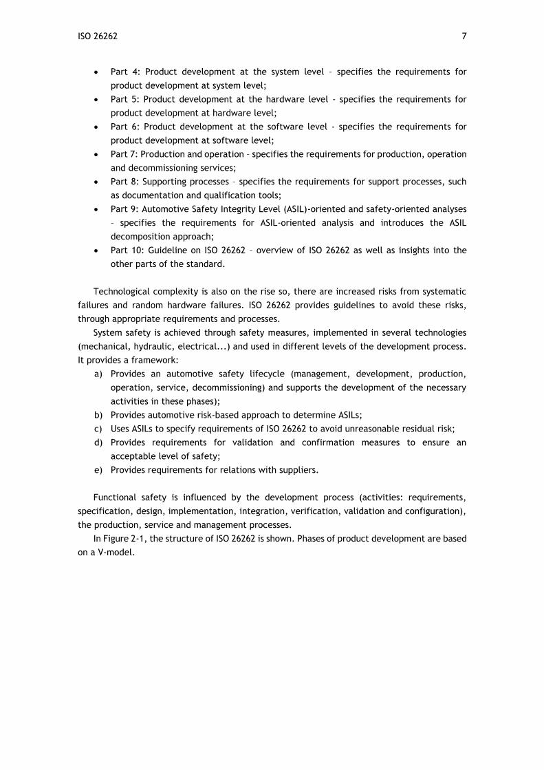
In Figure 2-1, the structure of ISO 26262 is shown. Phases of product development are based
on a V-model.
8 ISO 26262
Figure 2-1: Overview of ISO 26262 [1]
2.2.2. ASILs
These are the integrity levels in ISO 26262, similar to SILs. There are 5 ASILs: QM (no
integrity requirements), A, B, C and D (the highest safety requirement).
ASILs are assigned to hazards that may contribute to the violation of the safety goals,
according to the following parameters:
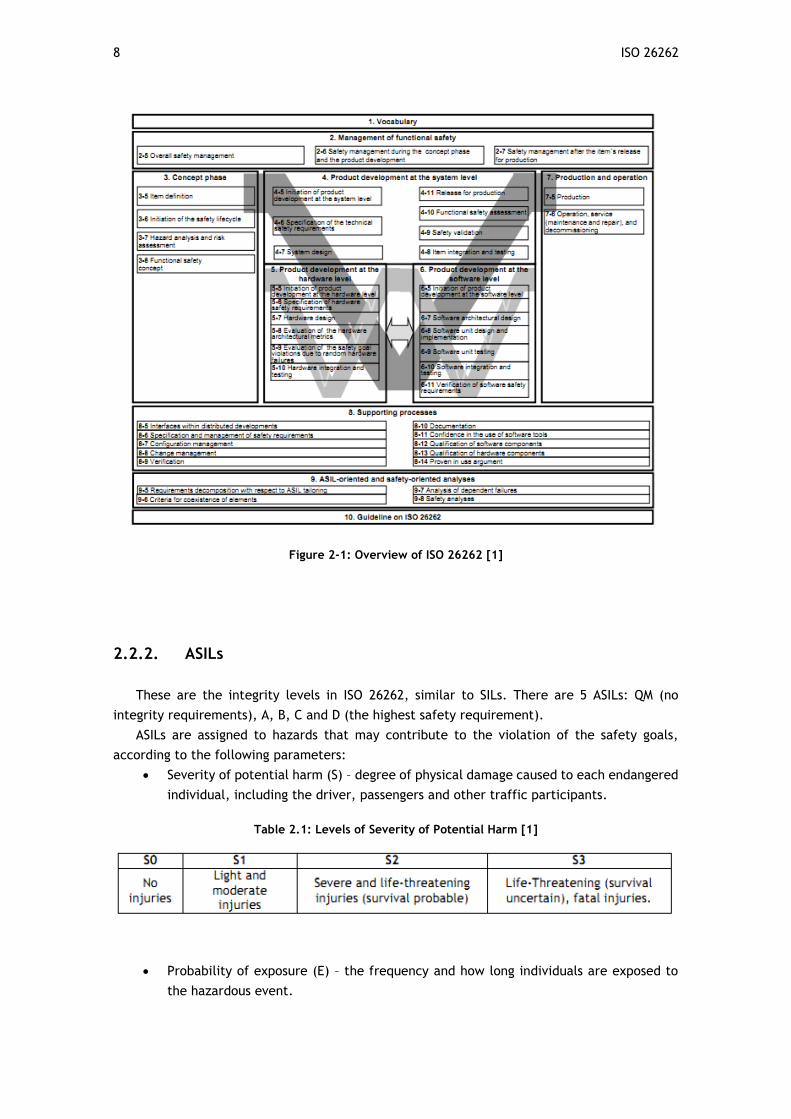
Severity of potential harm (S) – degree of physical damage caused to each endangered
individual, including the driver, passengers and other traffic participants.
Table 2.1: Levels of Severity of Potential Harm [1]
Probability of exposure (E) – the frequency and how long individuals are exposed to
the hazardous event.

Classic safety analysis techniques: FTA and FMEA 9
Table 2.2: Levels of Probability of Exposure [1]
Controllability (C) – the ability of the driver or other traffic participants
Table 2.3: Levels of controllability [1]
Then the assigned ASIL to each hazard is inferred with the rules presented in table 2.4.
Table 2.4: ASIL assignment, function of Severity, Exposure and Controllability [1]
These ASILs will be used to figure out the target values for the hardware evaluation metrics
that are going to be presented in chapter 3.
The events safety analysis have ASILs. The next section (2.3) introduces the two most
important safety analysis techniques.
2.3. Classic safety analysis techniques: FTA and FMEA
FTA (Fault Tree Analysis) is a top-down (deductive) graphical representation of logical
combinations of failures. It consists of a top event (system failure), connected to basic event(s)
using logical gates, like AND or OR. Basic events generally are component failures or events
expected to happen as normal operation of the system. The analysis is composed by two parts:
qualitative (logical) and quantitative (probabilistic) analysis. The objective of the first is to
reduce the logical expressions represented in the Fault Tree into a set of minimal cut sets,
which are the smallest combination of failures required to cause the top event. Quantitative
10 Modern Safety Analysis Tools and Techniques
analysis is used to calculate the probability of the top event, with the probability of each of
the basic events, this is only possible if the failure rate of the basic components is known [6].
FMEA is a bottom-up (inductive) technique, in which lists are compiled for all the possible
failure modes, using failures of the various parts of the system to infer the effects on the rest
of the system. These effects are usually evaluated according to a number of criteria, such as
severity, probability and detectability that are then combined into an overall estimate of risk.
All the information is combined in a table which allows to quickly see what the effects of each
failure mode are [6].
Both techniques are useful and provide important information about the systems, but both
suffer from the same flaw, they are manual techniques and the process to perform them can
be difficult and time-demanding, especially for large and complex systems. This makes the
whole process error prone or the results too numerous to interpret efficiently. Despite the
manual process being still predominant, there have been for some time now tools that support
the analysis, automating certain aspects of it [6].
2.4. Modern Safety Analysis Tools and Techniques
These appear as the need for automating parts or all the process of FTA and FMEA increases.
There are two categories for these tools. The first is compositional safety analysis approach
and consists in the development of formal and semi-formal languages to enable composition,
specification and analysis of system failure behavior, based on safety information about the
components. The majority of these tools are semi-automated, as they need manual entry of
the components failure information and can be useful in a model-based design process (e.g.:
HiP-HOPS). The second category involves more rigorous models to enable the analysis of the
effects of failures by simulating them and checking if the system meets the safety goals. To
achieve this, the tool adapts formal verification methods to support safety analysis [6].
2.4.1. Compositional Safety Analysis Techniques (CSA)
The first technique of this type is the Failure Propagation and Transformation Notation
(FPTN), a graphical description of the failure behavior of the system. This uses component
modules connected by inputs and outputs to other modules, allowing combination and
propagation of failures, also they can be decomposed by subsystems. Its purpose is to create a
connection between deductive FTA and inductive FMEA, in order to study cause and effect. The
inconvenience is the need to create an error model separate from the system model that can
become desynchronized from the original system. That being said, this technique is not used to
system analysis or design optimization, but only for describing specifications of failure.
Next comes Fault Propagation and Transformation Calculus (FPTC) that links the failure
model to the system model. It defines failure classes (e.g.: omission, commission and value
errors) that are specified in annotations in the components of the system model. Then failure
information is transmitted to the rest of the system by a set of expressions that detail how
failures are transformed and propagated from input to output (mitigation is possible by
transforming failure into natural behavior). This a “token-passing network”, determining the
effects of component failure in the entire system. It also allows quantitative analysis by
Automatic optimization of system reliability 11
including probabilities in the expressions. The advantage over FPTN is the use of system models,
so any small changes to it do not require a new failure model, but only the update of some
failure expressions. The disadvantage is that FPTC is inductive, because it relies on injecting
failures into the system, so it is difficult to achieve the information given by an FTA, also it is
prone to combinatorial explosion.
Other techniques based on FPTN are State-Event Fault Trees (SEFTs) and Component Fault
Trees (CFTs). The last technique is a failure logic of components defined graphically as
interconnected Fault Trees, the HiP-HOPS tool is similar to this approach. These are not
affected by combinatorial explosion as much as FPTC. SEFTs are based on CFTs and allow
analysis of dynamic systems as it distinguishes between a system in a state (over a period of
time) and an event that triggers a state transition (instantaneous). The failure behavior is
modelled at component level, but enables the representation of sequences and allows negation
(e.g.: event that has not happened yet) with the NOT gate. By being more complex, SEFTs can
be analyzed with FTA, so it uses a conversion to Deterministic Stochastic Petri Nets (DSPNs).
2.5. Automatic optimization of system reliability
As said before, manual safety analysis to evaluate different designs is highly time-consuming
and restricts the number of design candidates. This process needs to be automated, to examine
the most potential designs and choose the best suited for the objectives (cost, time, quality...).
Even with modern computers, it is not possible to evaluate the total design space, particularly
if multiple methods of variability are taken into account (e.g.: swapping a system architecture
for another and substituting one component with an alternative architecture). Another problem
is the main concern of system designers, cost. A balance between the two conflicting goals of
increasing reliability and cost reduction is required.
This section is just introductory, as HiP-HOPS allows the automatic optimization of system
designs. However, it will not be further developed, as it is not truly important to this thesis.
2.5.1. Different optimization approaches
The goal of the optimization is to find optimal solutions without the problem of getting
stuck in a local optimum. To reach this goal, there are different algorithms and almost all use
meta-heuristics.
One of this algorithms is tabu search, which is based on evaluation functions (e.g.: if a
solution has better characteristics, it is used for the next iteration), that can have multiple
objectives. This algorithm has memory, to prevent looping or getting stuck in a local optimum
(tabu solutions) [6].
Another technique is to use genetic algorithms. In this approach, a population of different
candidates is evaluated and the best individuals are chosen to reproduce and form the basis of
the next generation of candidates. Each one of these candidates has a genetic encoding, which
encloses its characteristics, then happens the crossover of the encodings. Random mutation
also happens to ensure a greater portion of search space and to avoid getting stuck in a local
optimum. There are different forms of genetic algorithms, including penalty-based approach,
in which the multiple objectives are combined into one function. One objective is optimized,
but the others are imposed constraints and if infringed, a penalty is subtracted from the fitness
score of the candidate. Another approach of genetic algorithms is the Non-Dominated Sorting
12 HiP-HOPS and Safety Analysis
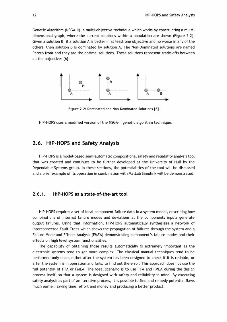
Genetic Algorithm (NSGA-II), a multi-objective technique which works by constructing a multi-
dimensional graph, where the current solutions within a population are shown (Figure 2-2).
Given a solution B, if a solution A is better in at least one objective and no worse in any of the
others, then solution B is dominated by solution A. The Non-Dominated solutions are named
Pareto front and they are the optimal solutions. These solutions represent trade-offs between
all the objectives [6].
Figure 2-2: Dominated and Non-Dominated Solutions [6]
HiP-HOPS uses a modified version of the NSGA-II genetic algorithm technique.
2.6. HiP-HOPS and Safety Analysis
HiP-HOPS is a model-based semi-automatic compositional safety and reliability analysis tool
that was created and continues to be further developed at the University of Hull by the
Dependable Systems group. In these sections, the potentialities of the tool will be discussed
and a brief example of its operation in combination with MatLab Simulink will be demonstrated.
2.6.1. HiP-HOPS as a state-of-the-art tool
HiP-HOPS requires a set of local component failure data in a system model, describing how
combinations of internal failure modes and deviations at the components inputs generate
output failures. Using that information, HiP-HOPS automatically synthesizes a network of
interconnected Fault Trees which shows the propagation of failures through the system and a
Failure Mode and Effects Analysis (FMEA) demonstrating component’s failure modes and their
effects on high level system functionalities.
The capability of obtaining those results automatically is extremely important as the
electronic systems tend to get more complex. The classical manual techniques tend to be
performed only once, either after the system has been designed to check if it is reliable, or
after the system is in operation and fails, to find out the error. This approach does not use the
full potential of FTA or FMEA. The ideal scenario is to use FTA and FMEA during the design
process itself, so that a system is designed with safety and reliability in mind. By executing
safety analysis as part of an iterative process, it is possible to find and remedy potential flaws
much earlier, saving time, effort and money and producing a better product.
HiP-HOPS and Safety Analysis 13
HiP-HOPS can be used as soon as a system’s concept can be turned into a model that
identifies components and material, energy or data transactions amongst them. Models can be
arranged hierarchically to deal with complexity. The tool can be used to analyse a variety of
systems, such as fluidic, electrical, electronic or mechanical [3].
Other capabilities of HiP-HOPS that contribute to the field of dependability include:
Temporal Fault Trees Generation:
It has become apparent that standard FTA and FMEA are poorly suited to analyse systems
in which time plays an important role [11]. Those systems may have multiple states of
operation, or a specific sequence of events may need to occur to originate a fault. To analyse
the failure behaviour of those systems, multiple fault trees are usually created to account for
each of the system’s states. Another solution is to enclose the temporal constraints within
event description. The two solutions can be unsatisfactory; the first can lead to complex and
fragmented analysis and the second can hide important temporal relations [11]. To overcome
the limitations of fault trees and FMEA concerning the referred systems, HiP-HOPS assesses
sequences of failures via synthesis of temporal fault trees and FMEAs. This technique is a result
of the integration of HiP-HOPS and Pandora. The latter is a method that enables modelling and
analysis of dynamic failure behaviour systems via extensions to Boolean Logic [11].
Multi-Objective optimization:
When there are various alternatives for a system’s architecture, they must be assessed in
accordance with the specific developer’s interests. This is a difficult, multi-objective problem
that can only be undertaken with the aid of computerized algorithms that allow effectively
optimal solutions to be found in large design spaces [3]. HiP-HOPS is capable of evaluating a
set of possible design alternatives according to user defined parameters such as cost and
dependability. The assessment of the different solutions is performed using a multi-objective
genetic algorithm that exploits the automated fault tree and FMEA synthesis algorithms in order
to find Pareto optimal architectures. These represent the optimal trade-offs between the
objective parameters considered by the system’s designer [3].
HiP-HOPS has the capability to consider preventive maintenance to evaluate dependability
and availability and through it, using also a genetic algorithm, the tool is capable of performing
multi-objective optimization of preventive maintenance schedules [5].
Linguistic concepts for representation and reuse of component failure patterns:
Well-established failure data can be stored in a library and reused posteriorly. This process
saves time and effort and it can be seen as a means for analysts who are unfamiliar with a
system to access viable information. Recurring patterns, like fail-silent behavior components,
for example, are the most promising elements of this technique [9]. The limitation faced by
the failure behavior reuse is the lack of a robust and machine-readable method to specify
failure data [9]. HiP-HOPS has the capability to solve this problem using Generalized Failure
Logic (GFL). Through a combination of Boolean Logic and generalized references to component
14 HiP-HOPS and Safety Analysis
ports and failure classes, GFL allows writing expressions that are applicable to multiple
components with the same failure behavior, even if their interfaces differ [9].
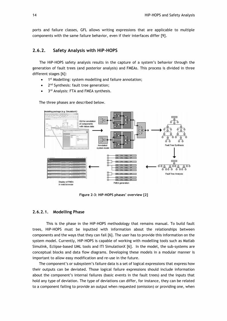
2.6.2. Safety Analysis with HiP-HOPS
The HiP-HOPS safety analysis results in the capture of a system’s behavior through the
generation of fault trees (and posterior analysis) and FMEAs. This process is divided in three
different stages [6]:
1st Modelling: system modelling and failure annotation;
2nd Synthesis: fault tree generation;
3rd Analysis: FTA and FMEA synthesis.
The three phases are described below.
Figure 2-3: HiP-HOPS phases’ overview [2]
2.6.2.1. Modelling Phase
This is the phase in the HiP-HOPS methodology that remains manual. To build fault
trees, HiP-HOPS must be inputted with information about the relationships between
components and the ways that they can fail [6]. The user has to provide this information on the
system model. Currently, HiP-HOPS is capable of working with modelling tools such as Matlab
Simulink, Eclipse-based UML tools and ITI SimulationX [6]. In the model, the sub-systems are
conceptual blocks and data flow diagrams. Developing these models in a modular manner is
important to allow easy modification and re-use in the future.
The component’s or subsystem’s failure data is a set of logical expressions that express how
their outputs can be deviated. Those logical failure expressions should include information
about the component’s internal failures (basic events in the fault trees) and the inputs that
hold any type of deviation. The type of deviations can differ, for instance, they can be related
to a component failing to provide an output when requested (omission) or providing one, when
HiP-HOPS and Safety Analysis 15
it was not requested (commission); deviations of value also exist, with either outputs with a
different value (higher or lower) than the correct one or temporarily incorrect (late or early).
As said before, the set of logical expressions used to illustrate the component’s failure
behavior, can be stored and re-used. A generalized example of a component’s commission
deviated output is presented below:
𝐶𝑜𝑚𝑚𝑖𝑠𝑠𝑖𝑜𝑛 − 𝑂𝑢𝑡1 = (𝐶𝑜𝑚𝑚𝑖𝑠𝑠𝑖𝑜𝑛 − 𝐼𝑛1 𝐴𝑁𝐷 𝐶𝑜𝑚𝑚𝑖𝑠𝑠𝑖𝑜𝑛 − 𝐼𝑛2)𝑂𝑅 𝐼𝑛𝑡𝑒𝑟𝑛𝑎𝑙𝐹𝑎𝑖𝑙𝑢𝑟𝑒1
The Commission of output1 (Out1) is caused either by the combination of the Commission
of input1 and input2 or by an internal failure of the component.
Generalizing the HiP-HOPS terminology rules:
Inputs and outputs: “type of deviation” – “name of the I/O in the model”;
Internal failures can assume the form of valid identifiers. For example: “short circuit”.
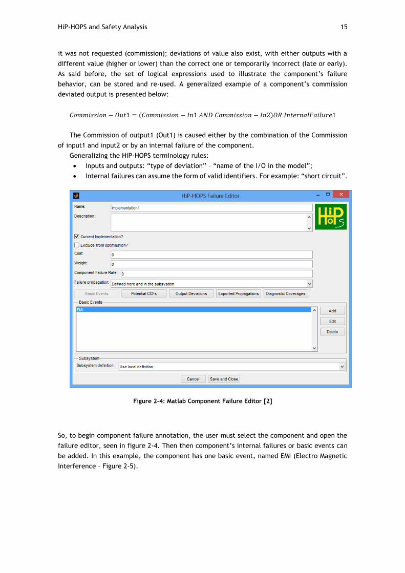
Figure 2-4: Matlab Component Failure Editor [2]
So, to begin component failure annotation, the user must select the component and open the
failure editor, seen in figure 2-4. Then then component’s internal failures or basic events can
be added. In this example, the component has one basic event, named EMI (Electro Magnetic
Interference – Figure 2-5).
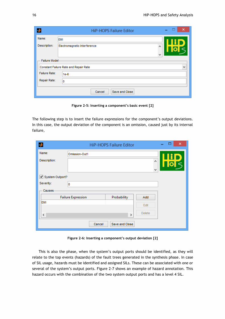
16 HiP-HOPS and Safety Analysis
Figure 2-5: Inserting a component’s basic event [2]
The following step is to insert the failure expressions for the component’s output deviations.
In this case, the output deviation of the component is an omission, caused just by its internal
failure,
Figure 2-6: Inserting a component’s output deviation [2]
This is also the phase, when the system’s output ports should be identified, as they will
relate to the top events (hazards) of the fault trees generated in the synthesis phase. In case
of SIL usage, hazards must be identified and assigned SILs. These can be associated with one or
several of the system’s output ports. Figure 2-7 shows an example of hazard annotation. This
hazard occurs with the combination of the two system output ports and has a level 4 SIL.
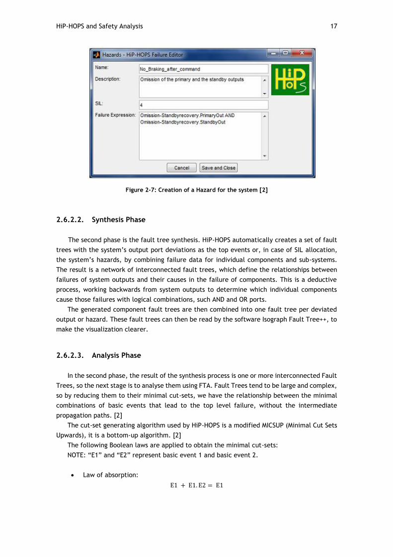
HiP-HOPS and Safety Analysis 17
Figure 2-7: Creation of a Hazard for the system [2]
2.6.2.2. Synthesis Phase
The second phase is the fault tree synthesis. HiP-HOPS automatically creates a set of fault
trees with the system’s output port deviations as the top events or, in case of SIL allocation,
the system’s hazards, by combining failure data for individual components and sub-systems.
The result is a network of interconnected fault trees, which define the relationships between
failures of system outputs and their causes in the failure of components. This is a deductive
process, working backwards from system outputs to determine which individual components
cause those failures with logical combinations, such AND and OR ports.
The generated component fault trees are then combined into one fault tree per deviated
output or hazard. These fault trees can then be read by the software Isograph Fault Tree++, to
make the visualization clearer.
2.6.2.3. Analysis Phase
In the second phase, the result of the synthesis process is one or more interconnected Fault
Trees, so the next stage is to analyse them using FTA. Fault Trees tend to be large and complex,
so by reducing them to their minimal cut-sets, we have the relationship between the minimal
combinations of basic events that lead to the top level failure, without the intermediate
propagation paths. [2]
The cut-set generating algorithm used by HiP-HOPS is a modified MICSUP (Minimal Cut Sets
Upwards), it is a bottom-up algorithm. [2]
The following Boolean laws are applied to obtain the minimal cut-sets:
NOTE: “E1” and “E2” represent basic event 1 and basic event 2.
Law of absorption:
E1 + E1. E2 = E1
18 HiP-HOPS and Safety Analysis
The cut set “E1.E2” was removed as the event “E1” alone is sufficient to cause the
top event. [2]
Laws of idempotence:
E1. E1 = E1
Repeated events in the same cut-set are removed [2].
𝐸1 + 𝐸1 = 𝐸1
Repeated cut-sets are removed [2].
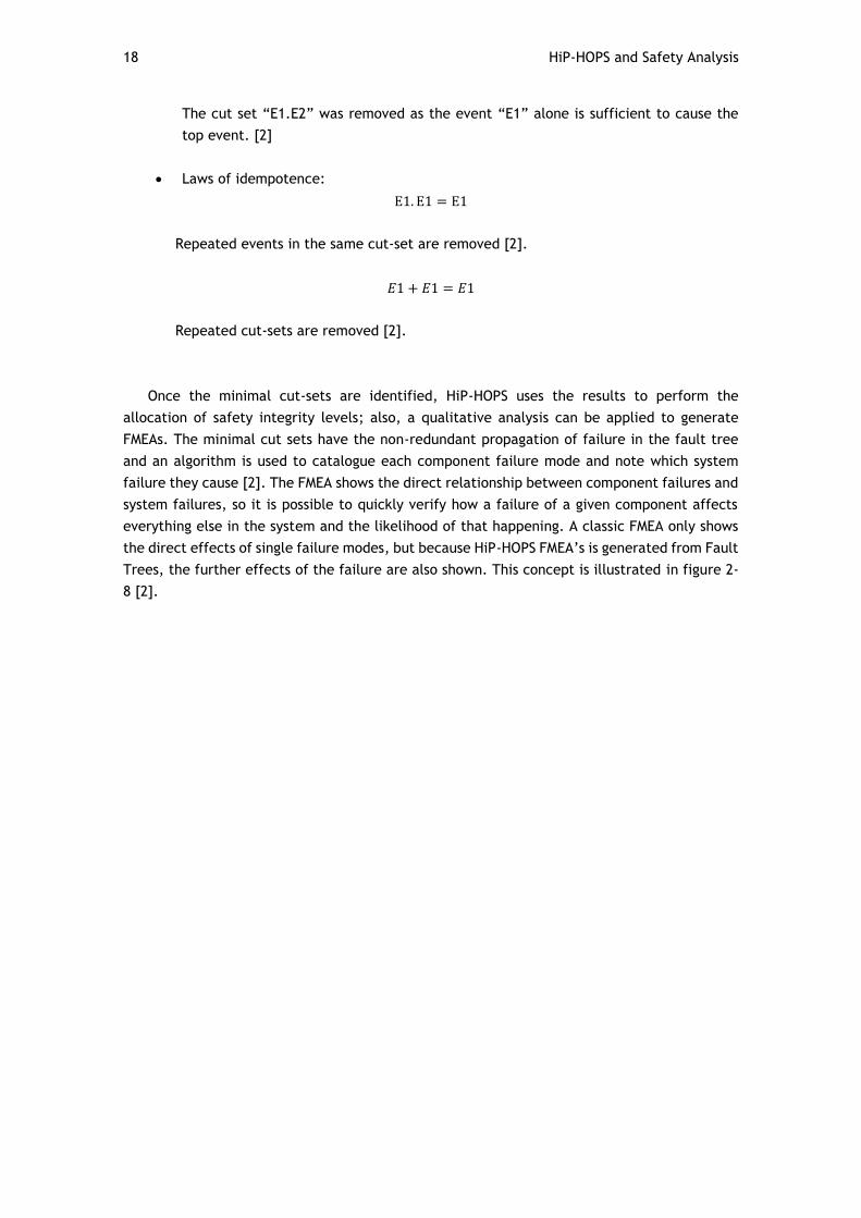
Once the minimal cut-sets are identified, HiP-HOPS uses the results to perform the
allocation of safety integrity levels; also, a qualitative analysis can be applied to generate
FMEAs. The minimal cut sets have the non-redundant propagation of failure in the fault tree
and an algorithm is used to catalogue each component failure mode and note which system
failure they cause [2]. The FMEA shows the direct relationship between component failures and
system failures, so it is possible to quickly verify how a failure of a given component affects
everything else in the system and the likelihood of that happening. A classic FMEA only shows
the direct effects of single failure modes, but because HiP-HOPS FMEA’s is generated from Fault
Trees, the further effects of the failure are also shown. This concept is illustrated in figure 2-
8 [2].
HiP-HOPS and Safety Analysis 19
Figure 2-8: Conversion of Fault Trees to FMEA [2]
In Figure 2-8, “F1” and “F2” are system Failures and “C1” to “C9” are component Failures.
For “C3”, “C4”, “C6” and “C7” there are no direct effects on the system, but only if a single
one of this components fails, if, for example, “C3” and “C4” both happen, “F1” will occur.
A quantitative analysis can also be done, to calculate the system unavailability, QS (if basic
events have quantitative data [2]):
Q𝑆 = 1 − ∏(1 − 𝑄𝐶𝑆𝑖)
𝑛
𝑖 =1
𝑛 − 𝑛𝑢𝑚𝑏𝑒𝑟 𝑜𝑓 𝑖𝑛𝑑𝑒𝑝𝑒𝑛𝑑𝑒𝑛𝑡 𝑐𝑢𝑡 𝑠𝑒𝑡𝑠
𝑄𝐶𝑆𝑖 − 𝑢𝑛𝑎𝑣𝑎𝑖𝑙𝑎𝑏𝑖𝑙𝑖𝑡𝑦 𝑜𝑓 𝑡ℎ𝑒 𝑐𝑢𝑡 𝑠𝑒𝑡 𝑖
The resultant fault trees, cut sets, FMEAs and SIL allocations are presented in html format.
Currently, the files generated can only be opened with Internet Explorer [16].
20 HiP-HOPS and Safety Analysis
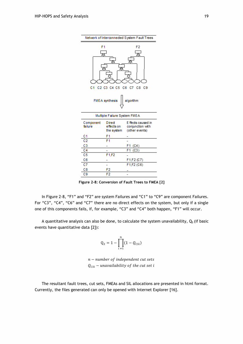
Figure 2-9: Fault tree analysis summary [2]
Each fault tree has a name, which is constructed from the name of the output deviation
they come from. Clicking on a fault tree name opens that fault tree results (figure 2-10) [2].
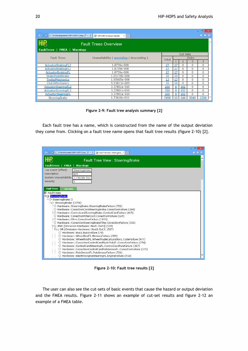
Figure 2-10: Fault tree results [2]
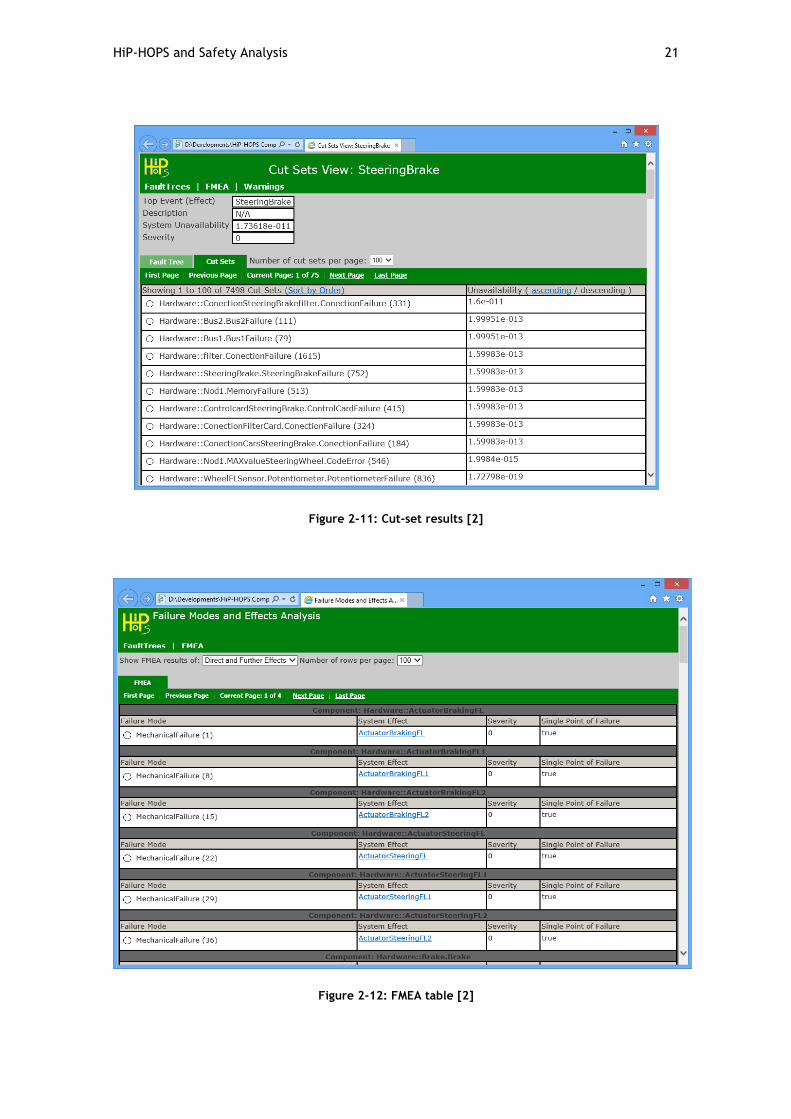
The user can also see the cut-sets of basic events that cause the hazard or output deviation
and the FMEA results. Figure 2-11 shows an example of cut-set results and figure 2-12 an
example of a FMEA table.
HiP-HOPS and Safety Analysis 21
Figure 2-11: Cut-set results [2]
Figure 2-12: FMEA table [2]
22 Summary
2.7. Summary
In this chapter it became clear that safety analysis plays a major role in hardware
development, and that with the increasing complexity of E/E/EP systems, automatic safety
analysis tools like HiP-HOPS are increasingly important to produce more reliable products. It
was also evident how easy it is to use HiP-HOPS.
HiP-HOPS lacks some of the ideas and rules in ISO 26262, for hardware architecture
evaluation. The next chapter will be an in-depth analysis of ISO 26262 – part 5, particularly,
how are safety mechanisms modelled according to the standard and how to use the hardware
verification metrics present there.
3.1. Introduction 23
Chapter 3
Hardware evaluation techniques
This chapter is a full analysis of ISO 26262 – part 5: product development at hardware level.
The intention is to understand how safety mechanisms should be modelled according to the
standard and what hardware evaluation metrics are. Then, changes to HiP-HOPS will be
proposed, to accommodate these concepts.
3.1. Introduction
This part of the standard specifies requirements for product development at hardware level
for automotive applications, such as [1]:
Requirements for the initiation of product development;
Specification of the hardware safety requirements;
Hardware design;
Hardware architectural metrics;
Evaluation of violation of the safety goal due to random hardware failures.
This requirements are applicable to non-programmable and programmable elements, like
FPGA and PLD [1].
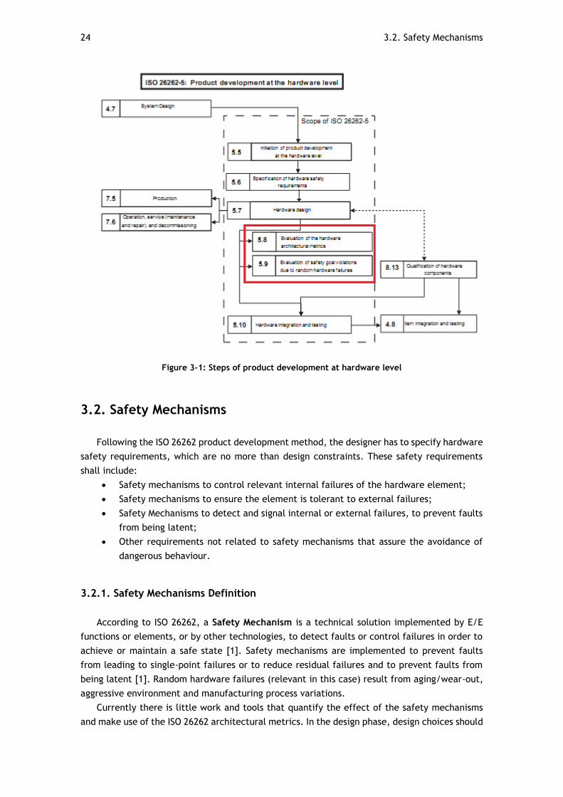
The steps required for the product development process, according to ISO 26262, are
resumed in figure 3-1. The phases, especially explored in this thesis, are highlighted,
“evaluation of the hardware architectural metrics” and “evaluation of safety goal violations
due to random hardware failures”. There are two sections dedicated to those phases, sections
8 and 9 in ISO 26262 – part 5, which describe two alternatives to evaluate if the residual risk of
safety goal violations is sufficiently low. They accomplish this by either using a global
probabilistic approach or by using a cut-set analysis to study the impact of each identified fault
of a hardware element upon the violation of the safety goals [1].
24 3.2. Safety Mechanisms
Figure 3-1: Steps of product development at hardware level
3.2. Safety Mechanisms
Following the ISO 26262 product development method, the designer has to specify hardware
safety requirements, which are no more than design constraints. These safety requirements
shall include:
Safety mechanisms to control relevant internal failures of the hardware element;
Safety mechanisms to ensure the element is tolerant to external failures;
Safety Mechanisms to detect and signal internal or external failures, to prevent faults
from being latent;
Other requirements not related to safety mechanisms that assure the avoidance of
dangerous behaviour.
3.2.1. Safety Mechanisms Definition
According to ISO 26262, a Safety Mechanism is a technical solution implemented by E/E
functions or elements, or by other technologies, to detect faults or control failures in order to
achieve or maintain a safe state [1]. Safety mechanisms are implemented to prevent faults
from leading to single-point failures or to reduce residual failures and to prevent faults from
being latent [1]. Random hardware failures (relevant in this case) result from aging/wear-out,
aggressive environment and manufacturing process variations.
Currently there is little work and tools that quantify the effect of the safety mechanisms
and make use of the ISO 26262 architectural metrics. In the design phase, design choices should
3.2. Safety Mechanisms 25
be compared with the safety mechanisms included, as these contribute to the final failure rate
of the system. In ISO 26262-part 5, safety mechanisms are recommended to certain component
faults.
Other important concepts, related to Safety Mechanisms are presented below:
Diagnostic Coverage: “proportion of the hardware element failure rate that is
detected or controlled by the implemented safety mechanisms [1]”;
3.2.2. Choice of Safety Mechanisms
ISO 26262 offers a guideline to choose appropriate safety mechanisms to be implemented
in the E/E architecture to detect failures of elements [1].
The Annex D, in ISO 26262 part 5 is intended to be used as [1]:
a) An evaluation of the Diagnostic Coverage to produce a rationale for:
1) The compliance with the single-point and latent faults metrics;
2) The compliance with the evaluation of the safety goal violations due to random
hardware failures:
b) A guideline in order to choose appropriate safety mechanisms to be implemented in
the E/E architecture to detect failures of elements. [1]
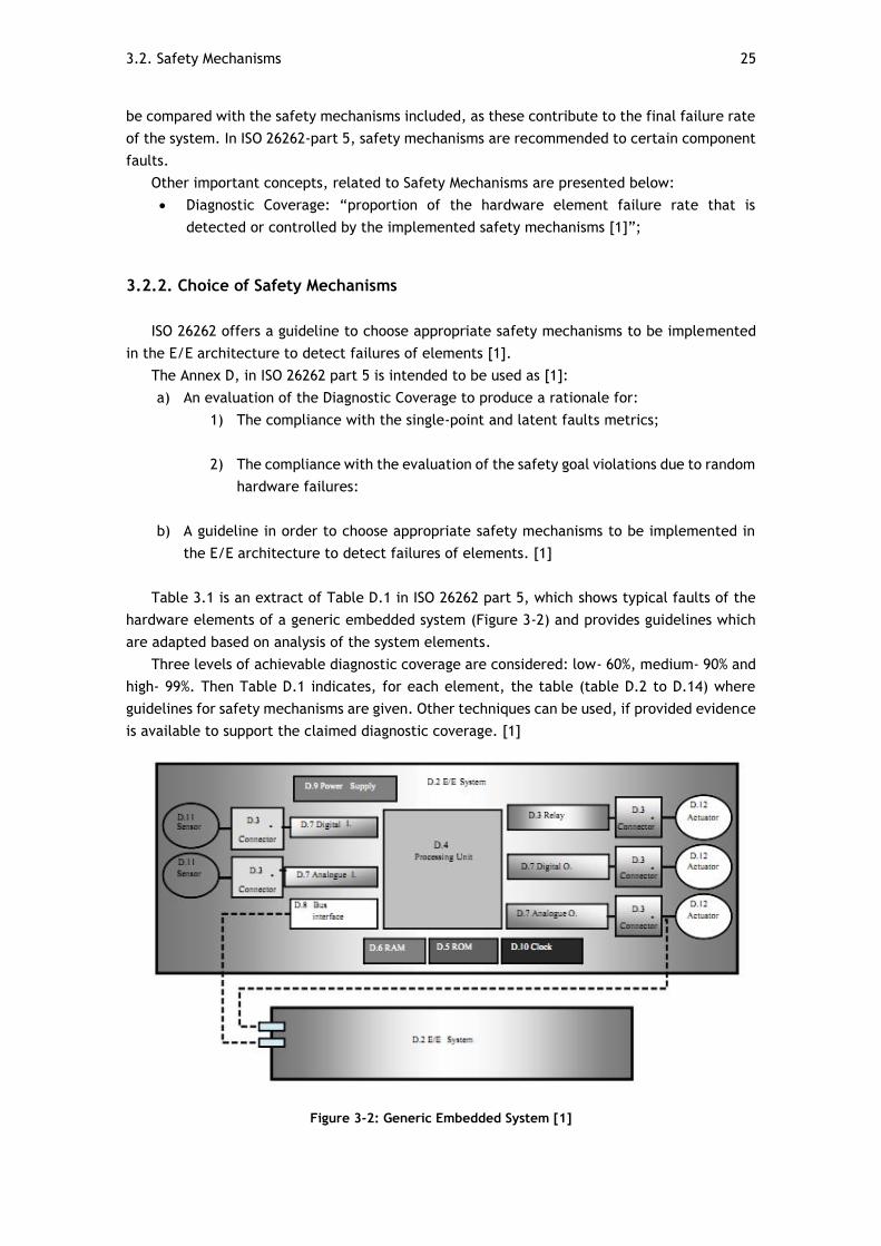
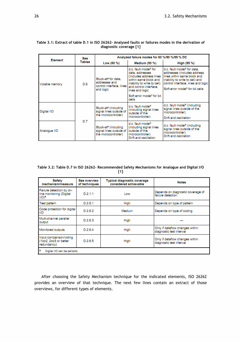
Table 3.1 is an extract of Table D.1 in ISO 26262 part 5, which shows typical faults of the
hardware elements of a generic embedded system (Figure 3-2) and provides guidelines which
are adapted based on analysis of the system elements.
Three levels of achievable diagnostic coverage are considered: low- 60%, medium- 90% and
high- 99%. Then Table D.1 indicates, for each element, the table (table D.2 to D.14) where
guidelines for safety mechanisms are given. Other techniques can be used, if provided evidence
is available to support the claimed diagnostic coverage. [1]
Figure 3-2: Generic Embedded System [1]
26 3.2. Safety Mechanisms
Table 3.1: Extract of table D.1 in ISO 26262- Analysed faults or failures modes in the derivation of
diagnostic coverage [1]
Table 3.2: Table D.7 in ISO 26262– Recommended Safety Mechanisms for Analogue and Digital I/O
[1]
After choosing the Safety Mechanism technique for the indicated elements, ISO 26262
provides an overview of that technique. The next few lines contain an extract of those
overviews, for different types of elements.
3.2. Safety Mechanisms 27
For electrical elements, such as relays or sensors, the common safety mechanism selected
for this study is the Comparator [1]:
Aim: To detect (non-simultaneous) failures in independent hardware or software.
Description: The output signals of independent hardware are compared cyclically or
continuously by a comparator. For example, two processing units exchange data
reciprocally. A comparison is carried out using software in each unit and detected
differences lead to a failure message.
Processing Units are some of the most complex elements in a hardware architecture, they
can have hardware or software safety mechanisms, sometimes even both. I have selected the
self-test supported by hardware [1]:
Description: additional special hardware to support self-test functions to detect
failures in the processing unit and other sub-elements (e.g.: EDC coder/decoder) at a
gate level. Typically it only runs at the initialization or power-down of the processing
unit due to its intrusive nature. It is usually used for multipoint fault detection.
Example: For sub-elements like EDC coders/decoders, a special HW mechanism (e.g.:
logic BIST) can be added to generate inputs to the coder-decoder and check the
results. These inputs are usually generated by pattern generators (e.g. MISR).
NOTE: Logic BIST - Logic built-in self-test (or LBIST) is a form of built-in self-test (BIST) in
which hardware and/or software is built into integrated circuits allowing them to test their
own operation, as opposed to reliance on external automated test equipment.
For actuators, the example is a technique named Monitoring [1]:
Aim: detect incorrect operation of an actuator
Description: The operation of the actuator is monitored. Can be done at the actuator
level by physical parameter measurements but also at system level regarding the
actuator failure effect.
Example: A cooling fan, monitoring at system level uses a temperature sensor to
detect failure. Monitoring of physical parameters measures the voltage, current or
both on the inputs of the cooling fan.
3.2.3. How to Model Safety Mechanisms
In the sections above, safety mechanisms were introduced and examples of guidelines to
properly select them according to the E/E element in cause were given. The remaining issue is
how a designer can model a safety mechanism in a system model.
ISO 26262 - part 5, annex E is an example of metrics calculation. That example can help
understand, along with other parts of the standard, the constraints of safety mechanism design.
The following conclusions were reached concerning safety mechanism insertion in system’s
models:
One Safety Mechanism can cover several failure modes of different components,
considered in the safety analysis for the same safety goal.

28 3.2. Safety Mechanisms
This point is evident in Table 3.3. SM2 (safety mechanism 2) is a comparator that compares
the values of two inputs. The components that are covered by that safety mechanism influence,
somehow, the values checked by it;
Table 3.3: Extract of Figure E.3 in ISO 26262 – part 5, annex E
Safety Mechanisms should have a flexible description, regarding its particular
attributes, as they can assume different forms (software, hardware, different
algorithms…) [10];
The applicability of specific safety mechanisms to a certain component has to be
resolved by component class hierarchy [10];
Architectural evolution must be considered by safety mechanisms [10];
A safety mechanism can be a component or a part of a component. For example, a
microcontroller can have self-check hardware in its architecture or an external
watchdog.
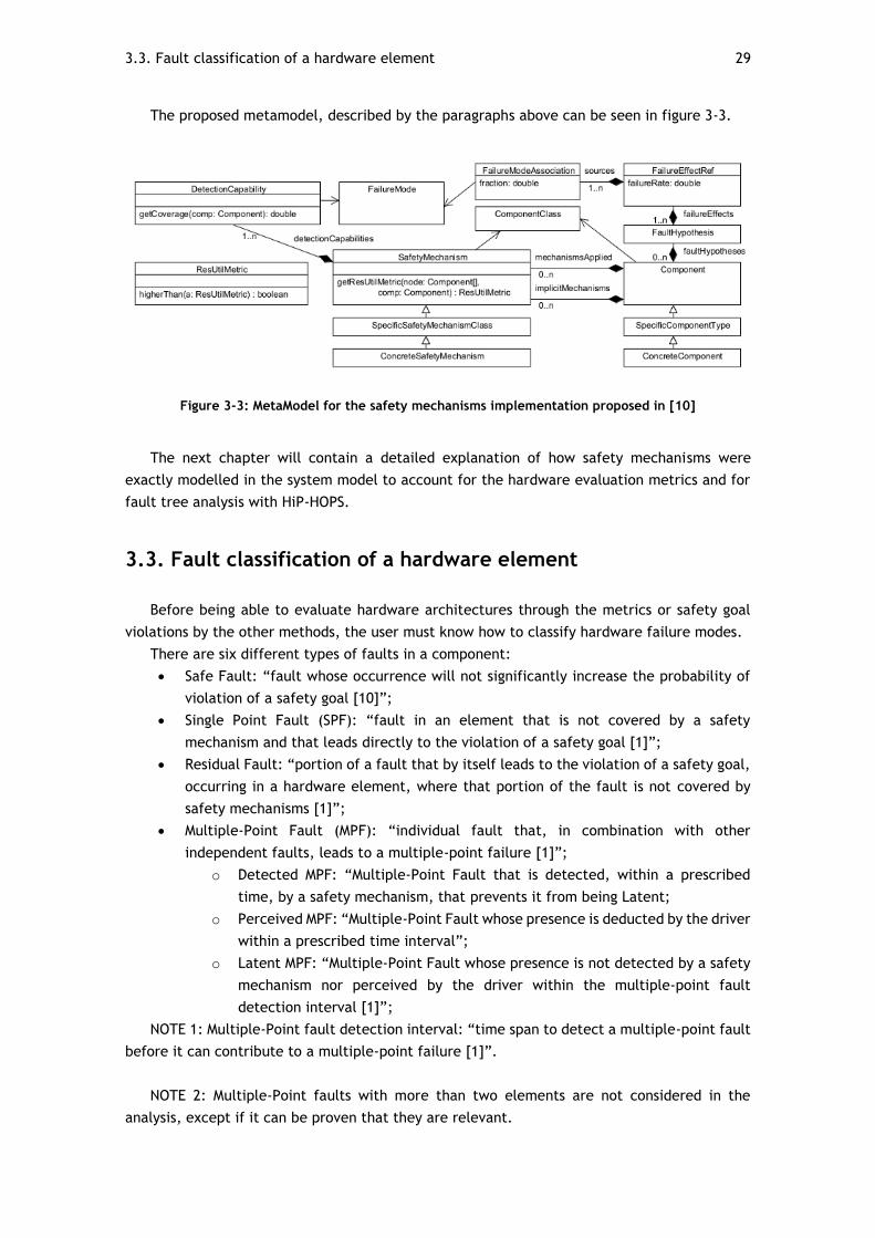
In [10] the authors propose an interesting way to model safety mechanisms. They consider
a model represented by a set of computing nodes, where functional networks are responsible
for the execution of each item and network or bus connections between those [10]. A node is
modelled by a list of component and a list of safety mechanism instances [{Cj}, {SMk}]. A
component Ci is a source of a set of failure effects {FECj,k} that can lead to the violation of the
safety goal on the top level. These failure effects are included into the Component’s
faultHypotesis. A failure effect FE can be caused by a number of different failure modes {FMi},
which are associated by FaultHypothesis with a fraction KFMi,Cj as percentage of the failure rate
for an effect caused by a specific failure mode [10].
A safety mechanism is modelled as possessing one or more detection capabilities. An object
of the class DetectionCapability characterizes mechanism’s coverage DC of specific failure
modes, of specific component classes CC, that can be represented by [{CCi, FMi, DCi}]. When
a safety mechanism is instantiated in a model, it is applied to one or more components by
adding it to the mechanismsApplied reference list, or to the implicitMechanisms reference list,
if the SM is implicit to that component [10].
3.3. Fault classification of a hardware element 29
The proposed metamodel, described by the paragraphs above can be seen in figure 3-3.
Figure 3-3: MetaModel for the safety mechanisms implementation proposed in [10]
The next chapter will contain a detailed explanation of how safety mechanisms were
exactly modelled in the system model to account for the hardware evaluation metrics and for
fault tree analysis with HiP-HOPS.
3.3. Fault classification of a hardware element
Before being able to evaluate hardware architectures through the metrics or safety goal
violations by the other methods, the user must know how to classify hardware failure modes.
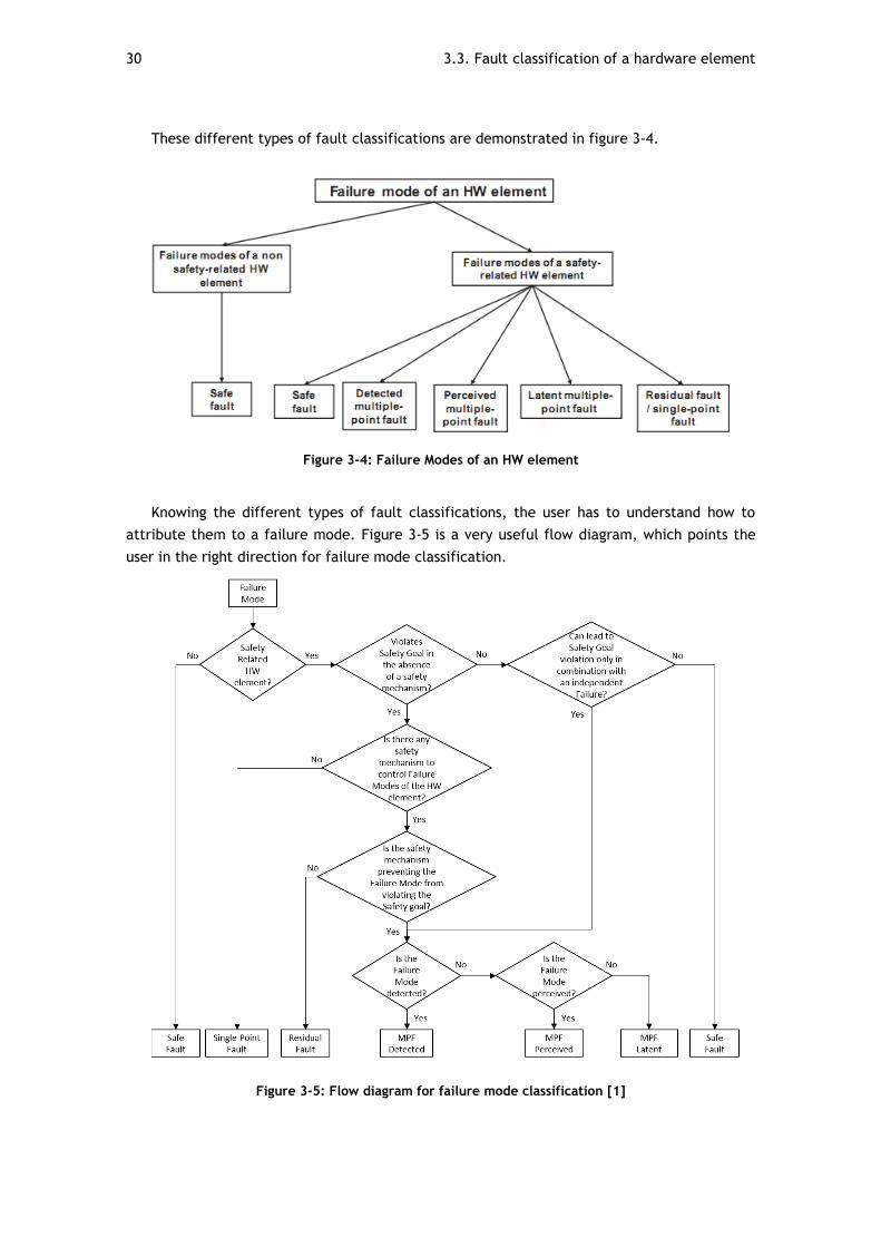
There are six different types of faults in a component:
Safe Fault: “fault whose occurrence will not significantly increase the probability of
violation of a safety goal [10]”;
Single Point Fault (SPF): “fault in an element that is not covered by a safety
mechanism and that leads directly to the violation of a safety goal [1]”;
Residual Fault: “portion of a fault that by itself leads to the violation of a safety goal,
occurring in a hardware element, where that portion of the fault is not covered by
safety mechanisms [1]”;
Multiple-Point Fault (MPF): “individual fault that, in combination with other
independent faults, leads to a multiple-point failure [1]”;
o Detected MPF: “Multiple-Point Fault that is detected, within a prescribed
time, by a safety mechanism, that prevents it from being Latent;
o Perceived MPF: “Multiple-Point Fault whose presence is deducted by the driver
within a prescribed time interval”;
o Latent MPF: “Multiple-Point Fault whose presence is not detected by a safety
mechanism nor perceived by the driver within the multiple-point fault
detection interval [1]”;
NOTE 1: Multiple-Point fault detection interval: “time span to detect a multiple-point fault
before it can contribute to a multiple-point failure [1]”.
NOTE 2: Multiple-Point faults with more than two elements are not considered in the
analysis, except if it can be proven that they are relevant.
30 3.3. Fault classification of a hardware element
These different types of fault classifications are demonstrated in figure 3-4.
Figure 3-4: Failure Modes of an HW element
Knowing the different types of fault classifications, the user has to understand how to
attribute them to a failure mode. Figure 3-5 is a very useful flow diagram, which points the
user in the right direction for failure mode classification.
Figure 3-5: Flow diagram for failure mode classification [1]
3.4. ISO 26262 Hardware Metrics 31
3.4. ISO 26262 Hardware Metrics
As it has been said before, the 5th part of the ISO 26262 presents two metrics to evaluate
the effectiveness of hardware architectures to cope with random hardware failures [1]. The
results are then compared to target values, if those targets are not achieved, then the
architecture must be improved by changing components or safety mechanisms. The hardware
architectural metrics can be applied iteratively during the design phase and are dependent on
the whole hardware of the item. [1]
There are also two other evaluations, that check the safety goal violations due to random
hardware failures [1]. These are complementary to the metrics and are also going to be
described.
To proceed with the metric evaluation, the designer has to estimate the failure rate of the
components in the architecture that are relevant to the analysis. The estimated failure rate for
the hardware parts of the item shall be determined:
a) Using hardware failure rate data from a recognized industry source (e.g.: IEC/TR 62380,
IEC 61709, MIL HDBK 217 F notice 2,…), or [1]
b) Using statistics based on field tests. The estimated failure rate should have an adequate
confidence level, or [1]
c) Using expert judgment founded on an engineering approach based on quantitative or
qualitative arguments. A structured criteria should be the base for this judgment [1]
3.4.1 Architectural Metrics
There are two metrics described in ISO 26262, Single-Point Fault Metric and Latent Fault
Metric. These evaluate the system’s robustness, through the coverage from safety mechanisms.
Higher metric values reflect safer systems, therefore low percentage of critical faults (single-
point faults and residual/latent faults).
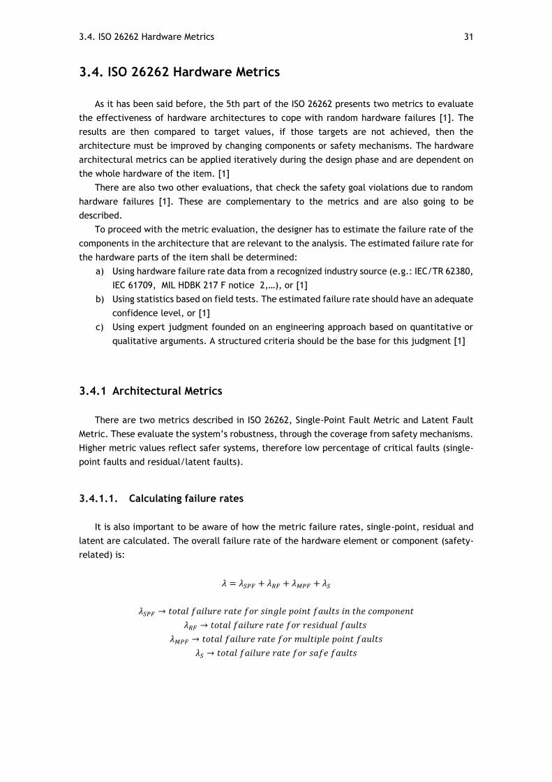
3.4.1.1. Calculating failure rates
It is also important to be aware of how the metric failure rates, single-point, residual and
latent are calculated. The overall failure rate of the hardware element or component (safety-
related) is:
𝜆 = 𝜆𝑆𝑃𝐹 + 𝜆𝑅𝐹 + 𝜆𝑀𝑃𝐹 + 𝜆𝑆
𝜆𝑆𝑃𝐹 → 𝑡𝑜𝑡𝑎𝑙 𝑓𝑎𝑖𝑙𝑢𝑟𝑒 𝑟𝑎𝑡𝑒 𝑓𝑜𝑟 𝑠𝑖𝑛𝑔𝑙𝑒 𝑝𝑜𝑖𝑛𝑡 𝑓𝑎𝑢𝑙𝑡𝑠 𝑖𝑛 𝑡ℎ𝑒 𝑐𝑜𝑚𝑝𝑜𝑛𝑒𝑛𝑡
𝜆𝑅𝐹 → 𝑡𝑜𝑡𝑎𝑙 𝑓𝑎𝑖𝑙𝑢𝑟𝑒 𝑟𝑎𝑡𝑒 𝑓𝑜𝑟 𝑟𝑒𝑠𝑖𝑑𝑢𝑎𝑙 𝑓𝑎𝑢𝑙𝑡𝑠
𝜆𝑀𝑃𝐹 → 𝑡𝑜𝑡𝑎𝑙 𝑓𝑎𝑖𝑙𝑢𝑟𝑒 𝑟𝑎𝑡𝑒 𝑓𝑜𝑟 𝑚𝑢𝑙𝑡𝑖𝑝𝑙𝑒 𝑝𝑜𝑖𝑛𝑡 𝑓𝑎𝑢𝑙𝑡𝑠
𝜆𝑆 → 𝑡𝑜𝑡𝑎𝑙 𝑓𝑎𝑖𝑙𝑢𝑟𝑒 𝑟𝑎𝑡𝑒 𝑓𝑜𝑟 𝑠𝑎𝑓𝑒 𝑓𝑎𝑢𝑙𝑡𝑠
32 3.4. ISO 26262 Hardware Metrics
Single-point faults are not covered by any safety mechanism, therefore, the failure rate for
single-point faults (𝜆𝑆𝑃𝐹) in the component is, simply, the failure rate of the fault (failure rate
of the component, multiplied by the failure mode distribution):
𝜆𝑆𝑃𝐹 = 𝜆
𝜆 → 𝑓𝑎𝑖𝑙𝑢𝑟𝑒 𝑟𝑎𝑡𝑒 𝑜𝑓 𝑡ℎ𝑒 𝑓𝑎𝑢𝑙𝑡
The residual fault’s failure rate (𝜆𝑅𝐹(𝑒𝑠𝑡)) is determined from the diagnostic coverage of the
safety mechanisms. A single-point fault can be prevented, mitigated or eliminated by a safety
mechanism and the hazard only happens if the mechanism fails. However, if the diagnostic
coverage in not 100%, the fault can be a residual fault, then the estimated failure rate is:
𝜆𝑅𝐹(𝑒𝑠𝑡) = 𝜆 × (1 − (𝐾𝐷𝐶−𝑅𝐹 100⁄ ))
𝐾𝐷𝐶−𝑅𝐹 → 𝑑𝑖𝑎𝑔𝑛𝑜𝑠𝑡𝑖𝑐 𝑐𝑜𝑣𝑒𝑟𝑎𝑔𝑒 𝑝𝑒𝑟𝑐𝑒𝑛𝑡𝑎𝑔𝑒 𝑖𝑛 𝑟𝑒𝑠𝑖𝑑𝑢𝑎𝑙 𝑓𝑎𝑢𝑙𝑡𝑠
𝜆 → 𝑓𝑎𝑖𝑙𝑢𝑟𝑒 𝑟𝑎𝑡𝑒 𝑜𝑓 𝑡ℎ𝑒 𝑓𝑎𝑢𝑙𝑡 𝑐𝑜𝑣𝑒𝑟𝑒𝑑 𝑏𝑦 𝑡ℎ𝑒 𝑠𝑎𝑓𝑒𝑡𝑦 𝑚𝑒𝑐ℎ𝑎𝑛𝑖𝑠𝑚
The faults that lead directly to the violation of the safety goal, single-point faults or residual
faults, cannot contribute anymore to the latent faults population [1].
MPF is the sum of perceived or detected multiple point faults and latent faults. This
breaking down introduces the concept of detectability using diagnostic coverage: some faults
are perceived by the driver directly and some are detected by safety mechanisms. Latent faults
are not detected.
Therefore, the failure rate of the latent failure mode (𝜆𝑀𝑃𝐹−𝐿(𝑒𝑠𝑡)) that is perceived by the
driver or covered by a safety mechanism is the remaining failure rate of the residual fault,
being covered by a safety mechanism, multiplied by the percentage of the estimated
unperceived faults by the driver or uncovered faults by the safety mechanism:
𝜆𝑀𝑃𝐹−𝐿(𝑒𝑠𝑡) = (𝜆 − 𝜆𝑅𝐹(𝑒𝑠𝑡)) × (1 − (𝐾𝐷𝐶−𝑀𝑃𝐹−𝐿 100⁄ ))
𝐾𝐷𝐶−𝑀𝑃𝐹−𝐿 → 𝑒𝑠𝑡𝑖𝑚𝑎𝑡𝑒𝑑 𝑝𝑒𝑟𝑐𝑒𝑛𝑡𝑎𝑔𝑒 𝑜𝑓 𝑐𝑜𝑣𝑒𝑟𝑒𝑑 𝑜𝑟 𝑝𝑒𝑟𝑐𝑒𝑖𝑣𝑒𝑑 𝑓𝑎𝑢𝑙𝑡𝑠
𝜆 → 𝑓𝑎𝑖𝑙𝑢𝑟𝑒 𝑟𝑎𝑡𝑒 𝑜𝑓 𝑡ℎ𝑒 𝑓𝑎𝑢𝑙𝑡 𝑐𝑜𝑣𝑒𝑟𝑒𝑑 𝑏𝑦 𝑡ℎ𝑒 𝑠𝑎𝑓𝑒𝑡𝑦 𝑚𝑒𝑐ℎ𝑎𝑛𝑖𝑠𝑚
𝜆𝑅𝐹(𝑒𝑠𝑡) → 𝑓𝑎𝑖𝑙𝑢𝑟𝑒 𝑟𝑎𝑡𝑒 𝑜𝑓 𝑡ℎ𝑒 𝑟𝑒𝑠𝑖𝑑𝑢𝑎𝑙 𝑓𝑎𝑢𝑙𝑡
However, a component can also be latent through degradation of its capabilities. The
component still works, but if certain external conditions like electromagnetic interference or
harsh atmospheric conditions occur, the component can fail. That is the combination of two
basic events, despite the difficulty of expressing the external condition’s failure rate, and
according to the flow diagram for failure mode classification (Figure 3-5), this is a latent
multiple-point failure. In ISO 26262 - part 5, annex E, examples of this type of MPFs are given.
For the calculations of the metric, they don’t consider the failure rate of the external event
that triggers the fault, therefore, the failure rate for this kind of multiple point faults is just
the failure rate of the failure mode:
𝜆𝑀𝑃𝐹−𝐿(𝑒𝑠𝑡) = 𝜆
3.4. ISO 26262 Hardware Metrics 33
𝜆 → 𝑓𝑎𝑖𝑙𝑢𝑟𝑒 𝑟𝑎𝑡𝑒 𝑜𝑓 𝑡ℎ𝑒 𝑓𝑎𝑢𝑙𝑡
3.4.1.2. Metrics
Now that the failure rates included in the hardware architectural metrics are explored, the
values for the two metrics, single-point and latent, can be demonstrated.
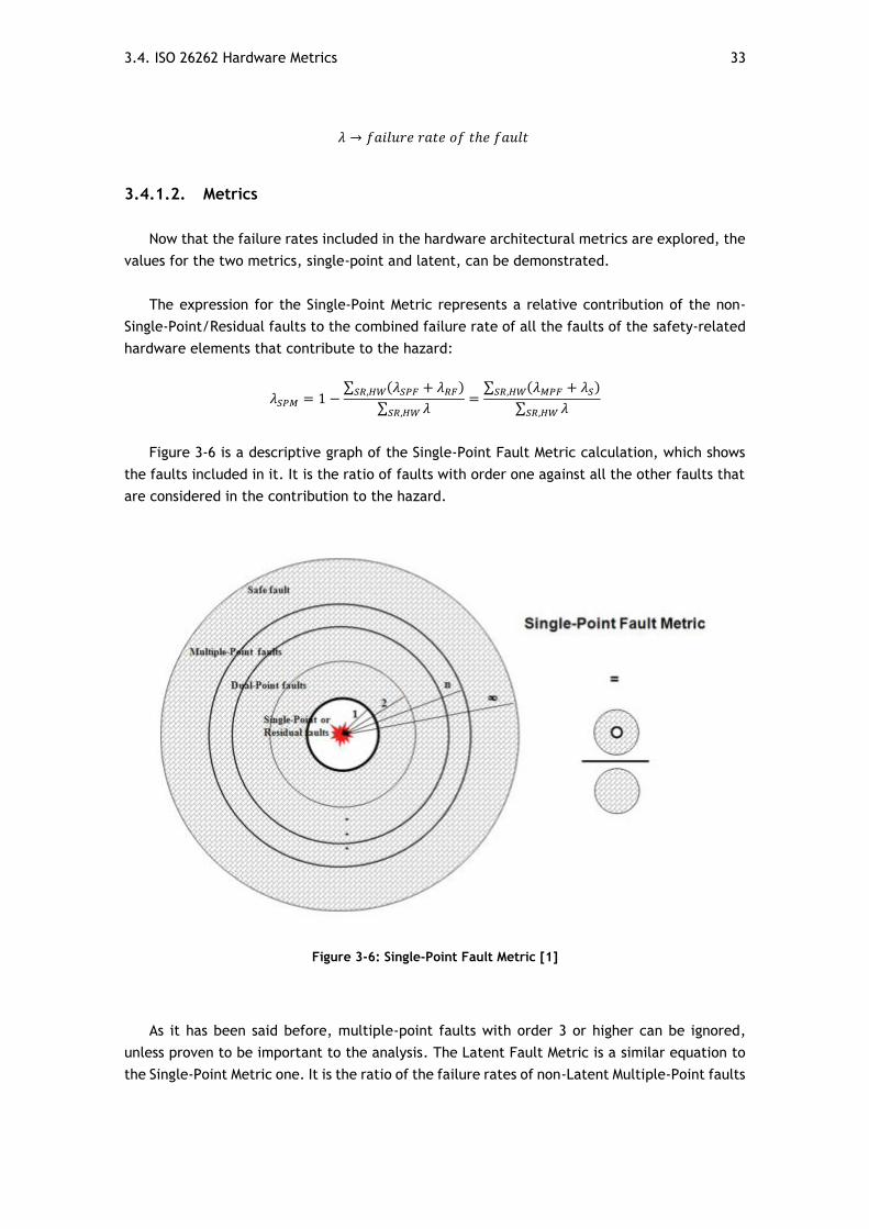
The expression for the Single-Point Metric represents a relative contribution of the non-
Single-Point/Residual faults to the combined failure rate of all the faults of the safety-related
hardware elements that contribute to the hazard:
𝜆𝑆𝑃𝑀 = 1 −∑ (𝜆𝑆𝑃𝐹 + 𝜆𝑅𝐹)𝑆𝑅,𝐻𝑊
∑ 𝜆𝑆𝑅,𝐻𝑊
=∑ (𝜆𝑀𝑃𝐹 + 𝜆𝑆)𝑆𝑅,𝐻𝑊
∑ 𝜆𝑆𝑅,𝐻𝑊
Figure 3-6 is a descriptive graph of the Single-Point Fault Metric calculation, which shows
the faults included in it. It is the ratio of faults with order one against all the other faults that
are considered in the contribution to the hazard.
Figure 3-6: Single-Point Fault Metric [1]
As it has been said before, multiple-point faults with order 3 or higher can be ignored,
unless proven to be important to the analysis. The Latent Fault Metric is a similar equation to
the Single-Point Metric one. It is the ratio of the failure rates of non-Latent Multiple-Point faults
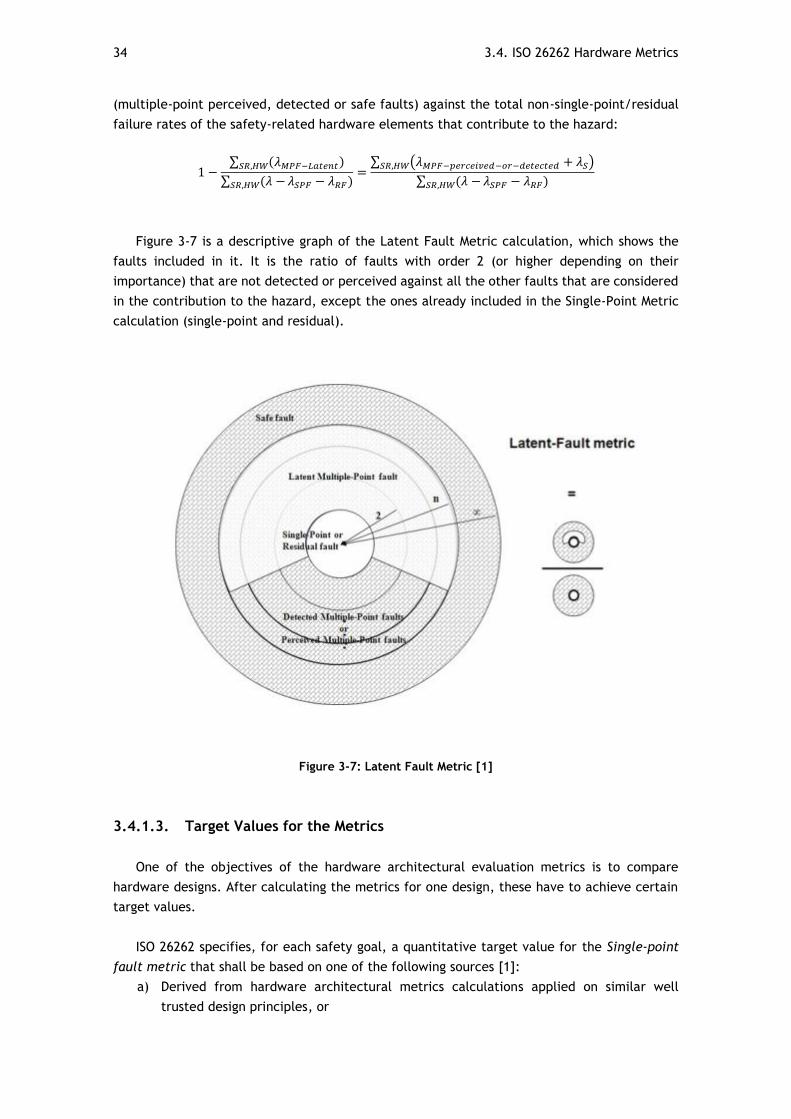
34 3.4. ISO 26262 Hardware Metrics
(multiple-point perceived, detected or safe faults) against the total non-single-point/residual
failure rates of the safety-related hardware elements that contribute to the hazard:
1 −∑ (𝜆𝑀𝑃𝐹−𝐿𝑎𝑡𝑒𝑛𝑡)𝑆𝑅,𝐻𝑊
∑ (𝜆 −𝑆𝑅,𝐻𝑊 𝜆𝑆𝑃𝐹 − 𝜆𝑅𝐹)=
∑ (𝜆𝑀𝑃𝐹−𝑝𝑒𝑟𝑐𝑒𝑖𝑣𝑒𝑑−𝑜𝑟−𝑑𝑒𝑡𝑒𝑐𝑡𝑒𝑑 + 𝜆𝑆)𝑆𝑅,𝐻𝑊
∑ (𝜆 −𝑆𝑅,𝐻𝑊 𝜆𝑆𝑃𝐹 − 𝜆𝑅𝐹)
Figure 3-7 is a descriptive graph of the Latent Fault Metric calculation, which shows the
faults included in it. It is the ratio of faults with order 2 (or higher depending on their
importance) that are not detected or perceived against all the other faults that are considered
in the contribution to the hazard, except the ones already included in the Single-Point Metric
calculation (single-point and residual).
Figure 3-7: Latent Fault Metric [1]
3.4.1.3. Target Values for the Metrics
One of the objectives of the hardware architectural evaluation metrics is to compare
hardware designs. After calculating the metrics for one design, these have to achieve certain
target values.
ISO 26262 specifies, for each safety goal, a quantitative target value for the Single-point
fault metric that shall be based on one of the following sources [1]:
a) Derived from hardware architectural metrics calculations applied on similar well
trusted design principles, or
Evaluation of Safety Goal Violations 35
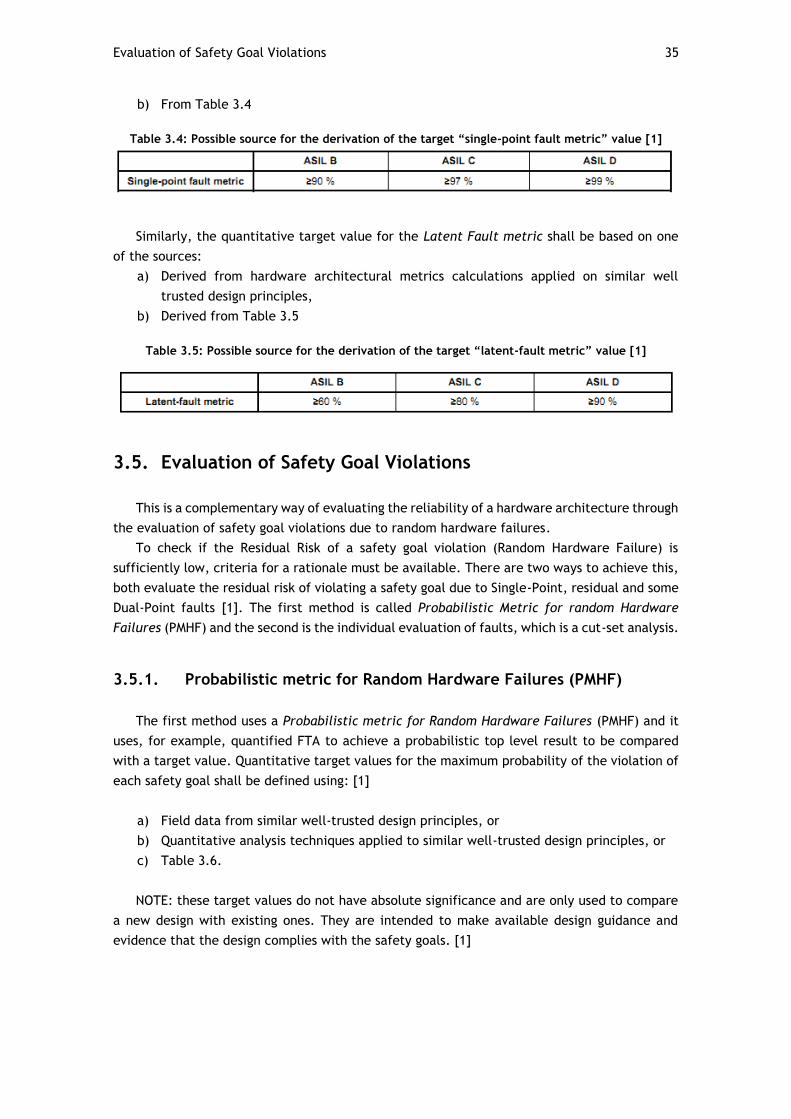
b) From Table 3.4
Table 3.4: Possible source for the derivation of the target “single-point fault metric” value [1]
Similarly, the quantitative target value for the Latent Fault metric shall be based on one
of the sources:
a) Derived from hardware architectural metrics calculations applied on similar well
trusted design principles,
b) Derived from Table 3.5
Table 3.5: Possible source for the derivation of the target “latent-fault metric” value [1]
3.5. Evaluation of Safety Goal Violations
This is a complementary way of evaluating the reliability of a hardware architecture through
the evaluation of safety goal violations due to random hardware failures.
To check if the Residual Risk of a safety goal violation (Random Hardware Failure) is
sufficiently low, criteria for a rationale must be available. There are two ways to achieve this,
both evaluate the residual risk of violating a safety goal due to Single-Point, residual and some
Dual-Point faults [1]. The first method is called Probabilistic Metric for random Hardware
Failures (PMHF) and the second is the individual evaluation of faults, which is a cut-set analysis.
3.5.1. Probabilistic metric for Random Hardware Failures (PMHF)
The first method uses a Probabilistic metric for Random Hardware Failures (PMHF) and it
uses, for example, quantified FTA to achieve a probabilistic top level result to be compared
with a target value. Quantitative target values for the maximum probability of the violation of
each safety goal shall be defined using: [1]
a) Field data from similar well-trusted design principles, or
b) Quantitative analysis techniques applied to similar well-trusted design principles, or
c) Table 3.6.
NOTE: these target values do not have absolute significance and are only used to compare
a new design with existing ones. They are intended to make available design guidance and
evidence that the design complies with the safety goals. [1]
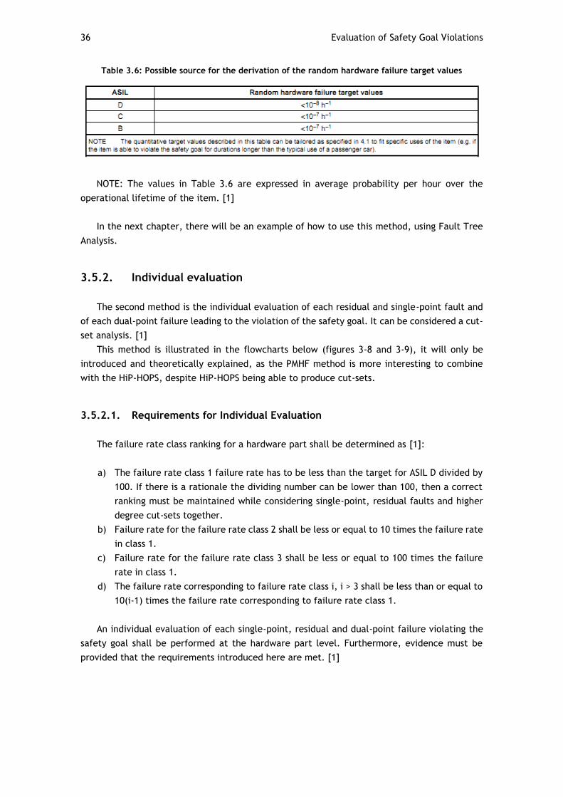
36 Evaluation of Safety Goal Violations
Table 3.6: Possible source for the derivation of the random hardware failure target values
NOTE: The values in Table 3.6 are expressed in average probability per hour over the
operational lifetime of the item. [1]
In the next chapter, there will be an example of how to use this method, using Fault Tree
Analysis.
3.5.2. Individual evaluation
The second method is the individual evaluation of each residual and single-point fault and
of each dual-point failure leading to the violation of the safety goal. It can be considered a cut-
set analysis. [1]
This method is illustrated in the flowcharts below (figures 3-8 and 3-9), it will only be
introduced and theoretically explained, as the PMHF method is more interesting to combine
with the HiP-HOPS, despite HiP-HOPS being able to produce cut-sets.
3.5.2.1. Requirements for Individual Evaluation
The failure rate class ranking for a hardware part shall be determined as [1]:
a) The failure rate class 1 failure rate has to be less than the target for ASIL D divided by
100. If there is a rationale the dividing number can be lower than 100, then a correct
ranking must be maintained while considering single-point, residual faults and higher
degree cut-sets together.
b) Failure rate for the failure rate class 2 shall be less or equal to 10 times the failure rate
in class 1.
c) Failure rate for the failure rate class 3 shall be less or equal to 100 times the failure
rate in class 1.
d) The failure rate corresponding to failure rate class i, i > 3 shall be less than or equal to
10(i-1) times the failure rate corresponding to failure rate class 1.
An individual evaluation of each single-point, residual and dual-point failure violating the
safety goal shall be performed at the hardware part level. Furthermore, evidence must be
provided that the requirements introduced here are met. [1]
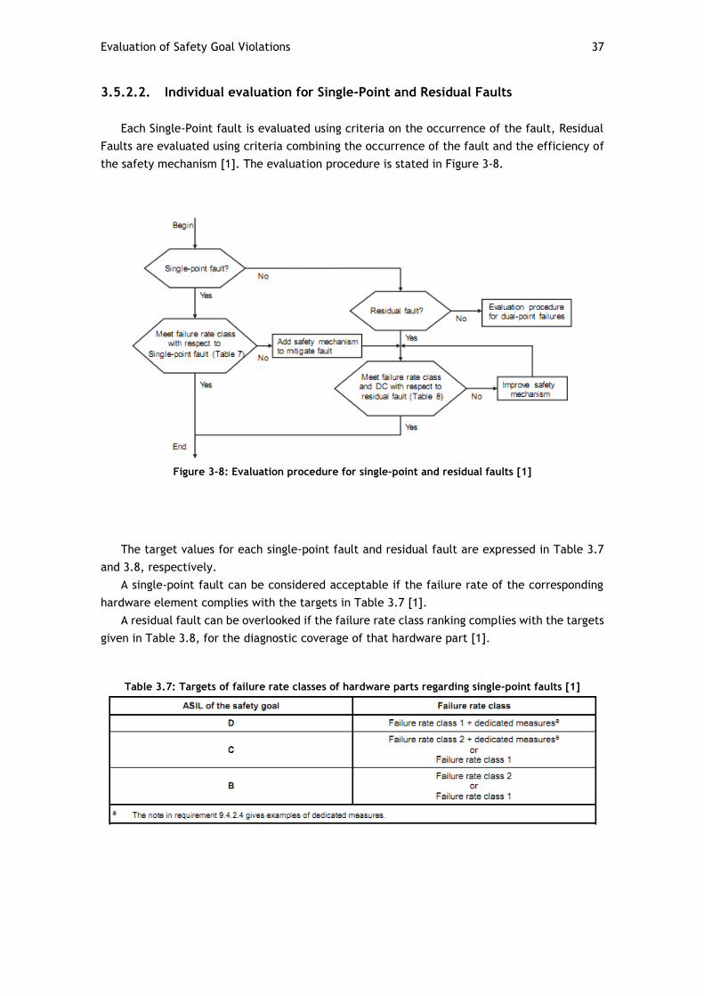
Evaluation of Safety Goal Violations 37
3.5.2.2. Individual evaluation for Single-Point and Residual Faults
Each Single-Point fault is evaluated using criteria on the occurrence of the fault, Residual
Faults are evaluated using criteria combining the occurrence of the fault and the efficiency of
the safety mechanism [1]. The evaluation procedure is stated in Figure 3-8.
Figure 3-8: Evaluation procedure for single-point and residual faults [1]
The target values for each single-point fault and residual fault are expressed in Table 3.7
and 3.8, respectively.
A single-point fault can be considered acceptable if the failure rate of the corresponding
hardware element complies with the targets in Table 3.7 [1].
A residual fault can be overlooked if the failure rate class ranking complies with the targets
given in Table 3.8, for the diagnostic coverage of that hardware part [1].
Table 3.7: Targets of failure rate classes of hardware parts regarding single-point faults [1]
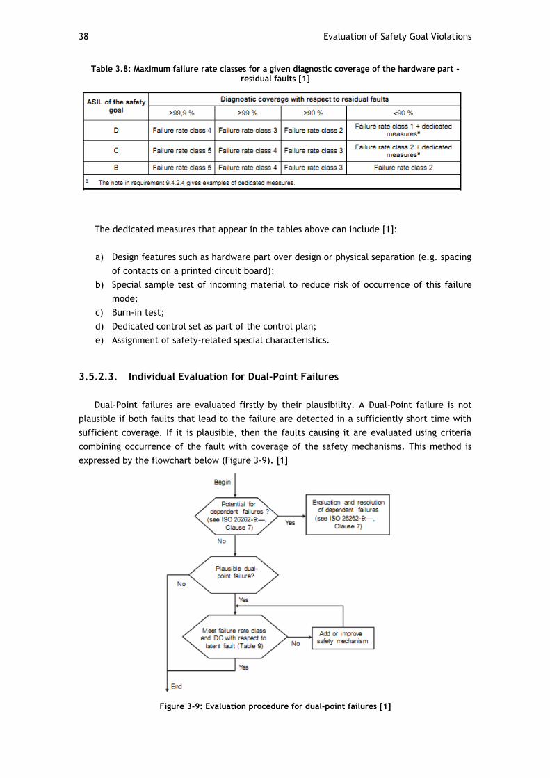
38 Evaluation of Safety Goal Violations
Table 3.8: Maximum failure rate classes for a given diagnostic coverage of the hardware part – residual faults [1]
The dedicated measures that appear in the tables above can include [1]:
a) Design features such as hardware part over design or physical separation (e.g. spacing
of contacts on a printed circuit board);
b) Special sample test of incoming material to reduce risk of occurrence of this failure
mode;
c) Burn-in test;
d) Dedicated control set as part of the control plan;
e) Assignment of safety-related special characteristics.
3.5.2.3. Individual Evaluation for Dual-Point Failures
Dual-Point failures are evaluated firstly by their plausibility. A Dual-Point failure is not
plausible if both faults that lead to the failure are detected in a sufficiently short time with
sufficient coverage. If it is plausible, then the faults causing it are evaluated using criteria
combining occurrence of the fault with coverage of the safety mechanisms. This method is
expressed by the flowchart below (Figure 3-9). [1]
Figure 3-9: Evaluation procedure for dual-point failures [1]
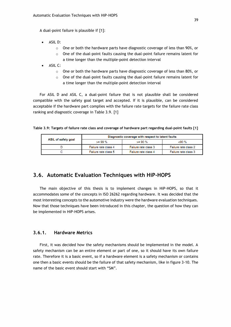
Automatic Evaluation Techniques with HiP-HOPS 39
A dual-point failure is plausible if [1]:
ASIL D:
o One or both the hardware parts have diagnostic coverage of less than 90%, or
o One of the dual-point faults causing the dual-point failure remains latent for
a time longer than the multiple-point detection interval
ASIL C:
o One or both the hardware parts have diagnostic coverage of less than 80%, or
o One of the dual-point faults causing the dual-point failure remains latent for
a time longer than the multiple-point detection interval
For ASIL D and ASIL C, a dual-point failure that is not plausible shall be considered
compatible with the safety goal target and accepted. If it is plausible, can be considered
acceptable if the hardware part complies with the failure rate targets for the failure rate class
ranking and diagnostic coverage in Table 3.9. [1]
Table 3.9: Targets of failure rate class and coverage of hardware part regarding dual-point faults [1]
3.6. Automatic Evaluation Techniques with HiP-HOPS
The main objective of this thesis is to implement changes in HiP-HOPS, so that it
accommodates some of the concepts in ISO 26262 regarding hardware. It was decided that the
most interesting concepts to the automotive industry were the hardware evaluation techniques.
Now that those techniques have been introduced in this chapter, the question of how they can
be implemented in HiP-HOPS arises.
3.6.1. Hardware Metrics
First, it was decided how the safety mechanisms should be implemented in the model. A
safety mechanism can be an entire element or part of one, so it should have its own failure
rate. Therefore it is a basic event, so if a hardware element is a safety mechanism or contains
one then a basic events should be the failure of that safety mechanism, like in figure 3-10. The
name of the basic event should start with “SM”.
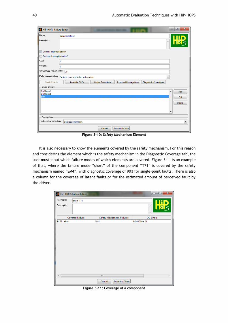
40 Automatic Evaluation Techniques with HiP-HOPS
Figure 3-10: Safety Mechanism Element
It is also necessary to know the elements covered by the safety mechanism. For this reason
and considering the element which is the safety mechanism in the Diagnostic Coverage tab, the
user must input which failure modes of which elements are covered. Figure 3-11 is an example
of that, where the failure mode “short” of the component “T71” is covered by the safety
mechanism named “SM4”, with diagnostic coverage of 90% for single-point faults. There is also
a column for the coverage of latent faults or for the estimated amount of perceived fault by
the driver.
Figure 3-11: Coverage of a component
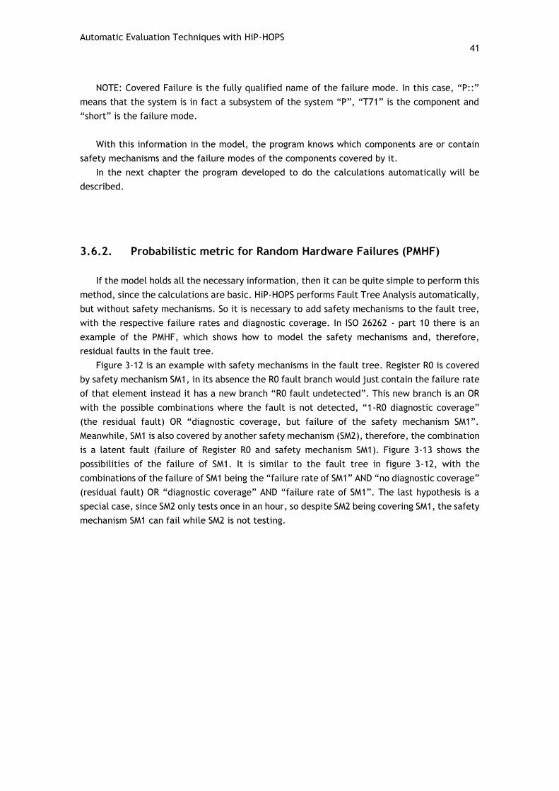
Automatic Evaluation Techniques with HiP-HOPS 41
NOTE: Covered Failure is the fully qualified name of the failure mode. In this case, “P::”
means that the system is in fact a subsystem of the system “P”, “T71” is the component and
“short” is the failure mode.
With this information in the model, the program knows which components are or contain
safety mechanisms and the failure modes of the components covered by it.
In the next chapter the program developed to do the calculations automatically will be
described.
3.6.2. Probabilistic metric for Random Hardware Failures (PMHF)
If the model holds all the necessary information, then it can be quite simple to perform this
method, since the calculations are basic. HiP-HOPS performs Fault Tree Analysis automatically,
but without safety mechanisms. So it is necessary to add safety mechanisms to the fault tree,
with the respective failure rates and diagnostic coverage. In ISO 26262 - part 10 there is an
example of the PMHF, which shows how to model the safety mechanisms and, therefore,
residual faults in the fault tree.
Figure 3-12 is an example with safety mechanisms in the fault tree. Register R0 is covered
by safety mechanism SM1, in its absence the R0 fault branch would just contain the failure rate
of that element instead it has a new branch “R0 fault undetected”. This new branch is an OR
with the possible combinations where the fault is not detected, “1-R0 diagnostic coverage”
(the residual fault) OR “diagnostic coverage, but failure of the safety mechanism SM1”.
Meanwhile, SM1 is also covered by another safety mechanism (SM2), therefore, the combination
is a latent fault (failure of Register R0 and safety mechanism SM1). Figure 3-13 shows the
possibilities of the failure of SM1. It is similar to the fault tree in figure 3-12, with the
combinations of the failure of SM1 being the “failure rate of SM1” AND “no diagnostic coverage”
(residual fault) OR “diagnostic coverage” AND “failure rate of SM1”. The last hypothesis is a
special case, since SM2 only tests once in an hour, so despite SM2 being covering SM1, the safety
mechanism SM1 can fail while SM2 is not testing.
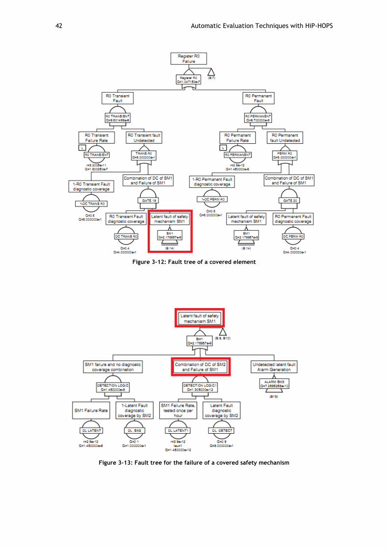
42 Automatic Evaluation Techniques with HiP-HOPS
Figure 3-12: Fault tree of a covered element
Figure 3-13: Fault tree for the failure of a covered safety mechanism
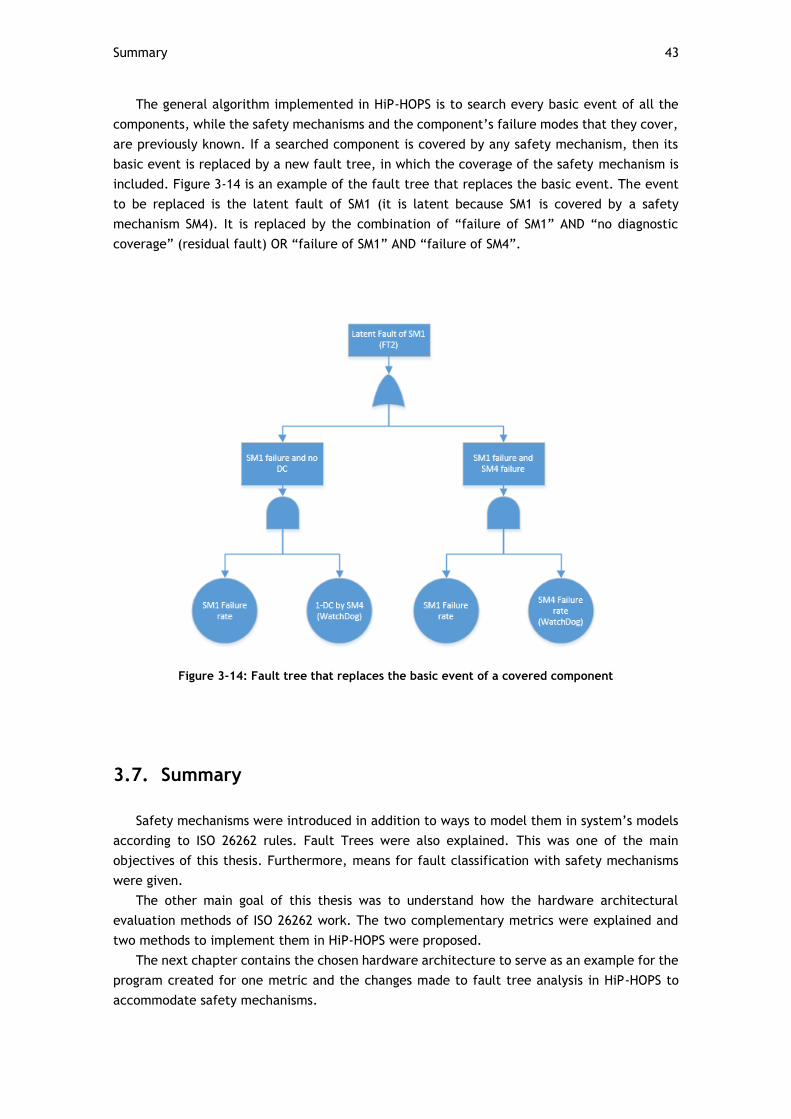
Summary 43
The general algorithm implemented in HiP-HOPS is to search every basic event of all the
components, while the safety mechanisms and the component’s failure modes that they cover,
are previously known. If a searched component is covered by any safety mechanism, then its
basic event is replaced by a new fault tree, in which the coverage of the safety mechanism is
included. Figure 3-14 is an example of the fault tree that replaces the basic event. The event
to be replaced is the latent fault of SM1 (it is latent because SM1 is covered by a safety
mechanism SM4). It is replaced by the combination of “failure of SM1” AND “no diagnostic
coverage” (residual fault) OR “failure of SM1” AND “failure of SM4”.
Figure 3-14: Fault tree that replaces the basic event of a covered component
3.7. Summary
Safety mechanisms were introduced in addition to ways to model them in system’s models
according to ISO 26262 rules. Fault Trees were also explained. This was one of the main
objectives of this thesis. Furthermore, means for fault classification with safety mechanisms
were given.
The other main goal of this thesis was to understand how the hardware architectural
evaluation methods of ISO 26262 work. The two complementary metrics were explained and
two methods to implement them in HiP-HOPS were proposed.
The next chapter contains the chosen hardware architecture to serve as an example for the
program created for one metric and the changes made to fault tree analysis in HiP-HOPS to
accommodate safety mechanisms.

44 Summary
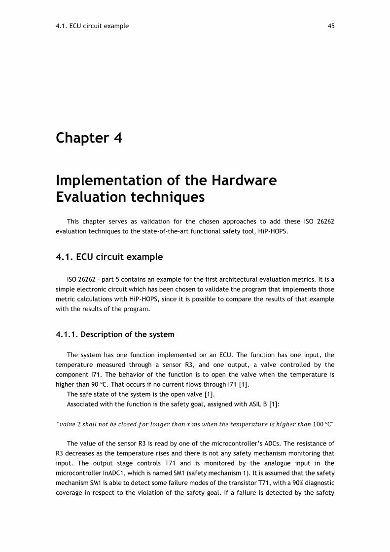
4.1. ECU circuit example 45
Chapter 4
Implementation of the Hardware Evaluation techniques
This chapter serves as validation for the chosen approaches to add these ISO 26262
evaluation techniques to the state-of-the-art functional safety tool, HiP-HOPS.
4.1. ECU circuit example
ISO 26262 – part 5 contains an example for the first architectural evaluation metrics. It is a
simple electronic circuit which has been chosen to validate the program that implements those
metric calculations with HiP-HOPS, since it is possible to compare the results of that example
with the results of the program.
4.1.1. Description of the system
The system has one function implemented on an ECU. The function has one input, the
temperature measured through a sensor R3, and one output, a valve controlled by the
component I71. The behavior of the function is to open the valve when the temperature is
higher than 90 ºC. That occurs if no current flows through I71 [1].
The safe state of the system is the open valve [1].
Associated with the function is the safety goal, assigned with ASIL B [1]:
"𝑣𝑎𝑙𝑣𝑒 2 𝑠ℎ𝑎𝑙𝑙 𝑛𝑜𝑡 𝑏𝑒 𝑐𝑙𝑜𝑠𝑒𝑑 𝑓𝑜𝑟 𝑙𝑜𝑛𝑔𝑒𝑟 𝑡ℎ𝑎𝑛 𝑥 𝑚𝑠 𝑤ℎ𝑒𝑛 𝑡ℎ𝑒 𝑡𝑒𝑚𝑝𝑒𝑟𝑎𝑡𝑢𝑟𝑒 𝑖𝑠 ℎ𝑖𝑔ℎ𝑒𝑟 𝑡ℎ𝑎𝑛 100 ℃"
The value of the sensor R3 is read by one of the microcontroller’s ADCs. The resistance of
R3 decreases as the temperature rises and there is not any safety mechanism monitoring that
input. The output stage controls T71 and is monitored by the analogue input in the
microcontroller InADC1, which is named SM1 (safety mechanism 1). It is assumed that the safety
mechanism SM1 is able to detect some failure modes of the transistor T71, with a 90% diagnostic
coverage in respect to the violation of the safety goal. If a failure is detected by the safety
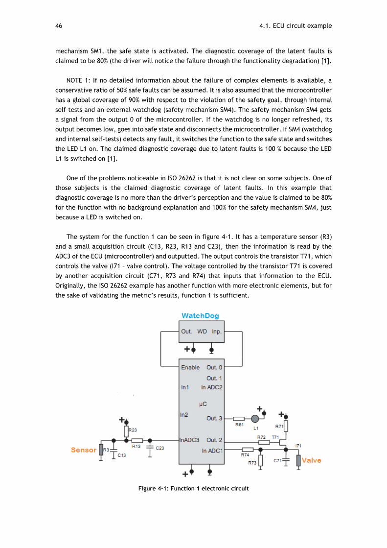
46 4.1. ECU circuit example
mechanism SM1, the safe state is activated. The diagnostic coverage of the latent faults is
claimed to be 80% (the driver will notice the failure through the functionality degradation) [1].
NOTE 1: If no detailed information about the failure of complex elements is available, a
conservative ratio of 50% safe faults can be assumed. It is also assumed that the microcontroller
has a global coverage of 90% with respect to the violation of the safety goal, through internal
self-tests and an external watchdog (safety mechanism SM4). The safety mechanism SM4 gets
a signal from the output 0 of the microcontroller. If the watchdog is no longer refreshed, its
output becomes low, goes into safe state and disconnects the microcontroller. If SM4 (watchdog
and internal self-tests) detects any fault, it switches the function to the safe state and switches
the LED L1 on. The claimed diagnostic coverage due to latent faults is 100 % because the LED
L1 is switched on [1].
One of the problems noticeable in ISO 26262 is that it is not clear on some subjects. One of
those subjects is the claimed diagnostic coverage of latent faults. In this example that
diagnostic coverage is no more than the driver’s perception and the value is claimed to be 80%
for the function with no background explanation and 100% for the safety mechanism SM4, just
because a LED is switched on.
The system for the function 1 can be seen in figure 4-1. It has a temperature sensor (R3)
and a small acquisition circuit (C13, R23, R13 and C23), then the information is read by the
ADC3 of the ECU (microcontroller) and outputted. The output controls the transistor T71, which
controls the valve (I71 – valve control). The voltage controlled by the transistor T71 is covered
by another acquisition circuit (C71, R73 and R74) that inputs that information to the ECU.
Originally, the ISO 26262 example has another function with more electronic elements, but for
the sake of validating the metric’s results, function 1 is sufficient.
Figure 4-1: Function 1 electronic circuit

4.1. ECU circuit example 47
There is also a table (Table 4.1) describing the failure behavior of the components, the
diagnostic coverage and other relevant information. The developed metric calculation program
is able to reproduce a table like that in excel format, through the model information.
Table 4.1: Failure information for the system [1]
48 4.1. ECU circuit example
4.1.2. Failure Model
To work with HiP-HOPS it is necessary to model the system described above. It is not a
functional model, but a failure propagation model, which contains information about the failure
behavior of the components and the connections for the failure propagation. The model can be
created with Matlab Simulink, Eclipse-based UML tools and ITI SimulationX. For this thesis
Simulink is used due to previous experience with it. The created model can be seen in Figure
4-2. The model has got to have the proper physical connections to allow correct failure
propagation, however it does not simulate the system’s operation.
NOTE 1: The model is actually a sub-system inside an abstraction block named Perspective,
which acts as the environment, to allow for external events (such as atmospheric conditions,
electrical stress, etc.).
To understand how an electronic system can fail, the designer has to perform circuit
analysis. This can be a difficult task for complex systems, however, this is not one of those and
some information is already given in the ISO 26262 example. The only difficulty encountered
while analyzing this system is the lack of information about the components, for example, in
Table 4.1, they state that if R23 is in short circuit, then the safety goal is violated. It can be
assumed that the safety goal is violated because the input value to the ECU is influenced,
however that would depend on the value of the components that constitute the acquisition
circuit.
Figure 4-2: Failure Propagation Model
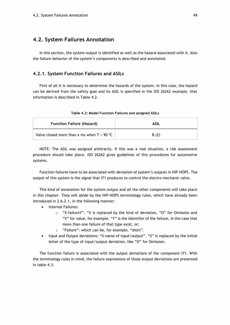
4.2. System Failures Annotation 49
4.2. System Failures Annotation
In this section, the system output is identified as well as the hazard associated with it. Also
the failure behavior of the system’s components is described and annotated.
4.2.1. System Function Failures and ASILs
First of all it is necessary to determine the hazards of the system. In this case, the hazard
can be derived from the safety goal and its ASIL is specified in the ISO 26262 example, that
information is described in Table 4.2.
Table 4.2: Model Function Failures and assigned ASILs
Function Failure (Hazard) ASIL
Valve closed more than x ms when T > 90 ºC B (2)
NOTE: The ASIL was assigned arbitrarily. If this was a real situation, a risk assessment
procedure should take place. ISO 26262 gives guidelines of this procedures for automotive
systems.
Function failures have to be associated with deviation of system’s outputs in HiP-HOPS. The
output of this system is the signal that I71 produces to control the electro mechanic valve.
This kind of annotation for the system output and all the other components will take place
in this chapter. They will abide by the HiP-HOPS terminology rules, which have already been
introduced in 2.6.2.1, in the following manner:
Internal Failures:
o “X-failureY”. “X is replaced by the kind of deviation, “O” for Omission and
“V” for value, for example. “Y” is the identifier of the failure, in the case that
more than one failure of that type exist, or;
o “Failure”: which can be, for example, “short”.
Input and Output deviations: “X-name of input/output”. “X” is replaced by the initial
letter of the type of input/output deviation, like “O” for Omission.
The function failure is associated with the output deviations of the component I71. With
the terminology rules in mind, the failure expressions of those output deviations are presented
in table 4.3.
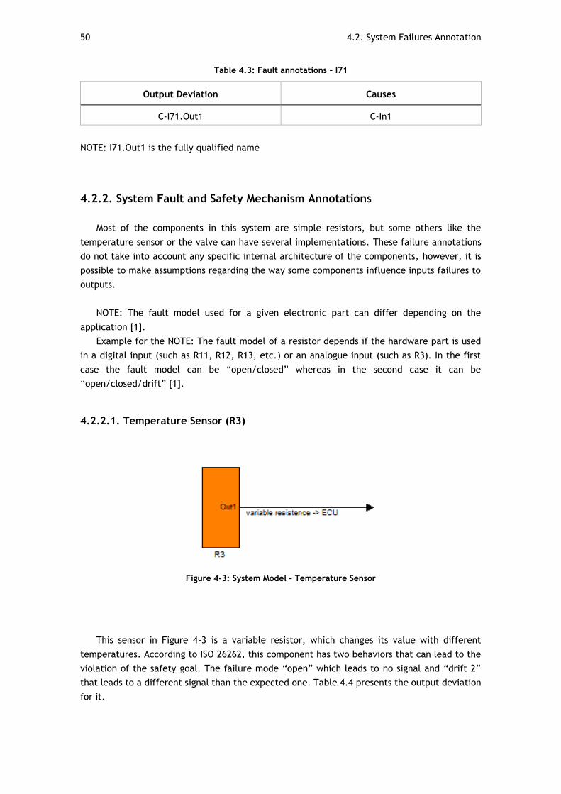
50 4.2. System Failures Annotation
Table 4.3: Fault annotations – I71
Output Deviation Causes
C-I71.Out1 C-In1
NOTE: I71.Out1 is the fully qualified name
4.2.2. System Fault and Safety Mechanism Annotations
Most of the components in this system are simple resistors, but some others like the
temperature sensor or the valve can have several implementations. These failure annotations
do not take into account any specific internal architecture of the components, however, it is
possible to make assumptions regarding the way some components influence inputs failures to
outputs.
NOTE: The fault model used for a given electronic part can differ depending on the
application [1].
Example for the NOTE: The fault model of a resistor depends if the hardware part is used
in a digital input (such as R11, R12, R13, etc.) or an analogue input (such as R3). In the first
case the fault model can be “open/closed” whereas in the second case it can be
“open/closed/drift” [1].
4.2.2.1. Temperature Sensor (R3)
Figure 4-3: System Model – Temperature Sensor
This sensor in Figure 4-3 is a variable resistor, which changes its value with different
temperatures. According to ISO 26262, this component has two behaviors that can lead to the
violation of the safety goal. The failure mode “open” which leads to no signal and “drift 2”
that leads to a different signal than the expected one. Table 4.4 presents the output deviation
for it.

4.2. System Failures Annotation 51
Table 4.4: Fault Annotations – Temperature Sensor
Output Deviation Causes
V-Out1 drift2
O-Out1 open
4.2.2.2. Signal Acquisition Circuit
This circuit exists to formulate a desirable range for the input signal (depending on the
temperature sensor internal architecture) to be correctly associated with a temperature value
in the ECU. The circuit is presented in Figure 4-4 and the failure annotations of its components
will be presented in the next tables.
Figure 4-4: System Model – Signal Acquisition Circuit
Table 4.5: Failure Annotations – C13
Output Deviation Causes
V-Out1 open
The purpose of the capacitor C13 is ESD protection. The failure mode open circuit means
loss of protection [1].
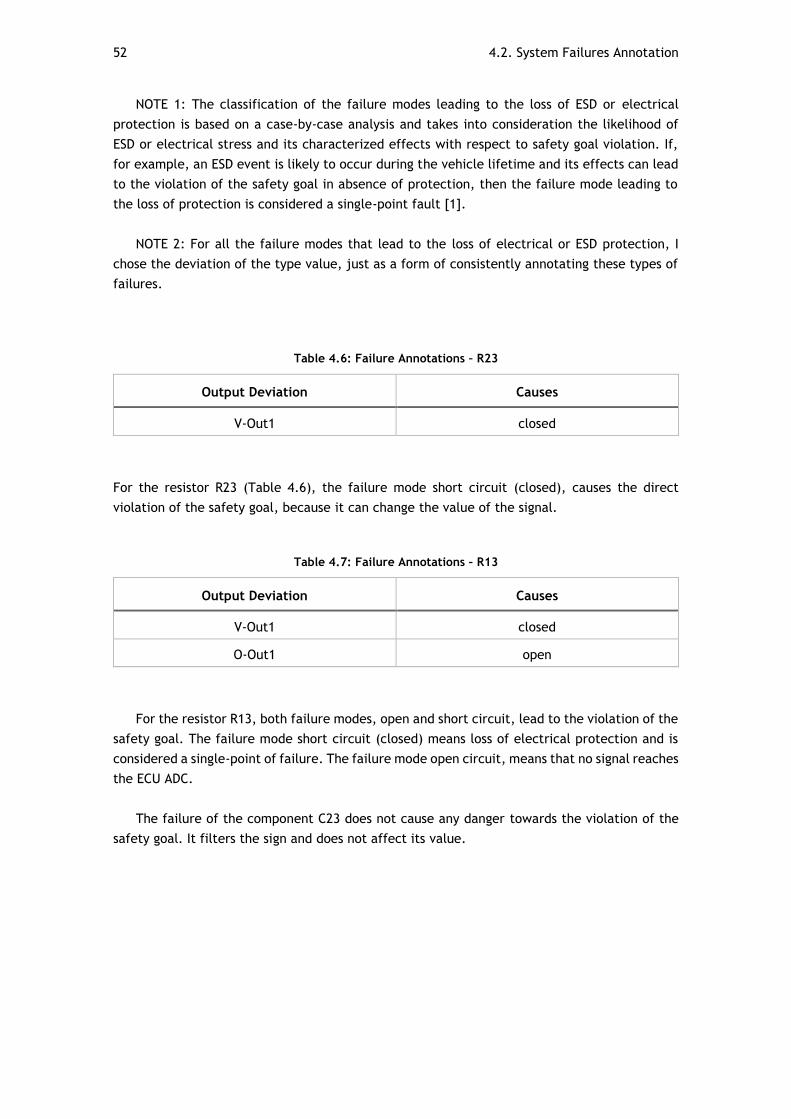
52 4.2. System Failures Annotation
NOTE 1: The classification of the failure modes leading to the loss of ESD or electrical
protection is based on a case-by-case analysis and takes into consideration the likelihood of
ESD or electrical stress and its characterized effects with respect to safety goal violation. If,
for example, an ESD event is likely to occur during the vehicle lifetime and its effects can lead
to the violation of the safety goal in absence of protection, then the failure mode leading to
the loss of protection is considered a single-point fault [1].
NOTE 2: For all the failure modes that lead to the loss of electrical or ESD protection, I
chose the deviation of the type value, just as a form of consistently annotating these types of
failures.
Table 4.6: Failure Annotations – R23
Output Deviation Causes
V-Out1 closed
For the resistor R23 (Table 4.6), the failure mode short circuit (closed), causes the direct
violation of the safety goal, because it can change the value of the signal.
Table 4.7: Failure Annotations – R13
Output Deviation Causes
V-Out1 closed
O-Out1 open
For the resistor R13, both failure modes, open and short circuit, lead to the violation of the
safety goal. The failure mode short circuit (closed) means loss of electrical protection and is
considered a single-point of failure. The failure mode open circuit, means that no signal reaches
the ECU ADC.
The failure of the component C23 does not cause any danger towards the violation of the
safety goal. It filters the sign and does not affect its value.
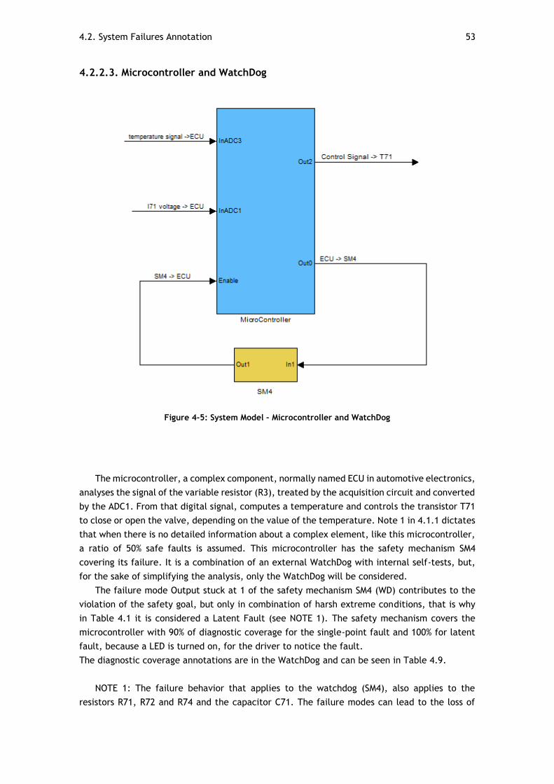
4.2. System Failures Annotation 53
4.2.2.3. Microcontroller and WatchDog
Figure 4-5: System Model – Microcontroller and WatchDog
The microcontroller, a complex component, normally named ECU in automotive electronics,
analyses the signal of the variable resistor (R3), treated by the acquisition circuit and converted
by the ADC1. From that digital signal, computes a temperature and controls the transistor T71
to close or open the valve, depending on the value of the temperature. Note 1 in 4.1.1 dictates
that when there is no detailed information about a complex element, like this microcontroller,
a ratio of 50% safe faults is assumed. This microcontroller has the safety mechanism SM4
covering its failure. It is a combination of an external WatchDog with internal self-tests, but,
for the sake of simplifying the analysis, only the WatchDog will be considered.
The failure mode Output stuck at 1 of the safety mechanism SM4 (WD) contributes to the
violation of the safety goal, but only in combination of harsh extreme conditions, that is why
in Table 4.1 it is considered a Latent Fault (see NOTE 1). The safety mechanism covers the
microcontroller with 90% of diagnostic coverage for the single-point fault and 100% for latent
fault, because a LED is turned on, for the driver to notice the fault.
The diagnostic coverage annotations are in the WatchDog and can be seen in Table 4.9.
NOTE 1: The failure behavior that applies to the watchdog (SM4), also applies to the
resistors R71, R72 and R74 and the capacitor C71. The failure modes can lead to the loss of
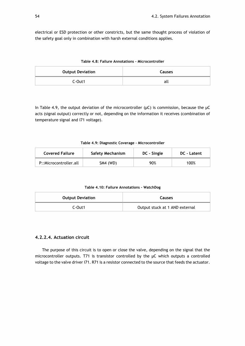
54 4.2. System Failures Annotation
electrical or ESD protection or other constricts, but the same thought process of violation of
the safety goal only in combination with harsh external conditions applies.
Table 4.8: Failure Annotations - Microcontroller
Output Deviation Causes
C-Out1 all
In Table 4.9, the output deviation of the microcontroller (µC) is commission, because the µC
acts (signal output) correctly or not, depending on the information it receives (combination of
temperature signal and I71 voltage).
Table 4.9: Diagnostic Coverage - Microcontroller
Covered Failure Safety Mechanism DC - Single DC - Latent
P::Microcontroller.all SM4 (WD) 90% 100%
Table 4.10: Failure Annotations - WatchDog
Output Deviation Causes
C-Out1 Output stuck at 1 AND external
4.2.2.4. Actuation circuit
The purpose of this circuit is to open or close the valve, depending on the signal that the
microcontroller outputs. T71 is transistor controlled by the µC which outputs a controlled
voltage to the valve driver I71. R71 is a resistor connected to the source that feeds the actuator.
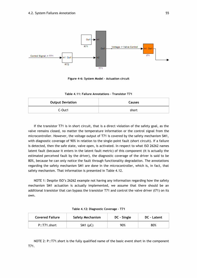
4.2. System Failures Annotation 55
Figure 4-6: System Model – Actuation circuit
Table 4.11: Failure Annotations – Transistor T71
Output Deviation Causes
C-Out1 short
If the transistor T71 is in short circuit, that is a direct violation of the safety goal, as the
valve remains closed, no matter the temperature information or the control signal from the
microcontroller. However, the voltage output of T71 is covered by the safety mechanism SM1,
with diagnostic coverage of 90% in relation to the single-point fault (short circuit). If a failure
is detected, then the safe state, valve open, is activated. In respect to what ISO 26262 names
latent fault (because it enters in the latent fault metric) of this component (it is actually the
estimated perceived fault by the driver), the diagnostic coverage of the driver is said to be
80%, because he can only notice the fault through functionality degradation. The annotations
regarding the safety mechanism SM1 are done in the microcontroller, which is, in fact, that
safety mechanism. That information is presented in Table 4.12.
NOTE 1: Despite ISO’s 26262 example not having any information regarding how the safety
mechanism SM1 actuation is actually implemented, we assume that there should be an
additional transistor that can bypass the transistor T71 and control the valve driver (I71) on its
own.
Table 4.12: Diagnostic Coverage – T71
Covered Failure Safety Mechanism DC - Single DC - Latent
P::T71.short SM1 (µC) 90% 80%
NOTE 2: P::T71.short is the fully qualified name of the basic event short in the component
T71.
56 4.2. System Failures Annotation
Table 4.13: Failure Annotations – R72
Output Deviation Causes
C-Out1 closed and external
The resistor R72 has two possible failure modes, open or short circuit, however, the open
circuit of this component does not contribute to the violation of the safety goal, since the valve
will be open (safe state) because the transistor remains open. If the component is in short
circuit, that leads to the loss of electrical protection. The safety goal is violated if that failure
mode occurs and harsh external conditions apply, hence the reason why in Table 4.1, this is a
latent failure (see NOTE 1 in 4.2.2.3).
Table 4.14: Failure Annotations – R71
Output Deviation Causes
C-Out1 closed and external
If the component I71 (valve driver) fails, that has no effect regarding the violation of the
safety goal, as the valve will remain in its safe state, open.
4.2.2.5. Signal Acquisition Circuit 2 – Safety Mechanism SM1
Figure 4-7: System Model – Signal Acquisition Circuit 2 (SM1)
This acquisition circuit is to modulate the voltage in I71 to be inputted by the ADC1 in the
microcontroller. The failure annotations for its components are going to be presented in the
next few tables.
4.2. System Failures Annotation 57
The resistor R73 has no effect regarding the safety goal violation as it is merely a component
to perform tension division.
Table 4.15: Failure Annotations – C71
Output Deviation Causes
C-Out1 open and external
The failure mode open circuit of this component, means loss of ESD protection. That failure
dictates that the component stays latent. It violates the safety goal if it is latent and certain
external conditions happen.
Table 4.16: Failure Annotations – R74
Output Deviation Causes
V-Out1 closed and external
O-Out1 open and external
The failure mode short circuit (closed) means loss of electrical protection, that fault in
combination with certain external conditions leads to the violation of the safety goal. The other
mode, open circuit also leads to the violation of the safety goal in combination with external
conditions. This last failure mode contributes to an omission type of output deviation, as no
value reaches the microcontroller’s ADC.
IMPORTANT NOTE: Certain components need to have, as causes of output deviation, the
inputs. That allows failure propagation.
Example of NOTE: The valve controller I71 needs to propagate the failures of the
components that are behind it, to its output (system output). So its causes of output deviation,
for the purposes of failure propagation, are the ones presented in Table 4.17.
Table 4.17: Failure Propagation Example – I71
Output Deviation Causes
C-Out1 C-In1
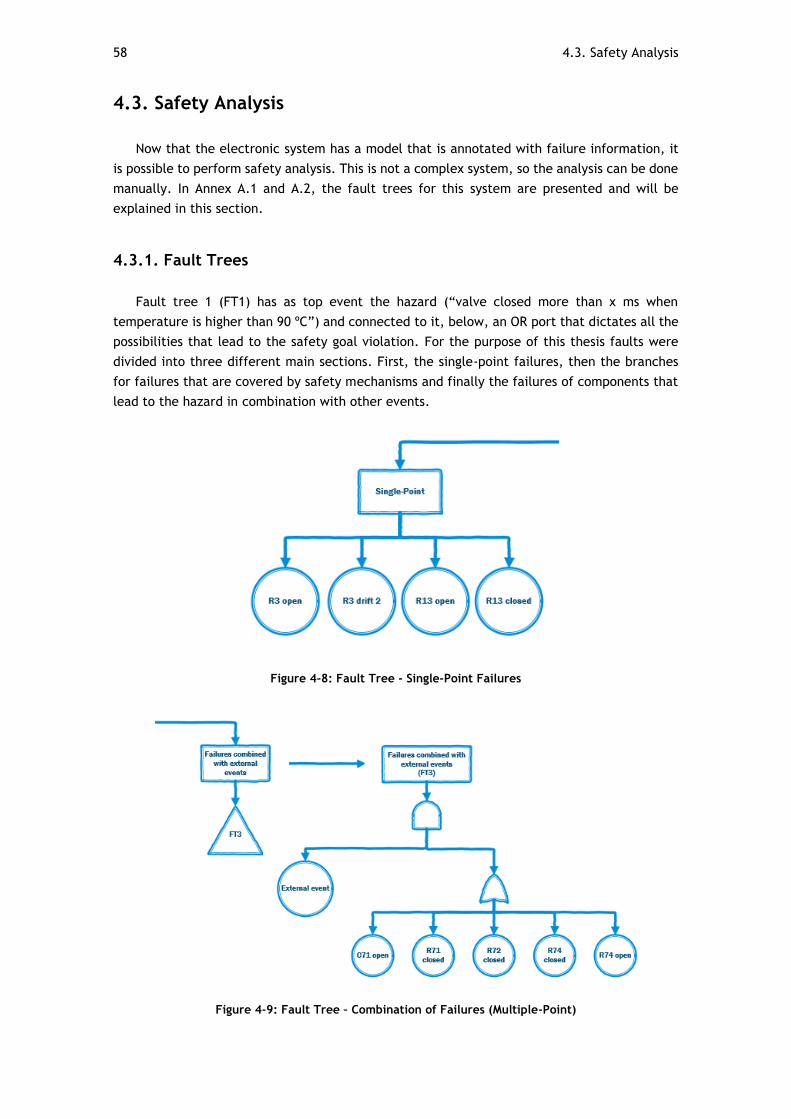
58 4.3. Safety Analysis
4.3. Safety Analysis
Now that the electronic system has a model that is annotated with failure information, it
is possible to perform safety analysis. This is not a complex system, so the analysis can be done
manually. In Annex A.1 and A.2, the fault trees for this system are presented and will be
explained in this section.
4.3.1. Fault Trees
Fault tree 1 (FT1) has as top event the hazard (“valve closed more than x ms when
temperature is higher than 90 ºC”) and connected to it, below, an OR port that dictates all the
possibilities that lead to the safety goal violation. For the purpose of this thesis faults were
divided into three different main sections. First, the single-point failures, then the branches
for failures that are covered by safety mechanisms and finally the failures of components that
lead to the hazard in combination with other events.
Figure 4-8: Fault Tree - Single-Point Failures
Figure 4-9: Fault Tree – Combination of Failures (Multiple-Point)
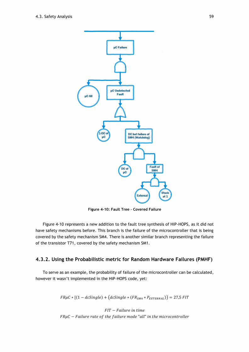
4.3. Safety Analysis 59
Figure 4-10: Fault Tree – Covered Failure
Figure 4-10 represents a new addition to the fault tree synthesis of HiP-HOPS, as it did not
have safety mechanisms before. This branch is the failure of the microcontroller that is being
covered by the safety mechanism SM4. There is another similar branch representing the failure
of the transistor T71, covered by the safety mechanism SM1.
4.3.2. Using the Probabilistic metric for Random Hardware Failures (PMHF)
To serve as an example, the probability of failure of the microcontroller can be calculated,
however it wasn’t implemented in the HiP-HOPS code, yet:
𝐹𝑅𝜇𝐶 ∗ [(1 − 𝑑𝑐𝑆𝑖𝑛𝑔𝑙𝑒) + (𝑑𝑐𝑆𝑖𝑛𝑔𝑙𝑒 ∗ (𝐹𝑅𝑆𝑀4 ∗ 𝑃𝐸𝑋𝑇𝐸𝑅𝑁𝐴𝐿)) = 27,5 𝐹𝐼𝑇
𝐹𝐼𝑇 − 𝐹𝑎𝑖𝑙𝑢𝑟𝑒 𝑖𝑛 𝑡𝑖𝑚𝑒
𝐹𝑅𝜇𝐶 − 𝐹𝑎𝑖𝑙𝑢𝑟𝑒 𝑟𝑎𝑡𝑒 𝑜𝑓 𝑡ℎ𝑒 𝑓𝑎𝑖𝑙𝑢𝑟𝑒 𝑚𝑜𝑑𝑒 "𝑎𝑙𝑙" 𝑖𝑛 𝑡ℎ𝑒 𝑚𝑖𝑐𝑟𝑜𝑐𝑜𝑛𝑡𝑟𝑜𝑙𝑙𝑒𝑟
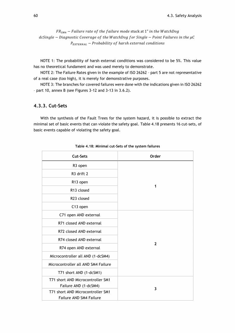
60 4.3. Safety Analysis
𝐹𝑅𝑆𝑀4 − 𝐹𝑎𝑖𝑙𝑢𝑟𝑒 𝑟𝑎𝑡𝑒 𝑜𝑓 𝑡ℎ𝑒 𝑓𝑎𝑖𝑙𝑢𝑟𝑒 𝑚𝑜𝑑𝑒 stuck at 1" 𝑖𝑛 𝑡ℎ𝑒 𝑊𝑎𝑡𝑐ℎ𝐷𝑜𝑔
𝑑𝑐𝑆𝑖𝑛𝑔𝑙𝑒 − 𝐷𝑖𝑎𝑔𝑛𝑜𝑠𝑡𝑖𝑐 𝐶𝑜𝑣𝑒𝑟𝑎𝑔𝑒 𝑜𝑓 𝑡ℎ𝑒 𝑊𝑎𝑡𝑐ℎ𝐷𝑜𝑔 𝑓𝑜𝑟 𝑆𝑖𝑛𝑔𝑙𝑒 − 𝑃𝑜𝑖𝑛𝑡 𝐹𝑎𝑖𝑙𝑢𝑟𝑒𝑠 𝑖𝑛 𝑡ℎ𝑒 𝜇𝐶
𝑃𝐸𝑋𝑇𝐸𝑅𝑁𝐴𝐿 − 𝑃𝑟𝑜𝑏𝑎𝑏𝑖𝑙𝑖𝑡𝑦 𝑜𝑓 ℎ𝑎𝑟𝑠ℎ 𝑒𝑥𝑡𝑒𝑟𝑛𝑎𝑙 𝑐𝑜𝑛𝑑𝑖𝑡𝑖𝑜𝑛𝑠
NOTE 1: The probability of harsh external conditions was considered to be 5%. This value
has no theoretical fundament and was used merely to demonstrate.
NOTE 2: The Failure Rates given in the example of ISO 26262 – part 5 are not representative
of a real case (too high), it is merely for demonstrative purposes.
NOTE 3: The branches for covered failures were done with the indications given in ISO 26262
– part 10, annex B (see Figures 3-12 and 3-13 in 3.6.2).
4.3.3. Cut-Sets
With the synthesis of the Fault Trees for the system hazard, it is possible to extract the
minimal set of basic events that can violate the safety goal. Table 4.18 presents 16 cut-sets, of
basic events capable of violating the safety goal.
Table 4.18: Minimal cut-Sets of the system failures
Cut-Sets Order
R3 open
1
R3 drift 2
R13 open
R13 closed
R23 closed
C13 open
C71 open AND external
2
R71 closed AND external
R72 closed AND external
R74 closed AND external
R74 open AND external
Microcontroller all AND (1-dcSM4)
Microcontroller all AND SM4 Failure
T71 short AND (1-dcSM1)
T71 short AND Microcontroller SM1
Failure AND (1-dcSM4) 3
T71 short AND Microcontroller SM1
Failure AND SM4 Failure
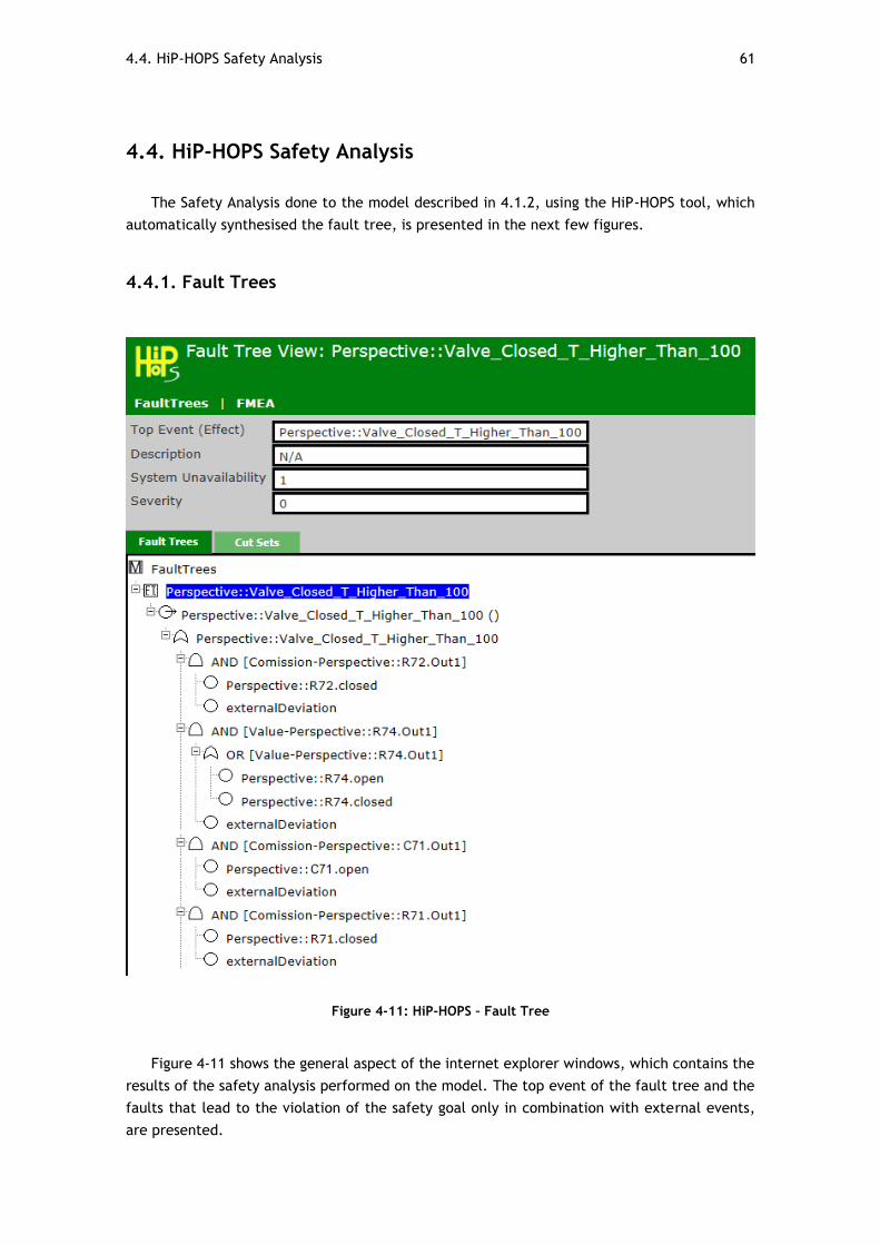
4.4. HiP-HOPS Safety Analysis 61
4.4. HiP-HOPS Safety Analysis
The Safety Analysis done to the model described in 4.1.2, using the HiP-HOPS tool, which
automatically synthesised the fault tree, is presented in the next few figures.
4.4.1. Fault Trees
Figure 4-11: HiP-HOPS – Fault Tree
Figure 4-11 shows the general aspect of the internet explorer windows, which contains the
results of the safety analysis performed on the model. The top event of the fault tree and the
faults that lead to the violation of the safety goal only in combination with external events,
are presented.
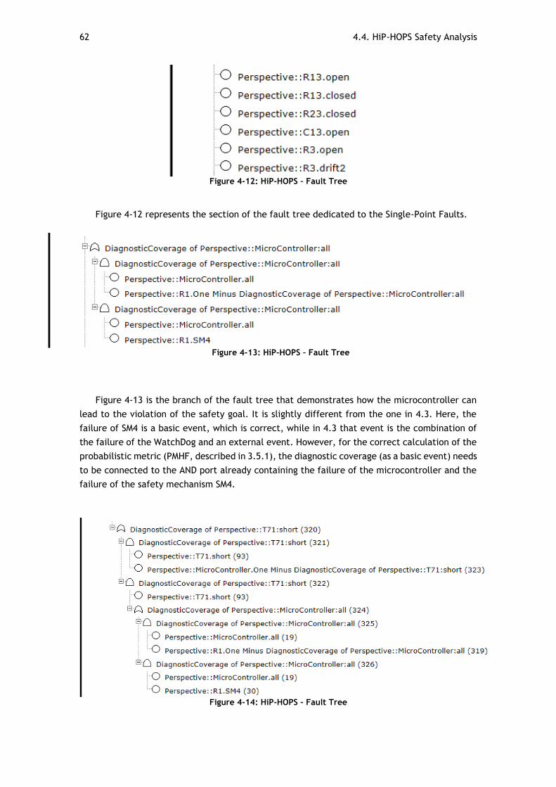
62 4.4. HiP-HOPS Safety Analysis
Figure 4-12: HiP-HOPS – Fault Tree
Figure 4-12 represents the section of the fault tree dedicated to the Single-Point Faults.
Figure 4-13 is the branch of the fault tree that demonstrates how the microcontroller can
lead to the violation of the safety goal. It is slightly different from the one in 4.3. Here, the
failure of SM4 is a basic event, which is correct, while in 4.3 that event is the combination of
the failure of the WatchDog and an external event. However, for the correct calculation of the
probabilistic metric (PMHF, described in 3.5.1), the diagnostic coverage (as a basic event) needs
to be connected to the AND port already containing the failure of the microcontroller and the
failure of the safety mechanism SM4.
Figure 4-14: HiP-HOPS – Fault Tree
Figure 4-13: HiP-HOPS – Fault Tree
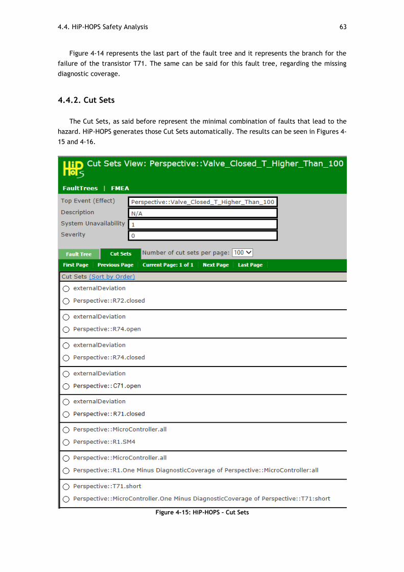
4.4. HiP-HOPS Safety Analysis 63
Figure 4-14 represents the last part of the fault tree and it represents the branch for the
failure of the transistor T71. The same can be said for this fault tree, regarding the missing
diagnostic coverage.
4.4.2. Cut Sets
The Cut Sets, as said before represent the minimal combination of faults that lead to the
hazard. HiP-HOPS generates those Cut Sets automatically. The results can be seen in Figures 4-
15 and 4-16.
Figure 4-15: HiP-HOPS – Cut Sets
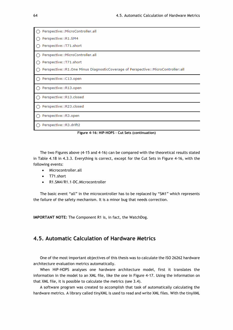
64 4.5. Automatic Calculation of Hardware Metrics
Figure 4-16: HiP-HOPS – Cut Sets (continuation)
The two Figures above (4-15 and 4-16) can be compared with the theoretical results stated
in Table 4.18 in 4.3.3. Everything is correct, except for the Cut Sets in Figure 4-16, with the
following events:
Microcontroller.all
T71.short
R1.SM4/R1.1-DC.Microcontroller
The basic event “all” in the microcontroller has to be replaced by “SM1” which represents
the failure of the safety mechanism. It is a minor bug that needs correction.
IMPORTANT NOTE: The Component R1 is, in fact, the WatchDog.
4.5. Automatic Calculation of Hardware Metrics
One of the most important objectives of this thesis was to calculate the ISO 26262 hardware
architecture evaluation metrics automatically.
When HiP-HOPS analyses one hardware architecture model, first it translates the
information in the model to an XML file, like the one in Figure 4-17. Using the information on
that XML file, it is possible to calculate the metrics (see 3.4).
A software program was created to accomplish that task of automatically calculating the
hardware metrics. A library called tinyXML is used to read and write XML files. With the tinyXML
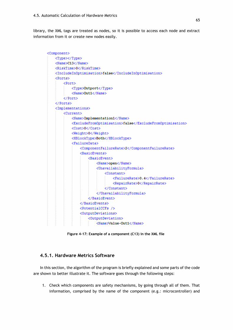
4.5. Automatic Calculation of Hardware Metrics 65
library, the XML tags are treated as nodes, so it is possible to access each node and extract
information from it or create new nodes easily.
Figure 4-17: Example of a component (C13) in the XML file
4.5.1. Hardware Metrics Software
In this section, the algorithm of the program is briefly explained and some parts of the code
are shown to better illustrate it. The software goes through the following steps:
1. Check which components are safety mechanisms, by going through all of them. That
information, comprised by the name of the component (e.g.: microcontroller) and
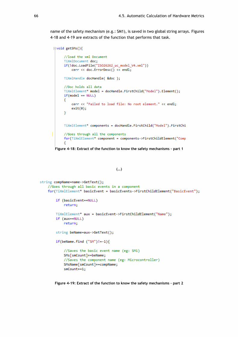
66 4.5. Automatic Calculation of Hardware Metrics
name of the safety mechanism (e.g.: SM1), is saved in two global string arrays. Figures
4-18 and 4-19 are extracts of the function that performs that task.
Figure 4-18: Extract of the function to know the safety mechanisms – part 1
(…)
Figure 4-19: Extract of the function to know the safety mechanisms – part 2
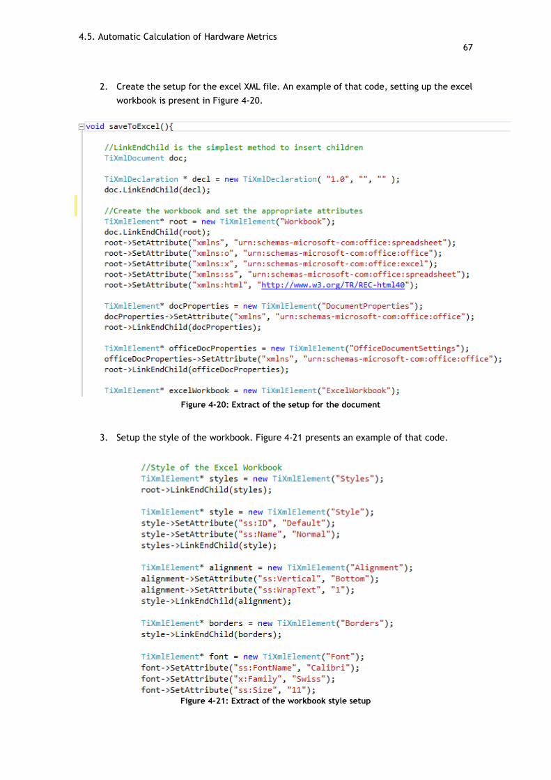
4.5. Automatic Calculation of Hardware Metrics 67
2. Create the setup for the excel XML file. An example of that code, setting up the excel
workbook is present in Figure 4-20.
3. Setup the style of the workbook. Figure 4-21 presents an example of that code.
Figure 4-21: Extract of the workbook style setup
Figure 4-20: Extract of the setup for the document
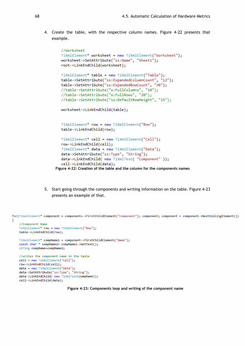
68 4.5. Automatic Calculation of Hardware Metrics
4. Create the table, with the respective column names. Figure 4-22 presents that
example.
Figure 4-22: Creation of the table and the column for the components names
5. Start going through the components and writing information on the table. Figure 4-23
presents an example of that.
Figure 4-23: Components loop and writing of the component name
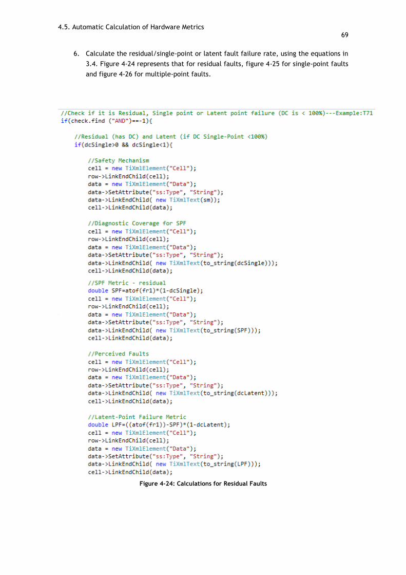
4.5. Automatic Calculation of Hardware Metrics 69
6. Calculate the residual/single-point or latent fault failure rate, using the equations in
3.4. Figure 4-24 represents that for residual faults, figure 4-25 for single-point faults
and figure 4-26 for multiple-point faults.
Figure 4-24: Calculations for Residual Faults
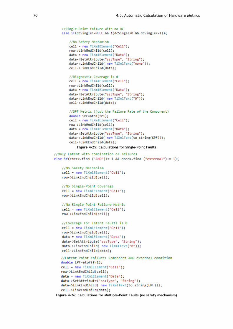
70 4.5. Automatic Calculation of Hardware Metrics
Figure 4-25: Calculations for Single-Point Faults
Figure 4-26: Calculations for Multiple-Point Faults (no safety mechanism)
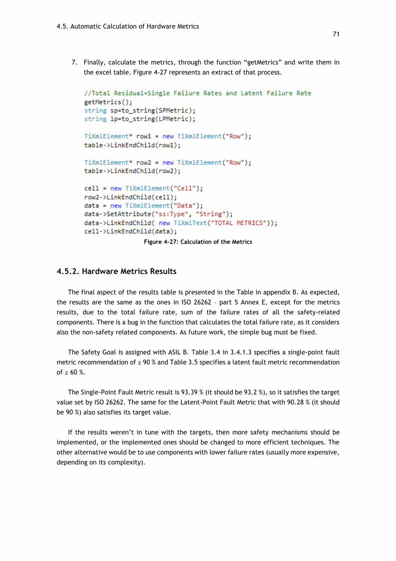
4.5. Automatic Calculation of Hardware Metrics 71
7. Finally, calculate the metrics, through the function “getMetrics” and write them in
the excel table. Figure 4-27 represents an extract of that process.
Figure 4-27: Calculation of the Metrics
4.5.2. Hardware Metrics Results
The final aspect of the results table is presented in the Table in appendix B. As expected,
the results are the same as the ones in ISO 26262 – part 5 Annex E, except for the metrics
results, due to the total failure rate, sum of the failure rates of all the safety-related
components. There is a bug in the function that calculates the total failure rate, as it considers
also the non-safety related components. As future work, the simple bug must be fixed.
The Safety Goal is assigned with ASIL B. Table 3.4 in 3.4.1.3 specifies a single-point fault
metric recommendation of ≥ 90 % and Table 3.5 specifies a latent fault metric recommendation
of ≥ 60 %.
The Single-Point Fault Metric result is 93.39 % (it should be 93.2 %), so it satisfies the target
value set by ISO 26262. The same for the Latent-Point Fault Metric that with 90.28 % (it should
be 90 %) also satisfies its target value.
If the results weren’t in tune with the targets, then more safety mechanisms should be
implemented, or the implemented ones should be changed to more efficient techniques. The
other alternative would be to use components with lower failure rates (usually more expensive,
depending on its complexity).
72 4.6. Summary
4.6. Summary
In this chapter, the chosen hardware architecture to validate the metrics results was
presented, and its operation explained. The failure propagation model of the chosen system
was outlined along with the failure annotations of the system’s components. Having the model,
it was possible to perform safety analysis. The fault tree for this system was manually created
in order to compare the results (fault tree and cut-sets) with the HiP-HOPS analysis. The latter
was changed to include safety mechanisms. Finally, the algorithm of the program created to
automatically calculate the hardware evaluation metrics is explained.

4.6. Summary 73
74 5.1. Final Considerations
Chapter 5
Conclusion
The vehicles developed in the near future, will have most of their critical functions, such
as steering and braking, controlled by systems containing electrical, electronic and
programmable electronic components. Not to mention cars that integrate hybrid technologies.
These changes are being implemented to increase the vehicle’s commodities and safety and
decrease fuel consumption through a more adequate driving behavior. To assure that those
systems are the most reliable they can be, Functional Safety Standards, such as IEC 61508 or
ISO 26262 (specially created for road vehicles) aid the developers with guidelines for their
development. One important measure to guarantee the reliability of these systems is to add
safety mechanisms. These detect failures in the systems and activate measures that control
them and avoid safety goal violation.
As this type of systems, suffer changes throughout the development process, it is important
to test those changes during that process and not only in the beginning or when system failures
occur. With that in mind, Safety Analysis tools, like HiP-HOPS were created.
In this thesis, safety mechanisms were included in the HiP-HOPS analysis, by changing the
code. Also, a C++ software program (Appendix C) was developed to automatically calculate the
hardware evaluation metrics, proposed in ISO 26262. These metrics allow the system designer
to compare different system architectures.
The relevance of the work developed is be discussed in the next sections and the final
considerations about it are presented. To finalize, possible future changes to HiP-HOPS,
regarding hardware evaluation and developments to the software program are presented.
5.1. Final Considerations
The results achieved in the Safety Analysis done through HiP-HOPS namely the Fault Trees
and Cut Sets, comply with the ideas stated in ISO 26262 in regard to safety mechanism
modelling. Furthermore, the Fault Trees produced by HiP-HOPS are now capable of dealing with
the probabilistic metric (PMHF).
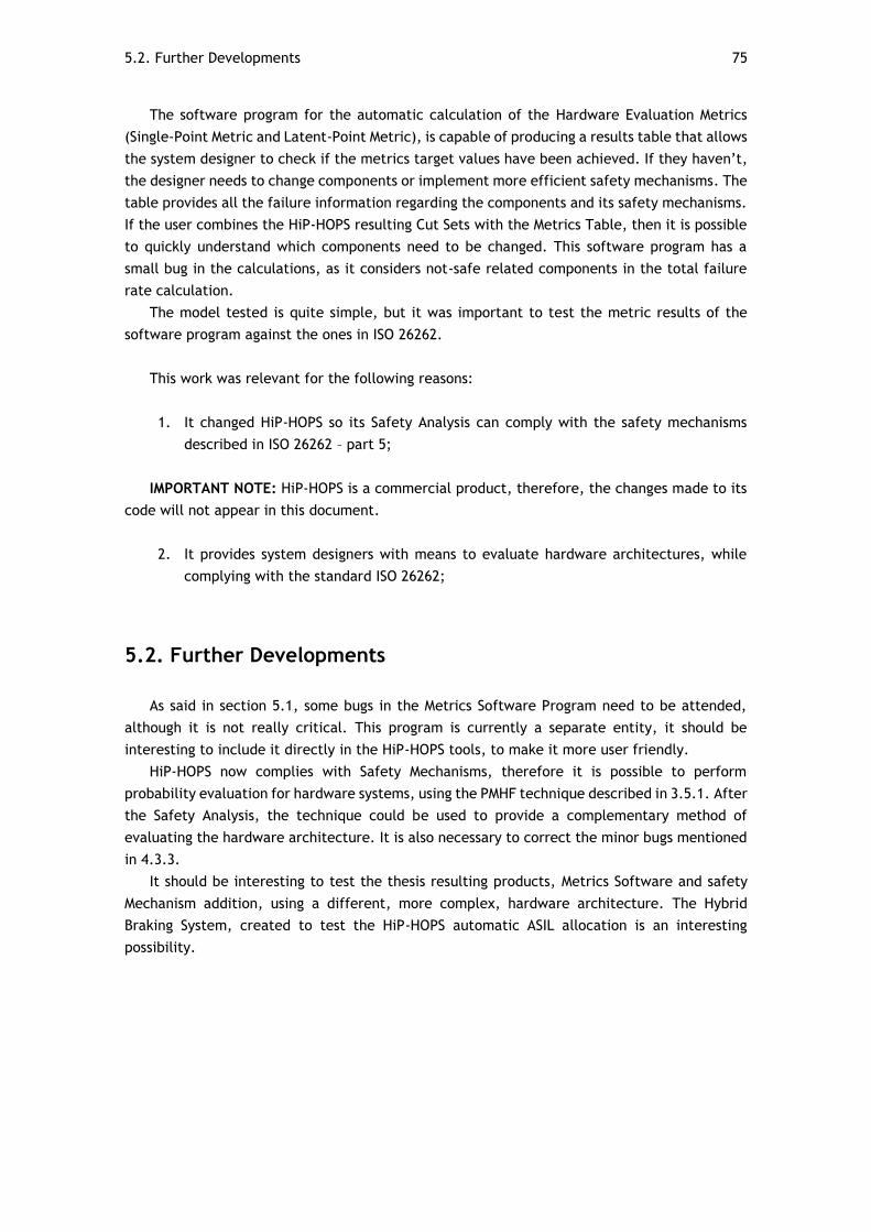
5.2. Further Developments 75
The software program for the automatic calculation of the Hardware Evaluation Metrics
(Single-Point Metric and Latent-Point Metric), is capable of producing a results table that allows
the system designer to check if the metrics target values have been achieved. If they haven’t,
the designer needs to change components or implement more efficient safety mechanisms. The
table provides all the failure information regarding the components and its safety mechanisms.
If the user combines the HiP-HOPS resulting Cut Sets with the Metrics Table, then it is possible
to quickly understand which components need to be changed. This software program has a
small bug in the calculations, as it considers not-safe related components in the total failure
rate calculation.
The model tested is quite simple, but it was important to test the metric results of the
software program against the ones in ISO 26262.
This work was relevant for the following reasons:
1. It changed HiP-HOPS so its Safety Analysis can comply with the safety mechanisms
described in ISO 26262 – part 5;
IMPORTANT NOTE: HiP-HOPS is a commercial product, therefore, the changes made to its
code will not appear in this document.
2. It provides system designers with means to evaluate hardware architectures, while
complying with the standard ISO 26262;
5.2. Further Developments
As said in section 5.1, some bugs in the Metrics Software Program need to be attended,
although it is not really critical. This program is currently a separate entity, it should be
interesting to include it directly in the HiP-HOPS tools, to make it more user friendly.
HiP-HOPS now complies with Safety Mechanisms, therefore it is possible to perform
probability evaluation for hardware systems, using the PMHF technique described in 3.5.1. After
the Safety Analysis, the technique could be used to provide a complementary method of
evaluating the hardware architecture. It is also necessary to correct the minor bugs mentioned
in 4.3.3.
It should be interesting to test the thesis resulting products, Metrics Software and safety
Mechanism addition, using a different, more complex, hardware architecture. The Hybrid
Braking System, created to test the HiP-HOPS automatic ASIL allocation is an interesting
possibility.

76 5.2. Further Developments
5.2. Further Developments 77
References
[1] ISO 26262-1, Road vehicles — Functional safety, First Edition, 2011-11-15
[2] HiP-HOPS User Manual, version 2.5, July 2013
[3] Adachi, M., Papadopoulos, Y., Sharvia, S., Parker and D., Tohdo, T. (2011). "An approach to
optimization of fault tolerant architectures using HiP-HOPS." Software - Practice and
Experience 41(11): 1303-1327.
[4] Mahmud, N., Papadopoulos, Y. and Walker, M. (2010). “A translation of state machines to
temporal fault trees.” Department of Computer Science, University of Hull.
[5] Nggada, S. H., Parker, D. J. and Papadopoulos, Y. I. (2010). “Dynamic effect of perfect
preventive maintenance on system reliability and cost using HiP-HOPS.” Department of
Computer Science, University of Hull.
[6] Papadopoulos, Y., Walker, M., Parker, D., Rüde, E., Hamann, R., Uhlig, A., Grätz, U. and
Lien, R. (2011). "Engineering failure analysis and design optimization with HiP-HOPS."
Engineering Failure Analysis 18(2): 590-608.
[7] Papadopoulos, Y., Walker, M., Reiser, M-O, Weber, M., Chen, D., Törngren, M., Servat, D.,
Abele, A., Stappert, F., Lonn, H., Berntsson, L., Johansson, R., Tagliabo, F., Torchiaro, S. and
Sandberg, A. (2010). “Automatic allocation of safety integrity levels.” CARS’, April 27,
Valencia, Spain.
[8] Sharvia, S. and Y. Papadopoulos (2011). “Integrated application of compositional and
behavioural safety analysis.” Advances in Intelligent and Soft Computing 97: 179-192.
[9] Wolforth, I., Walker, M., Papadopoulos, Y. and Grunske, L. (2010). "Capture and reuse of
composable failure patterns." International Journal of Critical Computer-Based Systems 1(1-3):
128-147.
[10] Rupanov, V., Knoll, A., Fiege, L., Armbruster, M., Spiegelberg, G. and Buckl, C. (2012).
“Early Safety Evaluation of Design Decisions in E/E Architecture according to ISO 26262.”
ISARCS'12. Bertinoro, Italy.
[11] M. Walker and Y. Papadopoulos, "PANDORA: The time of Priority AND gates," in INCOM
2006, 12th IFAC Int’l Symposium on Information Control Problems in Manufacturing,
France, 2006, pp. 235-240. [12] Sinha, P. (2011). "Architectural design and reliability analysis of a fail-operational brake-by-wire system from ISO 26262 perspectives." Reliability Engineering and System Safety.
[13] Hillenbrand, M., Heinz, M., Adler, N., Matheis, J. and Müller-Glaser, K. D. (2010). "Failure
mode and effect analysis based on electric and electronic architectures of vehicles to support
the safety lifecycle ISO/DIS 26262." [14] Jeon, S.-H., Cho, J.-H-, Jung, Y., Park, S. and Han, T.-M. (2011). "Automotive Hardware Development According to ISO 26262." ICACT 2011

78 5.2. Further Developments
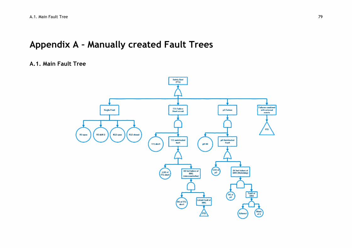
A.1. Main Fault Tree 79
Appendix A – Manually created Fault Trees
A.1. Main Fault Tree
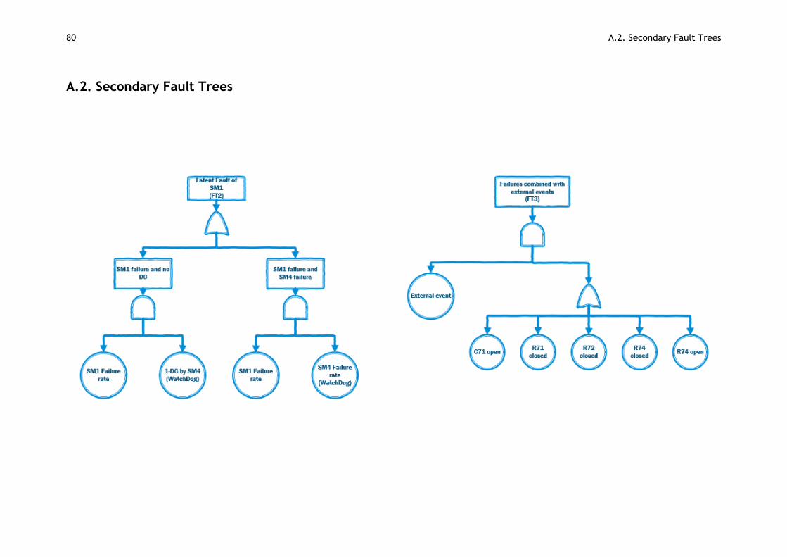
80 A.2. Secondary Fault Trees
A.2. Secondary Fault Trees
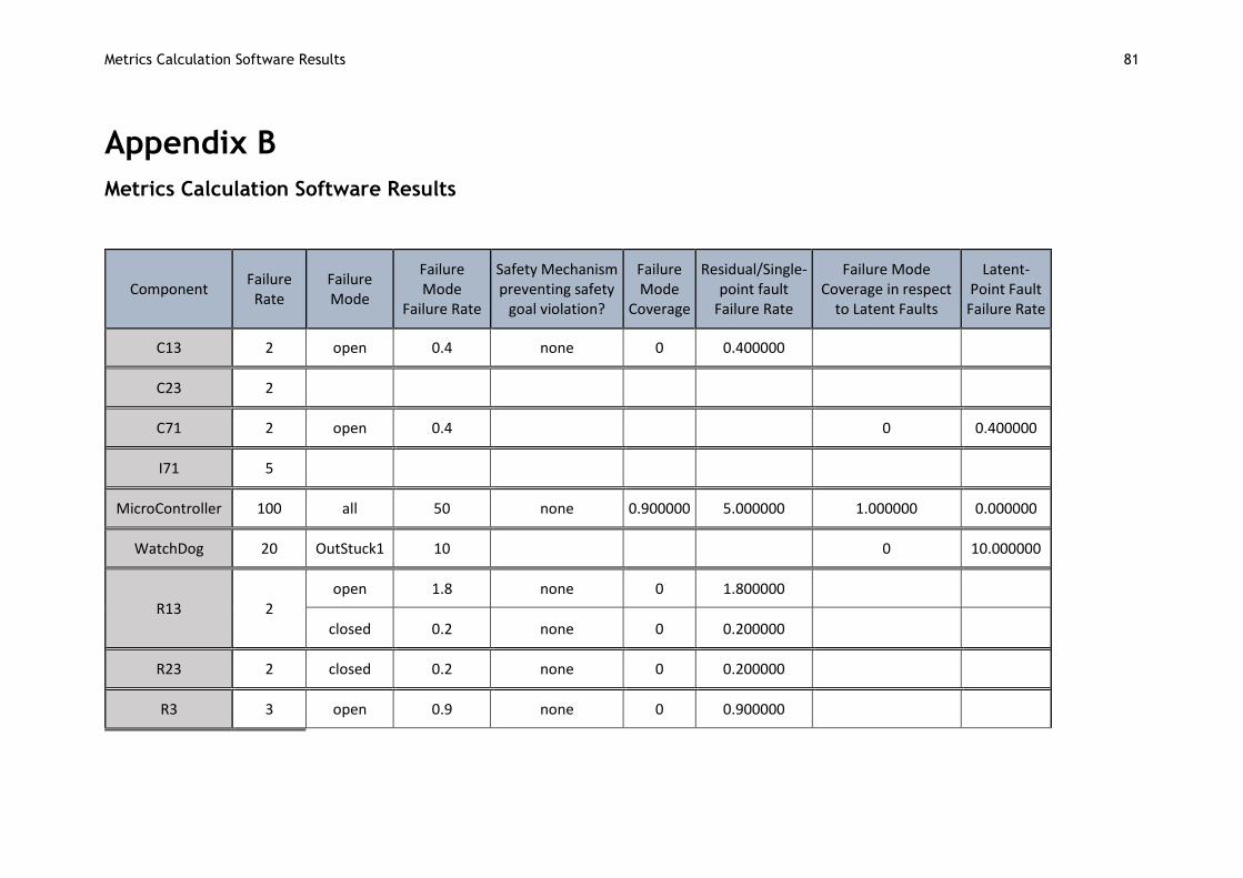
Metrics Calculation Software Results 81
Appendix B
Metrics Calculation Software Results
Component Failure
Rate Failure Mode
Failure Mode
Failure Rate
Safety Mechanism preventing safety
goal violation?
Failure Mode
Coverage
Residual/Single-point fault
Failure Rate
Failure Mode Coverage in respect
to Latent Faults
Latent-Point Fault
Failure Rate
C13 2 open 0.4 none 0 0.400000
C23 2
C71 2 open 0.4 0 0.400000
I71 5
MicroController 100 all 50 none 0.900000 5.000000 1.000000 0.000000
WatchDog 20 OutStuck1 10 0 10.000000
R13 2 open 1.8 none 0 1.800000
closed 0.2 none 0 0.200000
R23 2 closed 0.2 none 0 0.200000
R3 3 open 0.9 none 0 0.900000
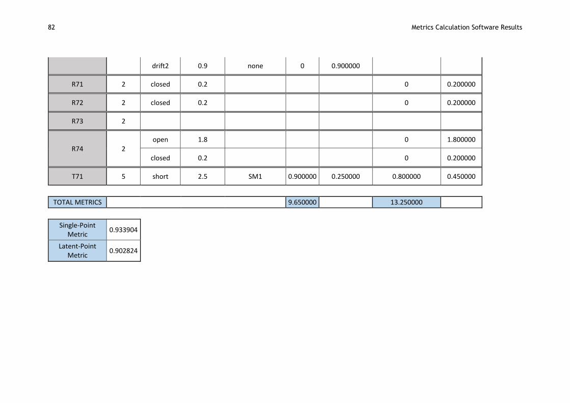
82 Metrics Calculation Software Results
drift2 0.9 none 0 0.900000
R71 2 closed 0.2 0 0.200000
R72 2 closed 0.2 0 0.200000
R73 2
R74 2 open 1.8 0 1.800000
closed 0.2 0 0.200000
T71 5 short 2.5 SM1 0.900000 0.250000 0.800000 0.450000
TOTAL METRICS 9.650000 13.250000
Single-Point Metric
0.933904
Latent-Point Metric
0.902824

Metrics Software 83
Appendix C
Metrics Software
This appendix contains the whole code of the Metrics Calculation Software.
#include <stdio.h> #include <iostream> #include "tinyxml.h" #include "string.h" #include <vector> #include <fstream> using namespace std; double totalFailureRate; bool isSPF; bool isLPF; double SPMetric; double LPMetric; string SMs[20]; int smCount; string SMsName[20]; void GetTotalFailureRate(){ //load the xml Document TiXmlDocument doc; if(!doc.LoadFile("ISO26262_uc_model_V4.xml")) cerr << doc.ErrorDesc() << endl;
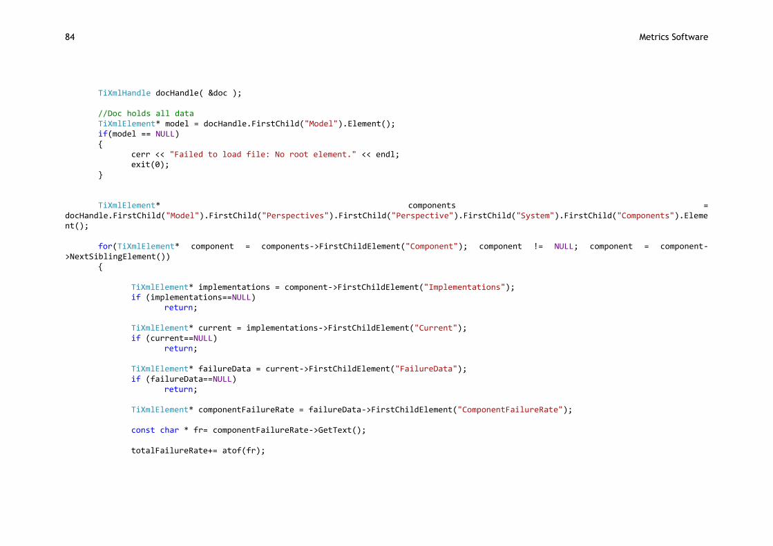
84 Metrics Software
TiXmlHandle docHandle( &doc ); //Doc holds all data TiXmlElement* model = docHandle.FirstChild("Model").Element(); if(model == NULL) { cerr << "Failed to load file: No root element." << endl; exit(0); } TiXmlElement* components = docHandle.FirstChild("Model").FirstChild("Perspectives").FirstChild("Perspective").FirstChild("System").FirstChild("Components").Element(); for(TiXmlElement* component = components->FirstChildElement("Component"); component != NULL; component = component->NextSiblingElement()) { TiXmlElement* implementations = component->FirstChildElement("Implementations"); if (implementations==NULL) return; TiXmlElement* current = implementations->FirstChildElement("Current"); if (current==NULL) return; TiXmlElement* failureData = current->FirstChildElement("FailureData"); if (failureData==NULL) return; TiXmlElement* componentFailureRate = failureData->FirstChildElement("ComponentFailureRate"); const char * fr= componentFailureRate->GetText(); totalFailureRate+= atof(fr);
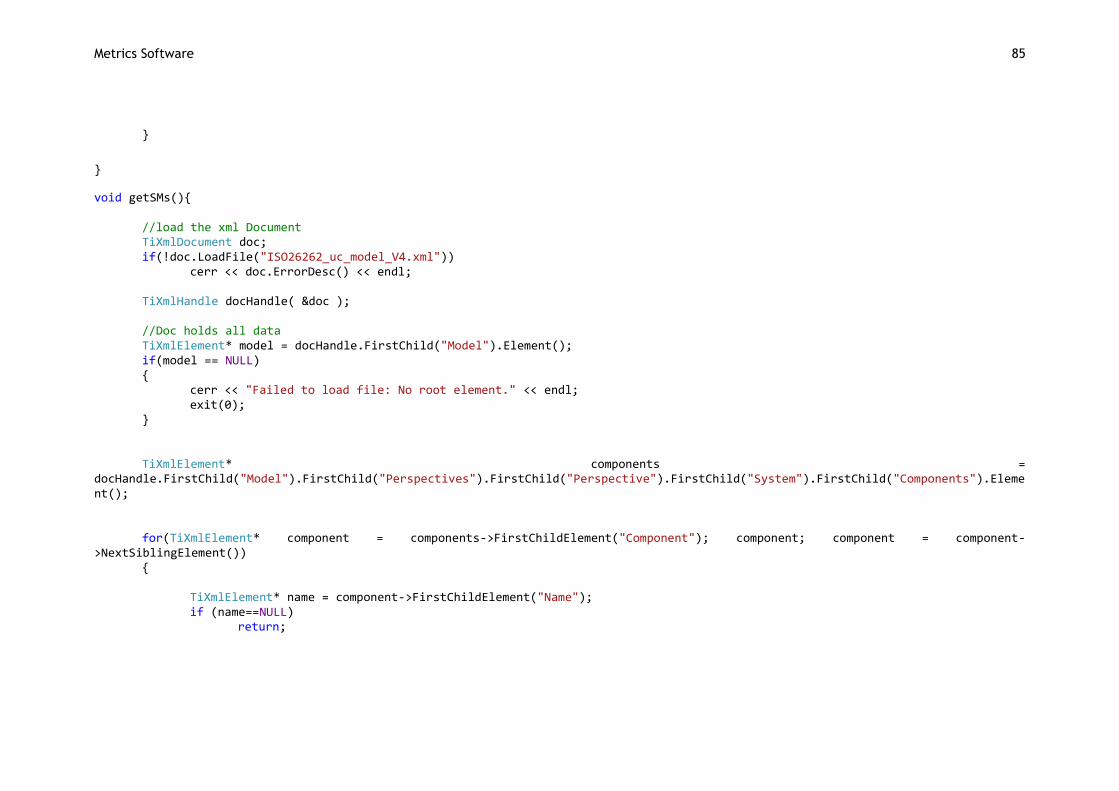
Metrics Software 85
}
}
void getSMs(){ //load the xml Document TiXmlDocument doc; if(!doc.LoadFile("ISO26262_uc_model_V4.xml")) cerr << doc.ErrorDesc() << endl; TiXmlHandle docHandle( &doc ); //Doc holds all data TiXmlElement* model = docHandle.FirstChild("Model").Element(); if(model == NULL) { cerr << "Failed to load file: No root element." << endl; exit(0); } TiXmlElement* components = docHandle.FirstChild("Model").FirstChild("Perspectives").FirstChild("Perspective").FirstChild("System").FirstChild("Components").Element(); for(TiXmlElement* component = components->FirstChildElement("Component"); component; component = component->NextSiblingElement()) { TiXmlElement* name = component->FirstChildElement("Name"); if (name==NULL) return;
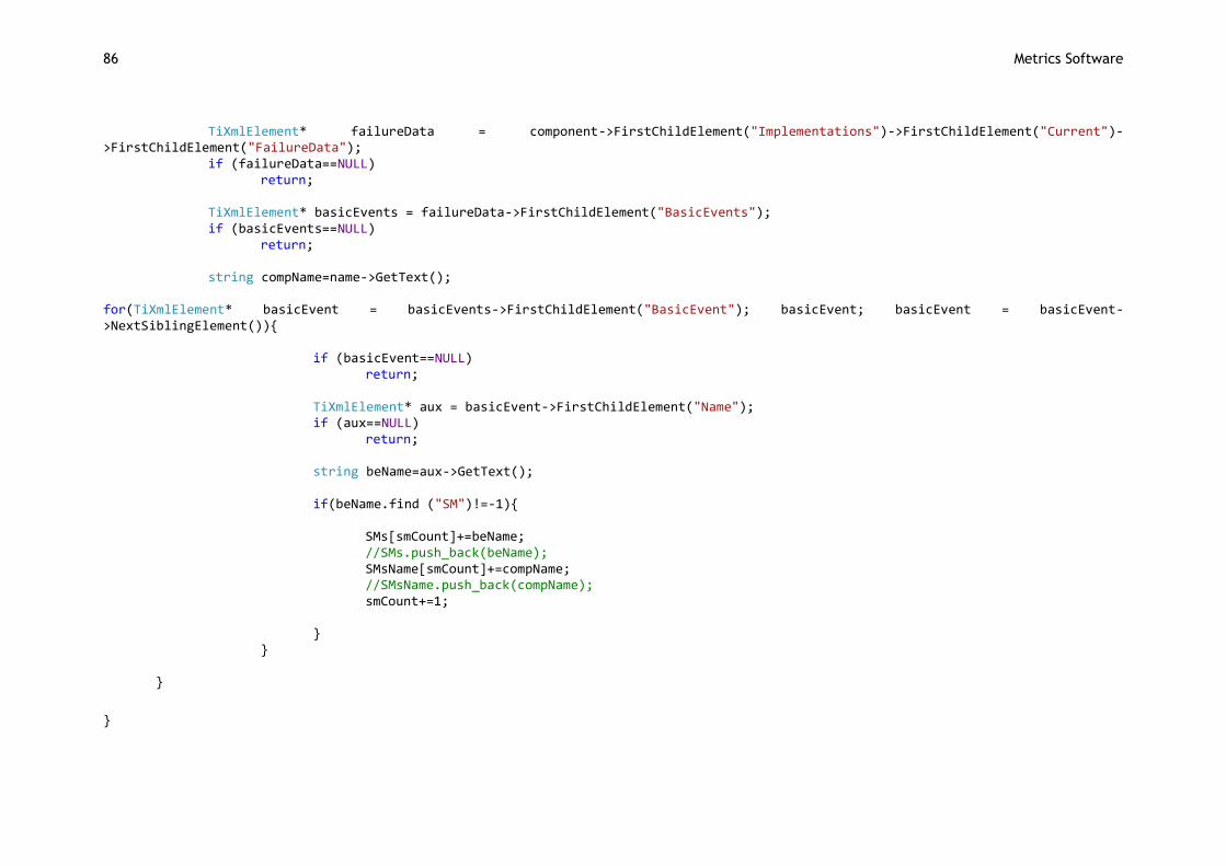
86 Metrics Software
TiXmlElement* failureData = component->FirstChildElement("Implementations")->FirstChildElement("Current")->FirstChildElement("FailureData"); if (failureData==NULL) return; TiXmlElement* basicEvents = failureData->FirstChildElement("BasicEvents"); if (basicEvents==NULL) return; string compName=name->GetText(); for(TiXmlElement* basicEvent = basicEvents->FirstChildElement("BasicEvent"); basicEvent; basicEvent = basicEvent->NextSiblingElement()){ if (basicEvent==NULL) return; TiXmlElement* aux = basicEvent->FirstChildElement("Name"); if (aux==NULL) return; string beName=aux->GetText(); if(beName.find ("SM")!=-1){ SMs[smCount]+=beName; //SMs.push_back(beName); SMsName[smCount]+=compName; //SMsName.push_back(compName); smCount+=1; } } }
}
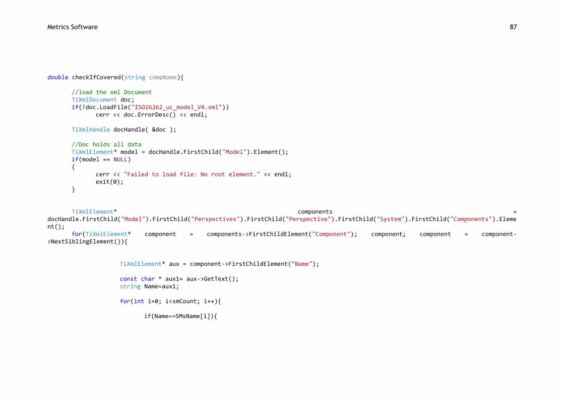
Metrics Software 87
double checkIfCovered(string compName){ //load the xml Document TiXmlDocument doc; if(!doc.LoadFile("ISO26262_uc_model_V4.xml")) cerr << doc.ErrorDesc() << endl; TiXmlHandle docHandle( &doc ); //Doc holds all data TiXmlElement* model = docHandle.FirstChild("Model").Element(); if(model == NULL) { cerr << "Failed to load file: No root element." << endl; exit(0); } TiXmlElement* components = docHandle.FirstChild("Model").FirstChild("Perspectives").FirstChild("Perspective").FirstChild("System").FirstChild("Components").Element(); for(TiXmlElement* component = components->FirstChildElement("Component"); component; component = component->NextSiblingElement()){ TiXmlElement* aux = component->FirstChildElement("Name"); const char * aux1= aux->GetText(); string Name=aux1; for(int i=0; i<smCount; i++){ if(Name==SMsName[i]){
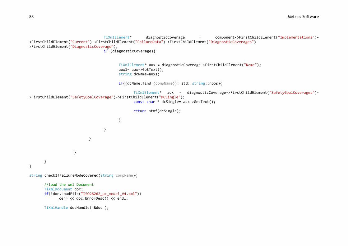
88 Metrics Software
TiXmlElement* diagnosticCoverage = component->FirstChildElement("Implementations")->FirstChildElement("Current")->FirstChildElement("FailureData")->FirstChildElement("DiagnosticCoverages")->FirstChildElement("DiagnosticCoverage"); if (diagnosticCoverage){ TiXmlElement* aux = diagnosticCoverage->FirstChildElement("Name"); aux1= aux->GetText(); string dcName=aux1; if((dcName.find (compName))!=std::string::npos){ TiXmlElement* aux = diagnosticCoverage->FirstChildElement("SafetyGoalCoverages")->FirstChildElement("SafetyGoalCoverage")->FirstChildElement("DCSingle"); const char * dcSingle= aux->GetText(); return atof(dcSingle); } } } } } } string checkIfFailureModeCovered(string compName){ //load the xml Document TiXmlDocument doc; if(!doc.LoadFile("ISO26262_uc_model_V4.xml")) cerr << doc.ErrorDesc() << endl; TiXmlHandle docHandle( &doc );
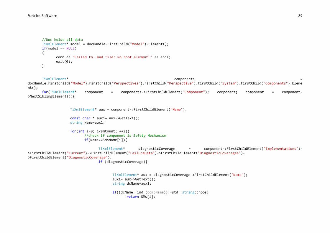
Metrics Software 89
//Doc holds all data TiXmlElement* model = docHandle.FirstChild("Model").Element(); if(model == NULL) { cerr << "Failed to load file: No root element." << endl; exit(0); } TiXmlElement* components = docHandle.FirstChild("Model").FirstChild("Perspectives").FirstChild("Perspective").FirstChild("System").FirstChild("Components").Element(); for(TiXmlElement* component = components->FirstChildElement("Component"); component; component = component->NextSiblingElement()){ TiXmlElement* aux = component->FirstChildElement("Name"); const char * aux1= aux->GetText(); string Name=aux1; for(int i=0; i<smCount; ++i){ //check if component is Safety Mechanism if(Name==SMsName[i]){ TiXmlElement* diagnosticCoverage = component->FirstChildElement("Implementations")->FirstChildElement("Current")->FirstChildElement("FailureData")->FirstChildElement("DiagnosticCoverages")->FirstChildElement("DiagnosticCoverage"); if (diagnosticCoverage){ TiXmlElement* aux = diagnosticCoverage->FirstChildElement("Name"); aux1= aux->GetText(); string dcName=aux1; if((dcName.find (compName))!=std::string::npos) return SMs[i];
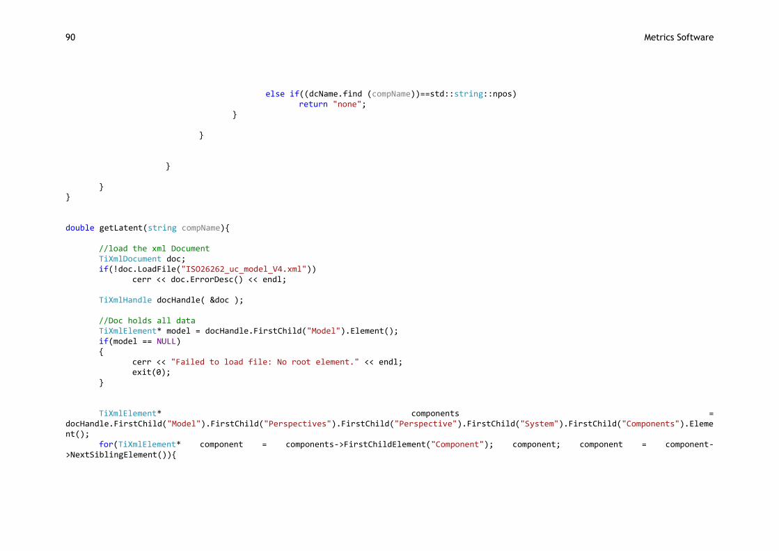
90 Metrics Software
else if((dcName.find (compName))==std::string::npos) return "none"; } } } } } double getLatent(string compName){ //load the xml Document TiXmlDocument doc; if(!doc.LoadFile("ISO26262_uc_model_V4.xml")) cerr << doc.ErrorDesc() << endl; TiXmlHandle docHandle( &doc ); //Doc holds all data TiXmlElement* model = docHandle.FirstChild("Model").Element(); if(model == NULL) { cerr << "Failed to load file: No root element." << endl; exit(0); } TiXmlElement* components = docHandle.FirstChild("Model").FirstChild("Perspectives").FirstChild("Perspective").FirstChild("System").FirstChild("Components").Element(); for(TiXmlElement* component = components->FirstChildElement("Component"); component; component = component->NextSiblingElement()){
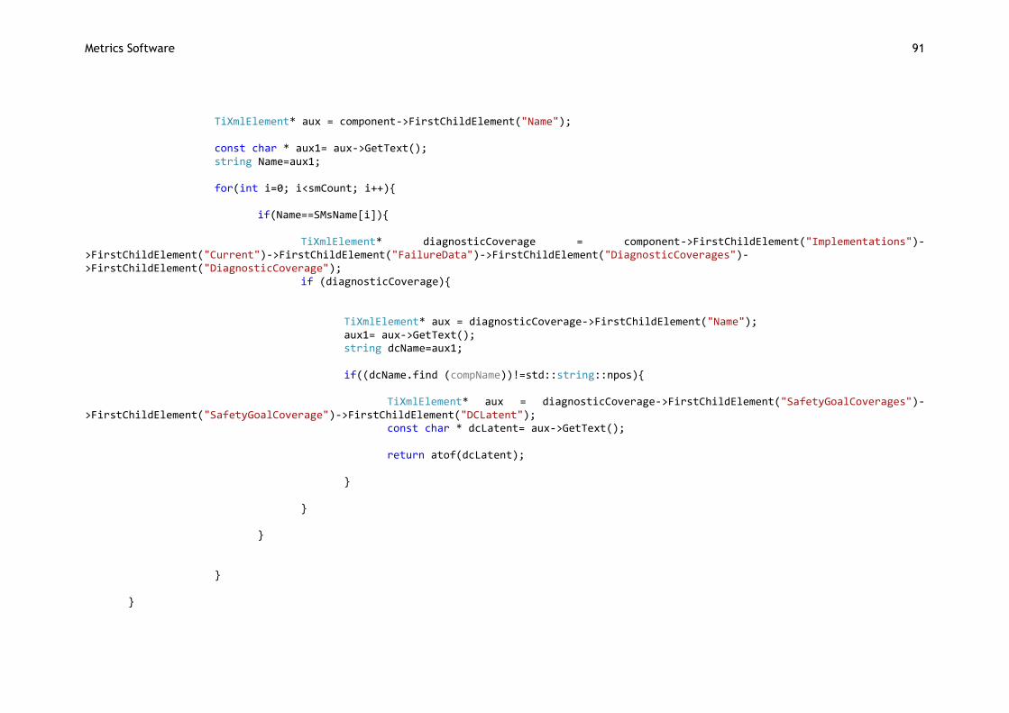
Metrics Software 91
TiXmlElement* aux = component->FirstChildElement("Name"); const char * aux1= aux->GetText(); string Name=aux1; for(int i=0; i<smCount; i++){ if(Name==SMsName[i]){ TiXmlElement* diagnosticCoverage = component->FirstChildElement("Implementations")->FirstChildElement("Current")->FirstChildElement("FailureData")->FirstChildElement("DiagnosticCoverages")->FirstChildElement("DiagnosticCoverage"); if (diagnosticCoverage){ TiXmlElement* aux = diagnosticCoverage->FirstChildElement("Name"); aux1= aux->GetText(); string dcName=aux1; if((dcName.find (compName))!=std::string::npos){ TiXmlElement* aux = diagnosticCoverage->FirstChildElement("SafetyGoalCoverages")->FirstChildElement("SafetyGoalCoverage")->FirstChildElement("DCLatent"); const char * dcLatent= aux->GetText(); return atof(dcLatent); } } } } }
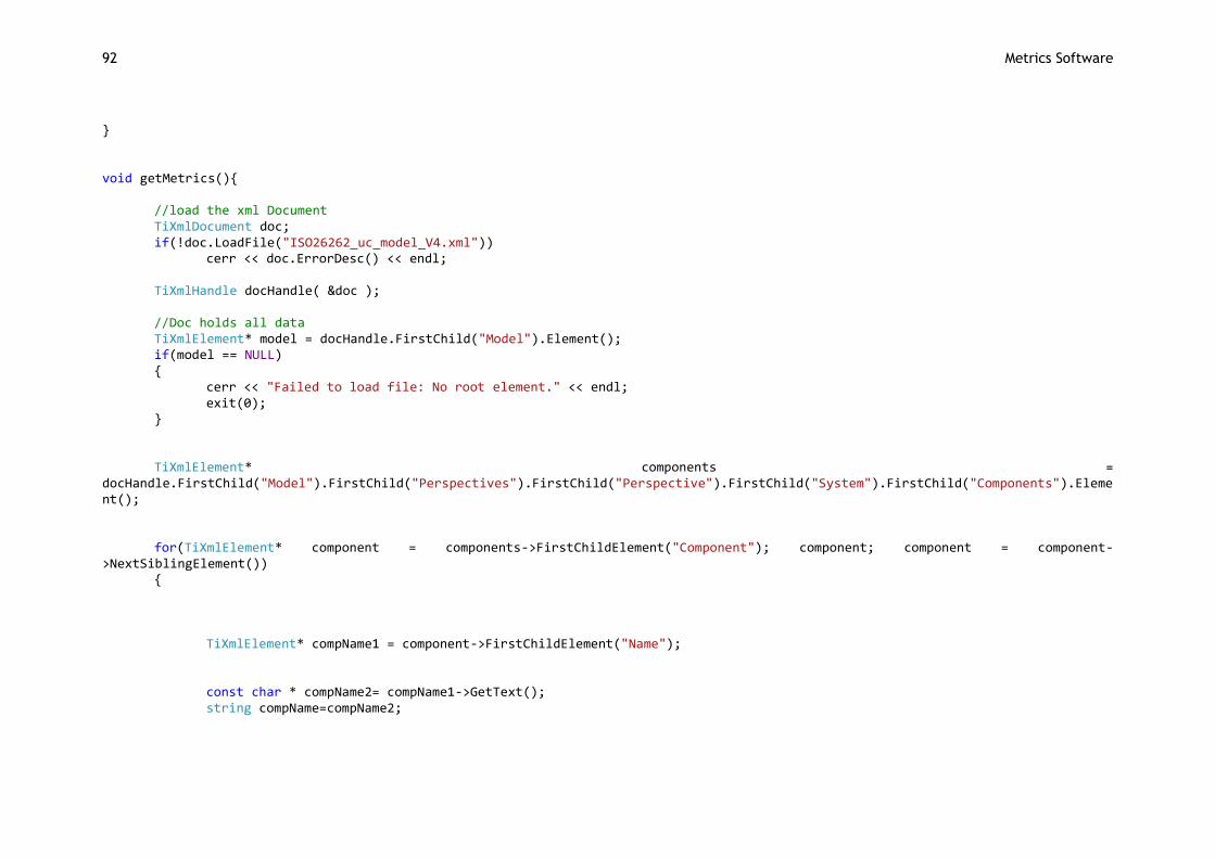
92 Metrics Software
} void getMetrics(){ //load the xml Document TiXmlDocument doc; if(!doc.LoadFile("ISO26262_uc_model_V4.xml")) cerr << doc.ErrorDesc() << endl; TiXmlHandle docHandle( &doc ); //Doc holds all data TiXmlElement* model = docHandle.FirstChild("Model").Element(); if(model == NULL) { cerr << "Failed to load file: No root element." << endl; exit(0); } TiXmlElement* components = docHandle.FirstChild("Model").FirstChild("Perspectives").FirstChild("Perspective").FirstChild("System").FirstChild("Components").Element(); for(TiXmlElement* component = components->FirstChildElement("Component"); component; component = component->NextSiblingElement()) { TiXmlElement* compName1 = component->FirstChildElement("Name"); const char * compName2= compName1->GetText(); string compName=compName2;
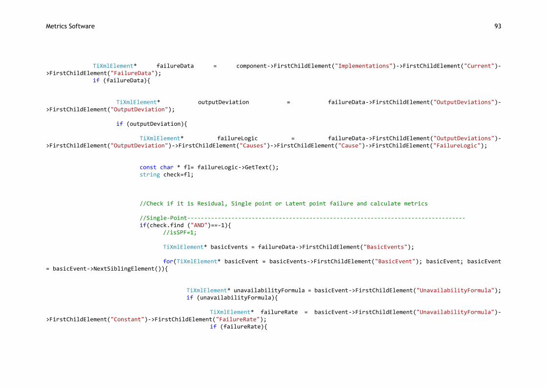
Metrics Software 93
TiXmlElement* failureData = component->FirstChildElement("Implementations")->FirstChildElement("Current")->FirstChildElement("FailureData"); if (failureData){ TiXmlElement* outputDeviation = failureData->FirstChildElement("OutputDeviations")->FirstChildElement("OutputDeviation"); if (outputDeviation){ TiXmlElement* failureLogic = failureData->FirstChildElement("OutputDeviations")->FirstChildElement("OutputDeviation")->FirstChildElement("Causes")->FirstChildElement("Cause")->FirstChildElement("FailureLogic"); const char * fl= failureLogic->GetText(); string check=fl; //Check if it is Residual, Single point or Latent point failure and calculate metrics //Single-Point---------------------------------------------------------------------------------- if(check.find ("AND")==-1){ //isSPF=1; TiXmlElement* basicEvents = failureData->FirstChildElement("BasicEvents"); for(TiXmlElement* basicEvent = basicEvents->FirstChildElement("BasicEvent"); basicEvent; basicEvent = basicEvent->NextSiblingElement()){ TiXmlElement* unavailabilityFormula = basicEvent->FirstChildElement("UnavailabilityFormula"); if (unavailabilityFormula){ TiXmlElement* failureRate = basicEvent->FirstChildElement("UnavailabilityFormula")->FirstChildElement("Constant")->FirstChildElement("FailureRate"); if (failureRate){

94 Metrics Software
const char * fr= failureRate->GetText(); double dcSingle=checkIfCovered(compName); if(dcSingle>0 && dcSingle<1) { SPMetric+= atof(fr) * (1-dcSingle); //Latent for Residual double dcLatent=getLatent(compName); double n= atof(fr) * (1-dcSingle); LPMetric+= ((atof(fr))-n)*(1-dcLatent); } else if(dcSingle!=NULL && !(dcSingle>0 && dcSingle<=1)) SPMetric+= atof(fr); } } } } //Latent -------------------------------------------------------------------------------- else if(check.find ("AND")!=-1 && check.find ("external")!=-1){ //isSPF=1; TiXmlElement* basicEvents = failureData->FirstChildElement("BasicEvents"); for(TiXmlElement* basicEvent = basicEvents->FirstChildElement("BasicEvent"); basicEvent; basicEvent = basicEvent->NextSiblingElement()){ TiXmlElement* aux = basicEvent->FirstChildElement("Name");
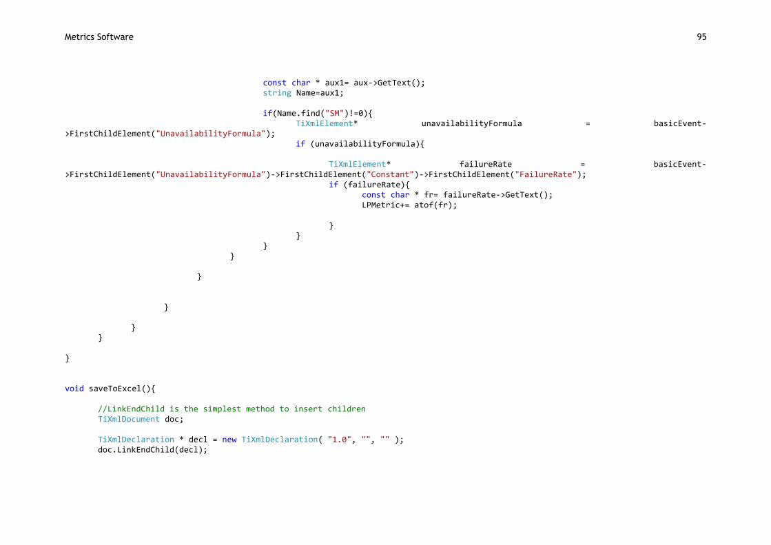
Metrics Software 95
const char * aux1= aux->GetText(); string Name=aux1; if(Name.find("SM")!=0){ TiXmlElement* unavailabilityFormula = basicEvent->FirstChildElement("UnavailabilityFormula"); if (unavailabilityFormula){ TiXmlElement* failureRate = basicEvent->FirstChildElement("UnavailabilityFormula")->FirstChildElement("Constant")->FirstChildElement("FailureRate"); if (failureRate){ const char * fr= failureRate->GetText(); LPMetric+= atof(fr); } } } } } } } } } void saveToExcel(){ //LinkEndChild is the simplest method to insert children TiXmlDocument doc; TiXmlDeclaration * decl = new TiXmlDeclaration( "1.0", "", "" ); doc.LinkEndChild(decl);
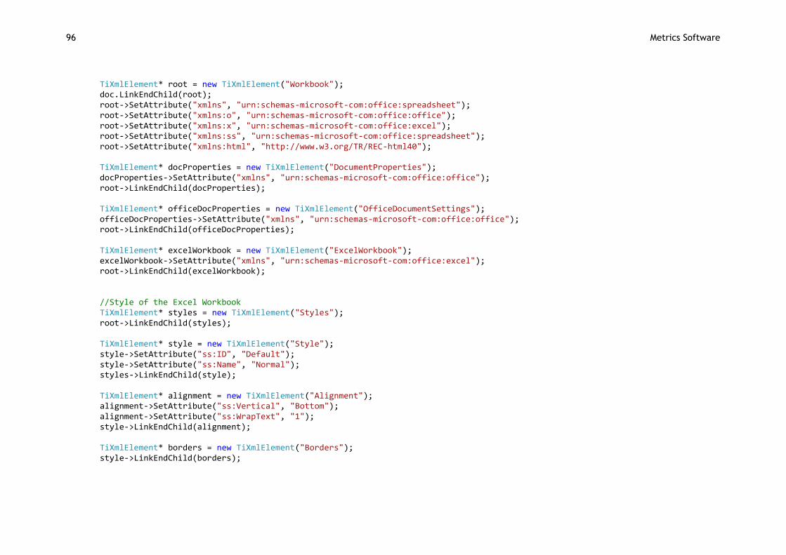
96 Metrics Software
TiXmlElement* root = new TiXmlElement("Workbook"); doc.LinkEndChild(root); root->SetAttribute("xmlns", "urn:schemas-microsoft-com:office:spreadsheet"); root->SetAttribute("xmlns:o", "urn:schemas-microsoft-com:office:office"); root->SetAttribute("xmlns:x", "urn:schemas-microsoft-com:office:excel"); root->SetAttribute("xmlns:ss", "urn:schemas-microsoft-com:office:spreadsheet"); root->SetAttribute("xmlns:html", "http://www.w3.org/TR/REC-html40"); TiXmlElement* docProperties = new TiXmlElement("DocumentProperties"); docProperties->SetAttribute("xmlns", "urn:schemas-microsoft-com:office:office"); root->LinkEndChild(docProperties); TiXmlElement* officeDocProperties = new TiXmlElement("OfficeDocumentSettings"); officeDocProperties->SetAttribute("xmlns", "urn:schemas-microsoft-com:office:office"); root->LinkEndChild(officeDocProperties); TiXmlElement* excelWorkbook = new TiXmlElement("ExcelWorkbook"); excelWorkbook->SetAttribute("xmlns", "urn:schemas-microsoft-com:office:excel"); root->LinkEndChild(excelWorkbook); //Style of the Excel Workbook TiXmlElement* styles = new TiXmlElement("Styles"); root->LinkEndChild(styles); TiXmlElement* style = new TiXmlElement("Style"); style->SetAttribute("ss:ID", "Default"); style->SetAttribute("ss:Name", "Normal"); styles->LinkEndChild(style); TiXmlElement* alignment = new TiXmlElement("Alignment"); alignment->SetAttribute("ss:Vertical", "Bottom"); alignment->SetAttribute("ss:WrapText", "1"); style->LinkEndChild(alignment); TiXmlElement* borders = new TiXmlElement("Borders"); style->LinkEndChild(borders);
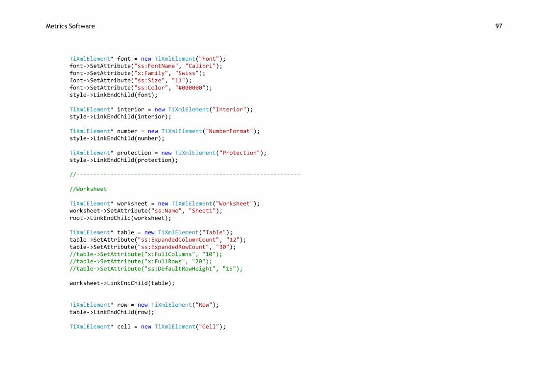
Metrics Software 97
TiXmlElement* font = new TiXmlElement("Font"); font->SetAttribute("ss:FontName", "Calibri"); font->SetAttribute("x:Family", "Swiss"); font->SetAttribute("ss:Size", "11"); font->SetAttribute("ss:Color", "#000000"); style->LinkEndChild(font); TiXmlElement* interior = new TiXmlElement("Interior"); style->LinkEndChild(interior); TiXmlElement* number = new TiXmlElement("NumberFormat"); style->LinkEndChild(number); TiXmlElement* protection = new TiXmlElement("Protection"); style->LinkEndChild(protection); //------------------------------------------------------------------ //Worksheet TiXmlElement* worksheet = new TiXmlElement("Worksheet"); worksheet->SetAttribute("ss:Name", "Sheet1"); root->LinkEndChild(worksheet); TiXmlElement* table = new TiXmlElement("Table"); table->SetAttribute("ss:ExpandedColumnCount", "12"); table->SetAttribute("ss:ExpandedRowCount", "30"); //table->SetAttribute("x:FullColumns", "10"); //table->SetAttribute("x:FullRows", "20"); //table->SetAttribute("ss:DefaultRowHeight", "15"); worksheet->LinkEndChild(table); TiXmlElement* row = new TiXmlElement("Row"); table->LinkEndChild(row); TiXmlElement* cell = new TiXmlElement("Cell");
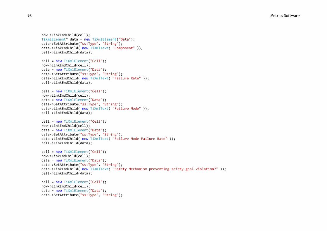
98 Metrics Software
row->LinkEndChild(cell); TiXmlElement* data = new TiXmlElement("Data"); data->SetAttribute("ss:Type", "String"); data->LinkEndChild( new TiXmlText( "Component" )); cell->LinkEndChild(data); cell = new TiXmlElement("Cell"); row->LinkEndChild(cell); data = new TiXmlElement("Data"); data->SetAttribute("ss:Type", "String"); data->LinkEndChild( new TiXmlText( "Failure Rate" )); cell->LinkEndChild(data); cell = new TiXmlElement("Cell"); row->LinkEndChild(cell); data = new TiXmlElement("Data"); data->SetAttribute("ss:Type", "String"); data->LinkEndChild( new TiXmlText( "Failure Mode" )); cell->LinkEndChild(data); cell = new TiXmlElement("Cell"); row->LinkEndChild(cell); data = new TiXmlElement("Data"); data->SetAttribute("ss:Type", "String"); data->LinkEndChild( new TiXmlText( "Failure Mode Failure Rate" )); cell->LinkEndChild(data); cell = new TiXmlElement("Cell"); row->LinkEndChild(cell); data = new TiXmlElement("Data"); data->SetAttribute("ss:Type", "String"); data->LinkEndChild( new TiXmlText( "Safety Mechanism preventing safety goal violation?" )); cell->LinkEndChild(data); cell = new TiXmlElement("Cell"); row->LinkEndChild(cell); data = new TiXmlElement("Data"); data->SetAttribute("ss:Type", "String");
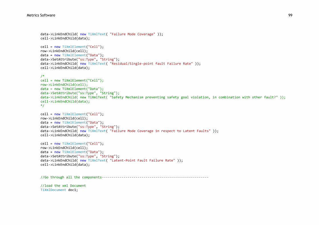
Metrics Software 99
data->LinkEndChild( new TiXmlText( "Failure Mode Coverage" )); cell->LinkEndChild(data); cell = new TiXmlElement("Cell"); row->LinkEndChild(cell); data = new TiXmlElement("Data"); data->SetAttribute("ss:Type", "String"); data->LinkEndChild( new TiXmlText( "Residual/Single-point fault Failure Rate" )); cell->LinkEndChild(data); /* cell = new TiXmlElement("Cell"); row->LinkEndChild(cell); data = new TiXmlElement("Data"); data->SetAttribute("ss:Type", "String"); data->LinkEndChild( new TiXmlText( "Safety Mechanism preventing safety goal violation, in combination with other fault?" )); cell->LinkEndChild(data); */ cell = new TiXmlElement("Cell"); row->LinkEndChild(cell); data = new TiXmlElement("Data"); data->SetAttribute("ss:Type", "String"); data->LinkEndChild( new TiXmlText( "Failure Mode Coverage in respect to Latent Faults" )); cell->LinkEndChild(data); cell = new TiXmlElement("Cell"); row->LinkEndChild(cell); data = new TiXmlElement("Data"); data->SetAttribute("ss:Type", "String"); data->LinkEndChild( new TiXmlText( "Latent-Point Fault Failure Rate" )); cell->LinkEndChild(data); //Go through all the components------------------------------------------------------ //load the xml Document TiXmlDocument doc1;
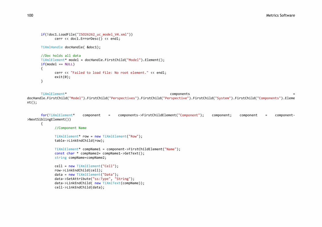
100 Metrics Software
if(!doc1.LoadFile("ISO26262_uc_model_V4.xml")) cerr << doc1.ErrorDesc() << endl; TiXmlHandle docHandle( &doc1); //Doc holds all data TiXmlElement* model = docHandle.FirstChild("Model").Element(); if(model == NULL) { cerr << "Failed to load file: No root element." << endl; exit(0); } TiXmlElement* components = docHandle.FirstChild("Model").FirstChild("Perspectives").FirstChild("Perspective").FirstChild("System").FirstChild("Components").Element(); for(TiXmlElement* component = components->FirstChildElement("Component"); component; component = component->NextSiblingElement()) { //Component Name TiXmlElement* row = new TiXmlElement("Row"); table->LinkEndChild(row); TiXmlElement* compName1 = component->FirstChildElement("Name"); const char * compName2= compName1->GetText(); string compName=compName2; cell = new TiXmlElement("Cell"); row->LinkEndChild(cell); data = new TiXmlElement("Data"); data->SetAttribute("ss:Type", "String"); data->LinkEndChild( new TiXmlText(compName)); cell->LinkEndChild(data);
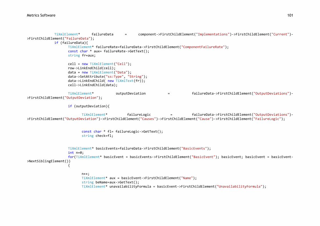
Metrics Software 101
TiXmlElement* failureData = component->FirstChildElement("Implementations")->FirstChildElement("Current")->FirstChildElement("FailureData"); if (failureData){ TiXmlElement* failureRate=failureData->FirstChildElement("ComponentFailureRate"); const char * aux= failureRate->GetText(); string fr=aux; cell = new TiXmlElement("Cell"); row->LinkEndChild(cell); data = new TiXmlElement("Data"); data->SetAttribute("ss:Type", "String"); data->LinkEndChild( new TiXmlText(fr)); cell->LinkEndChild(data); TiXmlElement* outputDeviation = failureData->FirstChildElement("OutputDeviations")->FirstChildElement("OutputDeviation"); if (outputDeviation){ TiXmlElement* failureLogic = failureData->FirstChildElement("OutputDeviations")->FirstChildElement("OutputDeviation")->FirstChildElement("Causes")->FirstChildElement("Cause")->FirstChildElement("FailureLogic"); const char * fl= failureLogic->GetText(); string check=fl; TiXmlElement* basicEvents=failureData->FirstChildElement("BasicEvents"); int n=0; for(TiXmlElement* basicEvent = basicEvents->FirstChildElement("BasicEvent"); basicEvent; basicEvent = basicEvent->NextSiblingElement()) { n++; TiXmlElement* aux = basicEvent->FirstChildElement("Name"); string beName=aux->GetText(); TiXmlElement* unavailabilityFormula = basicEvent->FirstChildElement("UnavailabilityFormula");

102 Metrics Software
if(unavailabilityFormula){ TiXmlElement* aux1 = unavailabilityFormula->FirstChildElement("Constant")->FirstChildElement("FailureRate"); const char * fr1=aux1->GetText(); string fr=aux1->GetText(); std::size_t found = beName.find("SM"); if(found==std::string::npos){ //If the Component has more than 1 relevant Failure Mode if(n>=2){ int t=n; TiXmlElement* row = new TiXmlElement("Row"); table->LinkEndChild(row); while (t>0){ cell = new TiXmlElement("Cell"); row->LinkEndChild(cell); t--; } //Failure Mode cell = new TiXmlElement("Cell"); row->LinkEndChild(cell); data = new TiXmlElement("Data"); data->SetAttribute("ss:Type", "String"); data->LinkEndChild( new TiXmlText(beName)); cell->LinkEndChild(data); //Failure Mode Failure Rate cell = new TiXmlElement("Cell"); row->LinkEndChild(cell); data = new TiXmlElement("Data"); data->SetAttribute("ss:Type", "String"); data->LinkEndChild( new TiXmlText(fr)); cell->LinkEndChild(data);
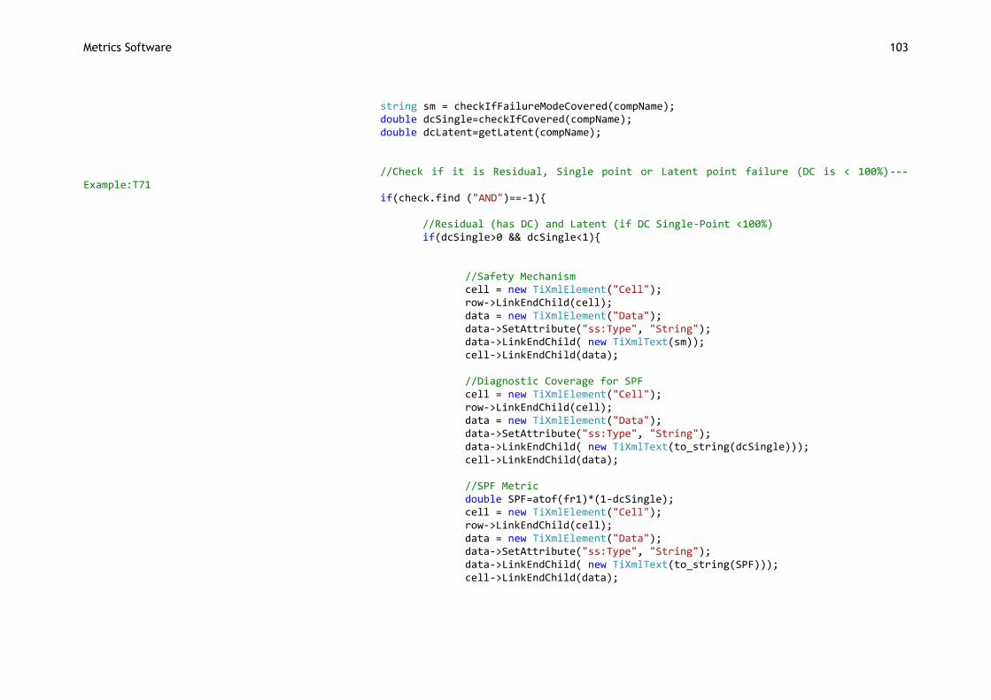
Metrics Software 103
string sm = checkIfFailureModeCovered(compName); double dcSingle=checkIfCovered(compName); double dcLatent=getLatent(compName); //Check if it is Residual, Single point or Latent point failure (DC is < 100%)---Example:T71 if(check.find ("AND")==-1){ //Residual (has DC) and Latent (if DC Single-Point <100%) if(dcSingle>0 && dcSingle<1){ //Safety Mechanism cell = new TiXmlElement("Cell"); row->LinkEndChild(cell); data = new TiXmlElement("Data"); data->SetAttribute("ss:Type", "String"); data->LinkEndChild( new TiXmlText(sm)); cell->LinkEndChild(data); //Diagnostic Coverage for SPF cell = new TiXmlElement("Cell"); row->LinkEndChild(cell); data = new TiXmlElement("Data"); data->SetAttribute("ss:Type", "String"); data->LinkEndChild( new TiXmlText(to_string(dcSingle))); cell->LinkEndChild(data); //SPF Metric double SPF=atof(fr1)*(1-dcSingle); cell = new TiXmlElement("Cell"); row->LinkEndChild(cell); data = new TiXmlElement("Data"); data->SetAttribute("ss:Type", "String"); data->LinkEndChild( new TiXmlText(to_string(SPF))); cell->LinkEndChild(data);
104 Metrics Software
//Perceived Faults cell = new TiXmlElement("Cell"); row->LinkEndChild(cell); data = new TiXmlElement("Data"); data->SetAttribute("ss:Type", "String"); data->LinkEndChild( new TiXmlText(to_string(dcLatent))); cell->LinkEndChild(data); //Latent-Point Failure Metric double LPF=((atof(fr1))-SPF)*(1-dcLatent); cell = new TiXmlElement("Cell"); row->LinkEndChild(cell); data = new TiXmlElement("Data"); data->SetAttribute("ss:Type", "String"); data->LinkEndChild( new TiXmlText(to_string(LPF))); cell->LinkEndChild(data); } //Single-Point Failure with no DC else if(dcSingle!=NULL && !(dcSingle>0 && dcSingle<=1)){ //No Safety Mechanism cell = new TiXmlElement("Cell"); row->LinkEndChild(cell); data = new TiXmlElement("Data"); data->SetAttribute("ss:Type", "String"); data->LinkEndChild( new TiXmlText("none")); cell->LinkEndChild(data); //Diagnostic Coverage is 0 cell = new TiXmlElement("Cell"); row->LinkEndChild(cell); data = new TiXmlElement("Data"); data->SetAttribute("ss:Type", "String"); data->LinkEndChild( new TiXmlText("0")); cell->LinkEndChild(data);
Metrics Software 105
//SPF Metric (just the Failure Rate of the Component) double SPF=atof(fr1); cell = new TiXmlElement("Cell"); row->LinkEndChild(cell); data = new TiXmlElement("Data"); data->SetAttribute("ss:Type", "String"); data->LinkEndChild( new TiXmlText(to_string(SPF))); cell->LinkEndChild(data); //No Latent Fault Diagnostic Coverage cell = new TiXmlElement("Cell"); row->LinkEndChild(cell); //No LPF Metric cell = new TiXmlElement("Cell"); row->LinkEndChild(cell); } //Component Fault that is not relevant for the Violation of the Safety goal else { cell = new TiXmlElement("Cell"); row->LinkEndChild(cell); cell = new TiXmlElement("Cell"); row->LinkEndChild(cell); cell = new TiXmlElement("Cell"); row->LinkEndChild(cell); cell = new TiXmlElement("Cell"); row->LinkEndChild(cell); cell = new TiXmlElement("Cell"); row->LinkEndChild(cell); } } //Only Latent with combination of failures else if(check.find ("AND")!=-1 && check.find ("external")!=-1){
106 Metrics Software
//No Safety Mechanism cell = new TiXmlElement("Cell"); row->LinkEndChild(cell); //No Single-Point Coverage cell = new TiXmlElement("Cell"); row->LinkEndChild(cell); //No Single-Point Failure Metric cell = new TiXmlElement("Cell"); row->LinkEndChild(cell); //Coverage for Latent Faults is 0 cell = new TiXmlElement("Cell"); row->LinkEndChild(cell); data = new TiXmlElement("Data"); data->SetAttribute("ss:Type", "String"); data->LinkEndChild( new TiXmlText("0")); cell->LinkEndChild(data); //Latent-Point Failure: Component AND external condition double LPF=atof(fr1); cell = new TiXmlElement("Cell"); row->LinkEndChild(cell); data = new TiXmlElement("Data"); data->SetAttribute("ss:Type", "String"); data->LinkEndChild( new TiXmlText(to_string(LPF))); cell->LinkEndChild(data); } } //If the Component has just 1 relevant Failure Mode else if (n<2){ //Failure Mode cell = new TiXmlElement("Cell");
Metrics Software 107
row->LinkEndChild(cell); data = new TiXmlElement("Data"); data->SetAttribute("ss:Type", "String"); data->LinkEndChild( new TiXmlText(beName)); cell->LinkEndChild(data); //Failure Mode Failure Rate cell = new TiXmlElement("Cell"); row->LinkEndChild(cell); data = new TiXmlElement("Data"); data->SetAttribute("ss:Type", "String"); data->LinkEndChild( new TiXmlText(fr)); cell->LinkEndChild(data); string sm = checkIfFailureModeCovered(compName); double dcSingle=checkIfCovered(compName); double dcLatent=getLatent(compName); //Check if it is Residual, Single point or Latent point failure (DC is < 100%)---Example:T71 if(check.find ("AND")==-1){ //Residual (has DC) and Latent (if DC Single-Point <100%) if(dcSingle>0 && dcSingle<1){ //Safety Mechanism cell = new TiXmlElement("Cell"); row->LinkEndChild(cell); data = new TiXmlElement("Data"); data->SetAttribute("ss:Type", "String"); data->LinkEndChild( new TiXmlText(sm)); cell->LinkEndChild(data); //Diagnostic Coverage for SPF cell = new TiXmlElement("Cell"); row->LinkEndChild(cell);
108 Metrics Software
data = new TiXmlElement("Data"); data->SetAttribute("ss:Type", "String"); data->LinkEndChild( new TiXmlText(to_string(dcSingle))); cell->LinkEndChild(data); //SPF Metric double SPF=atof(fr1)*(1-dcSingle); cell = new TiXmlElement("Cell"); row->LinkEndChild(cell); data = new TiXmlElement("Data"); data->SetAttribute("ss:Type", "String"); data->LinkEndChild( new TiXmlText(to_string(SPF))); cell->LinkEndChild(data); //Perceived Faults cell = new TiXmlElement("Cell"); row->LinkEndChild(cell); data = new TiXmlElement("Data"); data->SetAttribute("ss:Type", "String"); data->LinkEndChild( new TiXmlText(to_string(dcLatent))); cell->LinkEndChild(data); //Latent-Point Failure Metric double LPF=((atof(fr1))-SPF)*(1-dcLatent); cell = new TiXmlElement("Cell"); row->LinkEndChild(cell); data = new TiXmlElement("Data"); data->SetAttribute("ss:Type", "String"); data->LinkEndChild( new TiXmlText(to_string(LPF))); cell->LinkEndChild(data); } //Single-Point Failure with no DC else if(dcSingle!=NULL && !(dcSingle>0 && dcSingle<=1)){ //No Safety Mechanism cell = new TiXmlElement("Cell");
Metrics Software 109
row->LinkEndChild(cell); data = new TiXmlElement("Data"); data->SetAttribute("ss:Type", "String"); data->LinkEndChild( new TiXmlText("none")); cell->LinkEndChild(data); //Diagnostic Coverage is 0 cell = new TiXmlElement("Cell"); row->LinkEndChild(cell); data = new TiXmlElement("Data"); data->SetAttribute("ss:Type", "String"); data->LinkEndChild( new TiXmlText("0")); cell->LinkEndChild(data); //SPF Metric (just the Failure Rate of the Component) double SPF=atof(fr1); cell = new TiXmlElement("Cell"); row->LinkEndChild(cell); data = new TiXmlElement("Data"); data->SetAttribute("ss:Type", "String"); data->LinkEndChild( new TiXmlText(to_string(SPF))); cell->LinkEndChild(data); //No Latent Fault Diagnostic Coverage cell = new TiXmlElement("Cell"); row->LinkEndChild(cell); //No LPF Metric cell = new TiXmlElement("Cell"); row->LinkEndChild(cell); } //Component Fault that is not relevant for the Violation of the Safety goal else { cell = new TiXmlElement("Cell"); row->LinkEndChild(cell); cell = new TiXmlElement("Cell");
110 Metrics Software
row->LinkEndChild(cell); cell = new TiXmlElement("Cell"); row->LinkEndChild(cell); cell = new TiXmlElement("Cell"); row->LinkEndChild(cell); cell = new TiXmlElement("Cell"); row->LinkEndChild(cell); } } //Only Latent with combination of failures else if(check.find ("AND")!=-1 && check.find ("external")!=-1){ //No Safety Mechanism cell = new TiXmlElement("Cell"); row->LinkEndChild(cell); //No Single-Point Coverage cell = new TiXmlElement("Cell"); row->LinkEndChild(cell); //No Single-Point Failure Metric cell = new TiXmlElement("Cell"); row->LinkEndChild(cell); //Coverage for Latent Faults is 0 cell = new TiXmlElement("Cell"); row->LinkEndChild(cell); data = new TiXmlElement("Data"); data->SetAttribute("ss:Type", "String"); data->LinkEndChild( new TiXmlText("0")); cell->LinkEndChild(data); //Latent-Point Failure: Component AND external condition double LPF=atof(fr1); cell = new TiXmlElement("Cell"); row->LinkEndChild(cell);
Metrics Software 111
data = new TiXmlElement("Data"); data->SetAttribute("ss:Type", "String"); data->LinkEndChild( new TiXmlText(to_string(LPF))); cell->LinkEndChild(data); } } } } } n=0; } } } //Total Residual+Single Failure Rates and Latent Failure Rate getMetrics(); string sp=to_string(SPMetric); string lp=to_string(LPMetric); TiXmlElement* row1 = new TiXmlElement("Row");
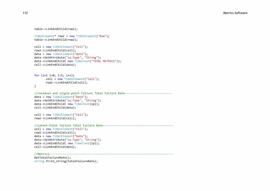
112 Metrics Software
table->LinkEndChild(row1); TiXmlElement* row2 = new TiXmlElement("Row"); table->LinkEndChild(row2); cell = new TiXmlElement("Cell"); row2->LinkEndChild(cell); data = new TiXmlElement("Data"); data->SetAttribute("ss:Type", "String"); data->LinkEndChild( new TiXmlText("TOTAL METRICS")); cell->LinkEndChild(data); for (int i=0; i<5; i++){ cell = new TiXmlElement("Cell"); row2->LinkEndChild(cell); } //residual and single-point Failure Total Failure Rate---------------------------- data = new TiXmlElement("Data"); data->SetAttribute("ss:Type", "String"); data->LinkEndChild( new TiXmlText(sp)); cell->LinkEndChild(data); cell = new TiXmlElement("Cell"); row2->LinkEndChild(cell); //Latent-Point Failure Total Failure Rate------------------------------------------ cell = new TiXmlElement("Cell"); row2->LinkEndChild(cell); data = new TiXmlElement("Data"); data->SetAttribute("ss:Type", "String"); data->LinkEndChild( new TiXmlText(lp)); cell->LinkEndChild(data); //Metrics-------------------------------------------------------------------------- GetTotalFailureRate(); string fr=to_string(totalFailureRate);
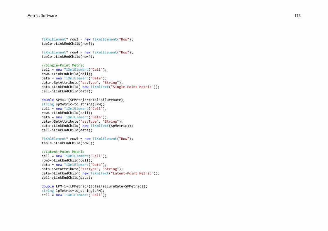
Metrics Software 113
TiXmlElement* row3 = new TiXmlElement("Row"); table->LinkEndChild(row3); TiXmlElement* row4 = new TiXmlElement("Row"); table->LinkEndChild(row4); //Single-Point Metric cell = new TiXmlElement("Cell"); row4->LinkEndChild(cell); data = new TiXmlElement("Data"); data->SetAttribute("ss:Type", "String"); data->LinkEndChild( new TiXmlText("Single-Point Metric")); cell->LinkEndChild(data); double SPM=1-(SPMetric/totalFailureRate); string spMetric=to_string(SPM); cell = new TiXmlElement("Cell"); row4->LinkEndChild(cell); data = new TiXmlElement("Data"); data->SetAttribute("ss:Type", "String"); data->LinkEndChild( new TiXmlText(spMetric)); cell->LinkEndChild(data); TiXmlElement* row5 = new TiXmlElement("Row"); table->LinkEndChild(row5); //Latent-Point Metric cell = new TiXmlElement("Cell"); row5->LinkEndChild(cell); data = new TiXmlElement("Data"); data->SetAttribute("ss:Type", "String"); data->LinkEndChild( new TiXmlText("Latent-Point Metric")); cell->LinkEndChild(data); double LPM=1-(LPMetric/(totalFailureRate-SPMetric)); string lpMetric=to_string(LPM); cell = new TiXmlElement("Cell");
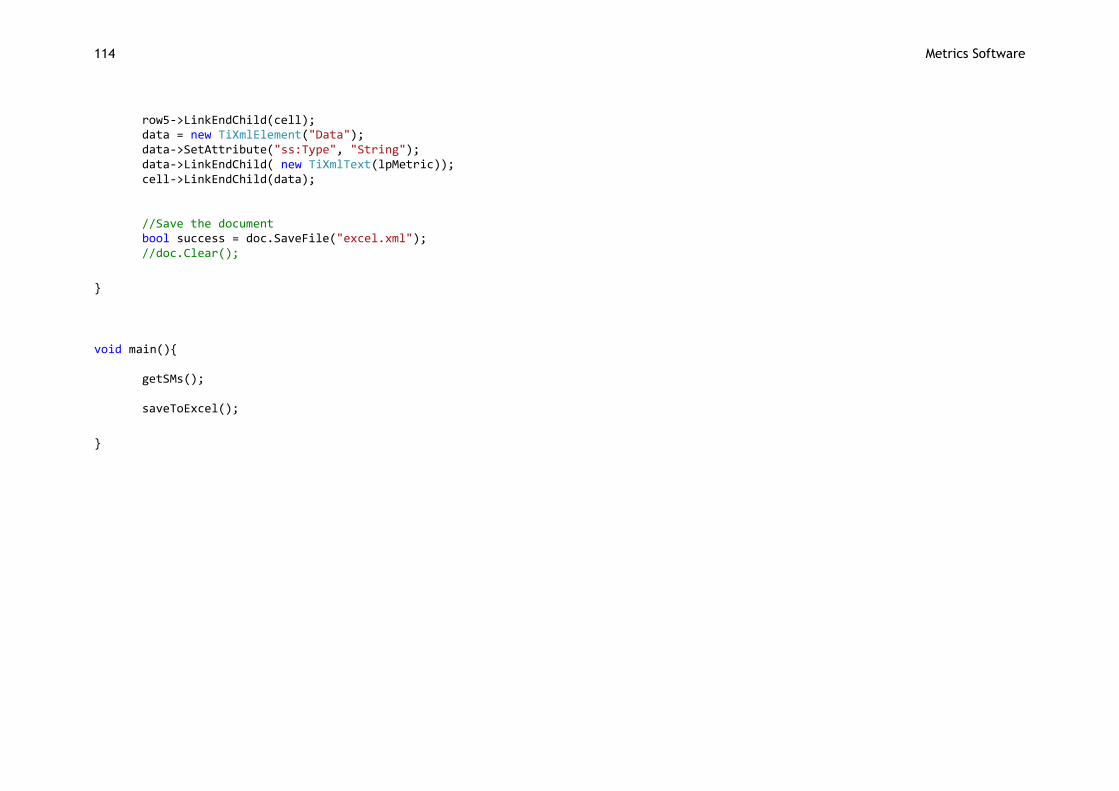
114 Metrics Software
row5->LinkEndChild(cell); data = new TiXmlElement("Data"); data->SetAttribute("ss:Type", "String"); data->LinkEndChild( new TiXmlText(lpMetric)); cell->LinkEndChild(data); //Save the document bool success = doc.SaveFile("excel.xml"); //doc.Clear();
}
void main(){ getSMs(); saveToExcel();
}