Automatic Verification of DynamicData-Dependent Programs

Parosh Aziz Abdulla1, Muhsin Atto1, Jonathan Cederberg1, Ran Ji1.

1 Uppsala University, Sweden.

Abstract. We present a new approach for automatic verification ofdata-dependent programs manipulating dynamic heaps. A heap is en-coded by a graph where the nodes represent the cells, and the edgesreflect the pointer structure between the cells of the heap. Each cellcontains a set of variables which range over the natural numbers. Ourmethod relies on standard backward reachability analysis, where themain idea is to use a simple set of predicates, called signatures, in orderto represent bad sets of heaps. Examples of bad heaps are those whichcontain either garbage, lists which are not well-formed, or lists which arenot sorted. We present the results for the case of programs with a singlenext-selector, and where variables may be compared for equality or in-equality. This allows us to verify for instance that a program, like bubblesort or insertion sort, returns a list which is well-formed and sorted, orthat the merging of two sorted lists is a new sorted list. We will reporton the result of running a prototype based on the method on a numberof programs.

1 Introduction

We consider automatic verification of data-dependent programs that manipulatedynamic linked lists. The contents of the linked lists, here refered to as a heap, isrepresented by a graph. The nodes of the graph represent the cells of the heap,while the edges reflect the pointer structure between the cells (see Figure 1 for atypical example). The program has a dynamic behaviour in the sense that cellsmay be created and deleted; and that pointers may be re-directed during theexecution of the program. The program is also data-dependent since the cellscontain variables, ranging over the natural numbers, that can be compared for(in)equality and whose values may be updated by the program. The values ofthe local variables are provided as attributes to the corresponding cells. Finally,we have a set of (pointer) variables which point to different cells inside the heap.

In this paper, we consider the case of programs with a single next-selector,i.e., where each cell has at most one successor. For this class of programs, we pro-vide a method for automatic verification of safety properties. Such properties canbe either structural properties such as absence of garbage, sharing, and danglingpointers; or data properties such as sortedness. We provide a simple symbolic rep-resentation, which we call signatures, for characterizing (infinite) sets of heaps.Signatures can also be represented by graphs. The difference, compared to thecase of heaps, is that some parts may be “missing” from the graph of a signa-ture. For instance, the absence of a pointer means that the pointer may point

to an arbitrary cell inside a heap satisfying the signature. In this manner, a sig-nature can be interpreted as a forbidden pattern which should not occur insidethe heap. The forbidden pattern is essentially a set of minimal conditions whichshould be satisfied by any heap in order for the heap to satisfy the signature.A heap satisfying the signature is considered to be bad in the sense that it con-tains a bad pattern which in turn implies that it violates one of the propertiesmentioned above. Examples of bad patterns in heaps are garbage, lists whichare not well-formed, or lists which are not sorted. This means that checking asafety property amounts to checking the reachability of a finite set of signatures.We perform standard backward reachability analysis, using signatures as a sym-bolic representation, and starting from the set of bad signatures. We show howto perform the two basic operations needed for backward reachability analysis,namely checking entailment and computing predecessors on signatures.

For checking entailment, we define a pre-order v on signatures, where weview a signature as three separate graphs with identical sets of nodes. The edgerelation in one of the three graphs reflects the structure of the heap graph, whilethe other two reflect the ordering on the values of the variables (equality resp.inequality). Given two signatures g1 and g2, we have g1 v g2 if g1 can be obtainedfrom g2 by a sequence of transformations consisting of either deleting an edge (inone of the three graphs), a variable, an isolated node, or contracting segments(i.e., sequence of nodes) without sharing in the structure graph. In fact, thisordering also induces an ordering on heaps where h1 v h2 if, for all signaturesg, h2 satisfies g whenever h1 satisfies g.

When performing backward reachability analysis, it is essential that the un-derlying symbolic representation, signatures in our case, is closed under theoperation of computing predecessors. More precisely, for a signature g, let usdefine Pre(g) to be the set of predecessors of g, i.e., the set of signatures whichcharacterize those heaps from which we can perform one step of the programand as a result obtain a heap satisfying g. Unfortunately, the set Pre(g) doesnot exist in general under the operational semantics of the class of programs weconsider in this paper. Therefore, we consider an over-approximation of the tran-sition relation where a heap h is allowed first to move to smaller heap (w.r.t. theordering v) before performing the transition. For the approximated transitionrelation, we show that the set Pre(g) exists, and that it is finite and computable.

One advantage of using signatures is that it is quite straightforward to specifysets of bad heaps. For instance, forbidden patterns for the properties of list well-formedness and absence of garbage can each be described by 4-6 signatures,with 2-3 nodes in each signature. Also, the forbidden pattern for the propertythat a list is sorted consists of only one signature with two nodes. Furthermore,signatures offer a very compact symbolic representation of sets of bad heaps. Infact, when verifying our programs, the number of nodes in the signatures whicharise in the analysis does not exceed ten. In addition, the rules for computingpredecessors are local in the sense that they change only a small part of thegraph (typically one or two nodes and edges). This makes it possible to checkentailment and compute predecessors quite efficiently.

The whole verification process is fully automatic since both the approxima-tion and the reachability analysis are carried out without user intervention. No-tice that if we verify a safety property in the approximate transition system thenthis also implies its correctness in the original system. We have implemented aprototype based on our method, and carried out automatic verification of severalprograms such as insertion in a sorted lists, bubble sort, insertion sort, mergingof sorted lists, list partitioning, reversing sorted lists, etc. Although the proce-dure is not guaranteed to terminate in general, our prototype terminates on allthese examples.Related Work Several works consider the verification of singly linked listswith data. The paper [12] presents a method for automatic verification of sort-ing programs that manipulate linked lists. The method is defined within theframework of TVLA which provides an abstract description of the heap struc-tures in 3-valued logic [17]. The user may be required to provide instrumentationpredicates in order to make the abstraction sufficiently precise. The analysis isperformed in a forward manner. In contrast, the search procedure we describe inthis paper is backward, and therefore also property-driven. Thus, the signaturesobtained in the traversal do not need to express the state of the entire heap,but only those parts that contribute to the eventual failure. This makes the twomethods conceptually and technically different. Furthermore, the difference insearch strategy implies that forward and backward search procedures often offervarying degrees of efficiency in different contexts, which makes them complemen-tary to each other in many cases. This has been observed also for other modelssuch as parameterized systems, timed Petri nets, and lossy channel systems (seee.g. [4, 9, 1]).

Another approach to verification of linked lists with data is proposed in [6,7] based on abstract regular model checking (ARMC) [8]. In ARMC, finite-stateautomata are used as a symbolic representation of sets of heaps. This means thatthe ARMC-based approach needs the manipulation of quite complex encodingsof the heap graphs into words or trees. In contrast, our symbolic representationuses signatures which provide a simpler and more natural representation of heapsas graphs. Furthermore, ARMC uses a sophisticated machinery for manipulat-ing the heap encodings based on representing program statements as (word/tree)transducers. However, as mentioned above, our operations for computing prede-cessors are all local in the sense that they only update limited parts of the graphthus making it possible to have much more efficient implementations.

The paper [5] uses counter automata as abstract models of heaps whichcontain data from an ordered domain. The counters are used to keep track oflengths of list segments without sharing. The analysis reduces to manipulationof counter automata, and thus requires techniques and tools for these automata.

Recently, there has been an extensive work to use separation logic [16] forperforming shape analysis of programs that manipulate pointer data structures(see e.g. [10, 19]). The paper [14] describes how to use separation logic in orderto provide a semi-automatic procedure for verifying data-dependent programswhich manipulate heaps. In contrast, the approach we present here uses a built-

in abstraction principle which is different from the ones used above and whichmakes the analysis fully automatic.

The tool PALE (Pointer Assertion Logic Engine) [13] checks automaticallyproperties of programs manipulating pointers. The user is required to supplyassertions expressed in the weak monadic second-order logic of graph types. Thismeans that the verification procedure as a whole is only partially automatic. Thetool MONA [11], which uses translations to finite-state automata, is employedto verify the provided assertions.

In our previous work [3], we used backward reachability analysis for verifyingheap manipulating programs. However, the programs are restricted to be data-independent. The extension to the case of data-dependent programs is not trivialand requires an intricate treatment of the ordering on signatures. In particular,the interaction between the structural and the data orderings is central to ourmethod. This is used for instance to specify basic properties like sortedness(whose forbidden pattern contains edges from both orderings). Hence, none ofthe programs we consider in this paper can be analyzed in the framework of [3].Outline In the next section, we describe our model of heaps, and introduce theprogramming language together with the induced transition system. In Section 3,we introduce the notion of signatures and the associated ordering. Section 4describes how to specify sets of bad heaps using signatures. In Section 5 we givean overview of the backward reachability scheme, and show how to computethe predecessor relation on signatures. The experimental results are presentedin Section 6. Finally, in Section 7 we give some conclusions and directions forfuture research. Definitions of some of the operations, and descriptions of thecase studies are given in the appendix and in [2].

2 Heaps

In this section, we give some preliminaries on programs which manipulate heaps.Let N be the set of natural numbers. For sets A and B, we write f : A→ B

to denote that f is a (possibly partial) function from A to B. We write f(a) = ⊥to denote that f(a) is undefined. We use f [a← b] to denote the function f ′

such that f ′(a) = b and f ′(x) = f(x) if x 6= a. In particular, we use f [a← ⊥]to denote the function f ′ which agrees on f on all arguments, except that f ′(a)is undefined.Heaps We consider programs which operate on dynamic data structures, herecalled heaps. A heap consists of a set of memory cells (cells for short), whereeach cell has one next-pointer. Examples of such heaps are singly liked lists andcircular lists, possibly sharing their parts (see Figure 1). A cell in the heap maycontain a datum which is a natural number. A program operating on a heapmay use a finite set of variables representing pointers whose values are cellsinside the heap. A pointer may have the special value null which represents acell without successors. Furthermore, a pointer may be dangling which meansthat it does not point to any cell in the heap. Sometimes, we write the “x-

cell” to refer to the the cell pointed to by the variable x. We also write “thevalue of the x-cell” to refer to the value stored inside the cell pointed to by x.

5 6x

1

6

y

3v

4z

# ∗w

Fig. 1. A typical graph representing the heap.

A heap cannaturally beencoded bya graph, asthe one ofFigure 1. Avertex in thegraph rep-resents a cellin the heap,while the edges reflect the successor (pointer) relation on the cells. A variableis attached to a vertex in the graph if the variable points to the correspondingcell in the heap. Cell values are written inside the nodes (absence of a numbermeans that the value is undefined).

Assume a finite setX of variables. Formally, a heap is a tuple (M,Succ, λ,Val)where

– M is a finite set of (memory) cells. We assume two special cells # and ∗ whichrepresent the constant null and the dangling pointer value respectively. Wedefine M• := M ∪ {#, ∗}.

– Succ : M → M•. If Succ(m1) = m2 then the (only) pointer of the cell m1

points to the cell m2. The function Succ is total which means that each cellin M has a successor (possibly # or ∗). Notice that the special cells # and∗ have no successors.

– λ : X → M• defines the cells pointed to by the variables. The function λ istotal, i.e., each variable points to one cell (possibly # or ∗).

– Val : M → N is a partial function which gives the values of the cells.

In Figure 1, we have 17 cells of which 15 are in M , The set X is given by{x, y, z, v, w}. The successor of the z-cell is null. Variable w is attached to thecell ∗, which means that w is dangling (w does not point to any cell in the heap).Furthermore, the value of the x-cell is 6, the value of the y-cell is not defined,the value of the successor of the y-cell is 3, etc.Remark In fact, we can allow cells to contain multiple values. However, tosimplify the presentation, we keep the assumption that a cell contains only onenumber. This will be sufficient for our purposes; and furthermore, all the defini-tions and methods we present in the paper can be extended in a straightforwardmanner to the general case. Furthermore, we can use ordered domains other thanthe natural numbers such as the integers, rationals, or reals.Programming Language We define a simple programming language. To thisend, we assume, together with the earlier mentioned set X of variables, theconstant null where null 6∈ X. We define X# := X ∪ {null}. A programP is a pair (Q,T ) where Q is a finite set of control states and T is a finiteset of transitions. The control states represent the locations of the program. Atransition is a triple (q1, op, q2) where q1, q2 ∈ Q are control states and op is an

operation. In the transition, the program changes location from q1 to q2, while itchecks and manipulates the heap according to the operation op. The operationop is of one of the following forms

– x = y or x 6= y where x, y ∈ X#. The program checks whether the x- andy-cells are identical or different.

– x := y or x.next := y where x ∈ X and y ∈ X#. In the first operation,the program makes x point to the y-cell, while in the second operation itupdates the successor of the x-cell, and makes it equal to the y-cell.

– x := y.next where x, y ∈ X. The variable x will now point to the successorof the y-cell.

– new(x), delete(x), or read(x ), where x ∈ X. The first operation creates anew cell and makes x point to it; the second operation removes the x-cellfrom the heap; while the third operation reads a new value and assigns it tothe x-cell.

– x.num = y.num, x.num < y.num, x.num := y.num, x.num :> y.num,or x.num :< y.num, where x, y ∈ X. The first two operations compare thevalues of (number stored inside) the x- and y-cells. The third operation copiesthe value of the y-cell to the x-cell. The fourth (fifth) operation assigns non-deterministically a value to the x-cell which is larger (smaller) than that ofthe y-cell.

Figure 2 illustrates the effect of a sequence of operations of the forms describedabove on a number of heaps. Examples of some programs can be found in theappendix and in [2].

6

x1

6

y

z

3

h0

6

x1

6

y

9

z

3

h1

6

1

6

y

9

z

3 x

h2

6

1

6

y

9

z

∗x

h3

6

1

6

y

9

z

∗x

h4

6

1

6

y

9

z

∗x

h5

Fig. 2. Starting from the heap h0, the heaps h1, h2, h3, h4, and h5 are generatedby performing the following sequence of operations: z.num :> x.num, x := y.next ,delete(x), new(x), and z.next := y. To simplify the figures, we omit the special nodes# and ∗ unless one of the variables x, y, z is attached to them. For this reason the cell# is missing in all the heaps, and ∗ is present only in h3, h4, h5.

Transition System We define the operational semantics of a program P =(Q,T ) by giving the transition system induced by P . In other words, we definethe set of configurations and a transition relation on configurations. A configu-ration is a pair (q, h) where q ∈ Q represents the location of the program, and his a heap.

We define a transition relation (on configurations) that reflects the mannerin which the instructions of the program change a given configuration. First,we define some operations on heaps. Fix a heap h = (M,Succ, λ,Val). Form1,m2 ∈ M , we use (h.Succ) [m1 ← m2] to denote the heap h′ we obtain byupdating the successor relation such that the cell m2 now becomes the successorof m1 (without changing anything else in h). Formally, h′ =

(M,Succ′,Val , λ

)where Succ′ = Succ [m1 ← m2]. Analogously, (h.λ) [x← m] is the heap we ob-tain by making x point to the cell m; and (h.Val) [m← i] is the heap weobtain by assigning the value i to the cell m. For instance, in Figure 2, lethi be of the form (Mi,Succi,Val i, λi) for i ∈ {0, 1, 2, 3, 4, 5}. Then, we haveh1 = (h0.Val) [λ0(z)← 9] since we make the value of the z-cell equal to 9. Also,h2 = (h1.λ1) [x← Succ1(λ1(y))] since we make x point to the successor of they-cell. Furthermore, h5 = (h4.Succ4) [λ4(z)← λ4(y)] since we make the y-cellthe successor of the z-cell.

Consider a cell m ∈M . We define hm to be the heap h′ we get by deletingthe cell m from h. More precisely, we define h′ :=

(M ′,Succ′, λ′,Val ′

)where

– M ′ = M − {m}.– Succ′(m′) = Succ(m′) if Succ(m′) 6= m, and Succ′(m′) = ∗ otherwise. In

other words, the successor of cells pointing to m will become dangling in h′.– λ′(x) = ∗ if λ(x) = m, and λ′(x) = λ(x) otherwise. In other words, variables

pointing to the same cell as x in h will become dangling in h′.– Val ′(m′) = Val(m′) if m′ ∈M ′. That is, the function Val ′ is the restriction

of Val to M ′: it assigns the same values as Val to all the cells which remainin M ′ (since m 6∈M ′, it not meaningful to speak about Val (m)).

In Figure 2, we have h3 = h2 λ2(x).Let t = (q1, op, q2) be a transition and let c = (q, h) and c′ = (q′, h′) be

configurations. We write c t−→ c′ to denote that q = q1, q′ = q2, and hop−→ h′,

where hop−→ h′ holds if we obtain h′ by performing the operation op on h. For

brevity, we give the definition of the relationop−→ for three types of operations.

The rest of the cases can be found in the appendix.

– op is of the form x := y.next , λ(y) ∈ M , Succ(λ(y)) 6= ∗, and h′ =(h.λ) [x← Succ(λ(y))].

– op is of the from new(x), M ′ = M ∪ {m} for some m 6∈M , λ′ = λ [x← m],Succ′ = Succ [m← ∗], Val ′(m′) = Val(m′) if m′ 6= m, and Val ′(m) = ⊥.This operation creates a new cell and makes x point to it. The value of thenew cell is not defined, while the successor is the special cell ∗. As an exampleof this operation, see the transition from h3 to h4 in Figure 2.

– op is of the form x.num :> y.num, λ(x) ∈ M , λ(y) ∈ M , Val(λ(y)) 6= ⊥,and h′ = (h.Val) [λ(x)← i], where i > Val(λ(y)).

We write c −→ c′ to denote that c t−→ c′ for some t ∈ T ; and use ∗−→ to denotethe reflexive transitive closure of −→. The relations −→ and ∗−→ are extendedto sets of configurations in the obvious manner.Remark One could also allow deterministic assignment operations of the formx.num := y.num + k or x.num := y.num − k for some constant k. However,according the approximate transition relation which we define in Section 5, theseoperations will have identical interpretations as the non-deterministic operationsgiven above.

3 Signatures

In this section, we introduce the notion of signatures. We will define an orderingon signatures from which we derive an ordering on heaps. We will then showhow to use signatures as a symbolic representation of infinite sets of heaps.Signatures Roughly speaking, a signature is a graph which is “less concrete”than a heap in the following sense:

– We do not store the actual values of the cells in a signature. Instead, wedefine an ordering on the cells which reflects their values.

– The functions Succ and λ in a signature are partial (in contrast to a heapin which these functions are total).

Formally, a signature g is a tuple of the form (M,Succ, λ,Ord), where M , Succ,λ are defined in the same way as in heaps (Section 2), except that Succ and λare now partial. Furthermore, Ord is a partial function from M ×M to the set{≺,≡}. Intuitively, if Succ(m) = ⊥ for some cell m ∈ M , then this means thatg puts no constraints on the successor of m, i.e., the successor of m can be anyarbitrary cell. Analogously, if λ(x) = ⊥, then x may point to any of the cells. Therelation Ord constrains the ordering on the cell values. If Ord(m1,m2) =≺ thenthe value of m1 is strictly smaller than that of m2; and if Ord(m1,m2) =≡ thentheir values are equal. This means that we abstract away the actual values of thecells, and only keep track of their ordering (and whether they are equal). For acell m, we say that the value of m is free if Ord(m,m′) = ⊥ and Ord(m′,m) = ⊥for all other cells m′. Abusing notation, we write m1 ≺ m2 (resp. m1 ≡ m2) ifOrd(m1,m2) =≺ (resp. Ord(m1,m2) =≡).

We represent signatures graphically in a manner similar to that of heaps.Figure 3 shows graphical representations of six signatures g0, . . . , g5 over theset of variables {x, y, z}. If a vertex in the graph has no successor, then thesuccessor of the corresponding cell is not defined in g (e.g., the y-cell in g4).Also, if a variable is missing in the graph, then this means that the cell to whichthe variable points is left unspecified (e.g., variable z in g3). The ordering Ordon cells is illustrated by dashed arrows. A dashed single-headed arrow from acell m1 to a cell m2 indicates that m1 ≺ m2. A dashed double-headed arrowbetween m1 and m2 indicates that m1 ≡ m2. To simplify the figures, we omitself-loops indicating value reflexivity (i.e., m ≡ m). We can view a signature asthree graphs with a common set of vertices, and with three edge relations; where

the first edge relation gives the graph structure, and the other two define theordering on cell values (inequality resp. equality)

x

y

z

g0

x

y

z

g1

x

y

z

g2

x

yg3

x

yg4

x

yg5

Fig. 3. Examples of signatures.

In fact, each heap h =(M,Succ, λ,Val) induces a uniquesignature which we denote bysig (h). More precisely, sig (h) :=(M,Succ, λ,Ord) where, for allcells m1,m2 ∈ M , we havem1 ≺ m2 iff Val(m1) <Val(m2) and m1 ≡ m2 iffVal(m1) = Val(m2). In otherwords, in the signature of h,we remove the concrete valuesin the cells and replace themby the ordering relation on thecell values. For example, in Fig-ure 2 and Figure 3, we haveg0 = sig (h0).Ordering We define an order-ing v on signatures. The in-tuition is that each signaturecan be interpreted as a predi-cate which characterizes an in-finite set of heaps. The ordering

is then the inverse of implication: smaller signatures impose less restrictions andhence characterize larger sets of heaps. We derive a small signature from a largerone, by deleting cells, edges, variables in the graph of the signature, and by weak-ening the ordering requirements on the cells (the latter corresponds to deletingedges encoding the two relations on data values). To define the ordering, wegive first definitions and describe some operations on signatures. Fix a signatureg = (M,Succ, λ,Ord).

A cell m ∈M is said to be semi-isolated if there is no x ∈ X with λ(x) = m,the value of m is free, Succ−1(m) = ∅, and either Succ(m) = ⊥ or Succ(m) = ∗.In other words, m is not pointed to by any variables, its value is not relatedto that of any other cell, it has no predecessors, and it has no successors (ex-cept possibly ∗). We say that m is isolated if it is semi-isolated and in additionSucc(m) = ⊥. A cell m ∈ M is said to be simple if there is no x ∈ X withλ(x) = m, the value of m is free, |Succ−1(m)| = 1, and Succ(m) 6= ⊥. In otherwords, m has exactly one predecessor, one successor and no label. In Figure 3,the topmost cell of g3 is isolated, and the successor of the x-cell in g4 is simple.In Figure 1, the cell to the left of the w-cell is semi-isolated in the signature ofthe heap.

The operations (g.Succ) [m1 ← m2] and (g.λ) [x← m] are defined in identicalfashion to the case of heaps. Furthermore, for cells m1,m2 and 2 ∈ {≺,≡,⊥},we define (g.Ord) [(m1,m2)← 2] to be the signature g′ we obtain from g by

making the ordering relation between m1 and m2 equal to 2. For a variable x,we define g x to be the signature g′ we get from g by deleting the variable xfrom the graph, i.e., g′ = (g.λ) [x← ⊥]. For a cell m, we define the signatureg′ = gm =

(M ′,Succ′, λ′,Ord ′

)in a manner similar to the case of heaps. The

only difference is that Ord ′ (rather than Val ′) is the restriction of Ord to pairsof cells both of which are different from m.

Now, we are ready to define the ordering. For signatures g = (M,Succ, λ,Ord)and g′ =

(M ′,Succ′, λ′,Ord ′

), we write that g � g′ to denote that one of the

following properties is satisfied:

– Variable Deletion: g = g′ x for some variable x,– Cell Deletion: g = g′ m for some isolated cell m ∈M ′,– Edge Deletion: g = (g′.Succ) [m← ⊥] for some m ∈M ′,– Contraction: there are cells m1,m2,m3 ∈ M ′ and a signature g1 such thatm2 is simple, Succ′(m1) = m2, Succ′(m2) = m3, g1 = (g′.Succ) [m1 ← m3]and g = g1 m2, or

– Order Deletion: g = (g′.Ord) [(m1,m2)← ⊥] for some cells m1,m2 ∈M ′.

We write g v g′ to denote that there are g0�g1�g2�· · ·�gn with n ≥ 0, g0 = g,and gn = g′. That is, we can obtain g from g′ by performing a finite sequenceof variable deletion, cell deletion, edge deletion, order deletion, and contractionoperations. In Figure 3 we obtain: g1 from g0 through three order deletions; g2from g1 through one order deletion; g3 from g2 through one variable deletion andtwo edge deletions; g4 from g3 through one node deletion and one edge deletion;and g5 from g4 through one contraction. It means that g5 �g4 �g3 �g2 �g1 �g0and hence g5 v g0

We define an ordering v on heaps such that h v h′ iff sig (h) v sig (h′). For aheap h and a signature g, we say that h satisfies g, denoted h |= g, if g v sig (h).In this manner, each signature characterizes an infinite set of heaps, namely theset [[g]] := {h|h |= g}. Notice that [[g]] is upward closed w.r.t. the ordering v onheaps. We also observe that, for signatures g and g′, we have that g v g′ iff[[g′]] ⊆ [[g]]. For a (finite) set G of signatures we define [[G]] :=

⋃g∈G [[g]].

Considering the heaps of Figure 2 and the signatures of Figure 3, we haveh1 |= g0, h2 6|= g0, h0 v h1, h0 6v h2, g1 v g0, etc.Remark Our definition implies that signatures cannot specify “exact distances”between cells. For instance, we cannot specify the set of heaps in which the x-celland the y-cell are exactly of distance one from each other. In fact, if such a heapis in the set then, since we allow contraction, heaps where the distance is largerthan one will also be in the set. On the other hand, we can characterize sets ofheaps where two cells are at distance at least k from each other for some k ≥ 1.

It is also worth mentioning that the classical graph minor relation is tooweak for our class of programs. The reason is that the contraction operation isinsensitive to the directions of the edges; and furthermore the ordering allowsmerging vertices which carry different labels (different variables). This meansthat for almost all the programs considered in this paper, we would get spuriousexamples falsifying the safety property.

4 Bad Configurations

In this section, we show how to use signatures in order to specify sets of bad heapsfor programs which produce ordered linear lists. A signature is interpreted as aforbidden pattern which should not occur inside the heap. Typically, we wouldlike such a program to produce a heap which is a linear list. Furthermore, theheap should not contain any garbage, and the output list should be ordered. Foreach of these three properties, we describe the corresponding forbidden patternsas a set of signatures which characterize exactly those heaps which violate theproperty. Later, we will collect all these signatures into a single set which exactlycharacterizes the set of bad configurations.

First, we give some definitions. Fix a heap h = (M,Succ, λ,Val). A loop inh is a set {m0, . . . ,mn} of cells such that Succ(mi) = mi+1 for all i : 0 ≤ i < n,and Succ(mn) = m0. For cells m,m′ ∈ M , we say that m′ is visible from m ifthere are cells m0,m1, . . . ,mn for some n ≥ 0 such that m0 = m, mn = m′,and mi+1 = Succ(mi) for all i : 0 ≤ i < n. In other words, there is a (possiblyempty) path in the graph leading from m to m′. We say that m′ is strictly visiblefrom m if n > 0 (i.e. the path is not empty). A set M ′ ⊆M is said to be visiblefrom m if some m′ ∈M ′ is visible from m. x

∗b1: b2: ∗x

xb3: b4: x

Well-Formedness We say that h is well-formed w.r.ta variable x if # is visible form the x-cell. Equivalently,neither the cell ∗ nor any loop is visible from the x-cell. Intuitively, if a heap satisfies this condition, thenthe part of the heap visible from the x-cell forms a linear list ending with #.For instance, the heap of Figure 1 is well-formed w.r.t. the variables v and z.In Figure 2, h0 is not well-formed w.r.t. the variables x and z (a loop is visible),and h4 is not well-formed w.r.t. z (the cell ∗ is visible). The set of heaps violatingwell-formedness w.r.t. x are characterized by the four signatures in the figure tothe right. The signatures b1 and b2 characterize (together) all heaps in which thecell ∗ is visible from the x-cell. The signatures b3 and b4 characterize (together)all heaps in which a loop is visible from the x-cell.

xb5: b6:

x

x#b7: b8: #

x

xb9: ∗ b10: ∗

x

Garbage We say that h contains garbage w.r.t avariable x if there is a cell m ∈ M in h which isnot visible from the x-cell. In Figure 2, the heap h0

contains one cell which is garbage w.r.t. x, namelythe cell with value 1. The figure to the right showssix signatures which together characterize the set ofheaps which contain garbage w.r.t. x.

b11:Sortedness A heap is said to be sorted if it satisfies thecondition that whenever a cell m1 ∈M is visible from a cellm2 ∈ M then Val(m1) ≤ Val(m2). For instance, in Figure 2, only h5 is sorted.The figure to the right shows a signature which characterizes all heaps which arenot sorted.Putting Everything Together Given a (reference) variable x, a configurationis considered to be bad w.r.t. x if it violates one of the conditions of being well-formed w.r.t. x, not containing garbage w.r.t. x, or being sorted. As explained

above, the signatures b1, . . . , b11 characterize the set of heaps which are bad w.r.t.x. We observe that b1 v b9, b2 v b10, b3 v b5 and b4 v b6, which means thatthe heaps b9.b10, b5, b6 can be discarded from the set above. Therefore, the set ofbad configurations w.r.t. x is characterized by the set {b1, b2, b3, b4, b7, b8, b11}.Remark Other types of bad patterns can be defined in a similar manner. Ex-amples can be found in the appendix.

5 Reachability Analysis

In this section, we show how to check safety properties through backward reach-ability analysis. First, we give an over-approximation −→A of the transition re-lation −→. Then, we describe how to compute predecessors of signatures w.r.t.−→A; and introduce sets of initial heaps (from which the program starts run-ning). Finally, we describe how to check safety properties using backward reach-ability analysis.Over-Approximation The basic step in backward reachability analysis is tocompute the set of predecessors of sets of heaps characterized by signatures.

x, yg:

More precisely, for a signature g and an operation op, we wouldlike to compute a finite set G of signatures such that [[G]] ={h|h op−→ [[g]]

}. Consider the signature g to right. The set [[g]] con-

tains exactly all heaps where x and y point to the same cell. Consider the oper-ation op defined by y := z.next . The set H of heaps from which we can performthe operation and obtain a heap in [[g]] are all those where the x-cell is the im-mediate successor of the z-cell. Since signatures cannot capture the immediatesuccessor relation (see the remark in the end of Section 3), the set H cannot becharacterized by any set G of signatures, i.e., there is no G such that [[G]] = H.To overcome this problem, we define an approximate transition relation −→A

which is an over-approximation of the relation −→. More precisely, for heaps hand h′, we have h

op−→A h′ iff there is a heap h1 such that h1 v h and h1

op−→ h′.

z xg1: g2:

x, z

Computing Predecessors We show that, for an op-eration op and a signature g, we can compute a finiteset Pre(op)(g) of signatures such that [[Pre(op)(g)]] ={h|h op−→A [[g]]

}. For instance in the above case the set Pre(op)(g) is given by

the {g1, g2} shown in the figure to the right. Notice that [[{g1, g2}]] is the set of allheaps in which the x-cell is strictly visible from the z-cell. In fact, if we take anyheap satisfying [[g1]] or [[g2]], then we can perform contraction (possibly severaltimes) until the x-cell becomes the immediate successor of the z-cell, after whichwe can perform op thus obtaining a heap where x and y point to the same cell.

For each signature g and operation op, we show how to compute Pre(op)(g)as a finite set of signatures. Due to lack of space, we show the definition only forthe operation new . The definitions for the rest of the operations can be foundin the appendix. For a cell m ∈ M and a variable x ∈ X, we define m beingx-isolated in a manner similar to m being isolated, except that we now allowm to be pointed to by x (and only x). More precisely, we say m is x-isolated if

λ(y) 6= λ(x) for all y 6= x, Succ(m) 6= λ(x) for all cells m ∈ M , Succ(m) = ⊥,and Ord(x, y) = Ord(y, x) = ⊥ for all y 6= x. We define m being x-semi-isolatedin a similar manner, i.e., by also allowing ∗ to be the successor of the x-cell. Forinstance, the leftmost cell of the signature b1 in Section 4, and the x-cell in thesignature sig (h5) in Figure 2 are x-semi-isolated.

We define Pre(g)(new(x)) to be the set of signatures g′ such that one of thefollowing conditions is satisfied:

– λ(x) is x-semi-isolated, and there is a signature g1 such that g1 = g λ(x)and g′ = g1 x.

– λ(x) = ⊥ and g′ = g or g′ ∈ g m for some semi-isolated cell m.

Initial Heaps A program starts running from a designated set HInit of initialheaps. For instance, in a sorting program, HInit is the set of well-formed listswhich are (potentially) not sorted. Notice that this set is infinite since there isno bound on the lengths of the input lists. To deal with input lists, we followthe methodology of [7], and augment the program with an initialization phase.The program starts from an empty heap (denoted hε) and systematically (andnon-deterministically) builds an arbitrary initial heap. In the case of sorting, theinitial phase builds a well-formed list of an arbitrary length. We can now takethe set HInit to be the singleton containing the empty heap hε.Checking Safety Properties To check a safety property, we start from the setGBad of bad signatures, and generate a sequence G0, G1, G2, . . . of finite sets ofsignatures, where G0 = GBad and Gi+1 =

⋃g∈Gi

Pre(g). Each time we generatea signature g such that g′ v g for some already generated signature g′, we discardg from the analysis. We terminate the procedure when we reach a point whereno new signatures can be added (all the new signatures are subsumed by existingones). In such a case, we have generated a set G of signatures that characterize allheaps from which we can reach a bad heap through the approximate transitionrelation −→A. The program satisfies the safety property if g 6v sig (hε) for allg ∈ G.

6 Experimental Results

We have implemented the method described above in a prototype written inJava. Figure 1 shows the results of running the prototype on a number of pro-grams. Table 1 shows the time and number of iterations it took for the run tocomplete. The column “#Sig.” shows the total number of signatures that werecomputed throughout the analysis. We have also considered buggy versions ofsome programs in which case the prototype reports an error. All experimentswere performed on a 2.2 GHz Intel Core 2 Duo with 4 GB of RAM. For each pro-gram, we verify well-formedness, absence of garbage and sortedness. In the caseof partition, we also verify that the two resulting lists do not have commonelements.

Prog. Time #Sig. #Iter.Insert 2.9 s 1601 82Insert (bug) 0.9 s 267 28Merge 22.4 s 5830 183Reverse 1.2 s 311 69ReverseCyclic 1.5 s 574 85Partition 1501 s 32944 150BubbleSort 35.7 s 10034 142BubbleSortCyclic 36.1 s 10143 150BubbleSort (bug) 0.9 s 181 22InsertionSort 1510 s 39267 212

Table 1. Experimental results

Remark on Spurious Er-rors Since the transition rela-tion used in the analysis is anover-approximation, there is arisk of generating false counter-examples. In our experiments,this arises only in one example,namely a version of Merge (differ-ent from the one included in Ta-ble 1) in which one pointer x fol-lows another pointer y, such thatthere is one cell between x andy. If y moves first followed by xthen, according to our approxi-mation, the pointers may now point to the same cell. This kind of counter-examples can be dealt with by refining the approximation so that contractionis allowed only if the size of the resulting list segment will not become smallerthan some given k ≥ 1. For the above counter-example, it is sufficient to takek = 2. Notice that in the current approximation we have k = 1.

7 Conclusions and Future Work

We have presented a method for automatic verification of safety properties forprograms which manipulate heaps containing data. The main ingredient is acompact data structure, called a signature, for symbolic representation of infi-nite sets of heaps. Signatures are used as forbidden patterns which characterizeheaps violating safety properties such as absence of garbage, well-formedness,and sortedness. A given safety property can be checked by performing backwardreachability analysis on the set of signatures. Although the procedure is notguaranteed to terminate in general, our prototype implementation terminateson all the given examples. The experimental results are quite encouraging, espe-cially considering the fact that our code is still highly unoptimized. For instance,most of the verification time is spent on checking entailment between signatures.We are currently using a simple but inefficient (brute-force) algorithm for check-ing entailment. We believe that adapting specialized algorithms such as the onedescribed in [18] will substantially improve performances of the tool.

Several extensions of our framework can be carried out by refining the consid-ered preorder (and the abstraction it induces). For instance, it could be possibleto consider integer program variables whose values are related to the lengthsof paths in the heap. Such an extension with arithmetical reasoning can bedone in our framework by considering preorders involving for instance gap-orderconstraints [15]. Another direction for future work is to consider more generalclasses of heaps with multiple selectors, and then study programs operating ondata structures such as doubly-linked lists and trees both with and without data.

References

1. P. A. Abdulla, A. Annichini, and A. Bouajjani. Using forward reachability anal-ysis for verification of lossy channel systems. Formal Methods in System Design,25(1):39–65, 2004.

2. P. A. Abdulla, M. Atto, J. Cederberg, and R. Ji. Au-tomatic verification of dynamic data-dependent programs.http://user.it.uu.se/∼jonmo/TACAS09/TACAS09.pdf.

3. P. A. Abdulla, A. Bouajjani, J. Cederberg, F. Haziza, and A. Rezine. Monotonicabstraction for programs with dynamic memory heaps. In Proc. CAV ’08, volume5123 of LNCS, pages 341–354, 2008.

4. P. A. Abdulla, N. B. Henda, G. Delzanno, and A. Rezine. Regular model checkingwithout transducers. In Proc. TACAS ’07, volume 4424 of LNCS, pages 721–736.Springer Verlag, 2007.

5. A. Bouajjani, M. Bozga, P. Habermehl, R. Iosif, P. Moro, and T. Vojnar. Programswith lists are counter automata. In Proc. CAV ’06, volume 4144 of LNCS, pages517–531, 2006.

6. A. Bouajjani, P. Habermehl, P. Moro, and T. Vojnar. Verifying programs withdynamic 1-selector-linked structures in regular model checking. In Proc. TACAS’05, volume 3440 of LNCS, pages 13–29. Springer, 2005.

7. A. Bouajjani, P. Habermehl, A. Rogalewicz, and T. Vojnar. Abstract tree regularmodel checking of complex dynamic data structures. In Proc. SAS ’06, volume4134 of LNCS, 2006.

8. A. Bouajjani, P. Habermehl, and T. Vojnar. Abstract regular model checking. InProc. CAV ’04, volume 3114 of LNCS, pages 372–386, Boston, 2004.

9. P. Ganty, J. Raskin, and L. V. Begin. A complete abstract interpretation frameworkfor coverability properties of wsts. In Proc. VMCAI ’06, volume 3855 of LNCS,pages 49–64, 2006.

10. B. Guo, N. Vachharajani, and D. I. August. Shape analysis with inductive recursionsynthesis. In Proc. PLDI ’07, volume 42, pages 256–265, 2007.

11. J. Henriksen, J. Jensen, M. Jørgensen, N. Klarlund, B. Paige, T. Rauhe, andA. Sandholm. Mona: Monadic second-order logic in practice. In Proc. TACAS’95, volume 1019 of LNCS, 1996.

12. T. Lev-Ami, T. W. Reps, S. Sagiv, and R. Wilhelm. Putting static analysis to workfor verification: A case study. In Proc. ISSTA ’00, ACM SIGSOFT InternationalSymposium on Software Testing and Analysis, pages 26–38, 2000.

13. A. Møller and M. I. Schwartzbach. The pointer assertion logic engine. In Proc.PLDI ’01, volume 26, pages 221–231, 2001.

14. H. H. Nguyen, C. David, S. Qin, and W.-N. Chin. Automated verification of shapeand size properties via separation logic. In Proc. VMCAI ’07, volume 4349 ofLNCS, pages 251–266, 2007.

15. P. Revesz. Introduction to Constraint Databases. Springer, 2002.16. J. C. Reynolds. Separation logic: A logic for shared mutable data structures. In

Proc. LICS ’02, pages 55–74, 2002.17. S. Sagiv, T. Reps, and R. Wilhelm. Parametric shape analysis via 3-valued logic.

ACM Trans. on Programming Languages and Systems, 24(3):217–298, 2002.18. G. Valiente. Constrained tree inclusion. J. Discrete Algorithms, 3(2-4):431–447,

2005.19. H. Yang, O. Lee, J. Berdine, C. Calcagno, B. Cook, D. Distefano, and P. W.

O’Hearn. Scalable shape analysis for systems code. In Proc. CAV ’08, volume5123 of LNCS, pages 385–398, 2008.

A Example Programs

Some of the programs verified and reported on in Section 6 are described below.

– In Figure 4, the program insert is illustrated. It inserts the elem-cell intothe sorted list pointed to by x, such that the resulting list is again sorted. Asone can see, the initialization phase first creates a non-empty sorted linkedlist, and then an additional node to be inserted. For this program, the set ofbad states is the set described in Section 4.

– The faulty version of the program insert is identical to the one in Figure 5,except that t1:=x.next is substituted for t1:=x on line 16. It is intended towork the same way as the correct version, but the faulty initialization of t1makes it fail for the case of the elem-cell containing a smaller value than anyother value in the list. This program also uses the set of bad states describedin Section 4, and we get a trace to the bad state b4 as expected.

– In Figure 5, the merge program is shown. It takes as input two sorted lists,and merges them into one sorted list. The set of bad states is the same asfor insert.

– The Reverse program reverses a linear list. The set of bad states are againthe same as for insert, but this program instead take a list that is inverselysorted as input.

– The program ReverseCyclic takes a cyclic inversely sorted list as input,returns a cyclically well-formed sorted list. Therefore the bad states for thisprogram is the set {b6, b12, b13, . . . , b18}, which has been pruned using anargument similar the one found in Section 4.

For more programs and explanations, see [2]

B More Bad Patterns

x∗b12: b13: ∗

xb14: #

x

xb15:

x#b16:

Well-Formedness for Cyclic Lists We say thath is cyclically well-formed w.r.t. a variable x if thex-cell belongs to a loop. Intuitively, if a heap satis-fies this condition, then the part of the heap visiblefrom the x-cell forms a cyclic list. The set of heapsviolating cyclic well-formedness w.r.t. x are characterized by the three signaturesin the figure to the right. The signatures b12 and b13 characterizes (together) allheaps in which the cell ∗ is visible from the x-cell, and the signatures b14 and b16characterize all heaps in which the cell # is visible from the x-cell. The signatureb15 characterizes all heaps in which a loop is visible from the x-cell, but wherethe x-cell itself is not part of the loop.

xb17:

xb18:

Cyclic Sortedness A heap is said to be cyclically sortedwith respect to the variable x if it is cyclically well-formedw.r.t. x and satisfies the condition that whenever a cellm1 ∈ M belongs to the same loop as the x-cell m2, then

1 new(x)

2 read(x)

3 x.next:=#

4 while(NonDet) {

5 new(temp)

6 temp.num:>x.num

7 temp.next:=x

8 x:=temp

9 }

10 new(elem)

11 read(elem)

12 if(x.num>elem.num) {

13 elem.next:=x

14 x:=elem

15 return x }

16 t1:=x.next

17 t2:=x

18 while(t1=/=#) {

19 if(t1.num<elem.num) {

20 t2:=t1

21 t1:=t2.next }

22 else {

23 t2.next:=elem

24 elem.next:=t1

25 return x }

26 }

27 t2.next:=elem

28 elem.next:=#

29 return x

Fig. 4. The insert program including ini-tialization phase

1 if(x=#) {

2 h:=y

3 return h }

4 if(y=#) {

5 h:=x

6 return h }

7 if(x.val<y.val) {

8 h:=x

9 x:=h.next }

10 else {

11 h:=y

12 y:=h.next }

13 t:=h

14 while(x=/=#&&y=/=#) {

15 if(x.val<y.val) {

16 t.next:=x

17 t:=x

18 x:=x.next }

19 else {

20 t.next:=y

21 t:=y

22 y:=y.next }

23 }

24 if(x=/=#) { t.next:=x }

25 if(y=/=#) { t.next:=y }

26 return h

Fig. 5. The merge program without ini-tialization phase

either Val(m1) ≤ Val(Succ(m1)) or Succ(m1) = m2, butnot both. Intuitively, this means that the x-cell has thesmallest value of all cells in the cycle, and that the each consecutive pair of cellsin the cycle is pairwise sorted. The figure to the right shows the two signatures b17and b18, which together with the signatures b12, b13,b14, b15 and b16 characterizesall heaps that are not cyclically sorted w.r.t. x.

x yb19: b20:

x, y

x yb21: b22:

y x

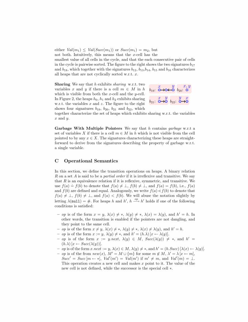
Sharing We say that h exhibits sharing w.r.t. twovariables x and y if there is a cell m ∈ M in hwhich is visible from both the x-cell and the y-cell.In Figure 2, the heaps h0, h1 and h2 exhibits sharingw.r.t. the variables x and z. The figure to the rightshows four signatures b19, b20, b21 and b22, whichtogether characterize the set of heaps which exhibits sharing w.r.t. the variablesx and y.

Garbage With Multiple Pointers We say that h contains garbage w.r.t aset of variables X if there is a cell m ∈M in h which is not visible from the cellpointed to by any x ∈ X. The signatures characterizing these heaps are straight-forward to derive from the signatures describing the property of garbage w.r.t.a single variable.

C Operational Semantics

In this section, we define the transition operations on heaps. A binary relationR on a set A is said to be a partial order if it is irreflexive and transitive. We saythat R is an equivalence relation if it is reflexive, symmetric, and transitive. Weuse f(a) .= f(b) to denote that f(a) 6= ⊥, f(b) 6= ⊥, and f(a) = f(b), i.e., f(a)and f(b) are defined and equal. Analogously, we write f(a)lf(b) to denote thatf(a) 6= ⊥, f(b) 6= ⊥, and f(a) < f(b). We will abuse the notation slightly byletting λ(null) = #. For heaps h and h′, h

op−→ h′ holds if one of the followingconditions is satisfied:

– op is of the form x = y, λ(x) 6= ∗, λ(y) 6= ∗, λ(x) = λ(y), and h′ = h. Inother words, the transition is enabled if the pointers are not dangling, andthey point to the same cell.

– op is of the form x 6= y, λ(x) 6= ∗, λ(y) 6= ∗, λ(x) 6= λ(y), and h′ = h.– op is of the form x := y, λ(y) 6= ∗, and h′ = (h.λ) [x← λ(y)].– op is of the form x := y.next , λ(y) ∈ M , Succ(λ(y)) 6= ∗, and h′ =

(h.λ) [x← Succ(λ(y))].– op is of the form x.next := y, λ(x) ∈M , λ(y) 6= ∗, and h′ = (h.Succ) [λ(x)← λ(y)].– op is of the from new(x), M ′ = M ∪ {m} for some m 6∈M , λ′ = λ [x← m],

Succ′ = Succ [m← ∗], Val ′(m′) = Val(m′) if m′ 6= m, and Val ′(m) = ⊥.This operation creates a new cell and makes x point to it. The value of thenew cell is not defined, while the successor is the special cell ∗.

– op is of the form delete(x), λ(x) ∈ M , and h′ = h λ(x). The operationdeletes the x-cell.

– op is of the form read(x ), λ(x) ∈M , and h′ = (h.Val) [λ(x)← i ], where i isthe value assigned to x-cell.

– op is of the form x.num = y.num, λ(x) ∈ M , λ(y) ∈ M , Val(λ(x)) .=Val(λ(y)), and h′ = h. The transition is enabled if the pointers are notdangling and the values of their cells are defined and equal.

– op is of the form x.num < y.num, λ(x) ∈ M , λ(y) ∈ M , Val(λ(x)) lVal(λ(y)), and h′ = h.

– op is of the form x.num := y.num, λ(x) ∈ M , λ(y) ∈ M , Val(λ(y)) 6= ⊥,and h′ = (h.Val) [λ(x)← Val(λ(y))].

– op is of the form x.num :> y.num, λ(x) ∈M , λ(y) ∈M , Val(λ(y)) 6= ⊥, andh′ = (h.Val) [λ(x)← i], where i > Val(λ(y)). The case for x.num :< y.numis defined analogously.

D Operations on Signatures

In this section, a number of operations on signatures are defined. A signature gis said to be saturated if (i) ≡ is an equivalence relation; (ii) ≺ is a partial order;(iii) m1 ≡ m2 m2 ≺ m3 implies m1 ≺ m3; and (iv) m3 ≺ m1 and m1 ≡ m2

implies m3 ≺ m2. For a signature g = (M,Succ, λ,Ord), we define its saturation,denoted sat (g), to be the signature

(M,Succ, λ,Ord ′

)where Ord ′ ⊇ Ord is the

smallest set sufficient for making g saturated. We use M# to denote M ∪ {#}.Assume a saturated signature g = (M,Succ, λ,Ord).Operations on cells. For m 6∈ M , we define g ⊕m to be the signature g′ =(M ′,Succ′, λ′,Ord ′

)such that M ′ = M ∪ {m}, Succ′ = Succ, λ′ = λ, and

Ord ′ = Ord . i.e. we add a new cell to g. Observe that the added cell is thenisolated.

We define g ⊕ λ(x) to be the signature g′ =(M ′,Succ′, λ′,Ord ′

)such that

M ′ = M ∪ {m}, Succ′ = Succ, λ′ = λ [x← m], and Ord ′ = Ord . i.e. we add anew cell to g which is pointed by x .

For m ∈ M , we define g m to be the signature g′ =(M ′,Succ′, λ′,Ord ′

)such that

– M ′ = M − {m}.– Succ′(m′) = Succ(m′) if Succ(m′) 6= m, and Succ′(m′) = ∗ otherwise.– λ′(x) = ∗ if λ(x) = m, and λ′(x) = λ(x) otherwise.– Ord ′(m1,m2) = Ord(m1,m2) if m1,m2 ∈M ′.

Operations on variables. We use g⊕ x to denote the set of signatures we getfrom g by letting x point anywhere inside g, except on ∗. Formally, we defineg ⊕ x to be the smallest set containing each signature g′ such that one of thefollowing conditions is satisfied:

1. There is a cell m ∈M#, and g′ = (g.λ) [x← m].2. There is a cell m 6∈ M , and a signature g1 such that g1 = g ⊕ m, g′ =

(g1.λ) [x← m].

3. There are m1 ∈M , m2 6∈M , and signatures g1, g2, g3 such that Succ(m1) 6=⊥, g1 = g⊕m2, g2 = (g1.Succ) [m2 ← Succ(m1)], g3 = (g2.Succ) [m1 ← m2],and g′ = (g3.λ) [x← m2].

For variables x and y, λ(x) ∈M#, we use g⊕=x y to denote (g.λ) [y ← λ(x)],i.e. we make y point to the same cell as x. Furthermore, we define g ⊕ 6=x yto be the smallest set containing each signature g′ such that g′ ∈ (g ⊕ y), andλ′(y) 6= λ′(x), i.e. we make y point anywhere inside g except on x-cell and ∗. As aspecial case, we use g⊕ 6=# y to denote the smallest set containing each signatureg′ such that g′ ∈ (g ⊕ y), and λ′(y) 6= #, i.e. we make y point anywhere insideg except on # and ∗.

For variables x and y, λ(x) ∈M , Succ(λ(x)) ∈M#, we use g⊕x→y to denotethe set of signatures we get from g by letting y point to the successor of x-cell.Formally, we define g ⊕x→ y to be the smallest set containing each signature g′

such that one of the following conditions is satisfied:

1. g′ = (g.λ) [y ← Succ(λ(x))].2. There is a cell m 6∈ M , and signatures g1, g2, g3, such that g1 = g ⊕m, g2 = (g1.Succ) [m← Succ1(λ(x)], g3 = (g2.Succ) [λ(x)← m], and g′ =(g3.λ) [y ← m].

for variables x and y, Succ(λ(x)) = ∗, we use g⊕x→∗y to denote the signaturewe get from g by letting y point to the new added cell in between x-cell and∗. Formally, we define g ⊕x→∗ y to be the signature g′ such that there is a cellm 6∈M , and signatures g1, g2, g3, such that g1 = g⊕m, g2 = (g1.Succ) [m← ∗],g3 = (g2.Succ) [λ(x)← m], and g′ = (g3.λ) [y ← m].

For variables x and y, λ(x) ∈ M#, we use g ⊕x← y to denote the set ofsignatures we get from g by letting y point to any cell except ∗, where it has nosuccessor or its successor is x-cell. Formally, we define g⊕x← y to be the smallestset containing each signature g′ such that one of the following conditions issatisfied:

1. There is a cell m ∈ M such that Succ(m) = ⊥ or Succ(m) = λ(x), andg′ = (g.λ) [y ← m].

2. There is a cell m 6∈ M , and a signature g1 such that g1 = g ⊕ m, g′ =(g1.λ) [y ← m].

3. There are m1 ∈M , m2 6∈M , and signatures g1, g2, g3, such that Succ(m1) =λ(x), g1 = g ⊕m2, g2 = (g1.Succ) [m2 ← λ(x)], g3 = (g2.Succ) [m1 ← m2],and g′ = (g3.λ) [y ← m2].

For variables x and y, λ(x) ∈M , we use g⊕≡xy to denote the set of signatureswe get from g by letting y point to any cell such that possibly λ(y) ≡ λ(x).Formally, we define g ⊕≡x y to be the smallest set containing each signature g′

such that one of the following conditions is satisfied:

1. There is a cell m ∈ M such that Ord(m,λ(x)) =≡ or Ord(m,λ(x)) = ⊥,and g′ = (g.λ) [x← m].

2. There is a cell m 6∈ M , and a signature g1 such that g1 = g ⊕ m, g′ =(g1.λ) [x← m].

3. There are m1 ∈M , m2 6∈M , and signatures g1, g2, g3 such that Succ(m1) 6=⊥, g1 = g⊕m2, g2 = (g1.Succ) [m2 ← Succ(m1)], g3 = (g2.Succ) [m1 ← m2],and g′ = (g3.λ) [x← m2].

For variables x and y, λ(x) ∈M , we use g⊕≺xy to denote the set of signatureswe get from g by letting y point to any cell such that possibly λ(y) ≺ λ(x).Formally, we define g ⊕≺x y to be the smallest set containing each signature g′

such that one of the following conditions is satisfied:

1. There is a cell m ∈ M such that Ord(m,λ(x)) =≺, or Ord(m,λ(x)) = ⊥,and g′ = (g.λ) [x← m].

2. There is a cell m 6∈ M , and a signature g1 such that g1 = g ⊕ m, g′ =(g1.λ) [x← m].

3. There are m1 ∈M , m2 6∈M , and signatures g1, g2, g3 such that Succ(m1) 6=⊥, g1 = g⊕m2, g2 = (g1.Succ) [m2 ← Succ(m1)], g3 = (g2.Succ) [m1 ← m2],and g′ = (g3.λ) [x← m2].

For variables x and y, λ(x) ∈M , we use g⊕x≺y to denote the set of signatureswe get from g by letting y point to any cell such that possibly λ(x) ≺ λ(y).Formally, we define g ⊕x≺ y to be the smallest set containing each signature g′

such that one of the following conditions is satisfied:

1. There is a cell m ∈ M such that Ord(λ(x),m) =≺, or Ord(λ(x),m) = ⊥,and g′ = (g.λ) [x← m].

2. There is am 6∈M , and a signature g1 such that g1 = g⊕m, g′ = (g1.λ) [x← m].3. There are m1 ∈M , m2 6∈M , and signatures g1, g2, g3 such that Succ(m1) 6=⊥, g1 = g⊕m2, g2 = (g1.Succ) [m2 ← Succ(m1)], g3 = (g2.Succ) [m1 ← m2],and g′ = (g3.λ) [x← m2].

For a variable x, we use g x to denote g′ = (g.λ) [x← ⊥], i.e. we remove xfrom g.Operations on edges. For variables x and y, λ(x) ∈ M , λ(y) ∈ M#, we useg � (x → y) to denote (g.Succ) [λ(x)← λ(y)], i.e. we remove the edge betweenx-cell and its successor (if any), and add an edge from x-cell to y-cell.

For a variable x, λ(x) ∈M , we use g� (x→) to denote the set of signatureswe get from g by making an edge from x-cell to anywhere inside g, except ∗.Formally, we define g � (x →) to be the smallest set containing each signatureg′ such that one of the following conditions is satisfied:

1. There is a m ∈M#, and g′ = (g.Succ) [λ(x)← m].2. There is a m 6∈M such that g′ = ((g ⊕m).Succ) [λ(x)← m].3. There are m1 ∈M , m2 6∈M , and signatures g1, g2, g3, such that Succ(m1) 6=⊥, g1 = g⊕m2, g2 = (g1.Succ) [m2 ← Succ1(m1)], g3 = (g2.Succ) [m1 ← m2],and g′ = (g3.Succ) [λ3(x)← m2].

We use ML to denote the set of cells such that for all m ∈ML, Succ(m) = ∗.For a variable x, λ(x) ∈ M , we define g � (ML → x) to be the smallest setcontaining each signature g′ such that g′ = (g.Succ) [m′ ← λ(x)], where m′ ∈

M l, M l ∈ P(M L), and P(M L) is the power set of ML. i.e. we get each g′ bypicking some cells in ML, and make their successors all point to x .

For a variable x, λ(x) ∈M , we use g� (x→) to denote (g.Succ) [λ(x)← ⊥],i.e. we remove the edge from x-cell and its successor (if any).Operation on ordering relations. For variables x and y, λ(x) ∈M , λ(y) ∈M ,we use g�(x ≡ y) to denote (g.Ord) [(λ(x), λ(y))←≡], (g.Ord) [(m1, λ(y))←≡],for m1 ∈ M , Ord(m1, λ(x)) =≡, and (g.Ord) [(m2, λ(x))←≡], for m2 ∈ M ,Ord(m2, λ(y)) =≡, i.e. we make the ordering relation between x-cell and y-cellequal to ≡, and make g′ saturated.

For variables x and y, λ(x) ∈ M , λ(y) ∈ M , we use g � (x ≺ y) to denote(g.Ord) [(λ(x), λ(y))←≺], (g.Ord) [(m1, λ(y))←≺], form1 ∈M , Ord(m1, λ(x)) =≡or Ord(m1, λ(x)) =≺, and (g.Ord) [(λ(x),m2)←≺], form2 ∈M , Ord(λ(y),m2) =≡or Ord(λ(y),m2) =≺, i.e. we make the ordering relation between x-cell and y-cellequal to ≺, and make g′ saturated.

For a variable x, λ(x) ∈ M , we use g �Ord λ(x) to denote that for all m ∈M − {λ(x)}, (g.Ord) [(λ(x),m)← ⊥], (g.Ord) [(m,λ(x))← ⊥], i.e. we removethe ordering relation between x-cell and other cells.

E Computing Predecessors

In this section, we define how to compute predecessors of a saturated signature.We assume a saturated signature g = (M,Succ, λ,Ord).

We define Pre(g)(x = y) to be the set of saturated signatures g′ such thatone of the following conditions is satisfied:

– λ(x) ∈M#, λ(y) ∈M#, λ(x) = λ(y) and g′ = g.– λ(x) ∈M#, λ(y) = ⊥, and g′ = g ⊕=x y.– λ(x) = ⊥, λ(y) ∈M#, and g′ = g ⊕=y x.– λ(x) = ⊥, λ(y) = ⊥, and there is a signature g1 such that g1 ∈ g ⊕ x,g′ = g1 ⊕=x y.

We define Pre(g)(x 6= y) to be the set of saturated signatures g′ such thatone of the following conditions is satisfied:

– λ(x) ∈M#, λ(y) ∈M#, λ(x) 6= λ(y) and g′ = g.– λ(x) ∈M#, λ(y) = ⊥, and g′ ∈ g ⊕6=x y.– λ(x) = ⊥, λ(y) ∈M#, and g′ ∈ g ⊕6=y x.– λ(x) = ⊥, λ(y) = ⊥, and there is a signature g1 such that g1 ∈ g ⊕ x,g′ ∈ g1 ⊕6=x y.

We define Pre(g)(x := y) to be the set of saturated signatures g′ such thatone of the following conditions is satisfied:

– λ(x) ∈M#, λ(y) ∈M#, λ(x) = λ(y) and g′ = g x.– λ(x) ∈ M#, λ(y) = ⊥, and there is a signature g1 such that g1 = g ⊕=x y,g′ = g1 x.

– λ(x) = ⊥, λ(y) ∈M#, and g′ = g.

– λ(x) = ⊥, λ(y) = ⊥, and g′ ∈ g ⊕ y.

We define Pre(g)(x := y.next)) to be the set of saturated signatures g′ suchthat one of the following conditions is satisfied:

– λ(x) ∈M#, λ(y) ∈M , Succ(λ(y)) = λ(x), and g′ = g x.– λ(x) ∈ M#, λ(y) ∈ M , Succ(λ(y)) = ⊥, and there is a signature g1 such

that g1 = g � (y → x), g′ = g1 x.– λ(x) ∈M#, λ(y) = ⊥, and there are signatures g1, g2 such that g1 ∈ g⊕x←y,g2 = g1 � (y → x), g′ = g2 x.

– λ(x) = ⊥, λ(y) ∈M , Succ(λ(y)) ∈M#, and g′ = g.– λ(x) = ⊥, λ(y) ∈ M , Succ(λ(y)) = ∗, and there is a signature g1 such thatg1 = g ⊕y→∗ x, g′ = g1 x.

– λ(x) = ⊥, λ(y) ∈M , Succ(λ(y)) = ⊥, and g′ ∈ g � (y →).– λ(x) = ⊥, λ(y) = ⊥, and there are signatures g1, g2, g3 such that g1 ∈ g⊕ x,g2 ∈ g1 ⊕x← y, g3 = g2 � (y → x), g′ = g3 x.

We define Pre(g)(x.next := y) to be the set of saturated signatures g′ suchthat one of the following conditions is satisfied:

– λ(x) ∈M , λ(y) ∈M#, Succ(λ(x)) = λ(y), and g′ = g � (x→).– λ(x) ∈ M , Succ(λ(x)) ∈ M#, λ(y) = ⊥, and there is a signature g1 such

that g1 ∈ g ⊕x→ y, g′ = g1 � (x→).– λ(x) ∈M , Succ(λ(x)) = ⊥, λ(y) ∈M#, and g′ = g.– λ(x) ∈M , Succ(λ(x)) = ⊥, λ(y) = ⊥, and g′ ∈ g ⊕ y.– λ(x) = ⊥, λ(y) ∈ M#, and there is signature g1 such that g1 ∈ g ⊕y← x,g′ = g1 � (x→).

– λ(x) = ⊥, λ(y) = ⊥, and there are signatures g1, g2 such that g1 ∈ g ⊕ y,g2 ∈ g1 ⊕y← x, g′ = g2 � (x→).

We define Pre(g)(new(x)) to be the set of saturated signatures g′ such thatone of the following conditions is satisfied:

– λ(x) is x-semi-isolated, and there is signature g1 such that g1 = g λ(x)and g′ = g1 x.

– λ(x) = ⊥ and g′ = g or g′ ∈ g m for some semi-isolated cell m.

We define Pre(g)(delete(x)) to be the set of saturated signatures g′ such thatone of the following conditions is satisfied:

– λ(x) = ∗, and there are a signature g1, g2 such that g1 = gx, g2 = g1⊕λ(x),g′ = g2 � (ML → x).

– λ(x) = ⊥, and there is signatures g1 such that g1 = g ⊕ λ(x), g′ = g1 �(ML → x).

We define Pre(g)(read(x )) to be the set of saturated signatures g′ such thatone of the following conditions is satisfied:

– λ(x) ∈M , and g′ = g �Ord λ(x).

– λ(x) = ⊥, and there is a signature g1 such that g1 ∈ g ⊕ 6=# x, g′ = g1 �Ord

λ(x)

We define Pre(g)(x.num = y.num) to be the set of saturated signatures g′

such that one of the following conditions is satisfied:

– λ(x) ∈M , λ(y) ∈M , λ(x) ≡ λ(y), and g′ = g.– λ(x) ∈M , λ(y) ∈M , Ord(x, y) = ⊥, and g′ = g � (x ≡ y).– λ(x) ∈ M , λ(y) = ⊥, there is signature g1 such that g1 ∈ g ⊕≡x y, g′ =g1 � (x ≡ y).

– λ(x) = ⊥, λ(y) ∈ M , there is signature g1 such that g1 ∈ g ⊕≡y x, g′ =g1 � (x ≡ y).

– λ(x) = ⊥, λ(y) = ⊥, there are signatures g1, g2 such that g1 ∈ g ⊕6=# y,g2 ∈ g1 ⊕≡y x, g′ = g2 � (x ≡ y).

We define Pre(g)(x.num < y.num) to be the set of saturated signatures g′

such that one of the following conditions is satisfied:

– λ(x) ∈M , λ(y) ∈M , λ(x) ≺ λ(y), and g′ = g.– λ(x) ∈M , λ(y) ∈M , Ord(x, y) = ⊥, and g′ = g � (x ≺ y).– λ(x) ∈ M , λ(y) = ⊥, there is a signature g1 such that g1 ∈ g ⊕x≺ y,g′ = g1 � (x ≺ y).

– λ(x) = ⊥, λ(y) ∈ M , there is signature g1 such that g1 ∈ g ⊕≺y x, g′ =g1 � (x ≺ y).

– λ(x) = ⊥, λ(y) = ⊥, there are signatures g1, g2 such that g1 ∈ g ⊕6=# y,g2 ∈ g1 ⊕≺y x, g′ = g2 � (x ≺ y).

We define Pre(g)(x.num := y.num) to be the set of saturated signatures g′

such that one of the following conditions is satisfied:

– λ(x) ∈M , λ(y) ∈M , λ(x) ≡ λ(y), and g′ = g �Ord λ(x).– λ(x) ∈M , λ(y) ∈M , Ord(x, y) = ⊥, and g′ = g �Ord λ(x).– λ(x) ∈ M , λ(y) = ⊥, and there is a signature g1 such that g1 ∈ g ⊕≡x y,g′ = g1 �Ord λ(x).

– λ(x) = ⊥, λ(y) ∈M , and g′ = g.– λ(x) = ⊥, λ(y) = ⊥, and g′ ∈ g ⊕ 6=# y.

We define Pre(g)(x.num :< y.num) to be the set of saturated signatures g′

such that one of the following conditions is satisfied:

– λ(x) ∈M , λ(y) ∈M , λ(x) ≺ λ(y), and g′ = g �Ord λ(x).– λ(x) ∈M , λ(y) ∈M , Ord(x, y) = ⊥, and g′ = g �Ord λ(x).– λ(x) ∈ M , λ(y) = ⊥, and there is a signature g1 such that g1 ∈ g ⊕x≺ y,g′ = g1 �Ord λ(x).

– λ(x) = ⊥, λ(y) ∈M , and g′ = g.– λ(x) = ⊥, λ(y) = ⊥, and g′ ∈ g ⊕6=# y.

We define Pre(g)(x.num :> y.num) to be the set of saturated signatures g′

such that one of the following conditions is satisfied:

– λ(x) ∈M , λ(y) ∈M , λ(y) ≺ λ(x), and g′ = g �Ord λ(x).– λ(x) ∈M , λ(y) ∈M , Ord(x, y) = ⊥, and g′ = g �Ord λ(x).– λ(x) ∈ M , λ(y) = ⊥, and there is a signature g1 such that g1 ∈ g ⊕≺x y,g′ = g1 �Ord λ(x).

– λ(x) = ⊥, λ(y) ∈M , and g′ = g.– λ(x) = ⊥, λ(y) = ⊥, and g′ ∈ g ⊕ 6=# y.