Automatic urban road network extraction from massive GPS trajectories of taxis

Song Gao1, Mingxiao Li1,2, Jinmeng Rao1, Gengchen Mai3, Timothy Prestby1, Joseph Marks1, Yingjie Hu4

1. GeoDS Lab, Department of Geography, University of Wisconsin-Madison, Madison, WI 53706, USA; 2. State Key Laboratory of Resources and Environmental Information System, Institute of Geographic

Sciences and Natural Resources Research, Chinese Academy of Sciences, Beijing 100101, China; 3. STKO Lab, Department of Geography, University of California, Santa Barbara, CA 93106, USA;

4. GeoAI Lab, Department of Geography, University at Buffalo, Buffalo, NY 14260, USA.

Abstract:

Urban road networks are fundamental transportation infrastructures in daily life and essential in digital maps to support vehicle routing and navigation. Traditional methods of map vector data generation based on surveyor’s field work and map digitalization are costly and have a long update period. In the Big Data age, large-scale GPS-enabled taxi trajectories and high-volume ride-sharing datasets become increasingly available. These datasets provide high-resolution spatiotemporal information about urban traffic along road networks. In this study, we present a novel geospatial-big-data-driven framework that includes trajectory compression, clustering, and vectorization to automatically generate urban road geometric information. A case study is conducted using a large-scale DiDi ride-sharing GPS dataset in the city of Chengdu in China. We compare the results of our automatic extraction method with the road layer downloaded from OpenStreetMap. We measure the quality and demonstrate the effectiveness of our road extraction method regarding accuracy, spatial coverage and connectivity. The proposed framework shows a good potential to update fundamental road transportation information for smart-city development and intelligent transportation management using geospatial big data.

1 Introduction

Increasingly, mobile Internet, ubiquitous sensors (Hancke & Hancke Jr. 2013) and growing Volunteering Geographic Information (VGI) (Goodchild 2007) altogether boost the construction of transportation information infrastructures (Shaw 2010). Urban road networks, as the important carriers of transportation in cities, provide basic support for human & goods transportation and various Location-Based Services (LBS) such as vehicle route planning and navigation, which are the keys to smart transportation. However, how to build and update the road network in a rapid and cost-effective way still remains to be a challenging problem.

Traditional methods such as field surveying and map digitalization are usually costly and cannot produce up-to-date urban road networks in time (Tao 2000). With the rapid development of information and communication technologies (ICTs) and positioning technologies such as the Global Positioning System (GPS), huge amounts of vehicle movement trajectory data have been

accumulated (Liu et al. 2012). By leveraging these massive GPS trajectories, automatic construction and updates to road networks can be achieved in near real-time (Li et al. 2012). Although the idea for the extraction of urban road networks from GPS trajectory data is intuitive, there is still a considerable gap between the raw GPS traces and the road network structure. On the one hand, the GPS trajectories have non-negligible errors due to the inherent noise in GPS, which makes it difficult to distinguish two closely located road segments in some cases (Cao and Krumm 2009). On the other hand, complex urban environment such as “urban canyon” often leads to the deterioration in the GPS precision, making the trajectories less accurate to represent the road segments. In addition, the diversity and complexity of the road network structure in some places (e.g., roundabouts, parking lots) also cause challenges for road network extraction from raw GPS trajectories. Besides the GPS precision and the complex road network structure, the preprocessing of trajectory data is another challenge. A large proportion of the GPS data on straight road segments are redundant since fewer points are already enough to reconstruct the linear road segments, whereas the curved roads required more points. Also, when there is traffic congestion, more redundant data (e.g., stay points) will be produced (Zheng 2015). These situations may cause high computational costs and limit the road network extraction efficiency. In addition, trajectory outliers (i.e., anomalies) will make it non-trivial to reconstruct the road network and need to be addressed during the preprocessing step (Zheng 2015; Wang et al. 2019).

To this end, in this chapter, we focus on the trajectory sampling, compression, and clustering techniques to update road geometry information with regards to the spatial coverage and topological connectivity. We conduct a literature review in the following section and then propose a geospatial-big-data-driven framework to achieve an automatic road network extraction. Specifically, we first introduce a trajectory compression approach to reduce redundant trajectory data to avoid the unnecessary computational cost. Then we present an anisotropic density-based trajectory clustering with noise (ADCN) algorithm (Mai et al. 2018) for identifying the trajectory points on the road segments, and finally a kernel density estimation and vectorization approach is utilized for road network extraction.

2 Literature Review

Existing literature on road network extraction methods can be classified into two categories: density-based approaches and cluster-based approaches.

2.1 Density-based approaches

The first category mainly relies on density estimation and raster processing techniques. It converts trajectory data into raster data based on density and extracts the road network using morphological methods (Davies and Beresford 2006; Wu et al. 2007; Shi et al 2009; Zhao et al. 2011; Biagioni and Eriksson 2012; Jiang et al. 2012; Wang et al. 2015; Kuntzsch et al. 2016; Tang et al. 2017). For example, Davies and Beresford (2006) first generated a 2D histogram based on the GPS trajectories, then applied a global density threshold on the cells to find potential road areas, and finally computed road centerlines based on the Voronoi graph. Shi et al. (2009) converted vehicle GPS trajectories into a road network bitmap, then compute the road network skeleton on the bitmap, and finally extract the vector road network map data from the skeleton. Biagioni and

Eriksson (2012) generated road network skeleton based on a kernel-density method and use a map-matching method to achieve topology reconstruction. Kuntzsch et al. (2016) formulated an explicit intersection model which integrated consistency measurements with the raw trajectory data to better perform geometry and topology reconstruction of the network; Tang et al. (2017) employed Delaunay triangulation with the trajectory stream fusion to improve the map generation accuracy. However, the difference in trajectory density has a great influence on the extraction effect, which could make these methods unreliable in cases with heterogenous trajectory density.

2.2 Cluster-based approaches

The second category adopted clustering methods to generate road networks (Edelkamp et al. 2003; Lee et al. 2007; Worrall et al. 2007; Cao and Krumm 2009; Wang et al. 2015; Aronov et al. 2016; Stanojevic et al. 2018). Trajectory clustering is usually used to find representative trajectories shared by different objects such as individuals or vehicles (Zheng 2015). For example, Gaffney and Smyth (1999) and Cadez et al. (2000) used a regression mixture model and an Expectation-Maximization (EM) model to cluster trajectories according to the overall distance between two trajectories. Lee et al. (2007) proposed TRACLUS, a modified density-based trajectory clustering algorithm for grouping close trajectory line segments into clusters, which is based on the original point-based DBSCAN algorithm. Li et al. (2010) further introduced an incremental clustering algorithm that reduces the computational and storage cost. In practice, trajectory clustering can be naturally used for road network extraction. Edelkamp et al. (2003) applied the K-means algorithm to cluster the trajectories and then fit the road centerline with the spline curve. This approach is suitable for data with small density difference, low noise, and high frequency sampling. Worrall et al. (2007) used clustering to extract the skeleton points of the road network and used the least squares regression method to connect the skeleton points to generate the road network. Cao and Krumm (2009) clarified the GPS traces using simulations of physical forces among the traces, and then merged the clarified traces into a graph representation of the road network structure. Wang et al. (2015) determined a proper circle boundary to cluster trajectory data into intersections and used the core points to build the road networks. Stanojevic et al. (2018) formulated the road network generation task as a network alignment optimization task and proposed an offline algorithm that clustered GPS points for graph construction as well as an online algorithm that can create and update the road network. However, the trajectory points on the road networks include linear features with a continuously changing density which makes current clustering methods tend to either create an increasing number of small clusters or add noise points into large clusters. Therefore, incorporating directional information into clustering methods has become an efficient way to cluster anisotropic distributed points and enhance extraction performance (Mai et al. 2018).

3 Methodology

In this section, we present the details of our road map generation method using GPS trajectories. As shown in Figure 1, the trajectory big data processing workflow can be divided into the following steps. First, we utilized a trajectory compression approach to simplify the trajectory data and reduce unnecessary computational cost. Second, we applied the Anisotropic Density-based Clustering with Noise (ADCN) algorithm (Mai et al. 2018) to identify the trajectory points

that were along the road networks with high confidence. Third, a kernel density estimation (KDE) approach was used to generate a continuous surface. Fourth, high-density areas were selected as candidates to further extract the road centerlines using thinning and vectorization operators. Finally, the extracted road network connectivity should be evaluated.

Figure 1. The trajectory big data processing workflow in this study.

3.1 Trajectory compression

With the rapid development of ICT technologies and positioning devices, the spatiotemporal resolution of trajectory data has unprecedentedly increased. However, large amount of trajectory data lead to high computational costs and a large storage space is necessary to support the data processing and management. With regards to road network extraction, it is straightforward to reconstruct the road segments as long as the trajectory points at the intersections can be obtained and then connected. Thus, a trajectory compression method was applied to simplify the trajectory data points and improve extraction efficiency.

The main purpose of trajectory compression in road network extraction is to maintain the shape of the trajectories. Several popular algorithms for line simplification include Douglas-Peucker algorithm (Douglas & Peucker 1973), Reumann-Witkam algorithm (Reumann & Witkam 1974), Lang simplification (Lang 1969), Opheim simplification (Opheim 1982), etc. The evaluation and comparison of these line simplification algorithms for vector generalization were conducted by Shi & Cheung (2006). McMaster (1989) proposed a conceptual model including a sequential set of five procedures for processing linear data with focuses on geometric simplification and smoothing. In our method, we applied the widely used DP algorithm for trajectory simplification. A graphic illustration of the DP algorithm is shown in Figure 2. To simplify the trajectory, we first mark the first point and the last point as endpoints and added them to the reserved point set. Then, the point that is furthest from the line segment with the endpoints is found, and the distance between the point and the line segment is calculated. If the distance is larger than a compression threshold α, the point is marked as an endpoint and added to the reserved point set (e.g. P4 in in Figure 2(b) and P5 in Figure 2(c)). Otherwise, the points between the endpoints would be discarded (e.g. P2 and P3 in Figure 2(c)). The same process is iteratively performed until all the trajectory points are marked as an endpoint or discarded (Figure 2(d)). Finally, the points in the reserved point set are sorted according to the original trajectory sequence and linked to generate the compressed trajectory.

Figure 2. Illustration of the Douglas-Peucker trajectory compression algorithm.

3.2 Identification of the trajectory points along the road

Density-based clustering algorithms such as DBSCAN have been widely used for spatial knowledge discovery such as the detection of urban areas of interest (Hu et al. 2015) and vague cognitive regions (Gao et al. 2017). The DBSCAN algorithm offers several key advantages compared with other clustering algorithms such as K-Means. DBSCAN can discover clusters with arbitrary shapes, are robust to noise, and do not require prior knowledge (Ester et al. 1996). However, the trajectory points demonstrate clear anisotropic spatial processes, which makes these methods tend to either create an increasing number of small clusters or add noise points into large clusters. Therefore, in this section, we apply a novel anisotropic density-based clustering algorithm with noise (ADCN) (Mai et al. 2018) to cluster anisotropic points for identifying the trajectory points along the roads1.

3.2.1 Density-based spatial clustering of applications with noise (DBSCAN)

The used ADCN algorithm was modified based on the DBSCAN algorithm. Thus, before we describe the ADCN algorithm in detail, we first introduce some fundamental concepts of the DBSCAN algorithm (Ester et al. 1996). The key idea of the DBSCAN algorithm is that: given a set of points, it groups nearby points (i.e., the points in high-density areas) together and marks the points in low-density areas as outliers. In order to group the points based on the density, the Eps-neighborhood of a point is defined (see Definition 1).

1 The Python implementation of the ADCN algorithm can be found at: https://github.com/gissong/ADCN

(a) Original trajectory

P1

P2P3

P4

P5

P6

(c) Addition of P5

(b) Addition of P4

(d) Compressed trajectory

P1

P2P3

P4

P5

P6

P1

P2P3

P4

P5

P6 P1

P2P3

P4

P5

P6

Definition 1 (Eps-neighborhood of a point): The Eps-neighborhood 𝑁"#$(𝑝') of point 𝑝' in a dataset D is defined as all the points within the scan circle centered at 𝑝' with a radius Eps, which is expressed as follows:

𝑁"#$(𝑝') = {𝑝+(𝑥+, 𝑦+) ∈ 𝐷|𝑑𝑖𝑠𝑡(𝑝', 𝑝+) ≤ 𝐸𝑝𝑠}

where 𝑑𝑖𝑠𝑡(𝑝', 𝑝+) is the distance between point 𝑝' and point 𝑝+.

There are two kinds of points in a cluster: core points (i.e., points inside of the cluster) and border points (i.e., points on the border of the cluster). One intuition is that for each point of a cluster, an Eps-neighborhood should contain at least a minimum number of points (MinPts). However, an Eps-neighborhood of a border point usually contains much fewer points than an Eps-neighborhood of a core point, and it is hard to choose the representative MinPts for all points. Thus, DBSCAN introduces three basic concepts: directly density-reachable, density-reachable and density-connected (see Definition 2-4).

Definition 2 (directly density-reachable): A point 𝑝 is directly density-reachable from a point 𝑞 wrt. Eps and MinPts if:

1. p ∈ 𝑁"#$(q) and

2. |𝑁"#$(q)| ≥ 𝑀𝑖𝑛𝑃𝑡𝑠 (core point condition).

Definition 3 (density-reachable): A point 𝑝 is density-reachable from a point 𝑞 wrt. Eps and MinPts if there is a chain of points 𝑝@, … , 𝑝B, 𝑝@ = 𝑞, 𝑝B = 𝑝 such that 𝑝'C@ is directly density-reachable from 𝑝'.

Definition 4 (density-connected): A point 𝑝 is density-connected to a point 𝑞 wrt. Eps and MinPts if there is a point 𝑂 such that 𝑝 and 𝑞 are density-reachable from 𝑂 wrt. Eps and MinPts.

Figure 2 illustrates core points, border points, density-reachability and density-connectivity in DBSCAN. These definitions can be used to further define the density-based notion of a cluster or a noise in DBSCAN. Specifically, the core points and border points are grouped into clustered points while the points that don’t belong to any cluster are the noise points (as shown in Figure 3).

Figure 3. Illustration of core points, border points, density-reachability and density-connectivity in the

DBSCAN algorithm.

Figure 4. Illustration of core points, border points, and noise points in the DBSCAN algorithm.

3.2.2 Anisotropic perspective on local point density

One key consideration in the ADCN algorithm is the anisotropic perspective on local point density in different directions. Without predefined direction information from spatial point datasets, one has to compute the local major direction for each point based on the spatial distribution of

neighboring points. The standard deviation ellipse (SDE) (Yuill, 1971) is a suitable method to get the major direction of a point set. Given n points, the SDE constructs an ellipse to represent the orientation and arrangement of these points. The center of this ellipse is defined as the geometric center of these n points and is calculated as:

𝑋F = ∑ 𝑥'B'H@ 𝑛I ,𝑌F = ∑ 𝑦'B

'H@ 𝑛I

The coordinates (𝑥',𝑦') of each point are normalized to the deviation from the mean center point:

𝑥LM = 𝑥' − 𝑋F, 𝑦LM = 𝑦' − 𝑌F

Thus, the semi-major axes 𝜎P and the semi-minor axes 𝜎Q of SDE are calculated as:

𝜎P = R∑ (B'H@ 𝑥LM cos 𝜃 + 𝑦LM sin 𝜃)Z 𝑛I , 𝜎Q = R∑ (B

'H@ 𝑦LM cos 𝜃 − 𝑥LM sin 𝜃)Z 𝑛I

where 𝜃 is the rotation angle and the SDE will be further used as the search polygon for clustering neighboring points (Mai et al. 2018).

3.2.3 Anisotropic density-based clusters with noise (ADCN) algorithm

In order to introduce an anisotropic perspective to density-based clustering algorithms, we have to revise some definitions. First, the original Eps-neighborhood of a point in a dataset D is defined by DBSCAN, as given in Definition 1. Such a scan circle results in an isotropic perspective on clustering. However, an anisotropic assumption will be more appropriate for trajectory points along the roads. Intuitively, in order to introduce the anisotropic perspective into DBSCAN, we can employ a scan ellipse instead of a circle to define the Eps-neighborhood of each point. Before that, we defined a set of points around a point to derive the scan ellipse;

Definition 5 (Search-neighborhood of a point): The kth nearest neighbor 𝐾𝑁𝑁(𝑝') of point 𝑝'. Here 𝑘 = 𝑀𝑖𝑛𝑃𝑡𝑠 and 𝐾𝑁𝑁(𝑝') does not include 𝑝' itself.

After determining the search-neighborhood of a point, it is possible to define the Eps-ellipse-neighborhood region (see Definition 6) and the Eps-ellipse-neighborhood (see Definition 7) of each point.

Definition 6 (Eps-ellipse-neighborhood region of a point): An ellipse 𝐸𝑅' is called an Eps-ellipse-neighborhood region of a point 𝑝' if:

1. Ellipse 𝐸𝑅' is centered at point 𝑝'.

2. Ellipse 𝐸𝑅' is scaled from the standard deviation ellipse 𝑆𝐷𝐸' computed from the search-neighborhood 𝑆(𝑝)' of point 𝑝'.

3. _`abc

_`dec = _`ab

_`de where 𝜎fgPh , 𝜎f'Bh , 𝜎fgP, 𝜎f'Bare the length of the semi-long and semi-short

axes of ellipse 𝐸𝑅' and ellipse 𝑆𝐷𝐸'.

4. 𝐴𝑟𝑒𝑎(𝐸𝑅') = π𝐸𝑝𝑠Z.

According to Definition 6, the Eps-ellipse-neighborhood region of a point is computed based on the search-neighborhood of a point. Each point should have a unique MinPts, as long as the search-neighborhood of the current point has at least two points for the computation of the standard deviation ellipse.

Definition 7 (Eps-ellipse-neighborhood of a point): An Eps-ellipse-neighborhood 𝐸𝑁"#$(𝑝') of point 𝑝' is defined as all the points inside the ellipse 𝐸𝑅', which can be expressed as:

𝐸𝑁"#$(𝑝') = {𝑝+(𝑥+, 𝑦+) ∈ 𝐷|no𝑦+ − 𝑦'p sin𝜃fgP + o𝑥+ − 𝑥'pcos𝜃fgPq

Z

𝑎Z +no𝑦+ − 𝑦'pcos𝜃fgP − o𝑥+ − 𝑥'p sin 𝜃fgPq

Z

𝑏Z ≤ 1}

Equipped with Definition 1 and Definitions 5-7, we can introduce the anisotropic perspective to density-based clustering algorithms. The definitions of directly density reachable, density reachable, cluster and noise in ADCN are similar to DBSCAN, which will not be repeated here. Figure 5 illustrates the related definitions for ADCN. The red point in the figure represents current center point. The blue points indicate the search-neighborhood of the corresponding center point according to Definition 5. The green ellipse and the green cross stand for the standard deviation ellipse constructed from the corresponding search-neighborhood and the center point. The red ellipse is the scale-transformed Eps-ellipse-neighborhood region according to Definition 6, whereas the dashed-line circle indicates a traditional scan circle in DBSCAN. As can be seen in Figure 5, ADCN could exclude the point to the left of the linear bridge pattern in the clustering process, whereas DBSCAN still includes it.

Figure 5. Illustration of the ADCN algorithm (Mai et al. 2018).

3.2.4 ADCN algorithm in road network extraction

The abovementioned ADCN algorithm takes the same parameters (MinPts and Eps) as the DBSCAN algorithm which must be decided before clustering. This is for good reasons, as the proper selection of DBSCAN parameters has been well studied, and ADCN can easily replace DBSCAN without any changes to established workflows.

The ADCN method starts with an arbitrary point 𝑝' in a point dataset D and discovers all the core points which are density reachable from point 𝑝' along the major direction. The result of the points in the clusters will be regarded as the trajectory points on the road. In order to take care of situations where all points of the search-neighborhood 𝑆(𝑝') of point 𝑝' are strictly on the same line, the short axis of the Eps-ellipse-neighborhood region 𝐸𝑅' becomes zero, and its long axis becomes infinity. This means that 𝐸𝑁"#$(𝑝') is reduced to a straight line. The process of constructing the Eps-ellipse-neighborhood 𝐸𝑁"#$(𝑝') of point 𝑝' becomes a point-on-line query. Furthermore, the ADCN method uses a kth nearest neighborhood of point 𝑝' as the search-neighborhood. Here, the center point 𝑝' will not be included in its kth nearest neighborhood. The runtimes of ADCN are heavily dominated by the search-neighborhood query which is executed on each point. Hence, the time complexities of ADCN, DBSCAN, and OPTICS are𝑂(𝑛Z) without a spatial index and 𝑂(𝑛𝑙𝑜𝑔𝑛)otherwise (Kolatch 2001; Mai et al. 2018).

3.3 Road network generation

3.3.1 Road density surface generation

After identifying the compressed and clustered GPS trajectory points on the roads, the kernel density estimation (KDE) is introduced to fit a smooth surface. To fit the surface, we used 30m*30m square grid cells to divide the space and calculated the trajectory point density of each cell. Let 𝑑@, 𝑑Z, . . . , 𝑑B be a given set of trajectory point densities. The kernel density estimator is defined as:

𝑓y(z) =1𝑛ℎz|𝐾(

𝑑 − 𝑑'ℎ )

B

'H@

where 𝑛 is the number of density sets, ℎ denotes the bandwidth parameter, and 𝐾 is a kernel function. The kernel surface value is highest at the location of the center and decreases with increasing distance from the center until reaching zero at the search radius. The density at each grid cell is calculated by adding the weighted values under the kernel surface where it overlays the raster cell center. The kernel function used in this work is based on the quartic kernel function (Silverman 1986) described as follows:

𝐾(z) = }3𝜋�@(1 − 𝑑�𝑑)Z𝑖𝑓𝑑�𝑑 < 1

0𝑜𝑡ℎ𝑒𝑟𝑤𝑖𝑠𝑒

Figure 6. A 3D Visualization of the selected quartic kernel function. The vertical axis represents the

derived K function value.

Figure 6 shows a 3D plot of the selected quartic kernel function. Note that there are two reasons we choose the quartic kernel function. First, the quartic kernel function’s resulted density estimates have higher differentiability properties. Second, it can be calculated more quickly than the gaussian kernel, which is suitable for massive-scale trajectory points with fine spatial resolution.

3.3.2 Collapse surface to centerline

After the previous steps, the areas whose density is above a threshold β are selected as the candidates. In this step, the main purpose is to extract the centerline of the candidate areas while keeping the road network topology. The thinning operator proposed by Yuan et al. (2012) was performed to remove certain grid cells from the candidate areas. For a given grid cell in the candidate area, whether it should be removed depends on its 8-neighboring cells. This method first divided the binary image (i.e., is a road pixel or not) into two disjointed subfields in a checkerboard pattern. Then, iterations were performed to remove redundant neighboring cells. The algorithm ensured that the connectivity of the cells was preserved when a cell was deleted. A combination of the thinning operator and the raster-to-vector operation converted the KDE surface of compressed trajectories into road centerlines. The quality measures of the extracted road networks including accuracy (correctness), coverage completeness, redundancy, and connectivity will be discussed with case study experiments in section 4.2.

4 Case Study

4.1 Data

We applied the above introduced trajectory compression and clustering workflow in the DiDi research open data “November 2016, Chengdu City Second Ring Road Regional Trajectory Data

Set”2 to extract the road information. Figure 7 shows the KDE visualization of over 1 million e-hailing trip origins and destinations and part of the extracted road geometry density map from 181,172 trip trajectories in one day. The date range of this dataset is from November 1 to November 30, 2016 and the temporal sampling resolution is about 2~5 seconds. The original data is about 50GB, and about 10GB after compression.

(a)

(b)

2 https://gaia.didichuxing.com

Figure 7. A map visualization of the case-study DiDi GPS data: (a) over 1 million trip origins and destinations per day; (b) part of the extracted road geometry density from 181,172 trip trajectories.

4.2 Experiment

4.2.1 Evaluation Metrics

In order to determine the effectiveness of our algorithm that generates big-data-driven road networks, we performed vector-based quality measures (Wiedemann et al. 1998). These quality measures were done by comparing a reference road network data layer to our extracted road network data layers (in Figure 8). To begin, the road networks were divided into small pieces of the same length. Next, a buffer was created as a zone with a consistent width that encircles each line segment for a given analysis. To determine if the extracted network roads match the reference roads, we constructed a buffer around the reference road data and determined if the portion of extracted roads inside of the buffer met our requirements. This is the correctness. Similarly, we constructed a buffer around the extracted road data and evaluated the portion of reference roads inside the buffer to further analyze the results. This is called the completeness. Together, correctness and completeness constitute a comprehensive metric known as quality. Another evaluation metric known as metric known as redundancy determines the degree of overlap in the road extraction methods.

Figure 8. The matching principle between extracted roads and reference roads using buffers.

• Completeness The completeness constitutes the percentage of reference roads delineated by the extracted road network. That is, the percentage of the reference road data located within the buffer encircling the extracted roads. The closer completeness is to 1, the better the performance of the algorithm is. Let Lmr be the length of matched reference roads and Lr be the length of all reference roads.

𝐶𝑜𝑚𝑝𝑙𝑒𝑡𝑒𝑛𝑒𝑠𝑠 =𝐿f�𝐿�

• Correctness

The correctness signifies the percentage of extracted road data that actually corresponds to the reference road. In other words, it is the percentage of the extracted road network that falls within the buffer surrounding the reference roads. The closer correctness is to 1, the better. Let Lme be the length of matched extraction roads and Le be the length of all extracted roads.

𝐶𝑜𝑟𝑟𝑒𝑐𝑡𝑛𝑒𝑠𝑠 =𝐿f�𝐿�

• Quality The quality summarizes the road extraction method by factoring both completeness and correctness into one value. The closer quality is to 1, the better. Let Lur be the length of unmatched reference roads.

𝑄𝑢𝑎𝑙𝑖𝑡𝑦 =𝐿f�

𝐿� + 𝐿��

• Redundancy

The redundancy measures the percentage of the matched extraction road network which overlaps itself. The closer redundancy is to 0, the better.

𝑅𝑒𝑑𝑢𝑛𝑑𝑎𝑛𝑐𝑦 =𝐿f� − 𝐿f�

𝐿f�

4.2.2 Results

In order to evaluate the extracted road network quality, we downloaded the OpenStreetMap (OSM) data as the reference road network layer. Moreover, we also compared our approach to the baseline approach that is directly based on the KDE surface of raw trajectory GPS points and the vectorization operation. The outcomes of the correctness, completeness, quality, and redundancy using our proposed method are shown in Table 1 and the results using the baseline approach are shown in Table 2. One can conclude that both methods achieved good performance in extracting roads which fall within the vicinity of the reference roads. Still, the methods scored poorly in completeness as an inadequate amount of the reference roads were situated close to the extracted roads. As seen in Figure 9, many of the reference roads were simply not extracted at all which made these unsuccessfully extracted reference roads isolated from the extracted network. With no extracted roads close by, the completeness value falls. As a whole, the quality metric scored poorly due to the shortcoming of many reference road segments not being extracted at all. We would

expect the completeness score could increase with larger spatial coverage of the datasets especially in those (non-major) tributary roads. The redundancy value scored the worst since the length of the matched extraction was much larger than the length of matched reference. Again, the failure to extract many reference road segments resulted in a low evaluation metric. However, Table 1 and Table 2 showed that our approach scored best in completeness, correctness and quality whereas the baseline approach scored best in redundancy only. Our approach outperformed the baseline approach with a small margin as it compressed clusters and could limit noise points outside the road network.

Table 1: The extracted road quality evaluation results using our proposed approach.

Buffer Distance Completeness Correctness Quality Redundancy 40m 0.603534 0.995467 0.430439 1.00737 20m 0.502849 0.983940 0.371855 0.692080 10m 0.330325 0.854347 0.265552 0.280146

Table 2: The extracted road quality evaluation results using the baseline approach.

Buffer Distance Completeness Correctness Quality Redundancy 40m 0.597233 0.986477 0.429040 0.952992 20m 0.469571 0.925763 0.341474 0.636230 10m 0.302925 0.768156 0.236453 0.272123

Figure 9. A visual comparison of the extracted road network and the OSM road reference layer.

In addition, in order to determine the connectivity of the extracted road network, we applied the shortest-path based approach using the average path length similarity (APLS) metric to evaluate the extracted road network quality. The average path length was calculated for both the proposal layer (the extracted roads) and the ground-truth reference layer (the downloaded OSM road data) using the Dijkstra’s shortest path algorithm (Dijkstra 1959). Then, we examined the similarity between the average path lengths to formulate an overall score. The code to run such an analysis was made available by the CosmiQ Works3. This measurement was performed on both approaches.

To perform the measurement, the road layers were converted to graphs, on which nodes are placed at intersections, endpoints, and midpoints. The shortest path was then calculated from each node to each other node for each graph. The differences in path length were used to calculate a metric. In order to quantify these differences in distance between the proposal and ground truth graphs, the APLS metric was computed, which sums the differences in optimal path lengths

3 https://github.com/CosmiQ/apls

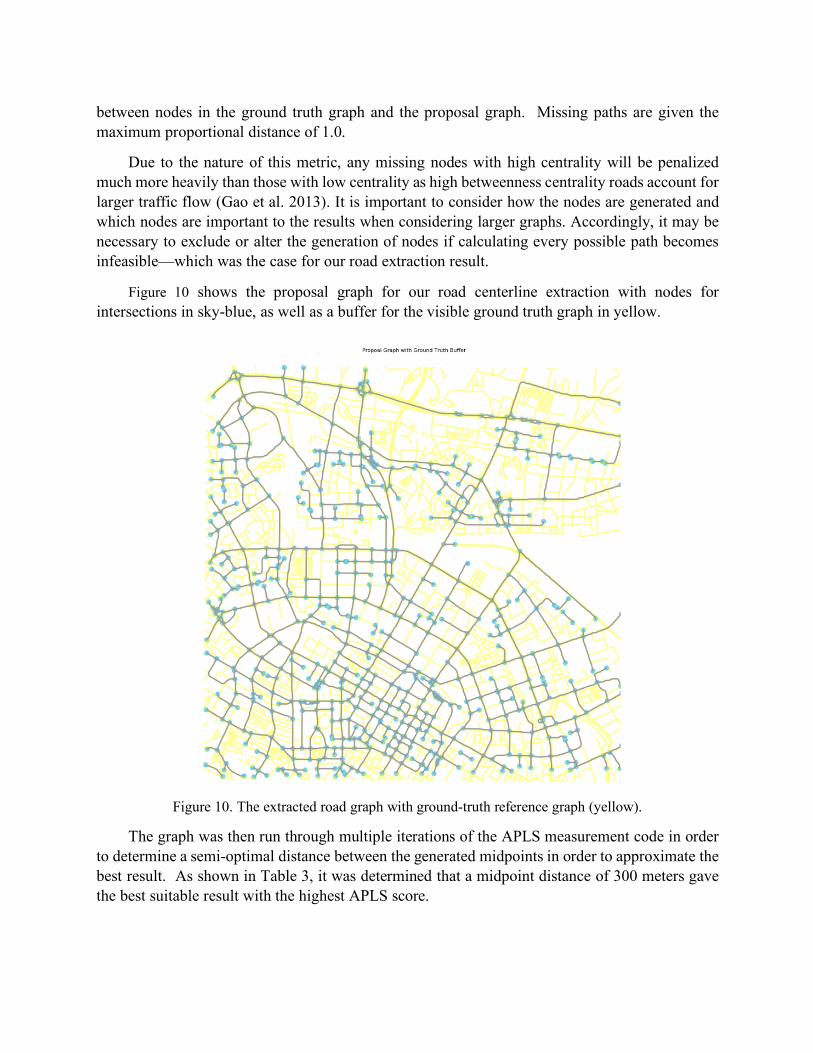
between nodes in the ground truth graph and the proposal graph. Missing paths are given the maximum proportional distance of 1.0.

Due to the nature of this metric, any missing nodes with high centrality will be penalized much more heavily than those with low centrality as high betweenness centrality roads account for larger traffic flow (Gao et al. 2013). It is important to consider how the nodes are generated and which nodes are important to the results when considering larger graphs. Accordingly, it may be necessary to exclude or alter the generation of nodes if calculating every possible path becomes infeasible—which was the case for our road extraction result.

Figure 10 shows the proposal graph for our road centerline extraction with nodes for intersections in sky-blue, as well as a buffer for the visible ground truth graph in yellow.

Figure 10. The extracted road graph with ground-truth reference graph (yellow).

The graph was then run through multiple iterations of the APLS measurement code in order to determine a semi-optimal distance between the generated midpoints in order to approximate the best result. As shown in Table 3, it was determined that a midpoint distance of 300 meters gave the best suitable result with the highest APLS score.

Table 3: Connectivity evaluation results with different distance settings using our proposed approach.

Distance between Midpoints (in meters)

Ground truth nodes snapped to proposal graph

Proposal nodes snapped onto ground truth graph

Total score

100 0.03231549167 0.2753124851 0.05784167 150 0.03251687195 0.2712293888 0.05807170 200 0.03378795578 0.2879258804 0.06047875 250 0.0345725053 0.2801397176 0.06154913 300 0.03618914215 0.2814585314 0.06413233 400 0.03455432375 0.2761312377 0.06142241 450 0.03394610475 0.2779877724 0.06050386 500 0.03480865654 0.2715622517 0.06170766 550 0.03443451154 0.2651631034 0.06095350 600 0.03433385035 0.2690768934 0.06089728 700 0.0344705758 0.2590514352 0.06084485 1000 0.02963361071 0.2431845006 0.05282959

A histogram (in Figure 11) of the results was also created for the path differences when comparing the ground truth graph to the proposal graph, as well as when comparing the path differences from the proposal graph to the ground truth graph. The connectivity results were not good given the aforementioned low coverage completeness of the extracted road networks.

Figure 11. A histogram showing the path differences from proposal (our approach) to ground truth road network.

The same process was repeated to calculate the APLS metric for the baseline approach. Also, a distance of 300 meters between midpoints gave the best result for the total score (as shown in Table 4). However, the total APLS score for the baseline approach was lower than that of our proposed centerline road extraction approach, concluding that our approach provided slightly better connectivity in its resulting road network.

Table 4: Connectivity evaluation results with different distances settings using the baseline approach.

Distance between Midpoints (in meters)

Ground truth nodes snapped onto proposal graph

Proposal nodes snapped onto ground truth graph

Total score

250 0.03069289558 0.2867498315 0.05545052 300 0.03206354837 0.2892501382 0.05772792 328 0.03151483406 0.2834187264 0.05672240 350 0.03110235526 0.2937080329 0.05624827 400 0.03144400797 0.2841326909 0.05662186 450 0.0309466863 0.28561796 0.05584280 500 0.03135845985 0.2761479113 0.05632126 1000 0.02949659611 0.2424995997 0.05259568 2000 0.02970992589 0.2389636115 0.05284920

5 Conclusion and future work

In this chapter, we present a data-driven approach to extracting road centerline geometry information using large-scale GPS trajectory data. The introduced road extraction framework utilizes trajectory compression algorithm (DP), an anisotropic density-based trajectory clustering algorithm (ADCN), and a kernel density estimation and vectorization approach. Compared with remote sensing-based approach, the ride-hailing service GPS trajectory data has a higher spatiotemporal resolution but a smaller geographical coverage. A case study using the DiDi open trajectory dataset in Chengdu, China demonstrates the effectiveness of our proposed approach for extracting road networks. It performed well with regards to the correctness of extracted road networks. However, the connectivity quality is bad due to the large incomplete coverage of the tributary roads. Future work needs to further improve the completeness. In addition, road network includes not only geometry information but also attributes (e.g., number of lanes, one-way restriction, speed limit). Such information may also be extracted from large-scale trajectory datasets with additional attributes (e.g., direction, speed), which require more attention in the road data generation pipeline.

Acknowledgment:

We thank the support of the DiDi Chuxing GAIA Open Dataset Initiative. Dr. Song Gao would like to thank the support for this research provided by the University of Wisconsin - Madison Office of the Vice Chancellor for Research and Graduate Education with funding from the Wisconsin Alumni Research Foundation (WARF).

References: 1. Aronov, B., Driemel, A., Kreveld, M. V., Löffler, M., & Staals, F. (2016). Segmentation of

trajectories on nonmonotone criteria. ACM Transactions on Algorithms (TALG), 12(2), 26.

2. Biagioni, J., & Eriksson, J. (2012, November). Map inference in the face of noise and disparity. In Proceedings of the 20th International Conference on Advances in Geographic Information Systems (pp. 79-88). ACM.

3. Cadez, I., Gaffney, S., & Smyth, P. (2000, March). A general probabilistic framework for clustering individuals. In Proc. of ACM SIGKDD (Vol. 2000).

4. Cao, L., & Krumm, J. (2009, November). From GPS traces to a routable road map. In Proceedings of the 17th ACM SIGSPATIAL international conference on advances in geographic information systems (pp. 3-12). ACM.

5. Davies, J. J., Beresford, A. R., & Hopper, A. (2006). Scalable, distributed, real-time map generation. IEEE Pervasive Computing, 5(4), 47-54.

6. Dijkstra, E. W. (1959). A note on two problems in connexion with graphs. Numerische Mathematik, 1(1), 269-271.

7. Douglas, D. H., & Peucker, T. K. (1973). Algorithms for the reduction of the number of points required to represent a digitized line or its caricature. Cartographica: the International Journal for Geographic Information and Geovisualization, 10(2), 112-122.

8. Ester, M., Kriegel, H. P., Sander, J., & Xu, X. (1996, August). A density-based algorithm for discovering clusters in large spatial databases with noise. In KDD (Vol. 96, No. 34, pp. 226-231).

9. Edelkamp, S., & Schrödl, S. (2003). Route planning and map inference with global positioning traces. In Computer science in perspective (pp. 128-151). Springer, Berlin, Heidelberg.

10. Gaffney, S., & Smyth, P. (1999, August). Trajectory clustering with mixtures of regression models. In KDD (Vol. 99, pp. 63-72).

11. Gao, S., Janowicz, K., Montello, D. R., Hu, Y., Yang, J. A., McKenzie, G., Ju, Y., Gong, L., Adams, B., & Yan, B. (2017). A data-synthesis-driven method for detecting and extracting vague cognitive regions. International Journal of Geographical Information Science, 31(6), 1245-1271.

12. Goodchild, M. F. (2007). Citizens as sensors: web 2.0 and the volunteering of geographic information. GeoFocus. Revista Internacional de Ciencia y Tecnología de la Información Geográfica, (7), 8-10.

13. Hancke, G. P., & Hancke Jr, G. P. (2013). The role of advanced sensing in smart cities. Sensors, 13(1), 393-425.

14. Hu, Y., Gao, S., Janowicz, K., Yu, B., Li, W., & Prasad, S. (2015). Extracting and understanding urban areas of interest using geotagged photos. Computers, Environment and Urban Systems, 54, 240-254.

15. Jiang Y, Li X, Li X J, et al. Geometrical characteristics extraction and accuracy analysis of road network based on vehicle trajectory data[J]. Journal of Geo-information Science, 2012, 14(2): 165-170.

16. Kolatch, E. (2001). Clustering algorithms for spatial databases: A survey. 1-22.

17. Kuntzsch, C., Sester, M., & Brenner, C. (2016). Generative models for road network reconstruction. International Journal of Geographical Information Science, 30(5), 1012-1039.

18. Lang, T. (1969). Rules for the robot draughtsmen. The Geographical Magazine, 42(1), 50-51. 19. Lee, J. G., Han, J., & Whang, K. Y. (2007, June). Trajectory clustering: a partition-and-group

framework. In Proceedings of the 2007 ACM SIGMOD international conference on Management of data (pp. 593-604). ACM.

20. Li, J., Qin, Q., Xie, C., & Zhao, Y. (2012). Integrated use of spatial and semantic relationships for extracting road networks from floating car data. International Journal of Applied Earth Observation and Geoinformation, 19, 238-247.

21. Li, Z., Lee, J. G., Li, X., & Han, J. (2010, April). Incremental clustering for trajectories. In International Conference on Database Systems for Advanced Applications (pp. 32-46). Springer, Berlin, Heidelberg.

22. Liu, Y., Wang, F., Xiao, Y., & Gao, S. (2012). Urban land uses and traffic ‘source-sink areas’: Evidence from GPS-enabled taxi data in Shanghai. Landscape and Urban Planning, 106(1), 73-87.

23. McMaster, R. B. (1989). The integration of simplification and smoothing algorithms in line generalization. Cartographica: The International Journal for Geographic Information and Geovisualization, 26(1), 101-121.

24. Mai, G., Janowicz, K., Hu, Y., & Gao, S. (2018). ADCN: An anisotropic density-based clustering algorithm for discovering spatial point patterns with noise. Transactions in GIS, 22(1), 348-369.

25. Opheim, H. (1982). ‘Fast data reduction of a digitized curve’, GeoProcessing, 2, 33–40. 26. Reumann, K. & Witkam, A. P. M. (1974). Optimizing Curve Segmantation in Computer Graphics.

International Comp. Sympo. 1973. Amsterdam, 467-472.

27. Shaw, S. L. (2010). Geographic information systems for transportation: from a static past to a dynamic future. Annals of GIS, 16(3), 129-140.

28. Shi, W., & Cheung, C. (2006). Performance evaluation of line simplification algorithms for vector generalization. The Cartographic Journal, 43(1), 27-44.

29. Shi, W., Shen, S., & Liu, Y. (2009, October). Automatic generation of road network map from massive GPS, vehicle trajectories. In 2009 12th International IEEE Conference on Intelligent Transportation Systems (pp. 1-6). IEEE.

30. Silverman, B. W. (1986). Density Estimation for Statistics and Data Analysis. London: Chapman & Hall.

31. Stanojevic, R., Abbar, S., Thirumuruganathan, S., Chawla, S., Filali, F., & Aleimat, A. (2018, May). Robust road map inference through network alignment of trajectories. In Proceedings of the 2018 SIAM International Conference on Data Mining (pp. 135-143). Society for Industrial and Applied Mathematics.

32. Tao, C. V. (2000). Mobile mapping technology for road network data acquisition. Journal of Geospatial Engineering, 2(2), 1-14.

33. Tang, L., Ren, C., Liu, Z., & Li, Q. (2017). A road map refinement method using Delaunay triangulation for big trace data. ISPRS International Journal of Geo-Information, 6(2), 45.

34. Worrall, S., & Nebot, E. (2007, December). Automated process for generating digitised maps through GPS data compression. In Australasian Conference on Robotics and Automation (Vol. 6). Brisbane: ACRA.

35. Wang, S., Wang, Y., & Li, Y. (2015, November). Efficient map reconstruction and augmentation via topological methods. In Proceedings of the 23rd SIGSPATIAL International Conference on Advances in Geographic Information Systems (pp. 1-10).

36. Wang, J., Rui, X., Song, X., Tan, X., Wang, C., & Raghavan, V. (2015). A novel approach for generating routable road maps from vehicle GPS traces. International Journal of Geographical Information Science, 29(1), 69-91.

37. Wiedemann, C., Heipke, C., Mayer, H., & Jamet, O. (1998). Empirical evaluation of automatically extracted road axes. In Empirical evaluation techniques in computer vision (Vol. 12, pp. 172-187). Los Alamitos, CA: IEEE Computer Society Press.

38. Wu, J., Zhu, Y., Ku, T., & Wang, L. (2013). Detecting Road Intersections from Coarse-gained GPS Traces Based on Clustering. JCP, 8(11), 2959-2965.

39. Wang, H., Li, Y., Liu, G., Wen, X., & Qie, X. (2019). Accurate Detection of Road Network Anomaly by Understanding Crowd's Driving Strategies from Human Mobility. ACM Transactions on Spatial Algorithms and Systems (TSAS), 5(2), 11.

40. Wu, C., Ayers, P. D., & Anderson, A. B. (2007). Validating a GIS-based multi-criteria method for potential road identification. Journal of Terramechanics, 44(3), 255-263.

41. Yuan, N. J., Zheng, Y., & Xie, X. (2012). Segmentation of urban areas using road networks. MSR-TR-2012–65, Tech. Rep.

42. Zhao, Y., Liu, J., Chen, R., Li, J., Xie, C., Niu, W., Geng, D., & Qin, Q. (2011, July). A new method of road network updating based on floating car data. In 2011 IEEE International Geoscience and Remote Sensing Symposium (pp. 1878-1881). IEEE.

43. Zheng, Y. (2015). Trajectory data mining: an overview. ACM Transactions on Intelligent Systems and Technology (TIST), 6(3), 29.