AUTOMATIC STRUCTURES OF BOUNDED DEGREE REVISITED · AUTOMATIC STRUCTURES OF BOUNDED DEGREE...
30
The Journal of Symbolic Logic Volume 00, Number 0, XXX 0000 AUTOMATIC STRUCTURES OF BOUNDED DEGREE REVISITED DIETRICH KUSKE AND MARKUS LOHREY Abstract. The first-order theory of a string automatic structure is known to be decid- able, but there are examples of string automatic structures with nonelementary first-order theories. We prove that the first-order theory of a string automatic structure of bounded degree is decidable in doubly exponential space (for injective automatic presentations, this holds even uniformly). This result is shown to be optimal since we also present a string automatic structure of bounded degree whose first-order theory is hard for 2EXPSPACE. We prove similar results also for tree automatic structures. These findings close the gaps left open in [28] by improving both the lower and the upper bounds. §1. Introduction. The idea of an automatic structure goes back to B¨ uchi and Elgot who used finite automata to decide, e.g., Presburger arithmetic [14]. Automaton decidable theories [18] and automatic groups [15] are similar con- cepts. A systematic study was initiated by Khoussainov and Nerode [20] who also coined the name “automatic structure” (we prefer the term “string auto- matic structure” in this paper). In essence, a structure is string automatic if the elements of the universe can be represented as strings from a regular language (an element can be represented by several strings) and every relation of the structure can be recognized by a finite state automaton with several heads that proceed synchronously. String automatic structures received increasing interest over the last years [1, 3, 4, 5, 7, 17, 19, 21, 22, 24, 27, 31]. One of the main motivations for investigating string automatic structures is that their first-order theories can be decided uniformly (i.e., the input is a string automatic presen- tation and a first-order sentence). But even the non-uniform first-order theory is far from efficient since there exist string automatic structures with a nonele- mentary first-order theory. This motivates the search for subclasses of string automatic structures whose first-order theories are elementary. The first such class was identified by the second author in [28] who showed that the first-order theory of every string automatic structure of bounded degree can be decided in triply exponential alternating time with linearly many alternations. A structure 1991 Mathematics Subject Classification. This is not required. Key words and phrases. This is not required. The second author acknowledges support from the DFG-project GELO.These results were obtained when Dietrich Kuske was affiliated with the Institut f¨ ur Informatik, Universit¨ at Leipzig. c 0000, Association for Symbolic Logic 0022-4812/00/0000-0000/$00.00 1
Transcript of AUTOMATIC STRUCTURES OF BOUNDED DEGREE REVISITED · AUTOMATIC STRUCTURES OF BOUNDED DEGREE...

The Journal of Symbolic Logic
Volume 00, Number 0, XXX 0000
AUTOMATIC STRUCTURES OF BOUNDED DEGREE REVISITED
DIETRICH KUSKE AND MARKUS LOHREY
Abstract. The first-order theory of a string automatic structure is known to be decid-
able, but there are examples of string automatic structures with nonelementary first-order
theories. We prove that the first-order theory of a string automatic structure of bounded
degree is decidable in doubly exponential space (for injective automatic presentations, this
holds even uniformly). This result is shown to be optimal since we also present a string
automatic structure of bounded degree whose first-order theory is hard for 2EXPSPACE.
We prove similar results also for tree automatic structures. These findings close the gaps
left open in [28] by improving both the lower and the upper bounds.
§1. Introduction. The idea of an automatic structure goes back to Buchiand Elgot who used finite automata to decide, e.g., Presburger arithmetic [14].Automaton decidable theories [18] and automatic groups [15] are similar con-cepts. A systematic study was initiated by Khoussainov and Nerode [20] whoalso coined the name “automatic structure” (we prefer the term “string auto-matic structure” in this paper). In essence, a structure is string automatic if theelements of the universe can be represented as strings from a regular language(an element can be represented by several strings) and every relation of thestructure can be recognized by a finite state automaton with several heads thatproceed synchronously. String automatic structures received increasing interestover the last years [1, 3, 4, 5, 7, 17, 19, 21, 22, 24, 27, 31]. One of the mainmotivations for investigating string automatic structures is that their first-ordertheories can be decided uniformly (i.e., the input is a string automatic presen-tation and a first-order sentence). But even the non-uniform first-order theoryis far from efficient since there exist string automatic structures with a nonele-mentary first-order theory. This motivates the search for subclasses of stringautomatic structures whose first-order theories are elementary. The first suchclass was identified by the second author in [28] who showed that the first-ordertheory of every string automatic structure of bounded degree can be decided intriply exponential alternating time with linearly many alternations. A structure
1991 Mathematics Subject Classification. This is not required.Key words and phrases. This is not required.The second author acknowledges support from the DFG-project GELO.These results were
obtained when Dietrich Kuske was affiliated with the Institut fur Informatik, UniversitatLeipzig.
c© 0000, Association for Symbolic Logic
0022-4812/00/0000-0000/$00.00
1

2 DIETRICH KUSKE AND MARKUS LOHREY
has bounded degree, if in its Gaifman graph, the number of neighbors of a node isbounded by some fixed constant. The paper [28] also presents a specific exampleof a string automatic structure of bounded degree, where the first-order theoryis hard for doubly exponential alternating time with linearly many alternations.Hence, an exponential gap between the upper and lower bound remained. Anupper bound of 4-fold exponential alternating time with linearly many alterna-tions was shown for tree automatic structures (which are defined analogously toautomatic structures using tree automata) of bounded degree. Our paper [25]proves a triply exponential space bound for the first-order theory of an injectiveω-string automatic structure (that is defined via Buchi-automata) of boundeddegree. Here, injectivity means that every element of the structure is representedby a unique ω-string from the underlying regular language. By [17], the classof injective ω-string automatic structures is a strict subclass of the class of allω-string automatic structures, whereas for string and tree automatic structuresinjectivity is not a restriction [9, 20, 35].
In this paper, we achieve three goals:
• We close the complexity gaps from [28] for string/tree automatic structuresof bounded degree.
• We investigate, for the first time, the complexity of the uniform first-ordertheory (where the automatic presentation is part of the input) of string/treeautomatic structures of bounded degree.
• We refine our complexity analysis using the growth function of a structure.This function measures the size of a sphere in the Gaifman graph dependingon the radius of the sphere. The growth function of a structure of boundeddegree can be at most exponential.
Our main results are the following:
• The uniform first-order theory for injective string automatic presentationsof bounded degree is 2EXPSPACE-complete. The lower bound already holdsin the non-uniform setting, i.e., there exists a string automatic structure ofbounded degree with a 2EXPSPACE-complete first-order theory.
• For every string automatic structure of bounded degree, where the growthfunction is polynomially bounded, the first-order theory is in EXPSPACE,and there exists an example with an EXPSPACE-complete first-order theory.
• The uniform first-order theory for injective tree automatic presentationsof bounded degree belongs to 4EXPTIME. For every fixed tree automaticstructure of bounded degree, the first-order theory belongs to 3EXPTIME,and to 2EXPTIME if the growth function is polynomial. Our bounds forthe non-uniform problem are sharp, i.e., there are tree automatic structuresof bounded degree (and polynomial growth) with a 3EXPTIME-complete(2EXPTIME-complete, resp.) first-order theory.
For the uniform first-order theory for injective tree automatic presentations ofbounded degree, the precise complexity remains open (it is in 4EXPTIME and3EXPTIME-hard). If the input presentations are not necessarily injective, theupper bounds for the uniform theories are one exponent higher: 3EXPSPACE inthe string case and 5EXPTIME in the tree case. We conclude this paper withsome results on the complexity of first-order fragments with fixed quantifier

AUTOMATIC STRUCTURES OF BOUNDED DEGREE REVISITED 3
alternation depth one or two on string/tree automatic structures of boundeddegree.
Further related work. In [12] the blow-up in formula size inherent in Gaifman’slocality theorem has been investigated. That work reveals that in the worst casea non-elementary blow-up is unavoidable already on locally finite structures (infact, forests). In the same paper it is also remarked that on (not necessarilyautomatic) structures of bounded degree every first-order formula is equivalentto a Boolean combination of basic local sentences of at most 4-fold exponentialtotal size. In some sense, our results refine this result for the case of automaticstructures of bounded degree.
In [2], Barany considers p-automatic structures, which are string automaticstructures having an automatic presentation with a domain language of polyno-mial growth (i.e., the number of words of length at most n grows polynomiallywith n). For each of these structures, the first-order theory belongs to PSPACE.A p-automatic structure of bounded degree must have polynomial growth in thesense used in this paper. On the other hand, p-automatic structures are notrequired to be of bounded degree. Moreover, our example of an automatic struc-ture of bounded degree with polynomial growth and an EXPSPACE-completefirst-order theory is not p-automatic (since PSPACE ( EXPSPACE by the spacehierarchy theorem). Hence, the class of p-automatic structures and the class ofbounded degree automatic structures of polynomial growth are incomparable.
§2. Preliminaries. Let Γ be a finite alphabet and w ∈ Γ∗ be a finite wordover Γ. The length of w is denoted by |w|. Let Γn = w ∈ Γ∗ | n = |w|.
Let us define exp(0, x) = x and exp(n + 1, x) = 2exp(n,x) for x ∈ N. Weassume that the reader has some basic knowledge in complexity theory, seee.g. [30]. By Savitch’s theorem, NSPACE(s(n)) ⊆ DSPACE(s(n)2) if s(n) ≥log(n). Hence, we can just write SPACE(s(n)O(1)) for either NSPACE(s(n)O(1)) orDSPACE(s(n)O(1)). For k ≥ 1, we denote with kEXPSPACE (resp. kEXPTIME)the class of all problems that can be accepted in space (resp. time) exp(k, nO(1))on a deterministic Turing machine. For 1EXPSPACE we write just EXPSPACE
and 0EXPSPACE stands for PSPACE. A computational problem is called elemen-tary if it belongs to kEXPTIME for some k ∈ N.
2.1. Tree and string automata. For our purpose it suffices to consideronly tree automata on binary trees. Let Γ be a finite alphabet. A finite binarytree over Γ is a mapping t : dom(t) → Γ, where dom(t) ⊆ 0, 1∗ is finite,nonempty, and satisfies the following closure condition for all w ∈ 0, 1∗: ifw0, w1 ∩ dom(t) 6= ∅, then also w,w0 ∈ dom(t). With TΓ we denote the setof all finite binary trees over Γ. A (top-down) tree automaton over Γ is a tupleA = (Q,∆, q0), where Q is the finite set of states, q0 ∈ Q is the initial state, and
∆ ⊆ (Q× Γ ×Q×Q) ∪ (Q× Γ ×Q) ∪ (Q× Γ) (1)
is the non-empty transition relation. A successful run of A on a tree t is a map-ping ρ : dom(t) → Q such that (i) ρ(ε) = q0 and (ii) for every w ∈ dom(t) withchildren w0, . . . , wi (thus −1 ≤ i ≤ 1) we have (ρ(w), t(w), ρ(w0), . . . , ρ(wi)) ∈∆. With L(A) we denote the set of all finite binary trees t such that there exists

4 DIETRICH KUSKE AND MARKUS LOHREY
a successful run of A on t. A set L ⊆ TΓ is called regular if there exists a finitetree automaton A with L = L(A).
A tree t with dom(t) ⊆ 0∗ and n = |dom(t)| can be identified with thenonempty string t(ε)t(0)t(00) . . . t(0n−1). In the same spirit, a finite string au-tomaton can be defined as a tree automaton, where the transition relation ∆ in(1) satisfies ∆ ⊆ (Q× Γ ×Q) ∪ (Q× Γ).
We will need the following well known facts on string/tree automata: Empti-ness (resp. inclusion) of the languages of string automata can be decided innondeterministic logarithmic space (resp. polynomial space), whereas emptiness(resp. inclusion) of the languages of tree automata can be decided in polynomialtime (resp. exponential time), see e.g. [10]. In all four cases completeness holds.
2.2. Structures and first-order logic. A signature is a finite set S of re-lational symbols, where every symbol r ∈ S has some fixed arity mr. Thenotion of an S-structure (or model) is defined as usual in logic. Note that weonly consider relational structures. Sometimes, we will also use constants, butin our context, a constant c can be always replaced by the unary relation c.Let us fix an S-structure A = (A, (rA)r∈S), where rA ⊆ Amr . To simplifynotation, we will write a ∈ A for a ∈ A. For B ⊆ A we define the restric-tion AB = (B, (rA ∩ Bmr )r∈S). Given further constants a1, . . . , an ∈ A, wewrite (A, a1, . . . , ak) for the structure (A, (rA)r∈S , a1, . . . , ak). In the rest of thepaper, we will always identify a symbol r ∈ S with its interpretation rA.
A congruence on the structure A = (A, (r)r∈S) is an equivalence relation ≡on A such that for every r ∈ S and all a1, b1, . . . , amr
, bmr∈ A we have: If
(a1, . . . , amr) ∈ r and a1 ≡ b1, . . . , amr
≡ bmr, then also (b1, . . . , bmr
) ∈ r. Asusual, the equivalence class of a ∈ A w.r.t. ≡ is denoted by [a]≡ or just [a] andA/≡ denotes the set of all equivalence classes. We define the quotient structureA/≡ = (A/≡, (r/≡)r∈S), where r/≡ = ([a1], . . . , [amr
]) | (a1, . . . , amr) ∈ r.
The Gaifman graph G(A) of the S-structure A is the following symmetricgraph:
G(A) = (A, (a, b) ∈ A×A |∨
r∈S∃(a1, . . . , amr
) ∈ r ∃j, k : aj = a, ak = b)
Thus, the set of nodes is the universe of A and there is an edge between twoelements, if and only if they are contained in some tuple belonging to one of therelations of A. With dA(a, b), where a, b ∈ A, we denote the distance between aand b in G(A), i.e., it is the length of a shortest path connecting a and b in G(A).For a ∈ A and d ≥ 0 we denote with SA(d, a) = b ∈ A | dA(a, b) ≤ d the d-sphere around a. If A is clear from the context, then we will omit the subscript A.We say that the structure A is locally finite if its Gaifman graph G(A) is locallyfinite (i.e., every node has finitely many neighbors). Similarly, the structure Ahas bounded degree, if G(A) has bounded degree, i.e., there exists a constant δsuch that every a ∈ A is adjacent to at most δ many other nodes in G(A);the minimal such δ is called the degree of A. For a structure A of boundeddegree we can define its growth function as the mapping gA : N → N withgA(n) = max|SA(n, a)| | a ∈ A. Note that if the function gA is not boundedthen gA(n) ≥ n for all n ≥ 1. For us, it is more convenient to not have a boundedfunction describing the growth. Therefore, we define the normalized growth
AUTOMATIC STRUCTURES OF BOUNDED DEGREE REVISITED 5
function g′A by g′A(n) = maxn, gA(n). Note that gA and g′A are different onlyin the pathological case that all connected components of A contain at mostm elements (for some fixed m). Clearly, g′A(n) can grow at most exponentially(since A is assumed to have bounded degree). We say that A has exponentialgrowth if g′A(n) ∈ 2Ω(n); if g′A(n) ∈ nO(1), then A has polynomial growth.
To define logical formulas, we fix a countably infinite set V of variables, whichevaluate to elements of structures. Formulas over the signature S (or formulas ifthe signature is clear from the context) are constructed from the atomic formulasx = y and r(x1, . . . , xmr
), where r ∈ S and x, y, x1, . . . , xmr∈ V , using the
Boolean connectives ∨ and ¬ and existential quantification over variables from V .The Boolean connective ∧ and universal quantification can be derived from theseoperators in the usual way. The quantifier depth of a formula ϕ is the maximalnesting depth of quantifiers in ϕ. The notion of a free variable is defined asusual. A formula without free variables is called closed. If ϕ(x1, . . . , xm) is aformula with free variables among x1, . . . , xm and a1, . . . , am ∈ A, then A |=ϕ(a1, . . . , am) means that ϕ evaluates to true in A when the free variable xi
evaluates to ai. The first-order theory of A, denoted by FOTh(A), is the set ofall closed formulas ϕ such that A |= ϕ. For n ≥ 0, Σn-formulas and Πn-formulasare inductively defined as follows:
• A quantifier-free first-order formula is a Σ0-formula as well as a Π0-formula.• If ϕ(x1, . . . , xn, y) is a Σn-formula, then ∀x1 · · · ∀xn : ϕ(x1, . . . , xn, y) is a
Πn+1-formula.• If ϕ(x1, . . . , xn, y) is a Πn-formula, then ∃x1 · · · ∃xn : ϕ(x1, . . . , xn, y) is a
Σn+1-formula.
The Σn-theory Σn-FOTh(A) of a structure A is the set of all Σn-formulas inFOTh(A); the Πn-theory is defined analogously.
2.3. Structures from automata. This section recalls string automatic andtree automatic structures and basic results about them. Details can be found inthe surveys [31, 3].
2.3.1. Tree and string automatic structures. String automatic structures wereintroduced in [18], their systematic study was later initiated by [20]. Tree auto-matic structures were introduced in [6], they generalize string automatic struc-tures. Here, we will first introduce tree automatic structures. String automaticstructures can be considered as a special case of tree automatic structures.
Let Γ be a finite alphabet and let $ 6∈ Γ be an additional padding symbol. Lett1, . . . , tm ∈ TΓ. We define the convolution t = t1 ⊗ · · · ⊗ tm, which is a finitebinary tree over the alphabet (Γ ∪ $)m, as follows: dom(t) =
⋃mi=1 dom(ti)
and for all w ∈ ⋃mi=1 dom(ti) we define t(w) = (a1, . . . , am), where ai = ti(w) if
w ∈ dom(ti) and ai = $ otherwise. In Fig. 1, the third tree is the convolution ofthe first two trees.
An m-dimensional (synchronous) tree automaton over Γ is just a tree automa-ton A over the alphabet (Γ∪$)m such that L(A) ⊆ t1⊗· · ·⊗ tn | t1, . . . , tm ∈TΓ. Such an automaton defines an m-ary relation
R(A) = (t1, . . . , tm) | t1 ⊗ · · · ⊗ tm ∈ L(A) .
A tree automatic presentation is a tuple P = (Γ, A0, A=, (Ar)r∈S), where:

6 DIETRICH KUSKE AND MARKUS LOHREY
a
b b
a a
a
a
b b
a
(a, a)
(b, $) (b, a)
(a, $) (a, $) ($, b) ($, b)
($, a)
Figure 1. The convolution of two trees
• Γ is a finite alphabet.• S is a signature (the signature of P ), as before mr is the arity of the symbolr ∈ S.
• A0 is a tree automaton over the alphabet Γ.• For every r ∈ S, Ar is an mr-dimensional tree automaton over the alphabet
Γ ∪ $ such that R(Ar) ⊆ L(A0)mr .
• A= is a 2-dimensional tree automaton over the alphabet Γ ∪ $ such thatR(A=) ⊆ L(A0) × L(A0) and R(A=) is a congruence on the structure(L(A0), (R(Ar))r∈S).
This presentation P is called injective if R(A=) is the identity relation on L(A0).In this case, we can omit the automaton A= and identify P with the tuple(Γ, A0, (Ar)r∈S). The structure presented by P is the quotient
A(P ) = (L(A0), (R(Ar))r∈S)/R(A=) .
A structure A is called tree automatic if there exists a tree automatic presen-tation P such that A ≃ A(P ). We will write [u] for the element [u]R(A=)
(u ∈ L(A0)) of the structure A(P ). We say that the presentation P has boundeddegree if the structure A(P ) has bounded degree.
A string automatic presentation is a tree automatic presentation, where alltree automata are in fact string automata (as explained in Section 2.1), and astructure A is called string automatic if there exists a string automatic presen-tation P such that A ≃ A(P ). Typical examples of string automatic structuresare (N,+) (Presburger’s arithmetic), (Q,≤), and all ordinals below ωω [13, 20].An example of a tree automatic structure, which is not string automatic is (N, ·)(the natural numbers with multiplication) [6], or the ordinal ωω [13]. Examplesof string automatic structures of bounded degree are transition graphs of Turingmachines and Cayley-graphs of automatic groups [15] (or even right-cancellativemonoids [33]).
Remark 2.1. Usually a tree automatic presentation for an S-structure A =(A, (r)r∈S ) is defined as a tuple (Γ, L, h) such that
• Γ is a finite alphabet,• L ⊆ TΓ is a regular set of trees,• h : L→ A is a surjective function,• the relation (u, v) ∈ L × L | h(u) = h(v) can be recognized by a 2-
dimensional tree automaton, and

AUTOMATIC STRUCTURES OF BOUNDED DEGREE REVISITED 7
• for all r ∈ S, the relation (u1, . . . , umr) ∈ Lmr | (h(u1), . . . , h(umr
)) ∈ rcan be recognized by an mr-dimensional tree automaton.
Since for our considerations, tree automatic presentations are part of the inputfor algorithms, we prefer our definition, where a tree automatic presentation is afinite object (a tuple of finite tree automata), whereas in the standard definition,the presentation also contains the presentation map h.
Let SA be the class of all string automatic presentations and let TA be theclass of all tree automatic presentations. Moreover, for X ∈ SA,TA let
Xb = P ∈ X | A(P ) has bounded degreeiX = P ∈ X | P is injective
iXb = Xb ∩ iX
2.3.2. The model checking problem. For the above classes of tree automaticpresentations, we will be interested in the following decision problems.
Definition 2.2. Let C be a class of tree automatic presentations.
• The first-order model checking problem FOMC(C) for C denotes the set ofall pairs (P, ϕ), where P ∈ C and ϕ ∈ FOTh(A(P )).
• For n ≥ 1, the Σn-model checking problem Σn-FOMC(C) for C denotes theset of all pairs (P, ϕ), where P ∈ C and ϕ ∈ Σn-FOTh(A(P )).
If C = P is a singleton, then the model checking problem FOMC(C) for C
can be identified with the first-order theory of the structure A(P ). An algorithmdeciding the model checking problem for a nontrivial class C decides the first-order theories of each element of C uniformly.
The following two results are the main motivations for investigating tree au-tomatic structures.
Proposition 2.3 ([6, 20]). There is an algorithm that computes from a treeautomatic presentation P = (Γ, A0, A=, (Ar)r∈S) and a formula ϕ(x1, . . . , xm)an m-dimensional tree automaton A over Γ with R(A) = (u1, . . . , um) ∈L(A0)
m | A(P ) |= ϕ([u1], . . . , [um]).The automaton is constructed by induction on the structure of the formula ϕ:
disjunction corresponds to the disjoint union of automata, existential quantifi-cation to projection, and negation to complementation. The following result isa direct consequence.
Theorem 2.4 ([6, 20]). The model checking problem FOMC(TA) for all treeautomatic presentations is decidable. In particular, for every tree automaticstructure A the first-order theory FOTh(A) is decidable.
Remark 2.5. Strictly speaking, [6, 20] devise algorithms that, given a treeautomatic presentation and a closed formula, decide whether the formula holdsin the presented structure. But a priori, it is not clear whether it is decid-able, whether a given tuple (Γ, A0, A=, (Ar)r∈S) is a tree automatic presentation.Lemma 2.12 below shows that TA is indeed decidable, which then completes theproof of Theorem 2.4.

8 DIETRICH KUSKE AND MARKUS LOHREY
Theorem 2.4 holds even if we add quantifiers for “there are infinitely many xsuch that ϕ(x)” [6, 7] and “the number of elements satisfying ϕ(x) is divisibleby k” (for k ∈ N) [23]1. This implies in particular that it is decidable whethera tree automatic presentation describes a locally finite structure. But the decid-ability of the first-order theory is far from efficient, since there are even stringautomatic structures with a nonelementary first-order theory [7]. For instancethe structure (0, 1∗, s0, s1,), where si = (w,wi) | w ∈ 0, 1∗ for i ∈ 0, 1and is the prefix order on finite words, has a nonelementary first-order theory,see e.g. [11, Example 8.3]. In fact, even locally finite examples exist:
Proposition 2.6. There exists a locally finite string automatic structure witha nonelementary first-order theory.
Proof. The theory of all finite binary labeled linear orders is nonelemen-tary [29]. Since this theory can be reduced to the first-order theory of the struc-ture consisting of the disjoint union of all finite binary labeled linear orders, thelatter structure has a nonelementary first-order theory too. But this structureis automatic: The universe is the set L = u⊗ v | u ∈ 0, 1+, v ∈ 0∗, |v| < |u|.In addition, we have a partial order (u ⊗ v, u ⊗ v′) ∈ L × L | |v| ≤ |v′|that encodes the union of all the linear order relations, and a unary relationu⊗ v ∈ L | position |v| in u carries 1 that encodes the labeling. ⊣
The following two results refine Theorem 2.4:
Theorem 2.7 ([26]). The following holds for all n ≥ 0:
(1) The Σn+1-model checking problem Σn+1-FOMC(SA) for all string automaticpresentations is in nEXPSPACE.
(2) There is a fixed string automatic structure with an nEXPSPACE-completeΣn+1-theory.
(3) There is a closed formula ϕn ∈ Σn+1 for which P ∈ SA | A(P ) |= ϕn isnEXPSPACE-complete.
Remark 2.8. For n = 0 and n = 1, the above statement (2) can be foundin [3]. Regarding (1) and (3), an exponentially better bound holds for automaticpresentations that consist of deterministic automata, only: for n ≤ 1, this canbe found in [3], the general case can be shown using the methods from [26].
Theorem 2.9. For all n ≥ 1, the Σn-model checking problem Σn-FOMC(TA)for all tree automatic presentations is in nEXPTIME.
In [26] only Theorem 2.7 is shown. But the proof for Theorem 2.9 is almost thesame as for the first statement of Theorem 2.7. The only difference comes fromthe fact that emptiness for string automata is NL-complete, whereas emptinessfor tree automata is P-complete.
2.3.3. First complexity results: the classes TA etc and boundedness. This pa-per is concerned with the uniform and non-uniform complexity of the first-ordertheory of (some subclass of) tree automatic structures of bounded degree. Thus,
1[23] only provides the proofs for string automatic structures. These proofs are easily ex-tended to tree automatic structures once the presentation is injective. But every tree automaticpresentation can be transformed into an equivalent injective one [9, 35].

AUTOMATIC STRUCTURES OF BOUNDED DEGREE REVISITED 9
we will consider algorithms that take as input tree automatic presentations (to-gether with closed formulas). For complexity considerations, we have to definethe size |P | of a tree automatic presentation P = (Γ, A0, A=, (Ar)r∈S). First, letus define the size |A| of an m-dimensional tree automaton A = (Q,∆, q0) over Γ.A transition tuple from ∆ (see (1)) can be stored with at most 3 log(|Q|) +m log(|Γ|) many bits. Hence, up to constant factors, ∆ can be stored in space|∆| · (log(|Q|) +m log(|Γ|)). We can assume that every state is the first compo-nent of some transition tuple, i.e., |Q| ≤ |∆|. Furthermore, the size of the basicalphabet Γ can be bounded by |∆| as well, but the dimension m is independentfrom the size of ∆. Since our complexity measures will be up to polynomial timereductions, it therefore makes sense to define the size of the tree automaton Ato be |A| = |∆| · m. We assume ∆ to be nonempty, hence |A| ≥ 1. The sizeof the presentation P = (Γ, A0, A=, (Ar)r∈S) is |P | = |A0| + |A=| +
∑
r∈S |Ar|.Note that |S| ≤ |P | and m ≤ |P |, when m is the maximal arity in S.
It will be convenient to work with injective string (resp. tree) automatic pre-sentations. The following lemma says that this is no restriction, at least if we donot consider complexity aspects.
Lemma 2.10 ([20, Corollary 4.3] and [35]). From a given P ∈ TA (resp. P ∈SA) one can compute in time 2O(|P |) a presentation P ′ ∈ iTA (resp. P ′ ∈ iSA)with A(P ) ≃ A(P ′).
Remark 2.11. For string automatic presentations, the statement of Lemma 2.10was shown in [20]. Although the exponential time bound on the constructionof P ′ ∈ iSA is not stated explicitly in [20], it can be easily extracted from theconstruction. In [9, Corollary 4.2], it is stated that for every P ∈ TA there existsP ′ ∈ iTA with A(P ) ≃ A(P ′). Although the construction of P ′ is effective,the complexity is difficult to extract from [9]. An exponential construction ofP ′ ∈ iTA was presented in [35].
The following lemma shows that the classes of all tree and string automaticpresentations are decidable and gives complexity bounds. While these two resultsare not surprising, it is not clear how to determine whether A(P ) has boundeddegree – this will be solved by Proposition 2.14 below.
Lemma 2.12. The class TA is EXPTIME-complete and the class SA is PSPACE-complete.
Proof. We start with a proof of the first statement. Suppose we are givena tuple of tree automata A0, A=, (Ar)r∈S over an alphabet Γ. In a first step,we check in polynomial time, whether A= is a 2-dimensional tree automatonover Γ and that every Ar (r ∈ S) is an mr-dimensional tree automaton over Γaccording to Section 2.3.1. We proceed as follows for every r ∈ S (for A= thesame algorithm works):
First, we check that no tree from L(Ar) contains the label ($, . . . , $). To thisaim, replace in all transitions of Ar the letters from (Γ∪$)mr \ ($, . . . , $) by⊤ and the letter ($, . . . , $) by ⊥ and check whether the language of the resultingautomaton is contained in T⊤ (the set of all ⊤-labeled binary trees). Since theset T⊤ can be accepted by a fixed automaton, this inclusion can be decidedin polynomial time. Hence, we can assume that no tree from L(Ar) contains

10 DIETRICH KUSKE AND MARKUS LOHREY
the label ($, . . . , $). Next, let H ⊆ T⊤,$ denote the set of those trees t whose⊤-labeled nodes form an initial segment of t. Again this set can be accepted bya fixed automaton. For all 1 ≤ i ≤ mr we construct (in polynomial time) anautomaton Ar,i as follows: First we project Ar onto its ith component. Then, wereplace in every transition of the resulting automaton all occurrences of symbolsfrom Γ by ⊤. It remains to check that L(Ar,i) ⊆ H for all 1 ≤ i ≤ mr, whichcan be done in polynomial time.
For the rest of the proof, let us assume that A= is a 2-dimensional tree automa-ton over Γ and that everyAr (r ∈ S) is anmr-dimensional tree automaton over Γ.This implies that the tuple P = (Γ, B,A0, A=, (Ar)r∈S), where L(B) = TΓ, isan injective tree automatic presentation. Here, A0 defines a unary relation onthe domain TΓ, and A= defines a binary relation. Then, (Γ, A0, A=, (Ar)r∈S)is a tree automatic presentation if and only if the following closed first-orderformulas are true in S(P ′) for all r ∈ S:
∀x, y : (x, y) ∈ R(A=) → x, y ∈ L(A0)
∀x ∈ L(A0) : (x, x) ∈ R(A=)
∀x, y ∈ L(A0) : (x, y) ∈ R(A=) → (y, x) ∈ R(A=)
∀x, y, z ∈ L(A0) : ((x, y) ∈ R(A=) ∧ (y, z) ∈ R(A=)) → (x, z) ∈ R(A=)
∀x1, . . . , xmr: (x1, . . . , xmr
) ∈ R(Ar) → x1, . . . , xmr∈ L(A0)
∀(x1, y1), . . . , (xmr, ymr
) ∈ R(A=)
(
(x1, . . . , xmr) ∈ R(Ar) →
(y1, . . . , ymr) ∈ R(Ar)
)
These are Π1-formulas. Hence, by Theorem 2.9, we can check in EXPTIME
whether they hold in S(P ′).Completeness follows since the inclusion L(A) ⊆ L(B) is EXPTIME-complete
for tree automata A and B.This finishes the proof of the first statement. To prove the second, one can
proceed analogously using Theorem 2.7. ⊣Recall that G(A) denotes the Gaifman graph of a structure A. The following
lemma says that the Gaifman graph of a string (resp. tree) automatic structureis effectively string (resp. tree) automatic. This is an immediate consequence ofProposition 2.3, so the novelty lies in the estimation of the complexity.
Lemma 2.13. From a given tree (string) automatic presentation
P = (Γ, A0, A=, (Ar)r∈S)
one can construct a 2-dimensional tree (string) automaton A such that
R(A) = (u, v) ∈ L(A0) × L(A0) | ([u], [v]) is an edge in G(A(P )) . (2)
If m is the maximal arity in S, then A has m2 · |P |2 many states and can becomputed in time O(m2 · |P |2) ≤ |P |O(1).
Proof. We only give the proof for string automatic presentations, the treeautomatic case can be shown verbatim. Let E be the edge relation of the Gaifmangraph G(A(P )). Note that for all u, v ∈ L(A0) we have ([u], [v]) ∈ E if and onlyif for some r ∈ S of arity mr ≤ m and 1 ≤ i, j ≤ mr, there exist u1, . . . , umr
∈L(A0) with (u1, . . . , umr
) ∈ R(Ar), u = ui, and v = uj . Let r ∈ S and 1 ≤

AUTOMATIC STRUCTURES OF BOUNDED DEGREE REVISITED 11
i, j ≤ mr. Projecting the automaton Ar onto the tracks i and j, one obtainsa 2-dimensional automaton accepting all pairs (u, v) ∈ Γ∗ × Γ∗ such that thereexists (u1, . . . , umr
) ∈ R(Ar) with u = ui and v = uj. Then the disjoint unionof all these automata (for r ∈ S and 1 ≤ i, j ≤ mr) satisfies (2). Since |S| ≤ |P |,the construction can be performed in time O(m2 · |P |2). ⊣
Lemma 2.13 allows to show that also the bounded class TAb is decidable inexponential time:
Proposition 2.14. The class TAb (and hence also SAb) belongs to EXPTIME.
Proof. Let P ∈ TA (which is decidable by Lemma 2.12 in exponential time).By Lemma 2.10, we can construct in exponential time an injective presentationP ′ ∈ iTA with A(P ) ∼= A(P ′). Hence, |P ′| is exponentially bounded in |P |. ByLemma 2.13 we can compute an automaton A with (2), i.e., A defines the edgerelation of the Gaifman-graph of A(P ). The size of A is again exponentiallybounded in the size of P . Since P ′ is injective (i.e., every equivalence class [u]is the singleton u), A(P ) is of bounded degree if and only if A (seen as atransducer) is finite-valued. But this is decidable in polynomial time [32, 34] inthe size of A and hence in exponential time in the size of P . ⊣
Finally, since we deal with structures of bounded degree, it will be importantto estimate the degree of such a structure given its presentation. Such estimatesare provided by the following result.
Proposition 2.15. The following hold:
(a) If P ∈ iSAb, then the degree of A(P ) is bounded by exp(1, |P |O(1)).(b) If P ∈ iTAb, then the degree of A(P ) is bounded by exp(2, |P |O(1)).(c) If P ∈ SAb, then the degree of A(P ) is bounded by exp(2, |P |O(1)).(d) If P ∈ TAb, then the degree of A(P ) is bounded by exp(3, |P |O(1)).
Proof. For statement (a) let P ∈ iSAb. From Lemma 2.13, we can constructa string automaton A of size |P |O(1) that accepts the edge relation of the Gaifmangraph of A(P ). Then the degree of A(P ) equals the maximal outdegree of therelation R(A). For string transducers, this number is exponential in the sizeof A, i.e., it is in exp(1, |P |O(1)) [34].
For (b) we can use a similar argument. But since the maximal outdegree ofthe relation recognized by a tree transducer A is doubly exponential in the sizeof A [32], we obtain the bound exp(2, |P |O(1)) for the degree of A(P ).
Finally statement (c) (resp. (d)) follows immediately from Lemma 2.10 and(a) (resp. (b)). ⊣
Remark 2.16. All bounds in Proposition 2.15 are sharp:
(a) Let An be the complete graph on a, bn; it has degree 2Ω(n). Moreover, An
has an injective string automatic presentation of size O(n).(b) Let An be the complete graph on the set of all trees from Ta,b that have
height n. This graph has degree exp(2,Ω(n)) and it has an injective treeautomatic presentation of size O(n).
(c) In [35], it was shown that for every n there exists a finite (non-deterministic)string automaton An (over the alphabet a, b) of size nO(1) such that thecomplement a, b∗ \ L(An) is finite and has size exp(2,Ω(n)). Let us now

12 DIETRICH KUSKE AND MARKUS LOHREY
consider the (non-injective) string automatic presentation (A0, A=, AE) overthe signature E, where L(A0) = a, b∗, R(AE) = a, b∗ × a, b∗, andR(A=) = L(An)×L(An). This presentation has size nO(1) and the structureit defines is a complete graph of size exp(2,Ω(n)) and therefore has degreeexp(2,Ω(n)).
(d) The analogous result for tree automatic structures follows from [35] as well:in the previous paragraph, replace “string” by “tree”, “a, b∗” by Ta,b,and “exp(2,Ω(n))” by “exp(3,Ω(n))”.
Remark 2.17. The additional exponents in (b), (c), and (d), are the reason forthe remaining complexity gaps for FOMC(iTAb), FOMC(SAb), and FOMC(TAb).For instance, the double exponential bound in (c) will result in a 3EXPSPACE
bound for FOMC(SAb), whereas we only can prove a 2EXPSPACE lower bound(which already holds for the non-uniform theory).
Note that the example presentations in point (c) and (d) from Remark 2.16contain non-deterministic finite automata. It is not clear, whether these exam-ples can be adapted so that the presentations are deterministic. On the otherhand, if the degree bounds in (c) and (d) from Proposition 2.15 can be improvedfor deterministic presentations, then this would give better upper bounds forFOMC(SAb) and FOMC(TAb), when restricted to deterministic automata.
Remark 2.18. In the proofs of Lemma 2.14 and 2.15 we used the main resultsfrom [32, 34]. These results are proved for general (asynchronous) transducers,and are quite difficult to obtain. Here, we need these results only for synchronoustransducers, and for these one can provide simpler proofs. On the other hand,using the general results from [32, 34] has no drawback for our upper bounds.
§3. Upper bounds. It is the aim of this section to give an algorithm thatdecides the theory of a string/tree automatic structure of bounded degree. Thealgorithm from Theorem 2.4 (that in particular solves this problem) is based onProposition 2.3, i.e., the inductive construction of an automaton accepting allsatisfying assignments. Differently, we base our algorithm on Gaifman’s The-orem 3.1, i.e., on the combinatorics of spheres. We therefore start with somemodel theory.
3.1. Model-theoretic background. The following locality principle of Gaif-man implies that super-exponential distances cannot be handled in first-orderlogic:
Theorem 3.1 ([16]). Let A be a structure, (a1, . . . , ak), (b1, . . . , bk) ∈ Ak,d ≥ 0, and D1, . . . , Dk ≥ 2d such that
(A(
k⋃
i=1
S(Di, ai)), a1, . . . , ak) ≃ (A(
k⋃
i=1
S(Di, bi)), b1, . . . , bk) . (3)
Then, for every formula ϕ(x1, . . . , xk) of quantifier depth at most d, we have:
A |= ϕ(a1, . . . , ak) ⇐⇒ A |= ϕ(b1, . . . , bk) .
Note that (3) says that there is an isomorphism between the two induced
substructures A(⋃k
i=1 S(Di, ai)) and A(⋃k
i=1 S(Di, bi)) that maps ai to bi forall 1 ≤ i ≤ k.

AUTOMATIC STRUCTURES OF BOUNDED DEGREE REVISITED 13
Let S be a signature and let k, d ∈ N with 0 ≤ k ≤ d. A (d, k)-sphere is atuple (B, b1, . . . , bk) such that the following holds:
• B is an S-structure with b1, . . . , bk ∈ B.• For all b ∈ B there exists 1 ≤ i ≤ k such that dB(bi, b) ≤ 2d−i.
There is only one (d, 0)-sphere namely the empty sphere ∅. For our later appli-cations, B will be always a finite structure, but in this subsection finiteness isnot needed. The parameters b1, . . . , bk will be the values for quantified variablesy1, . . . , yk, where y1 is the variable from the outermost quantifier. This explainsthe shrinking radiuses 2d−1, . . . , 2d−k in the definition of a (d, k)-sphere. Foreach additional quantifier, the distance of two vertices that can be related witha formula doubles, see also Lemma 4.1 below.
The (d, k)-sphere (B, b1, . . . , bk) is realizable in the structure A if there exista1, . . . , ak ∈ A such that
(A(
k⋃
i=1
S(2d−i, ai)), a1, . . . , ak) ≃ (B, b1, . . . , bk) .
Take a (d, k)-sphere σ = (B, b1, . . . , bk) and a (d, k + 1)-sphere (k + 1 ≤ d)σ′ = (B′, b′1, . . . , b
′k, b
′k+1). Then σ′ extends σ (abbreviated σ σ′) if
(B′(k⋃
i=1
S(2d−i, b′i)), b′1, . . . , b
′k) ≃ (B, b1, . . . , bk) .
The following definition is the basis for our decision procedure.
Definition 3.2. Let A be an S-structure, ψ(y1, . . . , yk) a formula of quan-tifier depth at most d, and let σ = (B, b1, . . . , bk) be a (d + k, k)-sphere. TheBoolean value ψσ ∈ 0, 1 is defined inductively as follows:
• If ψ(y1, . . . , yk) is an atomic formula, then
ψσ =
1 if B |= ψ(b1, . . . , bk)
0 if B 6|= ψ(b1, . . . , bk) .(4)
• If ψ = ¬θ, then ψσ = 1 − θσ.• If ψ = α ∨ β, then ψσ = max(ασ, βσ).• If ψ(y1, . . . , yk) = ∃yk+1θ(y1, . . . , yk, yk+1) then
ψσ = maxθσ′ | σ′ is a realizable (d+ k, k + 1)-sphere with σ σ′ . (5)
The following result ensures for every closed formula ψ that ψ∅ = 1 if and onlyif A |= ψ. Hence the above definition can possibly be used to decide validity ofthe formula ϕ in the structure A.
Proposition 3.3. Let S be a signature, A an S-structure with a1, . . . , ak ∈ A,ψ(y1, . . . , yk) a formula of quantifier depth at most d, and σ = (B, b1, . . . , bk) a(d+ k, k)-sphere with
(A(
k⋃
i=1
S(2d+k−i, ai)), a1, . . . , ak) ≃ (B, b1, . . . , bk) . (6)
Then A |= ψ(a1, . . . , ak) ⇐⇒ ψσ = 1.
14 DIETRICH KUSKE AND MARKUS LOHREY
Proof. We prove the lemma by induction on the structure of the formula ψ.First assume that ψ is atomic, i.e., d = 0. Then we have:
ψσ = 1(4)⇐⇒ B |= ψ(b1, . . . , bk)
(6)⇐⇒ A(
k⋃
i=1
S(2k−i, ai)) |= ψ(a1, . . . , ak)
⇐⇒ A |= ψ(a1, . . . , ak) ,
where the last equivalence holds since ψ is atomic.The cases ψ = ¬θ and ψ = α ∨ β are straightforward and therefore omitted.We finally consider the case ψ(y1, . . . , yk) = ∃yk+1θ(y1, . . . , yk, yk+1).First assume that ψσ = 1. By (5), there exists a realizable (d + k, k +
1)-sphere σ′ with σ σ′ and θσ′ = 1. Since σ′ is realizable, there exista′1, . . . , a
′k, a
′k+1 ∈ A with
(A(
k+1⋃
i=1
S(2d+k−i, a′i)), a′1, . . . , a
′k, a
′k+1) ≃ (B′, b′1, . . . , b
′k, b
′k+1) = σ′ . (7)
By induction, we have A |= θ(a′1, . . . , a′k, a
′k+1) and therefore A |= ψ(a′1, . . . , a
′k).
From (6), (7), and σ σ′, we also obtain
(A(
k⋃
i=1
S(2d+k−i, a′i)), a′1, . . . , a
′k) ≃ (A(
k⋃
i=1
S(2d+k−i, ai)), a1, . . . , ak)
and therefore by Gaifman’s Theorem 3.1 A |= ψ(a1, . . . , ak).Conversely, let ak+1 ∈ A such that A |= θ(a1, . . . , ak, ak+1). Let σ′ =
(B′, b′1, . . . , b′k, b
′k+1) be the unique (up to isomorphism) (d + k, k + 1)-sphere
such that
(A(
k+1⋃
i=1
S(2d+k−i, ai)), a1, . . . , ak, ak+1) ≃ (B′, b′1, . . . , b′k, b
′k+1) . (8)
Then (6) implies σ σ′. Moreover, by (8), σ′ is realizable in A, and A |=θ(a1, . . . , ak, ak+1) implies by induction θσ′ = 1. Hence, by (5), we get ψσ = 1which finishes the proof of the lemma. ⊣
3.2. The decision procedure. Now suppose we want to decide whether theclosed formula ϕ holds in a tree automatic structure A of bounded degree. ByProposition 3.3 it suffices to compute the Boolean value ϕ∅. This computationwill follow the inductive definition of ϕσ from Definition 3.2. Since every (d, k)-sphere that is realizable in A is finite, we only have to deal with finite spheres.The crucial part of our algorithm is to determine whether a finite (d, k)-sphere isrealizable in A. In the following, for a finite (d, k)-sphere σ = (B, b1, . . . , bk), wedenote with |σ| the number of elements of B and with δ(σ) we denote the degreeof the finite structure B. We have to solve the following realizability problem:
Definition 3.4. Let C be a class of tree automatic presentations. Then therealizability problem REAL(C) for C denotes the set of all pairs (P, σ) whereP ∈ C and σ is a finite (d, k)-sphere over the signature of P for some 0 ≤ k ≤ dsuch that σ can be realized in A(P ).
AUTOMATIC STRUCTURES OF BOUNDED DEGREE REVISITED 15
In this definition, we assume that the finite (d, k)-sphere σ is represented byenumerating all elements as well as all tuples for each relation symbol from thesignature of P .
Note that the following lemma is not restricted to string/tree automatic pre-sentations of bounded degree. Moreover, one could prove an analogous state-ment for non-injective presentations as well. We do not do so, because (i) theproof becomes more technical and (ii) a version for non-injective presentationswould not improve our upper bounds for the decision problems FOMC(SAb) andFOMC(TAb), respectively. As already stated in Remark 2.17, the main bot-tlenecks in our algorithms for these problems are the (unavoidable) multiplyexponential degree bounds in Proposition 2.15.
Lemma 3.5. The problems REAL(iSA) and REAL(iTA) are decidable. Moreprecisely:
• Let P ∈ iSA and let m be the maximal arity of a relation in A(P ). Let σbe a finite (d, k)-sphere over the signature of P . Then it can be checked inspace |σ|O(m) · |P |2 · 2O(δ(σ)), whether σ is realizable in A(P ).
• If P ∈ iTA, then realizability can be checked in time exp(1, |σ|O(m) · |P |2 ·2O(δ(σ))).
Proof. We first prove the statement on injective string automatic presenta-tions. Let P = (Γ, A0, (Ar)r∈S) ∈ iSA. Let σ = (B, b1, . . . , bk) and let c1, . . . , c|σ|be a list of all elements of B. Note that every bi occurs in this list. Let EA(P )
be the edge relation of the Gaifman graph G(A(P )) and EB that of the Gaif-man graph G(B). Then σ is realizable in A(P ) if and only if there are wordsu1, . . . , u|σ| ∈ Γ∗ such that
(a) ui ∈ L(A0) for all 1 ≤ i ≤ |σ|,(b) ui 6= uj for all 1 ≤ i < j ≤ |σ|,(c) (ui1 , . . . , uimr
) ∈ R(Ar) for all r ∈ S and all (ci1 , . . . , cimr) ∈ rB,
(d) (ui1 , . . . , uimr) /∈ R(Ar) for all r ∈ S and all (ci1 , . . . , cimr
) ∈ Bmr \ rB, and(e) there is no v ∈ L(A0) such that, for some 1 ≤ j ≤ |σ| and 1 ≤ i ≤ k with
d(cj , bi) < 2d−i, we have(e.1) (uj, v) ∈ EA(P ) and(e.2) v /∈ up | (cj , cp) ∈ EB.
Then (a)–(d) express that the mapping f : ci 7→ ui (1 ≤ i ≤ |σ|) is well-defined and an embedding of B into A(P ). In (e), (uj, v) ∈ EA(P ) implies that
v belongs to⋃
1≤i≤k S(2d−i, f(bi)). Hence (e) expresses that all elements of⋃
1≤i≤k S(2d−i, f(bi)) belong to the image of f .
We now construct a |σ|-dimensional automaton A over the alphabet Γ thatchecks (a)–(e). More precisely, this automaton will accept all convolutions u1 ⊗u2 ⊗ · · ·⊗u|σ| with u1, . . . , u|σ| ∈ Γ∗ such that (a)–(e) hold. At the end, we haveto check the language of this automaton for non-emptiness. Our actual algorithmfor checking realizability will not construct the automaton A explicitly (it wouldnot fit into the space bound) but will check its non-emptiness on the fly. Theautomaton A is the direct product of automata Aa, Ab, Ac,d, and Ae that checkthe conditions separately (Ac,d checks both (c) and (d)). The automaton Aa

16 DIETRICH KUSKE AND MARKUS LOHREY
is the direct product of |σ| many copies of the automaton A0, hence Aa has atmost |P ||σ| many states.
Next, the automaton for (b) is the direct product of O(|σ|2) many copies of anautomaton of fixed size (that checks whether two tracks are different). Hence,
this automaton has 2O(|σ|2) many states.The automaton Ac,d checks for every relation symbol r ∈ S of arity mr ≤ m
and every tuple (i1, . . . , imr) ∈ 1, . . . , |σ|mr whether the input words on tracks
i1, . . . , imrare accepted by the automaton Ar (in case (ci1 , . . . , cimr
) ∈ rB) or
by an automaton for the complement of L(Ar) (in case (ci1 , . . . , cimr) 6∈ rB).
Using the powerset construction, we obtain an automaton for the complementof L(Ar) with at most 2|P | many states. Hence, since the number of relationsymbols in S is bounded by |P |, the automaton Ac,d is the direct product of at
most |P | · |σ|m many automata of size at most 2|P |. Hence, the number of statesof Ad,e is bounded by (2|P |)|P |·|σ|m = exp(1, |P |2 · |σ|m).
It remains to construct the automaton Ae. For this, we first construct its com-plement, i.e., an automaton A′
e that accepts all convolutions u1 ⊗u2⊗ · · ·⊗u|σ|,for which there exists v ∈ L(A0) with the desired properties. This automaton A′
e
is the disjoint union of at most |σ| many automata A′e,j , one for each 1 ≤ j ≤ |σ|
such that there exists 1 ≤ i ≤ k with d(cj , bi) < 2d−i. Each of these compo-nents A′
e,j is the projection onto the first |σ| many tracks of an automaton A′′e,j
that accepts all convolutions u1 ⊗ u2 ⊗ · · · ⊗ u|σ| ⊗ v such that (e.1) and (e.2)hold. Hence, A′′
e,j is the direct product of automata A′′e.1,j and A′′
e.2,j checking
(e.1) and (e.2), respectively. By Lemma 2.13, A′′e.1,j has at most m2 · |P |2 many
states. Recall that the degree of B is δ(σ). Hence, the set up | (cj , cp) ∈ EBcontains at most δ(σ) many elements, and A′′
e.2,j is the direct product of at mostδ(σ) many automata of constant size (checking whether two tracks are differ-ent). Thus, A′′
e.2,j has 2O(δ(σ)) many states. Hence, A′e is the disjoint union of
at most |σ| many automata of size |P |2 ·m2 · 2O(δ(σ)) and therefore has at most|σ| · |P |2 · m2 · 2O(δ(σ)) many states. Since Ae results from complementing thenondeterministic automaton A′
e, the number of states of Ae can be bound byexp(1, |σ| · |P |2 ·m2 · 2O(δ(σ))).
In summary, the automaton A has at most
|P ||σ| · 2O(|σ|2) · 2|P |2·|σ|m · 2|σ|·|P |2·m2·2O(δ(σ)) ≤ exp(1, |σ|O(m) · |P |2 · 2O(δ(σ)))
many states. Hence checking emptiness of its language (and therefore realizabil-ity of σ in A(P )) can be done in space logarithmic to the number of states, i.e.,in space |σ|O(m) · |P |2 ·2O(δ(σ)). For this the algorithm does not have to constructA but only has to store two states of A, for which space |σ|O(m) · |P |2 · 2O(δ(σ))
is sufficient. This proves the statement for string automatic presentations.For injective tree automatic presentations, the construction and size estimate
for A are the same as above. But emptiness of tree automata can only be checkedin deterministic polynomial time (and not in logspace unless NL = P). Hence,emptiness of A can be checked in time exp(1, |σ|O(m) · |P |2 · 2O(δ(σ))). ⊣
Remark 3.6. Realizability of a given (d, k)-sphere σ can be expressed as aΣ2-formula of the form ∃x1 · · · ∃x|σ|∀y : θ(x1, . . . , x|σ|, y), where θ is a quantifier
AUTOMATIC STRUCTURES OF BOUNDED DEGREE REVISITED 17
free formula. Using the standard automata construction (which underlies theproof of Theorem 2.7), one can translate the formula ∀y : θ(x1, . . . , x|σ|, y) intoan equivalent automaton of size exp(2, |P | · |θ|), which can be checked for non-emptiness in space exp(1, |P | · |θ|). Our finer analysis has the advantage ofyielding a space bound, which is only exponential in the maximal arity m andthe degree δ(σ) of the sphere σ; this is crucial in order to obtain our upperbounds in Theorem 3.7 below. Basically, this finer analysis is possible, sincethe universal quantifier ∀y is used in a very restricted way in the formula forrealizability (in some sense, it is a guarded quantifier).
In the following, for a tree automatic presentation P of bounded degree, wedenote with g′P = g′A(P ) the normalized growth function of the structure A(P ).
Theorem 3.7. The model checking problem FOMC(TAb) is decidable, i.e., oninput of a tree automatic presentation P of bounded degree and a closed formula ϕover the signature of P , one can effectively determine whether A(P ) |= ϕ holds.More precisely (where m is the maximal arity of a relation from the signatureof P ):
(1) FOMC(iSAb) can be decided in space
g′P (2|ϕ|)O(m) · exp(2, |P |O(1)) ≤ exp(2, |P |O(1) + |ϕ|) .(2) FOMC(SAb) can be decided in space
exp(3, O(|P |) + log(|ϕ|)) .(3) FOMC(iTAb) can be decided in time
exp
(
1, g′P (2|ϕ|)O(m) · exp(3, |P |O(1))
)
≤ exp(4, |P |O(1) + log(|ϕ|)) .
(4) FOMC(TAb) can be decided in time
exp(4, 2O(|P |) + log(|ϕ|)) ≤ exp(5, O(|P |) + log(log(|ϕ|))) .Proof. The decidability follows immediately from Theorem 2.4 and Propo-
sition 2.14(a).We first give the proof for injective string automatic presentations. So, let
P ∈ iSAb and let ϕ be a closed first-order formula of quantifier rank d. Let δ bethe degree of A(P ). By Proposition 2.15, it is bounded by exp(1, |P |O(1)). ByProposition 3.3 it suffices to compute the Boolean value ϕ∅. Recall the inductivedefinition of ϕσ from Definition 3.2 that we now translate into an algorithm forcomputing ϕ∅.
First note that such an algorithm has to handle (d, k)-spheres for 1 ≤ k ≤ d ≤|ϕ| that are realizable in A(P ). The number of nodes of a (d, k)-sphere realizablein A(P ) is bounded by k · g′P (2d) ≤ g′P (2d)O(1) since k ≤ d < 2d ≤ g′P (2d). Thenumber of relations of A(P ) is bounded by |P |. Hence, any (d, k)-sphere that isrealizable in A(P ) can be described by |P | · g′P (2d)O(m) many bits. Moreover,
only (d, k)-sphere of degree at most δ ≤ exp(1, |P |O(1)) can be realizable.Note that the set of (d, k)-spheres with 0 ≤ k ≤ d (ordered by the extension
relation ) forms a tree of depth d + 1. The algorithm visits the nodes of thistree (restricted to spheres with at most g′P (2d)O(1) many nodes) in a depth-first
18 DIETRICH KUSKE AND MARKUS LOHREY
manner and descends when unraveling an existential quantifier. Hence we haveto store d + 1 many spheres. For this, the algorithm needs space (d + 1) · |P | ·g′P (2d)O(m) ≤ |P | · g′P (2|ϕ|)O(m).
Moreover, during the unraveling of a quantifier, the algorithm has to checkrealizability of a (d, k)-sphere for 1 ≤ k ≤ d ≤ |ϕ|. Any such sphere has atmost g′P (2d)O(1) many elements. If the current sphere has degree larger than
exp(1, |P |O(1)) (which is an upper bound for the degree of A(P )) then it isclearly not realizable. Otherwise, we can check realizability by Lemma 3.5 inspace g′P (2d)O(m) · |P |2 · exp(2, |P |O(1)) ≤ g′P (2|ϕ|)O(m) · exp(2, |P |O(1)).
At the end, we have to check whether a tuple b satisfies an atomic formula ψ(y),which is trivial. In total, the algorithm runs in space
|P | · g′P (2|ϕ|)O(m) + g′P (2|ϕ|)O(m) · exp(2, |P |O(1))
= g′P (2|ϕ|)O(m) · exp(2, |P |O(1)) .
Recall that g′A(2|ϕ|) ≤ δ2|ϕ|
and δ ≤ 2|P |O(1)
by Proposition 2.15. Since alsom ≤ |P |, we obtain
g′P (2|ϕ|)O(m) · exp(2, |P |O(1)) ≤ exp(1, |P |O(1) · 2|ϕ| ·O(m)) · exp(2, |P |O(1))
≤ exp(2, |P |O(1) + |ϕ|) .This completes the consideration for injective string automatic presentations.
If P is just string automatic, we can transform it into an equivalent injec-tive string automatic presentation which increases the size exponentially byLemma 2.10. Hence, replacing |P | by 2O(|P |) yields the space bound.
Next, we consider injective tree automatic presentations. The algorithm is thesame, i.e., it parses the tree of all (d, k)-spheres and checks them for realizabil-ity. Note that the number of (d, k)-spheres that are realizable is bounded byexp(1, |P | · g′P (2d)O(m)). By Proposition 2.15, the degree δ of A(P ) is bounded
by exp(2, |P |O(1)). By Lemma 3.5, the realizability of any (d, k)-sphere of degreeexp(2, |P |O(1)) can be checked in time
exp
(
1, g′P (2d)O(m) · |P |2 · exp(3, |P |O(1))
)
≤ exp
(
1, g′P (2|ϕ|)O(m) · exp(3, |P |O(1))
)
.
Recall that g′P (2|ϕ|) ≤ δ2|ϕ|
and δ ≤ exp(2, |P |O(1)) by Proposition 2.15. Sincealso m ≤ |P |, we obtain
g′P (2|ϕ|)O(m) · exp(3, |P |O(1)) ≤ exp(2, |P |O(1))2|ϕ|·O(|P |) · exp(3, |P |O(1))
= exp(2, |P |O(1) + |ϕ|) · exp(3, |P |O(1))
≤ exp(3, |P |O(1) + log(|ϕ|)) .Finally, the last statement for FOMC(TAb) follows from the time bound forFOMC(iTAb) and Lemma 2.10. ⊣
We derive a number of consequences on the uniform and non-uniform com-plexity of the first-order theories of string/tree automatic structures of bounded

AUTOMATIC STRUCTURES OF BOUNDED DEGREE REVISITED 19
degree. The first one concerns the uniform model checking problems and is adirect consequence of the above theorem.
Corollary 3.8. The following holds:
(a) The model checking problem FOMC(iSAb) belongs to 2EXPSPACE.(b) The model checking problem FOMC(SAb) belongs to 3EXPSPACE.(c) The model checking problem FOMC(iTAb) belongs to 4EXPTIME.(d) The model checking problem FOMC(TAb) belongs to 5EXPTIME.
Next we concentrate on the non-uniform complexity, where the structure isfixed. For string automatic structures, we do not get a better upper bound in thiscase (statement (i) below) except in case of polynomial growth (statement (ii)below).
Corollary 3.9. Let A be a string automatic structure of bounded degree.
(i) Then FOTh(A) belongs to 2EXPSPACE.(ii) If A has polynomial growth then FOTh(A) belongs to EXPSPACE.
Proof. Since A is string automatic, it has a fixed injective string automaticpresentation P , i.e., |P | and m are fixed constants. Hence the first result followsimmediately from (1) in Theorem 3.7.
Now suppose that A has polynomial growth, i.e., g′A(x) ∈ xO(1). Then,again, the second claim follows immediately from (1) in Theorem 3.7, sinceg′A(2|ϕ|)O(m) ≤ 2O(|ϕ|). ⊣
The last consequence of Theorem 3.7 concerns tree automatic structures. Here,we can improve the upper bound from Theorem 3.7 for the non-uniform case byone exponent. In case of polynomial growth, we can save yet another exponent:
Corollary 3.10. Let A be a tree automatic structure of bounded degree.
(i) Then FOTh(A) belongs to 3EXPTIME.(ii) If A has polynomial growth then FOTh(A) belongs to 2EXPTIME.
Proof. Since A is tree automatic, it has a fixed injective tree automaticpresentation P . Hence, again, the first claim follows immediately from (3) inTheorem 3.7.
Now suppose that A has polynomial growth, i.e., g′A(x) ∈ xO(1). Then thesecond claim follows since
exp(1, g′A(2|ϕ|)O(m)) ≤ exp(1, 2O(|ϕ|)) = exp(2, O(|ϕ|)) ,implying that the problem belongs to 2EXPTIME. ⊣
3.2.1. Two observations on the growth function. We complement this sectionwith a short excursion into the field of growth functions of automatic structures.The two results to be reported indicate that these growth functions do not behaveas nicely as one would wish. Fortunately, these negative findings are of noimportance to our main concerns.
Recall that the growth rate of a regular language is either bounded by apolynomial from above or by an exponential function from below and that it isdecidable which of these cases applies. The next lemmas show that the analogousstatements for growth functions of string automatic structures are false.
20 DIETRICH KUSKE AND MARKUS LOHREY
Lemma 3.11. There is a string automatic graph of intermediate growth (i.e.,the growth is neither exponential nor polynomial).
Proof. Let L = 0, 1∗$0, 1∗ and let E be
(u$bv, ub$v) | u, v ∈ 0, 1∗, b ∈ 0, 1 ∪ (u$, $ub) | u ∈ 0, 1∗, b ∈ 0, 1 .Then T = (L,E) is a string automatic tree obtained from the complete binarytree $0, 1∗ by adding a path of length n between u and ub for u ∈ 0, 1n andb ∈ 0, 1. Hence, a path of length n starting in the root $ of T branches atdistance 0, 2, 5, 10, . . . , i2 + 1, . . . , ⌊
√n− 1⌋2 + 1 from the root. Hence, for the
growth function gT we obtain the following estimate:
gT (n) ∈Θ(
√n)
∑
i=0
(i+ 1) · 2i = Θ(√n) · 2Θ(
√n) = 2Θ(
√n)
⊣Lemma 3.12. It is undecidable whether a string automatic graph of bounded
degree has polynomial growth.
Proof. We show the undecidability by a reduction of the halting problem(with empty input) for Turing machines. So let N be a Turing machine. We cantransform N into a deterministic reversible Turing machine M such that:
(i) N halts on empty input if and only if M does so.(ii) M does not allow infinite sequences of backwards steps (i.e., there are no
configurations ci with ci+1 ⊢M ci for all i ∈ N), see also [27] for a similarconstruction.
Let C be the set of configurations of M (a regular set) and c0 the initial config-uration with empty input. Now define L = (0, 1C)+ (we assume that 0 and 1do not belong to the alphabet of C) and
E = (uac, uac′) | u ∈ L ∪ ε, a ∈ 0, 1, c, c′ ∈ C, c ⊢M c′ ∪(uac, uacbc0) | u ∈ L ∪ ε, a, b ∈ 0, 1, c ∈ C is halting .
Then (L,E) is an automatic directed graph. Since M is reversible, it is a forestof rooted trees (by (ii)).
First suppose there are configurations c1, c2, . . . , cn with ci−1 ⊢M ci for 1 ≤i ≤ n such that cn is halting. Then the set 0(cn0, 1)∗c0, c1, . . . , cn forms aninfinite tree in (L,E). Any branch in this tree branches every n steps. Hence(L,E) has exponential growth.
Now assume that c0 is the starting point of an infinite computation. Let Tbe any tree in the forest (L,E). Then its root is of the form uac ∈ L withu ∈ L ∪ ε, a ∈ 0, 1, and c ∈ C such that c is no successor configuration ofany other configuration. There are two possibilities:
1. The configuration c is the starting configuration of an infinite computationof M . Then T is an infinite path.
2. There is a halting configuration c′ and n ∈ N with c ⊢nM c′. Then T starts
with a path of length n. The final node of this path has two children,namely uac′0c0 and uac′1c0. But, since M does not halt on the emptyinput, each of these nodes is the root of an infinite path.
AUTOMATIC STRUCTURES OF BOUNDED DEGREE REVISITED 21
Thus, in this case (L,E) has polynomial (even linear) growth. ⊣
§4. Lower bounds. In this section, we will prove that the upper complexitybounds for the non-uniform problems (Corollary 3.9 and Corollary 3.10) aresharp. This will imply that the complexity of the uniform problem for injectivestring automatic presentations from Corollary 3.8 is sharp as well.
For a binary relation r and m ∈ N we denote with rm the m-fold compositionof r. Then the following lemma is folklore.
Lemma 4.1. Let the signature S contain a binary symbol r. From a givennumber n (encoded unary), we can construct in linear time a formula ϕn(x, y)such that for every S-structure A and all elements a, b ∈ A we have: (a, b) ∈ r2
n
if and only if A |= ϕn(a, b).
Proof. Let ϕ0(x, y) = r(x, y) and, for n > 0 define
ϕn(x, y) = ∃z∀x′, y′(((x′ = x ∧ y′ = z) ∨ (x′ = z ∧ y′ = y)) → ϕn−1(x′, y′)) .
⊣For a bit string u = a1 · · ·am (ai ∈ 0, 1) let val(u) =
∑m−1i=0 ai+12
i be theinteger value represented by u. Vice versa, for 0 ≤ i ≤ 2m − 1 let binm(i) ∈0, 1m be the unique string with val(binm(i)) = i.
Theorem 4.2. There is a fixed string automatic structure A of bounded degreesuch that FOTh(A) is 2EXPSPACE-hard.
Proof. Let M be a fixed Turing machine with a space bound of exp(2, n)such that M accepts a 2EXPSPACE-complete language; such a machine exists bystandard arguments. Let Γ be the tape alphabet, Σ ⊆ Γ be the input alphabet,and Q be the set of states. The initial (resp. accepting) state is q0 ∈ Q (resp.qf ∈ Q), the blank symbol is 2 ∈ Γ \ Σ. Let Ω = Q ∪ Γ. A configuration ofM is described by a string from Γ∗QΓ+ ⊆ Ω+ (later, symbols of configurationswill be preceded with additional counters). For two configurations u and v, wewrite u ⊢M v if |u| = |v| and u can evolve with a single M -transition into v.Note that there exists a relation αM ⊆ Ω3 × Ω3 such that for all configurationsu = a1 · · ·am and v = b1 · · · bm (ai, bi ∈ Ω) we have
u ⊢M v ⇐⇒ ∀i ∈ 1, . . . ,m− 2 : (aiai+1ai+2, bibi+1bi+2) ∈ αM . (9)
Let ∆ = 0, 1,# ∪ Ω, and let π : ∆ → Ω ∪ # be the projection morphismwith π(a) = a for a ∈ Ω∪# and π(0) = π(1) = ε. For m ∈ N, a string x ∈ ∆∗
is an accepting 2m-computation if x can be factorized as x = x1#x2# · · ·xn#for some n ≥ 1 such that the following holds:
• For every 1 ≤ i ≤ n there exist ai,0, . . . , ai,2m−1 ∈ Ω such that xi =∏2m−1
j=0 binm(j)ai,j .
• For every 1 ≤ i ≤ n, π(xi) ∈ Γ∗QΓ+.• π(x1) ∈ q0Σ
∗2
∗ and π(xn) ∈ Γ∗qfΓ+.• For every 1 ≤ i < n, π(xi) ⊢M π(xi+1).

22 DIETRICH KUSKE AND MARKUS LOHREY
From M we now construct a fixed string automatic structure A of boundeddegree. We start with the following language U0:
U0 = π−1((Γ∗QΓ+#)∗) ∩ (10)
(0+Ω(0, 1+Ω)∗1+Ω#)+ ∩ (11)
0+q0(0, 1+Σ)∗(0, 1+2)∗#∆∗ ∩ (12)
∆∗qf (∆ \ #)∗# (13)
A string x ∈ U0 is a candidate for an accepting 2m-computation of M . With(10) we describe the basic structure of such a computation; it consists of a listof configurations separated by #. Moreover, every symbol in a configuration ispreceded by a bit string, which represents a counter. By (11) every counter isnon-empty, the first symbol in a configuration is preceded by a counter from 0+,the last symbol is preceded by a counter from 1+. Moreover, by (12), the firstconfiguration is an initial configuration, whereas by (13), the last configurationis accepting (i.e., the current state is qf ).
For the further considerations, let us fix some x ∈ U0. Hence, we can factorizex as x = x1#x2# · · ·xn# such that:
• For every 1 ≤ i ≤ n, there exist mi ≥ 1, ai,0, . . . , ai,mi∈ Ω and counters
ui,0, . . . , ui,mi∈ 0, 1+ such that xi =
∏mi
j=0 ui,jai,j .
• For every 1 ≤ i ≤ n, ui,0 ∈ 0+, ui,mi∈ 1+, and π(xi) ∈ Γ∗QΓ+.
• π(x1) ∈ q0Σ∗2
∗ and π(xn) ∈ Γ∗qfΓ+
We next want to construct, from m ∈ N, a small formula expressing that x isan accepting 2m-computation. To achieve this, we add some structure aroundstrings from U0. Then the formula we are seeking has to ensure two facts:
(a) The counters behave correctly, i.e., for all 1 ≤ i ≤ n and 0 ≤ j ≤ mi, wehave |ui,j| = m and if j < mi, then val(ui,j+1) = val(ui,j) + 1. Note thatthis enforces mi = 2m − 1 for all 1 ≤ i ≤ n.
(b) For two successive configurations, the second one is the successor configura-tion of the first one with respect to the machine M , i.e., π(xi) ⊢M π(xi+1)for all 1 ≤ i < n.
In order to achieve (a), we introduce the following three binary relations; it isstraightforward to exhibit 2-dimensional automata for these relations:
δ = (w, w ⊗ w) | w ∈ U0σ0 =
(
(0v1#0v2# · · · 0vn#) ⊗ w, (v10#v20# · · · vn0#) ⊗ w)
|w ∈ U0, v1, . . . , vn ∈ (∆ \ #)∗
σΩ = (
(a1v1#a2v2# · · · anvn#) ⊗ w, (v1a1#v2a2# · · · vnan#) ⊗ w)
|w ∈ U0, a1, . . . , an ∈ Ω, v1, . . . , vn ∈ (∆ \ #)∗
Hence, δ just duplicates a string from U0 and σ0 cyclically rotates every con-figuration to the left for one symbol, provided the first symbol is 0, whereasσΩ rotates symbols from Ω. Moreover, let U1 be the following language over

AUTOMATIC STRUCTURES OF BOUNDED DEGREE REVISITED 23
∆∗ ⊗ ∆∗:
U1 =
(
ua⊗ vb | u, v ∈ 0, 1+, a, b ∈ Ω,
|u| = |v|, val(u) = val(v) + 1 mod 2|u|+
(#,#)
)+
Clearly, U1 is a regular language. The crucial fact is the following, whose proofis straightforward:
Fact 1. For every m ∈ N, the following two properties are equivalent (recallthat x ∈ U0):
• There exist y1, y2, y3 ∈ ∆∗ ⊗ ∆∗ such that δ(x, y1), σm0 (y1, y2), σΩ(y2, y3),
and y3 ∈ U1.• For all 1 ≤ i ≤ n and 0 ≤ j ≤ mi, we have |ui,j | = m and if j < mi, then
val(ui,j+1) = val(ui,j) + 1.
Assume now that x ∈ U0 satisfies one (and hence both) of the two propertiesfrom Fact 1 for some m. It follows that mi = 2m − 1 for all 1 ≤ i ≤ n and
x = x1#x2# · · ·xn#, where xi =2m−1∏
j=0
binm(j)ai,j for every 1 ≤ i ≤ n . (14)
In order to establish (b) we need additional structure. The idea is, for everycounter value 0 ≤ j < 2m, to have a word yj that coincides with x, but has allthe occurrences of binm(j) marked. Then an automaton can check that successiveoccurrences of the counter binm(j) obey the transition condition of the Turingmachine. There are two problems with this approach: first, in order to relatex and yj , we would need a binary relation of degree 2m (for arbitrary m) and,secondly, an automaton cannot mark all the occurrences of binm(j) at once (forsome j). In order to solve these problems, we introduce a binary relation µ, whichfor every x ∈ U0 as in (14) generates a binary tree of depth m with root x; thiswill be the only relation in our string automatic structure that causes exponentialgrowth. This relation will mark in x every occurrence of an arbitrary counter.For this, we need two copies 0 and 0 of 0 as well as two copies 1 and 1 of 1. Forb ∈ 0, 1, define the mapping
fb : 0, 0, 1, 1∗0, 1+ → 0, 0, 1, 1+0, 1∗
as follows (where u ∈ 0, 0, 1, 1∗, c ∈ 0, 1, and v ∈ 0, 1∗):
fb(ucv) =
ucv if b 6= c
ucv if b = c
We extend fb to a function on ((0, 0, 1, 1∗0, 1+Ω)+#)∗ as follows: Let w =w1a1 · · ·wℓaℓ with wi ∈ 0, 0, 1, 1∗0, 1+ and ai ∈ Ω ∪ Ω#. Then fb(w) =fb(w1)a1 · · · fb(wℓ)aℓ; this mapping can be computed with a synchronized trans-ducer. Hence, the relation
µ = f0 ∪ f1 = (u, fb(u)) | u ∈ ((0, 0, 1, 1∗0, 1+Ω)+#)∗, b ∈ 0, 1can be recognized by a 2-dimensional automaton.
24 DIETRICH KUSKE AND MARKUS LOHREY
Let x ∈ U0 as in (14), let the word y be obtained from x by overlining orunderlining each bit in x, and let u ∈ 0, 1m be some counter. We say thecounter u is marked in y if every occurrence of the counter u is marked byoverlining each bit, whereas all other counters contain at least one underlinedbit 0 or 1. The following fact follows immediately from the definition of therelation µ.
Fact 2. Let x ∈ U0 be as in (14).
• For all counters u ∈ 0, 1m, there exists a unique word y with (x, y) ∈ µm
such that the counter u is marked in y.• If (x, y) ∈ µm, then there exists a unique counter u ∈ 0, 1m such that u
is marked in y.
Now, we can achieve our final goal, namely checking whether two successiveconfigurations in x ∈ U0 represent a transition of the machine M . Let thecounter u ∈ 0, 1m be marked in y. We describe a finite automaton A2 thatchecks on the string y, whether at position val(u) successive configurations in xare “locally consistent”. The automaton A2 searches for the first marked counterin y. Then it stores the next three symbols a1, a2, a3 from Ω (only if the separatorsymbol does not occur in between a1 and a3), walks right until it finds thenext marked counter, reads the next three symbols b1, b2, b3 from Ω, and checkswhether (a1a2a3, b1b2b3) ∈ αM , where αM is from (9). If this is not the case, theautomaton will reject, otherwise it will store b1b2b3 and repeat the proceduredescribed above. Let U2 = L(A2). Together with Fact 1 and 2, the behaviorof A2 implies that for all x ∈ U0 and all m ∈ N, x represents an accepting2m-computation of M if and only if
∃y1, y2, y3(
δ(x, y1) ∧ σm0 (y1, y2) ∧ σΩ(y2, y3) ∧ y3 ∈ U1
)
∧
∀y(
µm(x, y) → y ∈ U2
)
.
Let us now fix some input w = a1a2 · · · an ∈ Σ∗ with |w| = n, and let an+1 = 2
and m = 2n. Thus, w is accepted by M if and only if there exists an accepting2m-computation x such that in the first configuration of x, the tape content isof the form w2
+. It remains to add some structure that allows us to express thelatter by a formula. But this is straightforward: Let ⊲ be a new symbol and letΠ = ∆ ∪ 0, 0, 1, 1, ⊲; this is our final alphabet. Define the binary relations ι0,1
and ιa (a ∈ Ω) as follows:
ι0,1 = (u ⊲ av, ua ⊲ v) | a ∈ 0, 1, u, v ∈ ∆∗, uav ∈ U0 ∪(0v, 0 ⊲ v) | v ∈ ∆∗, 0v ∈ U0
ιa = (u ⊲ av, ua ⊲ v) | u, v ∈ ∆∗, uav ∈ U0 .
Then, A = (Π∗ ∪ (Π∗ ⊗Π∗), δ, σ0, σΩ, µ, ι0,1, (ιa)a∈Ω, U0, U1, U2) is a string auto-matic structure of bounded degree such that w is accepted by M if and only if
AUTOMATIC STRUCTURES OF BOUNDED DEGREE REVISITED 25
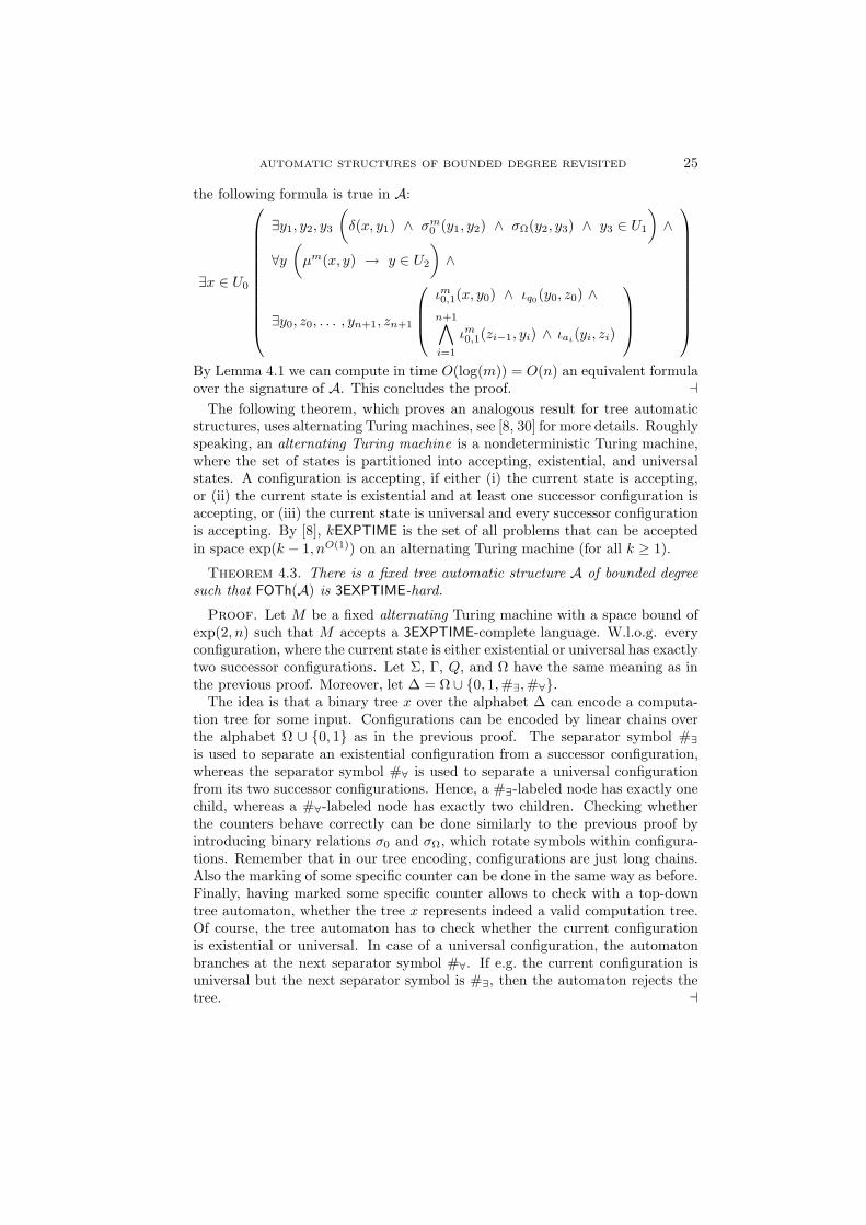
the following formula is true in A:
∃x ∈ U0
∃y1, y2, y3(
δ(x, y1) ∧ σm0 (y1, y2) ∧ σΩ(y2, y3) ∧ y3 ∈ U1
)
∧
∀y(
µm(x, y) → y ∈ U2
)
∧
∃y0, z0, . . . , yn+1, zn+1
ιm0,1(x, y0) ∧ ιq0(y0, z0) ∧n+1∧
i=1
ιm0,1(zi−1, yi) ∧ ιai(yi, zi)
By Lemma 4.1 we can compute in time O(log(m)) = O(n) an equivalent formulaover the signature of A. This concludes the proof. ⊣
The following theorem, which proves an analogous result for tree automaticstructures, uses alternating Turing machines, see [8, 30] for more details. Roughlyspeaking, an alternating Turing machine is a nondeterministic Turing machine,where the set of states is partitioned into accepting, existential, and universalstates. A configuration is accepting, if either (i) the current state is accepting,or (ii) the current state is existential and at least one successor configuration isaccepting, or (iii) the current state is universal and every successor configurationis accepting. By [8], kEXPTIME is the set of all problems that can be acceptedin space exp(k − 1, nO(1)) on an alternating Turing machine (for all k ≥ 1).
Theorem 4.3. There is a fixed tree automatic structure A of bounded degreesuch that FOTh(A) is 3EXPTIME-hard.
Proof. Let M be a fixed alternating Turing machine with a space bound ofexp(2, n) such that M accepts a 3EXPTIME-complete language. W.l.o.g. everyconfiguration, where the current state is either existential or universal has exactlytwo successor configurations. Let Σ, Γ, Q, and Ω have the same meaning as inthe previous proof. Moreover, let ∆ = Ω ∪ 0, 1,#∃,#∀.
The idea is that a binary tree x over the alphabet ∆ can encode a computa-tion tree for some input. Configurations can be encoded by linear chains overthe alphabet Ω ∪ 0, 1 as in the previous proof. The separator symbol #∃is used to separate an existential configuration from a successor configuration,whereas the separator symbol #∀ is used to separate a universal configurationfrom its two successor configurations. Hence, a #∃-labeled node has exactly onechild, whereas a #∀-labeled node has exactly two children. Checking whetherthe counters behave correctly can be done similarly to the previous proof byintroducing binary relations σ0 and σΩ, which rotate symbols within configura-tions. Remember that in our tree encoding, configurations are just long chains.Also the marking of some specific counter can be done in the same way as before.Finally, having marked some specific counter allows to check with a top-downtree automaton, whether the tree x represents indeed a valid computation tree.Of course, the tree automaton has to check whether the current configurationis existential or universal. In case of a universal configuration, the automatonbranches at the next separator symbol #∀. If e.g. the current configuration isuniversal but the next separator symbol is #∃, then the automaton rejects thetree. ⊣

26 DIETRICH KUSKE AND MARKUS LOHREY
The proof of the next result is in fact a simplification of the proof of Theo-rem 4.2, since we do not need counters.
Theorem 4.4. There is a fixed string automatic structure A of bounded degreeand polynomial growth (in fact linear growth) such that FOTh(A) is EXPSPACE-hard.
Proof. Let M be a fixed Turing machine with a space bound of 2n suchthat M accepts an EXPSPACE-complete language. Let Σ, Γ, Q, q0, qf , 2,and Ω have the usual meaning. Let ∆ = # ∪ Ω. This time, for m ∈ N,an accepting m-computation is a string x1#x2# · · ·xn#, where x1, . . . , xn ∈Γ∗QΓ+ are configurations with |xi| = m (1 ≤ i ≤ n), xi ⊢M xi+1 (1 ≤ i < n),x1 ∈ q0Σ
∗2
∗, and xn ∈ Γ∗qfΓ+. Let U0 be the fixed regular language
U0 = (Γ∗QΓ+#)+ ∩ q0Σ∗2
∗#∆∗ ∩ ∆∗qf (∆ \ #)∗# .
The following binary relations δ and σΩ can be easily recognized by 2-dimensionalautomata:
δ = (w, w ⊗ w) | w ∈ U0σΩ = (av ⊗ w, va⊗ w) | w ∈ U0, a ∈ Ω, v ∈ ∆∗
Moreover, let U1 be the following regular language over ∆∗ ⊗ ∆∗:
U1 = #u⊗v# | u, v ∈ Ω+, |u| = |v|, v ⊢M u+#u⊗v# | u, v ∈ Ω+, |u| = |v| .Then, for every x ∈ U0 and m ∈ N we have: x is an accepting m-computationif and only if there exist y1, y2 ∈ ∆∗ ⊗ ∆∗ such that δ(x, y1), σ
mΩ (y1, y2), and
y2 ∈ U1.Let us now fix some input w = a1 · · ·an ∈ Σ∗ with |w| = n, let an+1 = 2, and
let m = 2n. Thus, w is accepted by M if and only if there exists an acceptingm-computation x such that in the first configuration of x, the tape content isof the form w2
+. It remains to add some structure that allows us to expressthe latter by a formula. This can be done similarly to the proof of Theorem 4.2:Let Π = ∆ ∪ ⊲, where ⊲ is a new symbol and define the binary relations ιa(a ∈ Σ ∪ 2) as follows:
ιa = (q0av, q0a⊲v) | v ∈ ∆∗, q0av ∈ U0 ∪ (u⊲av, ua⊲v) | u, v ∈ ∆∗, uav ∈ U0Then, A = (Π∗∪(∆∗⊗∆∗), δ, σΩ, (ιa)a∈Σ∪2, U0, U1) is a fixed string automaticstructure of bounded degree and linear growth. For the latter note that theGaifman graph of A is just a disjoint union of cycles and finite paths (in fact,every node has degree at most 2). Moreover, w is accepted by M if and only ifthe following statement is true in A:
∃x ∈ U0
∃y1, y2(
δ(x, y1) ∧ σmΩ (y1, y2) ∧ y2 ∈ U1
)
∧
∃y0, . . . , yn
(
ιa1(x, y0) ∧n∧
i=1
ιai(yi−1, yi)
)
. (15)
By Lemma 4.1 this concludes the proof. ⊣The next result can be easily shown by combining the techniques from the
proof of Theorem 4.3 and 4.4. We leave the details for the reader.

AUTOMATIC STRUCTURES OF BOUNDED DEGREE REVISITED 27
Theorem 4.5. There is a fixed tree automatic structure A of bounded degreeand polynomial growth (in fact linear growth) such that FOTh(A) is 2EXPTIME-hard.
§5. Bounded quantifier alternation depth. In this section we prove somefacts about first-order fragments of fixed quantifier alternation depth. Theseresults will follow easily from the constructions in the preceding section. RecallTheorem 2.7 and 2.9 on the complexity of Σn-FOMC(SA) and Σn-FOMC(TA),respectively. These results are not restricted to structures of bounded degree.From our construction in the proof of Theorem 4.4, we can slightly sharpen thelower bound from Theorem 2.7 for n = 0.
Theorem 5.1. There exists a fixed string automatic structure of bounded de-gree and linear growth with a PSPACE-complete Σ1-theory.
Proof. Let M be a fixed linear bounded automaton with a PSPACE-completeacceptance problem and consider the structure A from the proof of Theorem 4.4.If we replace the number m in the formula (15) by n + 1, where n is the inputlength, then (15) is equivalent to the following formula, which is equivalent to aΣ1-formula:
∃x ∈ U0
∃y0, . . . , yn+2
(
δ(x, y0) ∧n+1∧
i=0
σΩ(yi, yi+1) ∧ yn+2 ∈ U1
)
∧
∃y1, . . . , yn
(
ιa1(x, y1) ∧n∧
i=2
ιai(yi−1, yi)
)
.
This formula is true in A if and only if the linear bounded automaton acceptsthe input w = a1 · · · an. ⊣
Let us now move on to Σ2-formulas and structures of arbitrary growth:
Theorem 5.2. There is a fixed string automatic structure of bounded degreewith an EXPSPACE-complete Σ2-theory.
Proof. We reuse our construction from the proof of Theorem 4.2. We startwith an exp(1, n)-space-bounded machineM that accepts an EXPSPACE-completelanguage. We carry out the same construction as in the proof of Theorem 4.2,but replace 2m (resp. m) everywhere by m (resp. the input length n). In addi-tion, we need the following (trivial) analogue of Lemma 4.1: Let the signatureS contain a binary symbol r. From a given number n (encoded unary), we canconstruct in linear time a Σ1-formula r(n)(x, y) such that for every S-structureA and all elements a, b ∈ A we have: (a, b) ∈ rn if and only if A |= r(n)(a, b).
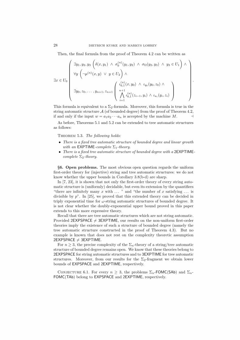
28 DIETRICH KUSKE AND MARKUS LOHREY
Then, the final formula from the proof of Theorem 4.2 can be written as
∃x ∈ U0
∃y1, y2, y3(
δ(x, y1) ∧ σ(n)0 (y1, y2) ∧ σΩ(y2, y3) ∧ y3 ∈ U1
)
∧
∀y(
¬µ(n)(x, y) ∨ y ∈ U2
)
∧
∃y0, z0, . . . , yn+1, zn+1
ι(n)0,1 (x, y0) ∧ ιq0 (y0, z0) ∧
n+1∧
i=1
ι(n)0,1 (zi−1, yi) ∧ ιai
(yi, zi)
.
This formula is equivalent to a Σ2-formula. Moreover, this formula is true in thestring automatic structure A (of bounded degree) from the proof of Theorem 4.2,if and only if the input w = a1a2 · · · an is accepted by the machine M . ⊣
As before, Theorems 5.1 and 5.2 can be extended to tree automatic structuresas follows:
Theorem 5.3. The following holds:
• There is a fixed tree automatic structure of bounded degree and linear growthwith an EXPTIME-complete Σ1-theory.
• There is a fixed tree automatic structure of bounded degree with a 2EXPTIME-complete Σ2-theory.
§6. Open problems. The most obvious open question regards the uniformfirst-order theory for (injective) string and tree automatic structures: we do notknow whether the upper bounds in Corollary 3.8(b-d) are sharp.
In [7, 23], it is shown that not only the first-order theory of every string auto-matic structure is (uniformly) decidable, but even its extension by the quantifiers“there are infinitely many x with . . . ” and “the number of x satisfying . . . isdivisible by p”. In [25], we proved that this extended theory can be decided intriply exponential time for ω-string automatic structures of bounded degree. Itis not clear whether the doubly-exponential upper bound proved in this paperextends to this more expressive theory.
Recall that there are tree automatic structures which are not string automatic.Provided 2EXPSPACE 6= 3EXPTIME, our results on the non-uniform first-ordertheories imply the existence of such a structure of bounded degree (namely thetree automatic structure constructed in the proof of Theorem 4.3). But noexample is known that does not rest on the complexity theoretic assumption2EXPSPACE 6= 3EXPTIME.
For n ≥ 3, the precise complexity of the Σn-theory of a string/tree automaticstructure of bounded degree remains open. We know that these theories belong to2EXPSPACE for string automatic structures and to 3EXPTIME for tree automaticstructures. Moreover, from our results for the Σ2-fragment we obtain lowerbounds of EXPSPACE and 2EXPTIME, respectively.
Conjecture 6.1. For every n ≥ 3, the problems Σn-FOMC(SAb) and Σn-FOMC(TAb) belong to EXPSPACE and 2EXPTIME, respectively.

AUTOMATIC STRUCTURES OF BOUNDED DEGREE REVISITED 29
A possible attack to this conjecture would follow the line of argument in theproof of Theorem 3.7 and would therefore be based on Gaifman’s theorem. Tomake this work, the exponential bound in Gaifman’s theorem would have to bereduced which leads to the following conjecture.
Conjecture 6.2. Let A be a structure, (a1, . . . , ak), (b1, . . . , bk) ∈ Ak, d ≥n ≥ 0, and D1, . . . , Dk ≥ d · 2n such that
(A(
k⋃
i=1
S(Di, ai)), a1, . . . , ak) ≃ (A(
k⋃
i=1
S(Di, bi)), b1, . . . , bk) .
Then, for every Σn-formula ϕ(x1, . . . , xk) of quantifier depth at most d, we have:
A |= ϕ(a1, . . . , ak) ⇐⇒ A |= ϕ(b1, . . . , bk) . (16)
Gaifman’s Theorem 3.1 implies that the conclusion (16) holds, if the lowerbound d · 2n for the radius is replaced by 2d. The intuition behind this con-jecture is that quantifier alternation (and not only nesting of quantifiers of thesame type) seems to be essential in order to express exponential distances in theGaifman-graph (see also the proof of Lemma 4.1).
REFERENCES
[1] V. Barany, Invariants of automatic presentations and semi-synchronous transductions,Proceedings of STACS’06, Lecture Notes in Computer Science vol. 3884, Springer, 2006,pp. 289–300.
[2] , Automatic presentations of in
nite structure, Ph.D. thesis, RWTH Aachen, 2007.[3] V. Barany, E. Gradel, and S. Rubin, Automata-based presentations of infinite struc-
tures, 2010.[4] V. Barany, L. Kaiser, and S. Rubin, Cardinality and counting quantifiers on omega-
automatic structures, Proceedings of STACS’08, IFIB Schloss Dagstuhl, 2008, pp. 385–396.[5] M. Benedikt, L. Libkin, Th. Schwentick, and L. Segoufin, Definable relations and
first-order query languages over strings, J. ACM, vol. 50 (2003), no. 5, pp. 694–751.[6] A. Blumensath, Automatic structures, Diploma Thesis, RWTH Aachen, 1999.[7] A. Blumensath and E. Gradel, Automatic Structures, Proceedings of LICS’00, IEEE
Computer Society Press, 2000, pp. 51–62.[8] A. K. Chandra, D. C. Kozen, and L. J. Stockmeyer, Alternation, J. ACM, vol. 28
(1981), no. 1, pp. 114–133.[9] Th. Colcombet and Ch. Loding, Transforming structures by set interpretations,
Log. Methods Comput. Sci., vol. 3 (2007), pp. 1–36.[10] H. Comon, M. Dauchet, R. Gilleron, C. Loding, F. Jacquemard, D. Lugiez,
S. Tison, and M. Tommasi, Tree automata techniques and applications, Available on: http:
//www.grappa.univ-lille3.fr/tata, 2007, Release October, 12th 2007.[11] K.J. Compton and C.W. Henson, A uniform method for proving lower bounds on the
computational complexity of logical theories, Ann. Pure Appl. Logic, vol. 48 (1990), pp. 1–79.[12] A. Dawar, M. Grohe, St. Kreutzer, and N. Schweikardt, Model theory makes
formulas large, Proceedings of ICALP 2007, Lecture Notes in Computer Science vol. 4596,Springer, 2007, pp. 913–924.
[13] Ch. Delhomme, V. Goranko, and T. Knapik, Automatic linear orderings, Manu-script, 2003.
[14] C.C. Elgot, Decision problems of finite automata design and related arithmetics,Trans. Amer. Math. Soc., vol. 98 (1961), pp. 21–51.

30 DIETRICH KUSKE AND MARKUS LOHREY
[15] D.B.A. Epstein, J.W. Cannon, D.F. Holt, S.V.F. Levy, M.S. Paterson, andW.P. Thurston, Word processing in groups, Jones and Bartlett Publishers, Boston, 1992.
[16] H. Gaifman, On local and nonlocal properties, Logic colloquium ’81 (J. Stern, editor),North-Holland, 1982, pp. 105–135.
[17] G. Hjorth, B. Khoussainov, A. Montalban, and A. Nies, From automatic structures
to Borel structures, Proceedings of LICS’08, IEEE Computer Society, 2008, pp. 431–441.[18] B.R. Hodgson, On direct products of automaton decidable theories, Theoret. Com-
put. Sci., vol. 19 (1982), pp. 331–335.[19] I. Ishihara, B. Khoussainov, and S. Rubin, Some results on automatic structures,
Proceedings of LICS’02, IEEE Computer Society Press, 2002, pp. 235–244.[20] B. Khoussainov and A. Nerode, Automatic presentations of structures, Logic and
computational complexity, Lecture Notes in Comp. Science vol. 960, Springer, 1995, pp. 367–392.
[21] B. Khoussainov and S. Rubin, Graphs with automatic presentations over a unary
alphabet, J. Autom. Lang. Comb., vol. 6 (2001), pp. 467–480.[22] B. Khoussainov, S. Rubin, and F. Stephan, On automatic partial orders, Proceed-
ings of LICS’03, IEEE Computer Society Press, 2003, pp. 168–177.[23] , Definability and regularity in automatic structures, Proceedings of
STACS’04, Lecture Notes in Comp. Science vol. 2996, Springer, 2004, pp. 440–451.[24] D. Kuske, Is Cantor’s theorem automatic?, Proceedings of LPAR’03, Lecture Notes
in Comp. Science vol. 2850, Springer, 2003, pp. 332–345.[25] D. Kuske and M. Lohrey, First-order and counting theories of ω-automatic struc-
tures, this Journal, vol. 73 (2008), pp. 129–150.[26] D. Kuske, Theories of automatic structures and their complexity, Proceedings of
CAI’09, Lecture Notes in Computer Science vol. 5725, 2009, pp. 81–98.[27] D. Kuske and M. Lohrey, Some natural decision problems in automatic graphs, this
Journal, vol. 75 (2010), no. 2, pp. 678–710.[28] M. Lohrey, Automatic structures of bounded degree, Proceedings of LPAR’03, Lec-
ture Notes in Comp. Science vol. 2850, Springer, 2003, pp. 344–358.[29] A.R. Meyer, Weak monadic second order theory of one successor is not elementary
recursive, Proc. Logic colloquium, Lecture Notes in Mathematics vol. 453, Springer, 1975,pp. 132–154.
[30] C. H. Papadimitriou, Computational complexity, Addison Wesley, 1994.[31] S. Rubin, Automata presenting structures: A survey of the finite string case, The
Bulletin of Symbolic Logic, vol. 14 (2008), pp. 169–209.[32] H. Seidl, Single-valuedness of tree transducers is decidable in polynomial time, The-
oret. Comput. Sci., vol. 106 (1992), pp. 135–181.[33] P. V. Silva and B. Steinberg, A geometric characterization of automatic monoids,
Q. J. Math., vol. 55 (2004), pp. 333–356.[34] A. Weber, On the valuedness of finite transducers, Acta Inform., vol. 27 (1990),
pp. 749–780.[35] Th. Weidner, Die Große injektiver baumautomatischer Darstellungen und die Kom-
plexitat ihrer Berechnung, Diploma thesis, University of Leipzig, 2010, in German, Englishversion in preparation.
TECHNISCHE UNIVERSITAT ILMENAU
INSTITUT FUR THEORETISCHE INFORMATIK
ILMENAU, GERMANY
E-mail : [email protected]
UNIVERSITAT LEIPZIG
INSTITUT FUR INFORMATIK
LEIPZIG, GERMANY
E-mail : [email protected]