Automatic Solution of Jigsaw Puzzles

Daniel J. Hoff1 Peter J. Olver1

Department of Mathematics School of MathematicsUniversity of California, San Diego University of MinnesotaLa Jolla, CA 92093 Minneapolis, MN 55455d1hoff@math.ucsd.edu olver@math.umn.edu

http://www.math.umn.edu/∼olver

Abstract

We present a method for automatically solving apictorial jigsaw puzzles that is basedon an extension of the method of differential invariant signatures. Our algorithmsare designed to solve challenging puzzles, without having to impose any restrictiveassumptions on the shape of the puzzle, the shapes of the individual pieces, or theirintrinsic arrangement. As a demonstration, the method was successfully used to solvetwo commercially available puzzles. Finally we perform some preliminary investigationsinto scalability of the algorithm for even larger puzzles.

Keywords:jigsaw puzzle, curvature, Euclidean signature, bivertex arc, piece fitting, piece locking

1 Introduction.

In this paper, we present a new algorithm for the automatic solution of apictorial jigsawpuzzles, meaning that there is no design or picture and the solution requires matching onlythe shapes of the individual pieces, cf. [10]. Our method is founded on the extended Euclideansignature method for object recognition and curve matching that we developed in [16]. Weillustrate its efficacy by automatically solving two commercially available jigsaw puzzles: TheRain Forest Giant Floor Puzzle, [23], has fairly standard shaped pieces and is relatively easyto solve by hand, especially if one also uses the puzzle picture to guide in placement of thepieces. The Baffler Nonagon, [33], is considerably more challenging, as it is truly apictorial,with very irregularly shaped pieces, each of a distinct textured color.

The initial step in our procedure is to accurately photograph the puzzle pieces, in randomorientations, which are then presented to the computer in the form of JPEG digital images.Following segmentation and smoothing of the boundary curves of each piece, the algorithmapplies invariant numerical algorithms, [1, 4] to calculate the two simplest Euclidean differen-tial invariants — the curvature and its derivative with respect to arc length — that are usedto parametrize the Euclidean signature curve. A fundamental theorem, [4, 20], states thattwo sufficiently regular plane curves are equivalent under a rigid motion if and only if they

1Supported in part by NSF Grant DMS 08–07317.

1

have identical Euclidean signatures. An important feature is that, unlike, say, characterizingcurves via curvature as a function of arc length, [15], such differential invariant signatures arefully local, and hence can be readily adapted both to curves under occlusion, and to puzzlepieces where one only matches a part of the boundary curves. The extension developed in[16] breaks up the complete signatures into subarcs, which corresponds to a decompositionof the original curves into “bivertex arcs” (see Section 2 for definitions). Individual bivertexarcs with the same signature are then matched by rigid motions; if these all agree, the curvesare rigidly equivalent.

A key feature is that our algorithms rely solely on the shapes of the puzzle pieces, and noton any picture or design which may appear thereon. (At the opposite end of the spectrumare algorithms that deal solely with image information, on puzzles with all square pieces,[12].) It is worth emphasizing that our method is founded upon the characterization of the(approximate) bivertex arcs of the puzzle boundaries, which in turn are characterized throughthe two curvature invariants used to construct the differential invariant signature. With thebivertex arc signatures already known, we can efficiently compare them to determine potentialfits between puzzle pieces, which are then refined using a new method we call “piece locking”.With some tuning of the parameters used in the various components, the resulting methodis remarkably accurate and able to automatically solve large scale, challenging, commercialpuzzles.

While of limited practical use, at least outside the entertainment world, puzzle assemblyhas been studied with a number of more important applications in mind. In [18, 24], forinstance, puzzle solution techniques are applied to broken tiles to simulate the reconstructionof archaeological artifacts. In fall, 2011, DARPA held a competition, with a $50,000 prize,to automatically reconstruct a collection of shredded documents, [8]. Recreational solvingof jigsaw puzzles belongs to the class of problems for which humans have a natural aptitudebut automation remains considerably more challenging. This is especially true of puzzlesthat combine to form a picture, in which case human solution is typically more a matterof patience than mental exertion. Because of this natural motivation, much previous work,e.g., [13, 30, 32], has focused on solving archetypical jigsaw puzzles, whose overall form isconstrained by several rather restrictive assumptions, the most common being:

(1) The individual pieces have four well-defined sides, each of which contains either an “in-dent” or an “outdent”.

(2) Each piece has at most four primary neighbors, one on each side (except, of course, forpieces on the puzzle boundary) that are fitted together via the “indents” and “outdents”.

(3) The solved puzzle has pieces positioned on an (approximate) grid.

(4) The boundary of the solved puzzle is an easily identified smooth shape, e.g., a rectangle.

For example, the algorithm proposed in [34] employs bitangents and distinguished pointsto match simple “indents” and “outdents”, and relies heavily on recognizing the boundaryand corner pieces to start the assembly process. Using all four assumptions, two intermixed104-piece puzzles were solved in [30]. A more recent work, [13], solves a 204-piece puzzle,where adjacent pieces are matched by comparing ellipses fitted to the “indents” and “out-dents”. However, the algorithms developed in [13, 30, 34] will not extend to more challenging

2

situations such as the Baffler Nonagon puzzle, shredded documents, or broken ceramics re-construction, where none of these simplifying assumptions hold.

Our goal is to develop a method of puzzle assembly that does not require any of as-sumptions (1–4), and therefore can be readily extended beyond the realm of standard jigsawpuzzles. We do impose a mild restriction that the puzzle pieces have smooth boundary curves,of class at least C3, that are also “v-regular”, in the terminology of [16]. The latter technicalassumption is defined below, and, being purely mathematical, is automatically satisfied inpractical applications. One might, however, justifiably question our smoothness assumption,as many physical puzzle pieces, as well as pieces of broken pottery and tiles, have corners.Despite this limitation, in practice we are able to successfully deal with puzzle pieces withcorners by applying a preliminary curve smoothing procedure that slightly rounds them off,and this has sufficed in all the examples we have tested the algorithm on. Indeed, whenthe images of the puzzles pieces are coarsely digitized, a preliminary smoothing step is es-sential for accurate computation of the required Euclidean signatures. Competing generalalgorithms can be found in [10], which focusses on the types of “junctions”, where three ormore pieces touch, [22], which bases curve matching on polar coordinate systems centeredaround vertices of their boundaries, i.e., local extrema of the curvature, and [18], which usesdynamic programming methods to match the curvature and arc length invariants of pairs ofpieces, and then refines the result by matching piece triples.

Our approach to fitting puzzle pieces together is based on two principal tools. First,we note that the problem of matching individual piece boundaries is closely related to therecognition of planar objects under rigid motions. Based on Elie Cartan’s solution to theequivalence problem for submanifolds under general Lie group actions, cf. [20], the use ofdifferential invariant signature curves for planar object recognition was promoted in [4], andthen extended to cover more general cases in [16]. The extended invariant signature methodnaturally lends itself to puzzle solving since it decomposes boundary curves into bivertexarcs, as defined below, thereby readily allowing one to compare parts of piece boundaries. InSubsection 5.1, we adapt the ideas of [16] to formulate an algorithm for finding possible piece-to-piece fits. An important point is that the piece fitting algorithm concentrates exclusivelyon the bivertex arcs, and hence ignores any straight line segments and circular arcs appearingin the piece boundaries. In particular, this approach frees our algorithm from reliance onthe existence of a rectangular or other prescribed boundary of the entire puzzle; indeed, theboundary pieces tend to be among the last to be placed during the assembly process.

The second tool was developed after we recognized a need to increase the quality andconfidence with which pieces are placed. This is desirable not only because it maximizesthe overall solution confidence, but also because it minimizes the need for back-tracking andbranching, allowing for larger puzzles to be successfully solved. When humans correctly placea jigsaw puzzle piece, they are rewarded with a noticeable feeling of it “snapping” into place.Moreover, it is shown in [3] that for robotic puzzle assembly, monitoring the feedback forcecan be a useful simulation of this sensation. In Subsection 5.2, we develop a method ofpiece locking, which is designed as a computational analogue of this feeling and based on themagnitude of a fictitious electrostatic force and torque between matching piece boundaries.

In the penultimate section, we apply our method to two commercially available puzzles,[23, 33]. Accurate photos of the individual puzzle pieces were segmented using a standardsnake algorithm, [6, 7, 17]. The resulting contours were then subjected to a preliminary

3

smoothing using a naıve spline algorithm. After the preprocessing step, the piece fitting andlocking algorithms were run until completion. Unlike most previous puzzle solving algorithms,ours work from the “inside out”; in other words, the initially selected piece tends to belocated inside the puzzle, not on its boundary, and the subsequent pieces are successivelyfitted together, building the puzzle up from its interior, and avoiding any need to identifyboundary pieces as such. With appropriate choices of adjustable parameters, effectivelybalancing processing speed versus accuracy of the piece placements, the Rainforest and Bafflerpuzzles were successfully solved in, respectively, 58 and 31 minutes on an Intel R© CoreTM 2Duo E8500 3.17GHz processor.

The final section presents some preliminary investigations into scalability of our algorithmto even larger puzzles. The Cathedral jigsaw puzzle [29], is a non-standard 1000 piece puzzle,yet its individual pieces contain many standard “indents” and “outdents.” This combinationmakes it particularly challenging, since there are many “local” near-matches, and yet sim-plified algorithms designed for standard puzzles cannot be applied because of the unusualstructure. While we have not, as yet, achieved complete success in this much more chal-lenging situation, the algorithm did successfully assemble 103 pieces of a 111 piece subpuzzlebefore terminating, in approximately 36 hours. If we had a similar sized puzzle with moreirregular pieces, as in the Baffler, we would expect much greater success. Thus, while furtherwork remains to be done, our conclusion is that the algorithm does lend itself to applicabilityto much larger puzzles and is eminently scalable.

2 Curves and Puzzles.

Let us introduce our basic terminology and assumptions, based on that used in [15, 16]. Wewill be working exclusively with plane puzzles. (Extending our methods to three-dimensionalpuzzles, e.g., a broken statue, would be an interesting challenge. While the mathematicalmachinery is in place, [20], their practical implementation remains daunting.) We will workin the Euclidean plane with the standard norm, denoted ‖ z ‖ =

√x2 + y2 for z = (x, y) ∈

R2. We let SE(2) denote the three-dimensional special Euclidean group consisting of allorientation-preserving isometries, or rigid motions :

z 7−→ Rz + c, z =

(xy

)∈ R2, where R =

(cos θ − sin θsin θ cos θ

), c =

(ab

), (2.1)

are, respectively, a 2 × 2 matrix representing rotation through angle θ and a translationvector. We will consistently identify planar objects up to rigid motion. All curves C ⊂ R2

are assumed to be compact, rectifiable — and hence of finite length — and simple, i.e.,without self-intersections. A closed curve is called a Jordan curve, while a non-closed curve,with distinct endpoints, will be called an arc. Two arcs are said to be non-overlapping if theyhave at most one or both endpoints in common.

By definition, a puzzle piece is a bounded, simply connected plane domain P ⊂ R2 whoseboundary C = ∂P is a Jordan curve of class C3. Two puzzle pieces P, P are congruent, andhence considered to be the same, if they are rigidly equivalent, meaning that there is a rigidmotion g ∈ SE(2) such that P = g · P. Two puzzle pieces P, P are said to fit together if they

share a common arc S = P ∩ P = ∂P ∩ ∂P, or, more generally, if they do so after a rigid

4

motion: S = P ∩ (g ·P) = ∂P ∩ (g ·∂P) for some g ∈ SE(2). Keep in mind that pieces that fitdo not overlap. In practice, the shared arc should not be too short, although this requirementneed not be directly quantified as it will follow as a consequence of our fitting and lockingalgorithms. We can also allow two puzzle pieces to fit along more than one connected arc,although this is uncommon in real world puzzles. It is also not difficult to allow non-simplyconnected puzzle pieces, again rare in examples.

Remark: The key assumption used in this work is that the puzzle pieces are smooth (ofclass C3), and hence do not have corners. Clearly, many physical puzzles contain pieces withcorners, and it would be worth directly adapting our algorithms to cover such pieces. Suchan extension will not be difficult; indeed, during the course of the assembly process, we dealwith subpuzzles, that is, unions of puzzle pieces, whose boundary is only piecewise C3 (andnot necessarily simply connected). However, this adaption has proven to be unnecessary forthe practical solution of all the puzzles we have tried, since the digital images of the puzzlepieces must be subjected to a preliminary smoothing operation anyways before the assemblyalgorithm can proceed.

By an apictorial puzzle, or puzzle for short, we mean a bounded plane domain P ⊂ R2

that is the union,

P =n⋃i=1

(gi · Pi), (2.2)

of individual puzzle pieces Pi subject to rigid motions gi ∈ SE(2), which we sometimesrefer to as placements. We suppose that any two pieces, when placed, are either disjoint,(gi ·Pi) ∩ (gj ·Pj) = ∅, or touch at a single point1 {z0 } = (gi ·Pi) ∩ (gj ·Pj), or fit togetheraccording to the preceding definition. However, while standard jigsaw puzzles satisfy this,our algorithms don’t actually require this assumption to hold, and so could, in principle,solve “multi-layered puzzles”, whose pieces are allowed to overlap. (While this strikes us asan intriguing extension of standard jigsaw puzzles, we are not aware of any actual examples.)In the puzzle assembly problem, we are given the pieces P∗ = {P1, . . . ,Pn}, and our task is todetermine the corresponding rigid motions g1, . . . , gn required to assemble P . Our methodswork best when pieces that fit together do so uniquely, and only fit in accordance with theirpositions in the final puzzle assembly. However, more sophisticated backtracking techniquescould be developed to better deal with non-uniqueness of fits (e.g., as in [18]).

3 Equivalence of Curves.

Our algorithm for fitting puzzle pieces together is based on the solution to the equivalenceproblem for plane curves based on extended Euclidean-invariant signatures developed in [16].Let us review the key points, leaving the complete details to the aforementioned reference.

Given a C3 Jordan curve C ⊂ R2, let z(s), 0 ≤ s ≤ L, denote its arc length paramet-rization, so that L is the length of C and z(s) is periodic of period L. Let κ(s) denote thesigned curvature at the point z(s) ∈ C, and κs(s) = dκ/ds its derivative with respect to arc

1More generally, one can allow pieces to touch at a finite number of points, although this is uncommonin real world examples.

5

length. Note that both κ and κs are Euclidean differential invariants, meaning that they areunaffected by rigid motions, [20].

A point z(s) ∈ C is called regular if κs(s) 6= 0. An ordinary vertex is a local extremumof curvature, [15]. We define a generalized vertex to be maximal connected arc V ⊂ C onwhich κs(s) ≡ 0. Thus, a generalized vertex is either an ordinary vertex, or a critical point ofcurvature, or a circular arc, or a straight line segment. In this paper, all curves are assumedto be v-regular, [16], meaning that they have only finitely many generalized vertices. Curveswith infinitely many vertices exist in theory, but are pathological and cannot arise in realworld applications.

By a bivertex arc, we mean an arc B ⊂ C that has κs = 0 at both endpoints, but all ofwhose interior points are regular. A basic result of [16] states any v-regular C3 Jordan curvethat is not a circle has a unique bivertex decomposition,

C =m⋃j=1

Bj ∪n⋃k=1

Vk, (3.1)

into a finite union of m ≥ 4 non-overlapping bivertex arcs B1, . . . , Bm, and n ≥ 0 generalizedvertices V1, . . . , Vn. Note that we exclude point vertices from the bivertex decomposition,since they are accounted for by the endpoints of the bivertex arcs Bj.

Two plane curves C, C ∈ R2 are said to be rigidly equivalent, or congruent for short, ifthere exists a rigid motion g ∈ SE(2) such that C = g ·C. We extend the notion of congruenceto disconnected unions of curves, keeping in mind that for two unions to be congruent, theirconstituent curves must be pair-wise congruent under the same rigid motion. The followingresult was established in [16].

Proposition 1. Two v-regular plane curves C, C ⊂ R2 are congruent if and only if theunions of their constituent bivertex arcs are congruent.

Using a reformulation of Cartan’s general solution to the local equivalence problem ofsubmanifolds under Lie group actions, [5], a solution to the equivalence problem for planecurves based on their Euclidean signature was proposed in [4], and subsequently applied toobject recognition and symmetry detection in a variety of contexts, [25, 26].

Definition 2. Let C be a plane curve of class C3 and of length L <∞. The Euclidean sig-nature of C is the (non-simple) plane curve S(C) = { (κ(s), κs(s)) | 0 ≤ s ≤ L } parametrizedby the curvature and its derivative with respect to arc-length.

The following theorem is a consequence of Proposition 1, combined with general resultson group-invariant signatures2 of regular submanifolds, [20].

Theorem 3. Let C, C ⊂ R2 be v-regular, non-circular Jordan curves whose bivertex decom-positions contain the same number, n, of non-overlapping bivertex arcs. Assume that, foreach j = 1, . . . , n, the bivertex arcs Bj and Bj have identical signatures : S(Bj) = S(Bj),

which implies that Bj, Bj are congruent, and hence there exist rigid motions gj ∈ SE(2) such

that Bj = gj · Bj. If, in addition, all the gj = g are the same, then the entire curves are

rigidly equivalent : C = g · C.

2The older term “classifying submanifold” is used in place of “signature” in [20].

6

In practical applications, the puzzle pieces are inputted to the computer as digital imagesand then segmented to retrieve their boundaries. (See Section 6 for practical details.) Asa result, each piece is represented by a discrete set of sample points C∆ = {z1, . . . , zN},where each zj lies on or near its boundary curve C. The actual curve can be approximatelyreconstructed from C∆ by some form of interpolation, e.g., periodic splines, possibly coupledwith smoothing to reduce the effect of noise. We similarly (approximately) discretize thesignature curve S(C) by S∆ = (σ1, . . . , σN), where each point σj = (κj, κjs) ∈ S∆ consistsof suitable numerical approximations to the curvature and its arc length derivative at thecorresponding sample point zj = (xj, yj) ∈ C∆. For example, the entries of σj may befound directly from the discretized curve C∆ by employing the Euclidean-invariant numericalapproximations to the curvature invariants developed in [1, 4].

According to the algorithm developed in [16], to determine if two discretized curves arerigidly equivalent, the first step is to construct their (approximate) bivertex decompositionsby splitting each curve into subarcs whenever |κs | − δ0 changes sign, where δ0 > 0 is a fixedsmall cut-off. In order to achieve more consistent approximate Bivertex Arc Decompositions,we additionally split curves wherever |κs| achieves a local minimum, provided that minimumexceeds the parameter δ0. This added convention helps to reduce sensitivity to the valueof δ0. Additionally, instead of eliminating insignificant arcs over which curvature changesby less than δ1 (as in [16]), we eliminate arcs on which the maximum of |κ| is less than δ1.Details on the selection of δ0 and δ1 are presented in [16], though we note that in this paper

the quantity Dκ(C, C) therein is taken as a maximum over all inputed pieces (rather thanjust two), and is denoted dκ.

The next step is to compare individual (discrete) bivertex arcs using their (discrete) Eu-clidean signatures. The method, developed in detail in [16], is based, roughly, on the idea ofregarding the discrete signatures as two collections of oppositely charged points, and deter-mining the mutual electrostatic attraction, [31]. (Or, equivalently, their mutual gravitationalattraction as point masses.) After some manipulation, we determine a signature similarity

coefficient p(B, B) ∈ [0, 1] that serves to measure the closeness of two individual bivertex arc

signatures, where a score of 1 reflects identical signatures, while p(B, B) decreases to 0 as thesignatures become increasingly disparate, and hence the arcs less and less likely to be con-gruent. To compare the two curves, we first construct approximate bivertex decompositions,and then ensure that they contain the same number of arcs; if not, there is a good chance thecurves are not rigidly equivalent, but this may be due to noise, even with our selection of thecut-off parameter δ0. In this case, the procedure for eliminating arcs from the larger collectionis to delete those on which the curvature changes least. Sometimes, several possible deletionsare tested. We then test the pairwise congruence of the resulting two collections of bivertexarcs, ordered as one traverses the curves with the same orientation. If they are congruent,one then checks whether the corresponding rigid motions are (approximately) identical, andif so the curves are deemed to be congruent.

4 Puzzle Assembly.

We now present the steps used in our puzzle solving algorithm. The method relies on suc-cessively fitting individual pieces by matching bivertex arcs along their boundaries and then

7

improving the fits via piece locking. The details of piece fitting and locking will appear inthe following section.

We begin with the collection of puzzle pieces, denoted P∗ = {P1, . . . ,Pn}, whose bound-aries Cj = ∂Pj are supplied as suitably segmented and smoothed (discrete) plane curves.The puzzle is solved by constructing a corresponding collection of rigid motions G∗ ={g1, . . . , gn} ⊂ SE(2) that form the completed puzzle (2.2). Without loss of generality,one of these can be fixed as the identity transformation: gi1 = e.

At each step k = 1, 2, . . . , in the algorithm, we will have already assembled a subpuzzleQk ⊂ P consisting of k pieces Q∗k = {Pi1 , . . . ,Pik } ⊂ P∗, along with the corresponding rigidmotions H∗k = {gi1 , . . . , gik } required to assemble it:

Qk =k⋃ν=1

(giν · Piν ) ⊂ P . (4.1)

Let R∗k = P∗ \ Q∗k denote the set of pieces that remain to be assembled. The algorithmterminates with either a fully assembled puzzle, with Qn = P , or, for some k < n, a subpuzzleQk ( P , for which the program is unable to fit any of the pieces remaining in R∗k .

For each 1 ≤ j ≤ n, we let B∗j = {B1, . . . , Bmj} be the set of bivertex arcs (or, moreaccurately, discrete approximate bivertex arcs) associated with the puzzle piece Pj. It willbe important to order the arcs in B∗j consecutively as the boundary Cj is traversed in acounterclockwise manner. During the assembly process, any bivertex arcs that have alreadybeen fit to neighboring pieces, after successful piece locking, are deemed to be inactive, andso not available during the subsequent fitting process. We let

V∗k ⊂k⋃ν=1

B∗iν

denote the set of active bivertex arcs for the subpuzzle Qk. In principle, V∗k should onlycontain the bivertex arcs situated on the outer boundary of Qk, although noise or otherartifacts might prevent some interior bivertex arcs from being matched and hence remainingin V∗k by “accident”. Fortunately, this does not seriously affect the performance of ouralgorithm in practical situations.

It should be noted that for the purposes of pairing bivertex arcs, each assembled pieceretains its individuality, and bivertex arcs on a piece boundary remain consecutive whetheror not they are currently active. One evident limitation is that the program doesn’t considercombinations of, say, two bivertex arcs from one assembled piece and three from an adjacentassembled piece, fitting five consecutive arcs on a not yet placed piece. On the other hand,the algorithm does use this extra information during piece locking, when the assembled sub-puzzle is treated as a single piece. While developing a way to universally treat subpuzzles assingle pieces could improve performance, it seemed unnecessary for many practical situations,including the puzzles treated here.

The first step in the assembly algorithm is to select a piece to form the initial subpuzzleQ∗1 = {Pi1 }, and, by default, set gi1 = e. The choice of starting piece is not so important.Our convention is to choose the piece that maximizes the total curvature

∑|κi |, summed

over all the points in the piece’s discretized signature, because, as argued in [16], arcs of

8

high curvature tend to “better” determine a simple closed curve. Our aim is to maximizethe chances of finding successful fits early on, by ensuring that the starting piece has manywell-defined features. Indeed, since straight lines are of minimal curvature — and also notincluded in the bivertex arcs and not candidates for fitting — this initial selection is alsomore likely to be an interior piece of the puzzle.

To continue, at each step k ≥ 1, we construct the next subpuzzle by finding an unattachedpiece Pi ∈ R∗k that fits the current subpuzzle Qk under a rigid motion gi ∈ SE(2), andthen setting Q∗k+1 = Q∗k ∪ {Pi }, G∗k+1 = G∗k ∪ {gi }. We select the piece Pi through anadaptation of the piece fitting and locking algorithms; details appear in the following section.If no suitable piece can be found, the algorithm terminates. Otherwise, the bivertex arcs thatwere deemed to be matched in the piece locking stage that attaches Pi to Qk are relabeledas inactive, and hence deleted from the collection V∗k ∪ B∗i in order to form the new set ofactive bivertex arcs V∗k+1.

Remark: A more sophisticated approach would be to allow several distinct subpuzzles tobe assembled concurrently, and then deal with the problem of fitting the subpuzzles together.This proved to be not necessary for the puzzles we tried our algorithm on.

5 Fitting Puzzle Pieces Together.

In this section, we present our algorithms for fitting and locking two individual puzzle pieces.At the end, we explain how to adapt the basic algorithms to fit and lock a piece with asubpuzzle.

As above, given two puzzle pieces P, P, by a fit, we just mean a rigid motion g ∈ SE(2).

The quality of the fit g measures how well an arc of g ·C approximates an arc of C. Findinga good fit is accomplished in two steps. First, we apply the extended Euclidean-invariantsignature method developed in [16] to form a stockpile of potential piece-to-piece fits. Fits

are ranked according to their µ(P, P) confidence scores. We then attempt to refine the fitsusing the ensuing method of piece-locking. Once a lock of sufficiently high quality is found,that piece is added to the subpuzzle.

We remark that an algorithm that relies solely on selecting fits with the highest confidencescores, without the extra refinement of piece-locking, is reasonably successful at solving smallpuzzles. However, the resulting fit transformations tend to be insufficiently accurate, andthe method can easily accumulate increasing errors that can hinder its success with largerpuzzles. Figure 1(a), for instance, shows such a solution of a nine puzzle piece fragment.While the pieces have been placed with correct adjacency, it is clear from figure 1(b) thatthe refinement provided by piece locking generates a much better solution.

This may well inspire the reader to ask why not proceed directly to piece locking andavoid the preliminary signature-based fitting procedure? The reason is efficiency: directpiece-locking method is much slower than signature comparison, especially as the curvatureinvariants comprising the signature were already been computed in order to characterize therequired bivertex arcs. Our combination of preliminary fitting followed by the more accuratelocking procedure on potential fits appears optimal for both speed and reliability.

9

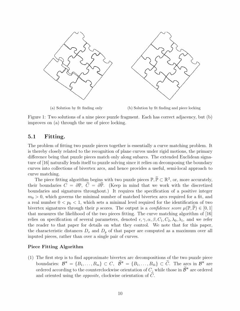
(a) Solution by fit finding only (b) Solution by fit finding and piece locking

Figure 1: Two solutions of a nine piece puzzle fragment. Each has correct adjacency, but (b)improves on (a) through the use of piece locking.

5.1 Fitting.

The problem of fitting two puzzle pieces together is essentially a curve matching problem. Itis thereby closely related to the recognition of plane curves under rigid motions, the primarydifference being that puzzle pieces match only along subarcs. The extended Euclidean signa-ture of [16] naturally lends itself to puzzle solving since it relies on decomposing the boundarycurves into collections of bivertex arcs, and hence provides a useful, semi-local approach tocurve matching.

The piece fitting algorithm begins with two puzzle pieces P, P ⊂ R2, or, more accurately,their boundaries C = ∂P, C = ∂P. (Keep in mind that we work with the discretizedboundaries and signatures throughout.) It requires the specification of a positive integerm0 > 0, which governs the minimal number of matched bivertex arcs required for a fit, anda real number 0 < p0 < 1, which sets a minimal level required for the identification of twobivertex signatures through their p scores. The output is a confidence score µ(P, P) ∈ [0, 1]that measures the likelihood of the two pieces fitting. The curve matching algorithm of [16]relies on specification of several parameters, denoted ε, γ, α, β, C1, C2, λ0, λ1, and we referthe reader to that paper for details on what they control. We note that for this paper,the characteristic distances Dx and Dy of that paper are computed as a maximum over allinputed pieces, rather than over a single pair of curves.

Piece Fitting Algorithm

(1) The first step is to find approximate bivertex arc decompositions of the two puzzle piece

boundaries: B∗ = {B1, . . . , Bm} ⊂ C, B∗ = {B1, . . . , Bm} ⊂ C. The arcs in B∗ are

ordered according to the counterclockwise orientation of C, while those in B∗ are orderedand oriented using the opposite, clockwise orientation of C.

10

(2) For each pair of bivertex arcs B ∈ B∗ and B ∈ B∗, compute their signature similarity

coefficient p(B, B) ∈ [0, 1] using the procedure presented in [16].

(3) Find maximal sequences of m + 1 ≥ m0 consecutive bivertex arcs {Bi, . . . , Bi+m} ⊂ B∗and {Bj, . . . , Bj+m} ⊂ B∗ that satisfy p(Bi+l, Bj+l) ≥ p0 for all 0 ≤ l ≤ m.

(4) If no suitable pairs of sequences exist, set µ(P, P) = 0. Otherwise, for each such pair,

use the method3 of [16] to approximate the transformations gk that takes Bi+k to Bj+k,

and calculate the associated µ(P, P) score. As in (2.1), we represent each rigid motiongk by its parameters (θk, ak, bk) ∈ S1 ×R2. The algorithm then returns the rigid motiongfit = (θfit , afit , bfit), whose parameters are obtained by simply averaging4

θfit = arg

(m∑k=1

ei θk

), afit = mean {ak}, bfit = mean {bk}, (5.1)

as a possible piece-to-piece fit with confidence score µ(P, P).

5.2 Locking.

Piece locking quantifies the physical sensation a puzzle assembler experiences when two piecesare successfully fit together. Our simulation of this feeling will be based on the generalizedelectrostatic/gravitational attractive force that was used to compare signatures in [16], andhence underlies our computation of the p scores used in the piece fitting algorithm of the pre-ceding subsection. In the locking phase, we now work directly with the discretized boundarycurves and their constituent bivertex arcs, rather than their signatures. We view the curvesC and C as two oppositely charged wires, or, more correctly since we use their discretizations,as two oppositely charged collections of particles. Fixing ν ≥ 0 and 0 < ε� 1, the function

f(z, z) =1

‖ z − z ‖ν + ε

z − z‖ z − z ‖

(5.2)

will represent the “electrostatic force of attraction” between two individual points z, z ∈ R2.Observe that the closer the points are, the larger the magnitude of the force, with the smallparameter ε included to avoid an infinite value if the points happen to coincide.

Fixing C, we seek to improve the original fit transformation by finding a nearby rigidmotion glock ≈ gfit , called a lock, that minimizes the total electrostatic potential energy

generated by matching parts of the boundaries glock ·C and C. The result of the computationis a pair of lock quality scores q1 and q2, defined in (5.13) below, whose values tell us whetheror not to assemble the two pieces.

As above, we work with the discretized boundaries, now explicitly denoted by C∆ ={z1, . . . , zn} and C∆ = {z1, . . . , zn} with approximated signatures S∆ = {(κ1, κ1

s), . . . , (κn, κns )}

3We note that there is a misprint in formula (11) of [16], where the numerator should contain p(σi, S∆)

instead of h(σi, S∆).4By convention, arg 0 = 0.

11

and S∆ = {(κ1, κ1s), . . . , (κ

n, κns )}. Let

d? =1

n

[‖ z1 − zn ‖+

n−1∑i=1

‖ zi+1 − zi ‖

](5.3)

denote the average distance between the sample points in C∆.For the sake of computational speed, we work with various subsets of points in each

discretized boundary. Namely, given z ∈ C∆, a group element g ∈ SE(2), and a positiveconstant K > 0, define

E∆(z, g,K) ={z ∈ C∆

∣∣∣ ‖ z − g · z ‖ < K d?

},

E∆(g,K) =⋃z∈C∆

E∆(z, g,K), E∆(g,K) ={z ∈ C∆

∣∣∣ E∆(z, g,K) 6= ∅}.

(5.4)

the last two of which represent the subsets of points in, respectively, C∆ and C∆, that areto be compared under the action of the rigid motion g. In particular, let gfit ∈ SE(2) be the

rigid motion (5.1) proposed by piece fitting of C∆ and C∆. Fixing constants K1 ≥ K2 >K3 ≥ K4 > 0 and ρ > 0, the following algorithm is repeatedly applied up to some maximalnumber of iterations: jmax ≥ 1.

Piece Locking Algorithm

(1) Set j = 0, and g0 = gfit to be the rigid motion prescribed by piece fitting.

(2) Set d0 = K1 d?, which reflects the current “separation” of the pieces. Set θ−1 = c−1 = 0,which reflects the current direction of “motion” of the piece C.

(3) Thinking of the points in E∆(gfit , K1), as defined in (5.4), as unit masses, the quantityn1 = #E∆(K1) represents their total mass, while

zcm =1

n1

∑z∈E∆(gfit ,K1)

z (5.5)

is their center of mass. Initialize w0 = g0 · zcm to be its image under the rigid motionobtained from piece fitting. Further, set

r2 =∑

z∈E∆(gfit ,K1)

‖ z − zcm ‖2 , r∞ = maxz∈E∆(gfit ,K1)

‖ z − zcm ‖, (5.6)

so that r2 represents the moment of inertia of the set E∆(gfit , K1) around its center ofmass, while r∞ measures its overall extent.

(4) For the current iterate j, calculate the “total force”

f totj =∑

z∈E∆(gfit ,K1)

fj(z), (5.7)

12

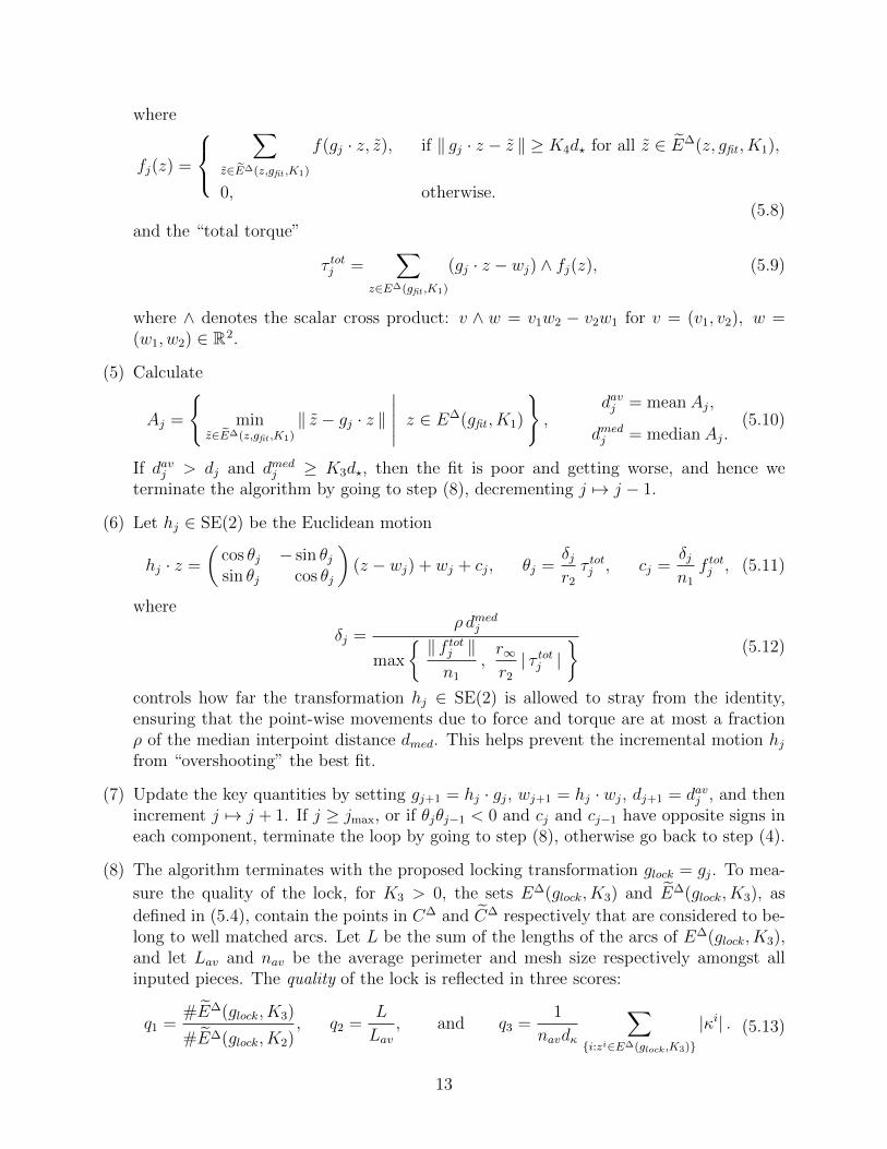
where

fj(z) =

∑

z∈E∆(z,gfit ,K1)

f(gj · z, z), if ‖ gj · z − z ‖ ≥ K4d? for all z ∈ E∆(z, gfit , K1),

0, otherwise.(5.8)

and the “total torque”

τ totj =∑

z∈E∆(gfit ,K1)

(gj · z − wj) ∧ fj(z), (5.9)

where ∧ denotes the scalar cross product: v ∧ w = v1w2 − v2w1 for v = (v1, v2), w =(w1, w2) ∈ R2.

(5) Calculate

Aj =

{min

z∈E∆(z,gfit ,K1)‖ z − gj · z ‖

∣∣∣∣∣ z ∈ E∆(gfit , K1)

},

davj = mean Aj,

dmedj = median Aj.(5.10)

If davj > dj and dmedj ≥ K3d?, then the fit is poor and getting worse, and hence weterminate the algorithm by going to step (8), decrementing j 7→ j − 1.

(6) Let hj ∈ SE(2) be the Euclidean motion

hj · z =

(cos θj − sin θjsin θj cos θj

)(z − wj) + wj + cj, θj =

δjr2

τ totj , cj =δjn1

f totj , (5.11)

where

δj =ρ dmedj

max

{ ‖ f totj ‖n1

,r∞r2

| τ totj |}

(5.12)

controls how far the transformation hj ∈ SE(2) is allowed to stray from the identity,ensuring that the point-wise movements due to force and torque are at most a fractionρ of the median interpoint distance dmed. This helps prevent the incremental motion hjfrom “overshooting” the best fit.

(7) Update the key quantities by setting gj+1 = hj · gj, wj+1 = hj · wj, dj+1 = davj , and thenincrement j 7→ j + 1. If j ≥ jmax, or if θjθj−1 < 0 and cj and cj−1 have opposite signs ineach component, terminate the loop by going to step (8), otherwise go back to step (4).

(8) The algorithm terminates with the proposed locking transformation glock = gj. To mea-

sure the quality of the lock, for K3 > 0, the sets E∆(glock, K3) and E∆(glock, K3), as

defined in (5.4), contain the points in C∆ and C∆ respectively that are considered to be-long to well matched arcs. Let L be the sum of the lengths of the arcs of E∆(glock, K3),and let Lav and nav be the average perimeter and mesh size respectively amongst allinputed pieces. The quality of the lock is reflected in three scores:

q1 =#E∆(glock, K3)

#E∆(glock, K2), q2 =

L

Lav, and q3 =

1

navdκ

∑{i:zi∈E∆(glock,K3)}

|κi| . (5.13)

13

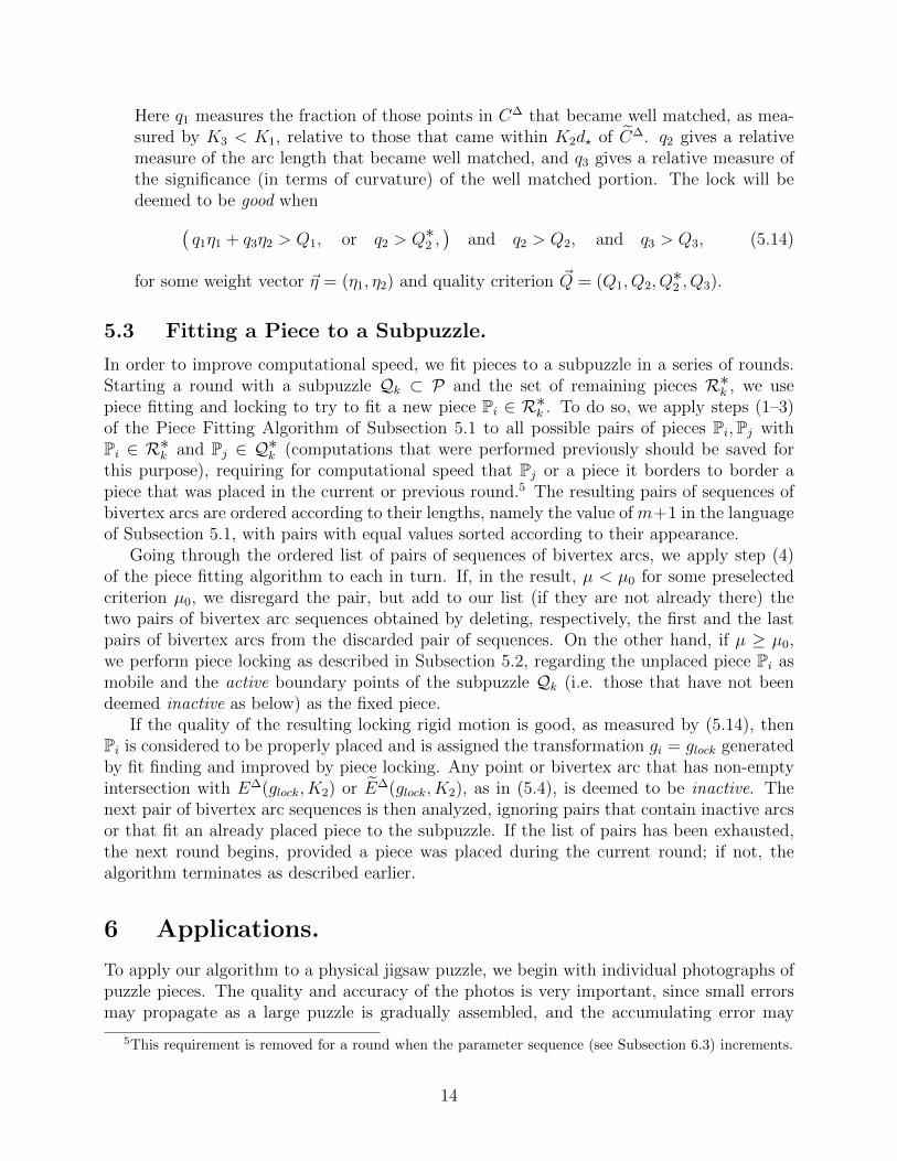
Here q1 measures the fraction of those points in C∆ that became well matched, as mea-sured by K3 < K1, relative to those that came within K2d? of C∆. q2 gives a relativemeasure of the arc length that became well matched, and q3 gives a relative measure ofthe significance (in terms of curvature) of the well matched portion. The lock will bedeemed to be good when(

q1η1 + q3η2 > Q1, or q2 > Q∗2 ,)

and q2 > Q2, and q3 > Q3, (5.14)

for some weight vector ~η = (η1, η2) and quality criterion ~Q = (Q1, Q2, Q∗2 , Q3).

5.3 Fitting a Piece to a Subpuzzle.

In order to improve computational speed, we fit pieces to a subpuzzle in a series of rounds.Starting a round with a subpuzzle Qk ⊂ P and the set of remaining pieces R∗k , we usepiece fitting and locking to try to fit a new piece Pi ∈ R∗k . To do so, we apply steps (1–3)of the Piece Fitting Algorithm of Subsection 5.1 to all possible pairs of pieces Pi,Pj withPi ∈ R∗k and Pj ∈ Q∗k (computations that were performed previously should be saved forthis purpose), requiring for computational speed that Pj or a piece it borders to border apiece that was placed in the current or previous round.5 The resulting pairs of sequences ofbivertex arcs are ordered according to their lengths, namely the value of m+1 in the languageof Subsection 5.1, with pairs with equal values sorted according to their appearance.

Going through the ordered list of pairs of sequences of bivertex arcs, we apply step (4)of the piece fitting algorithm to each in turn. If, in the result, µ < µ0 for some preselectedcriterion µ0, we disregard the pair, but add to our list (if they are not already there) thetwo pairs of bivertex arc sequences obtained by deleting, respectively, the first and the lastpairs of bivertex arcs from the discarded pair of sequences. On the other hand, if µ ≥ µ0,we perform piece locking as described in Subsection 5.2, regarding the unplaced piece Pi asmobile and the active boundary points of the subpuzzle Qk (i.e. those that have not beendeemed inactive as below) as the fixed piece.

If the quality of the resulting locking rigid motion is good, as measured by (5.14), thenPi is considered to be properly placed and is assigned the transformation gi = glock generatedby fit finding and improved by piece locking. Any point or bivertex arc that has non-emptyintersection with E∆(glock, K2) or E∆(glock, K2), as in (5.4), is deemed to be inactive. Thenext pair of bivertex arc sequences is then analyzed, ignoring pairs that contain inactive arcsor that fit an already placed piece to the subpuzzle. If the list of pairs has been exhausted,the next round begins, provided a piece was placed during the current round; if not, thealgorithm terminates as described earlier.

6 Applications.

To apply our algorithm to a physical jigsaw puzzle, we begin with individual photographs ofpuzzle pieces. The quality and accuracy of the photos is very important, since small errorsmay propagate as a large puzzle is gradually assembled, and the accumulating error may

5This requirement is removed for a round when the parameter sequence (see Subsection 6.3) increments.

14

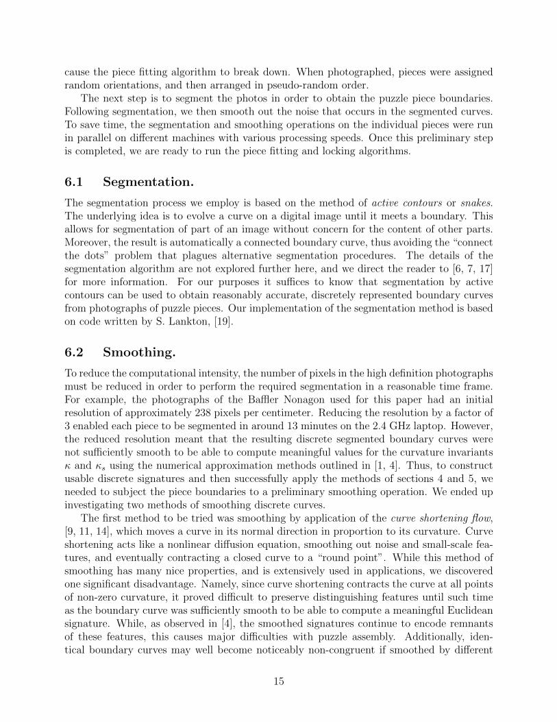
cause the piece fitting algorithm to break down. When photographed, pieces were assignedrandom orientations, and then arranged in pseudo-random order.

The next step is to segment the photos in order to obtain the puzzle piece boundaries.Following segmentation, we then smooth out the noise that occurs in the segmented curves.To save time, the segmentation and smoothing operations on the individual pieces were runin parallel on different machines with various processing speeds. Once this preliminary stepis completed, we are ready to run the piece fitting and locking algorithms.

6.1 Segmentation.

The segmentation process we employ is based on the method of active contours or snakes.The underlying idea is to evolve a curve on a digital image until it meets a boundary. Thisallows for segmentation of part of an image without concern for the content of other parts.Moreover, the result is automatically a connected boundary curve, thus avoiding the “connectthe dots” problem that plagues alternative segmentation procedures. The details of thesegmentation algorithm are not explored further here, and we direct the reader to [6, 7, 17]for more information. For our purposes it suffices to know that segmentation by activecontours can be used to obtain reasonably accurate, discretely represented boundary curvesfrom photographs of puzzle pieces. Our implementation of the segmentation method is basedon code written by S. Lankton, [19].

6.2 Smoothing.

To reduce the computational intensity, the number of pixels in the high definition photographsmust be reduced in order to perform the required segmentation in a reasonable time frame.For example, the photographs of the Baffler Nonagon used for this paper had an initialresolution of approximately 238 pixels per centimeter. Reducing the resolution by a factor of3 enabled each piece to be segmented in around 13 minutes on the 2.4 GHz laptop. However,the reduced resolution meant that the resulting discrete segmented boundary curves werenot sufficiently smooth to be able to compute meaningful values for the curvature invariantsκ and κs using the numerical approximation methods outlined in [1, 4]. Thus, to constructusable discrete signatures and then successfully apply the methods of sections 4 and 5, weneeded to subject the piece boundaries to a preliminary smoothing operation. We ended upinvestigating two methods of smoothing discrete curves.

The first method to be tried was smoothing by application of the curve shortening flow,[9, 11, 14], which moves a curve in its normal direction in proportion to its curvature. Curveshortening acts like a nonlinear diffusion equation, smoothing out noise and small-scale fea-tures, and eventually contracting a closed curve to a “round point”. While this method ofsmoothing has many nice properties, and is extensively used in applications, we discoveredone significant disadvantage. Namely, since curve shortening contracts the curve at all pointsof non-zero curvature, it proved difficult to preserve distinguishing features until such timeas the boundary curve was sufficiently smooth to be able to compute a meaningful Euclideansignature. While, as observed in [4], the smoothed signatures continue to encode remnantsof these features, this causes major difficulties with puzzle assembly. Additionally, iden-tical boundary curves may well become noticeably non-congruent if smoothed by different

15

amounts.To overcome the observed difficulties with curve shortening, we sought a method of

smoothing that led to a meaningful Euclidean signature while still preserving the distin-guishing features. We ended up employing a rather simple spline-based smoothing method.A periodic spline of the points of the curve is calculated. The points are then redistributedevenly by arc-length along the spline in a way that is offset from the original mesh. Wewill refer to this method as the spline-and-respace method of smoothing. In applications,spline-and-respace is carried out a number of times; in our examples 1500 iterations seemedoptimal. We did not try to conduct a rigorous analysis of this method, and we have only em-pirical evidence to support its use. More sophisticated methods based on smoothing splines,e.g., [28], could well be faster and more accurate, but this remains for future investigation.In all of our applications, spline-and-respace smoothing led to a meaningful signature whileretaining all the relevant curve features, and so became our method of choice to smooth thesegmentations of puzzle pieces.

6.3 Generating Solutions.

By applying the segmentation and smoothing algorithms discussed in the preceding subsec-tions, we are able to straightforwardly generate discrete representations of puzzle pieces fromphotographs. We can then apply the puzzle solving algorithm described in section 4. Theperformance of the algorithm depends upon the choice of the following parameters

α, β, γ, C1, C2, p0, m0, µ0, K1, K2, K3, K4, λ0, λ1, ν, ε, ρ, jmax, ~η, ~Q, (6.1)

some of which are introduced in [16]. (The parameter l in that paper only applies to closedcurves, and so does not play a role here.) Of these, p0,m0, and µ0 will be called depthparameters (since for example, decreasing the value of µ0 may increase the number of fits

that are checked by piece locking), while the constants K2, K3, and ~Q will be called qualityparameters since they determine how well pieces must fit to be considered correctly placed.Thus the choice of parameters affects the speed of the algorithm as well as its accuracy.

We observed significant gains in processing speed by allowing the depth parameters tovary during the computation. We search first at a low depth, where correct matches tend tooccur most frequently. But, if the algorithm is unable to place any additional pieces, we thenallow it to search at greater depths. To this end, we introduce a finite sequence of parameters(p0,j,m0,j, µ0,j, K3,j) for 1 ≤ j ≤ j?. The algorithm is first applied with j = 1, but, wheneverit dead-ends, we increment j, terminating the algorithm once j > j?. After a round in whicha piece is successfully placed, we return to j = 1. This allows the algorithm to run at shallowdepths whenever possible and only search deeply in order to get “unstuck.”

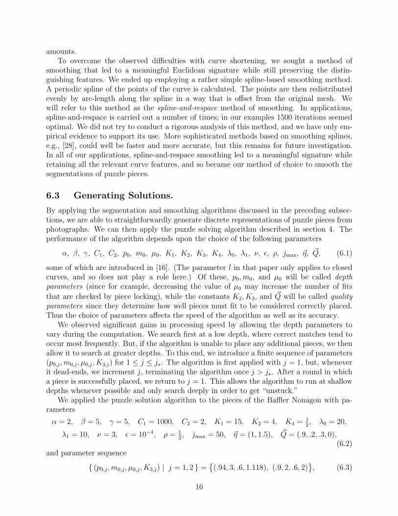
We applied the puzzle solution algorithm to the pieces of the Baffler Nonagon with pa-rameters

α = 2, β = 5, γ = 5, C1 = 1000, C2 = 2, K1 = 15, K2 = 4, K4 = 12, λ0 = 20,

λ1 = 10, ν = 3, ε = 10−4, ρ = 13, jmax = 50, ~η = (1, 1.5), ~Q = (.9, .2, .3, 0),

(6.2)and parameter sequence

{ (p0,j,m0,j, µ0,j, K3,j) | j = 1, 2 } ={

(.94, 3, .6, 1.118), (.9, 2, .6, 2)}, (6.3)

16

so j? = 2. Following segmentation and smoothing, the puzzle was correctly solved in 31minutes. We remark that the solution time should be judged relative to the complexity ofthe pieces. Puzzles that obey the assumptions (1–4) in section 1 allow for simpler solvingalgorithms, which are inherently faster, since the assumptions largely restrict the possiblerelative positions pieces can take (e.g. the rectangular nature of pieces reduces the the numberof (relative) rotations to be checked to the four that align the piece’s straight edges with thoseof the other pieces). Figure 2 displays the pieces as inputed and the solved puzzle.

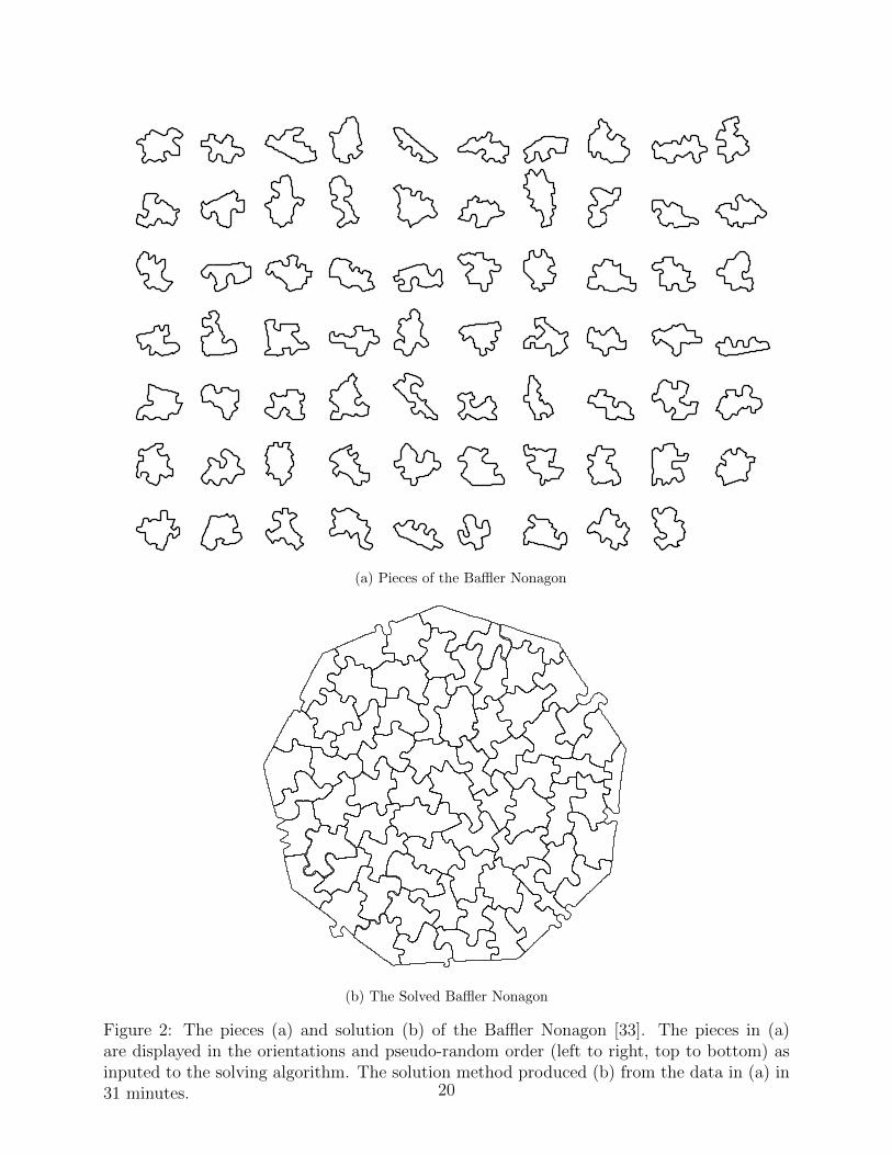
While the unusual shapes of the pieces in the Baffler Nonagon make its solution morechallenging, the fact that they are so different makes errors in piece placement less likely.In order to show that the method is also effective on puzzles with many similar pieces, weapplied it to the simpler (at least to a human) Rain Forest Puzzle [23], with parameters

α = 2, β = 5, γ = 5, C1 = 1000, C2 = 2, K1 = 15, K2 = 4, K4 = 12, λ0 = 30,

λ1 = 10, ν = 3, ε = 10−4, ρ = 13, jmax = 50, ~η = (1, 1.5), ~Q = (.9, .2, .3, 0),

(6.4)and parameter sequence

{ (p0,j,m0,j, µ0,j, K3,j) | j = 1, 2 } ={

(.94, 2, .6, .707), (.9, 2, .6, 2)}. (6.5)

Note that the only difference with the Baffler parameters (6.2), (6.3) is an increase in λ0 anddecrease in m0,1 and K3,1. This is done in order to maintain a better quality control of theprocess, given that the Rain Forest pieces are both significantly larger, and hence of higherresolution, as well as more alike, and so requiring a better quality of fit to ensure properplacement. Following segmentation and smoothing, the puzzle was correctly solved in 58minutes. Figure 3 shows the pieces as inputed and the solved puzzle. Again, we emphasizethat our method makes no a priori assumptions on the shape of the puzzle boundary.

The software used to compute these examples is available for downloading from the secondauthor’s web page: http://math.umn.edu/∼olver/matlab.html

7 Scalability.

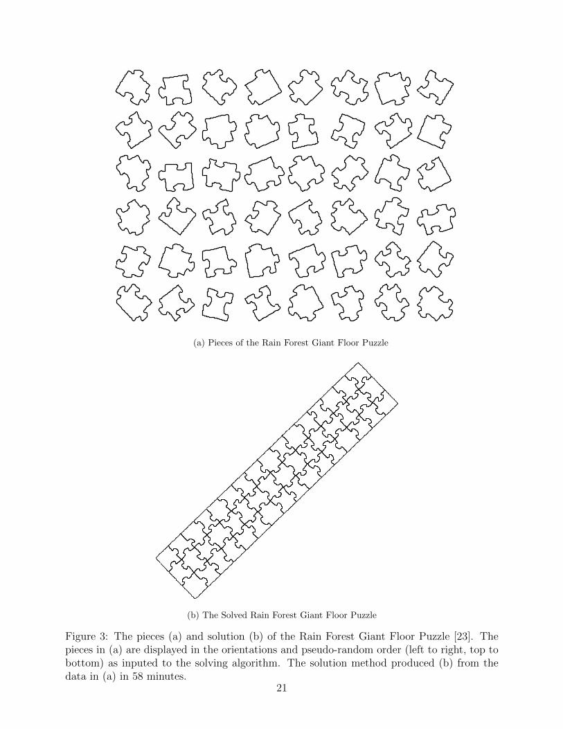
In order to test the scalability of our algorithm, we experimented on portions of the 1000piece Cathedral jigsaw puzzle [29]. This puzzle is non-standard, yet contains many standard“indents” and “outdents.” This combination makes it particularly difficult to solve by com-puter, since there are many “local” near-matches, and yet simplified algorithms cannot beapplied because of the unusual structure.

When addressing larger numbers of puzzles pieces that contained many near-matches, wefound that additional precision is required of the input data. Toward this end, we scannedthe backside of 111 pieces of the Cathedral against a black background on a flatbed scannerat 600 dpi. As above, the images were segmented using active contours. However, in order tominimize the effects of fringes on the pieces, we then applied the following refinement to thesegmentation: First, we fill in (turn to foreground) any patches of background pixels whoseboundary contour is comprised of fewer than 1000 pixels. Then we form the 7-by-7 squarepixel grid centered at each foreground pixel, and change that pixel to background if it lies

17

halfway between any two background pixels in the grid. This step is applied recursively; afterit terminates, the contours are extracted.

Using the resulting data, and parameters

α = 2, β = 5, γ = 5, C1 = 1000, C2 = 2, K1 = 15, K2 = 4, K4 = 12, λ0 = 20,

λ1 = 8, ν = 3, ε = 10−4, ρ = 13, jmax = 50, ~η = (1, 1.5), ~Q = (.976, .24, .3, .029),

(7.1)with (length one) parameter sequence

{ (p0,j,m0,j, µ0,j, K3,j) | j = 1 } ={

(.94, 2, .6, .707)}. (7.2)

the algorithm assembled 103 of the 111 pieces before terminating. Following segmentationand smoothing, the puzzle was solved to this extent in approximately 36 hours. Figure 4shows the pieces as inputed and the partially solved puzzle.

The combination of many near-matches and error in the image processing made high-confidence matching (i.e. the use of high values for Q1, Q2, and Q3) necessary for accuracyin this computation. Hence correct matches may be not be accepted the first time they aretried, but are later once more neighboring pieces have been placed (resulting in higher q1, q2,and q3). This extra care notably increases the computation time, but this effect could bereduced with higher fidelity data. It is also likely that this puzzle fragment would be solvedcompletely if lower values of Q1, Q2 and Q3 were employed after the algorithm “dead-ends”as part of a modified parameter sequence.

Another factor that entered into play with the larger puzzle was accumulation of errors. Inparticular, we noted some differences in long-term performance on machines running differentoperating systems. Although at this time we have not explored it fully, we believe this islargely due to the repeated composition of Euclidean transformations stored in different forms(compare (2.1) and (5.11)) using sine and cosine functions compiled to varying accuracies.

8 Further Directions.

Our results indicate a number of different directions that are worth pursuing. The first areconcerned with improving the puzzle solving algorithms as developed so far. One immediateissue worth further investigation is the specification of the various parameters (6.1). Whilesome work was already done in this direction, particularly our realization that the depthparameters could be profitably adjusted during the course of the assembly algorithms, wedid not conduct a systematic investigation into fine tuning the parameter values for optimalperformance, which may well depend upon the nature of the puzzle, the accuracy of thephotographs of the pieces and their segmented/smoothed boundaries, and the desired speedof computation. A future research project will be to better understand the optimal parametervalues, perhaps through automatic learning on a larger training set. It would be interestingto see our program compete with human puzzle solvers, particularly in challenging cases likethe Baffler Nonagon, or puzzles that allow overlapping pieces, if such can be devised.

We were pleasantly surprised by the algorithm’s ability to accurately place pieces, andthen completely solve the challenging large-scale puzzles we tried it on. We had initiallyexpected to require it to do a fair amount of backtracking in the event that a piece is

18

wrongly placed, and allowed for that possibility to be incorporated in our code. If morechallenging examples require revisiting this part of the algorithm, a careful analysis of therelevant backtracking and branching rules would be worth doing. This would be particularlyuseful for dealing with puzzles whose pieces fit together in multiple ways, not all of whichare compatible with the final assembly. We had also envisioned having to readjust the earlierpiece placements if their accumulated errors prevented completing the puzzle, even whencorrectly placed. One idea, motivated by the numerical algorithm of simulated annealing,[21], would be to employ random perturbations to “jiggle” all the pieces in a subpuzzle inorder to improve its overall fit quality.

Provided the photographs of the individual pieces are sufficiently accurate, the segmenta-tion algorithm does a fine job of locating a decent approximation to their boundaries. On theother hand, the simple spline-and-respace smoothing method could certainly be improved,perhaps by using the more sophisticated approaches developed in [28]. Spline smoothingmight also be enhanced by linking it to the approximate bivertex decomposition of the pieceboundaries, e.g., by respacing the nodes in a non-uniform manner. For instance, we foundthat weighting the mesh density by κs gives some intriguing results, but this requires furtherinvestigation before being useful.

One question that might occur to the reader is why use two steps to place the pieces: piecefitting based on the bivertex arcs followed by piece locking. We did contemplate bypassingthe signature matching step, and using piece-locking alone, but the latter algorithm is muchslower than signature comparison, and hence, as it stands, would not produce the desiredmatching results as efficiently. Moreover, in order to characterize the bivertex arcs, we haveeffectively already computed their signatures, and so by this stage signature matching isextremely efficient.

It would certainly be worthwhile extending our algorithms, both for fitting and smoothing,to be more attuned to corners, but this was not pursued as it turned out to be unnecessaryto successfully solve the puzzles we considered. Furthermore, developing a way to universallytreat subpuzzles as single pieces, while unnecessary in the examples treated here, couldmake the algorithm more robust. Building on this, a more sophisticated approach wouldbe to allow several distinct subpuzzles to be assembled concurrently, and then deal withthe problem of fitting them together. Finally, methods that incorporate overall designs orpictures on the puzzle with our shape matching algorithms will be left to future research.In a practical direction, it would be very revealing to test our algorithms on other typesof assembly problems, such as broken archaeological artifacts, e.g., ceramics or pottery, orshredded documents.

Since our extended signature methods are semi-local, based on subarcs of boundary curves,they could also be readily adapted to the problems of recognizing and reconstructing objectsunder partial occlusion, [2, 27]. Indeed, our piece locking refinement could be applied back tothe original problem of object recognition, [4, 16], with or without occlusion, to, we expect,great effect. Finally, in a more speculative vein, one might try to extend these methods tosolving fully three-dimensional puzzles, e.g., broken statues. The underlying Cartan equiv-alence method applies to general submanifolds, and the corresponding differential invariantsignatures that uniquely characterize (sufficiently regular) surfaces under rigid motions areknown, [20]. However, there are major practical, numerical, and computational issues thatneed resolving before such an extension can be contemplated.

19

(a) Pieces of the Baffler Nonagon

(b) The Solved Baffler Nonagon

Figure 2: The pieces (a) and solution (b) of the Baffler Nonagon [33]. The pieces in (a)are displayed in the orientations and pseudo-random order (left to right, top to bottom) asinputed to the solving algorithm. The solution method produced (b) from the data in (a) in31 minutes. 20

(a) Pieces of the Rain Forest Giant Floor Puzzle

(b) The Solved Rain Forest Giant Floor Puzzle

Figure 3: The pieces (a) and solution (b) of the Rain Forest Giant Floor Puzzle [23]. Thepieces in (a) are displayed in the orientations and pseudo-random order (left to right, top tobottom) as inputed to the solving algorithm. The solution method produced (b) from thedata in (a) in 58 minutes.

21

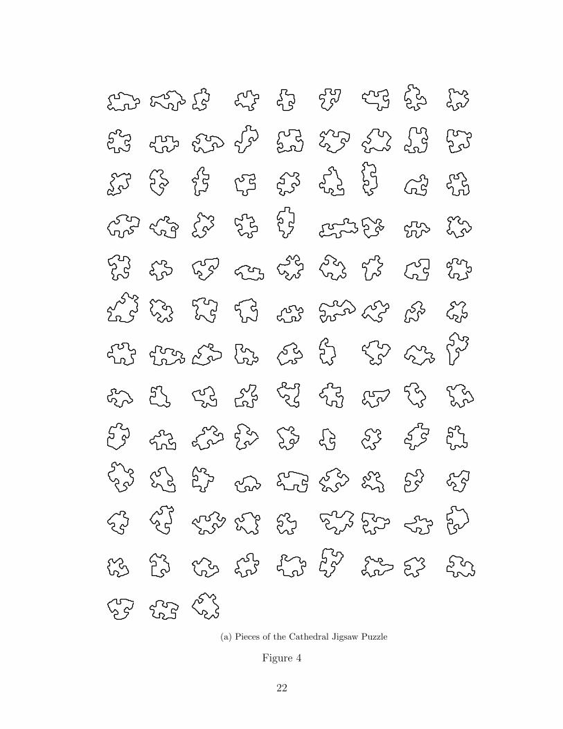
(a) Pieces of the Cathedral Jigsaw Puzzle

Figure 4

22

(b) Partial Solution to the Cathedral Jigsaw Puzzle

Figure 4: The pieces (a) and 103 piece partial solution (b) of the Cathedral Jigsaw Puzzle[29]. The pieces in (a) are displayed in the orientations and pseudo-random order (left toright, top to bottom) as inputed to the solving algorithm. The solution method produced(b) from the data in (a) in approximately 36 hours. We note that (b) has been rotated 90degrees clockwise from the output in order to better fit the page.

23

References

[1] Boutin, M., Numerically invariant signature curves, Int. J. Computer Vision 40 (2000),235–248.

[2] Bruckstein, A.M., Holt, R.J., Netravali, A.N., and Richardson, T.J., Invariant signaturesfor planar shape recognition under partial occlusion, CVGIP: Image Understanding 58(1993), 49–65.

[3] Burdea, G.C., and Wolfson, H.J., Solving jigsaw puzzles by a robot, IEEE Transactionson Robotics and Automation 5 (1989), 752–764.

[4] Calabi, E., Olver, P.J., Shakiban, C., Tannenbaum, A., and Haker, S., Differential andnumerically invariant signature curves applied to object recognition, Int. J. ComputerVision 26 (1998), 107–135.

[5] Cartan, E., Les problemes d’equivalence, in: Oeuvres Completes, part. II, vol. 2,Gauthier–Villars, Paris, 1953, pp. 1311–1334.

[6] Caselles, V., Kimmel, R., and Sapiro, G., Geodesic active contours, Int. J. ComputerVision 22 (1997), 61–79.

[7] Chan, T., and Vese, L., Active contours without edges, IEEE Transactions on ImageProcessing 10 (2001), 266–277.

[8] The DARPA Shredder Challenge, http://www.shredderchallenge.com/, 2011.

[9] Deckelnick, K., Dziuk, G., and Elliott, C.M., Computation of geometric partial differ-ential equations and mean curvature flow, Acta Numer. 14 (2005), 139–232.

[10] Freeman, H., and Carder, L., Apictorial jigsaw puzzles: the computer solution of aproblem in pattern recognition, IEEE Trans. Elec. Comp. 13 (1964), 118–127.

[11] Gage, M., and Hamilton, R.S., The heat equation shrinking convex plane curves, J. Diff.Geom. 23 (1986), 69–96.

[12] Gallagher, A.C., Jigsaw puzzles with pieces of unknown orientation, in: 2012 IEEEConference on Computer Vision and Pattern Recognition (CVPR), IEEE Comp. Soc.Press, Los Alamitos, CA, 2012, pp. 382–389.

[13] Goldberg, D., Malon, C., and Bern, M., A global approach to the automatic solution ofjigsaw puzzles, Computational Geometry 28 (2004), 165–174.

[14] Grayson, M., The heat equation shrinks embedded plane curves to round points, J. Diff.Geom. 26 (1987), 285–314.

[15] Guggenheimer, H.W., Differential Geometry, McGraw–Hill, New York, 1963.

[16] Hoff, D., and Olver, P.J., Extensions of invariant signatures for object recognition, J.Math. Imaging Vision 45 (2013), 176–185.

24

[17] Kichenassamy, S., Kumar, A., Olver, P.J., Tannenbaum, A., and Yezzi, A., Conformalcurvature flows: from phase transitions to active vision, Arch. Rat. Mech. Anal. 134(1996), 275–301.

[18] Kong, W., and Kimia, B.B., On solving 2D and 3D puzzles using curve matching,Proceedings of the 2001 IEEE Computer Society Conference on Computer Vision andPattern Recognition 2 (2001), 583–590.

[19] Lankton, S., Active Contours, http://www.shawnlankton.com/2007/05/active

-contours/, 2007.

[20] Olver, P.J., Equivalence, Invariants, and Symmetry, Cambridge University Press, Cam-bridge, 1995.

[21] Pham, D.T., and Karaboga, D., Intelligent Optimisation Techniques : Genetic Algo-rithms, Tabu Search, Simulated Annealing and Neural Networks, Springer–Verlag, NewYork, 2000.

[22] Radack, G.M., and Badler, N.I., Jigsaw puzzle matching using a boundary-centeredpolar encoding, Comp. Graphics Image Proc. 19 (1982), 1–17.

[23] The Rain Forest Giant Floor Puzzle, Frank Schaffer Publications, Inc., Torrance, CA,1992.

[24] Sagiroglu, M.S., and Ercil, A., A texture based approach to reconstruction of archaeo-logical finds, in: Proceedings of the 6th International conference on Virtual Reality, Ar-chaeology and Intelligent Cultural Heritage, VAST05, Mudge, M., Ryan, N., Scopigno,R., eds., Eurographics Assoc., Aire-la-Ville, Switzerland, 2005, pp. 137–142.

[25] Shakiban, C., and Lloyd, P., Signature curves statistics of DNA supercoils, in: Geometry,Integrability and Quantization, vol. 5, I.M. Mladenov and A.C. Hirschfeld, eds., Softex,Sofia, Bulgaria, 2004, pp. 203–210.

[26] Shakiban, C., and Lloyd, R., Classification of signature curves using latent semantic anal-ysis, in: Computer Algebra and Geometric Algebra with Applications, H. Li, P.J. Olver,and G. Sommer, eds., Lecture Notes in Computer Science, vol. 3519, Springer–Verlag,New York, 2005, pp. 152–162.

[27] Turney, J.L., Mudge, T.N., and Volz, R.A., Recognizing partially occluded parts, IEEETrans. Pattern Anal. Machine Intel. 7 (1985), 410–421.

[28] Wang, Y., Smoothing Splines : Methods and Applications, Monographs Stat. Appl. Prob-ability, vol. 121, CRC Press, Boca Raton, FL, 2011.

[29] Wesley, R., Cathedral, Product #51015, SunsOut, Inc., Costa Mesa, CA.

[30] Wolfson, H., Schonberg, E., Kalvin, A., and Lamdan, Y., Solving jigsaw puzzles bycomputer, Annals of Operations Research 12 (1988), 51–64.

25

[31] Wu, K., and Levine, M.D., 3D part segmentation using simulated electrical charge dis-tributions, IEEE Trans. Pattern Anal. Machine Intel. 19 (1997), 1223–1235.

[32] Feng-Hui Yao, F.–H., and Shao, G.–F., A shape and image merging technique to solvejigsaw puzzles, Pattern Recognition Lett. 24 (2003), 1819–1835.

[33] Yates, C., The Baffler: the nonagon, Ceaco, Newton, MA, 2010.

[34] Zisserman, A., Forsyth, D.A., Mundy, J.L., and Rothwell, C.A., Recognizing generalcurved objects efficiently, in: Geometric Invariance in Computer Vision, J.L. Mundyand A. Zisserman, eds., MIT Press, Cambridge, Mass., 1992, pp. 228–251.

26