Automatic Segmentation of Menisci in MR

Images Using Pattern Recognition and Graph

Cuts

Fredrik Nedmark, fredrik_n84@hotmail.com

April 14, 2011

Abstract

In this Master’s thesis a system for automatic segmentation of the menisci inmagnetic resonance (MR) images is developed and tested. MR imaging is anon invasive method with no ionization and with good soft tissue contrast andconstitutes an important tool to evaluate soft tissue, tendon, ligaments andmenisci in the knee. The menisci are located between the femur (thigh bone)and patella (shin bone) in the knee and has several functions, such as shockabsorption. Medical imaging systems have been improved during the last decades.Images today are produced with higher resolution and faster acquisition timethan before. Processing these images manually is very time consuming. Thereforeit is necessary to create computerized tools that can be used by the medical staffin their work with diagnosis of illness and treatments of patients. The approachfor constructing the automatically segment system is divided into three subparts.The first task is to extract all bone parts from the images. Secondly, the areawhere the menisci can be found is localized and the final step is to segmentthe menisci. This thesis is mainly based on two methods and they are patternrecognition with Laws’ texture features and Graph Cut. In this thesis the systemis tested on five examinations produced in Landskrona hospital from a Philips1.5T machine using a spin-echo sequence. The result is promising and couldwith further work become an accurate system for automatically segmenting themenisci.

Acknowledgements

I would like to thank Magnus Tagil at the Department of Orthopedics in Lundfor valuable comments, support and test materials. I would also like to thanks mysupervisors Kalle Astrom and Petter Strandmark at the Mathematical ImagingGroup at the Centre for Mathematical Sciences in Lund for their guidance,helpful comments and support.

Contents

1 Magnetic Resonance Images of the Knee 21.1 What is the Meniscus? . . . . . . . . . . . . . . . . . . . . . . . . 31.2 Magnetic Resonance Imaging (MRI) . . . . . . . . . . . . . . . . 31.3 Image Acquisition . . . . . . . . . . . . . . . . . . . . . . . . . . 61.4 Related Work . . . . . . . . . . . . . . . . . . . . . . . . . . . . . 7

2 Theory 92.1 Laws’ Texture Algorithm . . . . . . . . . . . . . . . . . . . . . . 92.2 Graph Cut . . . . . . . . . . . . . . . . . . . . . . . . . . . . . . 11

3 Segmentation Workflow 153.1 Segmentation of Bone . . . . . . . . . . . . . . . . . . . . . . . . 15

3.1.1 Create Classdata with Laws’ Texture Algorithm . . . . . 183.1.2 Segmentation Process for Segmenting Bone With Graph Cut 18

3.2 Find the Correct Localization of the Menisci . . . . . . . . . . . 223.3 Segmentation of the Menisci . . . . . . . . . . . . . . . . . . . . . 22

3.3.1 Finding the Mean Intensities of the Meniscus . . . . . . . 233.3.2 Segmentation Process . . . . . . . . . . . . . . . . . . . . 25

4 Results 324.1 Result of Bone Segmentation . . . . . . . . . . . . . . . . . . . . 324.2 Result from Locating the Menisci Locations . . . . . . . . . . . . 334.3 Segmentation Result of the Menisci . . . . . . . . . . . . . . . . . 344.4 Evaluation of the Results from the Automatic Segmentation . . . 38

4.4.1 Examination 1 . . . . . . . . . . . . . . . . . . . . . . . . 394.4.2 Examination 2 . . . . . . . . . . . . . . . . . . . . . . . . 394.4.3 Examination 4 . . . . . . . . . . . . . . . . . . . . . . . . 394.4.4 Examination 5 . . . . . . . . . . . . . . . . . . . . . . . . 394.4.5 Examination 5 again . . . . . . . . . . . . . . . . . . . . . 404.4.6 Summary . . . . . . . . . . . . . . . . . . . . . . . . . . . 40

5 Future work 45

1

Chapter 1

Magnetic Resonance Imagesof the Knee

During the last several decades medical imaging systems have improved consid-erably. The systems have improved both in terms of better resolution and fasteracquisition speed. Images have become a necessary part of todays patient caresince they are used in diagnosis and treatment of patients. This is the reasonwhy the number of produced images increases and why it is important to createcomputerized tools for their analysis. Computerized tools extract informationthat hopefully will help the medical staff with faster and more accurate analysis,cf. [7, page 1].

The aim of this Master’s thesis is to automatically segment the menisci from aMagnetic Resonance Imaging (MRI) examination. MRI is a non invasive methodwith no ionization and with good soft tissue contrast, cf. [7, page 18]. ThisMaster’s thesis was made in collaboration with Magnus Tagil at the Departmentof Orthopedics in Lund and the Mathematical Imaging Group at the Centrefor Mathematical Sciences in Lund. The MR images that were used during thiswork were produced at the hospital in Landskrona. The approach during thisthesis is mainly divided into three subparts. The first task is to extract all boneparts from the images. Secondly, the area where the menisci can be found islocalized and the final step is to segment the menisci. Two main methods areused in this thesis: pattern recognition with Laws’ texture features and GraphCut.

The content of this thesis can be summarized as followed: Chapter 1 containsessential background information that is needed to understand the work thathas been done. Chapter 2 covers the theory of different methods used in thework. Chapter 3 contains a description of the workflow of the program. Chapter4 includes a discussion of the results. In chapter 5 future work is discussed.

2

1.1 What is the Meniscus?

The basic anatomy of the human knee bone parts is shown in figure 1.1. Inthese images the major bone parts are visible from different angles. The leftimage shows the frontal view also known as the coronal plane, see figure 1.2 formore information about the discussed body planes. The right image shows thesagittal view of the knee. Bone parts of interest are the femur, tibia and patella.The meniscus shape is well known and looks like a crescent shaped object offibrocartilage that is located between the surfaces of the femur and tibia, seefigure 1.3. In a normal human knee two menisci can be found, one lateral andone medial. The name reflect the location where the menisci can be found. Thelateral meniscus is located on the outside of the knee and the medial on theinside. This is visible in figure 1.3 and 1.4. Figure 1.4 shows the meniscus fromthe transverse plane. From this figure both menisci are visible from above. Infigure 1.3 the knee is shown in the frontal plane and the location of the meniscusis pointed out with an arrow. Also observe the meniscus horns that has beenpointed out in figure 1.3 but is still fully visible in figure 1.4. The meniscushorns plays a major part in this thesis. In the sagittal view the horns have acharacteristic triangular shape, which can be used when trying to locate themeniscus.

The meniscus plays an important role for biomechanical functions. Aspreviously stated, it is located between the femur and tibia, therefore oneessential purpose is to act as load bearer and shock absorber. This is also thereason for why the loss of meniscus increases the risk of developing osteoarthritisin the knee since the forces are distributed on a smaller area. Other importanttasks are helping stabilizing the knee joint and lubrication of the joint surfaces,cf. [15, 6].

1.2 Magnetic Resonance Imaging (MRI)

MRI is a non invasive technique with no ionizing radiation that creates highquality images of the inside of the human body. To create images of the structuresinside the body the nuclear spin of the hydrogen atoms are used. By adding astrong external static magnetic field, about 1-10 T, the majority of the hydrogenatoms have their spin pointing in the same direction creating the magnetizationvector which precess around the static magnetic field at the resonance frequency.An external electromagnetic radio frequency (RF) pulse at the resonant frequencyis transmitted. The RF pulse will flip the magnetization vector into the planeperpendicular to the static magnetic field where the signal can be detected.

Echo time, Te, is the time between the RF pulse and the time when thesignal is detected. For more detailed information regarding how the MR workssee [7]. There are mainly two important properties. First of all the protondensity and secondly the two relaxation times called spin-lattice and spin-spinrelaxation time are of interest. These relaxation times are also called T1 andT2 respectively. The relaxation time is a measure of how long time it takes for

3

Figure 1.1: The figure illustrates the basic bone anatomy of the human knee asseen from the coronal plane (left) and from the sagittal plane (right).Observe the major bone parts femur, tibia, fibula and patella thatalso are visible in MR images of the knee. Image credit: Strover S,http://www.kneeguru.co.uk.

Figure 1.2: The figure shows the three reference planes from were the MRI slices aretaken from. The directions are the sagittal, coronal and the transverse.

4

Figure 1.3: The figure illustrates the location of the menisci. The knee is shownfrom the frontal view and the meniscus is located at the contact surfacesbetween the femur and tibia. Note that each knee has two menisci,known as the lateral and medial meniscus. Image credit: Strover S,http://www.kneeguru.co.uk.

Figure 1.4: The figure shows the basic parts of the meniscus from above. Note theendpoints of the half moon shaped meniscus, on both the lateral andmedial meniscus, refereed to as the posterior and anterior horns. Imagecredit: Strover S, http://www.kneeguru.co.uk.

5

Figure 1.5: The figure illustrates how the signal depends on the tissue. The image tothe left shows the signal behavior from a T1-weighted examination andthe right a T2-weighted examination. Since the signal depends on thetissue the diffrent tissue types will have different intensities in the MRimage. Image credit: e-MRI, Hoa D, www.imaios.com.

the tissue to get back to equilibrium after the RF-signal and this depends ondifferent tissue types. T1-weighted images give a weak signal for long T1 timesand T2-weighted give a high signal for long T2 time, cf. [7, page 31-32], seefigure 1.5. The difference in the signal strength creates an intensity differencebetween the different tissues in a MR image.

As previously indicated one important property is the proton density andthat makes MR sensitive to water which makes up to 70-90% of most tissue. Theamount of water in the tissue can alter with diseases or injury which changes theoutput signal compared to a healthy tissue, cf. [22, page 4]. This makes MRIan excellent tool to evaluate soft tissue, tendon, ligaments and menisci in theknee, cf. [22, page 24]. In MR, several 2D slices are produced to create a 3Dobject that can be visualized. In figure 1.2 the body plane with the three majordirections are shown. The directions are the sagittal, coronal and transverseplane.

1.3 Image Acquisition

Images used in this Masters’s thesis were produced at the hospital in Landskronafrom a Philips 1, 5T machine using a spin-echo sequence with repetition time2 s, echo time 8.8 ms, matrix size 512× 512 pixels, pixel spacing 0.28× 0.28 mmand slice thickness 3 mm.

6

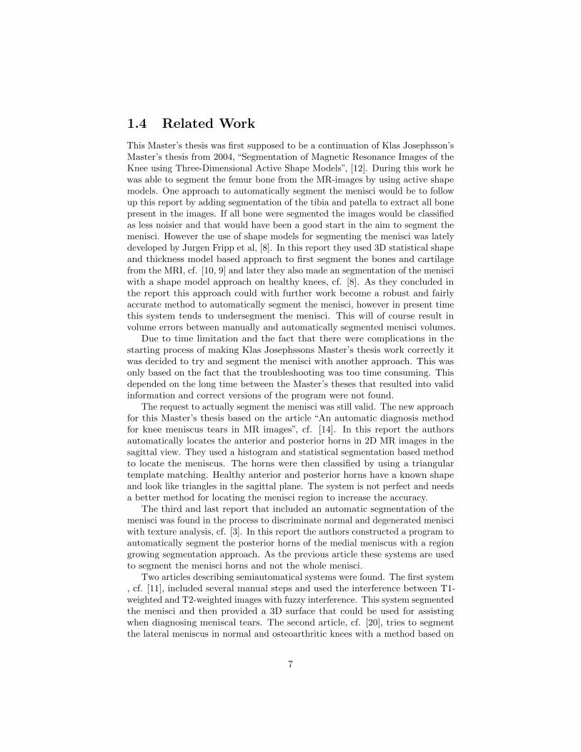
1.4 Related Work

This Master’s thesis was first supposed to be a continuation of Klas Josephsson’sMaster’s thesis from 2004, “Segmentation of Magnetic Resonance Images of theKnee using Three-Dimensional Active Shape Models”, [12]. During this work hewas able to segment the femur bone from the MR-images by using active shapemodels. One approach to automatically segment the menisci would be to followup this report by adding segmentation of the tibia and patella to extract all bonepresent in the images. If all bone were segmented the images would be classifiedas less noisier and that would have been a good start in the aim to segment themenisci. However the use of shape models for segmenting the menisci was latelydeveloped by Jurgen Fripp et al, [8]. In this report they used 3D statistical shapeand thickness model based approach to first segment the bones and cartilagefrom the MRI, cf. [10, 9] and later they also made an segmentation of the menisciwith a shape model approach on healthy knees, cf. [8]. As they concluded inthe report this approach could with further work become a robust and fairlyaccurate method to automatically segment the menisci, however in present timethis system tends to undersegment the menisci. This will of course result involume errors between manually and automatically segmented menisci volumes.

Due to time limitation and the fact that there were complications in thestarting process of making Klas Josephssons Master’s thesis work correctly itwas decided to try and segment the menisci with another approach. This wasonly based on the fact that the troubleshooting was too time consuming. Thisdepended on the long time between the Master’s theses that resulted into validinformation and correct versions of the program were not found.

The request to actually segment the menisci was still valid. The new approachfor this Master’s thesis based on the article “An automatic diagnosis methodfor knee meniscus tears in MR images”, cf. [14]. In this report the authorsautomatically locates the anterior and posterior horns in 2D MR images in thesagittal view. They used a histogram and statistical segmentation based methodto locate the meniscus. The horns were then classified by using a triangulartemplate matching. Healthy anterior and posterior horns have a known shapeand look like triangles in the sagittal plane. The system is not perfect and needsa better method for locating the menisci region to increase the accuracy.

The third and last report that included an automatic segmentation of themenisci was found in the process to discriminate normal and degenerated menisciwith texture analysis, cf. [3]. In this report the authors constructed a program toautomatically segment the posterior horns of the medial meniscus with a regiongrowing segmentation approach. As the previous article these systems are usedto segment the menisci horns and not the whole menisci.

Two articles describing semiautomatical systems were found. The first system, cf. [11], included several manual steps and used the interference between T1-weighted and T2-weighted images with fuzzy interference. This system segmentedthe menisci and then provided a 3D surface that could be used for assistingwhen diagnosing meniscal tears. The second article, cf. [20], tries to segmentthe lateral meniscus in normal and osteoarthritic knees with a method based on

7

thresholding and morphological operations. This system needs some manuallysteps and the segmentation result is not always that accurate.

8

Chapter 2

Theory

2.1 Laws’ Texture Algorithm

Texture analysis is used in several areas such as classification and segmentationproblems. Textures are various patterns in images. Identifying these patternsis a result of extracting features from patterns in different images. In 1979 K.ILaws proposed a texture energy approach, cf. [19], that classifies each pixel byextracting features. The method estimates the energy inside a region of interestby energy transformation. The transformation only requires convolution and amoving window technique. Laws’ developed a two-dimensional set of filter masksthat was derived from five one-dimensional filters. The set is used to detectfeatures from patterns. Each one-dimensional filter vector was constructed todetect different microstructure in the images. Microstructure of interest are leveldetection, edge detection, spot detection, wave detection and ripple detection, cf.[18, 16, 17, 19].

Level detection: L5 = [1 4 6 4 1].Edge detection: E5 = [-1 -2 0 2 1].Spot detection: S5 = [-1 0 2 0 -1].Ripple detection: R5 = [1 -4 6 -4 1].Wave detection: W5 = [-1 2 0 -2 -1].

From these one dimensional vectors 25 two-dimensional masks m of size 5×5were created by convolution between all possible combinations of these vectorsand their transpose. 24 of these masks are zero-sum but the mL5L5

is not. Theresult is referred to as ml, where l indicates which of these masks that is used,

LT5 L5 LT

5 E5 LT5 S5 LT

5 R5 LT5 W5

ET5 L5 ET

5 E5 ET5 S5 ET

5 R5 ET5 W5

ST5 L5 ST

5 E5 ST5 S5 ST

5 R5 ST5 W5

RT5 L5 RT

5 E5 RT5 S5 RT

5 R5 RT5 W5

WT5 L5 WT

5 E5 WT5 S5 WT

5 R5 WT5 W5

9

The approach to extract features with Laws’ texture algorithm in this Master’sthesis is divided into three parts:

1: Construct the different masks.

2: Construct energy measurement.

3: Calculate features from energy measurements.

First the image I(i, j) of size r× c needs some preprocessing before it is readyto be analyzed. Images to be analyzed with Laws’ texture in this thesis all havethe same size of 5× 5 pixels. The purpose of the preprocessing is to erase themean intensity of the image and keep the interesting parts of the image,

f = I −∑r

i=1

∑cj=1 I(i, j)

r · c. (2.1)

This will give a better picture of how the environment or in this case the texturesrandomness looks like. This new image will be convoluted with each of themasks,

TIl = f ∗ml. (2.2)

Each texture image, TIl, will be normalized with the L5L5 mask since this maskhad not zero mean as discussed earlier. The texture energy measurements, TEM ,will be calculated by moving a window in the normalized images. The windowsummarizes the absolute value in a neighborhood of 5× 5 pixels. This will createa new set of 25 images of size 5× 5 pixels known as TEM. Note that the imagesize of the TIl was 9× 9 pixels i.e. the image sizes are back to the original sizesafter this texture energy measurement,

TEMl(i, j) =

i+2∑m=i−2

j+2∑n=j−2

|TIl(m,n)| . (2.3)

By combining similar features with each other a set of 14 new images is created,

TRX5Y 5 =TEMX5Y 5 + TEMY 5X5

2, (2.4)

where X5Y5 indicates which of the masks that is added to each other. Forinstance a single image that is sensitive to edges, TRE5L5

, is created by addingthe TEME5L5

with the TEML5E5, where TEME5L5

is sensitive to the horizontaledges and the TEML5E5

is sensitive to the vertical edges.The final 14 images are,

TRE5E5TRE5L5

TRE5S5TRE5R5

TRE5W5

TRL5S5 TRL5R5 TRL5W5 TRS5S5 TRS5R5

TRS5W5 TRR5R5 TRR5W5 TRW5W5 .

Features used in this thesis are extracted from these 14 images. From eachimage five features are calculated. The features are mean intensity, standarddeviation, entropy, skewness and kurtosis. One additional feature is added andthat is the mean intensity from the original image. This implies that 71 featuresare calculated to each image that is being analyzed .

10

2.2 Graph Cut

Graph cuts is a well known method for image segmentation. The image isoptimally divided into two parts by calculating the min-cut between the segmentsknown as the foreground and background.

A graph G(V,E) consists of a collection of nodes, or vertices (V ), and acollection of edges (E) that connect the vertices with nonnegative weights we.In an image all pixels will be represented as a vertex and the edges are thelinks between the neighboring pixels. Two additional vertices are connectedto each pixel, also known as the terminal nodes and they represent the fore-ground/background labeling. The first terminal node is refereed to as source,s, and represents the foreground. The other terminal is known as sink, t, andrepresents the background. Edges are often divided in two parts. The first part,n-links, connects pairs of neighboring vertices. An edge connects two verticesand the cost will be weighted depending on the similarity between the pixel andits surrounding. In 2D the neighborhood consists of the 4 or 8 closest vertices.The second part, t-link, connects the vertices with the terminals. This meansthat the cost between the vertex and the terminal corresponds to the penaltyfor assigning the vertex to that specific terminal.

The image in the left column in figure 2.1 illustrates an image of 3× 3 pixels.As said before each vertex is connected to the terminal nodes s and t as seen inthe image in the middle column, t-link. The image in the right column showshow the pixels are connected to each other, n-link. In this example the pixelsare connected to the four closest pixels.A cut is to separate the vertices in two disjoint subsets, S and T, so that nopaths from the terminal nodes s and t exist to each other. In other words s ∈ S,t ∈ T , S ⊂ V and T ⊂ V . The cut can be performed in many ways, howeverthere will always be a cut that have the minimum cost, i.e. min-cut. Figure 2.2illustrates a cut in the image of 3× 3 pixels where the subset connected to thesource (s) is called the foreground and the subset connected to the sink(t) iscalled the background.

In this Master’s thesis the implementation of graph cut algorithm by Boykovand Kolmogorov is used to calculate the min-cut or max-flow [5]. This min-cut/max flow can be calculated by minimizing the discrete approximation to theenergy function,

E(γ) = λ length(γ)︸ ︷︷ ︸regularization term

+

∫∫Γ

(I(x)− µ1)2 dx +

∫∫Ω/Γ

(I(x)− µ0)2 dx︸ ︷︷ ︸data terms

, (2.5)

where I is the image and the foreground and background are modeled as havinga constant intensity, µ0 and µ1 respectively. The segmentation problem involvesfinding a curve γ that minimizes the energy E(γ) so that the region inside Γ islabeled as foreground and the remaining parts are labeled as background, see

11

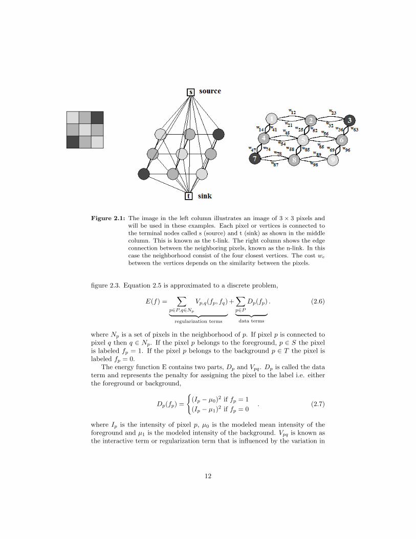
Figure 2.1: The image in the left column illustrates an image of 3 × 3 pixels andwill be used in these examples. Each pixel or vertices is connected tothe terminal nodes called s (source) and t (sink) as shown in the middlecolumn. This is known as the t-link. The right column shows the edgeconnection between the neighboring pixels, known as the n-link. In thiscase the neighborhood consist of the four closest vertices. The cost we

between the vertices depends on the similarity between the pixels.

figure 2.3. Equation 2.5 is approximated to a discrete problem,

E(f) =∑

p∈P,q∈Np

Vp,q(fp, fq)

︸ ︷︷ ︸regularization terms

+∑p∈P

Dp(fp)︸ ︷︷ ︸data terms

. (2.6)

where Np is a set of pixels in the neighborhood of p. If pixel p is connected topixel q then q ∈ Np. If the pixel p belongs to the foreground, p ∈ S the pixelis labeled fp = 1. If the pixel p belongs to the background p ∈ T the pixel islabeled fp = 0.

The energy function E contains two parts, Dp and Vpq. Dp is called the dataterm and represents the penalty for assigning the pixel to the label i.e. eitherthe foreground or background,

Dp(fp) =

(Ip − µ0)2 if fp = 1

(Ip − µ1)2 if fp = 0. (2.7)

where Ip is the intensity of pixel p, µ0 is the modeled mean intensity of theforeground and µ1 is the modeled intensity of the background. Vpq is known asthe interactive term or regularization term that is influenced by the variation in

12

Figure 2.2: A cut is to separate the vertices in two disjoint subsets, S and T, so thatno paths from the terminal nodes s and t exist.

Figure 2.3: This figure illustrates a segmented image where the region Γ indicatesthe foreground with the curve γ describing the boarder.

13

a given neighborhood of the pixel,

Vp,q(fp, fq) =

0 if fp = fq

α if fp 6= fq. (2.8)

where

α = exp

(− (Ip − Iq)2

2σ2· 1

dist(p, q)

). (2.9)

Ip and Iq is the intensity of the pixel p and q in the image, σ is the standarddeviation of the intensity in the image and dist(p, q) is the Euclidian distancebetween pixel p and q. For more information regarding graph cuts, cf. [4, 13].

14

Chapter 3

Segmentation Workflow

The overall approach for segmentation of the menisci is explained in this chapter.Figure 3.1 shows four MR images taken from the sagittal view. In this figure

the meniscus has been manually segmented to clarify its location. The MR imageis considerable bigger than the meniscus and contains much information aboutother areas. However, most of this information is not of interest and will beclassified as noise since it disturbs the segmentation process. Note the intensitysimilarity and undefined borders between the different tissue and bone partsin the figure. The overall approach is shown in figure 3.2, but the three majorparts to segmenting the menisci are:

1: Segmentation of bone in the MR images.

2: Localize the area where the menisci can be found.

3: Segmentation of the menisci.

In this report only information from the sagittal plane will be used sincethe characteristic triangular shape of the posterior and anterior horns of themeniscus can be found in this view.

3.1 Segmentation of Bone

The main idea with segmentation of bone in the images is to find features thatwill characterize the pixels as either bone or not bone. Features are extractedwith Laws’ texture algorithm, discussed in section 2.1. The segmentation processstarts with manually creating a database with features from known texture parts.The database is refereed to as classdata and consist of features extracted fromsmaller areas of either bone or not bone. During the actual segmentation processfeatures will be extracted from smaller areas of the image and later compared tothe classdata. This classification calculates a probability that the area is eitherbone or not bone.

15

Figure 3.1: The figure shows four MR images from one examination from four differentslices in the sagittal plane. In these images the meniscus is manuallysegmented with white marks to show the location and the difficultiesof segmenting it. The meniscus is very small compared to all the otherinformation present in the image. One major noise problem is the presenceof bone. All three major bone parts discussed earlier in figure 1.1, femur,tibia and patella are present in the images.

16

Figure 3.2: This figure illustrates the main segmentation workflow.

17

Figure 3.3: The image to the left shows three manually selected regions in a MRimage. From each region 10 smaller areas of size 5×5 at random positionsare extracted(right image). The smaller areas are then used to extractfeatures with Laws’ texture algorithm. This means that a database iscreated by calculating features from areas that are manually classified aseither bone or not bone. The database is referred to as classdata.

3.1.1 Create Classdata with Laws’ Texture Algorithm

In the given MR images textures as tissue, bone, cartilage are visible and they allhave different texture properties. The purpose of creating classdata is to build adatabase with extracted features from different classes, either bone or not bone.At this moment the main purpose is to segment the major bone parts in theimages. This means that the system does not separate different tissues, they willonly be classified as bone or not bone. The features are extracted with Laws’texture algorithm discussed in section 2.1. To construct this database the userhas to manually select different region of interest (ROI) in several images. EachRIO is also labeled as either bone or not bone. When the user manually selectsa ROI in the image the program automatically selects 10 random areas by thesize of 5× 5 pixels and extracts features from these sub images, as illustrated infigure 3.3.

3.1.2 Segmentation Process for Segmenting Bone WithGraph Cut

This section describes how to use the created classdata to analyze the MR imagesfrom an examination. The workflow for automatically segmenting the bone is:

1: Calculate features with Laws’ texture algorithm.

2: Classify the texture with k-nearest neighbor.

3: Create a probability map.

18

Figure 3.4: This figure illustrates how smaller sub images are extracted from oneimage. The sub images are 5 × 5 pixels big and are used to calculatefeatures. The features are then compared to the classdata.

4: Segment bone with graph cut.

The essential difference when calculating features in the segmentation processcompared to creating the classdata is that during this process no areas aremanually selected. The process starts with creating sub images of size 5 × 5pixels. The sub images are created by dividing the entire image in sub images ofsize 5× 5 with no overlap. This implies that sub images are extracted from theentire image, see figure 3.4.

Features are then calculated from each sub image with Laws’ texture algo-rithm. Each feature vector v from the sub image are then compared to thefeature vectors w from the classdata with k-nearest neighbor classification. Thisclassification calculates the Euclidian distance between the two vectors

d(v,w) =

√√√√ n∑i=1

(vi − wi)2, (3.1)

where n is the total number of feature vectors in classdata.By saving the 16 best results from the classification in a vector a probability

classification may be calculated. The vector contains how many of the 16 bestresults that were classified as bone. A probability map, P , was calculated bycomparing how many of the 16 best results that were classified as bone. Theprobability map is a binary map of the same size as the image that is being

19

Figure 3.5: In the left column, the original MR images are shown. The right col-umn shows the probability map constructed in the classification process.Observe that the probability map is created from the certainty that theextracted sub image is bone. Brighter areas indicates that the system ismore ceratin that the sub images are bone.

analyzed. The pixel intensity is therefore represented as the probability of beingbone, P ∈ [0, 1]. If the system is confident that the sub image is not bone a zerois generated at the sub image location. If the system is confident that the subimage is bone a one is generated. Figure 3.5 shows the probability map from twoimages. The left images illustrate the original MR image and the right imagesshow the result from the classification process. This probability map is thenused to localize the bone by using graph cuts. Using graph cut will classify theimage pixels as bone or not bone by calculating the min-cut of the probabilitymap. This is a binary segmentation and will divide the image into two classes.As discussed earlier, see section 2.2, the two classes will be represented as eitherforeground(bone) or background(not bone). The foreground mean intensity isdetermined by calculating the mean intensity from the original image from thosepixels that were classified as bone, i.e. pixels that have higher intensity than 0.5in the probability map. The background mean intensity is calculated with thesame procedure, but the localized pixels in the probability map have an intensitylower than 0.5.

20

Figure 3.6: This figure contains two examples from bone segmentation with thedescribed method. The images in the left column are the original MRimages. In the middle column the result from the graph cut method isshown. White pixels indicate the foreground i.e. bone. The images inthe right column show the result when extracting the bone parts fromthe original images.

µbone =

∑ri=1

∑cj=1 I(i, j) · zbone(i, j)∑r

i=1

∑cj=1 zbone(i, j)

, zbone = P ≥ 0.5,

µbone =

∑ri=1

∑cj=1 I(i, j) · znotBone(i, j)∑r

i=1

∑cj=1 znotBone(i, j)

, znotBone = P < 0.5,

(3.2)

where µ is the calculated mean intensity from the image I, with the size r × c, atthe pixel locations determined by z . The threshold value of 0.5 is determined insection 4.1. During the graph cut segmentation one adjustment needs to be done.To get a more accurate and smoother cut around the bone edges around femurand tibia an edge detection is used. The pixels that are detected as edges withthis method receive a low cost. Two examples from the bone segmentation canbe seen in figure 3.6. The images in the left column show the original MR images,and the images in the middle column show the graph cut min-cut where the whitepixels are known as the bone parts. The last images in the right column showthe result after removing the segmented bone parts from the original images.

21

Figure 3.7: The image to the left illustrates the result when all images are added toeach other, via superposition, to one image. By using a thresholding andhistograms based method the menisci area can be found so that the sizeof the MR images are reduced which results in less noise in the images.The middle image shows the result after thresholding the left image. Theright image shows the area of where the menisci should be located andthis area is used to reduce the image size.

3.2 Find the Correct Localization of the Menisci

Even if the bone is segmented the image still contains a lot of noise. One bigissue is the image size. The meniscus is very small compared to the entire image,but before the image size can be reduced the menisci have to be found. In thearticle by Kose, C.; Gencalioglu, O.; Sevik, U [14] they try to use a histogrambased method to find the menisci. The bone gap between the femur and tibiaresults in a good initial estimation for the vertical position, but the horizontalposition was harder to localize.

Taking this into consideration and using the geometry of the bone, the menisciarea was found by sampling the segmented bone images to each other. Usingthis superposition system an image was created based on how often each pixelwas classified as bone, see figure 3.7. As described in section 1.1 the menisciare located between the surfaces of the femur and tibia bones. The menisciarea can therefore be found by locating those pixels that often recur as bonei.e. have a high intensity value in the superposition image. The middle figureshows the superposition image after thresholding. The right figure shows thesuperpositioned image as well as the menisci area of where the menisci shouldbe located. The area is found by a thresholding and histograms based algorithmof the superposition image.

3.3 Segmentation of the Menisci

When the menisci area was located much smaller images could be extracted.This reduces the noise in the image. Even if the new image reduced the noise theproblem of segmenting the menisci still exists. The method for segmenting themenisci is divided into two parts. First the mean intensity of the menisci had to

22

be found. The mean intensity of the menisci was then used in the segmentationprocess with graph cuts in the second part.

3.3.1 Finding the Mean Intensities of the Meniscus

At this moment all that is known is that the menisci are located somewhere inthe new image defined by the menisci area. Where and what it looks like areunknown. The segmentation process with graph cut method needs to know themean intensity of both the foreground and background. The foreground in thesegmentation process will be the mean intensity of the located meniscus andthe background will be the mean intensity of the new image. The workflow forfinding the mean intensity of the meniscus is:

1: Calculate features with Laws’ texture algorithm.

2: Create a probability map with k-nearest neighbor classification.

3: Create a binary image of the probability map with graph cut.

4: Find an initial mean intensity with triangular template matching.

5: Use graph cut to iterate a converged mean intensity.

The first three steps use the same process as the segmentation of bone. Formore details, see section 3.1. The initial step is to create a database withfeatures, calculated from Laws’ texture algorithm, from areas known as meniscusor not meniscus. Note that the pixels classified as bone are segmented in theseimages. Each image is divided into sub images of size 5× 5 pixels, see figure 3.4.Texture features are extracted from each of these sub images with Laws’ texturealgorithm. These features are then used to create a probability map by comparingthe features from each sub image with the database using k-nearest neighborclassification. The left column in figure 3.8 shows the located menisci area fortwo slices in one examination. Black areas in this image are the extracted bonesegments that were previously segmented in section 3.1. The probability map isshown in the middle column. The probability map, P ∈ [0, 1], shows how certainthe system is that this specific area in the sub image is menisci parts. The rightcolumn shows the result of the graph cut method used on the probability map.Like before, the meniscus mean intensity is determined by calculating the averageof the pixel intensities that is classified as meniscus i.e. pixel intensities higherthan 0.5, and vice versa for the not meniscus mean intensity, see equation 3.2.Note that this graph cut segmentation is not optimized and not very accurate,compare the left and right images in figure 3.8.

To improve the systems segmentation accuracy the mean intensity of themeniscus had to be optimized. The foreground from the graph cut methodrepresents parts of the meniscus and cartilage. To find the initial mean intensityµinitial of the meniscus a template search method is used on the previous resultfrom the graph cut segmentation.

23

4.a: Save the 20 best matches between the previous graph cut images and thetemplates. Also save their coordinates by calculating the center of massbetween the images and the templates.

4.b: Determine the mean intensities in the close neighborhood from thesecoordinates.

4.c: Find the initial mean intensity in a histogram from the 20 saved meanintensities.

The result from the graph cut on the probability map was a binary image thatcontained two labels, meniscus and not meniscus. The meniscus part in this casecontains parts of the menisci and cartilage. A template search method is usedto search for the meniscus posterior horns in the image by moving the templatearound the image. As discussed earlier the horns have a characteristic shape astriangles in the sagittal plane. These shapes were used to create templates ofhow the meniscus horns might look like. The shape reconstruction was createdwith principal component analysis, PCA, for more details see [1, page 507-509].Each shape reconstruction was then used with several angel rotations in thetemplate search model. The template search method compares the intensity ofthe image where the objects are searched for and the template. Since the imageand the templates only are binary images of zeros and ones the search methodwill measure how well the template matches the sub region in the image,

M(x, y) =

Trows∑i=0

Tcol∑j=0

|I(x+ i, y + j)− T (i, j)|, (3.3)

where Trows and Tcol is the image size of the template T . I is the image and M isthe cost from the template match. From the 20 best matches the mean intensityis calculated. Each match corresponds to a coordinate calculated by the centerof mass between the image and the template

R =

∑miri∑mi

, (3.4)

where R is the coordinates for the center of mass, r is the position of theconcerned pixels and m is their weight. The mean intensity is calculated bydetermining the average mean intensity in a close neighborhood from thesecoordinates. A new mean intensity µmenisci was then created by searching for themost common intensity in a histogram constructed from the mean intensities.

To refine the mean intensity of the meniscus an iterative approach was used.

5.a: Use graph cut method with the calculated mean intensity.

5.b: Remove big objects with morphological operations. Objects that wereremoved are saved in a morphological map.

5.c: Search for the meniscus with a triangular template method to find themean intensity.

24

Figure 3.8: The images in the left column show the reduced size of the MR image.Also observe that the bone is segmented. In the middle column theprobability map, P ∈ [0, 1], is shown. The intensity is proportional tohow certain the system is that the pixels are a piece of the meniscus. Theright column shows the result from the graph cut process.

5.d: Return to 5.a with an updated mean intensity and morphological map ifthe intensity has not converged.

First the graph cut method is used with the initial mean intensity of themeniscus. To get a better initial guess of the mean intensity bigger objectswas removed with morphological operations. If some objects were removed thepositions were saved in a binary image called morphological map, M ∈ [0, 1].Next step is to search for the meniscus posterior and anterior horns in the imagewith the template search method discussed earlier in this section. An iterativeprocess was then used to search for a mean intensity that converges. If the meanintensity is not inside a tolerance limit t,

µconverged = |µmenisci − µinitial| < t, (3.5)

the graph cut method is used with the new mean intensity, µinitial = µmenisci,with the change that located big objects in the morphological map receive ahigh cost of being a meniscus part in the graph cut segmentation process. Thisprocess continues until the intensity converges.

3.3.2 Segmentation Process

The segmentation process is based on using a 2D graph cut while using informa-tion from the nearest images. Segmentation of the meniscus is a difficult problem

25

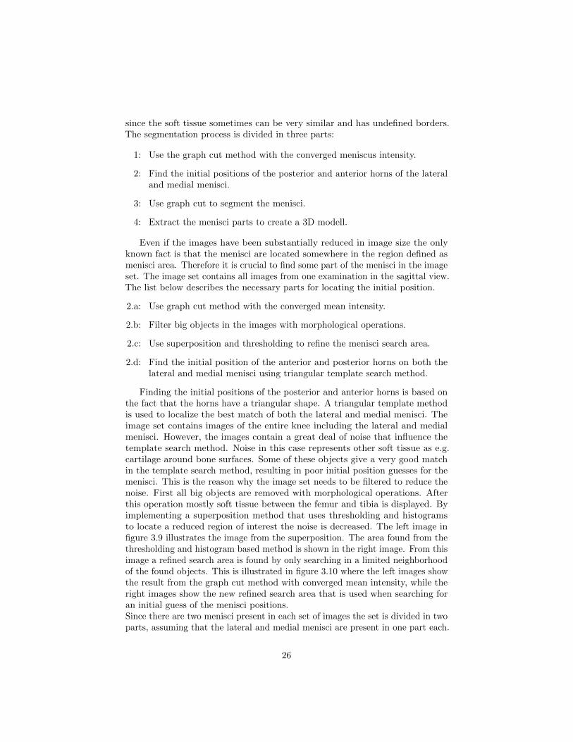
since the soft tissue sometimes can be very similar and has undefined borders.The segmentation process is divided in three parts:

1: Use the graph cut method with the converged meniscus intensity.

2: Find the initial positions of the posterior and anterior horns of the lateraland medial menisci.

3: Use graph cut to segment the menisci.

4: Extract the menisci parts to create a 3D modell.

Even if the images have been substantially reduced in image size the onlyknown fact is that the menisci are located somewhere in the region defined asmenisci area. Therefore it is crucial to find some part of the menisci in the imageset. The image set contains all images from one examination in the sagittal view.The list below describes the necessary parts for locating the initial position.

2.a: Use graph cut method with the converged mean intensity.

2.b: Filter big objects in the images with morphological operations.

2.c: Use superposition and thresholding to refine the menisci search area.

2.d: Find the initial position of the anterior and posterior horns on both thelateral and medial menisci using triangular template search method.

Finding the initial positions of the posterior and anterior horns is based onthe fact that the horns have a triangular shape. A triangular template methodis used to localize the best match of both the lateral and medial menisci. Theimage set contains images of the entire knee including the lateral and medialmenisci. However, the images contain a great deal of noise that influence thetemplate search method. Noise in this case represents other soft tissue as e.g.cartilage around bone surfaces. Some of these objects give a very good matchin the template search method, resulting in poor initial position guesses for themenisci. This is the reason why the image set needs to be filtered to reduce thenoise. First all big objects are removed with morphological operations. Afterthis operation mostly soft tissue between the femur and tibia is displayed. Byimplementing a superposition method that uses thresholding and histogramsto locate a reduced region of interest the noise is decreased. The left image infigure 3.9 illustrates the image from the superposition. The area found from thethresholding and histogram based method is shown in the right image. From thisimage a refined search area is found by only searching in a limited neighborhoodof the found objects. This is illustrated in figure 3.10 where the left images showthe result from the graph cut method with converged mean intensity, while theright images show the new refined search area that is used when searching foran initial guess of the menisci positions.Since there are two menisci present in each set of images the set is divided in twoparts, assuming that the lateral and medial menisci are present in one part each.

26

Figure 3.9: A superposition of all images is used to refine the search area for locatingthe initial positions of the lateral and medial meniscus. To the left theresult of the superpositioned images are shown. The intensity is based onhow often the pixel position is classified as meniscus from the previousgraph cut method. By thresholding these superpositioned images themost common pixel locations are located (right image). This method isused to localize the vertical position which is used to refine the searcharea when searching for the initial position of the meniscus.

One part is the images of the medial meniscus and the other part is containingimages of the lateral meniscus.

To locate the initial positions of the posterior and anterior horns a triangulartemplate search method is implemented. A template search method was usedto locate the best match to the anterior and posterior horns. This is done byassuming that the anterior horn is located somewhere to the left in the imageand the posterior horns somewhere to the right. The image with the best matchof both the posterior and anterior horns, as well as the initial positions of thehorns are saved. The initial position of the horns are calculated by taking thecenter of mass of the overlapping pixels between the image and the template,

The initial positions contain information about the positions of the anteriorand posterior horns of both the lateral and medial menisci in the 3D. This meansthat the image slice and the 2D coordinates for the menisci horns are known.An overview of the segmentation process is given in the list below and in figure3.11:

3.a: Use graph cut method with the converged mean intensity.

3.b: Extract the meniscus parts in the image using the initial positions.

3.c: Use the extracted meniscus parts to create a background map.

3.d: Use graph cut with the converged mean intensity and background map inthe nearby images.

3.e: Update the initial positions of the meniscus in the nearby images.

27

Figure 3.10: The left figure includes nine segmentation results from nine differentslices from the graph cut method with converged menisci mean intensity.These images contain noise such as cartilage around the femur andtibia. The noise will interrupt the localization of the initial positionsof the menisci. That is why the images are filtered with a thresholdingand histogram based method, see figure 3.9. The new search area isdisplayed in the right figure. Even if some noise is present the filterfunction will make the initial guess method more robust.

3.f: Return to 3.b until all images have been used.

The images of both the lateral and the medial menisci contain noise, whichdisturb the segmentation process. Therefore the segmentation process needsto gather information from the nearby images. Spacial distribution betweenthe images is very small, 3 mm in the examinations used in this work. Thismeans that the probability of finding the neighboring parts of the meniscus inthe nearby images is very high just by using the known meniscus position.

Figure 3.11 illustrates the segmentation process. The two images that gavethe best match in the triangular template search are used as an initial imagein the segmentation process i.e. the best initial guess for both the medial andlateral menisci. From this image the objects that interfered with the knowninitial positions are extracted creating an image known as the menisci image IM .The rest of the image is used as a background map. This map is used in thegraph cut method in the neighboring images. Objects in the background mapwill receive a high cost for being a meniscus part in the graph cut method. Thiswill lower the noise present in the images, in this case mostly cartilage.

The initial position is calculated for one specific image and can not be usedin all the other images. Therefore images created from the graph cut methodare compared against the menisci image IM in the previous slice. Objects thatinterfere between these images are used to create the menisci image for the newslice. The remaining objects are used to create a new background image. Thisprocess continues until all slices has been analyzed i.e. in all four directions, seefigure 3.12. As explained before the initial position contains the best match forboth the lateral and medial menisci. From each image this process is adapted

28

to the first or last image slice (depending on which is closest) and to the otherinitial position i.e. the segmentation process will generate two image sets.

From these four directions the menisci parts are extracted to create a visual3D object of the menisci. The problem of extracting these menisci parts liesin that two image sets are present, and to decide which of the images to usewhen creating the 3D object. As described earlier this segmentation process usesinterference between the graph cut images to decide what parts in the imagethat is classified as menisci. This implies that the initial position guess fromone of the meniscuses is needed to extract the menisci parts of that meniscus.From that point of view both of the initial positions are used to extract themenisci parts outwards from that starting point. However, the problem lies indetermining which of the images from the two image sets to use when extractingthe menisci parts between the initial positions. When searching inwards themenisci horns in the images are located and extracted. The problem lies infinding the endpoints of the anterior and posterior menisci parts. Either theendpoints are found when the search process can not find any menisci parts or itends when the search process finds the anterior or posterior ligaments. As seenin figure 1.4 the anterior and posterior cruciate ligament are located betweenthe medial and lateral menisci. In figure 4.4 the result from five examinationsare presented.

29

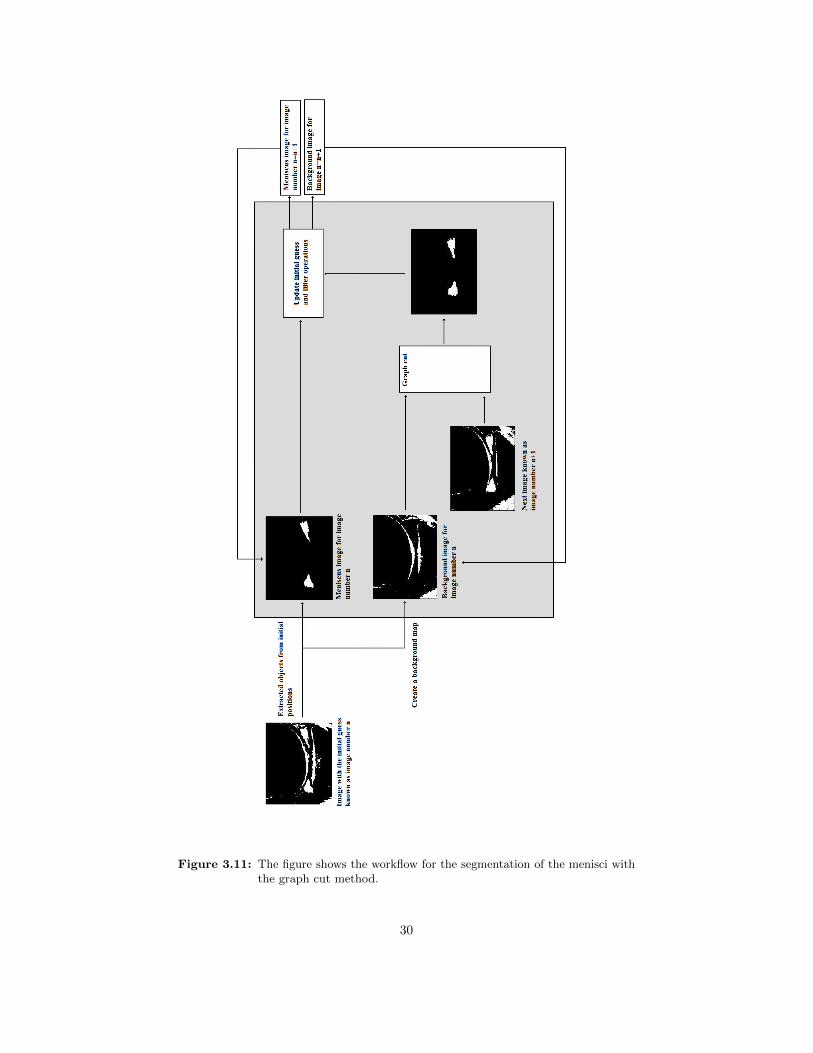
Figure 3.11: The figure shows the workflow for the segmentation of the menisci withthe graph cut method.

30

Figure 3.12: The small circles in the figure illustrate the two found initial position ofthe lateral and medial meniscus. From these position the search for theother parts of the menisci is done in the illustrated directions, i.e. totalyfour directions. From each initial guess a new image set will be createdcontaining the result from the segmentation process from concernedimages.

31

Chapter 4

Results

In this chapter the result from the different sub parts in the process of automat-ically segment the menisci is discussed. The workflow of this Masters’ thesiswas divided into three parts. The result from each part will be presented in onesection each.

4.1 Result of Bone Segmentation

The purpose of segmenting the bone was to reduce noise in the images. This wasdone with texture classification. Laws’ texture algorithm was used to extractfeatures from different textures. Other methods such as first order statisticsand Co-occurrence matrices with first order statistics were tried, cf. [2], with nosuccess. In this section the result from the bone segmentation is discussed andtherefore one essential part is how well the classification worked.

Some tissues and bone can be very similar and very hard to separate. Thisis visible in figure 4.1 where the left images illustrate the original MR imageand the right image displays the result from the classification process, knownas the probability map. The MR images approximately contain three textures.In the left image these textures are manually selected and classified as bone,bright tissue and dark tissue. As said earlier some texture is hard to separateand especially the textures bone and bright tissue. The result from how wellthe classifier works is presented in figure 4.2. The data is gathered from sixexaminations and contains approximately 4000 images from each of the threetexture types. These texture images are extracted manually from the MR imagesto compare the result from the classifier with the result given by the user. Theclassifier calculates a probability that the texture present in the image is bone.This means that textures that are not bone will have a small probability. Fromthis probability the system needs to decide a threshold value that can be used toclassify the textures as either bone or not bone. Therefore, the accuracy of theclassification for the three texture types is calculated against different thresholdvalues. The result is shown in figure 4.2. The accuracy is how many of the

32

texture images that has been accurately classified in the system with the giventhreshold value.

There are essentially two things to mention in the figure. First, note howwell the system works when differentiating the bone from the dark tissue in thethreshold interval 0.45-0.65. In this case the dark tissue and the bone accuracyis above 90%. Secondly, note how difficult it is to separate the bright tissue frombone. In the interval 0-0.65 the bright tissue has en accuracy under 10% andbone has en accuracy above 90%. In the interval 0.70-1 bright tissue has enaccuracy of above 90% and bone has an accuracy under 10%.

In the system the threshold was set to 0.5, see equation 3.2. One can arguethat it might be better to have a slightly higher threshold to increase the accuracyof the dark- and bright-tissue as the bone accuracy is slightly stabile. However,this is only slightly modifications and will not change the result remarkably.

Even if the classifier has problems to separate the bright tissue from the boneit does not impact the main objective to segment the menisci. These texturesare hard to separate but they do not look similar to the menisci and therefore itdoes not matter if the bright tissue is classified as bone as long as it does notinterfere with the menisci. So the objective is to segment the bone as well aspossible without erasing any valuable information regarding the menisci, andthis segmentation process works well with that objective.

Since the probability map is sufficiently accurate the graph cut methodworks very well. In figure 3.6 and 3.8 two examples of bone segmentation ispresented. From these figures it is visible how well the bone segmentation works.In figure 3.6 it is also visible that brighter tissue is classified as bone, but asexplained it does not matter since it is not similar to the meniscus textures andwill not be in danger for bad classifications regarding the menisci. In the imagein figure 3.8 the meniscus is zoomed in and the segmentation of bone aroundthe meniscus is shown clearly.

4.2 Result from Locating the Menisci Locations

The objective of the second part was to reduce the image size to be able to localizethe meniscus. This method is based on a superposition of the segmented boneimages. The method for locating the meniscus area is based on a thresholdingand histogram method of the superposition image. The result from this methoddepends on how well the bone classification went. Figure 4.3 shows the resultfrom four examinations. As seen in this figure the area where the menisci can belocated is found, often very well especially regarding the vertical position. Thehorizontal position is sometimes harder to find, see the lower image in the rightcolumn in figure 4.3. The purpose is still only to reduce the image size withoutloosing information regarding the menisci to simplify the segmentation process.

33

Figure 4.1: The left figure illustrates regions of the three different texture types darktissue, bright tissue and bone. To the right the image illustrates thecreated probability map where the intensity is based on how certain thesystem is that the region is bone. Note that the classifier can not separatethe bright tissue from the bone.

4.3 Segmentation Result of the Menisci

The third part was the segmentation of the menisci and this process is muchharder. The menisci and the cartilage in the neighborhood sometimes are jointtogether, see the lower image in the left column in figure 3.8. To lower theseeffects information from the nearest images is used to reduce this noise, seesection 3.3.2. This process reduces the noise in the images and this is necessarydue to the fact that the detected menisci objects is used to search for themeniscus in the nearby image. Noise will affect this search process and reducethe possibility to extract only real meniscus parts and create a 3D object of themenisci.

The segmentation result from five examination is shown in figure 4.4. In theimages the lateral as well the medial menisci are presented. The medial meniscusis the upper meniscus in the images. In the segmentation process more filteringoperations are needed to reduce the presence of cartilage when extracting thelateral menisci compared to the medial menisci. Therefore the medial meniscihave a more homogeneous surface. Even if there are filter operations to reducethe cartilage sometimes they do not remove all. In the lower image in columnone and the upper image in column two some cartilage is present. As discussedearlier the segmentation process uses information in the previous images toreduce noise. In some cases as the examination seen in column three, the imagequality is not good enough. If the intensity is too similar around the menisci thesystem can not segment the menisci parts and no result is achieved. In this casethe system can not distinguish the menisci from the rest of the image.

34

Figure 4.2: The figure illustrates how accurate the classification system works forthree texture types when changing the threshold value for being classifiedas bone resp. not bone. The three texture types is dark- and bright-tissueand bone.

35

Figure 4.3: In this figure the superposition results from four examinations is displayed.The white squares illustrates the located menisci area calculated with athreshold and histogram based method. Note that especially the verticalposition is found correctly and that the horizontal sometimes get a bitwider. However, the purpose of this calculation was to reduce the imagesize without loosing any information about the menisci.

36

Figure 4.4: In this figure the results from the 2D graph cut segmentation process ispresented. In most of the images both menisci are present. Note that thesegmentation result of the upper meniscus(medial meniscus) in most caseshas a meniscus shaped form. The result of the upper menisci in the thirdcolumn and the the lower image in the second column are not satisfactory.That is due to the fact that the images from the examination were notsharp enough and the system could not distinguish the meniscus in theimage. The lower menisci (lateral meniscus) are not as homogeneous asthe upper(medial meniscus). The segmentation process in the lateralmeniscus uses more filter operations to reduce the cartilage in the images.The cartilage is not always removed as seen in the lower image in columnone and in the upper image in column two.

37

4.4 Evaluation of the Results from the Auto-matic Segmentation

In this thesis the automatic segmentation is tested on five examinations. Toevaluate how good the result was Magnus Tagil at Department of Orthopedicsin Lund, manually segmented the menisci in four of the five examinations andone examination twice. The area from the automatic segmentation process wasthen compared to the resulting area of the manual segmentation.

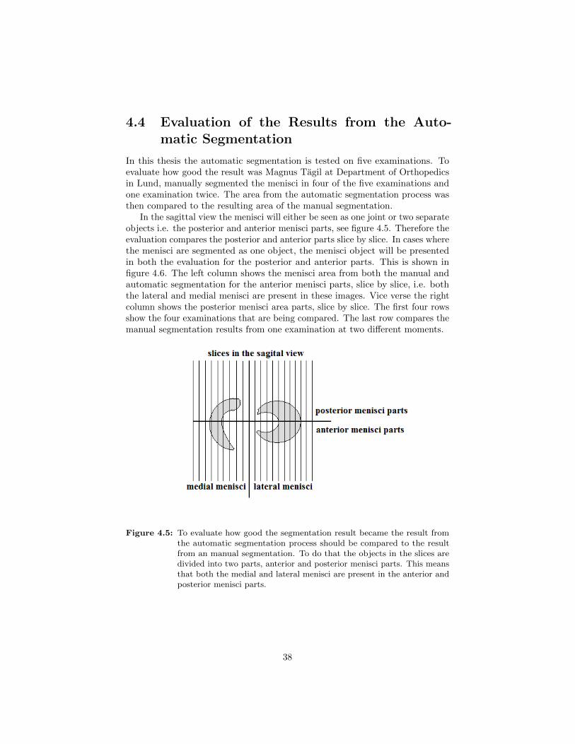
In the sagittal view the menisci will either be seen as one joint or two separateobjects i.e. the posterior and anterior menisci parts, see figure 4.5. Therefore theevaluation compares the posterior and anterior parts slice by slice. In cases wherethe menisci are segmented as one object, the menisci object will be presentedin both the evaluation for the posterior and anterior parts. This is shown infigure 4.6. The left column shows the menisci area from both the manual andautomatic segmentation for the anterior menisci parts, slice by slice, i.e. boththe lateral and medial menisci are present in these images. Vice verse the rightcolumn shows the posterior menisci area parts, slice by slice. The first four rowsshow the four examinations that are being compared. The last row compares themanual segmentation results from one examination at two different moments.

Figure 4.5: To evaluate how good the segmentation result became the result fromthe automatic segmentation process should be compared to the resultfrom an manual segmentation. To do that the objects in the slices aredivided into two parts, anterior and posterior menisci parts. This meansthat both the medial and lateral menisci are present in the anterior andposterior menisci parts.

38

4.4.1 Examination 1

The first row in figure 4.6 corresponds to the upper image in the left column infigure 4.4. In this case the initial guess for the medial meniscus is slice number5 and slice number 22 for the lateral meniscus. As seen in the left column theautomatic segmentation is slightly over segmented. In the right column theresult shows that the automatic segmentation has segmented objects in slicenumber 10-14 that has not been manual segmented. In this case the meniscihave an tubular structure that more or less links the medial and lateral meniscitogether. This is not really menisci parts, but the system can not differ theseobjects from the menisci. The result for the lateral meniscus is quite accurate inslice number 20-24. In figure 4.7 the segmentation result of slice number 5 isshown. The white objects is the result from the segmentation. The left imagecontains the result from the manual segmentation and the right the result fromthe automatic segmentation process. In this slice the segmentation result is verysimilar.

4.4.2 Examination 2

The second row in figure 4.6 belongs to the upper image in the second column infigure 4.4. Slice number 5 is the initial guess for the medial meniscus and slicenumber 18 is the initial guess to the lateral meniscus. As seen in these imagesthe system have over segmented the menisci. This is due to noise or cartilagewas present in these slices, especially in slice number 19-20 in the left columnand slice number 6-9 in the right column.

4.4.3 Examination 4

Row number three in figure 4.6 corresponds to the examination in the lowerimage in the first column in figure 4.4. The initial guesses are slice number 4and 21. The segmentation result shows that the automatic segmentation processalso had issues with noise or cartilage in this examination. This is seen in slicenumber 5-8 in the right column. Also observe how close the segmentation resultsare to each other in slice 20-25. Figure 4.8 contains the segmentation result forslice number 7. The left image contains the manual segmentation result and theright the automatic. In this case the automatic segmentation has segmented abigger area than the manual due to that automatic system can not distinguishthe cartilage from the meniscus.

4.4.4 Examination 5

The fourth row in figure 4.6 belongs to the lower image in the second column infigure 4.4 were the initial guesses are slice number 10 and 19. The segmentationresult is close to the manual segmentation result in slice number 4-9 in the leftcolumn and in 17-21 in the right column. The posterior meniscus parts from themedial meniscus is found in slice number 4-8 in the right column. In the same

39

slices the automatic segmentation could not find any menisci parts. The reasonis that the system could not distinguish the meniscus part in the image. This isdisplayed in figure 4.9 which displays the segmentation result of slice number 5.In the left image the manual segmentation result is shown and in the right theautomatic. In this case there are no posterior menisci parts segmented and thisis due to the diffuse meniscus boarders.

4.4.5 Examination 5 again

The last row in figure 4.6 shows the manual segmentation result from oneexamination produced at two different times. The interesting part is howdifferent the result became. In this case the area variation differs a lot in someslices, almost 50% in slice number 20 in the right column. Also observe thedifference in slice number 10 and 17 in the left column where menisci parts isfound in one examination but not in the other. This shows how difficult thesegmentation task really is and how much an accurate automatic segmentationprocess could help future diagnoses.

4.4.6 Summary

Overall the segmentation system is quite accurate in the neighborhood of theinitial guesses. The system is not perfect and has some issues with cartilageand noise, in some slices, and deciding when to stop the search process. Inseveral slices the segmentation has continued when the manual segmentation hasstopped.

40

Figure 4.6: In this figure the area between the manual and automatic segmentationis displayed.

41

Figure 4.7: This image shows the segmentation result of the initial guess in examina-tion 1, slice number 5. The left image shows the result from the manualsegmentation and the right the automatic. The segmentation result isplotted as white objects. Please note that the images have different scalesbecause the manual segmentation was done in an external program.

42

Figure 4.8: The left image shows the manual segmentation of slice number 7 inexamination 4. In the right image the segmented area from the automaticsegmentation is shown. The segmentation result is plotted as whiteobjects. Please note that the images have different scales because themanual segmentation was done in an external program. In this casethe segmentation result have had trouble with distinguish the meniscusboarders, which resulted that bigger area was segmented.

43

Figure 4.9: The manual segmentation result for slice number 5 in examination 5 isshown in the left image. The result is displayed as white objects in boththe left and right image. In this case the automatic segmentation couldnot segment the posterior meniscus part, see the right image. This isdue to the diffuse boarders of the meniscus. Note that the images havedifferent scales.

44

Chapter 5

Future work

The approach to automatically segment the menisci in this Masters’ thesis usessome different search methods and these can be very time consuming in Matlab.This program was not constructed to be very fast, but as an improvement thesearch methods could be written in a faster programming language.

At the moment the program is constructed to work with MR images withthe image acquisition discussed in section 1.3. This means that the training dataused when segmenting bone is limited to this image acquisition. More trainingdata could make this program work with additional examinations with otherimage acquisitions.

As discussed in the result chapter the whole workflow demands that the bonesegmentation works well. To improve this segmentation the classifier could betested for optimization. Perhaps not all 71 features are necessary to use andperhaps a better result would be achieved by replacing the k-nearest neighborwith another classifier such as support vector machine [1, page 523-527].

At the moment the segmentation process used is a bit complex. One problemwith the segmentation process used in this thesis is that cartilage interfere withthe segmentation process and influences the result. Perhaps a better result couldbe achieved with a 3D graph cut segmentation. Usually the cartilage aroundthe tibia are joined together with the menisci, as seen in lower image in the leftcolumn in figure 3.8. This will of course influence the result in the segmentationprocess. A 3D graph cut segmentation might reduce this phenomena since thecartilage shape is thin and wide and might be limited in the regularization term.This could result in a more accurate segmentation. Even better result wouldprobably be achieved if the segmentation system used graph cut with shapepriors. The menisci has a known shape and that could be used to create shapepriors. Another approach would be to modify the existing program by updatingthe mean intensity in every slice before the graph cut segmentation. This couldperhaps result in a more accurate segmentation. The segmentation process inthis thesis uses a calculated converged mean intensity of the meniscus in thesegmentation process for all slices.

The main objective is to use the 3D object to determine if the menisci are

45

healthy or not. This would involve a pattern recognition system to classify themenisci as healthy or not. Some studies have already been done that can be usedas an inspiration to suitable features that can be used in such classifications, cf.[21]. Features of interest would most certain be features like the volume, surfaceand determine if the menisci horns are sharp or truncated. The features wouldprobably depend on factors like gender, age and body mass.

46

Bibliography

[1] David A.Forsyth and Jean Ponce. Computer Vision: A Modern Approach.Alan Apt, 2003.

[2] E. Alegre, V. Gonzalez-Castro, S. Suarez, and M. Castejon. Comparisonof supervised and unsupervised methods to classify boar acrosomes usingtexture descriptors. 2009 International Symposium ELMAR, pages 65–70,2009.

[3] I. Boniatis, G. Panayiotakis, and E. Panagiotopoulos. A computer-basedsystem for the discrimination between normal and degenerated meniscifrom Magnetic Resonance images. 2008 IEEE International Workshop onImaging Systems and Techniques, pages 335–339, 2008.

[4] Y. Boykov and R. Veksler, O. Zabih. Fast approximate energy minimizationvia graph cuts. IEEE Transactions on PAMI, 23(11):1222–1239, 2006.

[5] Yuri Boykov and Vladimir Kolmogorov. Implementation of maxflow-v3.01,2010. http://www.cs.ucl.ac.uk/staff/V.Kolmogorov/software.html.

[6] M.D Crema, A Guermazi, L. Li, M.H Nogueira-Barbosa, and et al. Theassociation of prevalent medial meniscal pathology with cartilage loss in themedial tibiofemoral compartment over a 2-year period. Osteoarthritis andCartilage, 18(3):336–343, 2010.

[7] Omer Demirkaya, Musa Hakan Asyali, and Prasanna K.Sahoo. ImageProcessing with MATLAB, Applications in Medicine and Biology. BocaRaton : CRC Press, 2009.

[8] J. Fripp, P. Bourgeat, C. Engstrom, S. Ourselin, S. Crozier, and O. Salvado.Automated segmentation of the menisci from MR images. 2009 IEEEInternational Symposium on Biomedical Imaging: From Nano to Macro,pages 510–513, 2009.

[9] J Fripp, S Crozier, S.K Warfield, and S. Ourselin. Automatic segmentationof articular cartilage in magnetic resonance images of the knee. IEEETransactions on Medical Imaging, 29:55–64, 2010.

47

[10] Jurgen Fripp, Stuart Crozier, Simon Warfield, and Sebastien Ourselin.Automatic segmentation of the bone and extraction of the bone-cartilageinterface from magnetic resonance images of the knee. Physics in Medicineand Biology, 52(6):1617ı£¡1631, 2007.

[11] Y. Hata, S. Kobashi, Y Tokimoto, M. Ishikawa, and H. Ishikawa. ComputerAided Diagnosis System of Meniscal Tears with T1 and T2 Weighted MRImages Based on Fuzzy Inference. Computational Intelligence. Theory andApplications, LNCS 2206:55–58, 2001.

[12] Klas Josephson. Segmentation of Magnatic Resonance Images of the Kneeusing Tree-dimensional Active Shape Models. Master’s thesis, Dept. ofMathematics, Lund Institute of Technology,Sweden, 2004.

[13] V. Kolmogorov and R. Zabih. What energy functions can be minimized viagraph cuts? IEEE Transactions on PAMI, 26(2):147–159, 2004.

[14] C. Kose, O. Gencalioglu, and U. Sevik. An automatic diagnosis method forthe knee meniscus tears in MR images. Expert Systems with Applications,36(2):1208–1216, 2009.

[15] Ian D. McDermott. What tissue bankers should know about the use ofallograft meniscus in orthopaedics. Cell and Tissue Banking, 11(1):75–85,2010.

[16] B. Paniagua-Paniagua, M.A. Vega-Rodriquez, and P. Bustos-Garcia. Ad-vanced TextureAnalysis in Cork Quality Detection. 2007 5th IEEE Interna-tional Conferance on Industrial Informatics, pages 311–315, 2007.

[17] R. Pfisterer and F. Aghdasi. Comparison of texture based algorithms forthe detection of masses in digitised mammograms. AFRICON, 1999 IEEE,1:383–388, 1999.

[18] M. Rachidi, C. Chappard, A. Marchadier, C. Gadois, and et al. Applicationof Laws’ masks to bone texture analysis: An innovative image analysis toolin osteoporosis. 2008 5th IEEE International Symposium on BiomedicalImaging: From Nano to Macro, pages 1191–1104, 2008.

[19] M.T Suzuki, Y. Yaginuma, and H. Kodama. A texture energy measurmenttechnique for 3d volumetric data. 2009 IEEE International Conference onSystems, Man and Cybernetics, pages 3779–3785, 2009.

[20] M.S. Swanson, J.W. Prescott, T.M. Best, K. Powell, R.D. Jackson, F. Haq,and M.N. Gurcan. Semi-automated segmentation to assess the lateralmeniscus in normal and osteoarthritic knees. Osteoarthritis and Cartilage,18(3):344–353, 2010.

[21] W. Wirth, R.B. Frobell, R.B. Souza, X. Li, B.T. Wyman, M.P Le Graverand,T.M. Link, S. Majumdar, and F. Eckstein. A three-dimensional quantitativemethod to measure meniscus shape, position, and signal intensity using

48

mr images: a pilot study and preliminary results in knee osteoarthritis.Magnetic resonance in medicine, 63(5):1162–1171, 2010.

[22] Donald W.McRobbie, Elizabeth A. Moore, Martin J. Graves, and Martin R.Prince. MRI from picture to proton. printed in the United Kingdom at theuniversity Press, Cambridge., second edition, 2008.

49