Automatic segmentation and classication of seven-segment ......Automatic segmentation and...

Automatic segmentation and classification of seven-segment displaydigits on auroral imagesT. Savolainen1, D. K. Whiter2,3, and N. Partamies2,4

1Aalto University, Helsinki, Finland2Finnish Meteorological Institute, Helsinki, Finland3University of Southampton, UK4University Centre in Svalbard, Norway

Correspondence to: T. Savolainen ([email protected])

Abstract. In this paper we describe a new and fully automatic method for segmenting and classifying digits in seven-segment

displays. The method is applied to a data set consisting of about 7 million auroral all-sky images taken during the time period

of 1973-1997 at camera stations centered around Sodankylä observatory in Northern Finland. In each image there is a clock

display for the date and time together with the reflection of the whole night sky through a spherical mirror. The digitised film

images of the night sky contain valuable scientific information, but are impractical to use without an automatic method for5

extracting the date-time from the display. We describe the implementation and the results of such a method in detail in this

paper.

1 Introduction

Aurora light is a result of interactions between charged particles and atmospheric atoms and molecules. Guided by the Earth’s

magnetic field, charged particles of magnetospheric and solar origin deposit their excess energy in circular zones around the10

magnetic poles. On the night side of the Earth, this so called auroral oval is typically observed at magnetic latitudes of about

65-75 degrees (Nevanlinna and Pulkkinen, 2001) but its width and brightness varies with solar activity and processes in near-

Earth space (Nevanlinna and Pulkkinen, 1998; Partamies et al., 2014). Analysis of the structural and temporal changes in the

aurora thus provides information on processes in the magnetospheric source region of the precipitating particles as well as

information on the terrestrial responses to space weather events. The auroral emissions are produced at about 100-200 km15

above the ground, and the most intense emission is typically an atomic oxygen emission line at 557.7 nm (green, often visible

to human observers).

Systematic ground-based imaging of the aurora by the Finnish Meteorological Institute started in 1973, and for two solar

cycles (1973-1997) a total of 8 all-sky colour film cameras were operated at stations across Finland and at Hornsund, Svalbard.

The same type of cameras were operated by other institutes during the same time period in four other locations: Tromsø and20

Andøya (Norway), Kiruna (Sweden) and Georg Foster (Antarctica). Typically a 20 second exposure was taken by each camera

once per minute. Towards the end of the 20th century the film cameras were replaced with digital imagers and incorporated

into the MIRACLE network (Syrjäsuo et al., 1998). These new instruments provide data in a format which can be readily

1

Geosci. Instrum. Method. Data Syst. Discuss., doi:10.5194/gi-2015-28, 2016Manuscript under review for journal Geosci. Instrum. Method. Data Syst.Published: 19 January 2016c© Author(s) 2016. CC-BY 3.0 License.

analysed using computer programs. To extend the digital auroral image database of the MIRACLE network of all-sky cameras

(ASCs)(Sangalli et al., 2011; Rao et al., 2014) the data from the film cameras were recorded to VHS tapes for easier access,

and later digitised into MPEG video format. In this paper we document an automatic number recognition method developed

for reading the digits in an LED clock display visible in the digitised film camera images. This method has been applied to

data from 1973-1997 from the 7 Finnish camera stations and the one in Hornsund, Svalbard. The process is important because5

it allows us to add two full solar cycles to the length of the digital image time series, which starts in 1996. We aim to make the

film camera data accessible to the scientific community.

Many of the classification methods found in the literature work exceptionally well for segmented datasets such as the Mixed

National Institute of Standards and Technology (MNIST) data set (Li, 2012). Applying these techniques to real auroral camera

data is not straightforward for several reasons. Optical data obtainded outdoors is rarely of such a high quality that the images10

can easily be segmented into sub images that contain only the pixels of the clock display digits. Long time series consist of

vast amounts of data, which makes it impractical to have a training set containing half of the data set. The reason for using

automatic methods in the first place is the fact that the labelling of the data is costly and laborious.

Automatic segmentation is by definition based on some a priori data. These data can be segmented images for training a

supervised learning algorithm, or hand calculated statistics for threshold based methods or other features found in the data set.15

Ideally this a priori knowledge should be as generic as possible to make it applicable to a wide variety of data and as accurate

as possible to minimise the error in the segmentation.

In addition to solving the segmentation problem, the a priori knowledge has to be formulated in mathematical terms and

discretized to make it computable. The computational complexity and system runtime of the algorithm are important to enable

fast testing and data extraction.20

To address these challenges we describe a new method that:

1. Incorporates the a priori knowledge of the display geometry as a template

2. Detects if the image has a display with digits

3. Finds the midpoints of the digits in the display and extracts the digits

4. Determines the scale and the intensity of the digits and normalises them25

5. Uses a combination of Principal Component Analysis (PCA) and K-Nearest Neighbours (KNN) techniques to classify

accurately the individual numbers with only ∼ 0.1% of the data set as a training set

6. Has small memory requirements and processes 24 images/s on modest hardware in 2015

7. Works well with noisy and low resolution images

2


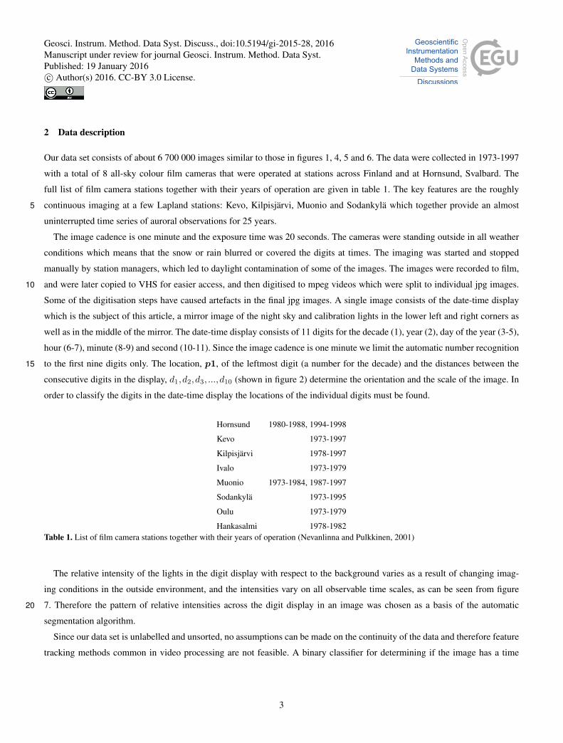
2 Data description

Our data set consists of about 6 700 000 images similar to those in figures 1, 4, 5 and 6. The data were collected in 1973-1997

with a total of 8 all-sky colour film cameras that were operated at stations across Finland and at Hornsund, Svalbard. The

full list of film camera stations together with their years of operation are given in table 1. The key features are the roughly

continuous imaging at a few Lapland stations: Kevo, Kilpisjärvi, Muonio and Sodankylä which together provide an almost5

uninterrupted time series of auroral observations for 25 years.

The image cadence is one minute and the exposure time was 20 seconds. The cameras were standing outside in all weather

conditions which means that the snow or rain blurred or covered the digits at times. The imaging was started and stopped

manually by station managers, which led to daylight contamination of some of the images. The images were recorded to film,

and were later copied to VHS for easier access, and then digitised to mpeg videos which were split to individual jpg images.10

Some of the digitisation steps have caused artefacts in the final jpg images. A single image consists of the date-time display

which is the subject of this article, a mirror image of the night sky and calibration lights in the lower left and right corners as

well as in the middle of the mirror. The date-time display consists of 11 digits for the decade (1), year (2), day of the year (3-5),

hour (6-7), minute (8-9) and second (10-11). Since the image cadence is one minute we limit the automatic number recognition

to the first nine digits only. The location, p1, of the leftmost digit (a number for the decade) and the distances between the15

consecutive digits in the display, d1,d2,d3, ...,d10 (shown in figure 2) determine the orientation and the scale of the image. In

order to classify the digits in the date-time display the locations of the individual digits must be found.

Hornsund 1980-1988, 1994-1998

Kevo 1973-1997

Kilpisjärvi 1978-1997

Ivalo 1973-1979

Muonio 1973-1984, 1987-1997

Sodankylä 1973-1995

Oulu 1973-1979

Hankasalmi 1978-1982Table 1. List of film camera stations together with their years of operation (Nevanlinna and Pulkkinen, 2001)

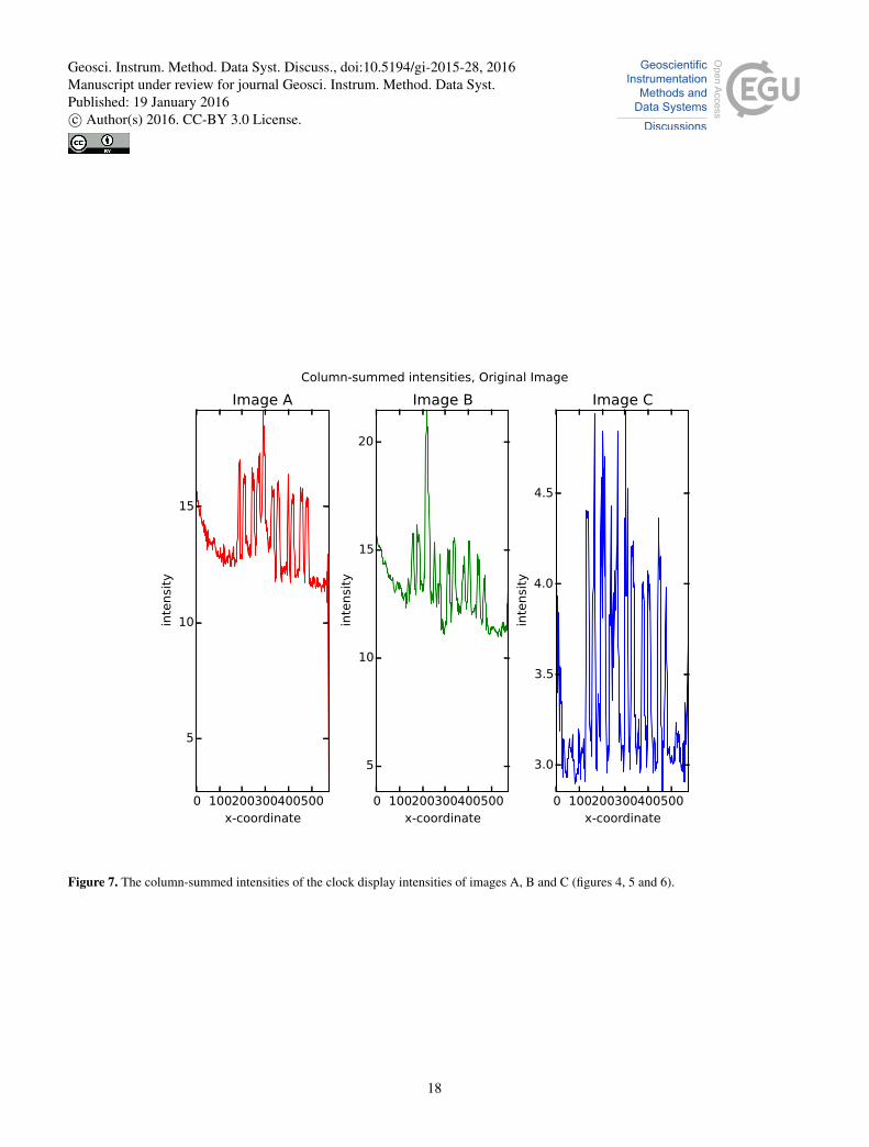
The relative intensity of the lights in the digit display with respect to the background varies as a result of changing imag-

ing conditions in the outside environment, and the intensities vary on all observable time scales, as can be seen from figure

7. Therefore the pattern of relative intensities across the digit display in an image was chosen as a basis of the automatic20

segmentation algorithm.

Since our data set is unlabelled and unsorted, no assumptions can be made on the continuity of the data and therefore feature

tracking methods common in video processing are not feasible. A binary classifier for determining if the image has a time

3


display is needed. Only ∼ 50% of all images had a visible and human readable display. The flow chart of the data conversion

process is summarised in figure 3.

In the following sections our display template refers to a collection of manually calculated values from a single representative

image. These include the approximate size of the digits (in pixels), the pattern of relative distances and approximate size of the

digit plate, all calculated from the template image (figure 1).5

3 Problem description

The purpose of the algorithm described here is to accurately predict the values of the first nine digits in the image. The problem

is formulated as follows: We begin with an image A with dimensions of 576x720 pixels. Each pixel of the image has three

colour components (R=red, G=green, B=blue). Since the colours in the image are not calibrated, we are only interested in the

intensity of the pixels (Y). The intensity can be calculated as the Y component of the CIE 1931 colour space (Hill B. et al. ,10

1997):

Y (R,G,B) = 0.2125R+ 0.7154G+ 0.072B (1)

The task is then to find the labels for the first nine digits in the image. These labels can be represented by the label vector

L = {l1, l2, l3, l4, l5, l6, l7, l8, l9}. Given the matrix (image) A we want to estimate labels in such a way that the classification

error:15

E = P (L 6= L), where L = estimate for the label (2)

is minimised. This problem can be divided into sub problems that can be solved independently. In our method we divide the

problem into three phases:

1. Phase I: Does the image have a digit display? If it has a digit display, what is the location of the display?

2. Phase II: Does the geometry of the display correspond to the template? If it does, which pixels in the image correspond20

to the digits?

3. Phase III: Given a feature vector corresponding to the pixels of the digit determine the appropriate class (value) for the

digit.

Phase I: Given a real valued matrix A representing the intensities of the 2D-image determine if the distances d1, ...d10 (figure

2) satisfy the condition: d1,d3,d4,d6,d8,d10 < d2,d5,d7,d9. If the criterion is met the coordinates of the bottom left corner of25

the clock display (p1x, p1y) (figure 2) are given as input to phase II.

Phase II: In a real valued matrixD corresponding to the pixels of the date-time display in the image, we find position vectors

p1,p2, ...p11 which describe the midpoints of the digits in screen coordinates, with the following criteria:

1. 0.7τi ≤mi ≤ 1.35τi

4


2.∑10

i=1 di > 100

where mi = di∑10j=1 dj

, i= 1,2, ...,10 and τi are the digit distance values di in the template image.

Phase III: Sub-sets of pixels corresponding to each digit are extracted from the matrix A when position vectors pi, the width

of the digits w and the width-to-height ratio are known from the template and defined by the above criteria. Feature vectors are

constructed from the pixels of individual digits. A classifier then assigns a label (value) to each extracted digit based on this5

feature vector.

4 Previous work

Seven-segment displays are found on calculators, digital watches, as well as audio and video equipment(Bonacic et al., 2009).

Automatic means of segmenting the displays and recognition of the digits would enable automation of many laborious tasks.

The recognition of segmented handwritten digits has also been widely studied (Li, 2012; Oliveira et al., 2002).10

With the advent of computational power some effort has recently been put into detecting numbers in digital displays. Some

of the problems associated with segmenting numbers in digital displays are low contrast, high contrast, bleeding and specular

reflections (Tekin et al., 2011). In addition to these general view point dependant features our data set suffers from the variable

weather and light conditions and multi-step digitisation.

Existing recognition algorithms for classifying digits typically perform with about 99% accuracy with hard to read hand15

written digits (Salakhutdinov and Hinton, 2007). These algorithms are applicable to seven-segment displays as well.

Segmentation and specifically fully automatic segmentation algorithms are built on a priori knowledge about the data set.

The simplest ones include plenty of experimentally obtained threshold values such as average intensity in a specific region

(Sezgin M. and Sankur B. , 2004). Threshold based methods work well on small homogeneous sets but not on large data sets,

mainly because obtaining threshold values experimentally is time-consuming and a fixed parameter often poorly describes the20

entire data set. Consider an LED screen for a single hour of images. During this hour the intensity of the screen can be steadily

20% brighter than the background. It is then easy to find a threshold value that makes the algorithm work with almost 100%

accuracy. However, the assumption that the intensity is above this threshold value is probably not true for the next hour, day or

especially during full moon or foggy conditions.

5 Methods and analysis25

In this section we describe in detail the three phase process used for segmenting and detecting the clock display digits in the

images. Phases I and II are more task specific and incorporate more a priori information than phase III, which could be changed

to a more suitable multiclass classification algorithm depending on the particular data set.

5


5.1 Phase I: binary classification

The purpose of phase I is to determine if the image has digits or not. This is important since in some of the images extracted

from the digitised films the clock display is not visible at all, for example the camera mirror and the display may be covered in

snow or saturated by the light of the full moon. The optimal binary classifier should have both 0% false negative probability

(classifying images with digits as images not having digits) and 0% false positive probability (classifying images not having5

digits as having digits). It was decided that it is most important to minimise the former probability in order not to miss useful

data and therefore a moderately strict classifier is needed.

The classification in both phases I and II is based on four assumptions:

1. The relative distances and shapes of the numbers follow the template of the display within the range defined by the Phase

II criteria in section 3.10

2. The 11 highest local maxima in the column-summed intensities (equation 3 below) correspond to the midpoints of the

digits.

3. The display and the numbers are approximately aligned horizontally

4. The number of digits is 11

With these assumptions the task of determining if the image has eleven digits is a task of finding the pattern of eleven15

intensity maxima in the image.

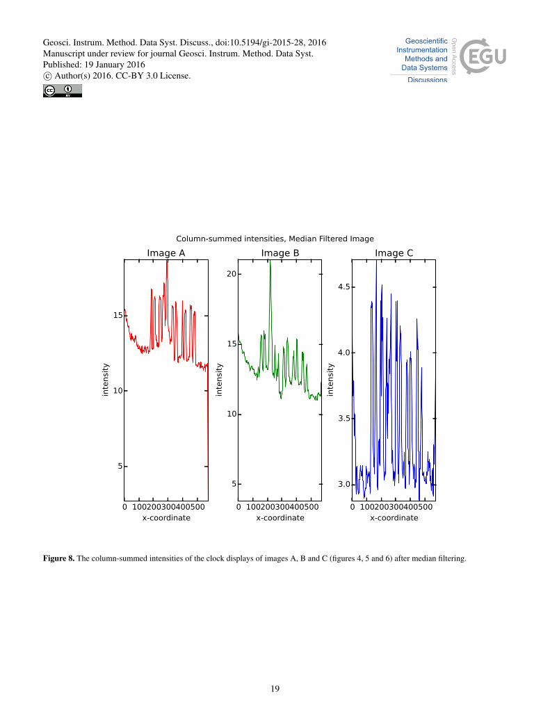
Before a binary classification is done the image is median filtered. The median filter removes some noise from the original

image; the difference can be seen by comparing the column-summed intensities (equation 3) of the original image (figure 7)

and the median filtered image (figure 8)

The actual classification works as follows:20

1. Consider each row of the image as a one dimensional signal

2. Start from the first row (i= 1)

3. Take 10 rows at a time

4. Sum the values of the ten rows to get a new signal

5. Normalise this signal by calculating the mean and subtracting it from the signal25

6. Save the first 16 nonzero values to a list

7. If the distances between the highest 11 of the 16 follow the pattern slsslslsls, where s = short, l = long, then the signal is

valid and the digit pattern has been found.

8. If the signal was valid mark it to a result array as valid

6


9. Go to the row i+ 1 and repeat steps 3-8 until row n− 10, where n is the number of rows

10. If the number of valid rows is 10 or greater then the image is classified as having digits

11. The digit display location in the y-direction is calculated as the mean location of the rows that matched the pattern.

5.2 Phase II: midpoint detection

Phase I estimates the location of the display, without considering its size. The purpose of phase II is to extract the width,5

height and the location of the midpoints of the individual digits. The assumptions made in phase I apply also here. Additional

assumptions are:

1. The number of peaks in the filtered column-summed intensities is exactly 11 (the number of digits)

2. The width to height ratio of the digits is 0.7 i.e. the width = 0.7 ∗ height

3. The numbers have relative distances determined by the template pattern, equal to [0.0, 0.076, 0.136, 0.076, 0.076, 0.136,10

0.076, 0.136, 0.076, 0.136, 0.076].

4. Each relative distance can vary in the range [d ∗ 0.7, d ∗ 1.35], where d= distance

5. The distance between the midpoint of the rightmost digit and the midpoint of the leftmost digit is greater than 100 pixels

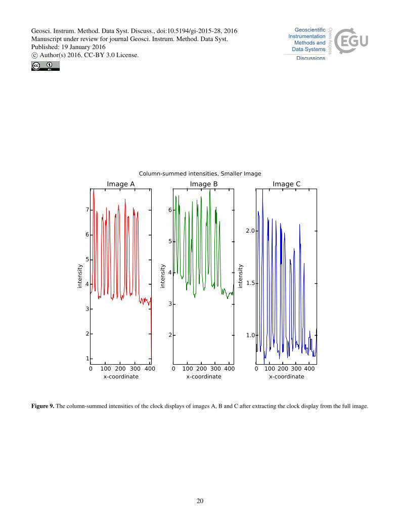
In phase II we calculate column-summed intensities of the display by summing over Y-axis values of the intensity matrix

(image) D:15

σ(x) =∑

y

D(x,y) (3)

The column-summed intensities of images A, B and C (shown in figures 4, 5 and 6) can be seen in figure 9.

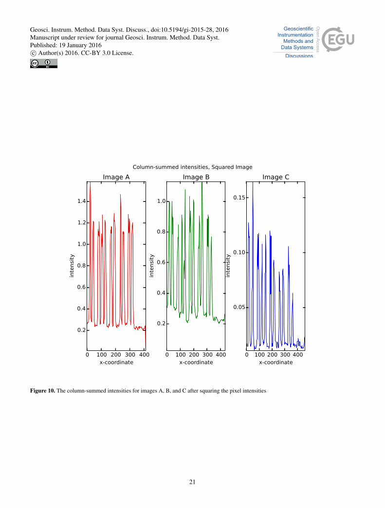
In phase II the following steps are done in order:

1. Raise every intensity value to the second power, see figure 10

2. Calculate the column-summed intensities according to equation 320

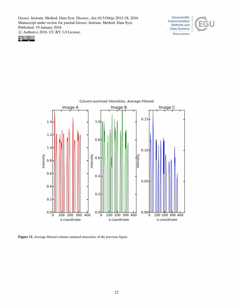
3. Set values below the mean to 0, see figure 11

4. Estimate a common width for all digits as the mean width of the 3rd, 4th and 5th largest widths of all digits

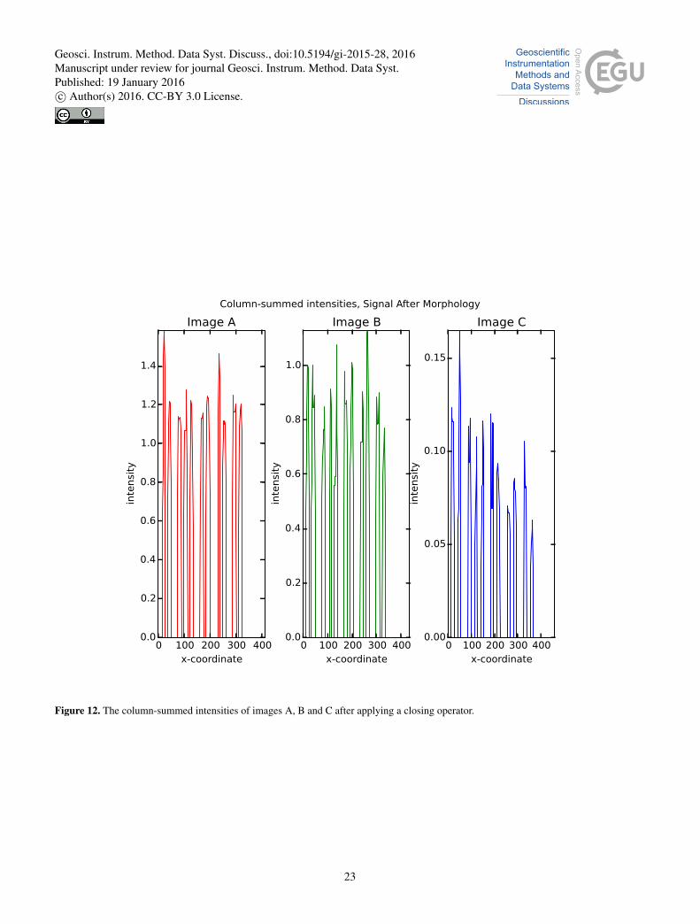
5. Apply a closing operator (a morphological operator filling real data gaps) with a sliding window, using the estimated

common width as a parameter, see figure 12

6. Find the midpoints of non-zero regions in the horizontal direction25

7


7. Find the location of the midpoints in the vertical direction:

(a) Sum the x-values around the midpoints.

(b) Set values below the mean to 0

(c) Estimate the midpoint in the vertical direction as the midpoint of the first nonzero region in the row-summed

intensities5

8. Scale the digits to 16x24 pixels (based on the template) with bilinear interpolation

9. Normalise intensities linearly from 0 to 255

The automatically segmented and normalised images corresponding to original figures 4, 5 and 6 can be seen in figures 13,

14, 15 respectively.

5.3 Phase III: digit classification10

Each digit is scaled to 16×24 pixels in steps 8 and 9 of phase II, which corresponds to a feature vector with 384 dimensions

per digit. The purpose of phase III is to determine the class (integer in range [0,9]) based on these numerical values. Because

the digits have undergone a multitude of linear and nonlinear transforms in the process, the digits differ significantly from the

original typeface. It is therefore necessary to use supervised learning; in our case we chose the k-nearest neighbours (KNN)

algorithm for its simplicity and speed. In conjunction with KNN we used principal component analysis (PCA) to reduce the15

dimensionality of the problem from 384 to 16. The eigenspace of the digits with only 16 dimensions was able to explain

98% of the variance of the original 384 dimensional space. This is intuitively clear since ideally there are only 7 degrees of

freedom in seven-segment displays. The KNN algorithm was trained in the 16-dimensional eigenspace with 42493 examples,

corresponding to about 0.1% of the whole data set. The following assumptions were made in this phase:

1. The possible classes of digits are restricted according to the following a priori knowledge:20

l1 ∈ {7,8,9} decades

l2 ∈ {0,1,2,3,4,5,6,7,8,9} years

l3 ∈ {0,1,2,3} hundreds of days

l4 ∈ {0,1,2,3,4,5,6,7,8,9} tens of days

l5 ∈ {0,1,2,3,4,5,6,7,8,9} days

l6 ∈ {0,1,2} tens of hours

l7 ∈ {0,1,2,3,4,5,6,7,8,9} hours

l8 ∈ {0,1,2,3,4,5} tens of minutes

l9 ∈ {0,1,2,3,4,5,6,7,8,9} minutes

This corresponds to the knowledge that the time series consists of images taken between 1973 and 1997, the fact that

there are at most 366 days in the year, that the day has 24 hours and an hour has 60 minutes.

8


2. Zero rejection rate: all feature vectors will be assigned a label.

3. The predicted dates and times are assumed to be reasonable within the above mentioned restrictions, i.e. there is no

additional checking for dates like 70 388 27 52 (yy doy hh mi).

6 Results and discussion

The algorithm presented here was developed in order to automatically read the date-time meta data for a 25-year time series of5

images of aurora. Four measures were used to determine the performance of the algorithm.

1. The recognition error, i.e. the number of correctly classified consecutive digits in images which include a clock display.

Since labelling low quality digits has some ambiguity, lower and upper limits are given. The lower limit corresponds to

labelling all unclear digits (to a human observer) as wrongly classified and the upper limit corresponds to labelling digits

as correct if the algorithm’s classification seems like the best guess. This step was performed by all 3 authors as human10

experts visually examining the images.

2. The probability that an image has digits if it was classified as having digits.

3. An estimate of the amount of useful data missed by the algorithm. This step is done by visually inspecting the data.

4. The approximate system run time per image.

The success of the recognition was defined as correct segmentation and classification of the first n digits in the display.15

This measure is based on the fact that the first digits are more significant in determining the time stamp of the image. The

recognition error was estimated by selecting a random sample of 1000 images from the 3000000 images that were classified as

having digits and comparing the computer predictions to the original unprocessed images, see table 2.

n or more correct 9 8 7 6 5 4 3 2 1 0

lower estimate 571 783 816 843 848 876 906 923 954 1000

higher estimate 951 959 964 973 976 982 989 989 999 1000Table 2. Number of images with at least n correctly classified digits out of nine. The sample of 1000 images were manually viewed by all

authors independently.

The probability of a false positive result was estimated from the same random sample as the recognition rate. For estimating

the probability of a false negative result a considerably larger data set consisting of several winters of rejected data from20

different decades was manually examined. Of this sample only 26954 (7.46%) images had digits which were human readable.

Most of the rejected images that had human readable numbers contained contaminating light: moon reflection, sunrise or

sunset, or bright aurora. Other common reasons for rejection include problems with the LED display (too bright or too dim

or unevenly bright) and artifacts resulting from the digitisation process (extra stripes of light, badly synchronised video etc.,

9


which make the search routine for the clock display pattern fail. Based on these observations the algorithm seems to capture

most of the useful data. A summary of the assessment of the algorithm is shown in table 3.

total number of images 6700000

total number of classified images 3000000

classified images which do have numbers (true positives) 100%

rejected images which contain human readable numbers (false negatives) 7.46%Table 3. True positives vs false negative error rates in detecting the clock display of all digitised images.

From a computational point of view the algorithm performed quickly; the whole data set was processed over one weekend.

Measurements of the total run time are given in table 4. Most of the software was written in the Python language using the

Scipy library (Oliphant, Travis E., 2007), but the most time consuming parts were written in C in order to improve performance.5

The computation speed is mostly limited by the read and write speeds of the computer disks. Since the images are processed

individually the program should be easily parallelizable by dividing the image set between multiple storage locations and

starting separate processes in each location. The computation speed was estimated using a mid-2014 Mac Book Pro Retina

computer with 2.6 GHz dual-core Intel Core i5 processor and 8 GB of 1600 MHz DDR3L onboard memory with a 256 GB

PCIe-SSD hard drive.10

number of images total run time (s)

1000 73.91

10000 417.89Table 4. Run times for the digit detection algorithm using a mid-2014 Mac Book Pro computer

7 Conclusions

In this work we describe a general method for processing images of varying quality using pattern matching and other signal

processing techniques in order to automatically determine the digits displayed in a seven-segment display. The algorithm

performs at or above the level of human recognition. It was able to recognise almost all of the digits of good quality, while

becoming increasingly uncertain with decreasing quality of the images. Since it is hard for human experts to classify the low15

resolution and blurred digits, it is hard to evaluate further improvement of the classification. Good results were obtained both

with respect to classification error and run time.

Even though the method was tailored for a specific problem it is applicable to other related segmentation problems as well.

The algorithm could be used to process similar old data stored at other research institutes with minor modifications, such

as adjusting the template describing the digit display. Based on the results of this study the digitisation of photographic film20

containing old data is a crucial process worth doing well in order to keep the data quality as high as possible.

10


The algorithm could be improved by

considering the rotation of the images, since only small rotations (±5◦) are handled by the current program. One way to

further improve the method would be to parametrise the various constants and optimise the parameters with respect to error

rates and detection rates.

After applying the automatic number detection described here to the LED clock display contained in the auroral images,5

and appending additional metadata describing the station location, the digitised auroral images can be compiled into a format

similar to the modern digital data format for scientific analysis.

Acknowledgements. The authors thank the Magnus Ehrnrooth Foundation for funding the work of T. Savolainen through a grant awarded to

D. Whiter. D. Whiter was financially supported by the Academy of Finland (grant number 268260).

11


References

Bishop, Christopher M and others: Neural networks for pattern recognition, 1995

Li, The MNIST database of handwritten digit images for machine learning research, inIEEE Signal Processing Magazine volume 29, number

6, year 2012, p. 141-142 http://research.microsoft.com/pubs/204699/MNIST-SPM2012.pdf, 2012

Bonacic, Ines and Herman, Tomislav and Krznar, Tomislav and Mangic, Edin and Molnar, Goran and Cupic, Marko, Optical Character5

Recognition of Seven-segment Display Digits Using Neural Networks, in: 32st International Convention on Information and Communi-

cation Technology, Electronics and Microelectronics, http://morgoth.zemris.fer.hr/people/Marko.Cupic/files/2009-SP-MIPRO.pdf, 2009

Oliveira, Luiz S and Sabourin, Robert and Bortolozzi, Flávio and Suen, Ching Y, Automatic recognition of handwritten numerical strings:

A recognition and verification strategy, in: volume 23 number 11 IEEE Transactions p. 1438-1454 http://ieeexplore.ieee.org/xpls/abs_all.

jsp?arnumber=1046154, 200210

Tekin, Ender and Coughlan, James M and Shen, Huiying, Real-time detection and reading of LED/LCD displays for visually impaired

persons, in: Applications of Computer Vision (WACV), 2011 IEEE Workshop p. 491-496 http://www.ncbi.nlm.nih.gov/pmc/articles/

PMC3146550/

Nevanlinna H. and Pulkkinen T. I., Auroral observations in Finland: Results from all-sky cameras, 1973-1997, Journal of Geophysical

Research, 106, A5, 8109-8118, 2001, doi:10.1029/1999JA000362.15

Nevanlinna H. and Pulkkinen T. I., Solar cycle correlations of substorm and auroral occurrence frequency, Geophysical Research Letters, 25,

Issue 16, 3087-3090, 1998, doi:10.1029/98GL02335.

Partamies N., Whiter D., Syrjäsuo M., and Kauristie K., Solar cycle and diurnal dependence of auroral structures, Journal of Geophysical

Research, 119, 8448–8461, 2014, doi:10.1002/2013JA019631.

Rao J., Partamies N., Amariutei O., Syrjäsuo M., and van de Sande K. E. A., Automatic auroral detection in color all-sky cam-20

era images, IEEE Journal of Selected Topics in Applied Earth Observations and Remote Sensing, 7, no. 12, 4717-4725, 2014,

doi:10.1109/JSTARS.2014.2321433.

Sangalli L., et al., Performance study of the new EMCCD-based all-sky cameras for auroral imaging, International Journal of Remote

Sensing, vol. 32, p. 2987-3003, 2011, doi:10.1080/01431161.2010.541505.

Syrjäsuo M., et al., Observations of Substorm Electrodynamics Using the MIRACLE Network, Proceedings of the International Conference25

on Substorms-4, Lake Hamana, Japan, March 9-13, eds. S. Kokubun and Y. Kamide, p.111-114, Terra Scientific Publishing, Tokyo, Japan,

1998.

Travis E. Oliphant. Python for Scientific Computing, Computing in Science & Engineering, 9, 10-20, 2007, doi:10.1109/MCSE.2007.58

Salakhutdinow R. and Hinton G., Learning a nonlinear embedding by preserving class neighbourhood structure in Proceeding of the Eleventh

International Conference on Artificial Intelligence and Statistics (AISTATS-07) p. 412-419.30

Hill, Bernhard, Th Roger, and Friedrich Wilhelm Vorhagen, Comparative analysis of the quantization of color spaces on the basis of the

CIELAB color-difference formula in ACM Transactions on Graphics (TOG) 16.2 (1997) p. 109-154.

Sezgin M. and Sankur B., Survey over image thresholding techniques and quantitative performance evaluation in Journal of Electronic

imaging 13.1 (2004) p. 146-168. doi:10.1117/1.1631315

12


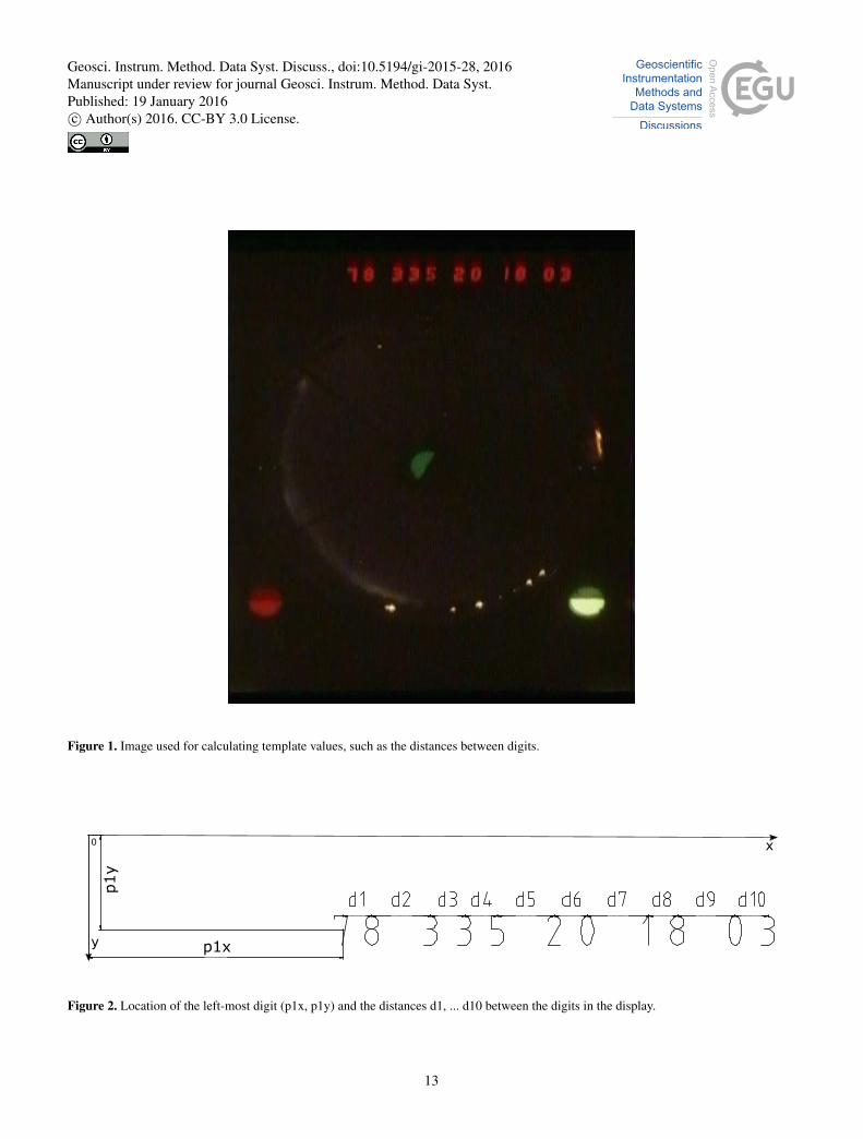
Figure 1. Image used for calculating template values, such as the distances between digits.

Figure 2. Location of the left-most digit (p1x, p1y) and the distances d1, ... d10 between the digits in the display.

13


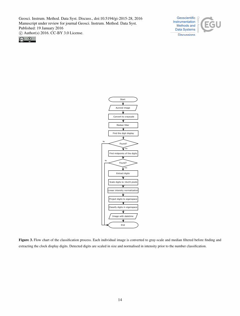
Figure 3. Flow chart of the classification process. Each individual image is converted to gray-scale and median filtered before finding and

extracting the clock display digits. Detected digits are scaled in size and normalised in intensity prior to the number classification.

14


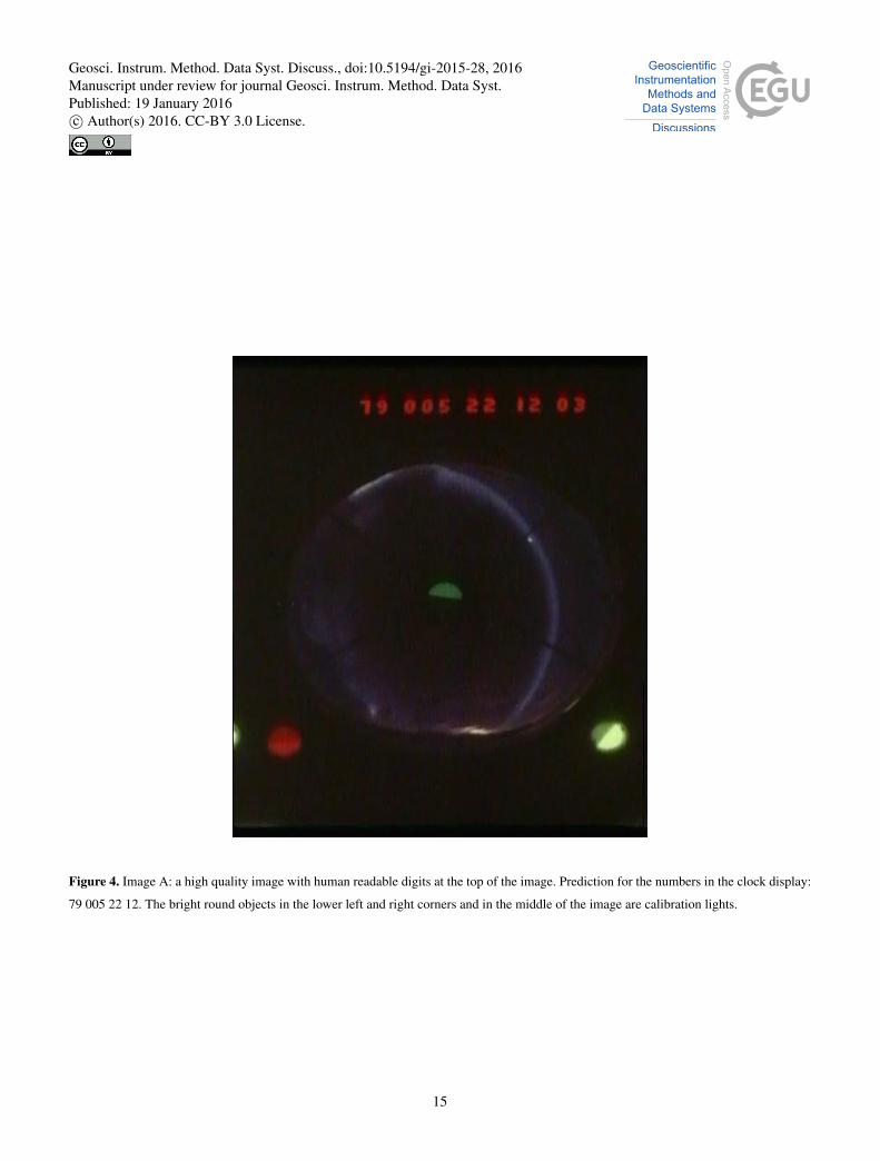
Figure 4. Image A: a high quality image with human readable digits at the top of the image. Prediction for the numbers in the clock display:

79 005 22 12. The bright round objects in the lower left and right corners and in the middle of the image are calibration lights.

15


Figure 5. Image B: a fair quality image with approximately human readable digits. Prediction: 90 314 03 36. The bright round object on the

right hand side of the image is the moon.

16


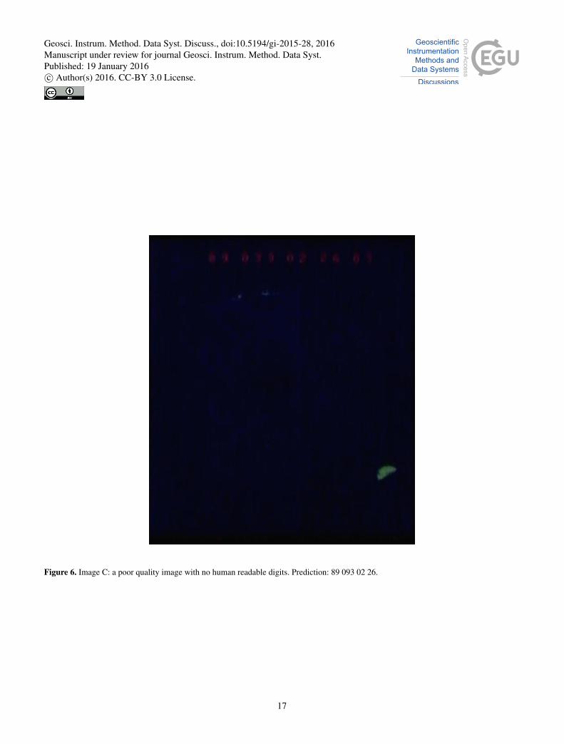
Figure 6. Image C: a poor quality image with no human readable digits. Prediction: 89 093 02 26.

17


0 100200300400500x-coordinate

5

10

15

intensity

Image A

0 100200300400500x-coordinate

5

10

15

20

intensity

Image B

0 100200300400500x-coordinate

3.0

3.5

4.0

4.5

intensity

Image C

Column-summed intensities, Original Image

Figure 7. The column-summed intensities of the clock display intensities of images A, B and C (figures 4, 5 and 6).

18


0 100200300400500x-coordinate

5

10

15

intensity

Image A

0 100200300400500x-coordinate

5

10

15

20

intensity

Image B

0 100200300400500x-coordinate

3.0

3.5

4.0

4.5

intensity

Image C

Column-summed intensities, Median Filtered Image

Figure 8. The column-summed intensities of the clock displays of images A, B and C (figures 4, 5 and 6) after median filtering.

19


0 100 200 300 400x-coordinate

1

2

3

4

5

6

7

intensity

Image A

0 100 200 300 400x-coordinate

2

3

4

5

6

intensity

Image B

0 100 200 300 400x-coordinate

1.0

1.5

2.0

intensity

Image C

Column-summed intensities, Smaller Image

Figure 9. The column-summed intensities of the clock displays of images A, B and C after extracting the clock display from the full image.

20


0 100 200 300 400x-coordinate

0.2

0.4

0.6

0.8

1.0

1.2

1.4

intensity

Image A

0 100 200 300 400x-coordinate

0.2

0.4

0.6

0.8

1.0

intensity

Image B

0 100 200 300 400x-coordinate

0.05

0.10

0.15

intensity

Image C

Column-summed intensities, Squared Image

Figure 10. The column-summed intensities for images A, B, and C after squaring the pixel intensities

21


0 100 200 300 400x-coordinate

0.0

0.2

0.4

0.6

0.8

1.0

1.2

1.4

intensity

Image A

0 100 200 300 400x-coordinate

0.0

0.2

0.4

0.6

0.8

1.0

intensity

Image B

0 100 200 300 400x-coordinate

0.00

0.05

0.10

0.15

intensity

Image C

Column-summed intensities, Average Filtered

Figure 11. Average filtered column-summed intensities of the previous figure.

22


0 100 200 300 400x-coordinate

0.0

0.2

0.4

0.6

0.8

1.0

1.2

1.4

intensity

Image A

0 100 200 300 400x-coordinate

0.0

0.2

0.4

0.6

0.8

1.0

intensity

Image B

0 100 200 300 400x-coordinate

0.00

0.05

0.10

0.15

intensity

Image C

Column-summed intensities, Signal After Morphology

Figure 12. The column-summed intensities of images A, B and C after applying a closing operator.

23


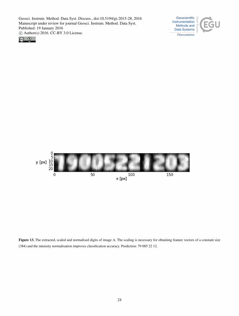
Figure 13. The extracted, scaled and normalised digits of image A. The scaling is necessary for obtaining feature vectors of a constant size

(384) and the intensity normalisation improves classification accuracy. Prediction: 79 005 22 12.

24


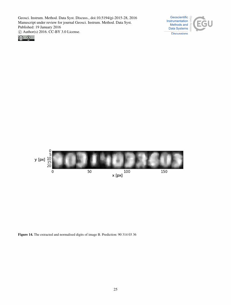
Figure 14. The extracted and normalised digits of image B. Prediction: 90 314 03 36

25


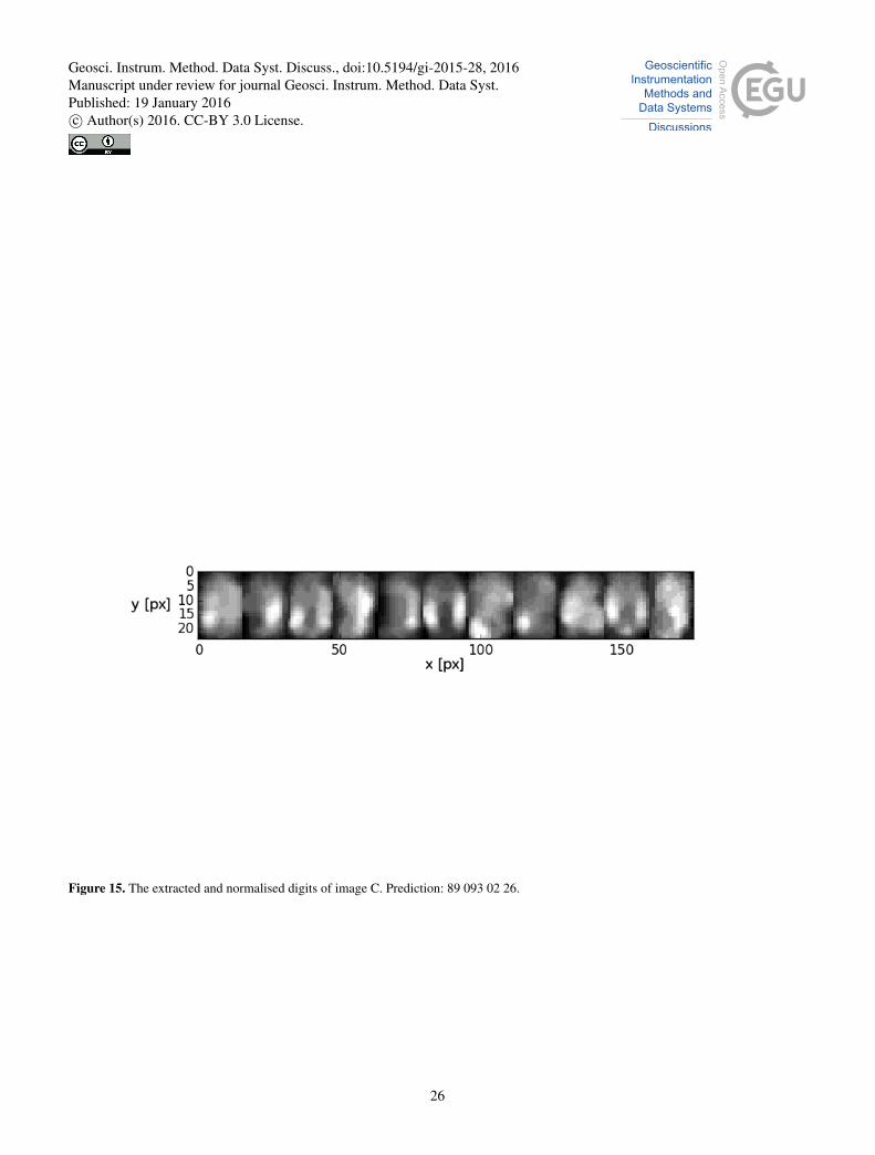
Figure 15. The extracted and normalised digits of image C. Prediction: 89 093 02 26.

26


Automatic segmentation and classication of seven-segment ......Automatic segmentation and...

Documents

Transcript of Automatic segmentation and classication of seven-segment ......Automatic segmentation and...